online extreme evolutionary learning machines · online extreme evolutionary learning machines ......

Online Extreme Evolutionary Learning Machines

Joshua E. Auerbach1, Chrisantha Fernando2 and Dario Floreano1

1Laboratory of Intelligent Systems, Ecole Polytechnique Federale de Lausanne (EPFL), Lausanne, Switzerland2School of Electronic Engineering and Computer Science, Queen Mary, University of London, London, UK

[email protected]

Abstract

Recently, the notion that the brain is fundamentally a pre-diction machine has gained traction within the cognitive sci-ence community. Consequently, the ability to learn accu-rate predictors from experience is crucial to creating intel-ligent robots. However, in order to make accurate predic-tions it is necessary to find appropriate data representationsfrom which to learn. Finding such data representations orfeatures is a fundamental challenge for machine learning. Of-ten domain knowledge is employed to design useful featuresfor specific problems, but learning representations in a do-main independent manner is highly desirable. While manyapproaches for automatic feature extraction exist, they are of-ten either computationally expensive or of marginal utility.On the other hand, methods such as Extreme Learning Ma-chines (ELMs) have recently gained popularity as efficientand accurate model learners by employing large collectionsof fixed, random features. The computational efficiency ofthese approaches becomes particularly relevant when learn-ing is done fully online, such as is the case for robots learn-ing via their interactions with the world. Selectionist meth-ods, which replace features offering low utility with randomreplacements, have been shown to produce efficient featurelearning in one class of ELM. In this paper we demonstratethat a Darwinian neurodynamic approach of feature replica-tion can improve performance beyond selection alone, andmay offer a path towards effective learning of predictive mod-els in robotic agents.

IntroductionThe notion of the brain as fundamentally a prediction ma-chine is an old idea (Helmholtz, 1860) that has recentlybeen gaining traction within the cognitive science commu-nity (see e.g. Clark, 2013; Hawkins and Blakeslee, 2007). Aconsequence of this idea is that if we wish to build robots ca-pable of exhibiting intelligent behavior, and adapting to dif-ferent circumstances, then prediction must be a fundamentalpart of their cognitive architecture. If the world behavedin a fundamentally linear way, than this would be an easyproblem to solve: linear models operating directly on rawsensorimotor data could be learned in a straightforward andefficient manner. Unfortunately, the world is noisy and fullof non-linear interactions that make learning difficult (Enns,

2010). In order to make accurate, non-linear predictions itis necessary to find appropriate data representations fromwhich to learn. Finding such data representations or featuresis a fundamental challenge for machine learning.

Often the domain knowledge of human experts is lever-aged to design useful features for specific problems (LeCunet al., 1998). While this may be an effective means of mak-ing learning tractable in many instances, it is not an idealsolution. Using human expertise is problem-specific, expen-sive, injects potentially sub-optimal biases into the solution,and for many robotics applications (especially those em-ploying soft materials or other unconventional components,e.g. Germann et al., 2014) the relevant expertise may not ex-ist. For these reasons, learning representations in a domainindependent manner is highly desirable.

One common method of predicting non-linear relation-ships is to train multilayer feed-forward neural networks,which have been proven to be universal function approxima-tors (Cybenko, 1989; Hornik, 1991). Most frequently thesenetworks are trained offline from a pre-compiled training-setof input and target output values by gradient-descent via thebackpropagation algorithm (Rumelhart et al., 1988). Thisoffers one approach to feature learning: by backpropagat-ing the supervised error signal, features can be adjusted inthe gradient-descent direction. While this method may worksuccessfully in many applications, it often learns slowly andmay require large datasets to be effective (Ciresan et al.,2010).

Many other approaches for automatic feature extractionhave been proposed in the literature. One approach that hasrecently proven quite successful involves the use an unsu-pervised “pre-training” step followed by further refinementthrough error backpropagation (Hinton and Salakhutdinov,2006). However, this method is computationally expensive–usually involving extended computation time even whenspecialized hardware is employed. Moreover, the necessityof doing extensive “pre-training” on a data set cannot be ap-plied when learning must be done fully online.

In online learning, data is learned from as it is received.In this regime, previously seen data points cannot be revis-

ALIFE 14: Proceedings of the Fourteenth International Conference on the Synthesis and Simulation of Living Systems

blriley

Typewritten Text

DOI: http://dx.doi.org/10.7551/978-0-262-32621-6-ch076

ited, and training gradients must be estimated from one (ora small subset) of the most recently seen data points. How-ever, learning online from data as it is obtained is crucial inrobotics domains where it is not possible to collect data apriori to be used in an offline batch mode. Moreover, evenif possible, batch learning is not always desirable, becauserobotic agents may be operating in non-stationary environ-ments within which they must continuously adapt. Finally,the volume of sensorimotor data obtained by agents mayeasily exceed the storage capacities of their onboard com-puters, especially if the agents continuously operate for ex-tended time periods. For these reasons, this work concernsitself with online learning of predictors.

An alternative approach to the above methods, which hasproven surprisingly effective, both for offline as well as on-line learning, is to randomly generate a large number offeatures on which to learn. Extreme Learning Machines(ELMs) (Huang et al., 2012) are a recently introduced for-malization of single-hidden-layer feed-forward neural net-works, where the feature-mappings are not tuned, but ratherare chosen stochastically. This has the advantage that theonly model parameters that are trained are the connectionweights from hidden units to outputs, therefore simplifyinglearning to a linear regression problem1. The intuition hereis that these fixed random features create a dimensionalityexpansion on top of which it is often possible to fit a linearmodel.

Recent work has demonstrated that it is possible to au-tomatically search for effective features in online learningscenarios through a generate and test procedure (Mahmoodand Sutton, 2013). In that work, it was demonstrated that, ina form of ELM-like artificial neural network (ANN), predic-tive accuracy could be greatly improved by regularly dis-carding features that offer low utility and replacing themwith new stochastically generated features. This is essen-tially a selectionist approach, whereby poor features are se-lected for elimination and new features are generated in acompletely random manner devoid of any information trans-fer.

In this work we extend Mahmood and Sutton’s approachby taking inspiration from the Neuronal Replicator Hypoth-esis (Fernando et al., 2010, 2012), which posits that “repli-cation (with mutation) of patterns of neuronal activity canoccur within the brain using known neurophysiological pro-cesses.” Specifically, instead of introducing new featuresat random as Mahmood and Sutton have done, new fea-tures are created through a Darwinian process of replica-tion + variation of existing features, which have been dis-

1Echo State Networks (Becker and Obermayer, 2003) and Liq-uid State Machines (Maass et al., 2002) (collectively known asReservoir Computing) employ a similar idea for recurrent neuralnetworks: the output connections from a dynamical reservoir ofstochastically generated neurons is trained to fit a teaching signalvia linear regression

covered to be useful for solving the given prediction prob-lem2. We dub this learning architecture an Online ExtremeEvolutionary Learning Machine (OEELM). We demonstratethat OEELMs are capable of achieving lower error thanthe purely selectionist approach employed in (Mahmoodand Sutton, 2013) with a much smaller number of features.Moreover we demonstrate that this method compares favor-ably to backpropagation.

The remainder of this paper is structured as follows. Thefollowing section describes the OEELM method, and de-scribes the experimental setup used for comparing this ap-proach to existing methods. Next, the results of these ex-periments are presented and analyzed. A discussion of thismethod is then presented, followed by conclusions and di-rections for future research.

MethodsTaking inspiration from Mahmood and Sutton (2013), we in-vestigate the problem of automatically searching for usefulfeatures in a fully online learning scenario. In this formula-tion, an ANN is attempting to learn by adjusting its parame-ters to better fit the observations emanating from a noisy datastream. The underlying learning architecture is an ELM-like, single-hidden-layer feed-forward ANN. Following theimplementation described in (Mahmood and Sutton, 2013)the ANN architecture consists of an input layer fully con-nected to a hidden layer with nonlinear activation functions(all features have access to all inputs), which is then fullyconnected to a linear output unit that produces a predictionof a target value.

The nonlinearities in the hidden layer are achieved bymeans of Linear Threshold Units (LTUs) adopted from (Sut-ton and Whitehead, 1993). Specifically, the output of featurei is given as follows:

fi(x(t)) =

{1 if

∑mj=1 v

(t)ji x

(t)j > θ

(t)i

0 otherwise∀i = 1, ..., n (1)

for a network with m inputs and n features. Here, x(t) is theinput vector at iteration t, v(t)ji is the weight from input j to

feature i at iteration t, x(t)j is the jth component of x(t), and

θ(t)i is the threshold of feature i at iteration t.

The prediction of the network at iteration t is given by

y(t) =

n∑i=0

w(t)i fi(x

(t)) (2)

where f0(x) is a bias feature that is always set to 1.At each iteration t, the network is presented with a sin-

gle observation (x(t), y(t)) from a noisy data stream and the

2It is worth stressing that, here, we evolve a population of fea-tures for a single predictor, rather than a population of predictorsas in (Arthur, 1994; Bongard and Lipson, 2007).


output weights w are updated in order to reduce the meansquared error between the observed target value y(t) and thepredicted value y(t) by means of the Delta-rule (Widrow andHoff, 1960):

∆w(t)i = η(y(t) − y(t))fi(x(t)) (3)

w(t+1)i = w

(t)i + ∆w

(t)i (4)

where η is a free parameter known as the learning rate.

Feature SelectionMahmood and Sutton (2013) demonstrated that the predic-tive accuracy of this class of model could be improved if,instead of using a fixed random set of feature weights v, se-lection is employed to discard features offering low utilityand replace them with new features during the course of on-line learning. One problem with implementing such a selec-tionist method in an online setting is that it may be difficultto quantify the utility of individual features. As argued inthat work, if a batch learning system is optimized until con-vergence (see e.g. Schmidhuber et al., 2007) then the utilityof features can easily be evaluated, but in an online settingthis evaluation must be able to function on a per-example ba-sis. Additionally, it is argued in Mahmood and Sutton (2013)that in online settings, where new data points are constantlyarriving, the process of evaluating feature utilities must becomputationally efficient and not add to the overall compu-tational complexity of the learning system.

Mahmood and Sutton (2013) present a method that over-comes these limitations. For each iteration of online learn-ing, a small fraction ρ of existing features is selected forelimination and replaced with newly generated, random fea-tures. They demonstrate that such an approach can be im-plemented such that the total computational complexity isno greater than a base system that implements the Delta-rule for learning the readout weights: O(mn) for computingthe output of the ANN, and O(n) for updating the readoutweights. The reader is referred to that work for further de-tails of this derivation.

Finally, that work presented three alternative approachesfor estimating the utility of a feature in the online learningscenario. All three of the approaches are based upon the ideathat the relative utility of a feature is related to the magnitudeof its readout weight. The intuition behind this idea is thatthe magnitude of a feature’s readout weight determines howmuch that feature contributes to the output of the network.Since the readout weights are trained to approximate the ob-served data, the magnitude of a feature’s readout weight willtherefore serve as a proxy for how much that feature servesto explain the observations.

The problem with using the actual readout weight magni-tude of a feature is that newly introduced features will ini-tially have small output weight magnitudes3, and without a

3Newly introduced features are initially given a readout weight

mechanism to allow them time to prove their usefulness theywill immediately be selected for elimination. Here, we adoptone of the procedures described in that work for overcomingthis difficulty. This is described next.

In the employed approach, the utility of a feature ui iscalculated as an exponential moving average (EMA) of themagnitude of its readout weight:

u(t+1)i = αuu

(t)i + (1− αu)|w(t+1)

i | (5)

where αu is the decay rate of the EMA, here chosen througha tuning procedure to be 0.9.

When a new feature k is introduced, uk is set to the me-dian utility value of all features so that it does not get re-placed immediately. If this new feature is not useful then itsactual readout weight wk will remain near zero, and there-fore uk will shrink over time. This will lead to feature keventually getting replaced. On the other hand, if featurek is useful then wk will increase in magnitude and the fea-ture will remain in the network. We choose this particularprocedure because it performed competitively with the otherapproaches described in (Mahmood and Sutton, 2013), andis straightforward to implement.

Feature EvolutionThe technique of (Mahmood and Sutton, 2013) describedabove is purely selectionist: features with poor utility are se-lected for elimination and are replaced with features that aregenerated at random. However, it is known that purely se-lectionist search methods have limitations that may be over-come through the use of replicators (Fernando et al., 2010).Additionally, there is a growing body of evidence which sug-gests that there is a process of replication occuring within in-dividual brains (Fernando et al., 2010, 2012). Taking theseideas as inspiration, we suggest that a Darwinian process offeature evolution (with replication) will be a more powerfulsearch method than the purely selectionist approach.

Extending the above selectionist method into a Darwinianone is fairly straightforward. The process of estimating fea-ture utility and selecting features for removal remains un-changed. The main difference is that this utility estimationbecomes the fitness function on which an online (steady-state) evolutionary algorithm operates. Now, instead of in-troducing new features purely at random, eliminated fea-tures are replaced with mutated copies of other features,which have themselves proved to be useful for explainingthe observed data.

Specifically, when a feature is selected for removal, a bi-nary tournament is conducted to choose a “parent” featurefor reproduction. Two features from the population are cho-sen at random and the one with higher fitness creates a copyof itself. Each gene of that feature (the weights vji) are then

of 0 so that they do not to contribute to the prediction before thelearner has a chance to adjust this weight.


Figure 1: Comparison of learning errors across regimes and number of features. Left: this plot depicts how predictive-error(calculated as the mean across 30 independent runs of a sliding window estimate of mean squared error) varies over training timefor all experimental setups investigated. Right: boxplots comparing the predictive-errors across regimes after being exposed to1,000,000 examples. Asterisks denote statistical significance (*** = p-value < 0.001, Mann-Whitney U test with Bonferronicorrection).

mutated with probability pmutate and the resulting feature re-places the removed one. As is the case in the selectionistmethod, the readout weight of this feature is initialized to 0,and its fitness is initialized to the median fitness of the popu-lation. Conducting a binary tournament takes constant time(since the fitnesses are already in memory) and mutating thewinner takes no more time than creating a new feature atrandom: O(m). Therefore, the evolutionary approach is nomore computationally expensive than the selectionist one.

ExperimentsWe first reproduce the results presented in (Mahmood andSutton, 2013) before comparing the selectionist approachwith the evolutionary approach. These experiments are de-scribed here.

Refer back to Eqn. 1. In these experiments the systemis assumed to take a binary input vector x ∈ {0, 1}m andproduce a scalar prediction y ∈ R. The input weights vjiare initialized with either +1 or −1 uniformly at random.The threshold θi is set as θi = mβi − Si, where Si is thenumber of negative input weights of feature i and βi is a freeparameter. This formulation ensures feature i activates whenat least mβi input bits match the prototype defined by thefeature’s weights. Following the procedure of (Mahmoodand Sutton, 2013)4 βi is set to 0.6 ∀i.

In the absence of any feature search procedure the valuesof these parameters will remain fixed for the entire durationof an online learning task–the network is essentially an ELMwith binary features. However, when either the selectionistor the evolutionary approach is employed, its task is to find aset of features that is appropriate for explaining the observeddata.

4Clarified in (Mahmood, 2014).

The online learning task is conducted in simulation. Ateach iteration a binary, 20-dimensional input vector x(t) isgenerated uniformly at random. This input is fed through anANN of the type described above containing 20 fixed ran-dom LTU target features f∗i each having threshold parame-ter βi = 0.6. Next, the outputs of these features are linearlycombined with output weights drawn from a normal distri-bution having mean 0 and unit variance (w∗

i ∼ N(0, 1)).The output of this network is then injected with Guassiannoise εt ∼ N(0, 1) drawn independently at random for eachiteration. Summarizing, the target value at iteration t, yt iscomputed as:

yt =

20∑i=1

w∗i f

∗i + εt (6)

The Gaussian noise makes the task more resemble real-world online learning tasks such as those found in roboticsapplications, and implies that if the learning network exactlylearns the target function than the expected value of its meansquared error will be 1.

At each iteration, the learning rate η is set to γλ(t) , where

γ ∈ (0, 1) is the effective learning rate5, and λ(t) is an EMAestimate of the squared norm of the feature vector:

λ(t) = αλλ(t−1) + (1− αλ)(f (t−1) · f (t−1)) (7)

Unless otherwise specified, all reported results employ a de-cay rate αλ = 0.999, and an effective learning rate γ = 0.1.

ResultsThe above online learning problem is investigated underseveral experimental regimes. The first regime: “no selec-

5Called the effective step-size in Mahmood and Sutton’s termi-nology.


Figure 2: Exploring non-stationary environments. Here the environment (the target function) switches between two randomlygenerated functions every 100,000 iterations. Left: the same learning algorithms as are used for stationary environments. Right:for both the “selection” and “evolution” regimes features may be added to a growing archive that is immune from selection.These plots depict how predictive-error (calculated as the mean across 30 independent runs of a sliding window estimate ofmean squared error) varies over training time.

tion” employs a fixed, random feature set, as is tradition-ally used in ELMs. The second regime: “selection” usesthe purely selectionist approach of Mahmood and Sutton(2013). The third regime: “evolution” uses the evolutionaryapproach based on Darwinian neurodynamics introducedabove (OEELMs). Each regime is investigated for differ-ent, fixed, number of features n. For each regime and valueof n, 30 independent runs of the online learning scenario areconducted. Each learning scenario lasts for 1,000,000 itera-tions.

Under both the “selection” and “evolution” regimes, thefraction ρ = 0.005 of the existing features having lowest es-timated utility are selected for elimination at each iteration.Under the “evolution” regime, the input weights of copiedfeatures are each mutated with probability pmutate = 0.1,chosen to optimize performance. Reported results are robustto small variations of this value.

Fig. 1 compares the performance of these regimes as thelearning experiments progress. On the left, the accuracyof each experimental setup (regime and n value) is plottedfor each iteration t as follows. Within each run, the cur-rent mean squared error (MSE) is estimated using a slidingwindow approach: the current error estimate is the mean ofthe individual squared errors of the past 10,000 data points.Due to the noise inherent in the data stream, the sliding win-dow provides a better estimate of a predictor’s accuracy at agiven time than its error on any individual data point. Themeans of these MSE estimates are then taken across the 30independent runs of each experimental setup. On the right,we show a boxplot comparing the most relevant final MSEestimates after 1,000,000 iterations.

With a fixed, random feature set (the “no selection”regime) performance improves as a function of the num-ber of features, but continuing to increase the feature count

has diminishing returns. As demonstrated by Mahmoodand Sutton (2013), and confirmed here, a purely selectionistapproach to searching for features (the “selection” regime)with only 1,000 features can outperform a fixed feature setof 1,000,000 features. However, by using the OEELM ap-proach described above, near optimal error can be achievedvery rapidly. Moreover, using only 100 features with “evo-lution” not only outperforms all “no selection” formulationsinvestigated, but also all “selection” formulations as well.Using 100 features with “evolution”, the estimated MSEbecomes significantly smaller (p-value < 0.001, Mann-Whitney U test) than that of all “no selection” and “selec-tion” setups by iteration 104,900 and remains that way forthe duration of the learning scenarios.

Non-stationary EnvironmentsOften robotic agents are operating in non-stationary envi-ronments to which they must continuously adapt. In orderto investigate whether feature evolution is also useful underchanging environmental conditions the above online learn-ing task is altered as follows. Instead of having a single tar-get function that a network is attempting to predict, two dif-ferent target functions are created. Since it is likely that dif-ferent environmental conditions will have many similarities(e.g. the laws of physics remain unchanged across environ-ments), the two functions are related to each other. Specifi-cally, target function 1 is constructed exactly the same wayas described above. Target function 2 is constructed fromtarget function 1 by replacing 25% of its hidden nodes. Foreach node to be replaced, a new input weight vector is cre-ated uniformly at random, and a new readout weight is cho-sen from a Gaussian distribution with zero mean and unitvariance.

The experimental procedure above is repeated for this


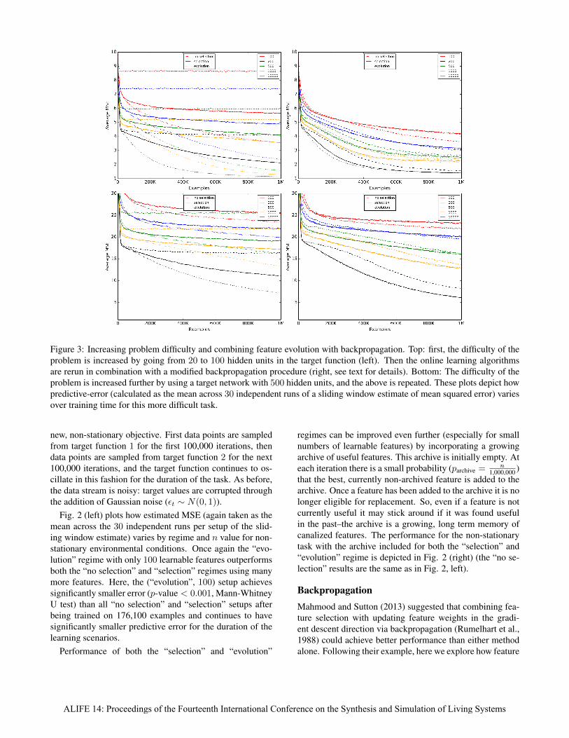
Figure 3: Increasing problem difficulty and combining feature evolution with backpropagation. Top: first, the difficulty of theproblem is increased by going from 20 to 100 hidden units in the target function (left). Then the online learning algorithmsare rerun in combination with a modified backpropagation procedure (right, see text for details). Bottom: The difficulty of theproblem is increased further by using a target network with 500 hidden units, and the above is repeated. These plots depict howpredictive-error (calculated as the mean across 30 independent runs of a sliding window estimate of mean squared error) variesover training time for this more difficult task.

new, non-stationary objective. First data points are sampledfrom target function 1 for the first 100,000 iterations, thendata points are sampled from target function 2 for the next100,000 iterations, and the target function continues to os-cillate in this fashion for the duration of the task. As before,the data stream is noisy: target values are corrupted throughthe addition of Gaussian noise (εt ∼ N(0, 1)).

Fig. 2 (left) plots how estimated MSE (again taken as themean across the 30 independent runs per setup of the slid-ing window estimate) varies by regime and n value for non-stationary environmental conditions. Once again the “evo-lution” regime with only 100 learnable features outperformsboth the “no selection” and “selection” regimes using manymore features. Here, the (“evolution”, 100) setup achievessignificantly smaller error (p-value < 0.001, Mann-WhitneyU test) than all “no selection” and “selection” setups afterbeing trained on 176,100 examples and continues to havesignificantly smaller predictive error for the duration of thelearning scenarios.

Performance of both the “selection” and “evolution”

regimes can be improved even further (especially for smallnumbers of learnable features) by incorporating a growingarchive of useful features. This archive is initially empty. Ateach iteration there is a small probability (parchive = n

1,000,000 )that the best, currently non-archived feature is added to thearchive. Once a feature has been added to the archive it is nolonger eligible for replacement. So, even if a feature is notcurrently useful it may stick around if it was found usefulin the past–the archive is a growing, long term memory ofcanalized features. The performance for the non-stationarytask with the archive included for both the “selection” and“evolution” regime is depicted in Fig. 2 (right) (the “no se-lection” results are the same as in Fig. 2, left).

BackpropagationMahmood and Sutton (2013) suggested that combining fea-ture selection with updating feature weights in the gradi-ent descent direction via backpropagation (Rumelhart et al.,1988) could achieve better performance than either methodalone. Following their example, here we explore how feature


evolution might synergize with backpropagation. Specifi-cally, we employ the modified version of backpropagationintroduced in that work: the output weights are adjusted us-ing the Delta-rule as above, but since LTUs do not vary con-tinuously, the gradient of each hidden unit is estimated usinga logistic function centered around the threshold of its LTU.Then, instead of using the magnitude of the error multipliedby the output weights (y(t) − y(t))w(t)

i when computing thefeature gradients, only the sign of this quantity is taken, sothat feature weights vji are updated as follows:

v(t+1)ji = v

(t)ji + ηinput ∗ sign((y(t) − y(t))w(t)

i )

∗σi(x(t))(1− σi(x(t)))x(t)j

where σi(x(t)) = 1

1+e−(v

(t)jix(t)j

−β(t)i

)is the logistic function

activation of the ith feature, and the learning rate ηinput wasselected by tuning to be a constant value of 0.01.

In order to investigate how feature evolution synergizeswith backpropagation, we conduct further experiments.First, we make the learning problem more difficult by in-creasing the number of hidden units in the target network,then we supplement the above learning methods by firstbackpropagating the error before performing feature selec-tion or evolution.

Fig. 3 shows how the performance of the experimentalsetups vary when the number of hidden units in the targetnetwork is increased to either 100 or 500. The left sideof these figures uses the experimental setups as describedabove where only the readout weights are adjusted via theDelta-rule, the right side of these figures additionally incor-porate the modified backpropagation just described. Theseresults are discussed below.

DiscussionLooking at the left hand plots of Fig. 3 we see that as theproblem is made more difficult, the advantage conferred byfeature evolution appears to decrease. While the best per-formances are still found in the “evolution” regime, it nowrequires 500 learnable features to outperform selection with10,000 learnable features in the 100 hidden target case, andrequires 10,000 learnable features to do so when there are500 hidden units in the target network. This could be forseveral reasons: one possibility is that as the prediction prob-lem becomes more complex the necessity of maintaining adiverse set of features becomes more pressing. The “selec-tion” regime naturally accomplishes this by introducing newfeatures that are unrelated to existing features. Finding ef-fective, computationally inexpensive methods for promotingfeature diversity in the “evolution” regime will require fur-ther work.

For these experiments, altering the learning procedure toinclude backpropagation of error drastically improves theperformance of the “no selection” regime (Fig. 3, right hand

plots). This is essentially going from linear regression tothe typical supervised ANN learning procedure. The perfor-mance of the “selection” regime is also either improved orleft approximately the same. However, feature evolution nolonger affects much improvement beyond purely selectionistmethods.

This last point may be due to how feature weights arereplicated. Here, the genome of a feature is considered tobe its initial input weight vector, not the weight vector thathas been altered through backpropagation–the evolutionaryprocess is Darwinian rather than Lamarckian. So, any use-ful feature learning that arises as a result of backpropagationis not inherited through reproduction, and newly born fea-tures must then learn the backpropagated weight changesanew–just as under the selectionist method. Lamarckianevolution is known to be unstable in dynamic environmentsover phylogenetic timescales (Sasaki and Tokoro, 1997), butwhether Lamarckian evolutionary neurodynamics combinedwith backpropagation also falls victim to the same patholo-gies remains to be tested in future work.

ConclusionIn this work we have introduced a method (Online ExtremeEvolutionary Learning Machines) for automatically search-ing for features in an online learning task through featurereplication. This process essentially makes the features(ANN hidden nodes) the members of a population under-going an online, steady state evolutionary algorithm. Wehave demonstrated that using OEELMs results in signifi-cantly better predictive accuracy as compared to either usinga fixed set of features or a purely selectionist search method,for both stationary and non-stationary environments.

Additionally, we have explored feature evolution as it re-lates to learning features through the backpropagation of er-ror. Here, feature evolution is capable of achieving similaror better error than backpropagation in many instances (seeFig. 3). This result alone is interesting, because feature evo-lution may be more widely applicable than backpropagation:it does not require having known, differentiable features, butin principle could be used to evolve features of any form.Another natural next step is the application of evolution toconvolutional neural networks (LeCun and Bengio, 1995).Here instead of hand-designing the shapes of the kernels thatproduce feature maps, the shapes and properties of kernelsthemselves can be evolved. Finally, it will be worthwhileto investigate how encoding features with a more evolvable,indirect encoding such as HyperNEAT (Stanley et al., 2009)may improve performance even further.

Feature evolution, as inspired by the Neuronal Replica-tor Hypothesis, is a promising method for online learningtasks. We foresee it being of particular relevance for roboticsapplications, where robots must learn predictive models inorder to operate in unknown and possibly non-stationaryenvironments. Specifically, we foresee these methods be-


ing useful for a robot to learn forward and inverse mod-els (Wolpert and Kawato, 1998) from which it may fanta-size against in order to accomplish some task in a given en-vironment. This should allow for a robot to easily adaptto damage (Bongard et al., 2006) or to changes in mor-phology brought about by evolution, development or self-reconfiguration. This promising area will be investigated infuture work.

Source CodeThe source code used for all experiments conducted inthis paper is available online at https://github.com/jauerb/OEELM.

AcknowledgementsThe authors thank Rupam Mahmood for his kind coopera-tion and advice.The research leading to these results has received fundingfrom the European Union Seventh Framework Programme(FP7/2007-2013) under grant agreement n◦ 308943 and the“Bayes, Darwin, and Hebb” Templeton Foundation FQEBGrant.

ReferencesArthur, W. B. (1994). Inductive reasoning and bounded rationality.

American Economic Review, 84(2):406–411.

Becker, S. T. S. and Obermayer, K., editors (2003). Adaptive non-linear system identification with echo state networks. MITPress Cambridge, MA.

Bongard, J. and Lipson, H. (2007). Automated reverse engineeringof nonlinear dynamical systems. Proceedings of the NationalAcademy of Science, 104(24):9943–9948.

Bongard, J., Zykov, V., and Lipson, H. (2006). Resilient machinesthrough continuous self-modeling. Science, 314:1118–1121.

Ciresan, D. C., Meier, U., Gambardella, L. M., and Schmidhuber,J. (2010). Deep, big, simple neural nets for handwritten digitrecognition. Neural computation, 22(12):3207–3220.

Clark, A. (2013). Whatever next? predictive brains, situatedagents, and the future of cognitive science. Behavioral andBrain Sciences, 36(03):181–204.

Cybenko, G. (1989). Approximation by superpositions of a sig-moidal function. Mathematics of control, signals and sys-tems, 2(4):303–314.

Enns, R. H. (2010). It’s a Nonlinear World. Springer.

Fernando, C., Goldstein, R., and Szathmary, E. (2010). Theneuronal replicator hypothesis. Neural computation,22(11):2809–2857.

Fernando, C. T., Szathmary, E., and Husbands, P. (2012). Se-lectionist and evolutionary approaches to brain function: acritical appraisal. Frontiers in Computational Neuroscience,6(24).

Germann, J., Auerbach, J., and Floreano, D. (2014). Programmableself-assembly with chained soft modules: an algorithm tofold into any 2-d shape. In Proceedings of the InternationalConference on the Simulation of Adaptive Behavior. To Ap-pear.

Hawkins, J. and Blakeslee, S. (2007). On Intelligence. Macmillan.

Helmholtz, H. v. (1860). Handbuch der physiologischen optik, vol.& trans. jpc southall.

Hinton, G. E. and Salakhutdinov, R. R. (2006). Reducingthe dimensionality of data with neural networks. Science,313(5786):504–507.

Hornik, K. (1991). Approximation capabilities of multilayer feed-forward networks. Neural networks, 4(2):251–257.

Huang, G.-B., Zhou, H., Ding, X., and Zhang, R. (2012). Extremelearning machine for regression and multiclass classification.Systems, Man, and Cybernetics, Part B: Cybernetics, IEEETransactions on, 42(2):513–529.

LeCun, Y. and Bengio, Y. (1995). Convolutional networks for im-ages, speech, and time series. The handbook of brain theoryand neural networks, 3361.

LeCun, Y., Bottou, L., Bengio, Y., and Haffner, P. (1998). Gradient-based learning applied to document recognition. Proceedingsof the IEEE, 86(11):2278–2324.

Maass, W., Natschlager, T., and Markram, H. (2002). Real-timecomputing without stable states: A new framework for neu-ral computation based on perturbations. Neural computation,14(11):2531–2560.

Mahmood, A. R. (2014). Personal Communication.

Mahmood, A. R. and Sutton, R. S. (2013). Representation searchthrough generate and test. In Workshops at the Twenty-Seventh AAAI Conference on Artificial Intelligence.

Rumelhart, D. E., Hinton, G. E., and Williams, R. J. (1988). Learn-ing representations by back-propagating errors. MIT Press,Cambridge, MA, USA.

Sasaki, T. and Tokoro, M. (1997). Adaptation toward changingenvironments: Why darwinian in nature. In Fourth Europeanconference on artificial life, pages 145–153. MIT Press.

Schmidhuber, J., Wierstra, D., Gagliolo, M., and Gomez, F. (2007).Training recurrent networks by evolino. Neural computation,19(3):757–779.

Stanley, K., D’Ambrosio, D., and Gauci, J. (2009). A hypercube-based encoding for evolving large-scale neural networks. Ar-tificial Life, 15(2):185–212.

Sutton, R. S. and Whitehead, S. D. e. a. (1993). Online learningwith random representations. In ICML, pages 314–321. Cite-seer.

Widrow, B. and Hoff, M. E. e. a. (1960). Adaptive switching cir-cuits. In IRE WESCON Conv. Rec., volume 4, pages 96–104.Defense Technical Information Center.

Wolpert, D. M. and Kawato, M. (1998). Multiple paired for-ward and inverse models for motor control. Neural Networks,11(7):1317–1329.


https://github.com/jauerb/OEELM

https://github.com/jauerb/OEELM

online extreme evolutionary learning machines · online extreme evolutionary learning machines ......

Documents