online discrete event control of hybrid systems c james …millan/thesis/jpmthesis.pdf · online...
TRANSCRIPT
Online Discrete Event Control of Hybrid Systems
by
c James P. Millan
B.Eng., Memorial University of Newfoundland, 1984
A thesis submitted to theSchool of Graduate Studiesin partial ful�llment of therequirements for the degree of
Doctor of Philosophy
Faculty of Engineering and Applied ScienceMemorial University of Newfoundland
October 2006
St.John�s Newfoundland

To my parents,
Steven and Brenda,
and for Les.
Online Discrete Event Control of Hybrid Systems
by
James P. Millan
Abstract
The increasing proliferation of automatic control systems in embedded and distributed
applications has lead to increasingly complex systems. These systems manifest a
mixture of continuous and discrete dynamics due to the interaction of the computer
controlled or logical decision-making subsystems interacting with the real world, and
are thus referred to as hybrid systems. The inherent complexity of such hybrid systems
makes them di¢ cult to model, analyze and design. As such, industrial application of
hybrid system theory has yet to gain widespread acceptance.
This thesis presents an approach to the modeling, synthesis and implementation of
automatic controllers for hybrid systems. This work centers on a �exible hybrid sys-
tem modeling framework that permits automated synthesis of controllers for hybrid
systems, based on safety and performance design speci�cations. This hybrid model-
ing framework is the switched continuous model (SCM), based on discrete switching
between continuous system models (CSM). Discrete abstractions of the CSM dynam-
ics enable the controller actions to be simple discrete decisions at appropriate points
in the state space of the controlled system. The SCM communicates with external
discrete event systems (DES) through sets of shared discrete events, thus allowing
ii
the techniques of DES supervisory control synthesis to be employed. The resulting
controllers are model-based, and safe by design, since they encapsulate the continuous
and discrete event models that together model the plant and speci�cation dynamics.
Due to the inherently uncountable state space of the hybrid system model, the con-
troller computation is performed online, and is limited to a �nite time horizon in
order to preserve the �nite state properties of the discrete abstraction.
The details of the modeling framework, controller synthesis, and online imple-
mentation are developed, including a computational approach, architecture, and al-
gorithms. A software package that implements these control concepts was developed.
Two detailed modeling and control synthesis applications are presented: a simple
benchmark hybrid control example and a realistic industrial example.
iii
.
Acknowledgements
I would like to take this opportunity to thank my thesis supervisor, Dr. Siu
O�Young for his untiring enthusiasm, optimism and guidance. Siu was instrumental in
encouraging me to enter graduate studies and later to pursue my Ph.D.; a somewhat
non-trivial task, considering the length of time that had elapsed since I had left
university (over 15 years). Although it has been challenging, I have enjoyed the
learning and the discovery that comes with graduate work.
I would like to thank my employer, the National Research Council, Institute for
Ocean Technology, for giving me the opportunity to change my career direction from
an instrumentation and control systems engineer to that of a researcher. I thank Mr.
David Murdey and Dr. Bruce Colbourne in that respect. Thanks to my co-worker
Dr. Wayne Raman-Nair for many discussions and advice on a wide range of topics
that proved to be useful to my thesis work, including solutions to ODEs, numerical
modeling, teaching, and how to write a Ph.D. dissertation.
I would like to thank my thesis committee, in particular Dr. Theo Norvell, for
their careful reading, and helpful corrections and suggestions.
Finally, and most importantly, I would like to thank my family; my wife Roxanne,
daughter Kelsey, and son Jonathan, for their patience and understanding while I
spent many hours working, especially in the past few months, as I completed this
document.
iv
Contents
Abstract ii
Acknowledgements iv
Contents v
List of Tables xi
List of Figures xii
List of Abbreviations xvii
1 Introduction 1
1.1 Background . . . . . . . . . . . . . . . . . . . . . . . . . . . . . . . . 1
1.2 Problem Discussion . . . . . . . . . . . . . . . . . . . . . . . . . . . . 3
1.3 Contributions . . . . . . . . . . . . . . . . . . . . . . . . . . . . . . . 4
1.4 Organization . . . . . . . . . . . . . . . . . . . . . . . . . . . . . . . 5
2 Background and Related Work 7
2.1 Continuous System Modeling and Control . . . . . . . . . . . . . . . 7
2.2 Discrete Event Systems . . . . . . . . . . . . . . . . . . . . . . . . . . 9
2.3 Hybrid System Modeling . . . . . . . . . . . . . . . . . . . . . . . . . 10
v
2.3.1 Timed Automata . . . . . . . . . . . . . . . . . . . . . . . . . 11
2.3.2 Hybrid Automata . . . . . . . . . . . . . . . . . . . . . . . . . 11
2.3.3 Quantized I/O (Discrete Event Abstraction) . . . . . . . . . . 13
2.3.4 Switched Systems . . . . . . . . . . . . . . . . . . . . . . . . . 14
2.4 Hybrid System Simulation . . . . . . . . . . . . . . . . . . . . . . . . 15
2.5 Complexity . . . . . . . . . . . . . . . . . . . . . . . . . . . . . . . . 16
2.6 Assessment of Relevant Work . . . . . . . . . . . . . . . . . . . . . . 17
2.6.1 Model Formulation . . . . . . . . . . . . . . . . . . . . . . . . 17
2.6.2 Discrete Abstraction . . . . . . . . . . . . . . . . . . . . . . . 18
2.6.3 Controller Synthesis . . . . . . . . . . . . . . . . . . . . . . . 18
2.6.4 Computation . . . . . . . . . . . . . . . . . . . . . . . . . . . 19
2.7 Summary . . . . . . . . . . . . . . . . . . . . . . . . . . . . . . . . . 20
3 Abstraction of Continuous System Dynamics 21
3.1 Introduction . . . . . . . . . . . . . . . . . . . . . . . . . . . . . . . . 21
3.2 State Quantization . . . . . . . . . . . . . . . . . . . . . . . . . . . . 25
3.3 Discrete Event Generation . . . . . . . . . . . . . . . . . . . . . . . . 33
3.4 Examples . . . . . . . . . . . . . . . . . . . . . . . . . . . . . . . . . 38
3.5 Conclusions . . . . . . . . . . . . . . . . . . . . . . . . . . . . . . . . 45
4 Switched Continuous Model 50
4.1 Introduction . . . . . . . . . . . . . . . . . . . . . . . . . . . . . . . . 50
4.2 Switched Continuous Model . . . . . . . . . . . . . . . . . . . . . . . 52
4.3 Prediction - Case I Switching . . . . . . . . . . . . . . . . . . . . . . 56
4.4 Prediction - Case II Switching . . . . . . . . . . . . . . . . . . . . . . 62
4.5 Continuous Dynamics . . . . . . . . . . . . . . . . . . . . . . . . . . . 66
4.6 Continuous State Reachability . . . . . . . . . . . . . . . . . . . . . . 70
4.6.1 Case I Switching . . . . . . . . . . . . . . . . . . . . . . . . . 70
4.6.2 Case II Switching . . . . . . . . . . . . . . . . . . . . . . . . . 71
vi
4.7 Discrete Event Dynamics . . . . . . . . . . . . . . . . . . . . . . . . . 73
4.7.1 Case I Switching . . . . . . . . . . . . . . . . . . . . . . . . . 73
4.7.2 Case II Switching . . . . . . . . . . . . . . . . . . . . . . . . . 74
4.8 Hybrid Transition Graph . . . . . . . . . . . . . . . . . . . . . . . . . 74
4.9 SCM Example . . . . . . . . . . . . . . . . . . . . . . . . . . . . . . . 82
4.10 Conclusions . . . . . . . . . . . . . . . . . . . . . . . . . . . . . . . . 84
5 Control of Hybrid Systems 88
5.1 Discrete Event Controller Synthesis . . . . . . . . . . . . . . . . . . . 89
5.2 SCM and Control Synthesis . . . . . . . . . . . . . . . . . . . . . . . 96
5.2.1 Example: Product of SCM and FSM . . . . . . . . . . . . . . 100
5.3 Blocking . . . . . . . . . . . . . . . . . . . . . . . . . . . . . . . . . . 102
5.4 Fail-safe Controller Operation . . . . . . . . . . . . . . . . . . . . . . 109
5.4.1 Emergency Shutdown . . . . . . . . . . . . . . . . . . . . . . . 110
5.5 Controller Propagation . . . . . . . . . . . . . . . . . . . . . . . . . . 114
5.5.1 Online Operation: Controller Update Cycle . . . . . . . . . . 118
5.5.2 Horizon Extension . . . . . . . . . . . . . . . . . . . . . . . . 121
5.5.3 Example: Controller Propagation . . . . . . . . . . . . . . . . 121
5.6 Summary . . . . . . . . . . . . . . . . . . . . . . . . . . . . . . . . . 122
6 Computation: From Theory to Implementation 125
6.1 Style . . . . . . . . . . . . . . . . . . . . . . . . . . . . . . . . . . . . 126
6.1.1 Lazy Computing Model . . . . . . . . . . . . . . . . . . . . . 126
6.1.2 Limited Lookahead . . . . . . . . . . . . . . . . . . . . . . . . 136
6.1.3 Online Computation . . . . . . . . . . . . . . . . . . . . . . . 137
6.2 Software . . . . . . . . . . . . . . . . . . . . . . . . . . . . . . . . . . 138
6.2.1 Architecture . . . . . . . . . . . . . . . . . . . . . . . . . . . . 138
6.2.2 User Interface . . . . . . . . . . . . . . . . . . . . . . . . . . . 145
6.3 Algorithms . . . . . . . . . . . . . . . . . . . . . . . . . . . . . . . . . 147
vii
6.3.1 SCM Functions . . . . . . . . . . . . . . . . . . . . . . . . . . 148
6.3.2 Product Synchronization Functions . . . . . . . . . . . . . . . 152
6.3.3 Nonblocking Reachability . . . . . . . . . . . . . . . . . . . . 153
6.3.4 Fail-safe Controller Synthesis . . . . . . . . . . . . . . . . . . 157
6.4 Complexity . . . . . . . . . . . . . . . . . . . . . . . . . . . . . . . . 162
6.4.1 Constant Event Reach (Plant) . . . . . . . . . . . . . . . . . . 163
6.4.2 Constant Time Reach (Plant) . . . . . . . . . . . . . . . . . . 163
6.4.3 Complexity With Control . . . . . . . . . . . . . . . . . . . . 164
6.4.4 Empirical Complexity . . . . . . . . . . . . . . . . . . . . . . 165
6.5 Summary . . . . . . . . . . . . . . . . . . . . . . . . . . . . . . . . . 168
7 Applications 169
7.1 Tank Level Control . . . . . . . . . . . . . . . . . . . . . . . . . . . . 169
7.1.1 Example: ESD Controller Operation . . . . . . . . . . . . . . 172
7.1.2 Controlling Two Tanks . . . . . . . . . . . . . . . . . . . . . . 172
7.1.3 Reducing Controller Size: Two Tanks . . . . . . . . . . . . . . 182
7.2 Manoeuvring of a DP Vessel . . . . . . . . . . . . . . . . . . . . . . . 187
7.2.1 Vessel Power System . . . . . . . . . . . . . . . . . . . . . . . 189
7.2.2 Vessel Manoeuvring Model . . . . . . . . . . . . . . . . . . . . 189
7.2.3 Closed Loop Control . . . . . . . . . . . . . . . . . . . . . . . 195
7.2.4 Thruster Allocation . . . . . . . . . . . . . . . . . . . . . . . . 196
7.2.5 Supervisory Controller Design . . . . . . . . . . . . . . . . . . 198
7.2.6 Results . . . . . . . . . . . . . . . . . . . . . . . . . . . . . . . 207
7.3 Remarks . . . . . . . . . . . . . . . . . . . . . . . . . . . . . . . . . . 215
7.4 Summary . . . . . . . . . . . . . . . . . . . . . . . . . . . . . . . . . 217
8 Conclusions and Future Work 218
8.1 Contributions . . . . . . . . . . . . . . . . . . . . . . . . . . . . . . . 218
8.1.1 Model . . . . . . . . . . . . . . . . . . . . . . . . . . . . . . . 218
viii
8.1.2 Control Synthesis . . . . . . . . . . . . . . . . . . . . . . . . . 219
8.1.3 Computation . . . . . . . . . . . . . . . . . . . . . . . . . . . 219
8.1.4 Application . . . . . . . . . . . . . . . . . . . . . . . . . . . . 220
8.2 Future Work . . . . . . . . . . . . . . . . . . . . . . . . . . . . . . . . 220
References 222
Appendices 234
Appendix A Continuous System Modeling 235
A.0.1 Elementary Topology . . . . . . . . . . . . . . . . . . . . . . . 236
A.0.2 Lyapunov Stability . . . . . . . . . . . . . . . . . . . . . . . . 238
Appendix B State Partitioning 240
Appendix C Discrete Event System Modeling 244
C.1 Finite State Machines . . . . . . . . . . . . . . . . . . . . . . . . . . . 244
C.1.1 Combining Multiple Automata . . . . . . . . . . . . . . . . . 246
Appendix D DES Control Synthesis 250
D.0.2 Supremal Controllable Sublanguage - Safety Guarantee . . . . 253
D.0.3 In�mal Controllable Sublanguage - Performance Guarantee . . 254
D.0.4 Nonblocking Controllability . . . . . . . . . . . . . . . . . . . 255
D.1 DES Controller Synthesis Software . . . . . . . . . . . . . . . . . . . 255
D.1.1 Timed Discrete Event Models . . . . . . . . . . . . . . . . . . 259
Appendix E Hybrid System Modeling 262
E.1 Hybrid Automata . . . . . . . . . . . . . . . . . . . . . . . . . . . . . 262
Appendix F HySynth: Hybrid Control Synthesis Software Package 264
F.1 Introduction . . . . . . . . . . . . . . . . . . . . . . . . . . . . . . . . 264
F.2 Brief Overview . . . . . . . . . . . . . . . . . . . . . . . . . . . . . . 264
ix

F.2.1 Objects . . . . . . . . . . . . . . . . . . . . . . . . . . . . . . 265
F.2.2 Commands . . . . . . . . . . . . . . . . . . . . . . . . . . . . 266
x

List of Tables
4.1 Valve control structure . . . . . . . . . . . . . . . . . . . . . . . . . . 83
4.2 Output events for tank example. . . . . . . . . . . . . . . . . . . . . . 84
5.1 Choice of control action . . . . . . . . . . . . . . . . . . . . . . . . . 114
6.1 Example Runtime of Keen Algorithm . . . . . . . . . . . . . . . . . . 130
6.2 Example Runtime of Keen Algorithm, Removing Transitions . . . . . 130
6.3 Example Runtime of Lazy Algorithm, adding Transitions . . . . . . . 133
6.4 Example Runtime of Lazy Algorithm, Removing Transitions . . . . . 133
7.1 Valve control structure . . . . . . . . . . . . . . . . . . . . . . . . . . 178
7.2 Output event de�nitions for two tanks. . . . . . . . . . . . . . . . . . 179
7.3 The FPSO vessel particulars. . . . . . . . . . . . . . . . . . . . . . . 194
7.4 Nondimensional scaling factors. . . . . . . . . . . . . . . . . . . . . . 195
7.5 Vessel thrust limits. . . . . . . . . . . . . . . . . . . . . . . . . . . . . 198
7.6 Paritions for vessel simulation. . . . . . . . . . . . . . . . . . . . . . . 202
7.7 Vessel controls and input events. . . . . . . . . . . . . . . . . . . . . . 202
7.8 Random choice control summary. . . . . . . . . . . . . . . . . . . . . 208
7.9 HIL run summary. . . . . . . . . . . . . . . . . . . . . . . . . . . . . 212
xi
List of Figures
1-1 Robot coordination with hybrid dynamics. . . . . . . . . . . . . . . . 2
3-1 Discrete event interface. . . . . . . . . . . . . . . . . . . . . . . . . . 22
3-2 Discrete abstraction of a continuous system. . . . . . . . . . . . . . . 23
3-3 A state transition. . . . . . . . . . . . . . . . . . . . . . . . . . . . . 35
3-4 Example of state space partitioning. . . . . . . . . . . . . . . . . . . . 38
3-5 Equal power functional example. . . . . . . . . . . . . . . . . . . . . 40
3-6 Hypersurfaces on the phase plane. . . . . . . . . . . . . . . . . . . . . 41
3-7 Total energy functional . . . . . . . . . . . . . . . . . . . . . . . . . . 44
3-8 Phase plane for a pendulum example. . . . . . . . . . . . . . . . . . . 46
3-9 In�nite event generation. . . . . . . . . . . . . . . . . . . . . . . . . . 47
3-10 In�nite event generation. . . . . . . . . . . . . . . . . . . . . . . . . . 48
4-1 Graphical representation of a switched continuous model. . . . . . . . 51
4-2 CSM block diagram. . . . . . . . . . . . . . . . . . . . . . . . . . . . 53
4-3 SCM execution. . . . . . . . . . . . . . . . . . . . . . . . . . . . . . . 57
4-4 Case I SCM switching. . . . . . . . . . . . . . . . . . . . . . . . . . . 58
4-5 Case II SCM switching. . . . . . . . . . . . . . . . . . . . . . . . . . . 64
4-6 A switched continuous trajectory. . . . . . . . . . . . . . . . . . . . . 68
4-7 SCM execution. . . . . . . . . . . . . . . . . . . . . . . . . . . . . . . 75
xii
4-8 Continuous dynamics. . . . . . . . . . . . . . . . . . . . . . . . . . . 76
4-9 Hybrid transition graph . . . . . . . . . . . . . . . . . . . . . . . . . 77
4-10 An equivalent transition. . . . . . . . . . . . . . . . . . . . . . . . . . 78
4-11 Hybrid transition execution. . . . . . . . . . . . . . . . . . . . . . . . 81
4-12 Schematic for tank system model. . . . . . . . . . . . . . . . . . . . . 82
4-13 Tank example: Continuous trajectory set. . . . . . . . . . . . . . . . 85
4-14 Tank example: Hybrid transition graph. . . . . . . . . . . . . . . . . 86
5-1 Plant and speci�cation language intersection. . . . . . . . . . . . . . . 90
5-2 Closed loop control. . . . . . . . . . . . . . . . . . . . . . . . . . . . . 91
5-3 Control synthesis as product object. . . . . . . . . . . . . . . . . . . . 91
5-4 Hierarchical modeling example. . . . . . . . . . . . . . . . . . . . . . 96
5-5 HPA set de�nitions. . . . . . . . . . . . . . . . . . . . . . . . . . . . . 98
5-6 Product of SCM and FSM . . . . . . . . . . . . . . . . . . . . . . . . 101
5-7 Incomplete trajectory of example 5-7. . . . . . . . . . . . . . . . . . . 104
5-8 Illegal states in a hybrid transition graph. . . . . . . . . . . . . . . . 106
5-9 Blocking in a HTG. . . . . . . . . . . . . . . . . . . . . . . . . . . . . 107
5-10 Nonblocking HTG. . . . . . . . . . . . . . . . . . . . . . . . . . . . . 108
5-11 Failsafe control choice. . . . . . . . . . . . . . . . . . . . . . . . . . . 113
5-12 Control propagation illustration. . . . . . . . . . . . . . . . . . . . . . 115
5-13 Closed loop online controller. . . . . . . . . . . . . . . . . . . . . . . 116
5-14 Controller propagation with time. . . . . . . . . . . . . . . . . . . . . 120
5-15 Controller graph propagation through six events. . . . . . . . . . . . . 123
6-1 Finite state model M1. . . . . . . . . . . . . . . . . . . . . . . . . . . 127
6-2 Finite state model M2. . . . . . . . . . . . . . . . . . . . . . . . . . . 127
6-3 Product plant model. . . . . . . . . . . . . . . . . . . . . . . . . . . . 128
6-4 Controller Graph . . . . . . . . . . . . . . . . . . . . . . . . . . . . . 129
6-5 Hierarchical plan model. . . . . . . . . . . . . . . . . . . . . . . . . . 132
xiii
6-6 Map navigation analogy for controller synthesis algorithms. . . . . . . 135
6-7 Limited lookahead controller graph. . . . . . . . . . . . . . . . . . . . 136
6-8 The discrete event process object class hierarchy. . . . . . . . . . . . 139
6-9 State object class hierarchy. . . . . . . . . . . . . . . . . . . . . . . . 141
6-10 Hierarchical product model. . . . . . . . . . . . . . . . . . . . . . . . 142
6-11 Product class method dependencies. . . . . . . . . . . . . . . . . . . . 144
6-12 JFLAP main menu. . . . . . . . . . . . . . . . . . . . . . . . . . . . . 145
6-13 JFLAP FSM capture window. . . . . . . . . . . . . . . . . . . . . . . 146
6-14 A controller in 3D. . . . . . . . . . . . . . . . . . . . . . . . . . . . . 147
6-15 Hierarchical marking. . . . . . . . . . . . . . . . . . . . . . . . . . . . 161
6-16 Empirical controller complexity. . . . . . . . . . . . . . . . . . . . . . 166
6-17 Empirical controller size. . . . . . . . . . . . . . . . . . . . . . . . . . 167
7-1 Tank control speci�cation. . . . . . . . . . . . . . . . . . . . . . . . . 170
7-2 Tank three event controller. . . . . . . . . . . . . . . . . . . . . . . . 173
7-3 Tank example: control action. . . . . . . . . . . . . . . . . . . . . . . 174
7-4 Shutdown speci�cation. . . . . . . . . . . . . . . . . . . . . . . . . . . 174
7-5 Emergency shutdown trace. . . . . . . . . . . . . . . . . . . . . . . . 175
7-6 Controller size during emergency shutdown. . . . . . . . . . . . . . . 176
7-7 Two tank system schematic. . . . . . . . . . . . . . . . . . . . . . . . 177
7-8 Speci�cation for two tank example. . . . . . . . . . . . . . . . . . . . 180
7-9 Object hierarchy for two tank example. . . . . . . . . . . . . . . . . . 180
7-10 Tow tanks closed loop control simulation. . . . . . . . . . . . . . . . . 181
7-11 Detail of �gure 7-10. . . . . . . . . . . . . . . . . . . . . . . . . . . . 182
7-12 MATLAB tank control simulation . . . . . . . . . . . . . . . . . . . . 183
7-13 Restrictive speci�cation. . . . . . . . . . . . . . . . . . . . . . . . . . 184
7-14 Comparison of controller size. . . . . . . . . . . . . . . . . . . . . . . 185
7-15 Simulation with restrictive speci�cation. . . . . . . . . . . . . . . . . 186
7-16 FPSO and Tanker o oading. . . . . . . . . . . . . . . . . . . . . . . 188
xiv
7-17 Vessel power distribution. . . . . . . . . . . . . . . . . . . . . . . . . 190
7-18 Vessel coordinate reference frames. . . . . . . . . . . . . . . . . . . . 191
7-19 Block diagram of DP control system. . . . . . . . . . . . . . . . . . . 196
7-20 Vessel thruster arrangement. . . . . . . . . . . . . . . . . . . . . . . . 197
7-21 Thrust limiting. . . . . . . . . . . . . . . . . . . . . . . . . . . . . . . 199
7-22 The FPSO and tanker o oading system. . . . . . . . . . . . . . . . . 201
7-23 Inadequate speci�cation with no timing. . . . . . . . . . . . . . . . . 204
7-24 (a) An example of overspeci�cation, (b) a better speci�cation. . . . . 206
7-25 DP vessel shutdown. . . . . . . . . . . . . . . . . . . . . . . . . . . . 209
7-26 An overhead view of the shutdown. . . . . . . . . . . . . . . . . . . . 210
7-27 HIL control block diagram. . . . . . . . . . . . . . . . . . . . . . . . . 211
7-28 HIL vessel control simulation . . . . . . . . . . . . . . . . . . . . . . . 213
7-29 HIL maneouver. . . . . . . . . . . . . . . . . . . . . . . . . . . . . . . 214
A-1 Lyapunov stability . . . . . . . . . . . . . . . . . . . . . . . . . . . . 238
C-1 FSM representation of a simple machine. . . . . . . . . . . . . . . . . 246
C-2 Two simple FSM models with �1 = f�; �g and �2 = f�; g: . . . . . 247
C-3 The synchronous product G1jjG2 of automata in �gure C-2. . . . . . 247
C-4 Automata for shu e product. . . . . . . . . . . . . . . . . . . . . . . 248
C-5 Shu e product of automata from �gure C-4. . . . . . . . . . . . . . . 249
D-1 Conceptual visualization of the control process. . . . . . . . . . . . . 250
D-2 Linguistic interpretation of legal language. . . . . . . . . . . . . . . . 251
D-3 Interconnection of supervisor and plant. . . . . . . . . . . . . . . . . 252
D-4 Diagram illustrating controllability of K with respect to P: . . . . . 252
D-5 Cat and mouse �toy�problem. . . . . . . . . . . . . . . . . . . . . . . 256
D-6 Cat and Mouse automata. . . . . . . . . . . . . . . . . . . . . . . . . 257
D-7 Cat/mouse speci�cation. . . . . . . . . . . . . . . . . . . . . . . . . . 259
D-8 Supervisor for the Cat/Mouse system. . . . . . . . . . . . . . . . . . 260
xv
D-9 A TTM model of the cat automaton. . . . . . . . . . . . . . . . . . . 261
D-10 DES equivalent model of cat of timed automaton. . . . . . . . . . . . 261
E-1 A hybrid automaton. . . . . . . . . . . . . . . . . . . . . . . . . . . . 262
xvi
.
List of Abbreviations
CSM Continuous System Model
DES Discrete Event System
DP Dynamic Positioning
ESD Emergency Shut Down
FSM Finite State Machine
FSA Finite State Automaton
FPSO Floating Production Storage and O oading Vessel
HIL Human In the Loop
HPA Hybrid Product Automaton
HTG Hybrid Transition Graph
IVP Initial Value Problem
JOM Joint Operations Manual
ODE Ordinary Di¤erential Equation
PMS Power Management System
SCM Switched Continuous Model
SCT Switched Continuous Trajectory
xvii
Chapter1Introduction
1.1 Background
Mathematical models are approximations of the physical world. These models
allow us to understand, analyze, predict, and control the physical processes
that surround us. The latter task, control, is the subject of this thesis. Tradition-
ally, mathematical models take the form of continuous linear or nonlinear di¤erential
equations; this is because the physical processes they model tend to vary in a smooth,
continuous manner. Consequently, the vast majority of control theory has been de-
veloped for the control of continuous dynamical systems.
With the increasing proliferation of automatic control, and the corresponding in-
crease in the complexity of controlled systems, high-level control functions such as
supervision and coordination have become a necessity. As a result of this, an impor-
tant class of systems, known as hybrid systems, have grown increasingly important.
These are systems that cannot be described easily by continuous dynamical models
only, and require a model that also incorporates discrete changes of state. Hybrid
dynamics are often the manifestation of a discrete decision-making process (i.e. digi-
tal control) interacting with a continuous dynamical system. Hybrid behaviour may
also arise autonomously if a system switches discretely between multiple modes of
1C 2C
1S
LowLevel Control
HighLevel Control
1D
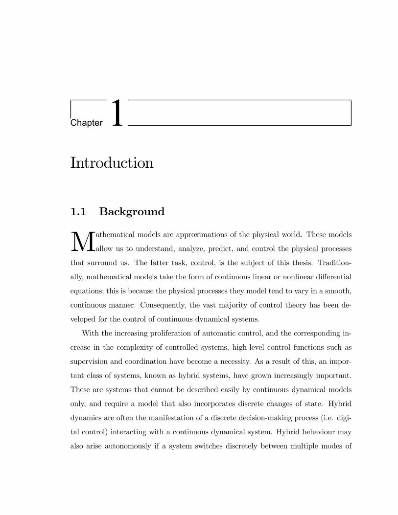
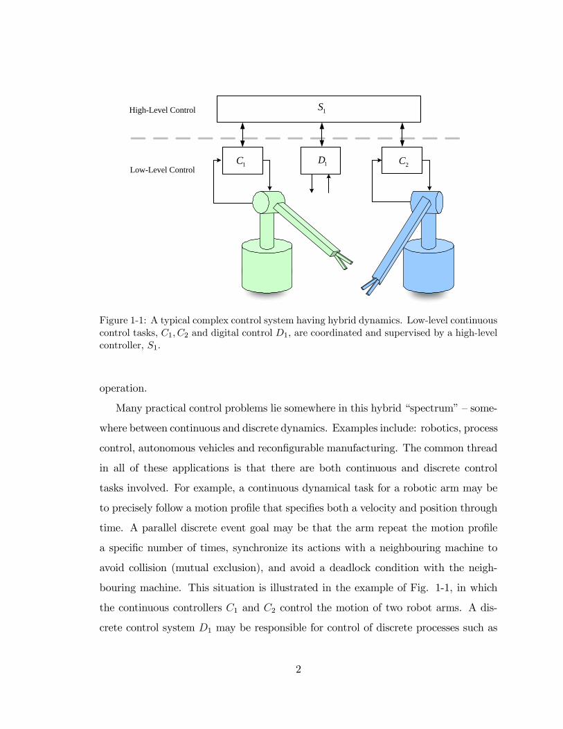
Figure 1-1: A typical complex control system having hybrid dynamics. Low-level continuouscontrol tasks, C1; C2 and digital control D1, are coordinated and supervised by a high-levelcontroller, S1.
operation.
Many practical control problems lie somewhere in this hybrid �spectrum��some-
where between continuous and discrete dynamics. Examples include: robotics, process
control, autonomous vehicles and recon�gurable manufacturing. The common thread
in all of these applications is that there are both continuous and discrete control
tasks involved. For example, a continuous dynamical task for a robotic arm may be
to precisely follow a motion pro�le that speci�es both a velocity and position through
time. A parallel discrete event goal may be that the arm repeat the motion pro�le
a speci�c number of times, synchronize its actions with a neighbouring machine to
avoid collision (mutual exclusion), and avoid a deadlock condition with the neigh-
bouring machine. This situation is illustrated in the example of Fig. 1-1, in which
the continuous controllers C1 and C2 control the motion of two robot arms. A dis-
crete control system D1 may be responsible for control of discrete processes such as
2
opening or closing valves. The supervisory controller S1 must coordinate and enforce
certain behaviours amongst the low-level systems. The mixture of discrete and con-
tinuous dynamics makes this a hybrid system. Now suppose the robots are handling
a hazardous material that cannot be dropped: this adds a safety-critical aspect to
the control task, focusing the need for formalized control design procedures that can
be proven to be safe, or error-free.
1.2 Problem Discussion
The modeling, analysis and control of hybrid systems is an open and active area of
research. The intent of this research is to develop theory and techniques that can be
applied by control system practitioners. As control system designers, the objective
is to design provably safe controllers for hybrid systems such as the one described
above. In the domain of discrete-event systems, it is possible to exhaustively search
very large system state spaces, removing trajectories that lead to unsafe states. And,
in the continuous systems domain, it is possible to ensure the stability of controlled
systems under a variety of disturbances and uncertainties. Finding a balance between
these two disparate, but mutually desirable approaches to hybrid system control is
the task at hand. Exhaustive reachability of hybrid state spaces is in general, not
possible, due to the uncountable state space. Likewise, input-to-state, and input-to-
output stabilization is problematic for even the most simple hybrid systems. The
current approaches to the hybrid design problem involve various combinations of
continuous and discrete-event modeling, simulation and analysis strategies. In either
case, the usual approach is to place more emphasis on one or the other of the types of
dynamics; e.g. approximated continuous dynamics combined with discrete switching,
or abstracted switching combined with higher-�delity continuous models. At this
time, hybrid analytical and synthesis tools are at a primitive state in comparison to
the tools of typical industrial practice. A detailed survey of the theoretical results
3
for automatic control systems in general, and hybrid systems in particular, is given
in Chapter 2. Even if the serious theoretical hurdles of hybrid system control can be
reasonably dealt with, a major barrier to adoption of hybrid control system design
techniques remains: design tools must be user-friendly and have su¢ cient utility that
designers will choose to use them. Simulation is currently the most widely utilized
technique for hybrid control system design. Controllers are simulated in many �ad-
hoc�test scenarios to identify and correct failure points in the design. This approach
relies on heuristics � the designer�s skill, and knowledge of the system, to ensure
safety.
1.3 Contributions
To solve the problem described in the previous section, it was necessary to take an
approach that was balanced between theoretical and practical considerations. This
thesis documents the technique and supporting theory that enables the automated
synthesis of supervisory controllers for systems with hybrid dynamics. The contribu-
tions are as follows:
Modeling The modeling framework developed in this thesis accommodates embed-
ded continuous simulations, thus enabling control system designers to utilize
existing simulation tools. The model, which is based on discrete switching of
continuous dynamics, is simple to use and is very expressive for capturing hybrid
dynamics. These features are an important step towards gaining acceptance of
this technique in industry.
Control Synthesis The controller synthesis technique described in this thesis uses
a hybrid system plant model and a discrete event speci�cation to produce a
discrete event supervisory controller that is safe by design. Because the con-
troller is implemented online, it can accommodate time-varying plants, and has
reduced computational complexity compared to o ine controllers, since it is
4
computed on a limited horizon. This controller can be guaranteed to be safe
(i.e. failsafe) always, by inclusion of emergency shutdown states, allowing this
technique to be utilized in safety-critical applications.
Computation A software package called HySynth was developed that implements
the control theory concepts of this thesis. The software can be used to model,
design, synthesize, and simulate online discrete event supervisory controllers,
and it helps to demonstrate the various contributions of this thesis including:
automated control synthesis for hybrid systems, online operation, failsafe con-
trol, embedded simulation, controller complexity reduction, and human in the
loop control.
Application The ship control application presented in this thesis marks the �rst
time that hybrid system control synthesis techniques have been described for
control of marine vessels. This controller is unique in that it is suited to the
incorporation of human in the loop control. This inclusion of the human op-
erator may make this control technique more attractive to implement from an
operational and liability standpoint.
1.4 Organization
This document is organized as follows: Chapter 2 contains a review of the litera-
ture that is relevant to the topics of discrete event and hybrid systems modeling,
simulation and control. Chapter 3 develops a general continuous system modeling
framework. Particular attention is paid to the partitioning framework that will be
used to produce the discrete abstractions of the continuous dynamics. Chapter 4
introduces the switched continuous model framework, and its discrete graph repre-
sentation, the hybrid transition graph. In Chapter 5 there is brief review of discrete
event controller synthesis. Developed next is the theory to support synthesis of a
fail-safe discrete-event controller for a hybrid system. This is based on the synchro-
5
nization of a switched continuous model of the plant with a discrete event model of a
speci�cation. Chapter 6 is an overview of the computational framework that is used
to support the modeling, design and online controller synthesis. Chapter 7 examines
two applications of the theory; the �rst is a benchmark hybrid control problem. This
simple example serves to illustrate the modeling environment, and through simula-
tion, gives benchmark run time complexity results. The second example demonstrates
the control design process for a realistic, industrial control problem. It also illustrates
the capacity of the control framework to incorporate heuristics (i.e. human-in-the-
loop) control. Finally, Chapter 8 again summarizes the contributions that this thesis
makes to hybrid control systems research, and suggests directions for future work.
6

Chapter2Background and Related Work
This thesis is concerned with the control of complex dynamical systems in real
time. As such, the background material contained in this chapter is of a diverse
nature, encompassing elements of control system design and applications, continuous
control system theory, discrete event control theory, hybrid system theory, and the
modeling, analysis and simulation of these systems. This chapter is a brief overview
of the models, methods and theory developed to support control system design and
analysis in these areas, and which are relevant to the results of this thesis.
2.1 Continuous System Modeling and Control
Continuous system modeling has been the dominant paradigm for theoretical and
practical developments in control systems during the 20th century. Initially, con-
trollers themselves were mechanical, then electromechanical and �nally electronic
(excluding the actuators) (Michel 1996). The "classical era" in control theory and
practice was developed around frequency domain stability techniques combined with
transient response performance analysis. Control system models were based on lin-
ear time invariant (LTI) models in a single input/single output (SISO) modeling
framework, and control design practitioners had many semi-automated procedures
7
for synthesizing controllers. Many of these techniques were developed by practicing
engineers and the theoretical explanations followed afterwards (Bernstein 2002).
With the advent of the 1960s came the state-space modeling approach of the
so-called �modern era�and the ability to model, analyze and design controllers for
multivariable or multiple input multiple output (MIMO) systems. The fundamental
concepts of state controllability and observability were formally identi�ed by Kalman
(Kalman 1960). The state space approach lends itself well to algorithmic (and hence
digital computer) implementation. Given an LTI plant model, a Linear Quadratic
Gaussian (LQG) controller can be synthesized for the system that is optimal in a
least squares sense. Furthermore, the controller is formulated for a stochastically
disturbed modeling and measurement environment, so it lends itself well to practical
application. In fact, the optimal estimator (the Kalman �lter) is widely credited with
making possible the �rst lunar landing of 1969 (p.14 (Grewal and Andrews 1993)).
Initially, there were serious drawbacks with the state-space approach since there
was no way to specify stability; and modeling errors could lead to control instability.
With H1 control design (Francis, Henton and Zames 1984), the frequency domain
approach of the classical control design techniques and notions of input to output
stability were developed for multivariable systems; see (Skogestad and Postelthwaite
1993) for an overview. Multivariable control design was further extended to include
controller robustness to parametric and structured modeling uncertainty with the
advent of �-synthesis techniques (Williams 1990), (Balas and Packard 1996).
Up to this point we have been dealing with linear system models. With nonlinear
system models, the familiar control system tools no longer apply. Nonlinear models
exhibit certain phenomena that do not arise in linear systems, including �nite escape
time, multiple equilibria, limit cycles, deterministic chaotic behaviour, and multiple
modes of operation (Khalil 2002). Typically the approach is to linearize the nonlinear
system model about some operating point, if this is possible, in order to use the
familiar and powerful linear system tools. Unfortunately, there are many classes of
8

system for which the locally linearized approximate model cannot be used; e.g. this
situation might exist if a system by necessity has more than one operating point. For
systems like this, gain scheduling (Leith and Leithead 2000) and sliding mode control
techniques have seen extensive use in industry (Kaynak, Erbatur and Ertugrul 2001).
2.2 Discrete Event Systems
Discrete event dynamical systems (DES) are characterized by having a state space
that is a discrete set and a state transition mechanism that is event driven. Usually
DES models take the form of automata or petri nets. Supervisory control theory for
DES was developed by Ramadge and Wonham, (Ramadge and Wonham 1987) and
(Wonham and Ramadge 1987). Aspects of control that are not possible to specify in
the traditional continuous control theory, such as the ordering of events, coordination
of multiple processes and enforcement of safety properties became possible with this
technique. Speci�cation and plant are both DES and modeled as �nite state automata
(FSA). Large models can be conveniently constructed by synchronous composition of
multiple FSA. Control optimality is achieved by designing a controller that minimizes
interference with the plant (minimizing plant event disablement), while enforcing the
speci�cation.
Many extensions to the basic supervisory control theory have been developed in-
cluding limited observation (Lin and Wonham 1988), decentralized supervisory con-
trol (Rudie and Wonham 1992), and robustness (Bourdon, Lawford and Wonham
2005). While technically DES have no sense of time, since they are event driven, by
addition of integer clocks and special event called tick, speci�cations and plant models
can incorporate coarse timing (O�Young 1991) and (Brandin and Wonham 1992).
DES supervisory controllers are amenable to automated computation, and a num-
ber of educational and academic packages have been developed for supervisory con-
troller design, including TTCT (Meder 1997), OTCT (O�Young 1992), and UMDES
9
(UMDES Software Library 2006), which has recently added a graphical user interface.
More detail on DES supervisory control is given in Appendix D; and for a thorough
treatment of DES modeling and supervisory control theory, refer to (Cassandras and
Lafortune 1999) and (Kumar and Garg 1995).
2.3 Hybrid System Modeling
An early hybrid system model was proposed by Witsenhausen (Witsenhausen 1966),
baring a striking resemblance to the de�nition used today. A hybrid system was
described as:
�A class of continuous time systems with part continuous, part dis-
crete state is described by di¤erential equations combined with multistable
elements.�
With any hybrid model, the goal is to capture the mixture of continuous and
discrete dynamics that are the characteristic of what we know today as hybrid sys-
tems. Generally speaking, the various hybrid models di¤er primarily in their intended
purpose and in the expressiveness of the continuous dynamics that are admitted by
the model. Furthermore, hybrid modeling tools re�ect the community from which
they arise; we divide these into the computer science community and the control
engineering community. In general, the computer science community�s approach has
been centered around proving correctness of a system with respect to a given spec-
i�cation (veri�cation), while the controls community seeks parallels to traditional
control system theory, such as stability, controllability and observability. The mod-
eling paradigms for computer science have traditionally centered around automaton
based methods, while those of the controls community have centered around switched
systems. This being said, there is considerable overlap between these communities;
each have made signi�cant contributions to the understanding of hybrid systems and
the control of hybrid systems.
10
We now examine some hybrid system models.
2.3.1 Timed Automata
The abstraction level of the coarse-timed FSM lacks the desired timing expressiveness
that is necessary for real-time control. The abstraction of the discrete-time DES su-
pervisory control approach is deemed to be unsuitable when reasoning about systems
that act (or react) directly with physical processes. The (dense) timed automaton
of (Alur and Dill 1994) is a �nite state automaton having a �nite set of real-valued
clocks. These clocks may be reset to zero upon the state transitions of the automaton
in order to keep track of time between events. Timed automata theory allows for
algorithmic analysis and veri�cation of real time systems (Alur, Courcoubetis and
Dill 1993). This approach proves useful when performing model checking on systems
that are naturally speci�ed as elapsed times, or time delays. Dense time models are
still essentially an abstraction of the underlying physical processes (i.e. continuous
variables) that give rise to the discrete events.
Automatic veri�cation tools have been developed for this class of system, no-
tably UPPAAL (Bengtsson, Larsen, Larsson, Pettersson and Yi 1995) and KRO-
NOS (Bozga, Daws, Maler, Olivero, Tripakis and Yovine 1998). These packages have
both been applied to the veri�cation of communication protocols; problems that con-
tain �hard�timing constraints (Daws, Kwiatkowska and Norman 2004) (David and
Yi 2000). However, owing to the complexity of these protocols, these examples have
been carried out only on some portion of the protocol, and were formulated with
simpli�ed models of the protocol software code.
2.3.2 Hybrid Automata
This is a �nite state graph, in which each state has some continuous dynamics (not
necessarily constant rate) speci�ed as di¤erential equations. The switching between
states is instantaneous and is governed by guards (or invariants) based on the con-
11

tinuous variables (Henzinger and Ho 1995). The hybrid automaton is an intuitive
and expressive model since it uses the familiar �nite state automaton paradigm. An
execution of a hybrid model then consists of the continuous states varying according
to the currently speci�ed dynamics, followed by a discrete jump to a new state and
so on. A natural extension of the timed automaton is the so-called �linear�hybrid
automaton (Henzinger 2000), a special case of hybrid automaton that requires the
continuous dynamics to be constant rate. Essentially, the LHA is a special case of
a timed automaton in which the clocks may run at di¤erent rates with respect to
each other. This extension of the timed automaton takes the model one step closer
to the physical variables, since now the variable rate clocks may model a variety of
real-valued continuous variables instead of time.
In general however, the algorithmic veri�cation of the hybrid automaton models
is undecidable, since model checking is based ultimately on computing the reachabil-
ity of an in�nite state space. Algorithmic veri�cation of system properties for LHAs
are only semi-decidable. When the model is based on a special sub-classes of the
linear hybrid automaton; i.e. the rectangular automaton, veri�cation is known to
be decidable (Henzinger, Kopke, Puri and Varaiya 1998). A software package that
implements hybrid system veri�cation for LHAs called HyTech (Henzinger, Ho and
Wong-Toi 1997), (Henzinger, Ho and Wong-Toi 1996) was developed and has found
considerable use primarily as a teaching tool and for academic research. HyTech has
been reportedly used to verify and parameterize properties in a variety of simpli-
�ed applications including (to name a few), a steam boiler control (Henzinger and
Wong-Toi 1995b), a distributed sensor network (Coleri, Ergen and Koo 2002), ship
coordination and control system (Millan and O�Young 2000) and a pneumatic au-
tomotive suspension control system (T. Stauner, O. Mueller and M. Fuchs 1997).
Unfortunately, the main shortcoming of these applications is that the nonlinear con-
tinuous dynamics must be approximated by constant rate dynamics (Henzinger and
Wong-Toi 1995a). If a system is meant to be safety critical, then incorrect approx-
12
imation of the nonlinear dynamics could lead to safety violations. Furthermore, for
the control examples, HyTech assumes that a controller exists already for the hybrid
system; it veri�es the design or parameterizes it; in general designing the controller
for a complex system is an important part of the problem.
The hybrid I/O automaton (HIOA) framework was intended to support descrip-
tion and analysis of hybrid systems, adding a complex input/output interface to the
basic HA (Lynch, Segala and Vaandrager 2003). Composition operations amongst
HIOA models accommodate more complex modeling of hybrid systems. Unfortu-
nately there is no computational tool to support this modeling framework, so the com-
position and veri�cation is carried out by hand using mathematical proofs thus lim-
iting applications to simple laboratory-based demonstrations (Fehnker, Vaandrager
and Zhang 2003) and (Mitra, Wang, Lynch and Feron 2003).
2.3.3 Quantized I/O (Discrete Event Abstraction)
Another approach to hybrid systems modeling has centered around discrete abstrac-
tions of continuous systems. This approach is characterized by a control theoretical
approach, centered around leveraging the �correct-by-design�results of DES supervi-
sory control theory. In (Raisch and O�Young 1998), discrete abstractions based on the
truncated time history of discrete-time LTI continuous models were used to synthesize
DES supervisory controllers. In a behavioural sense, if the behaviour of the discrete
abstraction contains that of the continuous system, then the safety properties of a
DES controller based on the abstraction are ensured (Raisch 2000), (Moor, Raisch
and Davoren 2001). The controller is a discrete-event controller, while the plant ex-
ists in the continuous domain, so from an I/O point of view, there are A/D and
D/A interfaces between the two (Lemmon, He and Markovsky 1999), (Koutsoukos,
Antsaklis, Stiver and Lemmon 2000). In (Su, Abdelwahed, Karsai and Biswas 2003),
(Abdelwahed, Su and Neema 2005), discrete abstractions of continuous dynamics
were adapted in a limited horizon to synthesize DES supervisors.
13
2.3.4 Switched Systems
Many approaches to hybrid modeling fall into the category of switched systems. The
switched system approach is characterized by the high �delity modeling of the continu-
ous dynamics, with less attention paid to the logic; these are generally non-automaton
based representations of hybrid systems.
The emphasis of the switched system approach to hybrid systems is primarily on
control system stability and optimality. Typically there are a collection of continuous
system dynamics amongst which a controller may switch; conditions are sought under
which the switched (or hybrid) system is stable. Worth noting is the fact that even if
each individual system is stable, unconstrained switching may actually destabilize the
overall system. Conversely, switching may be used to stabilize the overall system even
if the individual subsystems are themselves unstable (Hespanha and Morse 2002). For
arbitrary switching by the supervisory controller, the hybrid system will be stable if a
common Lyapunov function can be found for each of the continuous dynamics. Under
state based switching conditions, stability may be guaranteed if multiple Lyapunov
functions can be found for each of the switched systems (Branicky 1998).
Many special subclasses of switched system models have been proposed that use
approximated continuous dynamics to achieve improved computational complexity
at the expense of veri�cation and control conservatism. These models include mixed
logical dynamical (MLD), piecewise a¢ ne (PWA) and others; each has been shown
to be input-state-output equivalent under certain assumptions (Heemels, de Schutter
and Bemporad 2001). Closed loop model predictive control (MPC) has also been
shown to be equivalent to these other forms of linear switched systems under cer-
tain assumptions (Bemporad, Heemels and de Schutter 2002), meaning that switched
system results can also be applied to MPC by translating them into MLD or PWA
problems.
Software has been developed for analyzing, simulating and even synthesizing con-
trollers for systems modeled by PWA and MLD models (Torrisi and Bemporad 2004),
14
(Torrisi and Bemporad 2001) in discrete time. Based on the package HYSDEL (Hy-
brid Description Language) and implemented in the MatlabR /Simulink
R environ-
ment, PWA models can be interfaced to �nite state automata. The software is capa-
ble of generating linear and hybrid MPC (receding horizon) control laws in piecewise
a¢ ne form. Another software tool, CheckMate, has been developed in the Mat-
lab/Simulink environment for hybrid system veri�cation (Chutinan and Krogh 2003).
Beginning with a polyhedral set of initial continuous states and continuous ranges of
parameter values, this package can verify that all trajectories of the model meet some
speci�cation.
Typical applications that have been looked at are synthesizing an engine idle speed
controller (Balluchi, Natale, Sangiovanni-Vincentelli and van Schuppen 2004) using
PWA hybrid models, air tra¢ c control routing problem optimized by using mixed
integer linear programming (MILP) (Bayen and Tomlin 2003) and a chemical batch
processing system using PWA and MLP (Potocnik, Bemporad, Torrisi, Music and
Zupancic 2004). A survey of automotive applications of the switched system control
approach are contained in (Balluchi, Benvenuti and Sangiovanni-Vincentelli 2005).
General references for switched systems control and stability can be found in
(Liberzon 2003), (Hespanha 2004), and for a short overview, see (Lin and Antsaklis
2005).
2.4 Hybrid System Simulation
When designing control systems for hybrid systems, simulation is without a doubt
the most heavily utilized tool by designers. Typically, controllers are tested under
a variety of conditions by simulation to evaluate the safety and correctness of a
particular design. However, due to the ad-hoc choice of these test conditions, this
technique may miss the particular combination of conditions that leads to design
failure. In spite of this, hybrid simulation is still an important tool.
15
The statechart modeling formalism was originally developed by (Harel 1987) to en-
capsulate the notions of hierarchy, concurrency, and communication for discrete event
system models. Statecharts have been widely used and were subsequently extended to
include continuous dynamics; an example of a commercial simulation tool using stat-
echarts is the Matlab StateFlowR toolbox for Simulink . Various packages have also
been developed for academic use, including CHARON (Alur, Dang, Esposito, Hur,
Ivancic, Kumar, Lee, Mishra, Pappas and Sokolsky 2003) a language for describing
hybrid and timed systems. Ptolemy is a general-purpose modeling package with a
graphical user interface (Lee 2003). HyVisual, based on Ptolemy, is also a visual mod-
eling package, but is designed speci�cally to model hybrid systems (Brooks, Cataldo,
Lee, Liu, Liu, Neuendor¤er and Zheng 2005). HyBrSim is an object-oriented hybrid
simulation tool based on bond graph models of hybrid systems (Mosterman 2002).
Another hierarchical hybrid simulation tool called YAHMST (Yet Another Hybrid
Modeling and Simulation Tool) has also been reported (Thevenon and Flaus 2000).
A comprehensive overview of these and other hybrid modeling, simulation and
veri�cation tools is given in (Carloni, DiBenedetto, Pinto and Sangiovanni-Vincentelli
2004).
2.5 Complexity
A common thread in the control problems formulated with the models presented
here is that most are either undecidable or computationally intractable (Blondel and
Tsitsiklis 2000). Undecidable problems are ones for which a suitable algorithm cannot
be constructed to: a) terminate, and b) return a correct answer. Computationally
intractable problems are considered to be those for which a polynomial-time algorithm
cannot be found, and thus they are not amenable to computation; these are known
as NP-hard problems.
It has been shown for simple hybrid systems consisting of switched continuous
16
systems that verifying properties such as stability and controllability are either unde-
cidable or NP-hard (Blondel and Tsitsiklis 1999). Veri�cation of properties for sys-
tems modeled by simple linear hybrid automata (and even for some timed automata),
have been shown to be undecidable (Henzinger et al. 1998). In DES supervisory con-
trol, the modular supervisor control synthesis is NP-hard due to the familiar �state
explosion�problem (Gohari and Wonham 2000). Even in the area of robust control,
the calculation of the structured singular value �, has been shown to be NP-hard
(Braatz, Young, Doyle and Morari 1994).
Clearly, the quest for veri�cation and optimality in �real�hybrid or DES control
problems is unlikely to be successful. Hence, control solutions will likely have to be
sub-optimal or ��t for purpose�, and thus new control theory has to be driven by the
applications.
2.6 Assessment of Relevant Work
The work presented in this thesis is inspired by the industrial control problems encoun-
tered with the safety critical control and coordination and manoeuvring of multiple
marine vessels. Practicing controls engineers need design techniques and tools that
are easy to use and understand.
2.6.1 Model Formulation
The switched continuous model (SCM) that is developed in Chapter 4 is a blend of
the switched system and discrete abstraction approaches to hybrid modeling. We
use a �exible state space partitioning based on continuously di¤erentiable functionals
as in (Koutsoukos et al. 2000). However, instead of switching piecewise constant
inputs, we switch the entire continuous dynamic as is done in the switched system
approach. This admits a very expressive continuous modeling to be utilized. The
vast majority of switched system approaches emphasize global stability or optimality,
17
and therefore must use linear approximations of continuous dynamics in order to
make the computation more tractable. Because we use a �nite time horizon, we can
relax the goal of stability, which is traditionally de�ned on in�nite time. In addition,
because we deal with a discrete abstraction, optimality is relaxed to merely a safety
requirement in the sense of state avoidance. These tradeo¤s permit us to admit a
larger class of nonlinear continuous dynamics (Millan and O�Young 2006a).
2.6.2 Discrete Abstraction
Previous discrete abstraction work has focussed on obtaining a single o ine discrete
event model, with the added requirement that the model be deterministic. This desire
leads to state space partitioning regimes that attempt to match the �ow of the contin-
uous dynamics (Koutsoukos and Antsaklis 2001). In (Su et al. 2003), the partitioning
is based on re�nements of polyhedral partitions until the model�s nondeterminism
is reduced to some satisfactory measure. Since our technique involves abstracting
the model repeatedly in an online fashion, no single discrete abstraction is required.
And having full-state information, a deterministic model is not required, since we
have cast our DES supervisor synthesis as a state avoidance problem. As a result,
the main consideration of the partitioning is to generate discrete events (symbols) in
order to synchronize with other processes that make up the plant or speci�cation.
Furthermore, (Raisch and O�Young 1998) showed that enforcing safety of the dis-
crete abstraction guarantees the safety of the corresponding continuous model if the
discrete abstraction is a conservative approximation of the continuous model.
2.6.3 Controller Synthesis
Similar to our work is (Stursberg 2004), in which the nonlinear continuous dynamics
are retained as embedded simulations. Working with a �nite set of control actions,
an acyclic graph branching in discrete time intervals, with hybrid nodes (states) is
constructed. The search of this graph is steered by optimality constraints using a
18
combination of depth and breadth �rst reachability. Our technique di¤ers in that we
construct a �nite state graph which is pruned in a maximally permissive sense with
respect to a safety speci�cation, in accordance with optimal DES supervisory control
theory. Furthermore, our approach admits both state and time dependent switching
of dynamics.
2.6.4 Computation
In the work of (Stursberg, Fehnker, Han and Krogh 2003), it was noted that a re-
duction in computational complexity may be realized by including the speci�cation
when calculating reachable sets for hybrid veri�cation problems. Most hybrid reach
set computations simply expand the reach set incrementally in all directions without
regard to the speci�cation. In our controller synthesis technique, the inclusion of the
speci�cation during synthesis allows for a reduction in computational complexity due
to the fact that illegal traces may be eliminated as soon as an illegal state is reached;
i.e. before it is added to the reach set.
We utilize a limited lookahead scheme similar to that initially explored in (Chung,
Lafortune and Lin 1992), in which DES supervisors are computed for a limited looka-
head event horizon. This technique was intended to reduce computational complexity
for DES control synthesis and to allow time-varying plants to be handled, since it is an
online technique. In limited lookahead control, safety and nonblocking properties can
only be guaranteed by adopting a conservative approach with regard to the extension
of traces beyond the lookahead horizon; that is, they assume that all traces continue
to unsafe or blocking states. Our approach is also conservative, and we de�ne the
notion of emergency shutdown states, specially marked states to ensure system safety
(Millan and O�Young 2006b).
In (Giorgetti, Pappas and Bemporad 2005), a �nite-time discrete transition system
is extracted from the linear continuous dynamics of a discrete-time hybrid automaton
(DHA) model on a limited horizon. A technique known as bounded model checking
19
(BMC) is then used to verify the system against a speci�cation, which is expressed
as a temporal logic formula. Instead of verifying a controller design, as in this o ine
approach , we repeatedly construct controllers online by the synchronous product
connection of the plant and speci�cation. Our �nite state graph (called a hybrid
transition graph) represents the controller and is correct by design because it repre-
sents the (exhaustive) reachable state space, on a limited horizon, of the plant pruned
by a safety speci�cation.
2.7 Summary
In this chapter we have examined some common approaches to hybrid system mod-
eling that have been reported in the literature. The various techniques and tools for
simulation, veri�cation, and control synthesis have developed from two communities
with backgrounds of control systems (electrical engineering) and computer science.
Both of these research approaches have had some successes, but no hybrid system
control techniques have yet seen any widespread acceptance by industry. Simulation
still seems to be the dominant approach to hybrid system control design. The promise
of the de�nitive veri�cation, optimality and provably stable hybrid system controller
appears to be an elusive goal; many of these have been shown to be either undecidable
problems or computationally intractable.
A comparison of the techniques developed in this thesis with those of the literature
has been presented. In the following chapters, these modeling and computational and
control synthesis techniques are developed in further detail.
20

Chapter3Abstraction of Continuous System
Dynamics
3.1 Introduction
The goal of this chapter is to develop a discrete event abstraction of a continuous
model that ultimately will be suitable for discrete event supervisory control.
The approach taken is to select a natural and expressive continuous modeling frame-
work and then to overlay it with a discrete event, input/output (I/O) interface. For
now, we consider the output aspects of the interface, or the conversion of the contin-
uous dynamics to that of discrete event dynamics.
The continuous dynamics of a system may be described by a nonlinear ordinary
di¤erential equation (ODE),
_x(t) = f(x; t) (3.1)
In general, the objective of the discrete abstraction is to achieve a single, preferably
deterministic, automaton representation of the continuous dynamics. Based on this
discrete abstraction, standard DES supervisory control techniques can be used to
develop a DES controller. The discrete abstraction is intended to capture only the
important dynamics (those that matter to the DES controller), thereby reducing the
21
),( txfx =ɺ
Interface LayerAbstraction:
State QuantizationDiscrete Event
Generation)(tx *s ∈Σ
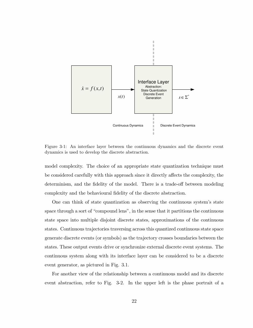
Continuous Dynamics Discrete Event Dynamics
Figure 3-1: An interface layer between the continuous dynamics and the discrete eventdynamics is used to develop the discrete abstraction.
model complexity. The choice of an appropriate state quantization technique must
be considered carefully with this approach since it directly a¤ects the complexity, the
determinism, and the �delity of the model. There is a trade-o¤ between modeling
complexity and the behavioural �delity of the discrete abstraction.
One can think of state quantization as observing the continuous system�s state
space through a sort of �compound lens�, in the sense that it partitions the continuous
state space into multiple disjoint discrete states, approximations of the continuous
states. Continuous trajectories traversing across this quantized continuous state space
generate discrete events (or symbols) as the trajectory crosses boundaries between the
states. These output events drive or synchronize external discrete event systems. The
continuous system along with its interface layer can be considered to be a discrete
event generator, as pictured in Fig. 3.1.
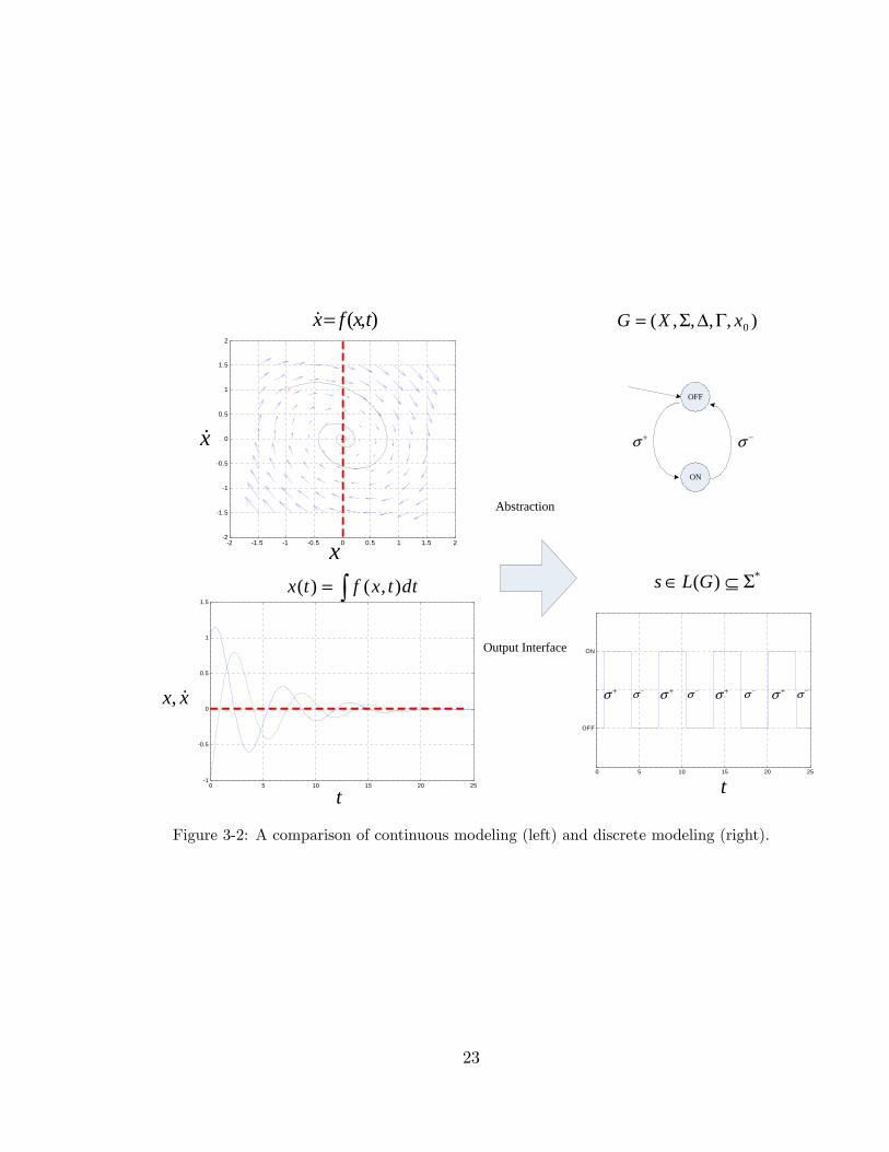
For another view of the relationship between a continuous model and its discrete
event abstraction, refer to Fig. 3-2. In the upper left is the phase portrait of a
22
0 5 10 15 20 25
OFF
ON
0 5 10 15 20 25-1
-0.5
0
0.5
1
1.5
-2 -1.5 -1 -0.5 0 0.5 1 1.5 2-2
-1.5
-1
-0.5
0
0.5
1
1.5
2
( , )x f x t=� ),,,,( 0xXG Γ∆Σ=
*)( Σ⊆∈ GLs( ) ( , )x t f x t dt= ∫
Abstraction
Output Interface
σ −σ + σ + σ +σ −σ + σ − σ −
OFF
σ + σ −
ON
x
x�
,x x�
t t
Figure 3-2: A comparison of continuous modeling (left) and discrete modeling (right).
23

continuous system, essentially a graphical representation of the continuous dynamics
of a modeled system (Eq. 3.1). Superimposed on the phase portrait is a trajectory
x(t), the continuous behaviour, and the phase plane has been partitioned into two
regions. In the lower left, the state variables of x(t) are plotted against time. The
upper right of the diagram is the graphical representation of the DES model of the
same continuous system, a �nite state machine graph. In the lower right, the dis-
crete event behaviour of the FSM for the same continuous trajectory. Comparisons
may be drawn between the continuous state space approach and its counterpart, the
automaton representation. Likewise, there is a parallel between the continuous in-
put/output model and languages of automata (Boel, Cao, Cohen, Giua, Wonham and
van Schuppen 2002).
A discrete abstraction of a continuous model is de�ned by the state quantization
and the event generation processes. This chapter examines the discrete abstraction of
a generalized continuous model on a �nite time horizon. The discrete abstraction of
the continuous system can be viewed as an autonomous generator of discrete events.
In this context, we examine one particular state abstraction technique that utilizes
continuous functionals to partition the state space of a given system model. This
technique was developed extensively in (Stiver, Koutsoukos and Antsaklis 2000) and
(Koutsoukos et al. 2000). In these works, functionals F : Rn ! R are used to partition
the state space of a continuous system. For purposes of supervisory control, the null
space of these functionals are designed to be invariant manifolds with respect to the
vector �eld of the continuous dynamics. The resulting partitions have common entry
and exit boundaries, thus permitting deterministic DES models to be extracted.
In this chapter, we expand on the work of (Koutsoukos et al. 2000) by develop-
ing bounds on the cardinality of the state label set and event label set of a discrete
abstraction due to a general family of partitioning functionals. We relax the require-
ment that the resulting partitions be invariant with respect to the continuous �ow
�eld, since without loss of generality, we do not require a deterministic DES model.
24
The emphasis is to develop a practical and �exible mechanism for obtaining discrete
abstractions of continuous dynamical systems, from which an algorithmic implemen-
tation can be developed. Finally, this chapter outlines the conditions that will be
required for a generalized discrete abstraction in the following chapters.
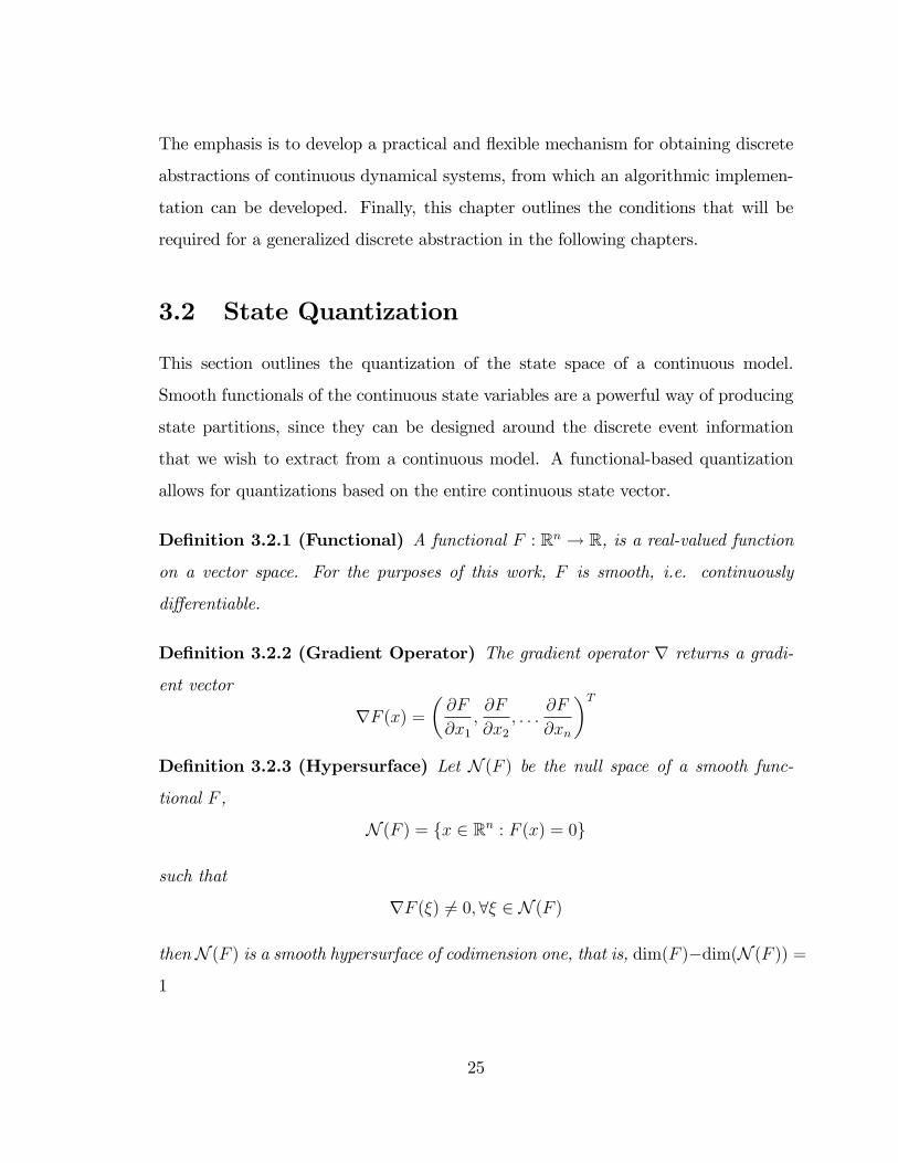
3.2 State Quantization
This section outlines the quantization of the state space of a continuous model.
Smooth functionals of the continuous state variables are a powerful way of producing
state partitions, since they can be designed around the discrete event information
that we wish to extract from a continuous model. A functional-based quantization
allows for quantizations based on the entire continuous state vector.
De�nition 3.2.1 (Functional) A functional F : Rn ! R, is a real-valued function
on a vector space. For the purposes of this work, F is smooth, i.e. continuously
di¤erentiable.
De�nition 3.2.2 (Gradient Operator) The gradient operator r returns a gradi-
ent vector
rF (x) =�@F
@x1;@F
@x2; : : :
@F
@xn
�TDe�nition 3.2.3 (Hypersurface) Let N (F ) be the null space of a smooth func-
tional F ,
N (F ) = fx 2 Rn : F (x) = 0g
such that
rF (�) 6= 0;8� 2 N (F )
thenN (F ) is a smooth hypersurface of codimension one, that is, dim(F )�dim(N (F )) =
1
25
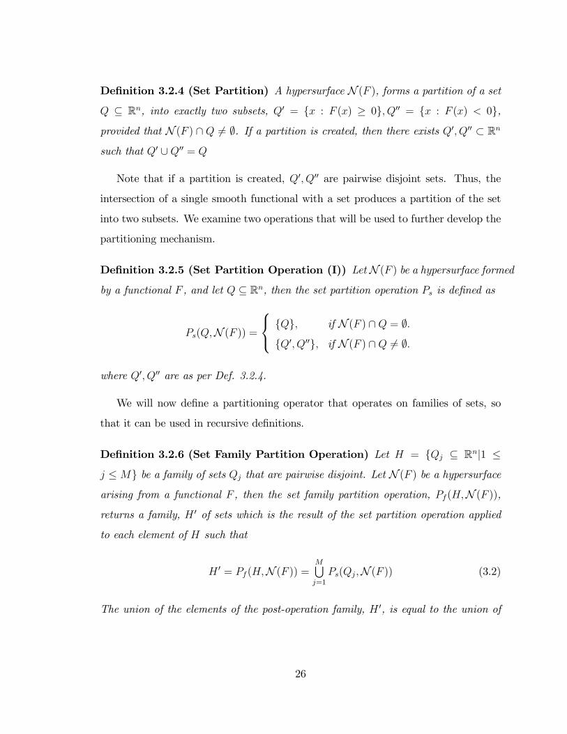
De�nition 3.2.4 (Set Partition) A hypersurface N (F ), forms a partition of a set
Q � Rn, into exactly two subsets, Q0 = fx : F (x) � 0g; Q00 = fx : F (x) < 0g,
provided that N (F ) \ Q 6= ;. If a partition is created, then there exists Q0; Q00 � Rn
such that Q0 [Q00 = Q
Note that if a partition is created, Q0; Q00 are pairwise disjoint sets. Thus, the
intersection of a single smooth functional with a set produces a partition of the set
into two subsets. We examine two operations that will be used to further develop the
partitioning mechanism.
De�nition 3.2.5 (Set Partition Operation (I)) LetN (F ) be a hypersurface formed
by a functional F , and let Q � Rn, then the set partition operation Ps is de�ned as
Ps(Q;N (F )) =
8<: fQg; if N (F ) \Q = ;:
fQ0; Q00g; if N (F ) \Q 6= ;:
where Q0; Q00 are as per Def. 3.2.4.
We will now de�ne a partitioning operator that operates on families of sets, so
that it can be used in recursive de�nitions.
De�nition 3.2.6 (Set Family Partition Operation) Let H = fQj � Rnj1 �
j �Mg be a family of sets Qj that are pairwise disjoint. Let N (F ) be a hypersurface
arising from a functional F , then the set family partition operation, Pf (H;N (F )),
returns a family, H 0 of sets which is the result of the set partition operation applied
to each element of H such that
H 0 = Pf (H;N (F )) =MSj=1
Ps(Qj;N (F )) (3.2)
The union of the elements of the post-operation family, H 0, is equal to the union of
26
the elements of the pre-operation family,
SQ0j2H0
Q0j =S
Qj2HQj
A simple example of the set family partitioning operation follows,
Example 3.2.1 Let H = fQ1; Q2; : : : ; QMg if for all j; Qj \N (F ) 6= ; then
H 0 = Pf (H;N (F )) = Ps(Q1;N (F )) [ Ps(Q2;N (F )) [
: : : [ Ps(QM ;N (F ))
H 0 = fQ01; Q001g [ fQ02; Q002g [ : : : [ fQ0M ; Q00Mg
= fQ01; Q001; Q02; Q002; : : : ; Q0M ; Q00Mg
NowSj
(Q0j [Q00j ) =Sj
(Qj).
Now for repetitive partitioning operations, it is necessary to prove some properties
of the set family partitioning operation.
Lemma 3.2.1 Let H = fQj � Rnj1 � j � Mg and N (F ) \ Qj = ;, 8Qj 2 H andMTj=1
Qj = ;; then the number of sets in the resulting family, jH 0j = jPf (H;N (F ))j =M
and moreover, H = H 0.
Proof. Since N (F ) \ Qj = ; for all Qj 2 H; then it follows from the de�nition
of the set family partition operation Pf (Def. 3.2.6), that
jH 0j =����� MSj=1Ps(Qj;N (F ))
�����= jPs(Q1;N (F ))j+ jPs(Q2;N (F ))j+ : : :+ jPs(QM ;N (F ))j
= 1 + 1 + : : :+ 1| {z }M
= M
27
Now for case that each partitioning operation results in a non-empty hypersurface
intersection,
Lemma 3.2.2 Let H = fQj � Rnj1 � j � Mg and N (F ) \ Qj 6= ;, 8Qj 2 H and
ifMTj=1
Qj = ; then the number of sets in the resulting family, jH 0j = jPf (H;N (F ))j =
2M .
Proof. Since N (F ) \ Qj 6= ; for all Qj 2 H; then it follows directly from the
de�nition of the set family partition operation Pf (Def. 3.2.6) that
jH 0j =����� MSj=1Ps(Qj;N (F ))
�����= jPs(Q1;N (F ))j+ jPs(Q2;N (F ))j+ : : :+ jPs(QM ;N (F ))j
= 2 + 2 + : : :+ 2| {z }M
= 2M:
A further example will illustrate the successive partitioning operations, given
Lemma 3.2.1 and Lemma 3.2.2.
Example 3.2.2 Let H = fQ1; Q2g be a family of sets and let F be a functional such
thatN (F )\Q1 6= ; andN (F )\Q2 6= ;. ThenH 0 = Sf (H;N (Fa)) = fQ01; Q001; Q02; Q002g
and jH 0j = 2 jHj = 2 � 2 = 4. Likewise, if there are no set intersections with the
hypersurface, then the operation returns the original family of sets unaltered H 0 =
Sf (H;N (Fa)) = fQ1; Q2g, i.e. jH 0j = jHj = 2.
Up to this point, only a single functional has been used to partition a single set
or family of sets. We will now look at the e¤ect a family of partitioning functionals
has upon a set, by applying the set family partitioning operator recursively
28
De�nition 3.2.7 (Set Partition Operation (II)) Let Q � Rn and let be a
family of smooth functionals, fFi : Rn ! R; 1 � i � Ng. The set family parti-
tion operator recursively partitions Q into a family of sets
H 0 = Pf (: : : Pf (Pf| {z }N times
(fQg;N (F1));N (F2)); : : : ;N (FN)) (3.3)
The entire state space of a system, Q = Rn, can be separated into a family of
subsets using the operator described in Def. 3.2.7. Given a family, ofN functionals,
fFi : Rn ! R; 1 � i � Ng the corresponding hypersurfaces, N (Fi) separate the state
space of a system into a family of sets.
How does the family of sets Q 2 H 0 relate to the discrete states of the DES model?
It can be shown that the family of partitioning functionals establishes an equivalence
relation on the system state space.
De�nition 3.2.8 (Equivalence relation) Let = fFi : Rn ! R; 1 � i � Ng be
a family of functionals de�ned on the state space of the system described by _x(t) =
f(x; t); x(t) 2 Rn, then an equivalence relation is de�ned on Rn by the partitioning
functionals
x1 �p x2 () (sign(Fi(x1))� sign(Fi(x2)) = 1; for all i, 1 � i � N) (3.4)
De�nition 3.2.9 (Equivalence Class) Each set Qj � Rn is an equivalence class
created by the equivalence relation �pof Eq. 3.4.
De�nition 3.2.10 (Quotient Set) The set of all equivalence classes X , given the
equivalence relation �p, is known as the quotient set X = Rn= �p.
The members of the quotient set are the subsets Qj resulting from a state space
partitioning operation. These subsets (or equivalence classes) will be associated with
discrete system states through a state labeling function that assigns a unique state
29
label to each of the discrete states corresponding to the subsets Qj 2 X .
De�nition 3.2.11 (Unit Step Function) We de�ne a unit step function as:
h(�) =
8<: 1 � � 0
0 � < 0
De�nition 3.2.12 (State Labeling Function) Let be a family of N functionals
partitioning a state space, then let V : Rn ! f0; 1gN , be a function that identi�es the
system state x 2 Rn with a labeling vector as follows:
V (x) =hh(F1(x)) h(F2(x)) � � � h(FN(x))
iTThus each member of the quotient set Qj 2 X is associated with a unique label
vector generated by the state labeling function.
We will establish bounds on the cardinality of the resulting family of sets due to
this state partitioning operation. Let H 0i be the ith family of sets returned by the
ith nested set family partition operation, P if (Hi;N (Fi)); then for the next recursive
operation, P i+1f , Hi+1 = H 0i. If each functional Fi intersects with only one setQj 2 Hi,
for each P if (Hi;N (Fi)) operation in Eq. 3.3 then this will be termed as minimal
intersection. Conversely, if each of the functionals, Fi intersects with all Qj 2 Hi for
each P if (Hi;N (Fi)) operation this is termed maximal intersection.
Maximal intersection determines the upper bound of cardinality resulting from
the state space partitioning operation.
Lemma 3.2.3 (State Space Partition Upper Bound) Let Q = Rn be the state
space of a system, and let = fFi : Rn ! R; 1 � i � Ng be a family of functionals.
The set partition operation (II) of Def. 3.2.7, will produce a family of sets, H 0, such
that the upper bound on the number of sets is jH 0j = 2N .
30
Proof. Proof of the upper bound is made by assuming maximal intersection and
by induction. For the (base) case of one functional N = 1, the set family partition
operation P 1f (fQg;N (F1)) reduces to the set partition operation Ps(Q;N (F )) because
there is only one set in the family H1 = fQg and only one functional. Since Q = Rn,
thus Q \ N (F1) 6= ;. It follows from Def. 3.2.5 that the cardinality of the returned
family is (by Lemma 3.2.2) jH 01j = 2N = 21 = 2. The inductive hypothesis is that
jH 0N j = 2N . It remains to show
��H 0N+1
�� = 2N+1. Suppose there exists FN+1 that hasmaximal intersection for all Qj 2 H 0
N and since by de�nition
HN+1 = H 0N
H 0N+1 = PN+1f (HN+1;N (FN+1)) =
MSj=1
Ps(Qj;N (FN+1))
Therefore,
��H 0N+1
�� =
����� MSj=1Ps(Qj;N (F ))�����
= jPs(Q1;N (FN+1))j+ jPs(Q2;N (FN+1))j+ : : :+ jPs(QM ;N (FN+1))j
= 2 + 2 : : :+ 2| {z }M
= 2M
where jH 0N j = M = 2N . It follows then that
��H 0N+1
�� = 2M = 2 � 2N = 2N+1, thus
proving the inductive hypothesis to be correct.
The lower bound of the state space partitioning operation is determined by the
minimal intersection of the partitioning functionals.
Lemma 3.2.4 (State Space Partition Lower Bound) Let Q = Rn be the state
space of a system, and let = fFi : Rn ! R; 1 � i � Ng be a family of functionals,
such that there is minimal intersection. The set partition operation (II) of Def. 3.2.7
will produce a family of sets H 0, such that the lower bound on the number of sets is
31
jH 0j = N + 1.
Proof. Prove the lower bound by induction. The base case is N = 1, or one
functional F1, so
H1 = P 1f (fQg;N (F1)) = Ps(Q;N (F1));
and clearly Q\N (F1) 6= ;, therefore jH 01j = 2 by de�nition. The inductive hypothesis
is that jH 0N j = N + 1. It remains to show that for N + 1 functionals
��H 0N+1
�� =(N +1)+ 1 = N +2. Suppose there exists FN+1 and only one set Q1 2 H 0
N (minimal
intersection), such that Q1 \ N (FN+1) 6= ; and recall that H 0N = HN+1. Then, by
de�nition
H 0N+1 = PN+1f (HN+1;N (FN+1)) =
MSj=1
Ps(Qj;N (FN+1))
where jH 0N j = jHN+1j =M = N + 1. Expanding the cardinality expression
��H 0N+1
�� =MSj=1
Ps(Qj;N (FN+1))
= jPs(Q1;N (FN+1))j+ jPs(Q2;N (FN+1))j+ : : :+ jPs(QM ;N (FN+1))j| {z }M�1 terms
= 2 + 1 + : : :+ 1| {z }M�1
= 2 +M � 1
= N + 2:
Having established upper and lower cardinality bounds on the state space parti-
tioning operation, it is possible to develop a general theorem on the range of cardi-
nality for the general result of this operation.
Theorem 3.2.1 (State Space Partition Boundedness) Let Q = Rn be the state
space of system and let = fFi : Rn ! R; 1 � i � Ng be a family of functionals,
with N �nite. Then the state space shall be partitioned into a family of sets H 0, such
32
that jH 0j is �nite and furthermore that
N + 1 � jH 0j � 2N :
Proof. Let jj = N . It follows from Lemma 3.2.4 that the cardinality of a
resulting state space partition is bounded below and is jH 0j � N + 1. Lemma 3.2.3
ensures that there is an upper bound on the cardinality of the resulting state space
partition, H � 2N+1. Hence the result follows that any �nite family of functionals
induces a �nite partition of sets on Rn.
See Appendix B for further results on set partitioning using functionals.
3.3 Discrete Event Generation
A state quantization scheme has been established using families of functionals that
produces a �nite set of discrete states and corresponding state labels. There is an
equivalence between these discrete states and subsets of the continuous state space.
We now de�ne the event generation mechanism for our discrete abstraction. To do
this, we examine in more detail the continuous trajectories crossing the state space
of the continuous model, and how these trajectories are manifested in the discrete
abstraction.
De�nition 3.3.1 (Continuous Trajectory) A continuous trajectory of a system
is de�ned as a solution x(t), to an IVP for _x = f(x; t), and an initial condition
x0 = x(t0), over some �nite time interval [t0; tf ].
A transition occurs upon the traversal of a continuous trajectory between a pair
of regions or sets. For further de�nitions and discussion of continuous solutions to
ordinary di¤erential equations, refer to Appendix A. In general, solutions of ODEs
require an assumption that the function f be Lipschitz continuous in order for the
solution to exist and be unique.
33
De�nition 3.3.2 (Transition) Let Q1,Q2 � Rn be a pair of sets such that Q1\Q2 =
;. Let x(t) 2 Rn, a solution to an IVP on time interval [t0; tf ] such that x(t) 2 Q1[Q2for all t 2 [t0; tf ]. If the continuous trajectory crosses a hypersurface, and then enters
the state, then the system is said to have undergone a transition.
9x1 = x(t1); x2 = x(t2); t1; t2 2 [t0; tf ] and t1 < t2 such that x1 2 Q1 and x2 2 Q2
The transition of a continuous trajectory from Q1 to Q2 will be indicated by the
following notation
Q1 Q2
Formally, the transition occurs at the moment when the trajectory x(t) �rst enters
the region Q2.
De�nition 3.3.3 (Discrete Event) An atomic discrete system event � is generated
when a transition occurs.
For the purpose of event timing, it is important to have a consistent de�nition of
exactly when the discrete event occurs.
De�nition 3.3.4 (Discrete Event Time) Let Q1,Q2 � Rn. Let x(t) 2 Rn be a
solution to an IVP for _x = f(x; t), and an initial condition x0 = x(t0), over some
�nite time interval [t0; tf ] such that x(t) 2 Q1 [ Q2 for all t 2 [t0; tf ]. There is a
corresponding transition, as in Def. 3.3.2. Let x0(t) 2 Q1 be the solution on the time
interval [t0; te) and let x00(t) 2 Q2 be the solution on the time interval [te; tf ]. The
atomic discrete event corresponding to the state transition is said to occur at time te,
the atomic moment at which the trajectory x(t) enters Q2 (Fig. 3-3).
In this de�nition, the partitioning hypersurface may be included in the trajectory�s
originating region Q1 or in the terminal region, Q2. So according to our de�nition,
a transition may occur when a trajectory leaves, or when it lies on the partitioning
hypersurface.
34
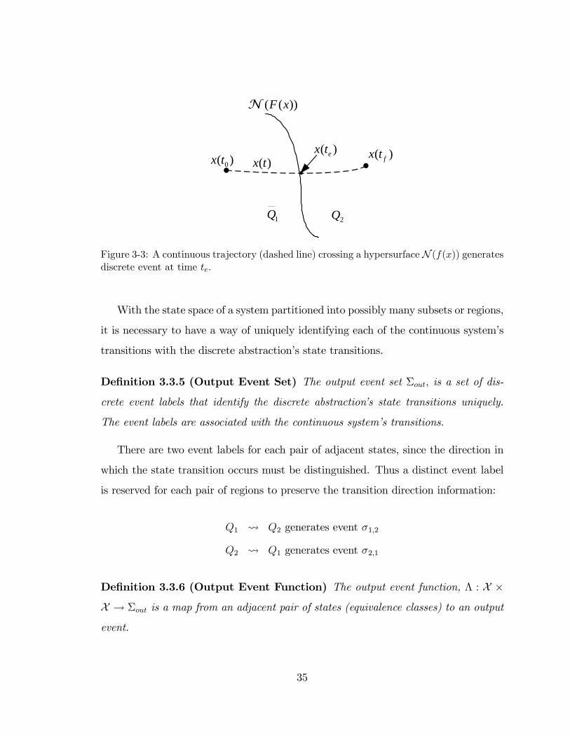
))(( xFN
1Q 2Q
)(tx)( 0tx )( ftx)( etx
Figure 3-3: A continuous trajectory (dashed line) crossing a hypersurfaceN (f(x)) generatesdiscrete event at time te.
With the state space of a system partitioned into possibly many subsets or regions,
it is necessary to have a way of uniquely identifying each of the continuous system�s
transitions with the discrete abstraction�s state transitions.
De�nition 3.3.5 (Output Event Set) The output event set �out; is a set of dis-
crete event labels that identify the discrete abstraction�s state transitions uniquely.
The event labels are associated with the continuous system�s transitions.
There are two event labels for each pair of adjacent states, since the direction in
which the state transition occurs must be distinguished. Thus a distinct event label
is reserved for each pair of regions to preserve the transition direction information:
Q1 Q2 generates event �1;2
Q2 Q1 generates event �2;1
De�nition 3.3.6 (Output Event Function) The output event function, � : X �
X ! �out is a map from an adjacent pair of states (equivalence classes) to an output
event.
35
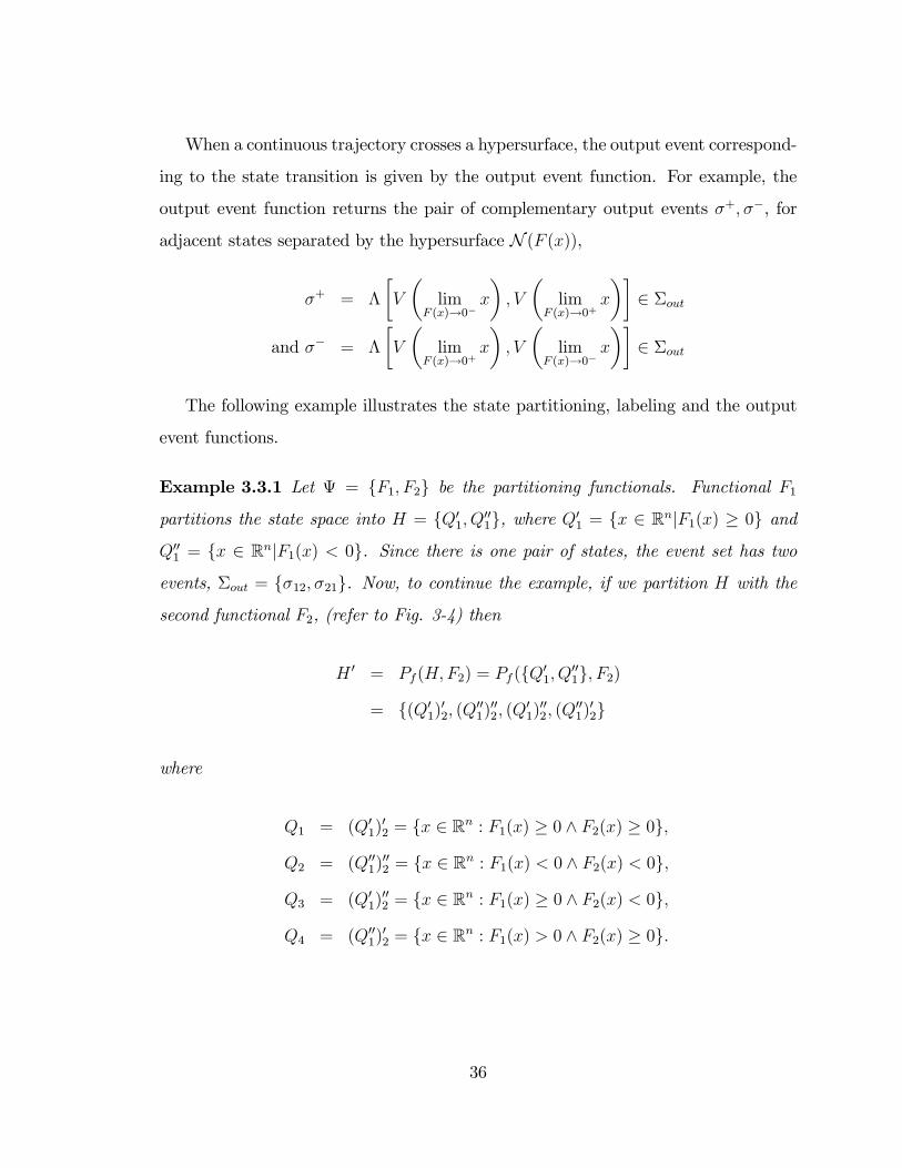
When a continuous trajectory crosses a hypersurface, the output event correspond-
ing to the state transition is given by the output event function. For example, the
output event function returns the pair of complementary output events �+; ��, for
adjacent states separated by the hypersurface N (F (x)),
�+ = �
�V
�lim
F (x)!0�x
�; V
�lim
F (x)!0+x
��2 �out
and �� = �
�V
�lim
F (x)!0+x
�; V
�lim
F (x)!0�x
��2 �out
The following example illustrates the state partitioning, labeling and the output
event functions.
Example 3.3.1 Let = fF1; F2g be the partitioning functionals. Functional F1
partitions the state space into H = fQ01; Q001g, where Q01 = fx 2 RnjF1(x) � 0g and
Q001 = fx 2 RnjF1(x) < 0g. Since there is one pair of states, the event set has two
events, �out = f�12; �21g. Now, to continue the example, if we partition H with the
second functional F2, (refer to Fig. 3-4) then
H 0 = Pf (H;F2) = Pf (fQ01; Q001g; F2)
= f(Q01)02; (Q001)002; (Q01)002; (Q001)02g
where
Q1 = (Q01)02 = fx 2 Rn : F1(x) � 0 ^ F2(x) � 0g;
Q2 = (Q001)002 = fx 2 Rn : F1(x) < 0 ^ F2(x) < 0g;
Q3 = (Q01)002 = fx 2 Rn : F1(x) � 0 ^ F2(x) < 0g;
Q4 = (Q001)02 = fx 2 Rn : F1(x) > 0 ^ F2(x) � 0g:
36
The discrete state labels are:
8x 2 Q1 V (x) =h1 1
iT8x 2 Q2; V (x) =
h0 0
iT8x 2 Q3; V (x) =
h1 0
iT8x 2 Q4; V (x) =
h0 1
iTEach of the states is adjacent to one another, so there are 6 pairs of sets in the state
space partition:
(Q1; Q2); (Q2; Q3); (Q3; Q4); (Q4; Q1); (Q1; Q3); (Q2; Q4)
therefore the cardinality of the output event set
j�outj =M !
(M � 2)! =4!
(4� 2)! =24
2= 12
and assigning labels to each transition gives the output event set is
�out = f�1;2; �2;1; �2;3; �3;2; �3;4; �4;3; �4;1; �1;4; �1;3; �3;1; �2;4; �4;2g
We will now develop the cardinality of the output event set given a family of
subsets.
Theorem 3.3.1 Let H = fQj � Rnj1 � j � Mg be a family of subsets. The
corresponding output event set �out has �nite cardinality and an upper bound of
j�outj = M !(M�2)! .
Proof. The upper bound occurs if every Qj is adjacent to every other Qj. This is
a permutation, since the order in which the open sets are paired matters. A pairwise
permutation forM objects is given by the formula for a so called r-permutation where
37
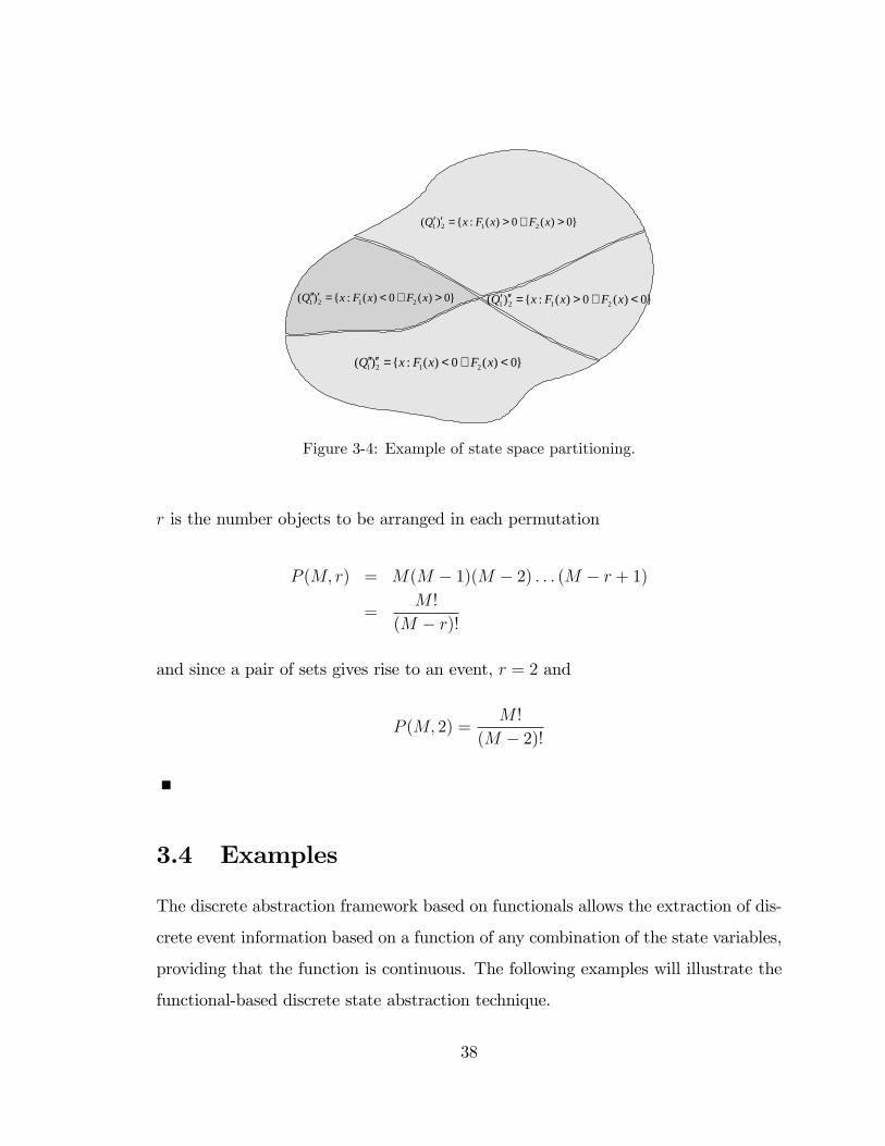
}0)(0)(:{)( 2121 >∧>=′′ xFxFxQ
}0)(0)(:{)( 2121 <∧<=′′′′ xFxFxQ
}0)(0)(:{)( 2121 <∧>=′′′ xFxFxQ}0)(0)(:{)( 2121 >∧<=′′′ xFxFxQ
Figure 3-4: Example of state space partitioning.
r is the number objects to be arranged in each permutation
P (M; r) = M(M � 1)(M � 2) : : : (M � r + 1)
=M !
(M � r)!
and since a pair of sets gives rise to an event, r = 2 and
P (M; 2) =M !
(M � 2)!
3.4 Examples
The discrete abstraction framework based on functionals allows the extraction of dis-
crete event information based on a function of any combination of the state variables,
providing that the function is continuous. The following examples will illustrate the
functional-based discrete state abstraction technique.
38
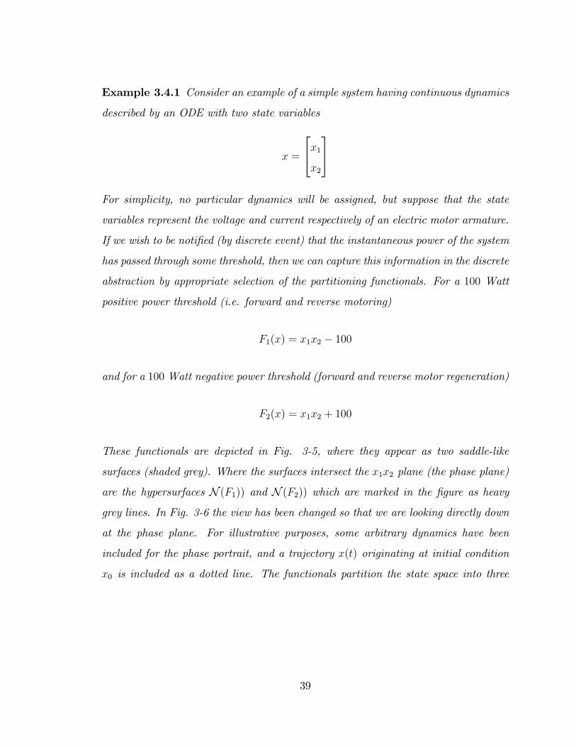
Example 3.4.1 Consider an example of a simple system having continuous dynamics
described by an ODE with two state variables
x =
24x1x2
35For simplicity, no particular dynamics will be assigned, but suppose that the state
variables represent the voltage and current respectively of an electric motor armature.
If we wish to be noti�ed (by discrete event) that the instantaneous power of the system
has passed through some threshold, then we can capture this information in the discrete
abstraction by appropriate selection of the partitioning functionals. For a 100 Watt
positive power threshold (i.e. forward and reverse motoring)
F1(x) = x1x2 � 100
and for a 100Watt negative power threshold (forward and reverse motor regeneration)
F2(x) = x1x2 + 100
These functionals are depicted in Fig. 3-5, where they appear as two saddle-like
surfaces (shaded grey). Where the surfaces intersect the x1x2 plane (the phase plane)
are the hypersurfaces N (F1)) and N (F2)) which are marked in the �gure as heavy
grey lines. In Fig. 3-6 the view has been changed so that we are looking directly down
at the phase plane. For illustrative purposes, some arbitrary dynamics have been
included for the phase portrait, and a trajectory x(t) originating at initial condition
x0 is included as a dotted line. The functionals partition the state space into three
39

Figure 3-5: Equal power surfaces for discrete event generation on power threshold.
40
Figure 3-6: View of the phase plane, with hypersurfaces N (F1));N (F2)), and an illustrativetrajectory x(t).
41
states,
Q1 = fx : F1(x) < 0 ^ F2(x) < 0g
Q2 = fx : F1(x) > 0 ^ F2(x) < 0g
Q3 = fx : F1(x) < 0 ^ F2(x) > 0g
Clearly, the set fx : F1(x) > 0^F2(x) > 0g = ;. This continuous trajectory generates
four discrete events from the following state transitions
Q1 Q2
Q2 Q1
Q1 Q3
Q3 Q1
The discrete event labels may be evaluated using the event labeling function
�1;2 = �(Q1; Q2)
�2;1 = �(Q2; Q1)
�1;3 = �(Q1; Q3)
�3;1 = �(Q3; Q1)
Example 3.4.2 A further example will illustrate the natural expressiveness of the
functional partitioning technique, using a simple nonlinear ODE model of pendulum
with damping. The dynamics are described by
mld2�
dt2+ bl
d�
dt+mg sin � = 0
where m is the mass of the pendulum bob and l its length, b is a friction term, g is
42
the acceleration due to gravity, and, � is the pendulum angle . The state vector shall
be de�ned as
x =
24x1x2
35 =24�_�
35and then the state equations are
_x1 = x2
_x2 = �glsin x1 �
b
mx2
The total energy for this system is de�ned as the sum of the kinetic energy K and
potential energy P , which we will de�ne in the rotational coordinate frame.
E = K + P
where kinetic energy is
K =1
2m(lx2)
2
and the potential energy is
P = �mgl(cosx1)
The total energy expression E represents an equal energy surface when plotted as a
function of the state variables. If we wish to partition the state space such that the
states represent energy levels, we use the following functional
F (x) =1
2m(lx2)
2 +mgl(1� cosx1)� 9:81
this gives a hypersurface that partitions the state space into two discrete states; system
energy greater than 9:81 J and system energy less than 9:81 J. The potential energy
term in the expression has been modi�ed to change datum (zero energy when the bob
is at the bottom).This functional is depicted in Fig. 3-7 as a shaded grey surface. A
43

Figure 3-7: A partitioning functional F (x) based on the total energy in the pendulum system.
44
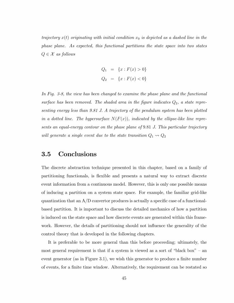
trajectory x(t) originating with initial condition x0 is depicted as a dashed line in the
phase plane. As expected, this functional partitions the state space into two states
Q 2 X as follows
Q1 = fx : F (x) > 0g
Q2 = fx : F (x) < 0g
In Fig. 3-8, the view has been changed to examine the phase plane and the functional
surface has been removed. The shaded area in the �gure indicates Q2, a state repre-
senting energy less than 9.81 J. A trajectory of the pendulum system has been plotted
in a dotted line. The hypersurface N(F (x)), indicated by the ellipse-like line repre-
sents an equal-energy contour on the phase plane of 9:81 J. This particular trajectory
will generate a single event due to the state transition Q1 Q2
3.5 Conclusions
The discrete abstraction technique presented in this chapter, based on a family of
partitioning functionals, is �exible and presents a natural way to extract discrete
event information from a continuous model. However, this is only one possible means
of inducing a partition on a system state space. For example, the familiar grid-like
quantization that an A/D convertor produces is actually a speci�c case of a functional-
based partition. It is important to discuss the detailed mechanics of how a partition
is induced on the state space and how discrete events are generated within this frame-
work. However, the details of partitioning should not in�uence the generality of the
control theory that is developed in the following chapters.
It is preferable to be more general than this before proceeding; ultimately, the
most general requirement is that if a system is viewed as a sort of �black box��an
event generator (as in Figure 3.1), we wish this generator to produce a �nite number
of events, for a �nite time window. Alternatively, the requirement can be restated so
45
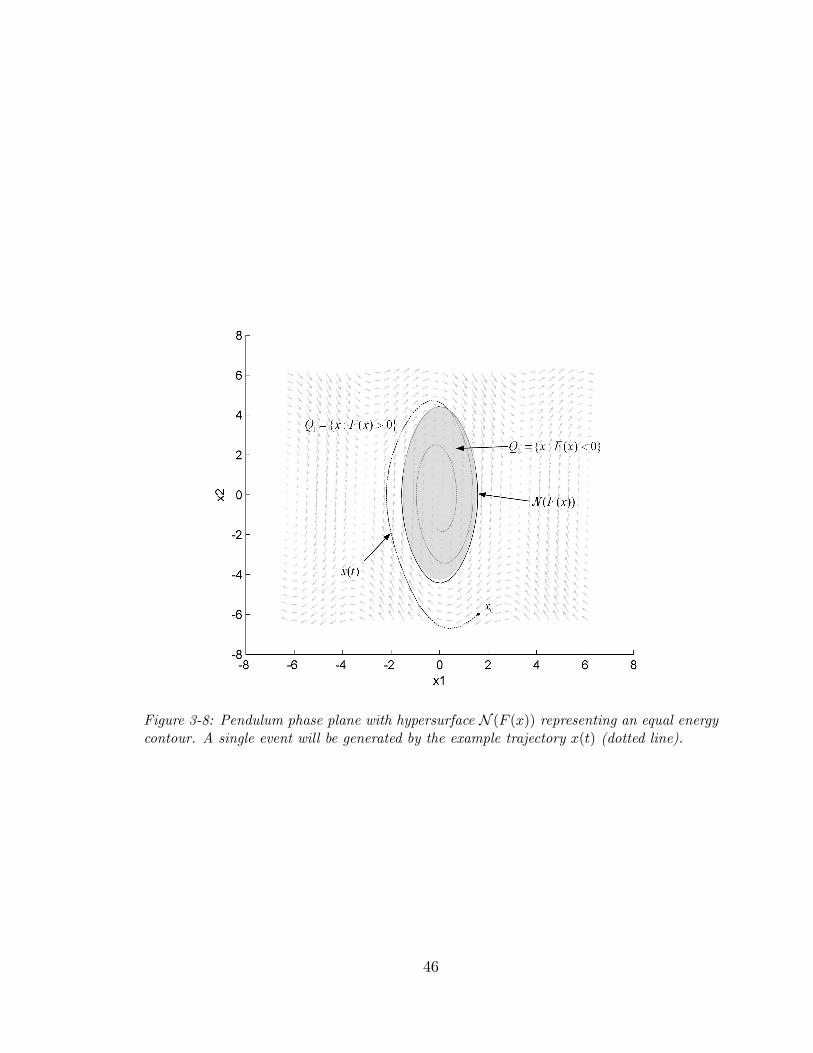
Figure 3-8: Pendulum phase plane with hypersurface N (F (x)) representing an equal energycontour. A single event will be generated by the example trajectory x(t) (dotted line).
46
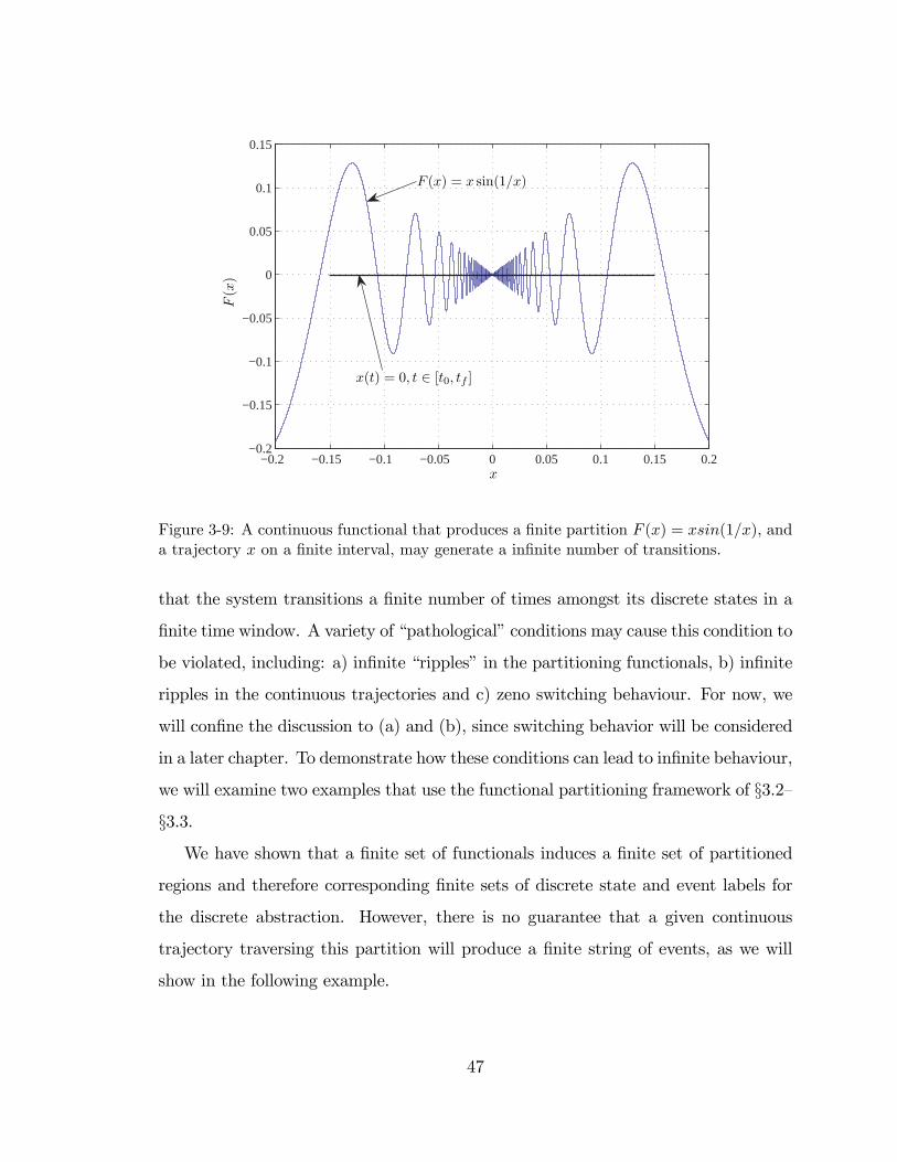
−0.2 −0.15 −0.1 −0.05 0 0.05 0.1 0.15 0.2−0.2
−0.15
−0.1
−0.05
0
0.05
0.1
0.15
x(t) = 0, t ∈ [t0, tf ]
F (x) = x sin(1/x)
F(x
)
x
Figure 3-9: A continuous functional that produces a �nite partition F (x) = xsin(1=x), anda trajectory x on a �nite interval, may generate a in�nite number of transitions.
that the system transitions a �nite number of times amongst its discrete states in a
�nite time window. A variety of �pathological�conditions may cause this condition to
be violated, including: a) in�nite �ripples�in the partitioning functionals, b) in�nite
ripples in the continuous trajectories and c) zeno switching behaviour. For now, we
will con�ne the discussion to (a) and (b), since switching behavior will be considered
in a later chapter. To demonstrate how these conditions can lead to in�nite behaviour,
we will examine two examples that use the functional partitioning framework of §3.2�
§3.3.
We have shown that a �nite set of functionals induces a �nite set of partitioned
regions and therefore corresponding �nite sets of discrete state and event labels for
the discrete abstraction. However, there is no guarantee that a given continuous
trajectory traversing this partition will produce a �nite string of events, as we will
show in the following example.
47

−0.16 −0.14 −0.12 −0.1 −0.08 −0.06 −0.04 −0.02 0−0.02
−0.015
−0.01
−0.005
0
0.005
0.01
x(t
)
t
t2 sin(1/t)
Figure 3-10: The trajectory x(t) = t2sin(1=t) on a �nite interval, produces an in�nitenumber of transitions.
Example 3.5.1 Consider a continuous dynamical system modeled by _x = f(x; t)
with system state space x 2 R and let F be a smooth continuous functional
F (x) =
8<: x sin( 1x) x 6= 0
0 x = 0
Then suppose there exists a continuous trajectory x which is a solution of f , for a
�nite time interval [t0; tf ] such that x(t) = 0; for all t 2 [t0; tf ] and the initial condition
x0 = x(t0) = �0:15 (Fig. 3-9). Although this partition induces a pair of regions, or
discrete states, on a �nite time interval this trajectory can clearly generate an in�nite
number of events.
Likewise, a similar example can be contrived to show that certain continuous
trajectories may also lead to in�nite events.
Example 3.5.2 Suppose the dynamics of a system are modeled by the Lipschitz-
48
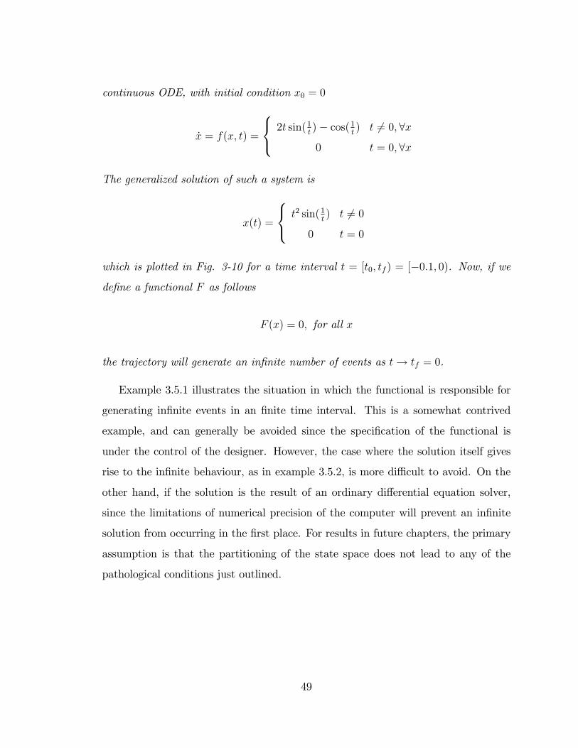
continuous ODE, with initial condition x0 = 0
_x = f(x; t) =
8<: 2t sin(1t)� cos(1
t) t 6= 0;8x
0 t = 0;8x
The generalized solution of such a system is
x(t) =
8<: t2 sin(1t) t 6= 0
0 t = 0
which is plotted in Fig. 3-10 for a time interval t = [t0; tf ) = [�0:1; 0). Now, if we
de�ne a functional F as follows
F (x) = 0; for all x
the trajectory will generate an in�nite number of events as t! tf = 0.
Example 3.5.1 illustrates the situation in which the functional is responsible for
generating in�nite events in an �nite time interval. This is a somewhat contrived
example, and can generally be avoided since the speci�cation of the functional is
under the control of the designer. However, the case where the solution itself gives
rise to the in�nite behaviour, as in example 3.5.2, is more di¢ cult to avoid. On the
other hand, if the solution is the result of an ordinary di¤erential equation solver,
since the limitations of numerical precision of the computer will prevent an in�nite
solution from occurring in the �rst place. For results in future chapters, the primary
assumption is that the partitioning of the state space does not lead to any of the
pathological conditions just outlined.
49
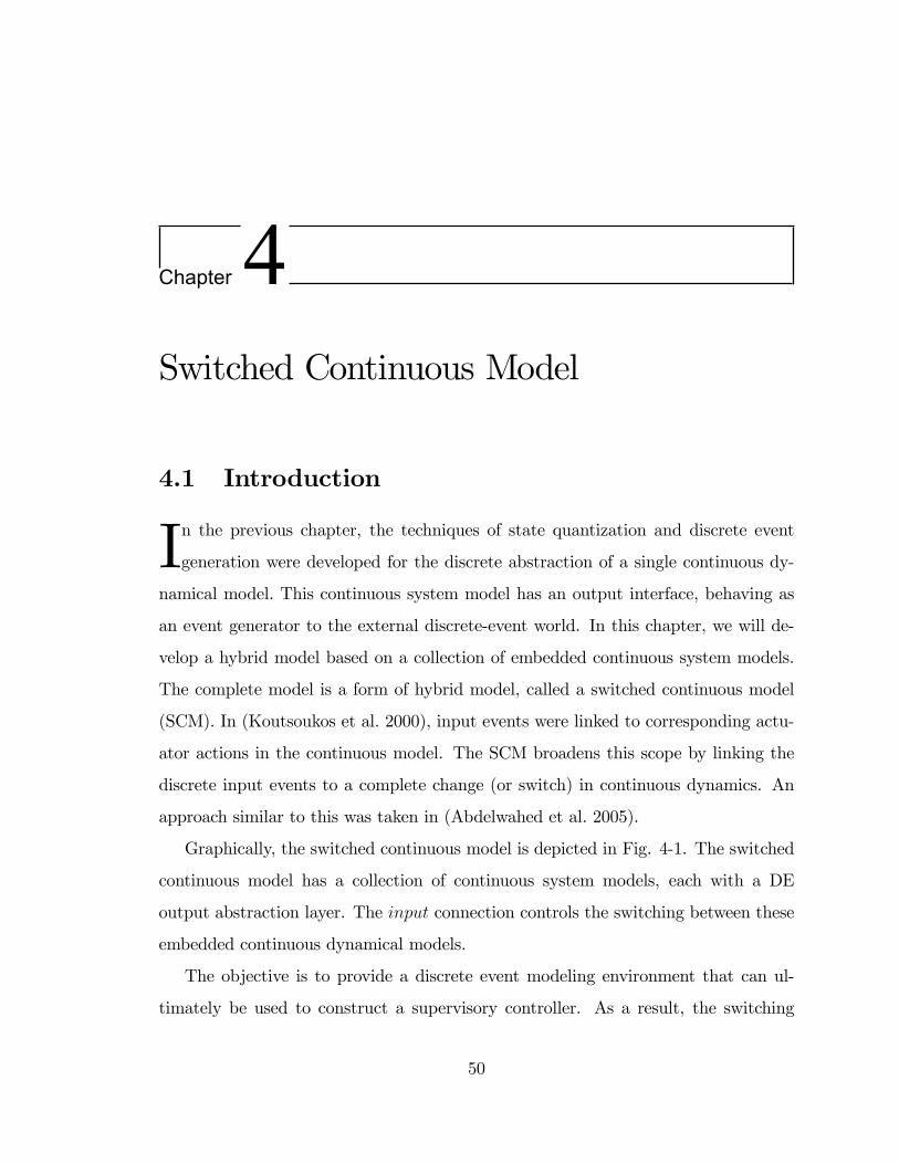
Chapter4Switched Continuous Model
4.1 Introduction
In the previous chapter, the techniques of state quantization and discrete eventgeneration were developed for the discrete abstraction of a single continuous dy-
namical model. This continuous system model has an output interface, behaving as
an event generator to the external discrete-event world. In this chapter, we will de-
velop a hybrid model based on a collection of embedded continuous system models.
The complete model is a form of hybrid model, called a switched continuous model
(SCM). In (Koutsoukos et al. 2000), input events were linked to corresponding actu-
ator actions in the continuous model. The SCM broadens this scope by linking the
discrete input events to a complete change (or switch) in continuous dynamics. An
approach similar to this was taken in (Abdelwahed et al. 2005).
Graphically, the switched continuous model is depicted in Fig. 4-1. The switched
continuous model has a collection of continuous system models, each with a DE
output abstraction layer. The input connection controls the switching between these
embedded continuous dynamical models.
The objective is to provide a discrete event modeling environment that can ul-
timately be used to construct a supervisory controller. As a result, the switching
50
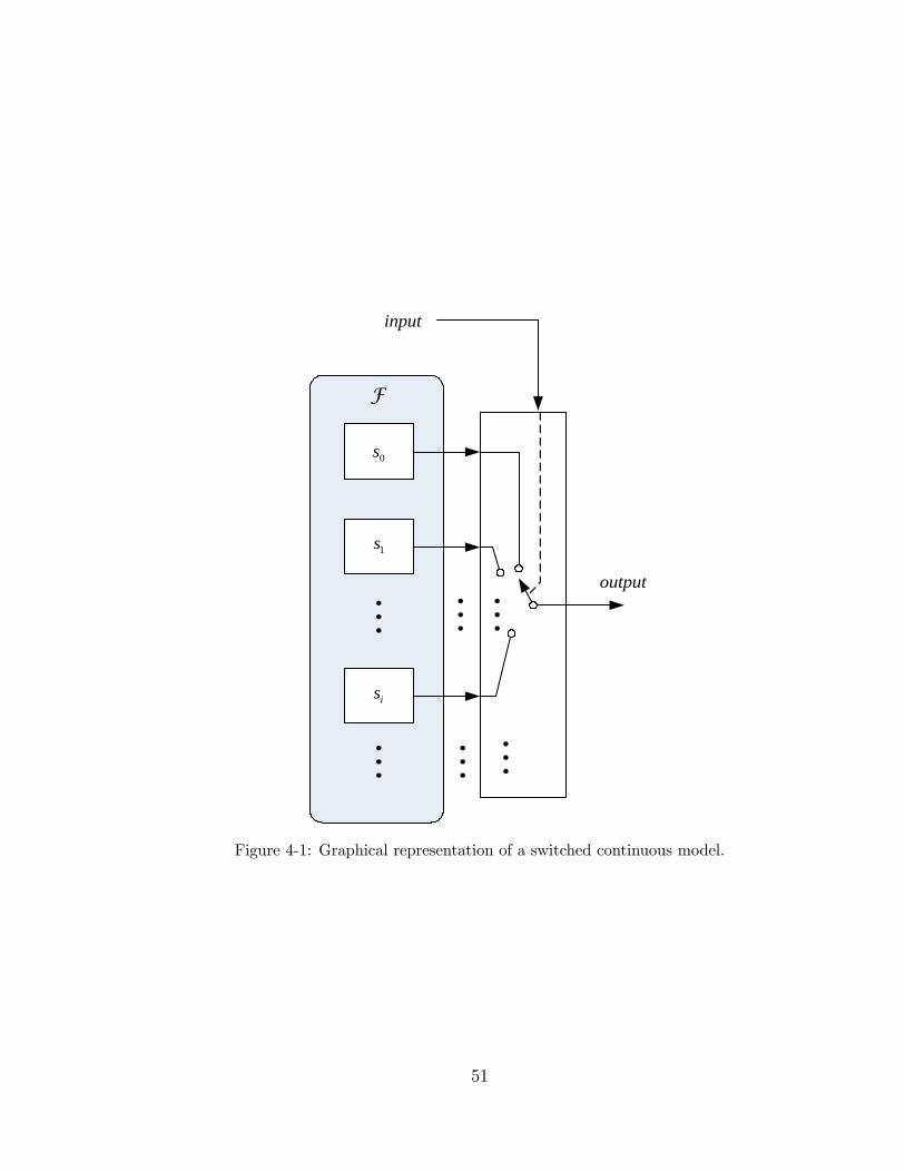
output
0s
F
1s
is
input
Figure 4-1: Graphical representation of a switched continuous model.
51
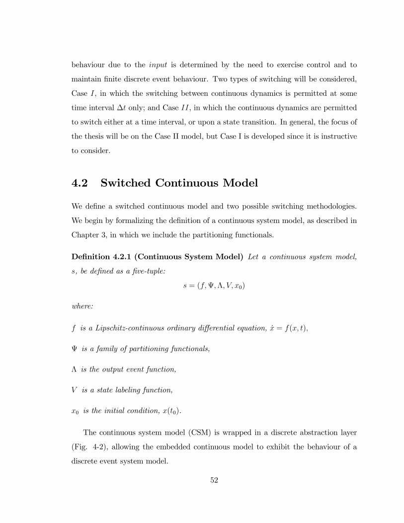
behaviour due to the input is determined by the need to exercise control and to
maintain �nite discrete event behaviour. Two types of switching will be considered,
Case I, in which the switching between continuous dynamics is permitted at some
time interval �t only; and Case II, in which the continuous dynamics are permitted
to switch either at a time interval, or upon a state transition. In general, the focus of
the thesis will be on the Case II model, but Case I is developed since it is instructive
to consider.
4.2 Switched Continuous Model
We de�ne a switched continuous model and two possible switching methodologies.
We begin by formalizing the de�nition of a continuous system model, as described in
Chapter 3, in which we include the partitioning functionals.
De�nition 4.2.1 (Continuous System Model) Let a continuous system model,
s, be de�ned as a �ve-tuple:
s = (f;;�; V; x0)
where:
f is a Lipschitz-continuous ordinary di¤erential equation, _x = f(x; t);
is a family of partitioning functionals,
� is the output event function,
V is a state labeling function,
x0 is the initial condition, x(t0).
The continuous system model (CSM) is wrapped in a discrete abstraction layer
(Fig. 4-2), allowing the embedded continuous model to exhibit the behaviour of a
discrete event system model.
52
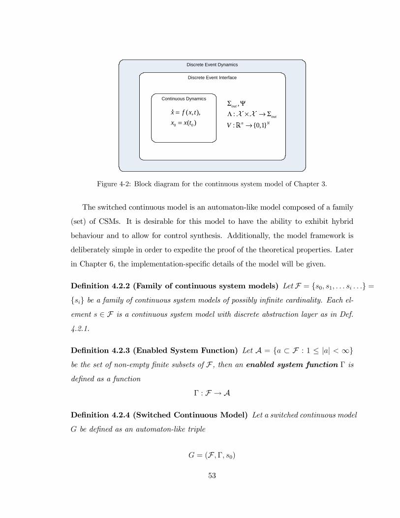
Discrete Event Dynamics
Discrete Event Interface
,
:
: {0,1}
out
out
n NV
Σ ΨΛ × → Σ
→
X X
R
Continuous Dynamics
0 0
( , ),
( )
x f x t
x x t
==
�
Figure 4-2: Block diagram for the continuous system model of Chapter 3.
The switched continuous model is an automaton-like model composed of a family
(set) of CSMs. It is desirable for this model to have the ability to exhibit hybrid
behaviour and to allow for control synthesis. Additionally, the model framework is
deliberately simple in order to expedite the proof of the theoretical properties. Later
in Chapter 6, the implementation-speci�c details of the model will be given.
De�nition 4.2.2 (Family of continuous system models) Let F = fs0; s1; : : : si : : :g =
fsig be a family of continuous system models of possibly in�nite cardinality. Each el-
ement s 2 F is a continuous system model with discrete abstraction layer as in Def.
4.2.1.
De�nition 4.2.3 (Enabled System Function) Let A = fa � F : 1 � jaj < 1g
be the set of non-empty �nite subsets of F , then an enabled system function � is
de�ned as a function
� : F ! A
De�nition 4.2.4 (Switched Continuous Model) Let a switched continuous model
G be de�ned as an automaton-like triple
G = (F ;�; s0)
53
where:
F is a family of continuous system models (Def. 4.2.2)
� is the enabled system function (Def. 4.2.3)
s0 is the initial continuous system model
The switched continuous model has behaviour similar to a multiplexor (Fig. 4-1).
The switch function permits only one continuous system model to be selected at any
instant in time.
De�nition 4.2.5 (Execution) An execution of a switched continuous model is de-
�ned as a sequence v, of selected continuous system models
v = fs0; s1; : : : s� : : :g
An execution of a system modeled by a SCM starts with the selection of the initial
continuous system model s0. At some point in time, the system will switch to, or
select, another continuous system model.
De�nition 4.2.6 (Choice Point) Let G = (F ;�; s0) be a SCM, and let s0 be the
currently selected CSM. The point in time at which the SCM switches execution to
another continuous system model s00 is known as a choice point. The switches occur
either due to a time event (tick, or t) or due to a state transition within the currently
selected CSM, s0.
A choice point can be thought of as the moment a controller exercises control. In
Case I switching, choice points occur at some time interval, not necessarily with a
constant time spacing. Case I switching is analogous to that of a PLC in industrial
practice, in which the controller polls it�s inputs and updates control outputs on some
time schedule.
54
The enabled system function �; of Def. 4.2.3, is an implementation-dependent
map. It returns a �nite set of continuous system models and is invoked at the choice
points. The function is a convenient method of de�ning the future execution of the
SCM recursively, and is an abstraction of the actual control algorithm. Since the
switched continuous model is an abstraction of a real system, there must always be
a system eligible for execution, hence the requirement that the set of enabled system
models be non-empty j�(s)j � 1.
De�nition 4.2.7 (Successor Continuous System Model) Let s 2 F be a con-
tinuous system model, then any element of the family, s0 2 �(s) at some choice point
is a successor CSM of s.
De�nition 4.2.8 (Control) Let the currently selected model be s 2 F . The selec-
tion of a single successor continuous system model s0 from the set of eligible successor
CSMs �(s); referred to as control of the modeled system.
In Fig. 4-1 the SCM is illustrated as a multiplexor with a switching (or control)
input. We will associate the selection of continuous systemmodels by a controller with
discrete (input) events. At each choice point, the controller may select a continuous
system model to execute. To ensure the �niteness of the switching behaviour in the
SCM, the control choice must always be �nite. Recall from Def. 4.2.3, � : F ! A,
where A = f� � F : 1 � j�j < 1g represents the �nite set of enabled continuous
systemmodel for a particular choice point. The SCM input control interface associates
each element s 2 �, with a unique input event label.
De�nition 4.2.9 (Input Event Set) Let G = (F ;�; s0) be an SCM. Then let �inbe a set of input event labels such that there exists a unique input event label �i 2 �infor every enabled continuous system model at each choice point 8si 2 �(s).
The historical (past) execution of a CSM is clearly a simple sequence. However,
due to the fact that j�(s)j at a choice point may be greater than one, then there are
55
a number of possible future executions of the SCM, and a branch in the future (or
predicted) execution occurs.
Example 4.2.1 In Fig. 4-3, a future execution tree (prediction) is illustrated. Note
that the CSM subscripts for the diagram do not necessarily indicate any sort of sequen-
tial order, they are simply distinguishing labels. Beginning with the initial CSM s0,
a choice point occurs, indicated on the time axis as a tick (of the universal timebase,
t). Evaluation of the enabled system function at the conclusion of the s0,
�(s0) = fs1; s2; s3g � F
then, projecting forward in time, each of the systems represents a branch in the future
execution of the SCM. Again, following the top branch, s1, at the next system choice
point we get,
�(s1) = fs4; s5; s6g � F
To summarize, � reduces the in�nite possible continuous system models F , to
a �nite subset of continuous models which are eligible for execution at each choice
point. Therefore, a prediction of the future CSM selection, is a branching tree. When
the SCM is executed, only a single CSM s0 2 �(s) � A is selected at any choice point,
and the execution of the model is a sequence of continuous system models.
4.3 Prediction - Case I Switching
We will now examine the future execution of the SCM. It is desirable to establish a
bound on the number of systems in the future execution; that is, the total reachable
systems under the time switching regime (Case I). To facilitate this, we begin by
de�ning an n-ary version of the enabled system function.
56
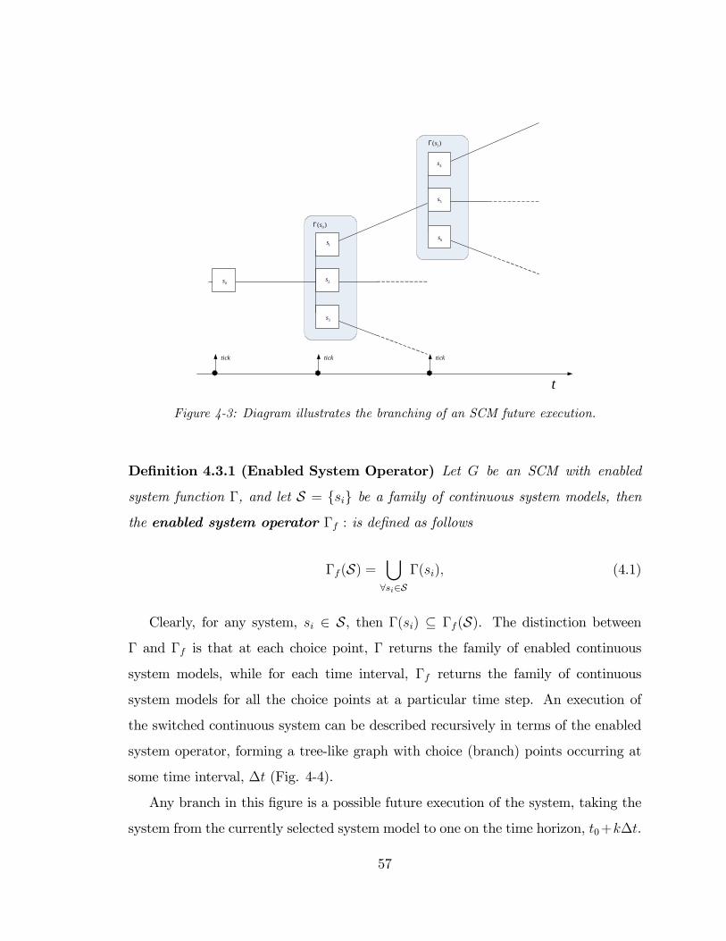
1s
2s
3s
0s
5s
6s
4s
tick tick tick
t
0( )sΓ
1( )sΓ
Figure 4-3: Diagram illustrates the branching of an SCM future execution.
De�nition 4.3.1 (Enabled System Operator) Let G be an SCM with enabled
system function �, and let S = fsig be a family of continuous system models, then
the enabled system operator �f : is de�ned as follows
�f (S) =[8si2S
�(si); (4.1)
Clearly, for any system, si 2 S, then �(si) � �f (S). The distinction between
� and �f is that at each choice point, � returns the family of enabled continuous
system models, while for each time interval, �f returns the family of continuous
system models for all the choice points at a particular time step. An execution of
the switched continuous system can be described recursively in terms of the enabled
system operator, forming a tree-like graph with choice (branch) points occurring at
some time interval, �t (Fig. 4-4).
Any branch in this �gure is a possible future execution of the system, taking the
system from the currently selected system model to one on the time horizon, t0+k�t.
57
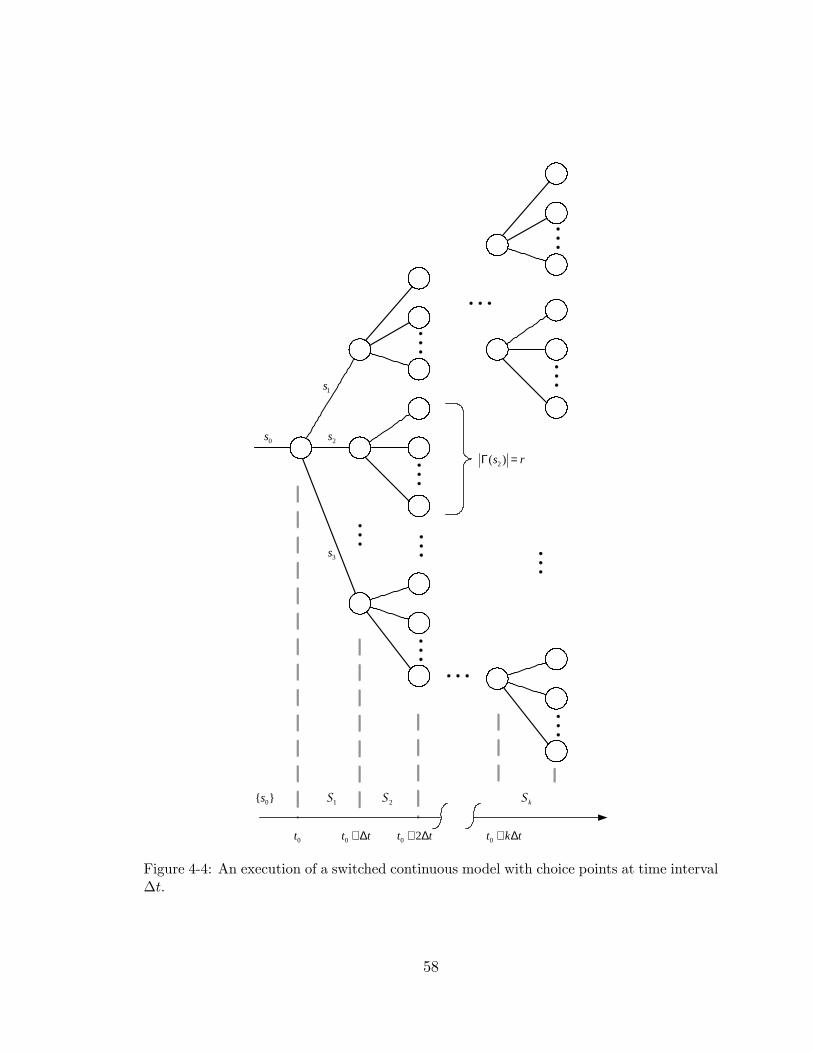
kS2S1S0{ }s
2( )s rΓ =
0s
1s
2s
3s
0t 0t t+ ∆ 0 2t t+ ∆ 0t k t+ ∆
Figure 4-4: An execution of a switched continuous model with choice points at time interval�t.
58
De�nition 4.3.2 (Families of Continuous System Models) Let G = (F ;�; s0)
be a switched continuous model and let p be the number of time intervals, �t, over
which the model will be executed. Let Sk be the kth family of continuous system
models, at integer k � 1 time steps from the selection of the initial system, s0. This
family can be expressed in terms of recursive enabled system operations:
Sk = �f (: : :�f (| {z }k times
fs0g) : : :) (4.2)
Time is implicit in this equation and in Fig. 4-4, with each nested �f operator being
evaluated at a choice point. Each choice point occurs due to the passage of an interval
of time, �t.
We now show that the number of eligible continuous system models for future
execution may grow exponentially with time. The following proof establishes the size
of �f at any time step.
Lemma 4.3.1 For a switched continuous model, the cardinality of the family of en-
abled continuous system models at the kth time step for integer k � 1, as per Eq. 4.2,
has upper bound of jSkj = rk, provided that at each choice point there are at most r
possible continuous system models to switch amongst.
Proof. The lemma can be proven by assuming maximal switching, and using
induction on k. For the base case, k = 1, the cardinality of the �rst family of enabled
continuous system models, jS1j � j�(fs0g)j = r, which is consistent with rk since
r1 = r. The inductive hypothesis is that jSkj � rk. The family of continuous system
models enabled at k switches from the initial system, s0 is Sk and the cardinality is
59
jSkj � rk. By Eq. 4.2 then:
jSk+1j = j�f (Sk)j
=
����� S8si2Sk �(si)�����
= j�(s1)j+ j�(s2)j+ : : :+ j�(srk)j
� r + r + : : :+ r| {z }rk times
= rk � r
jSk+1j � rk+1
thus proving the inductive hypothesis to be correct.
De�nition 4.3.3 (Reachable CSM) Let (F ;�; s0) be a SCM. A continuous system
model s0 2 F is said to be reachable from s0 if there is a future execution v such that
s0 2 v
v = fs0; : : : ; s0; : : :g
Now we wish to get an expression for the size of the set of reachable continuous
system models SR for some arbitrary number of time steps.
De�nition 4.3.4 (Reachable Set of Continuous System Models) Let G = (F ;�; s0)
be a switched continuous model, then the family of continuous system models that is
reachable from s0 (including s0 itself) in p time steps, SR, is de�ned recursively as
the union for k = 1; 2; : : : ; p, of each of the families in Eq. 4.2 , as follows:
SR = fs0g[0@ p[
k=1
�f (: : :�f (| {z }k times
fs0g) : : :)
1A (4.3)
Lemma 4.3.2 Let G = (F ;�; s0) be a switched continuous model executed on a �nite
number of time intervals, p � 1. Let the cardinality of the family of enabled continuous
system models at any choice point be j�(si)j � r for all si 2 F , then the family of
60
continuous system models, SR, reachable from the initial continuous system model,
s0, as de�ned in Eq. 4.3, has the following cardinality:
jSRj �rp+1 � 1r � 1 (4.4)
Proof. By Lemma 4.3.1, the cardinality of the kth family of enabled continuous
system models is given by jSkj = rk. And the reachable set of continuous system
models is, by Eq. 4.3,
jSRj =
������fs0g[24 p[
k=1
�f (: : :�f (| {z }k
fs0g) : : :)
35������= 1 + jS1j+ jS2j+ : : :+ jSpj
� r0 + r1 + r2 + :::rp
the sum of this geometric series is
pXk=0
rk =
8<: rp+1�1r�1 r 6= 1
p+ 1 r = 1
Thus we have proven a general closed form expression for the upper bound for the
cardinality of the reachable continuous system models. Since the number of possible
enabled systems at any choice point is unpredictable, it is possible only to establish an
expression for the upper bound on the cardinality of the set of reachable continuous
system models.
De�nition 4.3.5 Let maximal switching be de�ned as: for all choice points, there
are exactly j�(si)j = r continuous system models to switch between.
De�nition 4.3.6 Let minimal switching be de�ned as for all choice points, there
is one choice of continuous system model to switch to, j�(si)j = 1, for all si 2 SR.
61
Theorem 4.3.1 (Continuous System Reachability) Let Gc = (F ;�; s0) be a
switched continuous model. For a switching time interval of �t, a �nite number
of time intervals, p > 0, and the maximum enabled systems at any choice point �-
nite 1 � j�(si)j � r, for all si 2 F , then the family of continuous system models,
SR, reachable from the initial continuous system model, s0, as de�ned in Eq. 4.2, is
�nite, and furthermore,
p+ 1 � jSRj �rp+1 � 1r � 1
Proof. The reachable family of continuous system models is bounded above by
maximal switching, j�(si)j = r, for all si 2 SR: By Lemma 4.3.2, if both p and r are
�nite, the cardinality of summation of Eq. 4.4, jSRj, must also be �nite. The lower
bound is for the condition of minimal switching,
jSRj = 1 + jS1j+ jS2j+ : : :+ jSpj
= 1 + 1 + : : :+ 1| {z }p
= p+ 1
4.4 Prediction - Case II Switching
In §4.2, the switched continuous model was constrained to switch between models on
some time interval, �t. It will now be extended to permit switching of continuous
dynamics when a continuous trajectory transitions a partition boundary. This implies
that additional choice points (branching points) may occur between time intervals.
The goal is to show that the �nite properties of this model are maintained under
partition switching conditions, and to establish an upper bound on the cardinality of
the reachable state space.
For purposes of controlling the model, it was stated earlier that time switching
62
(Case I) was analogous to the update cycle of an industrial PLC, occurring at some
regular (or possibly multirate) scan time. Partition switching can be viewed as giv-
ing the controller the opportunity to react to an unscheduled alarm, similar to an
interrupt-driven control action of a real-time control task. Thus the Case II SCM
switching framework models the control of hybrid plants when a controller is permit-
ted to perform both synchronous and asynchronous control actions on the plant.
De�nition 4.4.1 (Partition Switching) A choice point occurs due to a state tran-
sition occurring within the currently selected continuous system model.
As was stated earlier, any complete branch from left to right in Fig. 4-5, is a
possible future execution v of the SC system model.
De�nition 4.4.2 (Execution Cardinality) The cardinality of a �nite execution v
is the number of elements (continuous system models) in the sequence, and is indicated
with the notation of set cardinality jvj.
First we will determine the cardinality of the reachable set of continuous models
for a single time interval �t, then extend it to multiple time intervals.
Lemma 4.4.1 Let G = (F ;�; s0) be a switched continuous model with partition
switching, and an upper bound on branching at each choice point, j�(si)j � r. Let
S�t be the reachable continuous system models in one time interval �t. Let vm be an
execution with the most partition switches in time interval, �t, such that jvmj = q.
If every execution v has �nite cardinality 0 � jvj � q, then the family of reachable
continuous system models from s0 in one �t is of �nite cardinality:
1 � jS�tj �rq+1 � 1r � 1 (4.5)
Proof. The proof is identical to that of Lemma 4.3.2. The family of enabled
continuous system models at k switches from s0 is denoted as Sk, and its cardinality
63
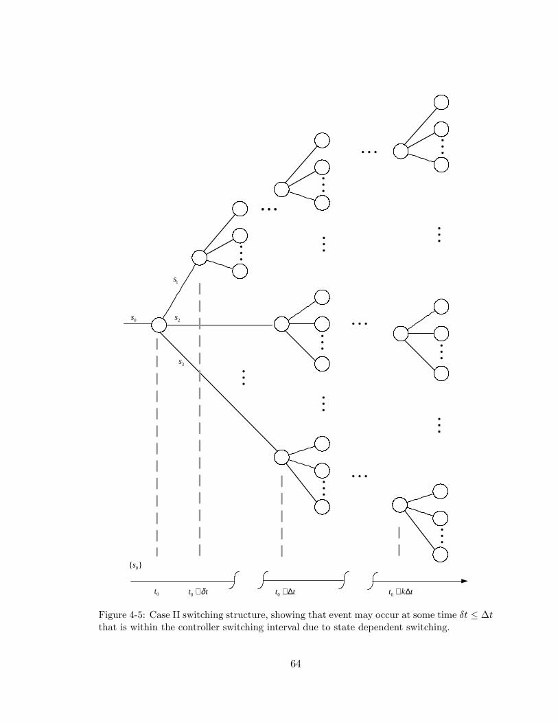
0{ }s
0s
1s
2s
3s
0t 0t tδ+ 0t t+ ∆ 0t k t+ ∆
Figure 4-5: Case II switching structure, showing that event may occur at some time �t � �tthat is within the controller switching interval due to state dependent switching.
64
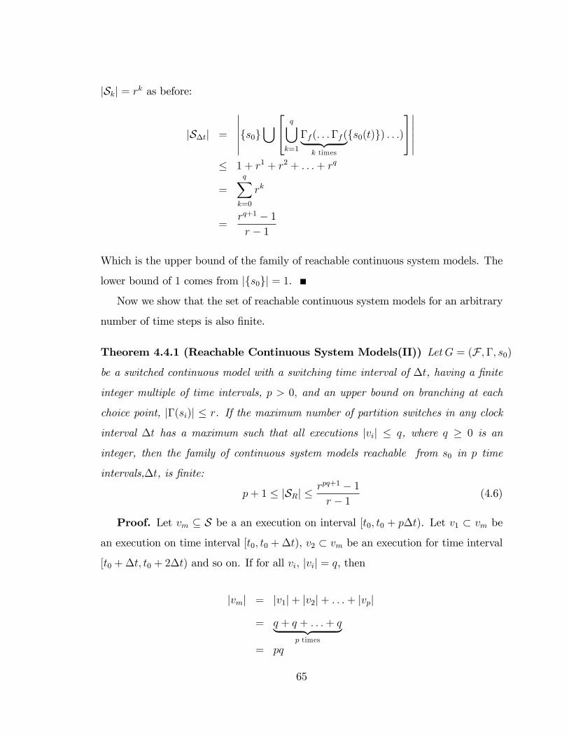
jSkj = rk as before:
jS�tj =
������fs0g[24 q[
k=1
�f (: : :�f (| {z }k times
fs0(t)g) : : :)
35������� 1 + r1 + r2 + : : :+ rq
=
qXk=0
rk
=rq+1 � 1r � 1
Which is the upper bound of the family of reachable continuous system models. The
lower bound of 1 comes from jfs0gj = 1.
Now we show that the set of reachable continuous system models for an arbitrary
number of time steps is also �nite.
Theorem 4.4.1 (Reachable Continuous System Models(II)) Let G = (F ;�; s0)
be a switched continuous model with a switching time interval of �t, having a �nite
integer multiple of time intervals, p > 0; and an upper bound on branching at each
choice point, j�(si)j � r. If the maximum number of partition switches in any clock
interval �t has a maximum such that all executions jvij � q, where q � 0 is an
integer, then the family of continuous system models reachable from s0 in p time
intervals,�t, is �nite:
p+ 1 � jSRj �rpq+1 � 1r � 1 (4.6)
Proof. Let vm � S be a an execution on interval [t0; t0 + p�t). Let v1 � vm be
an execution on time interval [t0; t0 +�t), v2 � vm be an execution for time interval
[t0 +�t; t0 + 2�t) and so on. If for all vi, jvij = q, then
jvmj = jv1j+ jv2j+ : : :+ jvpj
= q + q + : : :+ q| {z }p times
= pq
65

The largest reachable set occurs if every switched continuous trajectory produces pq
switches with maximal switching, j�(�)j = r, at each of the corresponding choice
points. The proof follows directly from Lemma 4.3.2:
jSRj =
������fs0g[24 pq[
k=1
�f (: : :�f (| {z }k
fs0g) : : :)
35������� 1 + r1 + r2 + : : :+ rpq
=
pqXk=0
rk
=rpq+1 � 1r � 1 ; for r > 0
and the lower bound is for minimal switching, r = j�(�)j = 1; and no partition switches
within each time interval, q = 0 for all choice points. The lower bound reduces to
that of Case I as in theorem 4.3.1:
jSRj = 1 + jS1j+ jS2j+ : : :+ jSpj
� 1 + 1 + 1 + : : :+ 1| {z }p times
= p+ 1
So, for a maximum �nite number of partition switches within one time interval q,
a maximum �nite number of eligible CSMs at each switch r; and a �nite number of
time intervals p, the reachable set of continuous system models is also �nite.
4.5 Continuous Dynamics
Up to this point, we have deliberately ignored the discrete and continuous dynamics
of the SCM, as we have dealt with the qualities of execution and reachability of the
continuous system models within the two switching frameworks. The details of the
66
underlying CSMs (time, continuous dynamics and discrete event dynamics) and their
contribution to the switching was hinted at in the de�nition of choice points. We now
examine the reachability properties of the continuous state space of the SCM, in the
context of the switching frameworks.
De�nition 4.5.1 (Solution of Continuous System Model) Let si = (f;; x0)
be a continuous system model for the time interval [t0; tf ) then the solution to the
IVP thus posed is
xi(t) = x0 +
tfZt0
f(x; �)d� , for t 2 [t0; tf )
exists and is unique.
So for the period of time while a continuous state model is selected, there is a
continuous state vector that is uniquely determined by the CSM�s initial condition and
dynamics. Since an execution v of the SCM consists of a sequence of selected CSMs,
then the continuous state of the SCM is easily de�ned in terms of the corresponding
sequence of solutions (or continuous trajectories).
Notation 4.5.1 Care should be taken to distinguish a point in a solution from a
solution on an interval. In general, a point of a solution will be denoted as a solution
evaluated at a point in time
x(ta) 2 Rn is the point of a solution evaluated at time ta
For a solution, xa(t) the reference to time will be omitted to reduce notational com-
plexity
xa is a solution as a function of time, a is an index
An exception to these notation conventions is the initial condition of a continuous
system model, x0 2 Rn which is a point. If there is likely to be confusion, the solution
will be referred to as a function of time, while a point is a solution explicitly evaluated
67
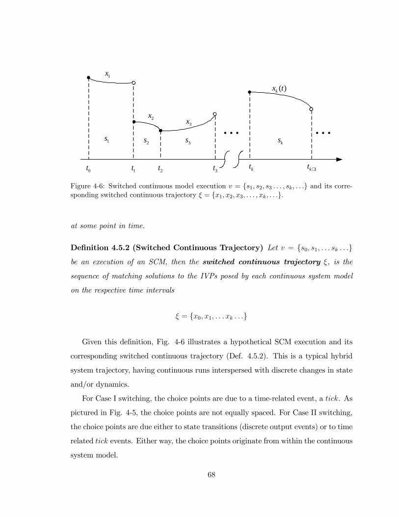
1s 2s 3s ks
1x
0t 1t 2t 3t kt 1kt +
2x3x
( )kx t
Figure 4-6: Switched continuous model execution v = fs1; s2; s3 : : : ; sk; : : :g and its corre-sponding switched continuous trajectory � = fx1; x2; x3; : : : ; xk; : : :g.
at some point in time.
De�nition 4.5.2 (Switched Continuous Trajectory) Let v = fs0; s1; : : : sk : : :g
be an execution of an SCM, then the switched continuous trajectory �, is the
sequence of matching solutions to the IVPs posed by each continuous system model
on the respective time intervals
� = fx0; x1; : : : xk : : :g
Given this de�nition, Fig. 4-6 illustrates a hypothetical SCM execution and its
corresponding switched continuous trajectory (Def. 4.5.2). This is a typical hybrid
system trajectory, having continuous runs interspersed with discrete changes in state
and/or dynamics.
For Case I switching, the choice points are due to a time-related event, a tick. As
pictured in Fig. 4-5, the choice points are not equally spaced. For Case II switching,
the choice points are due either to state transitions (discrete output events) or to time
related tick events. Either way, the choice points originate from within the continuous
system model.
68
Similarly to the de�nition for a successor CSM, we may de�ne a successor contin-
uous trajectory.
De�nition 4.5.3 (Successor Trajectory) Let sb be a successor continuous system
model of sa. Let xa be the solution to the IVP posed by sa on the time interval [t0; t1).
Then xb is the solution to the IVP posed by sb 2 �(sa) on the time interval [t1; t2).,
where t0 < t1 < t2, and xb is a successor continuous trajectory (or, alternately, the
successor solution) of xa. Notationally, we can say
xb = succ(xa)
De�nition 4.5.4 (Predecessor Trajectory) If xb is a successor continuous tra-
jectory of xa, then xa is the predecessor continuous trajectory of xb.
xa = pre(xb)
The successor function can be used to form an alternative de�nition of the switched
continuous trajectory using recursion.
De�nition 4.5.5 (Switched Continuous Trajectory) A switched continuous tra-
jectory �, is a set of continuous trajectories:
� = fxi : xi+1 = succ(xi)g, i = 1; 2; :::
The de�nition of a successor trajectory (Def. 4.5.3) ensures that any switched
continuous trajectory � has no "gaps" in time, nor does it have any "overlaps" in
time.
69
4.6 Continuous State Reachability
In §4.3 and §4.4, we examined the reachable continuous system models, and in the
previous section (§4.5), the relationship between a continuous system model and its
corresponding continuous state space was detailed. The reachable continuous state
space of the SCM can be de�ned in terms of switched continuous trajectories.
4.6.1 Case I Switching
Given a �nite prediction horizon in time, it is desirable to �nd an expression for
the reachable continuous state space. Let G = (F ;�; s0) be a SCM and let the state
prediction be de�ned for the time interval T = [t0; tf ) , where t0 is the initial execution
(or simulation) time and tf be the time horizon relative to t0.
De�nition 4.6.1 (Complete Switched Continuous Trajectory) A switched con-
tinuous trajectory, � = fx1; x2; : : : ; x�g is said to be complete on some time interval
(t0; tf ) if x1 is a solution to an IVP over a time interval starting at time t > t0, and
x� is a solution to an IVP over a time interval ending at tf .
A single complete SCT, �, on some interval of time is a depth-�rst reach, and
represents the reachable continuous state space corresponding to an execution v of
the SCM, G.
De�nition 4.6.2 (Reachable Continuous Solutions) Let G be a switched con-
tinuous model, then the state space reachable from x0 (the initial condition speci�ed
by CSM s0) on some time interval, T = [t0; tf ) is de�ned as:
R =[8�i
�i; �i are complete with respect to T
This de�nition indicates that the union of all complete switched continuous tra-
jectories for some time interval is the reachable state space. Computationally, the
70
reachable state space can be assembled by the union of all depth-�rst reaches.
Alternatively, the reachable state space can be de�ned in terms of the reachable
continuous system models.
De�nition 4.6.3 (Reachable State Space) Let Sk be the family of continuous
system models reachable from s0 in k time steps, as in Eq. 4.2. Let the time horizon
be a �nite number, p, of time steps, �t. The reachable state space of a switched con-
tinuous model is de�ned as the set of all solutions to the IVP�s posed by the reachable
sets of continuous system models
R = fx j 9k : 1 � k � p; 9s 2 Sk; x is a solution to sg
Lemma 4.6.1 (Finite Reachable State Space (I)) The cardinality of the con-
tinuous solutions in the reachable state space R is �nite:
p+ 1 � jRj�1� rp+1
1� r (4.7)
Proof. Due to Def. 4.5.1, there exists a direct correspondence between elements
the reach set R, and the reachable state space such that for all s 2 SR there exists
a unique solution x 2 R, by the earlier assumption of Lipschitz continuity of contin-
uous dynamics. Therefore, the cardinality result of Theorem 4.3.1 also holds for the
reachable state space R.
4.6.2 Case II Switching
We will establish the cardinality bounds for the reachable state space for Case II
switching. An important issue with a partition-switched model is the potential for
zeno execution. Models that have instantaneous switching of dynamics have the po-
tential for zeno execution. Zeno execution is technically an artifact of modeling, since
no real system can be zeno (Zhang, Johansson, Lygeros and Sastry 2000). However, it
71
is an undesirable condition in a model or simulation since it leads to in�nite switching
in a �nite period of time. In the case of the switched continuous model, only Case II
is prone to exhibit zeno executions.
De�nition 4.6.4 (Non-Zeno Switched Continuous Trajectory) A switched con-
tinuous trajectory, � on some �nite time interval, �t = [t0; tf ), is nonzeno if j�j � 1.
Assumption of nonzeno characteristics is problematic, since it may be di¢ cult
to predict in advance that a model will exhibit zeno executions (Heymann, Lin,
Meyer and Resmerita 2002). The assumption is that for Case II switching, all exe-
cutions are nonzeno. We base this assumption on the premise that zeno execution
can be avoided through the use of modi�ed models, or implementation-speci�c mod-
eling techniques, including temporal or spatial regularization (Johansson, Egerstedt,
Lygeros and Sastry 1999) or other zeno solution extension techniques. Indeed, in
Theorem 4.4.1, which claimed �niteness of the reachable set of continuous system
models, there was an implicit assumption of nonzeno execution1.
Lemma 4.6.2 (Finite Reachable State Space (II)) The cardinality of the con-
tinuous solutions in the reachable state space R is �nite and bounded above:
jRj � rpq+1 � 1r � 1 ; r > 1 (4.8)
Proof. For every continuous system model, si 2 SR there is a corresponding
solution to the IVP, xi 2 R, the cardinality of the reachable state space is identical
to Eq. 4.6, the cardinality of the reachable continuous system models for Case II
switching.
1Later, nonzenoness will be a necessary condition for existence of a controller (since the controlleris model-based).
72
4.7 Discrete Event Dynamics
The previous sections have examined the reachable continuous properties of the SCM.
This section will examine the discrete event properties of the SCM. Recall from §3.5
that a CSM under certain special conditions may generate in�nitely many transitions
on its partitioned state space within a �nite time interval. For the results of this
section, we must assume that the contrary condition is true, that is, no continuous
trajectory on a �nite time interval will generate in�nite transitions. This assumption
is justi�ed by the fact that no real system can behave in this way either by design, or
due to practical limitations such as �nite precision of calculations and �nite machine
cycle times.
4.7.1 Case I Switching
Proposition 4.7.1 (Finite Events (I)) Let G = (F ;�; s0) be a switched continu-
ous model, with switching time interval of �t, a �nite number of system switches,
p > 0, and an upper bound on switching at each choice point exists, j�(si)j � r, for
all si 2 F . If for all xi 2 R, the number of transitions generated ni for each solution
is �nite, then the reachable state space R will generate a �nite number of events due
to discrete state transitions.
Proof. Lemma 4.6.1 established that the cardinality of R is �nite, with upper
boundrp+1 � 1r � 1
Let ni denote the number of transitions generated by trajectory xi 2 R: The total
number of transitions, Ne, generated by G in p time steps is
Ne =
rp+1�1r�1Xi=1
ni
73

Since the limit of this sum is �nite and all ni are �nite, then Neis �nite.
4.7.2 Case II Switching
Proposition 4.7.2 (Finite Events (II)) Let G = (F ;�; s0) be a switched contin-
uous model, with a switching time interval of �t (clock), a �nite number of time
switches, p > 0. If an upper bound on switching at each choice point exists, j�(si)j �
r, for all si 2 F , if all switched continuous trajectories, �i, are nonzeno, and the max-
imum number of partition switches in any clock interval �t has a maximum, j�ij � q,
the reachable state space, R, will generate a �nite number of events due to discrete
state transitions (i.e. crossing partition boundaries).
Proof. By Lemma 4.6.2, the cardinality of the reachable state space is �nite,
with upper and lower bounds as indicated by Eq. 4.8. Since an event occurs at every
partition crossing, or choice point, the number of events generated must also be �nite.
4.8 Hybrid Transition Graph
Thus far, the properties of the SCM have been developed without the explicit in-
tervention of a controller. In this section, we develop one possible discrete event
representation of the SCM that introduces control input. This model, called a hybrid
transition automaton or hybrid transition graph, will be used in the development of
the discrete event supervisory controller synthesis technique that is the subject of the
following chapter.
From here on, without loss of generality, Case II switching is assumed for all
results involving SC models. Once again, in Fig. 4-7, the predicted execution of a
SCM is illustrated. Since this is Case II switching, the alignment of the states with
each other does not represent the time of occurrence of the choice point, but merely
the ordering. As in the earlier �gures representing the SCM execution, the choice
74
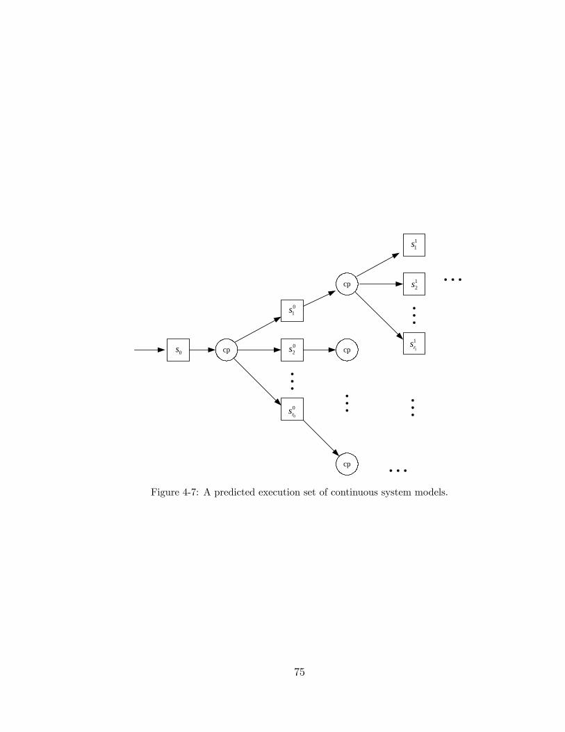
cp
cp
0s
01s
cp
cp
11s
12s
02s
0
0rs
1
1rs
Figure 4-7: A predicted execution set of continuous system models.
75
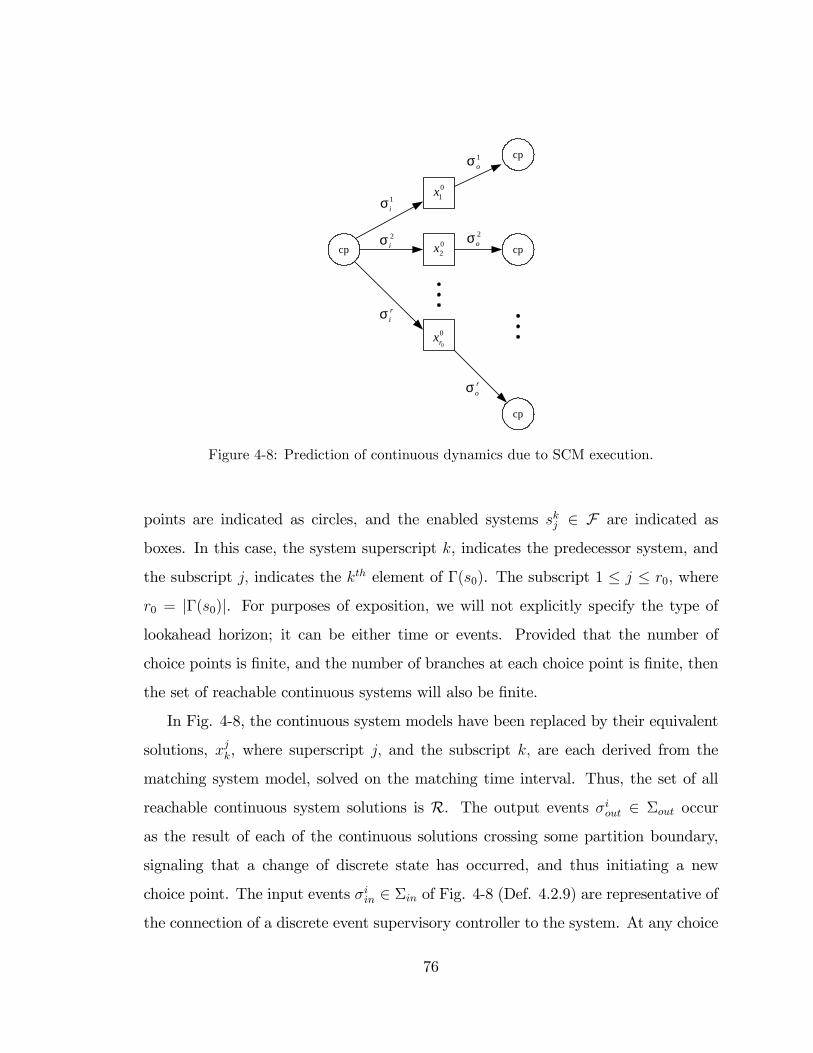
cp
cp
01x
cp
cp
02x
0
0rx
1oσ
2oσ
1iσ
2iσ
roσ
riσ
Figure 4-8: Prediction of continuous dynamics due to SCM execution.
points are indicated as circles, and the enabled systems skj 2 F are indicated as
boxes. In this case, the system superscript k, indicates the predecessor system, and
the subscript j; indicates the kth element of �(s0). The subscript 1 � j � r0, where
r0 = j�(s0)j. For purposes of exposition, we will not explicitly specify the type of
lookahead horizon; it can be either time or events. Provided that the number of
choice points is �nite, and the number of branches at each choice point is �nite, then
the set of reachable continuous systems will also be �nite.
In Fig. 4-8, the continuous system models have been replaced by their equivalent
solutions, xjk, where superscript j; and the subscript k; are each derived from the
matching system model, solved on the matching time interval. Thus, the set of all
reachable continuous system solutions is R. The output events �iout 2 �out occur
as the result of each of the continuous solutions crossing some partition boundary,
signaling that a change of discrete state has occurred, and thus initiating a new
choice point. The input events �iin 2 �in of Fig. 4-8 (Def. 4.2.9) are representative of
the connection of a discrete event supervisory controller to the system. At any choice
76
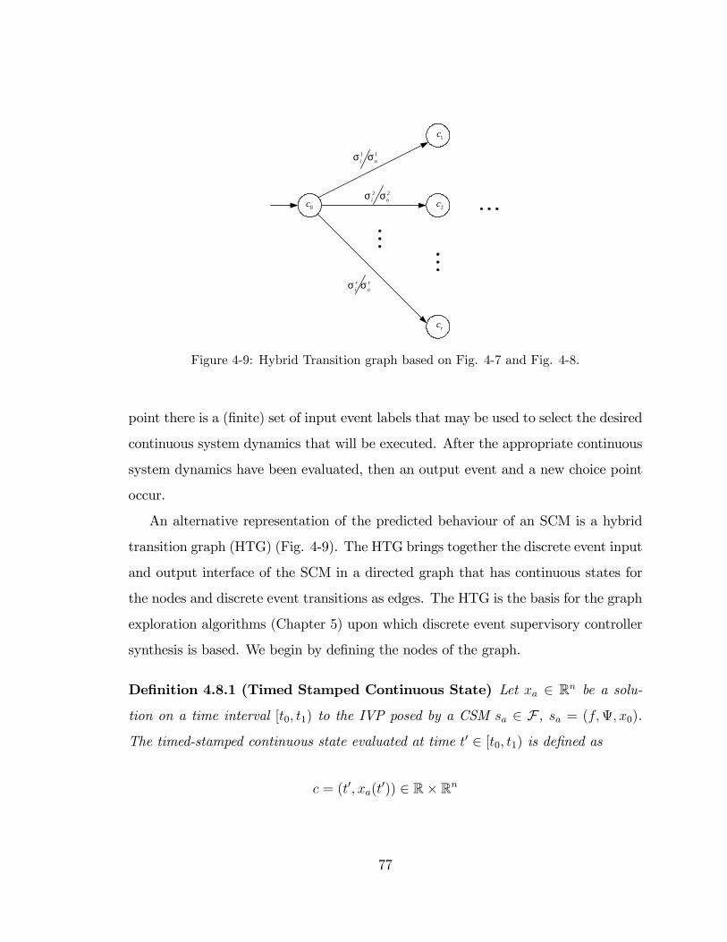
0c
1c
2c
rc
1oσ
2oσ
1iσ
2iσ
roσr
iσ
Figure 4-9: Hybrid Transition graph based on Fig. 4-7 and Fig. 4-8.
point there is a (�nite) set of input event labels that may be used to select the desired
continuous system dynamics that will be executed. After the appropriate continuous
system dynamics have been evaluated, then an output event and a new choice point
occur.
An alternative representation of the predicted behaviour of an SCM is a hybrid
transition graph (HTG) (Fig. 4-9). The HTG brings together the discrete event input
and output interface of the SCM in a directed graph that has continuous states for
the nodes and discrete event transitions as edges. The HTG is the basis for the graph
exploration algorithms (Chapter 5) upon which discrete event supervisory controller
synthesis is based. We begin by de�ning the nodes of the graph.
De�nition 4.8.1 (Timed Stamped Continuous State) Let xa 2 Rn be a solu-
tion on a time interval [t0; t1) to the IVP posed by a CSM sa 2 F , sa = (f;; x0).
The timed-stamped continuous state evaluated at time t0 2 [t0; t1) is de�ned as
c = (t0; xa(t0)) 2 R� Rn
77
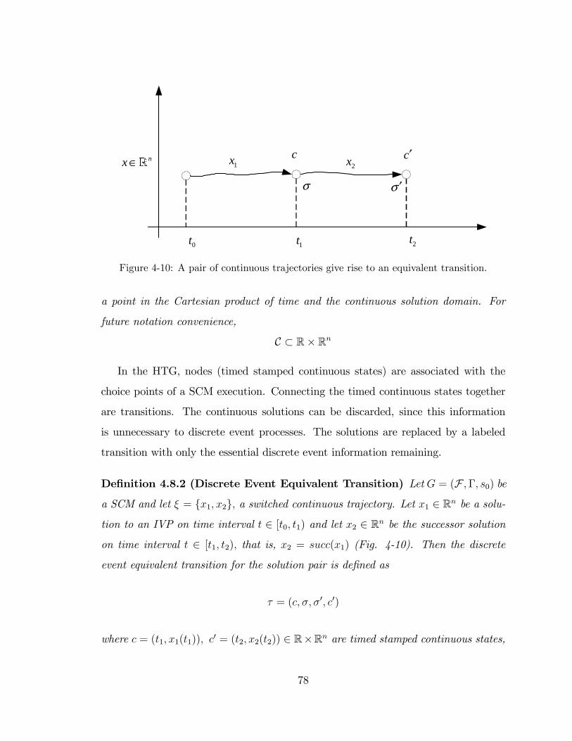
1x 2x
0t
c′c
1t 2t
nx ∈�
σ σ ′
Figure 4-10: A pair of continuous trajectories give rise to an equivalent transition.
a point in the Cartesian product of time and the continuous solution domain. For
future notation convenience,
C � R� Rn
In the HTG, nodes (timed stamped continuous states) are associated with the
choice points of a SCM execution. Connecting the timed continuous states together
are transitions. The continuous solutions can be discarded, since this information
is unnecessary to discrete event processes. The solutions are replaced by a labeled
transition with only the essential discrete event information remaining.
De�nition 4.8.2 (Discrete Event Equivalent Transition) Let G = (F ;�; s0) be
a SCM and let � = fx1; x2g; a switched continuous trajectory. Let x1 2 Rn be a solu-
tion to an IVP on time interval t 2 [t0; t1) and let x2 2 Rn be the successor solution
on time interval t 2 [t1; t2); that is, x2 = succ(x1) (Fig. 4-10). Then the discrete
event equivalent transition for the solution pair is de�ned as
� = (c; �; �0; c0)
where c = (t1; x1(t1)); c0 = (t2; x2(t2)) 2 R�Rn are timed stamped continuous states,
78
the endpoints of the solutions x1 and x2 respectively, and � 2 �in and �0 2 �out are
discrete events.
The input event � 2 �in is the control or input event for the transition. The
output event �0 2 �out occurs as a result of the transition of the continuous solution
into another region (crossing a hypersurface), or as a result of reaching the end of the
designated simulation time interval, �t; in which case the output event is tick. Thus,
the input event can be seen as initiating the occurrence of the output event.
De�nition 4.8.3 (Transition Set) Let G = (F ;�; s0) be a SCM with R the set of
all reachable continuous solutions for some �nite lookahead horizon. The transition
set is the set of all equivalent transitions � 2 TR (Def. 4.8.2, above) corresponding to
all successor pairs of x 2 R
TR = f� : � is an equivalent transition for � = fx; x0g; x; x0 2 R and x0 = succ(x)g
and furthermore, TR � C � �in � �out � C such that
8c 2 C; � 2 �in; jf(�0; c0)j(c; �; �0; c0) 2 TRgj � 1
The transition function and enabled events function may be de�ned in terms of
the transition set.
De�nition 4.8.4 (Transition Function) The transition function �h : C ��in ! C
is de�ned in terms of the transition set TR for c 2 C and � 2 �in:
�h(c; �) =
8<: c0 if 9� = (c; �; �; c0) 2 TRundefined otherwise
where the symbol � indicates a wildcard or �don�t care�event in �out. The domain of
79
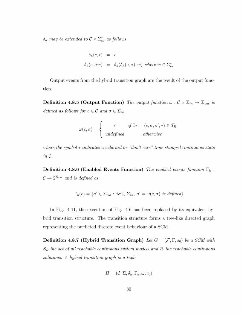
�h may be extended to C � ��in as follows
�h(c; �) = c
�h(c; �w) = �h(�h(c; �); w) where w 2 ��in
Output events from the hybrid transition graph are the result of the output func-
tion.
De�nition 4.8.5 (Output Function) The output function ! : C � �in ! �out is
de�ned as follows for c 2 C and � 2 �in
!(c; �) =
8<: �0 if 9� = (c; �; �0; �) 2 TRunde�ned otherwise
where the symbol � indicates a wildcard or �don�t care�time stamped continuous state
in C.
De�nition 4.8.6 (Enabled Events Function) The enabled events function �h :
C ! 2�out and is de�ned as
�h(c) = f�0 2 �out : 9� 2 �in, �0 = !(c; �) is de�nedg
In Fig. 4-11, the execution of Fig. 4-6 has been replaced by its equivalent hy-
brid transition structure. The transition structure forms a tree-like directed graph
representing the predicted discrete event behaviour of a SCM.
De�nition 4.8.7 (Hybrid Transition Graph) Let G = (F ;�; s0) be a SCM with
SR the set of all reachable continuous system models and R the reachable continuous
solutions. A hybrid transition graph is a tuple
H = (C;�; �h;�h; !; c0)
80
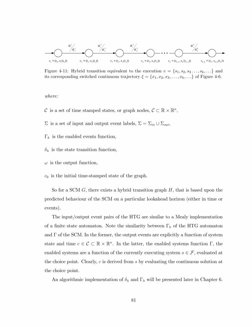
1 0 1 0( , ( ))c t x t= 2 1 2 1( , ( ))c t x t= 3 2 3 2( , ( ))c t x t= 4 3 4 3( , ( ))c t x t= 1 1( , ( ))k k k kc t x t− −= 1 1( , ( ))k k k kc t x t+ +=
1
1i
o
σσ
2
2i
o
σσ
3
3i
o
σσ
ki
ko
σσ
Figure 4-11: Hybrid transition equivalent to the execution v = fs1; s2; s3 : : : ; sk; : : :g andits corresponding switched continuous trajectory � = fx1; x2; x3; : : : ; xk; : : :g of Figure 4-6.
where:
C is a set of time stamped states, or graph nodes, C � R� Rn;
� is a set of input and output event labels, � = �in [ �out;
�h is the enabled events function,
�h is the state transition function,
! is the output function,
c0 is the initial time-stamped state of the graph.
So for a SCM G, there exists a hybrid transition graph H, that is based upon the
predicted behaviour of the SCM on a particular lookahead horizon (either in time or
events).
The input/output event pairs of the HTG are similar to a Mealy implementation
of a �nite state automaton. Note the similarity between �h of the HTG automaton
and � of the SCM. In the former, the output events are explicitly a function of system
state and time c 2 C � R � Rn. In the latter, the enabled systems function �, the
enabled systems are a function of the currently executing system s 2 F , evaluated at
the choice point. Clearly, c is derived from s by evaluating the continuous solution at
the choice point.
An algorithmic implementation of �h and �h will be presented later in Chapter 6.
81
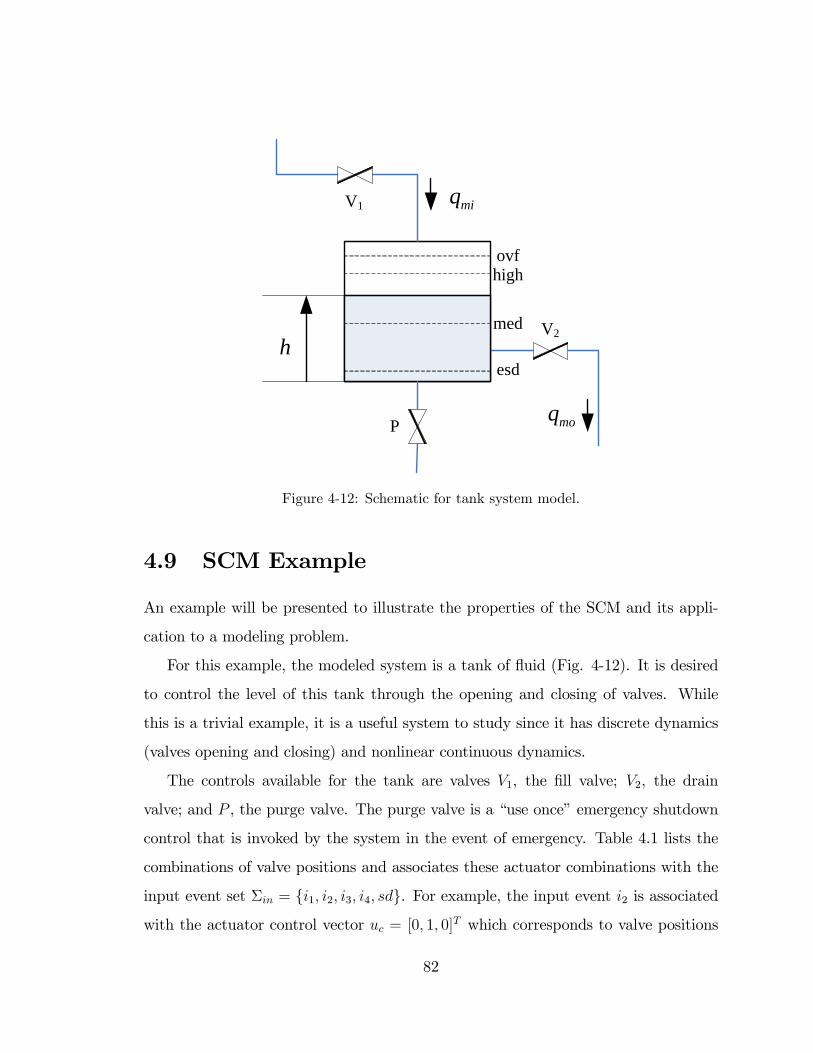
h
miq
moq
ovfhigh
med
esd
V1
V2
P
Figure 4-12: Schematic for tank system model.
4.9 SCM Example
An example will be presented to illustrate the properties of the SCM and its appli-
cation to a modeling problem.
For this example, the modeled system is a tank of �uid (Fig. 4-12). It is desired
to control the level of this tank through the opening and closing of valves. While
this is a trivial example, it is a useful system to study since it has discrete dynamics
(valves opening and closing) and nonlinear continuous dynamics.
The controls available for the tank are valves V1, the �ll valve; V2, the drain
valve; and P , the purge valve. The purge valve is a �use once�emergency shutdown
control that is invoked by the system in the event of emergency. Table 4.1 lists the
combinations of valve positions and associates these actuator combinations with the
input event set �in = fi1; i2; i3; i4; sdg. For example, the input event i2 is associated
with the actuator control vector uc = [0; 1; 0]T which corresponds to valve positions
82
Table 4.1: Valve control structureControl, uc
�in V1 V2 P
i1 0a 0 0i2 0 1 0i3 1 0 0i4 1 1 0sd 0 0 1
aValve open = 1, closed = 0
[V1; V2; P ] = [closed, open, closed]. The shutdown operation is initiated by the input
event sd, which opens only the purge valve to drain the tank. The completion of this
operation is indicated by the esd output event.
The continuous dynamics for the tank can be described by a nonlinear di¤erential
equation. Assume that opening V1 causes a constant mass �ow into the tank qmi,
while opening of V2 or P causes turbulent �ow from the tank. then the general
expression for the tank dynamics (Palm III 2000) is
_h =hqmi �R�1t1
p�gh
�A�R�1t2
p�gh
�A
iuc (4.9)
where h is the liquid level, � is the density of the liquid, and A is the cross sectional
area of the tank. Turbulent resistances for valves V2 and P are Rt1 and Rt2 respec-
tively. The �ve di¤erent actuator control vectors uc, with Eq. 4.9 yield �ve distinct
dynamical models for the tank. Each of these actuator settings along with a set
of state partitioning functionals, forms a separate CSM which will be embedded in
the switched continuous model. For this example, the CSMs corresponding to input
events i1 to i4 share the same set of functionals 1 = fF1; F2; F3; F4g and the CSM for
emergency shutdown operation (purge valve P open) has 2 = fF5g: The functionals
are de�ned in Table 4.2 along with the associated output events.
If the SCM is executed or predicted (Case II switching) on a 90 second time in-
terval, the set of predicted continuous trajectories SR reachable from initial condition
83
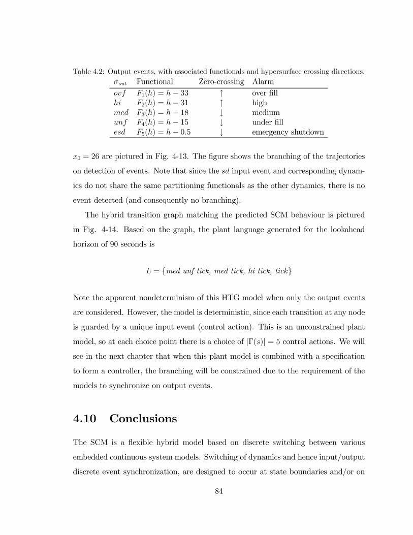
Table 4.2: Output events, with associated functionals and hypersurface crossing directions.�out Functional Zero-crossing Alarmovf F1(h) = h� 33 " over �llhi F2(h) = h� 31 " highmed F3(h) = h� 18 # mediumunf F4(h) = h� 15 # under �llesd F5(h) = h� 0:5 # emergency shutdown
x0 = 26 are pictured in Fig. 4-13. The �gure shows the branching of the trajectories
on detection of events. Note that since the sd input event and corresponding dynam-
ics do not share the same partitioning functionals as the other dynamics, there is no
event detected (and consequently no branching).
The hybrid transition graph matching the predicted SCM behaviour is pictured
in Fig. 4-14. Based on the graph, the plant language generated for the lookahead
horizon of 90 seconds is
L = fmed unf tick, med tick, hi tick, tickg
Note the apparent nondeterminism of this HTG model when only the output events
are considered. However, the model is deterministic, since each transition at any node
is guarded by a unique input event (control action). This is an unconstrained plant
model, so at each choice point there is a choice of j�(s)j = 5 control actions. We will
see in the next chapter that when this plant model is combined with a speci�cation
to form a controller, the branching will be constrained due to the requirement of the
models to synchronize on output events.
4.10 Conclusions
The SCM is a �exible hybrid model based on discrete switching between various
embedded continuous system models. Switching of dynamics and hence input/output
discrete event synchronization, are designed to occur at state boundaries and/or on
84
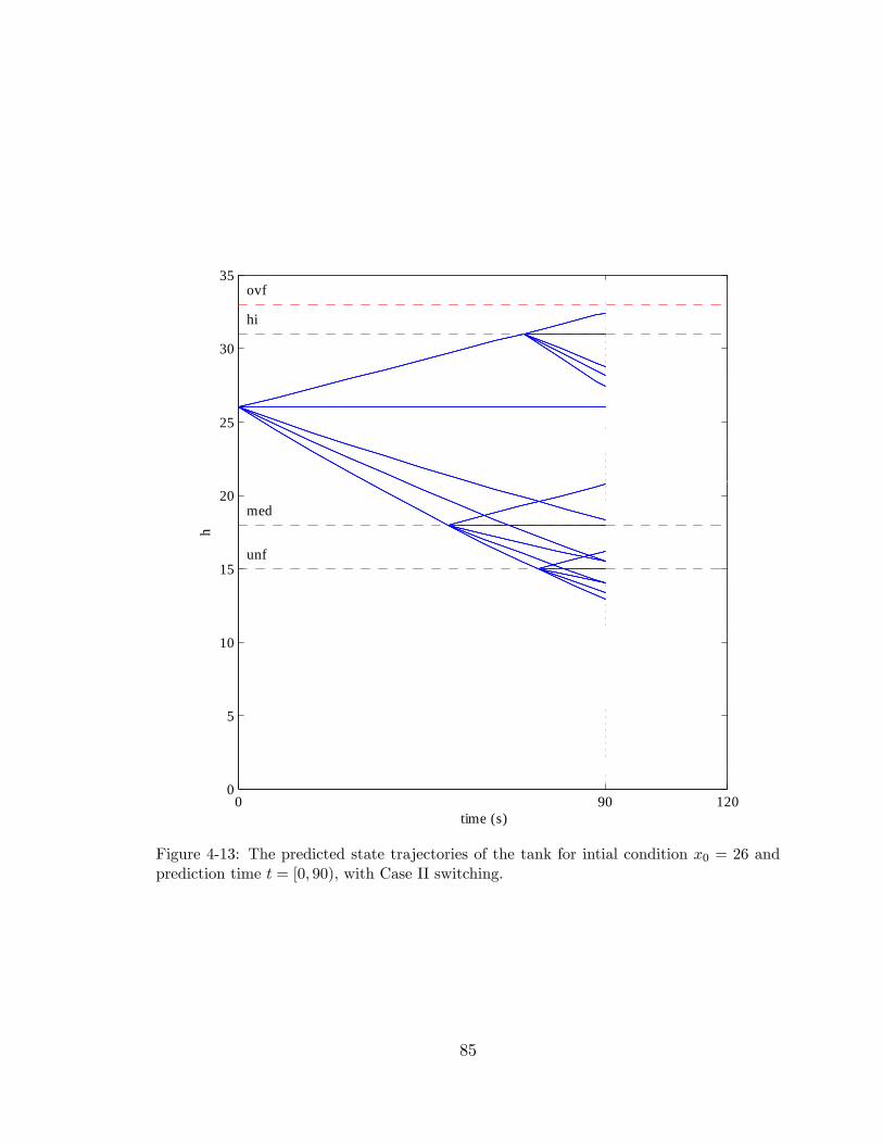
0 90 1200
5
10
15
20
25
30
35
med
unf
hi
ovf
time (s)
h
Figure 4-13: The predicted state trajectories of the tank for intial condition x0 = 26 andprediction time t = [0; 90), with Case II switching.
85

[[0,26]]
[[51.36,18]]
co/med
[[70,31]]oc/hi
[[90,15.5]]sd/tick
[[90,18.37]]
oo/tick
[[90,26]]
cc/tick
[[73.52,15]]
co/unf[[90,14.01]]
sd/tick
[[90,15.49]]oo/tick
[[90,18]]
cc/tick
[[90,20.76]]
oc/tick
[[90,27.4]]co/tick
[[90,28.19]]sd/tick
[[90,28.78]]
oo/tick
[[90,31]]
cc/tick
[[90,32.43]]
oc/tick
[[90,12.95]]
co/tick
[[90,13.4]]sd/tick
[[90,14.08]]oo/tick
[[90,15]]
cc/tick
[[90,16.18]]
oc/tick
Figure 4-14: Hybrid transition graph equivalent for continuous reachable state space of Fig.4-13
86
a synchronous or time-based schedule. Synchronization occurs in both coarse (tick)
and dense time. This is analogous to the operation of industrial control systems in
which a synchronous control cycle is augmented by interrupt-driven control. The
point at which the system switches dynamics is known as a choice point. A �nite set
of enabled systems is available for the system to go forward in time, and one system
is selected to execute. Predicting the future execution of an SCM G = (F ;�; s0)
consists of considering all such enabled systems, extending simulations (solutions) for
each, creating new choice points, and again extending the simulations. Reachability
of the SCM can be expressed in the set of reachable continuous state space solutions
R. The hybrid transition graph captures the discrete-event behaviour of the SCM on
this reachable set. Providing that the SCM has nonzeno behaviour, then the set, and
the HTG will be �nite, and therefore computable.
In the next section, we will examine the process of synthesizing DES supervisory
controllers based on the HTG, which is in essence a discrete event model of the SCM.
87
Chapter5Control of Hybrid Systems
The switched continuous model is a class of hybrid system model. The hybrid
dynamics embodied by this model are characterized by instantaneous switching
between the various embedded continuous dynamical models within the SCM. In order
to control such a process, the controller must act either in the discrete event or the
continuous domain. A DES supervisor has been selected as the most appropriate
tool, since the control objective is to coordinate and sequence the actions of low-
level continuous and discrete event systems that themselves may be controlled or
uncontrolled.
The switching framework of the SCM model has been designed so that it mimics
the intervention of a discrete event supervisory controller, while the output frame-
work is designed to communicate, and thus synchronize, with external discrete event
processes. For purposes of modeling, analysis, and synthesis, it is desirable that the
plant modeled as a SCM may be treated as any other discrete event process.
More complex models may be constructed by forming synchronous products of
switched continuous and �nite state models (FSM). The resulting synchronous prod-
uct behaviour of the product model is similar to the product connection of �nite
state models (FSM). The main di¤erence is that the state space of the SCM is in�-
nite on an in�nite horizon, so that the product connection of FSMs with a SCM has
88
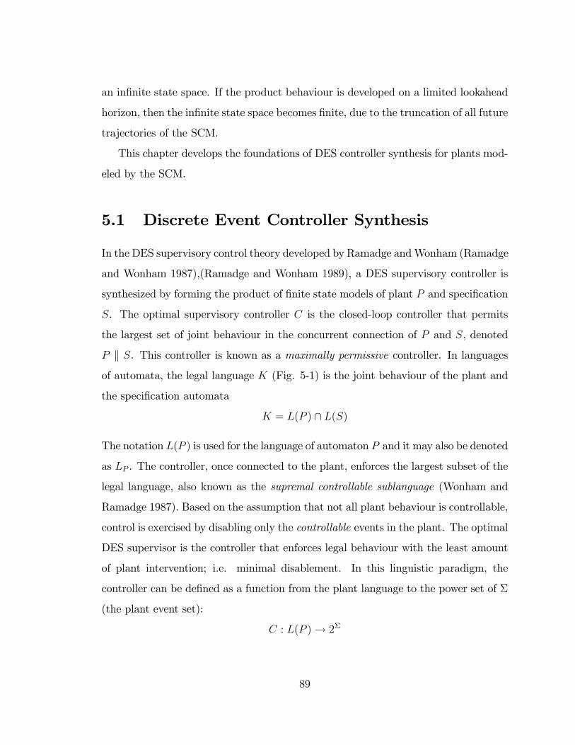
an in�nite state space. If the product behaviour is developed on a limited lookahead
horizon, then the in�nite state space becomes �nite, due to the truncation of all future
trajectories of the SCM.
This chapter develops the foundations of DES controller synthesis for plants mod-
eled by the SCM.
5.1 Discrete Event Controller Synthesis
In the DES supervisory control theory developed by Ramadge andWonham (Ramadge
and Wonham 1987),(Ramadge and Wonham 1989), a DES supervisory controller is
synthesized by forming the product of �nite state models of plant P and speci�cation
S. The optimal supervisory controller C is the closed-loop controller that permits
the largest set of joint behaviour in the concurrent connection of P and S, denoted
P k S. This controller is known as a maximally permissive controller. In languages
of automata, the legal language K (Fig. 5-1) is the joint behaviour of the plant and
the speci�cation automata
K = L(P ) \ L(S)
The notation L(P ) is used for the language of automaton P and it may also be denoted
as LP . The controller, once connected to the plant, enforces the largest subset of the
legal language, also known as the supremal controllable sublanguage (Wonham and
Ramadge 1987). Based on the assumption that not all plant behaviour is controllable,
control is exercised by disabling only the controllable events in the plant. The optimal
DES supervisor is the controller that enforces legal behaviour with the least amount
of plant intervention; i.e. minimal disablement. In this linguistic paradigm, the
controller can be de�ned as a function from the plant language to the power set of �
(the plant event set):
C : L(P )! 2�
89
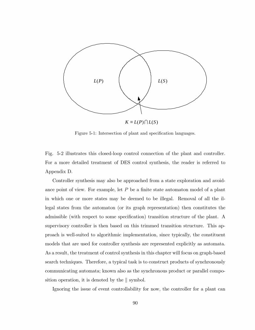
( )L P ( )L S
( ) ( )K L P L S= I
Figure 5-1: Intersection of plant and speci�cation languages.
Fig. 5-2 illustrates this closed-loop control connection of the plant and controller.
For a more detailed treatment of DES control synthesis, the reader is referred to
Appendix D.
Controller synthesis may also be approached from a state exploration and avoid-
ance point of view. For example, let P be a �nite state automaton model of a plant
in which one or more states may be deemed to be illegal. Removal of all the il-
legal states from the automaton (or its graph representation) then constitutes the
admissible (with respect to some speci�cation) transition structure of the plant. A
supervisory controller is then based on this trimmed transition structure. This ap-
proach is well-suited to algorithmic implementation, since typically, the constituent
models that are used for controller synthesis are represented explicitly as automata.
As a result, the treatment of control synthesis in this chapter will focus on graph-based
search techniques. Therefore, a typical task is to construct products of synchronously
communicating automata; known also as the synchronous product or parallel compo-
sition operation, it is denoted by the k symbol.
Ignoring the issue of event controllability for now, the controller for a plant can
90
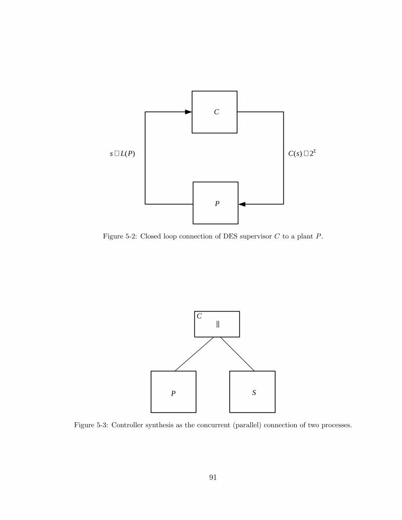
P
C
( )PLs ∈ Σ∈ 2)(sC
Figure 5-2: Closed loop connection of DES supervisor C to a plant P .
S
||
P
C
Figure 5-3: Controller synthesis as the concurrent (parallel) connection of two processes.
91
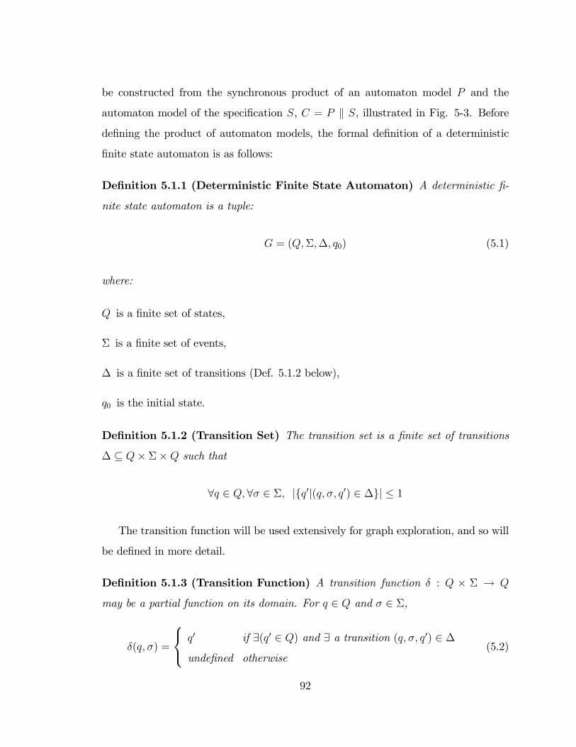
be constructed from the synchronous product of an automaton model P and the
automaton model of the speci�cation S, C = P k S, illustrated in Fig. 5-3. Before
de�ning the product of automaton models, the formal de�nition of a deterministic
�nite state automaton is as follows:
De�nition 5.1.1 (Deterministic Finite State Automaton) A deterministic �-
nite state automaton is a tuple:
G = (Q;�;�; q0) (5.1)
where:
Q is a �nite set of states,
� is a �nite set of events,
� is a �nite set of transitions (Def. 5.1.2 below),
q0 is the initial state.
De�nition 5.1.2 (Transition Set) The transition set is a �nite set of transitions
� � Q� ��Q such that
8q 2 Q;8� 2 �; jfq0j(q; �; q0) 2 �gj � 1
The transition function will be used extensively for graph exploration, and so will
be de�ned in more detail.
De�nition 5.1.3 (Transition Function) A transition function � : Q � � ! Q
may be a partial function on its domain. For q 2 Q and � 2 �,
�(q; �) =
8<: q0 if 9(q0 2 Q) and 9 a transition (q; �; q0) 2 �
unde�ned otherwise(5.2)
92
The domain of � may also be extended to Q� ��. For example,
�(q; �) = q
�(q; �w) = �(�(q; �); w)
For clarity, the function � has domain Q�� and range Q while Eq. 5.2 de�nes the
element to element map. Forthwith, the same convention will be utilized in function
de�nitions.
A second function, known as the enabled events function, is also useful for graph
exploration.
De�nition 5.1.4 (Enabled Events Function) The enabled events function � :
Q! 2� is de�ned as follows
�(q) := f� 2 � : �(q; �) is de�nedg
While inclusion of both � and � in the de�nition of a FSM is redundant, in the
sense that they are already de�ned in terms of the transition set �, they are useful
when de�ning synchronization of multiple automata. In future notation, and for ease
of exposition, �nite state automata will be de�ned in an expanded form as follows:
G = (Q;�; �;�; q0)
Henceforth, the transition set �; will not be explicitly included in the de�nition of
the FSA, since it can be derived from �.
We de�ne the reach operation, which returns the subautomaton that represents
the portion of an automaton that is reachable from its initial state q0.
De�nition 5.1.5 (Reach Operation) Let G = (Q;�; �;�; q0) be a �nite state au-
93
tomaton, then the reach operation is de�ned as follows
reach(G) : = (Qr;�; �r;�; q0) where
Qr = fq 2 Q : 9s 2 ��; �(q0; s) = qg
�r = � on a restricted domain such that Qr � �! Qr
Conceptually, the controller of 5-3, C; is a model-based controller, with models
of the plant and the speci�cation embedded within it. Thus, C is the synchronous
product of �nite state automata (Def. 5.1.1). Throughout this document, the term
�product�will be synonymous with �synchronous product�. Formally, the de�nition
of the synchronous product of two �nite state automata, is as follows:
De�nition 5.1.6 (Product Automaton) Let G1 = (Q1;�1; �1;�1; q01) and G2 =
(Q2;�2; �2;�2; q02) be �nite state automata (see Appendix C for some examples). The
(synchronous) product automaton G1 k G2 is de�ned as
G1k2 = reach(Q1k2;�1k2; �1k2;�1k2; (q01; q02)) (5.3)
where Q1k2 = Q1�Q2 is the Cartesian product of the state sets, �1k2 = �1[�2 is the
union of the event sets, and the product transition function is de�ned in the following
de�nition.
The reach operation in Eq. 5.3 is useful since some parts of the product automaton
may not be reachable from the initial product state (q01; q02), and these portions are
not of interest.
De�nition 5.1.7 (Product Transition Function) Let G1 and G2 be �nite state
automata (Def. 5.1.6), then their product transition function
�1k2 : (Q1 �Q2)� (�1 [ �2)! (Q1 �Q2)
94
�1k2((q1; q2); �) =
8>>>>>><>>>>>>:
(�1(q1; �); �2(q2; �)) if � 2 �1(q1) \ �2(q2)
(�1(q1; �); q2) if � 2 �1(q1)n�2(q1; �2(q2; �)) if � 2 �2(q2)n�1unde�ned otherwise
Note that �1k2 like �1 and �2, is a partial function.
De�nition 5.1.8 The product enabled events function
�1k2 : (Q1 �Q2)! 2(�1\�2)
�1k2(q1; q2) = [�1(q1) \ �2(q2)] [ [�1(q1) \ (�1 n �2)] [ [�2(q2) \ (�2 n �1)] (5.4)
The �rst term of Eq. 5.4 requires that events common to both enabled events
functions �1 and �2 (and hence common to the event sets of both automata) must be
synchronized. The latter two terms are the sets of enabled events that are private to
each of the automata; there is no requirement for these to be synchronized, so they will
always be included. The synchronous product operation of automata is associative
(Cassandras and Lafortune 1999). The associative property permits the product
automaton operation of Def. 5.1.6 to be extended easily to an n-ary product, in which
n automata are synchronized. Associativity also permits the hierarchical nesting of
synchronous product operations. This modularity lends itself naturally, as we shall
see later, to an object oriented programming implementation. Hierarchical modeling
also allows for a �exible modeling scheme in which automata may be grouped by their
functional relevance to each other; e.g. the sub-automata that form a speci�cation
and the sub-automata that form a plant. Fig. 5-4 is an example of a hierarchical
model of the discrete event behaviour of a ship�s power and propulsion systems. In this
example, each of the various subsystem models are grouped as functionally related
components. For example, the power system behaviour is modeled as a product of
the two product automata, Generator #1 and Generator #2. A ��at�equivalent to
95

product
Power
product
Generator #1
product
Generator #2
Electrical Mechanical Electrical Mechanical
Thruster 1 Thruster 2 Thruster 3
product
Propulsion
product
Ship
Figure 5-4: Hypothetical hierarchical automaton model for a ship�s propulsion and powergeneration subsystems..
this hierarchical model may be constructed by taking the lowermost (non-product)
components of the tree and placing them in a single-level product automaton.
Synthesis of a DES controller in the SCM environment requires the construction
of synchronous product structures of SCMs and �nite state models. The discrete
event interface that was developed for the SCM in the previous chapter allows these
product structures to be constructed. This is the basis of DES supervisory controller
synthesis for hybrid systems.
5.2 SCM and Control Synthesis
Suppose that we have a SCM P , that models the dynamics of a plant and a timed
FSM, S that models a speci�cation. In our framework, controller synthesis consists
of the synchronous product of the plant and speci�cation models. In §4.8, the hybrid
transition graph was introduced as a representation of the discrete event dynamics
for a SCM. In addition, on a �nite event or time horizon, the HTG is of �nite size.
Now we de�ne a new transition structure which encapsulates the synchronous
product of an HTG and a FSM where the state of this structure is the product state
96

of the respective states of the HTG and the FSM. The product of a hybrid transition
graph and a �nite state automaton is de�ned as follows.
De�nition 5.2.1 (Hybrid Product Automaton) LetH = (C;�h; �h;�h; !; c0) be
a hybrid transition graph and G = (Q;�g; �g;�g; q0) be a �nite state automaton, the
product automaton is de�ned as
H k G = reach(C �Q;�h [ �g; �hkg;�hkg; !; (c0; q0))
with �hkg and �hkg as de�ned below.
Note that the transition set TR can be omitted from the HTG de�nition, since �h
and �h can provide the same information set. States of a hybrid product automaton
(HPA) are truly hybrid by the usual de�nitions of a hybrid system, since the state has
both a continuous and discrete state component. Note also that the product states
of the HPA H k G inherit the time stamps of the HTG. The inclusion of time within
the state of the product automaton also ensures that the resulting product graph will
be acyclic.
The objective of the modeling framework is to achieve a �nite state representation.
By making the assumption that the event set of G, �g � �out, then the set of events
�g(q)n�out = ;. This means that events are generated by the SCM only, and the
�nite state machine G acts as an acceptor. For control synthesis, H is the plant
model and G is either a model of the speci�cation, or part of the plant model, so this
is a reasonable assumption. Since H generates the output events via the output event
function, only the shaded set(s) illustrated in Fig. 5-5 are necessary to consider for
the transition function.
De�nition 5.2.2 ( HPA Transition Function) Let �h = �in [ �out, then
�hkg : (C �Q)� �in ! (C �Q)
97
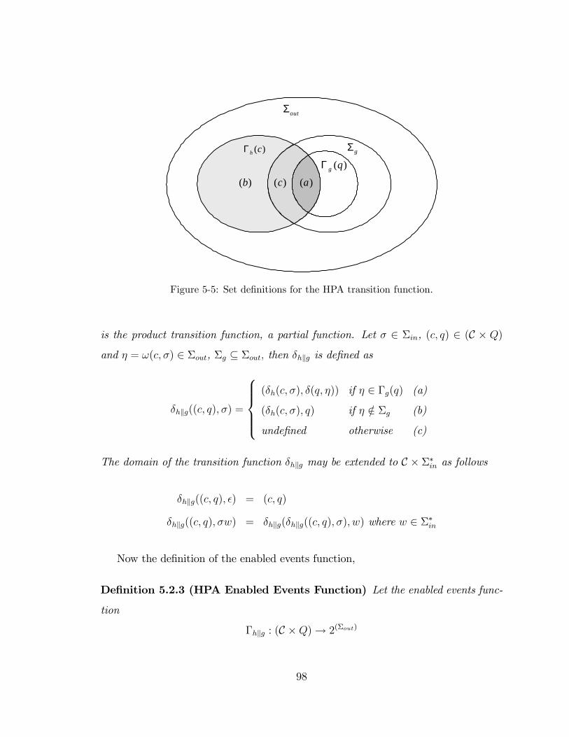
outΣ
( )h cΓ
( )g qΓgΣ
( )a( )b ( )c
Figure 5-5: Set de�nitions for the HPA transition function.
is the product transition function, a partial function. Let � 2 �in, (c; q) 2 (C � Q)
and � = !(c; �) 2 �out, �g � �out; then �hkg is de�ned as
�hkg((c; q); �) =
8>>><>>>:(�h(c; �); �(q; �)) if � 2 �g(q) (a)
(�h(c; �); q) if � =2 �g (b)
unde�ned otherwise (c)
The domain of the transition function �hkg may be extended to C � ��in as follows
�hkg((c; q); �) = (c; q)
�hkg((c; q); �w) = �hkg(�hkg((c; q); �); w) where w 2 ��in
Now the de�nition of the enabled events function,
De�nition 5.2.3 (HPA Enabled Events Function) Let the enabled events func-
tion
�hkg : (C �Q)! 2(�out)
98
If c 2 C and q 2 Q, then
�hkg(c; q) = [�h(c)n�g] [ [�h(c) \ �g(q)]
From these de�nitions, it is apparent that the HTG automaton synchronizes only
its output events with the events of the �nite state automaton. The intent here is
to mimic the standard synchronization technique that is used in DES supervisory
synthesis. The focus is placed on the plant�s discrete event behaviour which is com-
municated by the output events. Speci�cations are normally written in terms of the
desired (output) dynamics, thus the synchronization of output events is a practical
modeling decision.
Input events are not synchronized; these represent the actions that are available
to the controller. Later, we will see that a control choice mechanism selects one
� 2 �in as the control action. The result of the selection of a particular input event
leads to the generation of an output event, when the underlying continuous system
dynamics transition to a new discrete state. So in e¤ect, synchronization of output
events causes certain input events to be ineligible implicitly. An improvement to the
SCM framework would be to include explicit input synchronization. For example,
SC models could have a �nite state �front-end�, permitting the set of enabled input
events (viable control actions) to be a function of the state of the front-end automaton.
Finally, we will look at the synchronization of SCMs with each other. It may
be desirable to approach the modeling of the continuous dynamics of a system in
a modular fashion. If the continuous dynamics are separated into multiple SCMs,
they may be synchronized at the discrete event level. Since dense time information is
available from each of the HTG processes, it is possible to detect the �earliest�event
that occurs amongst them; this becomes a new state in the product by evaluating the
solutions of each of the other systems at this event time.
An alternative approach to synchronization of SCMs at the discrete event level,
is to lump all continuous state variables into a single set of continuous models, and
99
embed these into a single SCM. The choice is left up to the designer; if the continu-
ous dynamics have signi�cant coupling, then communicating state variables are best
lumped together. If the continuous dynamics are coupled through indirect discrete
event communication, then they may be modeled more e¤ectively as separate SCMs.
An algorithm that implements multiple SCM object synchronization will be presented
in chapter 6.
5.2.1 Example: Product of SCM and FSM
To illustrate the synchronous product operation, we will revisit the SCM tank mod-
eling example of §4.9. The HTG that results from this example models the discrete
event behaviour of the uncontrolled tank for a 90 second lookahead horizon (recall
Fig.4-14, p. 86). Let the �nite state model of the speci�cation
S = (Q;�s; �;�; q0)
�s = fhi, tick, unfg:
The plant graph is presented again in Fig.5-6, along with the speci�cation The plant
model �inherits�its output event set from the switched continuous model. In Table
4.2 (p. 84), recall that the SCM output events are
�out = fovf, hi, med, unf, esdg [ ftickg
and the input event set is
�in = foo, oc, co, cc, sdg
The resulting product P k S , illustrates how the original plant graph is modi�ed by
the product connection of the speci�cation (Fig. 5-6, bottom). Starting with the ini-
tial state of the plant, c0 = [0; 26] 2 (R�R), �P (c0) = ftick, hi, medg, all transitions
100
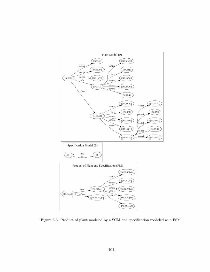
Product of Plant and Specification (P||S)
Specification Model (S)
Plant Model (P)
[[0,26],q0]
[[51.36,18],q0]
co/med
[[70,31],q1]oc/hi
[[90,27.4],q0]
co/tick[[90,28.19],q0]
sd/tick[[90,28.78],q0]oo/tick
[[90,31],q0]cc/tick
[[90,32.43],q0]
oc/tick
q0 q1hi
tick
[[0,26]]
[[51.36,18]]
co/med
[[70,31]]
oc/hi[[90,15.5]]sd/tick
[[90,18.37]]oo/tick
[[90,26]]
cc/tick
[[73.52,15]]
co/unf
[[90,14.01]]
sd/tick [[90,15.49]]
oo/tick
[[90,18]]cc/tick
[[90,20.76]]oc/tick
[[90,27.4]]
co/tick[[90,28.19]]sd/tick
[[90,28.78]]oo/tick
[[90,31]]
cc/tick
[[90,32.43]]
oc/tick
[[90,12.95]]co/tick
[[90,13.4]]sd/tick
[[90,14.08]]oo/tick
[[90,15]]cc/tick
[[90,16.18]]oc/tick
Figure 5-6: Product of plant modeled by a SCM and speci�cation modeled as a FSM.
101
with tick output events are removed from the graph because (tick =2 �S(q0)). The tran-
sition having output event hi remains because it synchronizes with the speci�cation.
The transition with output event med remains in the product because (med =2 �s).
The process of trimming continues until each remaining (and reachable) state in the
product graph has been visited.
Starting from the initial state of the product automaton (the root of the tree),
there exist 6 unique branches. Of these six branches, one ends in a product state
c = [[51:36; 18]; q0] 2 ((R � R) � Q). The time of the continuous product state is
t = 51:36; which is less than the lookahead horizon. Since this branch does not take
the system to the simulation horizon, it is not a viable choice for a controller to
make, since the system cannot safely continue on this trajectory to the horizon. This
concept will be elaborated upon in the next section. The viable controller actions for
this plant, at this time, are the set of input strings
L(C) = foc oc, oc cc, oc oo, oc sd, oc co}
5.3 Blocking
In standard DES supervisory control theory, the concept of controller blocking is
de�ned in the context that certain states have a special status; i.e. marked states. In
the DES framework, if an automaton reaches a state that is not marked, and � = ;,
it is said to be deadlocked or blocked. Supervisory controllers are designed to be both
safe and nonblocking.
In a system model based on a SCM, the concept of blocking is de�ned di¤erently
from the typical DES de�nition. In the SCM framework there is a richer set of
information, particularly the fact that dense-time state (and event) information is
available. Having the knowledge of the time at which the system has entered a
state (the time stamp of the HTG states) allows us to de�ne blocking in terms of the
terminal state time. The system has the extra dimension of time to de�ne the progress
102
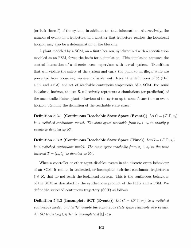
(or lack thereof) of the system, in addition to state information. Alternatively, the
number of events in a trajectory, and whether that trajectory reaches the lookahead
horizon may also be a determination of the blocking.
A plant modeled by a SCM, on a �nite horizon, synchronized with a speci�cation
modeled as an FSM, forms the basis for a simulation. This simulation captures the
control interaction of a discrete event supervisor with a real system. Transitions
that will violate the safety of the system and carry the plant to an illegal state are
prevented from occurring, via event disablement. Recall the de�nitions of R (Def.
4.6.2 and 4.6.3), the set of reachable continuous trajectories of a SCM. For some
lookahead horizon, the set R collectively represents a simulations (or prediction) of
the uncontrolled future plant behaviour of the system up to some future time or event
horizon. Re�ning the de�nition of the reachable state space:
De�nition 5.3.1 (Continuous Reachable State Space (Events)) Let G = (F ;�; s0)
be a switched continuous model. The state space reachable from x0 2 s0 in exactly p
events is denoted as Rp.
De�nition 5.3.2 (Continuous Reachable State Space (Time)) Let G = (F ;�; s0)
be a switched continuous model. The state space reachable from x0 2 s0 in the time
interval T = (t0; tf ] is denoted as RT .
When a controller or other agent disables events in the discrete event behaviour
of an SCM, it results in truncated, or incomplete, switched continuous trajectories
� 2 R, that do not reach the lookahead horizon. This is the continuous behaviour
of the SCM as described by the synchronous product of the HTG and a FSM. We
de�ne the switched continuous trajectory (SCT) as follows
De�nition 5.3.3 (Incomplete SCT (Events)) Let G = (F ;�; s0) be a switched
continuous model, and let Rp denote the continuous state space reachable in p events.
An SC trajectory � 2 Rp is incomplete if j�j < p.
103
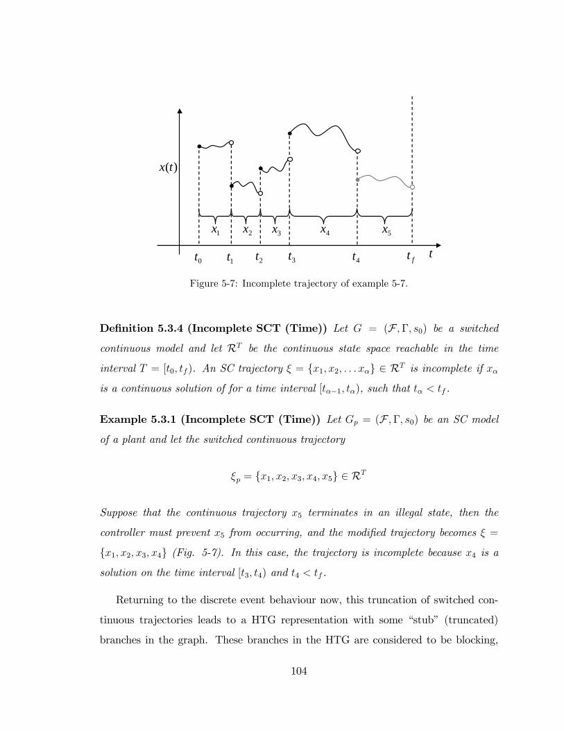
1x 2x 3x 4x 5x
0t t
)(tx
1t 2t 3t 4t ft
Figure 5-7: Incomplete trajectory of example 5-7.
De�nition 5.3.4 (Incomplete SCT (Time)) Let G = (F ;�; s0) be a switched
continuous model and let RT be the continuous state space reachable in the time
interval T = [t0; tf ). An SC trajectory � = fx1; x2; : : : x�g 2 RT is incomplete if x�is a continuous solution of for a time interval [t��1; t�), such that t� < tf .
Example 5.3.1 (Incomplete SCT (Time)) Let Gp = (F ;�; s0) be an SC model
of a plant and let the switched continuous trajectory
�p = fx1; x2; x3; x4; x5g 2 RT
Suppose that the continuous trajectory x5 terminates in an illegal state, then the
controller must prevent x5 from occurring, and the modi�ed trajectory becomes � =
fx1; x2; x3; x4g (Fig. 5-7). In this case, the trajectory is incomplete because x4 is a
solution on the time interval [t3; t4) and t4 < tf .
Returning to the discrete event behaviour now, this truncation of switched con-
tinuous trajectories leads to a HTG representation with some �stub� (truncated)
branches in the graph. These branches in the HTG are considered to be blocking,
104

since it is not possible to �nd a path (trajectory) from the initial state to the lookahead
horizon. In the following de�nitions, for clarity, we consider the only the legal behav-
iour of HTGs, assuming that synchronization with an external process has already
enforced legal behaviour (a speci�cation for example).
De�nition 5.3.5 (Blocking & Nonblocking States (Time Horizon)) LetH be
a hybrid transition graph based on a time T = [t0; tf ) reach of the SCM G. Let H
have initial state c0 = (t0; x(t0)) 2 R� Rn and let c0 = (t0; x(t0)) 2 R� Rn be a time
stamped continuous state in the graph H such that �h(c0) = ;. If there exists a string
u 2 ��in such that �h(c0; u) = c0, and if t0 < tf , then state c0 is blocking. Conversely,
if t0 = tf , then state c0 is nonblocking.
De�nition 5.3.6 (Blocking & Nonblocking States (Event Horizon)) LetH be
a hybrid transition graph based on a reach of p events of the SCM G. Let H have
initial time stamped state c0 = (t0; x(t0)) 2 R�Rn and let c0 = (t0; x(t0)) 2 R�Rn be a
state such that �h(c0) = ;. If there exists a string u 2 ��in such that �h(c0; u) = c0 and
juj < p; then c0 is a blocking state. Conversely, if juj = p, then state c0 is nonblocking.
To illustrate blocking, we start with the HTG H of Fig. 5-8, a plant model of
a system. For purposes of exposition, the graph is the unrestricted (uncontrolled)
SCM behaviour. We will assume that there exists a FSA S, as an acceptor, that
models the speci�cation. It supplies the state marking by labeling the continuous
states as illegal if the discrete-event language of the plant H, falls outside of the legal
behaviour speci�ed by S. Therefore, all continuous trajectories of this system are
complete, either in time or events; that is, states c1 through c8 are at the lookahead
horizon. In the continuous state of the SCM, any path traversing the graph from
the initial state c0 to one of these end states corresponds to a complete switched
continuous trajectory. Illegal states are indicated as grey-coloured nodes, c3, c4; c5;
and c9 (marked by the speci�cation acceptor automaton). To enforce safety, these
nodes must be removed from the graph, with the result indicated in Fig. 5-9.
105
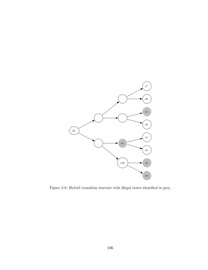
c0
b1
b2
b4
b3
c7
c8
c5
c6
c9
c10
c1
c2
c3
c4
Figure 5-8: Hybrid transition stucture with illegal states identi�ed in grey.
106
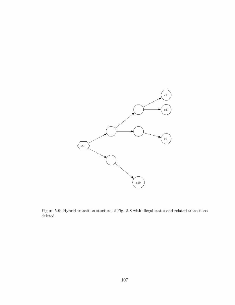
c0
b1
b2
b4
b3
c7
c8
c6
c10
Figure 5-9: Hybrid transition stucture of Fig. 5-8 with illegal states and related transitionsdeleted.
107
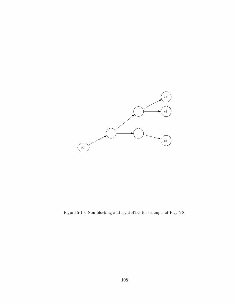
c0
b1
b4
b3
c7
c8
c6
Figure 5-10: Non-blocking and legal HTG for example of Fig. 5-8.
108
In the case of states c1 and c2; they cannot be reached without traversing an
illegal state, c9 �rst. Removing c9 and the transition that enters it, makes c1 and
c2 unreachable, and therefore they are not viable. States c3 and c4; although on the
lookahead horizon, are illegal. Removing these states leaves a stub branch in the HTG
at state c10, which is a blocking state. The blocking trajectory that ends with c10
must be removed from the graph. By examination, all states and transitions of this
branch will have to be pruned back to the initial state in order to avoid blocking. The
result is illustrated in Fig. 5-10, which retains three possible legal and nonblocking
trajectories, taking the system from c0 to c6, c7 and c8.
5.4 Fail-safe Controller Operation
As we have seen in the previous sections, a product of a HTG and one or more
�nite state models is the basis for the DES controller. Appropriate trimming of
states and transitions from the HTG yields a controller graph that represents the
safe and nonblocking controller actions, given the limited horizon of knowledge that
is available. In previous limited lookahead work (Chung et al. 1992) the set of safe
actions or trajectories, are known as pending traces. This set of legal control actions
is further re�ned by taking either an optimistic or conservative policy with respect to
the expected behaviour of the system beyond the current lookahead horizon. With an
optimistic policy (or outlook), all pending traces are assumed to have continuations
beyond the lookahead horizon that are both legal and marked. In the case of the
conservative policy however, all trajectories are assumed to continue uncontrollably
into illegal or blocking conditions. These attitudes condition how the set of pending
traces is further re�ned. The farther the lookahead horizon is extended, the less
ambiguity there is about the pending traces.
An online controller algorithm must have a means of selecting the next control
action. The ultimate objective of this controller is to drive the system from the initial
109
state to the lookahead horizon without violating the safety.
De�nition 5.4.1 (Nonblocking Controller) Let H be the HTG of a system mod-
eled by SCM G having only legal states, and an initial time stamped state c0 =
(t0; x(t0)) 2 R � Rn.The system has a nonblocking safe controller if there exists at
least one nonblocking state c0 and there exists a control string u 2 ��in, such that
c0 = �h(c0; u).
Again, we have examined H in isolation. The assumption is that SCM G is
synchronized with an external process, ensuring only legal states exist.
But what happens if the system arrives at a state from which only blocking tra-
jectories exist? In the absence of a legal control choice, the system must continue
(since time cannot be stopped), and since only illegal choices remain, the controller
will be forced to proceed with a control action that ultimately violates the system
safety. Hence, nonblocking is equivalent to safety. Unfortunately, there can never be
a guarantee that just beyond the lookahead horizon, the controller might block, and
a safety violation will be forced. We would like to design a controller for this online
discrete event environment which can be guaranteed to be free of this sort of forced
safety violations.
5.4.1 Emergency Shutdown
A standard design practice in safety critical industrial control is to incorporate an
emergency shutdown (ESD) mechanism into the control system. It is generally con-
sidered good design practice to include some sort of fail-safe subsystem in controlled
systems at design time. Examples of industries that utilize such fail-safe mechanisms
as part of the control infrastructure include:
� Oil and Gas Processing
� Nuclear Power Generation
110
� Chemical Manufacturing
� Transportation (Rail Transit)
� Motion Control
Terms for fail-safe control procedures vary by industry, but examples are emer-
gency shut down (ESD), from Oil and Gas processing applications, emergency stop
(E-Stop), from motion control applications and the SCRAM procedure for nuclear
reactors. In order to model the emergency shutdown behaviour, it is necessary to
de�ne what is meant in a discrete-event sense as an ESD.
De�nition 5.4.2 (Emergency Shutdown State Set) LetH = (C;�; �h;�h; !; c0)
be a HTG of SCM G = (F ;�; s0). The emergency shutdown state set E � C such
that
E = fc : �(c) = ftickg and �(c; �) 2 E; 8� 2 �ing
An element c 2 E is an emergency shutdown state.
Obviously, an ESD state should be considered by a DES controller as a safe state;
the ESD states can be identi�ed (or marked) by synchronization of additional FSM
plant model when designing the controller. In the context of the continuous behaviour
of the switched continuous model, an ESD state might be abstractly interpreted as a
Lyapunov-stable equilibrium (see Appendix A) within one or more of the CSMs. If a
continuous trajectory of the system can enter such a Lyapunov stable region, it will be
�captured�, remaining within a de�ned region. If the region has been partitioned ap-
propriately, any trajectory entering the region will fail to generate events (other than
tick), since no partition boundaries are crossed. Thus, an emergency shutdown region
is de�ned in terms of (stable) dynamics and an appropriate partitioning boundary.
While it is undesirable to enter an ESD state from the point of view that it
performs no useful work, it is preferable to a potentially catastrophic safety violation.
111
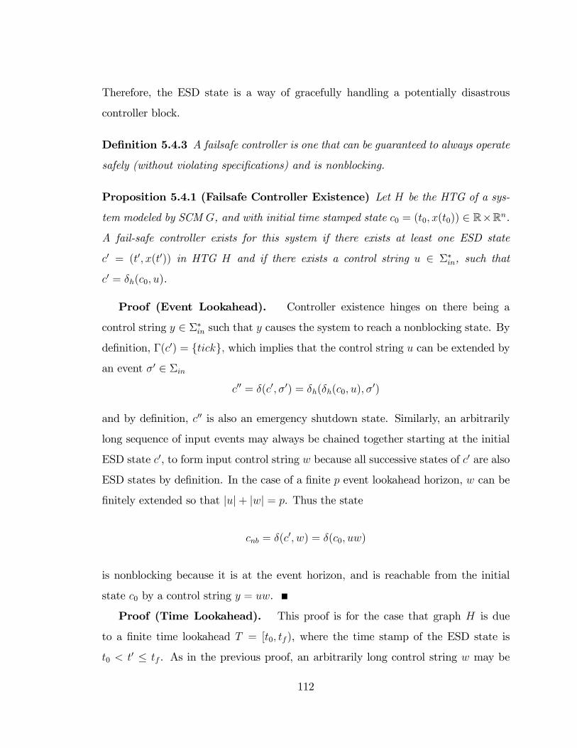
Therefore, the ESD state is a way of gracefully handling a potentially disastrous
controller block.
De�nition 5.4.3 A failsafe controller is one that can be guaranteed to always operate
safely (without violating speci�cations) and is nonblocking.
Proposition 5.4.1 (Failsafe Controller Existence) Let H be the HTG of a sys-
tem modeled by SCM G, and with initial time stamped state c0 = (t0; x(t0)) 2 R�Rn.
A fail-safe controller exists for this system if there exists at least one ESD state
c0 = (t0; x(t0)) in HTG H and if there exists a control string u 2 ��in, such that
c0 = �h(c0; u).
Proof (Event Lookahead). Controller existence hinges on there being a
control string y 2 ��in such that y causes the system to reach a nonblocking state. By
de�nition, �(c0) = ftickg; which implies that the control string u can be extended by
an event �0 2 �inc00 = �(c0; �0) = �h(�h(c0; u); �
0)
and by de�nition, c00 is also an emergency shutdown state. Similarly, an arbitrarily
long sequence of input events may always be chained together starting at the initial
ESD state c0, to form input control string w because all successive states of c0 are also
ESD states by de�nition. In the case of a �nite p event lookahead horizon, w can be
�nitely extended so that juj+ jwj = p. Thus the state
cnb = �(c0; w) = �(c0; uw)
is nonblocking because it is at the event horizon, and is reachable from the initial
state c0 by a control string y = uw.
Proof (Time Lookahead). This proof is for the case that graph H is due
to a �nite time lookahead T = [t0; tf ), where the time stamp of the ESD state is
t0 < t0 � tf . As in the previous proof, an arbitrarily long control string w may be
112
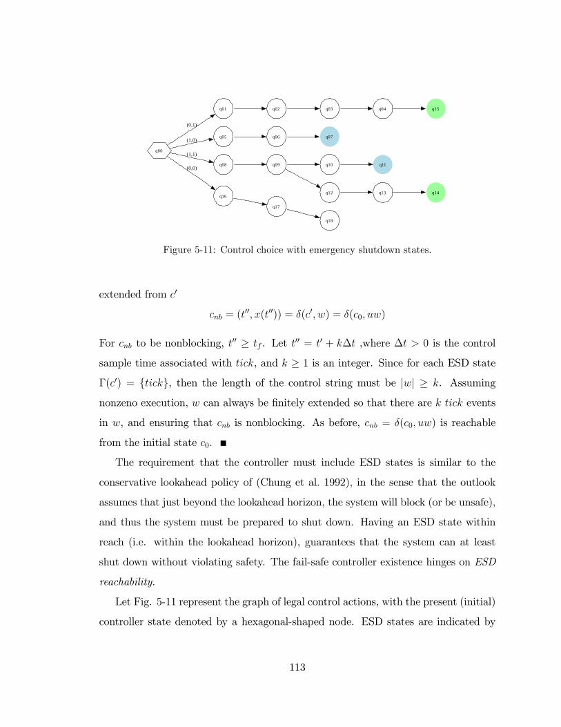
q00
q01
(0,1)
q05(1,0)
q08
(1,1)
q16
(0,0)
q02 q03 q04 q15
q06 q07
q09 q10
q12
q11
q13 q14
q17
q18
Figure 5-11: Control choice with emergency shutdown states.
extended from c0
cnb = (t00; x(t00)) = �(c0; w) = �(c0; uw)
For cnb to be nonblocking, t00 � tf . Let t00 = t0 + k�t ,where �t > 0 is the control
sample time associated with tick, and k � 1 is an integer. Since for each ESD state
�(c0) = ftickg, then the length of the control string must be jwj � k. Assuming
nonzeno execution, w can always be �nitely extended so that there are k tick events
in w, and ensuring that cnb is nonblocking. As before, cnb = �(c0; uw) is reachable
from the initial state c0.
The requirement that the controller must include ESD states is similar to the
conservative lookahead policy of (Chung et al. 1992), in the sense that the outlook
assumes that just beyond the lookahead horizon, the system will block (or be unsafe),
and thus the system must be prepared to shut down. Having an ESD state within
reach (i.e. within the lookahead horizon), guarantees that the system can at least
shut down without violating safety. The fail-safe controller existence hinges on ESD
reachability.
Let Fig. 5-11 represent the graph of legal control actions, with the present (initial)
controller state denoted by a hexagonal-shaped node. ESD states are indicated by
113
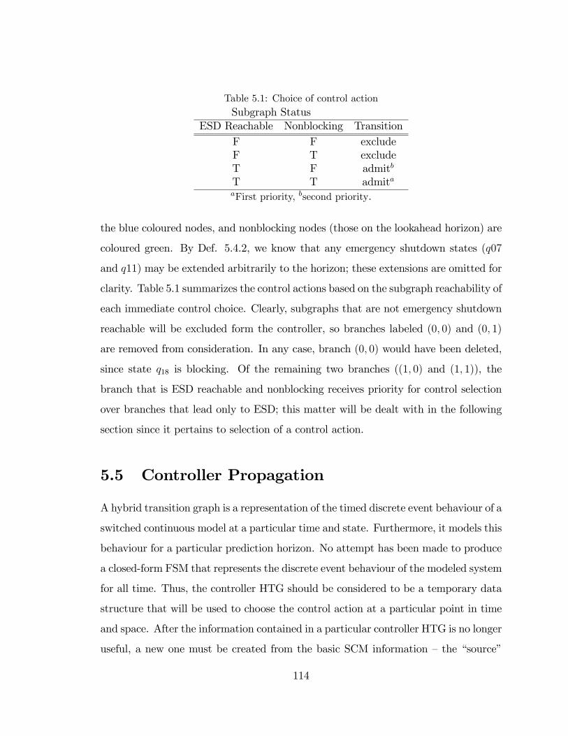
Table 5.1: Choice of control actionSubgraph Status
ESD Reachable Nonblocking TransitionF F excludeF T excludeT F admitb
T T admitaaFirst priority, bsecond priority.
the blue coloured nodes, and nonblocking nodes (those on the lookahead horizon) are
coloured green. By Def. 5.4.2, we know that any emergency shutdown states (q07
and q11) may be extended arbitrarily to the horizon; these extensions are omitted for
clarity. Table 5.1 summarizes the control actions based on the subgraph reachability of
each immediate control choice. Clearly, subgraphs that are not emergency shutdown
reachable will be excluded form the controller, so branches labeled (0; 0) and (0; 1)
are removed from consideration. In any case, branch (0; 0) would have been deleted,
since state q18 is blocking. Of the remaining two branches ((1; 0) and (1; 1)), the
branch that is ESD reachable and nonblocking receives priority for control selection
over branches that lead only to ESD; this matter will be dealt with in the following
section since it pertains to selection of a control action.
5.5 Controller Propagation
A hybrid transition graph is a representation of the timed discrete event behaviour of a
switched continuous model at a particular time and state. Furthermore, it models this
behaviour for a particular prediction horizon. No attempt has been made to produce
a closed-form FSM that represents the discrete event behaviour of the modeled system
for all time. Thus, the controller HTG should be considered to be a temporary data
structure that will be used to choose the control action at a particular point in time
and space. After the information contained in a particular controller HTG is no longer
useful, a new one must be created from the basic SCM information �the �source�
114
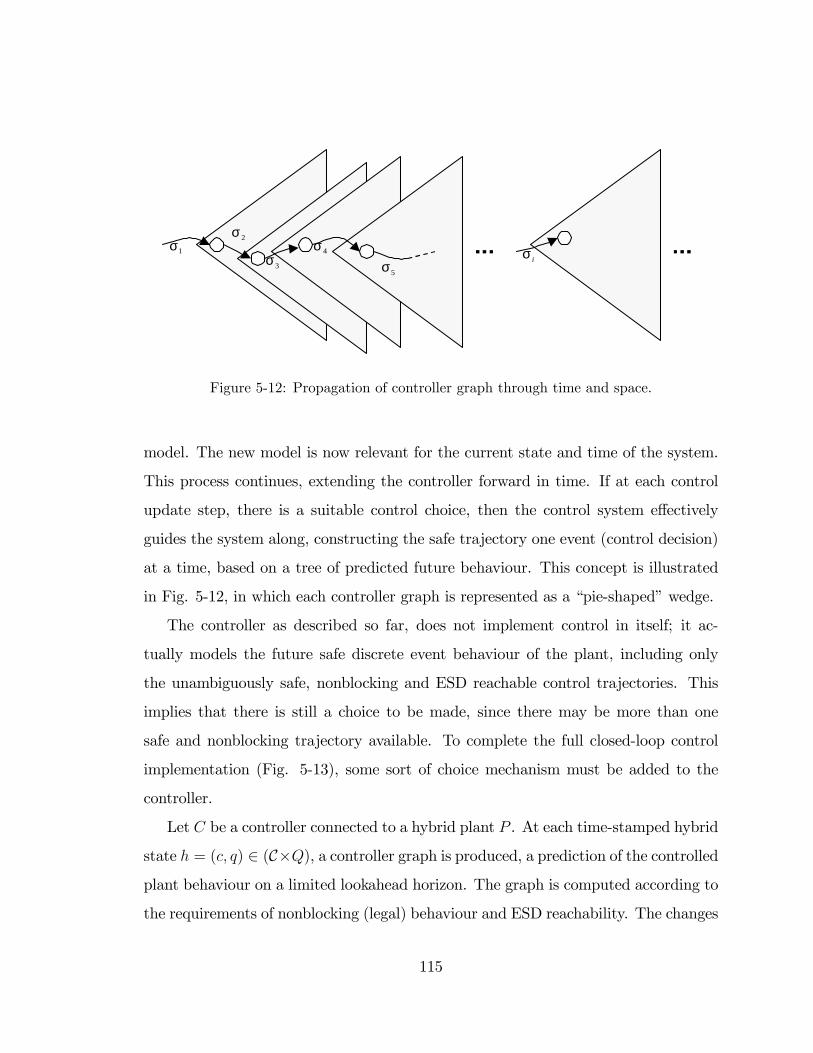
1σ2σ
3σ4σ
5σiσ
Figure 5-12: Propagation of controller graph through time and space.
model. The new model is now relevant for the current state and time of the system.
This process continues, extending the controller forward in time. If at each control
update step, there is a suitable control choice, then the control system e¤ectively
guides the system along, constructing the safe trajectory one event (control decision)
at a time, based on a tree of predicted future behaviour. This concept is illustrated
in Fig. 5-12, in which each controller graph is represented as a �pie-shaped�wedge.
The controller as described so far, does not implement control in itself; it ac-
tually models the future safe discrete event behaviour of the plant, including only
the unambiguously safe, nonblocking and ESD reachable control trajectories. This
implies that there is still a choice to be made, since there may be more than one
safe and nonblocking trajectory available. To complete the full closed-loop control
implementation (Fig. 5-13), some sort of choice mechanism must be added to the
controller.
Let C be a controller connected to a hybrid plant P . At each time-stamped hybrid
state h = (c; q) 2 (C�Q), a controller graph is produced, a prediction of the controlled
plant behaviour on a limited lookahead horizon. The graph is computed according to
the requirements of nonblocking (legal) behaviour and ESD reachability. The changes
115
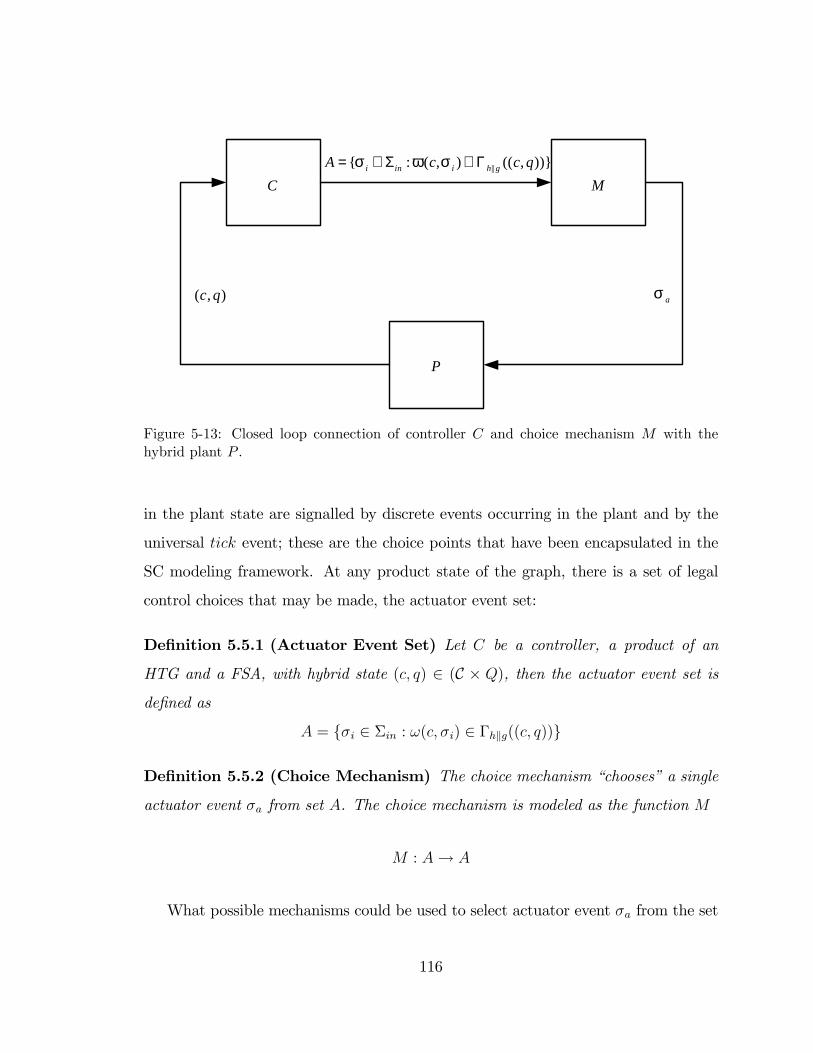
P
( , )c q
C||{ : ( , ) (( , ))}i in i h gA c c qσ ω σ= ∈ Σ ∈ Γ
M
aσ
Figure 5-13: Closed loop connection of controller C and choice mechanism M with thehybrid plant P .
in the plant state are signalled by discrete events occurring in the plant and by the
universal tick event; these are the choice points that have been encapsulated in the
SC modeling framework. At any product state of the graph, there is a set of legal
control choices that may be made, the actuator event set:
De�nition 5.5.1 (Actuator Event Set) Let C be a controller, a product of an
HTG and a FSA, with hybrid state (c; q) 2 (C � Q), then the actuator event set is
de�ned as
A = f�i 2 �in : !(c; �i) 2 �hkg((c; q))g
De�nition 5.5.2 (Choice Mechanism) The choice mechanism �chooses�a single
actuator event �a from set A. The choice mechanism is modeled as the function M
M : A! A
What possible mechanisms could be used to select actuator event �a from the set
116
of legal actuator events A? Choice mechanisms M; can be classi�ed as either manual
or automatic techniques. In the case of manual choice technique, a human operator
picks an actuator event �a 2 A using some heuristic to select �the best�action. This
is known as �human-in-the-loop�(HIL) control. Provided that A 6= ;; the operator�s
actions are guaranteed always to be safe, since the controller presents only actuator
events that lead to nonblocking and ESD-reachable states.
Although nonblocking and ESD states are essentially indistinguishable from each
other, the choice mechanism must discriminate between ESD reachable and �pure�
nonblocking choices, as in Table 5.1. Actuator events fall into two sets
A = Aen [ Ae
where Aen is the set of control events that lead to ESD reachable and nonblocking
trajectories, and the set Ae of events that lead only to an emergency shutdown. It
is preferable to choose actions that have some chance of continuing without invoking
an emergency shutdown.
Automatic control choice mechanisms, lacking human system knowledge on which
to base a choice of �a may operate in variety of ways including (but are not limited
to):
1. Minimum switching: minimize the number of times the actuator settings are
changed.
2. Optimal: Attempt to minimize some sort of cost/performance functional not
already captured in the speci�cation. Such a scheme might involve assigning
weighting factors to states in the plant model and assigning cost factors to
input (control) events for example. The control action considered to be optimal
by these rules would then be selected by M , which is essentially a dynamic
programming problem.
117
3. Stochastic: a choice mechanism based on probabilities of outcomes, a Markov
decision problem.
4. Other: Choose control action based on the number of states of the controller
subgraphs. A greater number of states may improve the likelihood of a non-
blocking continuation beyond the lookahead horizon.
As just indicated, there are many possible techniques to implement M , but they
will not be covered in any further detail. The behaviour of M does not a¤ect our
analysis, since all previous sections have been based on the assumption that some
event will be selected and the state of the plant will be advanced. Exactly how the
event is selected is not central to further discussion.
5.5.1 Online Operation: Controller Update Cycle
In any real-time control process, there are a set of scheduled actions that must be
repeatedly executed, usually at some regular time interval �t called the scan time.
For a control system, this set of actions will be called the control kernel, with the term
kernel used in the context of software engineering and not its mathematical meaning.
For the real-time process to proceed without failure, each of the scheduled actions
within the kernel must complete within a predictable and �nite time. Additionally,
the sum of these times must not exceed a �nite time interval �t. A digital control
system is such a real-time process, with one example being that of an industrial
programmable logic controller (PLC).
Example 5.5.1 (Digital Control (motor speed)) An example of a digital con-
troller is a DC motor speed control system. The actions to be executed in the control
kernel is as follows:
1. Measurement: sample motor speed
2. Compute control solution: Proportional, integral di¤erential control solution
118
3. Output control action: send control solution to ampli�er
Example 5.5.2 (Digital Control with State Estimation) An example of con-
trol and the comparison to optimal control with state estimation.
1. Output control action: send control solution to actuator
2. Measurement: sample feedback signal
3. State estimate: predict future value of system state
4. Compute control solution: using state estimate and controller gain matrix
With an online control scheme, the control kernel is executed repeatedly as the
system moves forward in (real) time. An outline of the scheduled actions within the
control kernel is, after initialization,
1. choose the control action (�a),
2. synchronize the controller (state/event synchronization)
3. recompute controller
The controller is computed for the �rst time, starting at the initial product state
of the plant and speci�cation models. If the controller exists for the initial condition
(initialization is successful), then the controller can be �enabled�or allowed to execute
physically in connection with the plant. Referring to Fig. 5-13, the choice mechanism
selects the event to apply to the plant from the subset of events that are enabled by
the controller A. At this point, the plant dynamics of the selected continuous system
model will begin the progression of the plant state towards the next choice point.
Immediately, the synthesis of a controller must be initiated, starting from the next
state which has been selected by the operator (the human in the loop) or by some
other process. This process continues as long as the controller is online and enabled.
119
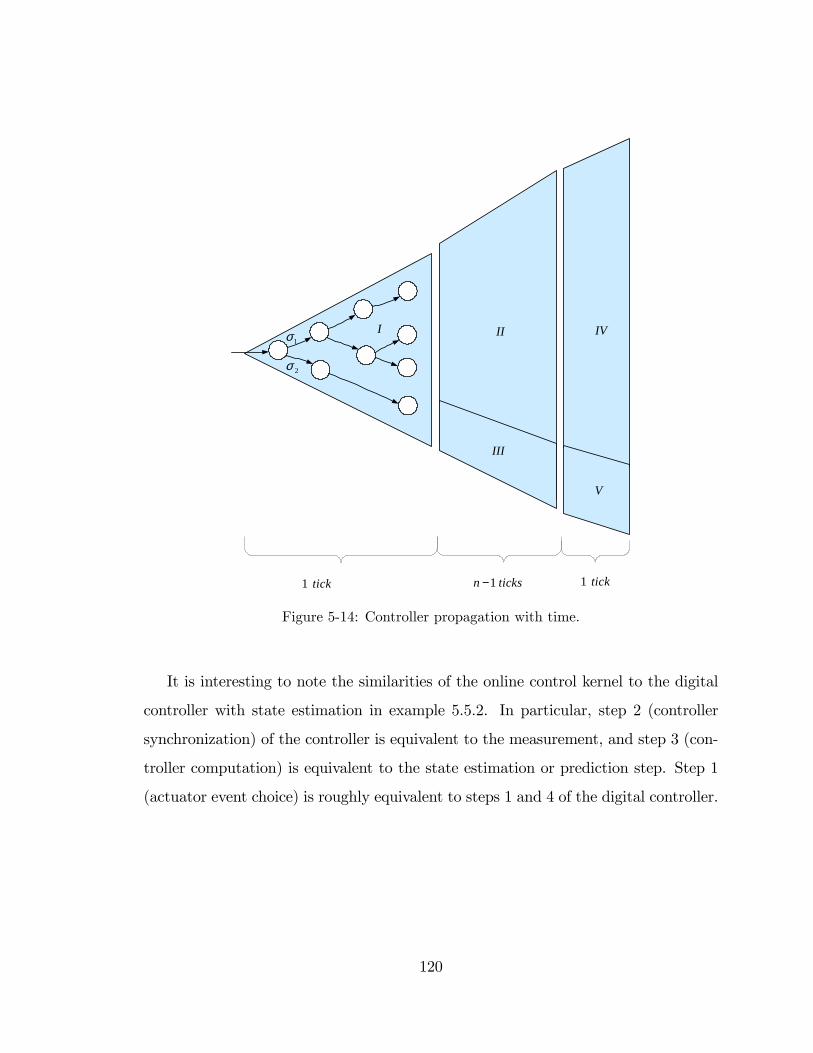
tick1 ticksn 1− tick1
2σ
1σI II IV
V
III
Figure 5-14: Controller propagation with time.
It is interesting to note the similarities of the online control kernel to the digital
controller with state estimation in example 5.5.2. In particular, step 2 (controller
synchronization) of the controller is equivalent to the measurement, and step 3 (con-
troller computation) is equivalent to the state estimation or prediction step. Step 1
(actuator event choice) is roughly equivalent to steps 1 and 4 of the digital controller.
120
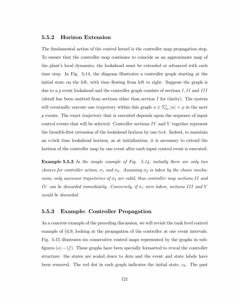
5.5.2 Horizon Extension
The fundamental action of the control kernel is the controller map propagation step.
To ensure that the controller map continues to coincide as an approximate map of
the plant�s local dynamics, the lookahead must be extended or advanced with each
time step. In Fig. 5-14, the diagram illustrates a controller graph starting at the
initial state on the left, with time �owing from left to right. Suppose the graph is
due to a p event lookahead and the controller graph consists of sections I; II and III
(detail has been omitted from sections other than section I for clarity). The system
will eventually execute one trajectory within this graph u 2 ��in; juj = p in the next
p events. The exact trajectory that is executed depends upon the sequence of input
control events that will be selected. Controller sections IV and V together represent
the breadth-�rst extension of the lookahead horizon by one tick. Indeed, to maintain
an n-tick time lookahead horizon, as at initialization, it is necessary to extend the
horizon of the controller map by one event after each input control event is executed.
Example 5.5.3 In the simple example of Fig. 5-14, initially there are only two
choices for controller action, �1 and �2. Assuming �2 is taken by the choice mecha-
nism, only successor trajectories of �2 are valid, thus controller map sections II and
IV can be discarded immediately. Conversely, if �1 were taken, sections III and V
would be discarded.
5.5.3 Example: Controller Propagation
As a concrete example of the preceding discussion, we will revisit the tank level control
example of §4.9, looking at the propagation of the controller at one event intervals.
Fig. 5-15 illustrates six consecutive control maps represented by the graphs in sub-
�gures (a)� (f). These graphs have been specially formatted to reveal the controller
structure: the states are scaled down to dots and the event and state labels have
been removed. The red dot in each graph indicates the initial state, c0. The past
121
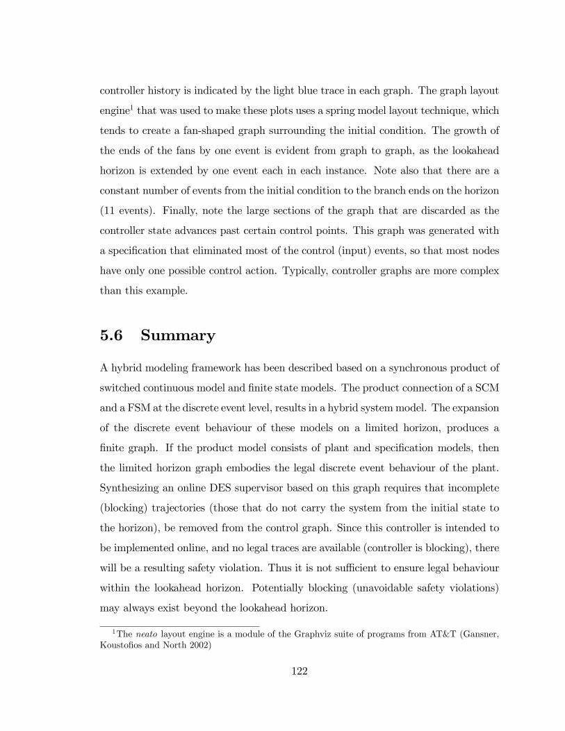
controller history is indicated by the light blue trace in each graph. The graph layout
engine1 that was used to make these plots uses a spring model layout technique, which
tends to create a fan-shaped graph surrounding the initial condition. The growth of
the ends of the fans by one event is evident from graph to graph, as the lookahead
horizon is extended by one event each in each instance. Note also that there are a
constant number of events from the initial condition to the branch ends on the horizon
(11 events). Finally, note the large sections of the graph that are discarded as the
controller state advances past certain control points. This graph was generated with
a speci�cation that eliminated most of the control (input) events, so that most nodes
have only one possible control action. Typically, controller graphs are more complex
than this example.
5.6 Summary
A hybrid modeling framework has been described based on a synchronous product of
switched continuous model and �nite state models. The product connection of a SCM
and a FSM at the discrete event level, results in a hybrid systemmodel. The expansion
of the discrete event behaviour of these models on a limited horizon, produces a
�nite graph. If the product model consists of plant and speci�cation models, then
the limited horizon graph embodies the legal discrete event behaviour of the plant.
Synthesizing an online DES supervisor based on this graph requires that incomplete
(blocking) trajectories (those that do not carry the system from the initial state to
the horizon), be removed from the control graph. Since this controller is intended to
be implemented online, and no legal traces are available (controller is blocking), there
will be a resulting safety violation. Thus it is not su¢ cient to ensure legal behaviour
within the lookahead horizon. Potentially blocking (unavoidable safety violations)
may always exist beyond the lookahead horizon.
1The neato layout engine is a module of the Graphviz suite of programs from AT&T (Gansner,Kousto�os and North 2002)
122
(a) (b)
(c) (d)
(e) (f)
Figure 5-15: Controller graph propagation through six events.
123
By establishing a special state called an emergency shutdown state, it is possible
to always guarantee the safety of our system. The so-called fail-safe controller always
requires that valid trajectories be ESD state reachable. This conservative control pol-
icy assumes that beyond the horizon, there will be a safety violation. Therefore, even
safe nonblocking trajectories will be eliminated because they cannot be guaranteed
to be safe beyond the horizon, the cost of the safety guarantee. Within the described
modeling framework, conditions for the existence of the fail-safe controller have been
established.
The controller is, by necessity an online controller, because of the need to reduce
complexity and to respond to time varying modeling conditions. Complexity reduc-
tion forces a limited lookahead horizon model; this model represents a �snapshot�
of the system state space. The controller designed for this snapshot must be moved
along in time and state as the controlled system (plant) progresses.
The next chapter will take the concepts of this and the previous chapters and
develop the implementation-speci�c details for the fail-safe online controller.
124
Chapter6Computation: From Theory to
Implementation
In the previous chapter, a framework was designed that enables an SCM model
to be synchronized with multiple FSM models in a discrete event fashion. The
resulting synchronized (product) model is a form of hybrid model since it has hybrid
states. This framework also makes it possible to synthesize supervisory discrete event
controllers for the modeled hybrid system. Control is exercised as a sequence of
discrete event control actions, applied by the controller at speci�ed system states
in dense-time. These control actions are planned by predicting the behaviour of
the modeled system on a limited lookahead horizon. Through the incorporation
of a specially marked state known as an emergency shutdown state, the controlled
system can be guaranteed to be safe (once the controller successfully initializes). The
controller model assumes that illegal states are just beyond the lookahead horizon.
This pessimistic outlook leads to controller conservatism: the controller requires that
at least one emergency shutdown trajectory must always be present in the control
structure.
This chapter details the general computational approach, the algorithmic imple-
mentation of the modeling concepts, and the speci�c implementation of a controller
125
synthesis and modeling software package.
6.1 Style
In the previous chapter, the theoretical considerations of the DES controller for a
hybrid system were outlined. This section will examine the basic computational
approach that has been adopted. There are three fundamental concepts that are nec-
essary to the control implementation, these are: lazy computing, limited lookahead,
and online implementation. These techniques will be leveraged to develop an e¢ cient
computational framework for modeling, controller synthesis, and control. Reduction
of computational complexity is of utmost importance to our controller implementa-
tion, since it is to be implemented as an online controller. First, we will examine the
concept of lazy computing,and its applicability to computing DES supervisors.
6.1.1 Lazy Computing Model
The term �lazy� is used here in the sense of expending the least e¤ort necessary to
accomplish a job. It is a technique that helps to reduce computational complexity
in space and time. Essentially, we are contrasting a hierarchical product model with
that of its �attened equivalent model. This hierarchical approach to �nite state mod-
eling has been exploited before to avoid the state explosion problem that occurs with
multiple product machines. In (Brave and Heymann 1991) a hierarchical statechart
approach is taken for modeling while (Gaudin and Marchand 2005) uses the hier-
archical approach to synthesize supervisors in systems without shared events. This
hierarchical technique lends itself well to the state-based techniques that are used
to construct the controller. In this section, a simple example in discrete event su-
pervisory control synthesis using the lazy technique will serve to illustrate the lazy
computing advantages over a �keen� computing approach. While the example is
somewhat simplistic, it is a useful exercise to motivate the succeeding sections. The
126
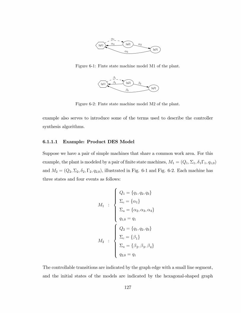
[q1][q2]
[q3]
α1
α2
α3
α4
[q1][q2]
[q3]
β1
β2
β3
β4
Figure 6-1: Finte state machine model M1 of the plant.
[q1][q2]
[q3]
α1
α2
α3
α4
[q1][q2]
[q3]
β1
β2
β3
β4
Figure 6-2: Finte state machine model M2 of the plant.
example also serves to introduce some of the terms used to describe the controller
synthesis algorithms.
6.1.1.1 Example: Product DES Model
Suppose we have a pair of simple machines that share a common work area. For this
example, the plant is modeled by a pair of �nite state machines,M1 = (Q1;�1; �1�1; q1;0)
andM2 = (Q2;�2; �2;�2; q2;0), illustrated in Fig. 6-1 and Fig. 6-2. Each machine has
three states and four events as follows:
M1 :
8>>>>>><>>>>>>:
Q1 = fq1; q2; q3g
�c = f�1g
�u = f�2; �3; �4g
q1;0 = q1
M2 :
8>>>>>><>>>>>>:
Q2 = fq1; q2; q3g
�c = f�1g
�u = f�2; �3; �4g
q2;0 = q1
The controllable transitions are indicated by the graph edge with a small line segment,
and the initial states of the models are indicated by the hexagonal-shaped graph
127
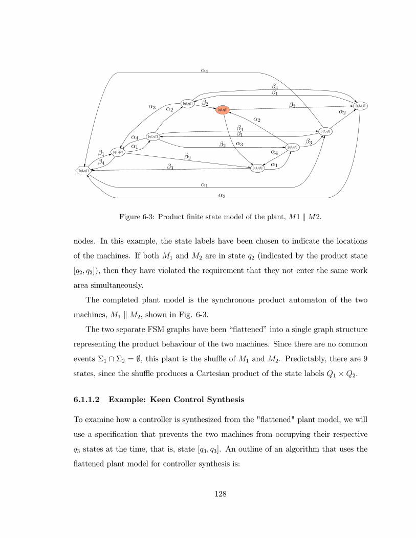
[q1,q1]
[q1,q2]
[q2,q1]
[q1,q3]
[q2,q2]
[q3,q1]
[q2,q3]
[q3,q2]
[q3,q3]
α1
α1
α1
α2
α2 α2
α3
α3
α3
α4
α4
α4
β1
β1
β1
β2
β2
β2
β3
β3
β3
β4
β4
β4
[q1,q1]
[q1,q2]
[q2,q1]
[q1,q3]
[q2,q2]
[q3,q1]
[q2,q3]
[q3,q2]
[q3,q3]
α1
α1
α1
α2
α2 α2
α3
α3
α3
α4
α4
α4
β1
β1
β1
β2
β2
β2
β3
β3
β3
β4
β4
β4
Figure 6-3: Product �nite state model of the plant, M1 kM2.
nodes. In this example, the state labels have been chosen to indicate the locations
of the machines. If both M1 and M2 are in state q2 (indicated by the product state
[q2; q2]), then they have violated the requirement that they not enter the same work
area simultaneously.
The completed plant model is the synchronous product automaton of the two
machines, M1 kM2, shown in Fig. 6-3.
The two separate FSM graphs have been ��attened�into a single graph structure
representing the product behaviour of the two machines. Since there are no common
events �1 \ �2 = ;, this plant is the shu e of M1 and M2. Predictably, there are 9
states, since the shu e produces a Cartesian product of the state labels Q1 �Q2.
6.1.1.2 Example: Keen Control Synthesis
To examine how a controller is synthesized from the "�attened" plant model, we will
use a speci�cation that prevents the two machines from occupying their respective
q3 states at the time, that is, state [q3; q3]. An outline of an algorithm that uses the
�attened plant model for controller synthesis is:
128
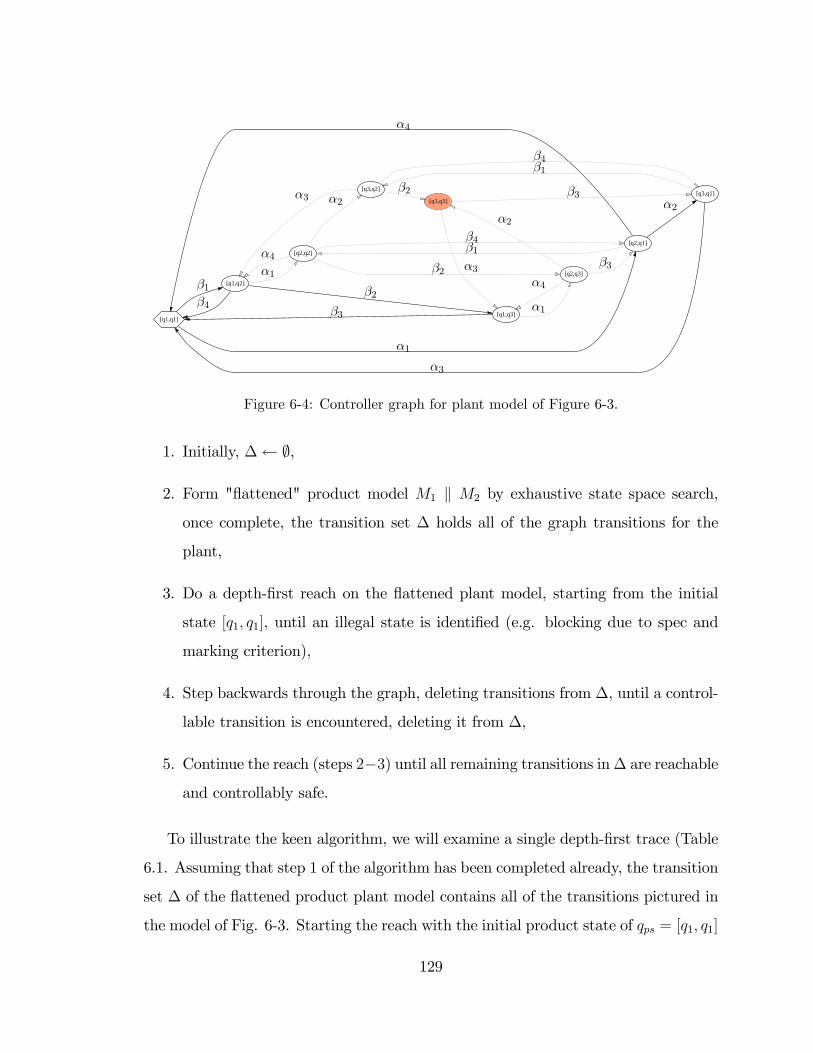
[q1,q1]
[q1,q2]
[q2,q1]
[q1,q3]
[q2,q2]
[q3,q1]
[q2,q3]
[q3,q2]
[q3,q3]
α1
α1
α1
α2
α2 α2
α3
α3
α3
α4
α4
α4
β1
β1
β1
β2
β2
β2
β3
β3
β3
β4
β4
β4
[q1,q1]
[q1,q2]
[q2,q1]
[q1,q3]
[q2,q2]
[q3,q1]
[q2,q3]
[q3,q2]
[q3,q3]
α1
α1
α1
α2
α2 α2
α3
α3
α3
α4
α4
α4
β1
β1
β1
β2
β2
β2
β3
β3
β3
β4
β4
β4
Figure 6-4: Controller graph for plant model of Figure 6-3.
1. Initially, � ;,
2. Form "�attened" product model M1 k M2 by exhaustive state space search,
once complete, the transition set � holds all of the graph transitions for the
plant,
3. Do a depth-�rst reach on the �attened plant model, starting from the initial
state [q1; q1], until an illegal state is identi�ed (e.g. blocking due to spec and
marking criterion),
4. Step backwards through the graph, deleting transitions from �, until a control-
lable transition is encountered, deleting it from �,
5. Continue the reach (steps 2�3) until all remaining transitions in� are reachable
and controllably safe.
To illustrate the keen algorithm, we will examine a single depth-�rst trace (Table
6.1. Assuming that step 1 of the algorithm has been completed already, the transition
set � of the �attened product plant model contains all of the transitions pictured in
the model of Fig. 6-3. Starting the reach with the initial product state of qps = [q1; q1]
129
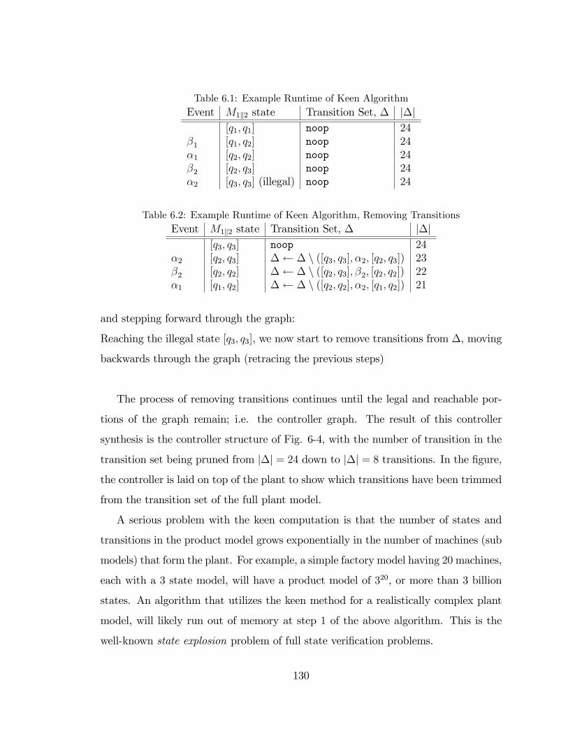
Table 6.1: Example Runtime of Keen AlgorithmEvent M1k2 state Transition Set, � j�j
[q1; q1] noop 24�1 [q1; q2] noop 24�1 [q2; q2] noop 24�2 [q2; q3] noop 24�2 [q3; q3] (illegal) noop 24
Table 6.2: Example Runtime of Keen Algorithm, Removing TransitionsEvent M1k2 state Transition Set, � j�j
[q3; q3] noop 24�2 [q2; q3] � � n ([q3; q3]; �2; [q2; q3]) 23�2 [q2; q2] � � n ([q2; q3]; �2; [q2; q2]) 22�1 [q1; q2] � � n ([q2; q2]; �2; [q1; q2]) 21
and stepping forward through the graph:
Reaching the illegal state [q3; q3], we now start to remove transitions from �, moving
backwards through the graph (retracing the previous steps)
The process of removing transitions continues until the legal and reachable por-
tions of the graph remain; i.e. the controller graph. The result of this controller
synthesis is the controller structure of Fig. 6-4, with the number of transition in the
transition set being pruned from j�j = 24 down to j�j = 8 transitions. In the �gure,
the controller is laid on top of the plant to show which transitions have been trimmed
from the transition set of the full plant model.
A serious problem with the keen computation is that the number of states and
transitions in the product model grows exponentially in the number of machines (sub
models) that form the plant. For example, a simple factory model having 20machines,
each with a 3 state model, will have a product model of 320, or more than 3 billion
states. An algorithm that utilizes the keen method for a realistically complex plant
model, will likely run out of memory at step 1 of the above algorithm. This is the
well-known state explosion problem of full state veri�cation problems.
130
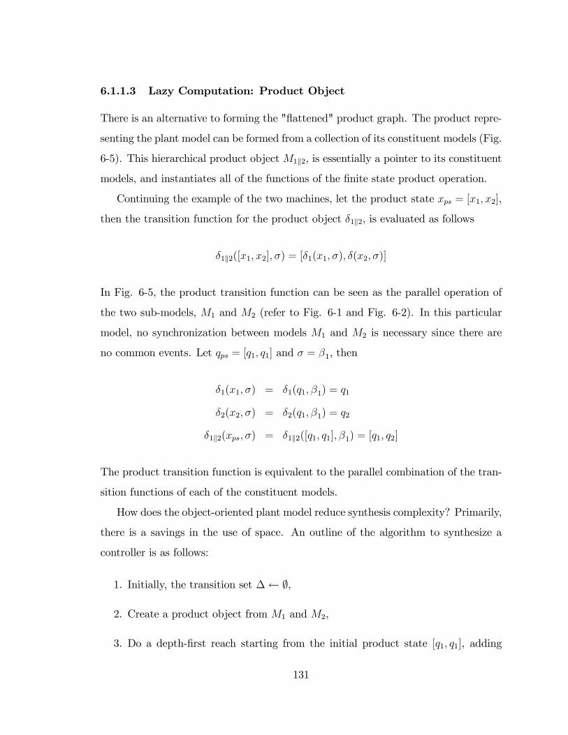
6.1.1.3 Lazy Computation: Product Object
There is an alternative to forming the "�attened" product graph. The product repre-
senting the plant model can be formed from a collection of its constituent models (Fig.
6-5). This hierarchical product object M1k2, is essentially a pointer to its constituent
models, and instantiates all of the functions of the �nite state product operation.
Continuing the example of the two machines, let the product state xps = [x1; x2],
then the transition function for the product object �1k2, is evaluated as follows
�1k2([x1; x2]; �) = [�1(x1; �); �(x2; �)]
In Fig. 6-5, the product transition function can be seen as the parallel operation of
the two sub-models, M1 and M2 (refer to Fig. 6-1 and Fig. 6-2). In this particular
model, no synchronization between models M1 and M2 is necessary since there are
no common events. Let qps = [q1; q1] and � = �1, then
�1(x1; �) = �1(q1; �1) = q1
�2(x2; �) = �2(q1; �1) = q2
�1k2(xps; �) = �1k2([q1; q1]; �1) = [q1; q2]
The product transition function is equivalent to the parallel combination of the tran-
sition functions of each of the constituent models.
How does the object-oriented plant model reduce synthesis complexity? Primarily,
there is a savings in the use of space. An outline of the algorithm to synthesize a
controller is as follows:
1. Initially, the transition set � ;,
2. Create a product object from M1 and M2,
3. Do a depth-�rst reach starting from the initial product state [q1; q1], adding
131
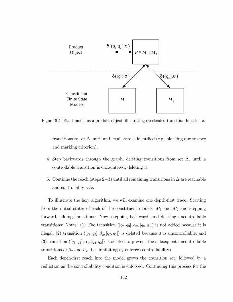
1 2(( , ), )q qδ σ
1M
1 2||P M M=
2M
1(( ), )qδ σ 2(( ), )qδ σ
ConstituentFinite State
Models
ProductObject
Figure 6-5: Plant model as a product object, illustrating overloaded transition function �.
transitions to set �, until an illegal state is identi�ed (e.g. blocking due to spec
and marking criterion),
4. Step backwards through the graph, deleting transitions from set �, until a
controllable transition is encountered, deleting it,
5. Continue the reach (steps 2�3) until all remaining transitions in� are reachable
and controllably safe.
To illustrate the lazy algorithm, we will examine one depth-�rst trace. Starting
from the initial states of each of the constituent models, M1 and M2 and stepping
forward, adding transitions: Now, stepping backward, and deleting uncontrollable
transitions: Notes: (1) The transition ([q2; q3]; �2; [q3; q3]) is not added because it is
illegal, (2) transition ([q2; q2]; �2; [q2; q3]) is deleted because it is uncontrollable, and
(3) transition ([q1; q2]; �1; [q2; q2]) is deleted to prevent the subsequent uncontrollable
transitions of �2 and �2 (i.e. inhibiting �1 enforces controllability).
Each depth-�rst reach into the model grows the transition set, followed by a
reduction as the controllability condition is enforced. Continuing this process for the
132
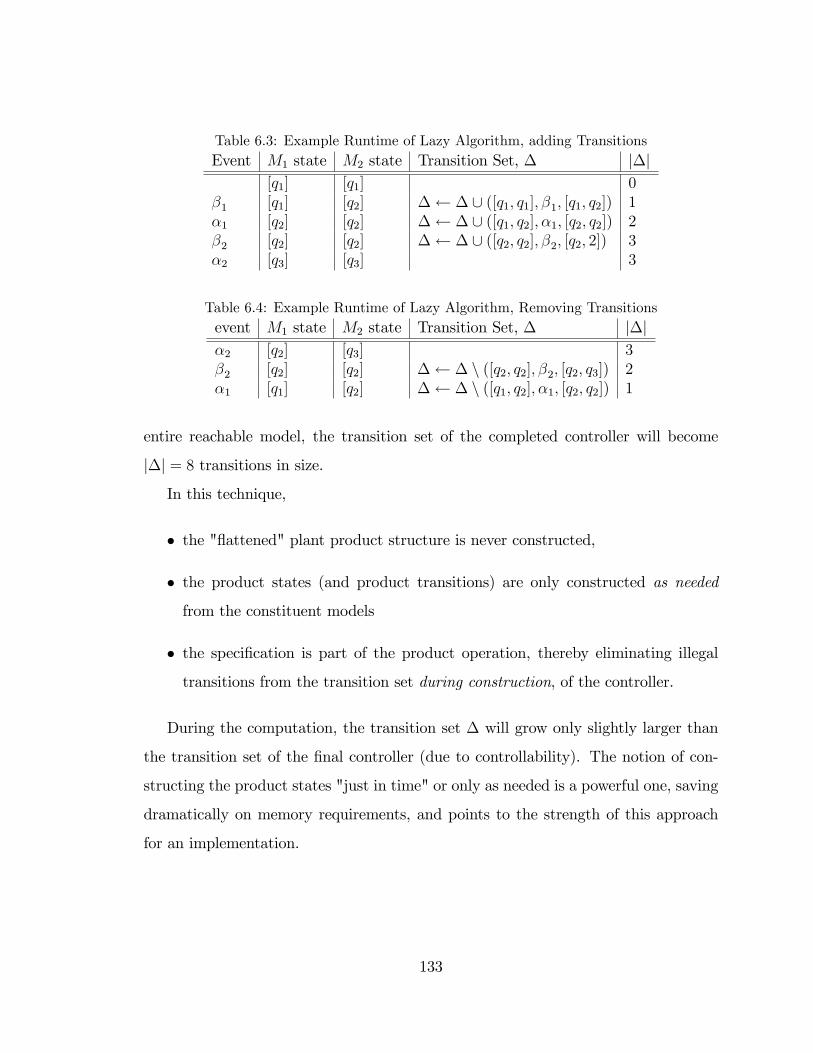
Table 6.3: Example Runtime of Lazy Algorithm, adding TransitionsEvent M1 state M2 state Transition Set, � j�j
[q1] [q1] 0�1 [q1] [q2] � � [ ([q1; q1]; �1; [q1; q2]) 1�1 [q2] [q2] � � [ ([q1; q2]; �1; [q2; q2]) 2�2 [q2] [q2] � � [ ([q2; q2]; �2; [q2; 2]) 3�2 [q3] [q3] 3
Table 6.4: Example Runtime of Lazy Algorithm, Removing Transitionsevent M1 state M2 state Transition Set, � j�j�2 [q2] [q3] 3�2 [q2] [q2] � � n ([q2; q2]; �2; [q2; q3]) 2�1 [q1] [q2] � � n ([q1; q2]; �1; [q2; q2]) 1
entire reachable model, the transition set of the completed controller will become
j�j = 8 transitions in size.
In this technique,
� the "�attened" plant product structure is never constructed,
� the product states (and product transitions) are only constructed as needed
from the constituent models
� the speci�cation is part of the product operation, thereby eliminating illegal
transitions from the transition set during construction, of the controller.
During the computation, the transition set � will grow only slightly larger than
the transition set of the �nal controller (due to controllability). The notion of con-
structing the product states "just in time" or only as needed is a powerful one, saving
dramatically on memory requirements, and points to the strength of this approach
for an implementation.
133
6.1.1.4 Example: Keen, Lazy Techniques
To contrast the two techniques, the keen method is a pruning process, while the lazy
method is an additive process. In the lazy technique, the plant and speci�cation are
represented by a product object model, that allows the product to be computed in a
"just in time" fashion. The product requires event synchronization between the mod-
els making up the product object. Providing there are some common events between
speci�cation and the plant models, the product will always have fewer transitions
than the �attened plant model alone. This leads to a reduction in space complexity
over the keen technique.
Example 6.1.1 This example uses the analogy of navigating across a portion of a
city (Fig. 6-6, (1)). The task of constructing a route that leads from the starting point
(the green triangle) to a desired destination (the red octagon) is akin to computing
a discrete event controller, with events corresponding to actions of left turn, right
turn, or go straight; the states (or control points) correspond to the intersections of
roads. Suppose the speci�cation (a rule) is that directions that take us further from
the destination (for example, in a euclidean sense) are illegal.Referring to Fig. 6-
6, the keen algorithm begins at (1) with no knowledge of the map, but exhaustively
builds a complete map (2); by traversing all of the routes that reach the destination,
building an exhaustive set of possible routes. Next, it checks each of these depth-�rst
routes against the speci�cation (the dotted contour lines indicate equal distance from
the destination), removing transitions that are illegal, until only legal routes remain,
as in (3). With the lazy technique, we start with an empty transition set (map) at (1).
Routes are gradually added to the map by testing each route against the speci�cation,
until the entire legal and reachable map has been constructed in (3). The result is that
the lazy algorithm achieves an identical result to the keen technique, with a single step
and with reduced space complexity. This is possible because the speci�cation is used
at design time, allowing illegal traces in many cases, to be eliminated before they are
134

Keen
KeenLazy
)1( )2(
)3(
Figure 6-6: Map navigation analogy for controller synthesis algorithms.
135
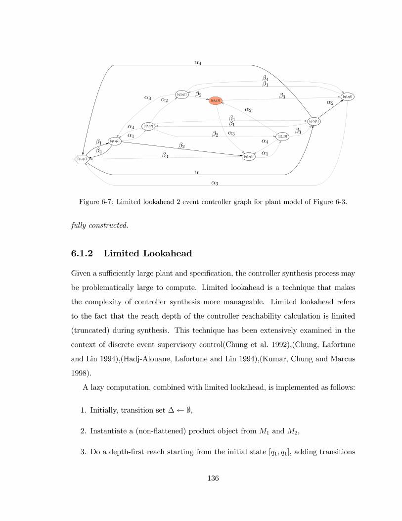
[q1,q1]
[q1,q2]
[q2,q1]
[q1,q3]
[q2,q2]
[q3,q1]
[q2,q3]
[q3,q2]
[q3,q3]
α1
α1
α1
α2
α2 α2
α3
α3
α3
α4
α4
α4
β1
β1
β1
β2
β2
β2
β3
β3
β3
β4
β4
β4
Figure 6-7: Limited lookahead 2 event controller graph for plant model of Figure 6-3.
fully constructed.
6.1.2 Limited Lookahead
Given a su¢ ciently large plant and speci�cation, the controller synthesis process may
be problematically large to compute. Limited lookahead is a technique that makes
the complexity of controller synthesis more manageable. Limited lookahead refers
to the fact that the reach depth of the controller reachability calculation is limited
(truncated) during synthesis. This technique has been extensively examined in the
context of discrete event supervisory control(Chung et al. 1992),(Chung, Lafortune
and Lin 1994),(Hadj-Alouane, Lafortune and Lin 1994),(Kumar, Chung and Marcus
1998).
A lazy computation, combined with limited lookahead, is implemented as follows:
1. Initially, transition set � ;,
2. Instantiate a (non-�attened) product object from M1 and M2,
3. Do a depth-�rst reach starting from the initial state [q1; q1], adding transitions
136
to set �, until either: (a) an illegal state is identi�ed (e.g. blocking due to spec
and marking criterion), or (b) the limited lookahead reach depth is reached,
4. Step backwards through the graph, deleting transitions from set �, until a
controllable transition is encountered, deleting it,
5. Continue the reach (steps 2� 3) until all remaining transitions in � are reach-
able, less than the reach depth and controllably safe.
While limited lookahead is e¤ective as a technique for complexity reduction, it is
not possible to guarantee safety and non-blocking behaviour since the controller is
designed for a partial model. Fig. 6-7 is the limited lookahead controller for the plant
of Fig. 6-3 with a 2-event lookahead. This technique can be applied to either the keen
or lazy techniques to provide a further reduction in space complexity. An additional
bene�t of the limited lookahead computation is that the space complexity is bounded.
Since the size of the computation is known ahead of time, the computational resources
can be planned making it more amenable to an online (real time) computation.
6.1.3 Online Computation
The terms online and o ine refer to the synthesis of the controller: o ine means the
controller is completely synthesized before the execution of the control, while online
control implies that the controller is synthesized during controller execution. Why
include the controller synthesis as part of the runtime system? Online controller syn-
thesis is a necessity to a limited lookahead control scheme. The controller map must
be extended to match the moving system state by advancing the lookahead horizon.
Moreover, the controller propagation process described in §5.5, allows us to deal with
a time-varying model or speci�cation. Online controller synthesis potentially allows
the controller to react to modeled, but unexpected disturbances, that a controller
constructed o ine cannot. A requirement of online controller synthesis is that the
137
controller must be synthesized repeatedly in a real-time environment. Thus, the com-
plexity of the controller synthesis computation must be of a predictable size, which,
in turn, is why a limited lookahead scheme is amenable to online implementation.
6.2 Software
A software package has been designed that implements the modeling and controller
synthesis framework described in the preceding sections. The package is calledHySynth,
for Hybrid Synthesis and is designed for the MatlabR environment. The software can
be used to develop system models with a mixture of switched continuous and �-
nite state models that represent the plant and speci�cation of the target system.
These models may be synchronized in a hierarchical product structure and then algo-
rithmically manipulated to synthesize discrete event supervisors. Functions are also
available to propagate the controllers and to simulate the controlled system. Addi-
tional functions are supplied to produce �nite state graph outputs of the models in a
variety of formats, including Postscript, Portable Document Format (PDF) and Vir-
tual Reality Modeling Language (VRML). These outputs give the designer a means
of visualizing the individual constituent models and the larger product graphs for
troubleshooting purposes.
6.2.1 Architecture
HySynth exploits object-oriented programming (OOP) strategies. Models are stored
as instantiations of appropriate classes:
fsm Class for deterministic �nite state models, G = (Q;�; �;�; q0)
scm Class for switched continuous models, G = (F ;�; s0)
product Class for products of discrete event process objects, P
138
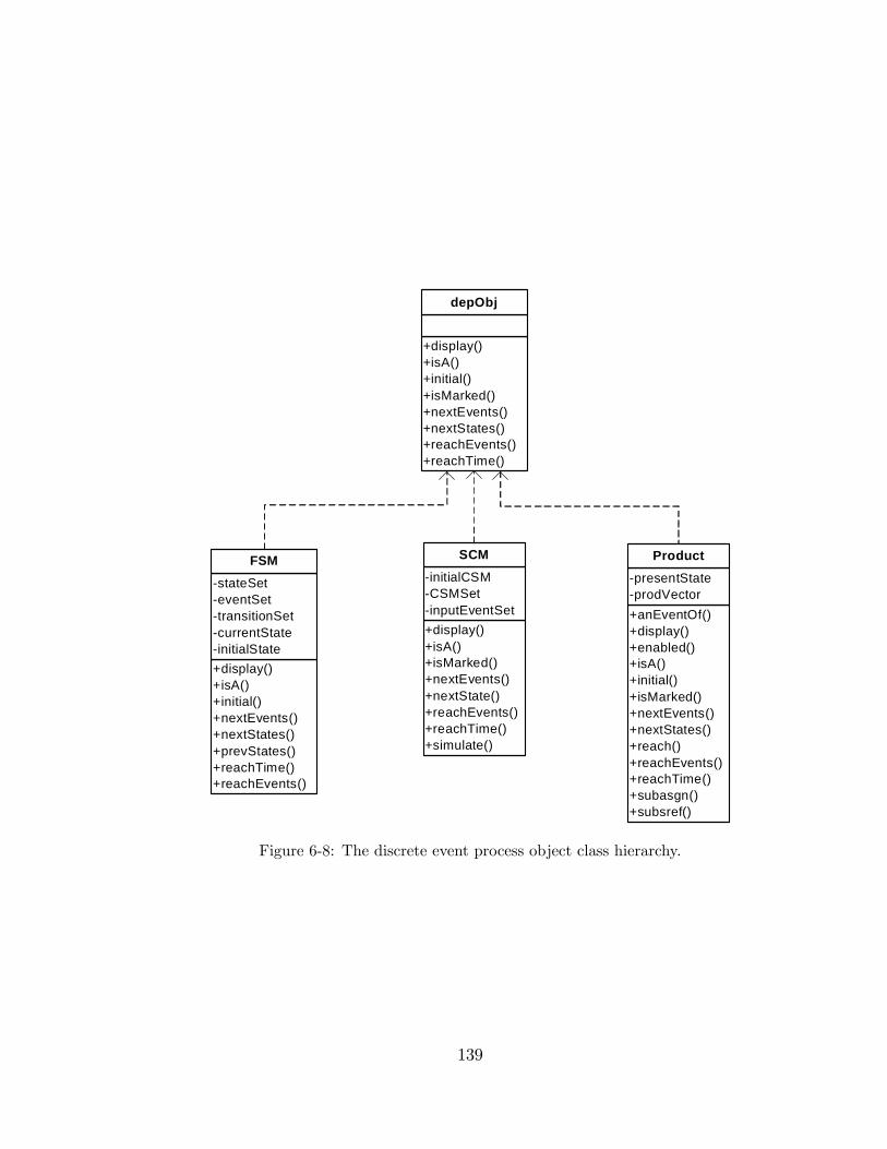
+display()+isA()+initial()+isMarked()+nextEvents()+nextStates()+reachEvents()+reachTime()
depObj
+display()+isA()+initial()+nextEvents()+nextStates()+prevStates()+reachTime()+reachEvents()
stateSeteventSettransitionSetcurrentStateinitialState
FSM
+display()+isA()+isMarked()+nextEvents()+nextState()+reachEvents()+reachTime()+simulate()
initialCSMCSMSetinputEventSet
SCM
+anEventOf()+display()+enabled()+isA()+initial()+isMarked()+nextEvents()+nextStates()+reach()+reachEvents()+reachTime()+subasgn()+subsref()
presentStateprodVector
Product
Figure 6-8: The discrete event process object class hierarchy.
139
Each of these classes is derived from an abstract base class, the discrete event
process object class, or depobj class (Fig. 6-8). The product class acts as a hetero-
geneous container that stores a vector of depobj objects; i.e. types fsm, scm and
also product. This recursive containment ability (a product may contain another
product) permits hierarchical models to be constructed. The three classes present a
common interface, implementing a variety of polymorphic methods. These methods
permit the hierarchical models to be manipulated for analysis, simulation and control
synthesis.
An example of a polymorphic function is the nextEvents(state) method that
returns the set of next events for an object, given an argument of state. For a deter-
ministic �nite state machine G = (Q;�; �;�; q0), the state argument is a �nite state,
and the function evaluates the enabled events function �, returning a set of discrete
events. For a switched continuous model G = (F ;�; s0), the function conducts a sim-
ulation for each s 2 F , with the state argument, a time-stamped continuous state.
Simulation trajectories that cross the state boundaries (as de�ned by the respective
set of partitioning functionals) generate events that become elements of the set of
next events. This function equates to the enabled events function �h of the HTG.
This discussion points out the need for a variety of types of states, since the
domain of each function varies:
finiteState Class for �nite state models, q 2 Q
ctsState Class for continuous state variables, x 2 Rn
pState Class for product states, ps.
The domain of the product state has been deliberately omitted, to allow for a
containment. These classes are derived from an abstract base class, the stateObject
class (Fig. 6-9). As with the product class, the pState class is a heterogenous con-
tainer, that stores a vector of stateObject objects. And like the product class, it can
140

+ctsState()+display()+isA()+isMarked()+stateLabel()
timeStampstateVector
ctsState
+display()+eq()+finiteState()+isA()+isMarked()+stateLabel()
statemarking
finiteState
+display()+isA()+isEqual()+isMarked()+pstate()+stateLabel()+subasgn()+subsref()
pStateVector
pState
+display()+isA()+isMarked()
stateObject
Figure 6-9: State object class hierarchy.
recursively store other pstate objects, allowing for states to match the hierarchical
structure of the models.
The state space of a product object is not generated until run time, since the
hierarchical object structure is maintained. By generating the state space only as
needed using the lazy computation model, the costly computation of the ��attened�
product state space is avoided. Fig. 6-10 illustrates a model constructed using the
product class.
All of the algorithms that implement HySynth functions have been written to
exploit this hierarchical storage of models. The core classes of HySynth in Fig.
6-8 and Fig. 6-9 have been implemented in Matlab scripting language, using the
OOP programming features of Matlab (MATLAB Programming 2006). The resulting
modeling framework essentially extends Matlab�s interpretive command set to allow
for modeling, analysis, controller synthesis and visualization.
141
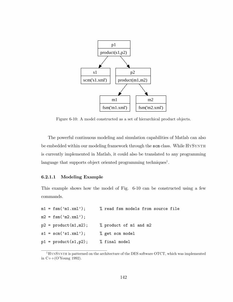
p1
product(s1,p2)
s1
scm('s1.xml')
p2
product(m1,m2)
m1
fsm('m1.xml')
m2
fsm('m2.xml')
Figure 6-10: A model constructed as a set of hierarchical product objects.
The powerful continuous modeling and simulation capabilities of Matlab can also
be embedded within our modeling framework through the scm class. WhileHySynth
is currently implemented in Matlab, it could also be translated to any programming
language that supports object oriented programming techniques1.
6.2.1.1 Modeling Example
This example shows how the model of Fig. 6-10 can be constructed using a few
commands.
m1 = fsm(�m1.xml�); % read fsm models from source file
m2 = fsm(�m2.xml�);
p2 = product(m1,m2); % product of m1 and m2
s1 = scm(�s1.xml�); % get scm model
p1 = product(s1,p2); % final model
1HynSynth is patterned on the architecture of the DES software OTCT, which was implementedin C++(O�Young 1992).
142
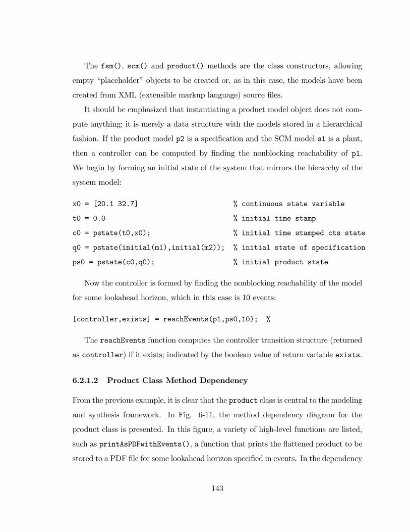
The fsm(), scm() and product() methods are the class constructors, allowing
empty �placeholder�objects to be created or, as in this case, the models have been
created from XML (extensible markup language) source �les.
It should be emphasized that instantiating a product model object does not com-
pute anything; it is merely a data structure with the models stored in a hierarchical
fashion. If the product model p2 is a speci�cation and the SCM model s1 is a plant,
then a controller can be computed by �nding the nonblocking reachability of p1.
We begin by forming an initial state of the system that mirrors the hierarchy of the
system model:
x0 = [20.1 32.7] % continuous state variable
t0 = 0.0 % initial time stamp
c0 = pstate(t0,x0); % initial time stamped cts state
q0 = pstate(initial(m1),initial(m2)); % initial state of specification
ps0 = pstate(c0,q0); % initial product state
Now the controller is formed by �nding the nonblocking reachability of the model
for some lookahead horizon, which in this case is 10 events:
[controller,exists] = reachEvents(p1,ps0,10); %
The reachEvents function computes the controller transition structure (returned
as controller) if it exists; indicated by the boolean value of return variable exists.
6.2.1.2 Product Class Method Dependency
From the previous example, it is clear that the product class is central to the modeling
and synthesis framework. In Fig. 6-11, the method dependency diagram for the
product class is presented. In this �gure, a variety of high-level functions are listed,
such as printAsPDFwithEvents(), a function that prints the �attened product to be
stored to a PDF �le for some lookahead horizon speci�ed in events. In the dependency
143
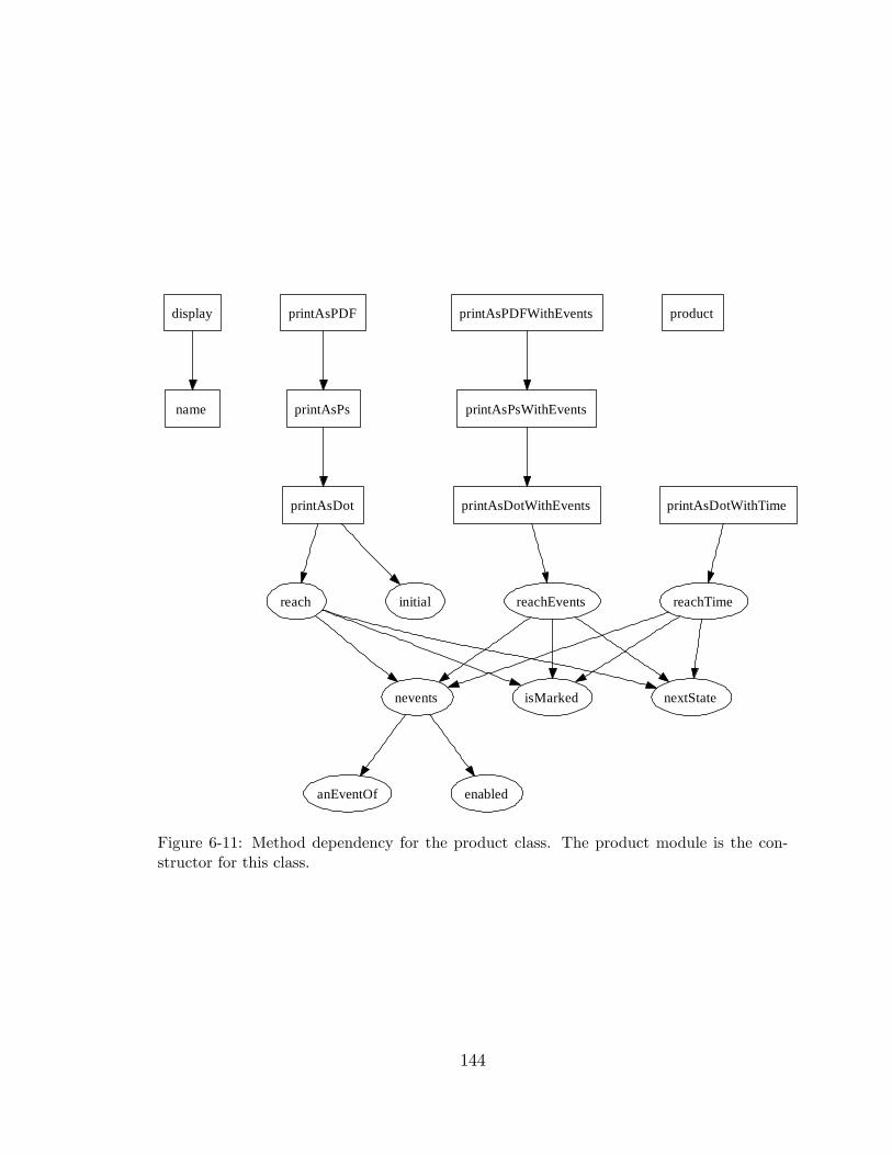
display
name
nevents
anEventOf enabled
printAsDot
initialreach
isMarked nextState
printAsDotWithEvents
reachEvents
printAsDotWithTime
reachTime
printAsPDF
printAsPs
printAsPDFWithEvents
printAsPsWithEvents
product
Figure 6-11: Method dependency for the product class. The product module is the con-structor for this class.
144
Figure 6-12: Main menu of JFLAP automata and formal languages package.
diagram, recursive functions are indicated as ellipses. The recursion is necessary for
the hierarchical storage of the product class.
6.2.2 User Interface
The user interface for HySynth was developed for prototyping purposes, but is
reasonably easy to use. A simple graphical user interface is provided by a third-party
software package, call JFLAP(Rodger and Finley 2006). This package is intended
to be used as a tool for teaching students automata and formal languages, but for
HySynth, it serves as a front-end for �nite state machine capture. From the main
menu (Fig. 6-12), the user selects the Finite Automaton option, which brings up an
empty �nite automaton capture window. In Fig. 6-13, the capture window has an
automaton entered already. Once the designer has completed the design, the FSA
may be stored to disk in an XML format �le with default extension of .j¤. The �nite
state model object in HySynth has a method that enables it to parse this �le from
disk, creating an fsm object.
The graph visualization capability of HySynth is based on the AT&T Graphviz
graph layout engine (Gansner et al. 2002). Smaller graphs (<100 states) are useful to
145
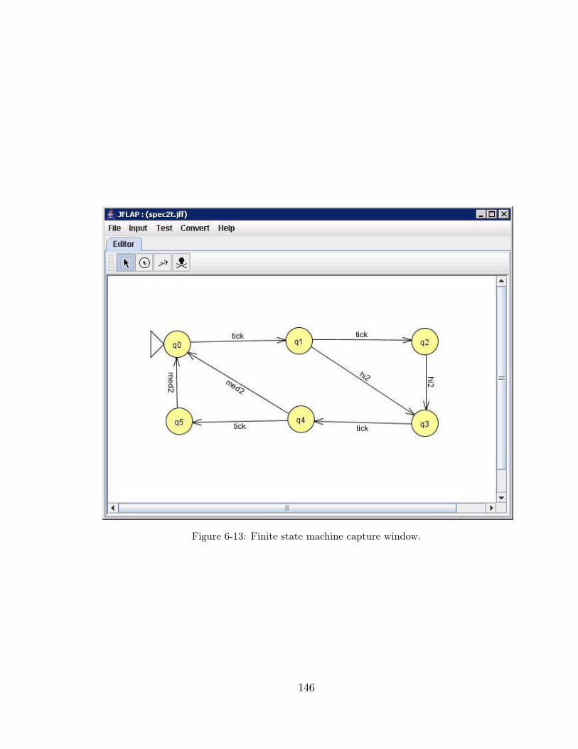
Figure 6-13: Finite state machine capture window.
146
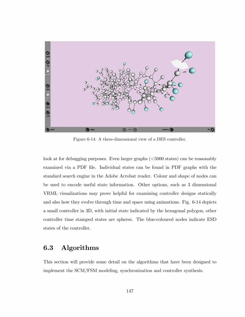
Figure 6-14: A three-dimensional view of a DES controller.
look at for debugging purposes. Even larger graphs (<5000 states) can be reasonably
examined via a PDF �le. Individual states can be found in PDF graphs with the
standard search engine in the Adobe Acrobat reader. Colour and shape of nodes can
be used to encode useful state information. Other options, such as 3 dimensional
VRML visualizations may prove helpful for examining controller designs statically
and also how they evolve through time and space using animations. Fig. 6-14 depicts
a small controller in 3D, with initial state indicated by the hexagonal polygon, other
controller time stamped states are spheres. The blue-coloured nodes indicate ESD
states of the controller.
6.3 Algorithms
This section will provide some detail on the algorithms that have been designed to
implement the SCM/FSM modeling, synchronization and controller synthesis.
147
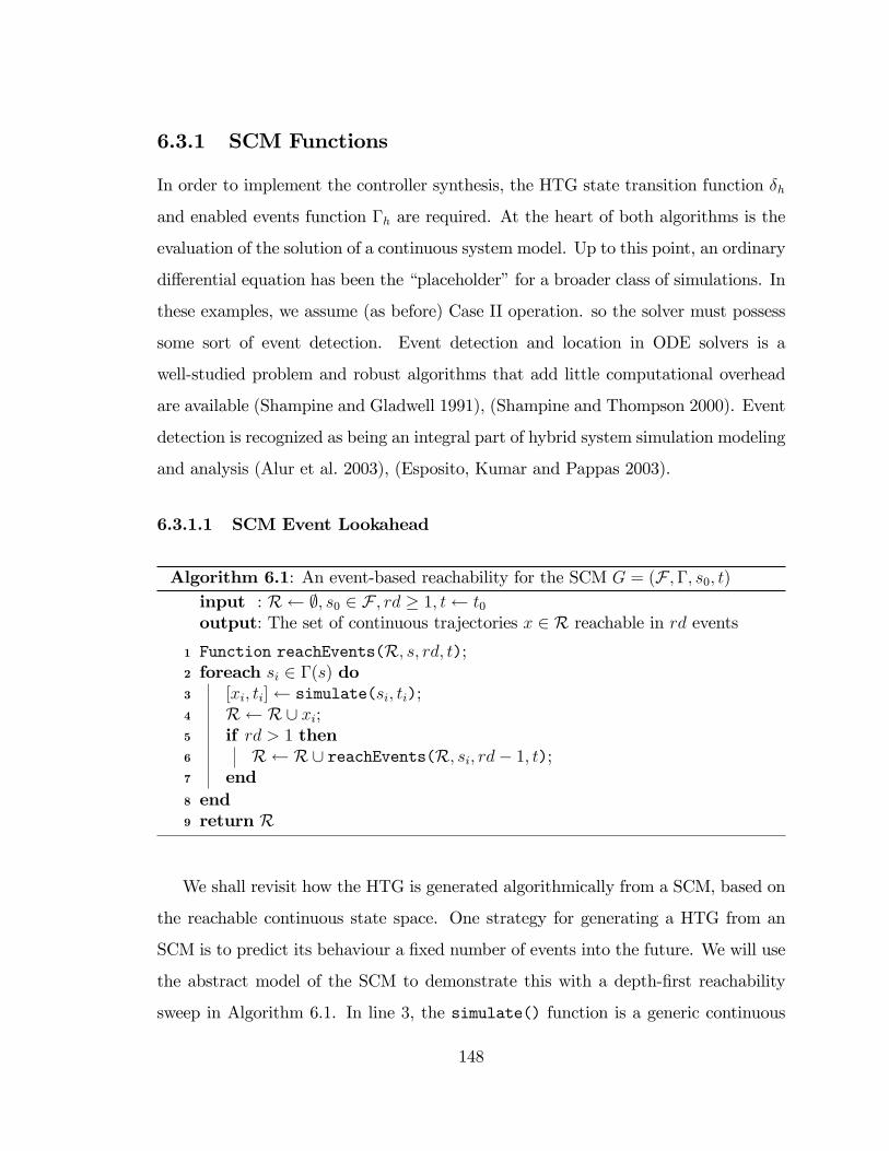
6.3.1 SCM Functions
In order to implement the controller synthesis, the HTG state transition function �h
and enabled events function �h are required. At the heart of both algorithms is the
evaluation of the solution of a continuous system model. Up to this point, an ordinary
di¤erential equation has been the �placeholder�for a broader class of simulations. In
these examples, we assume (as before) Case II operation. so the solver must possess
some sort of event detection. Event detection and location in ODE solvers is a
well-studied problem and robust algorithms that add little computational overhead
are available (Shampine and Gladwell 1991), (Shampine and Thompson 2000). Event
detection is recognized as being an integral part of hybrid system simulation modeling
and analysis (Alur et al. 2003), (Esposito, Kumar and Pappas 2003).
6.3.1.1 SCM Event Lookahead
Algorithm 6.1: An event-based reachability for the SCM G = (F ;�; s0; t)input : R ;; s0 2 F ; rd � 1; t t0output: The set of continuous trajectories x 2 R reachable in rd eventsFunction reachEvents(R; s; rd; t);1
foreach si 2 �(s) do2
[xi; ti] simulate(si; ti);3
R R[ xi;4
if rd > 1 then5
R R[ reachEvents(R; si; rd� 1; t);6
end7
end8
return R9
We shall revisit how the HTG is generated algorithmically from a SCM, based on
the reachable continuous state space. One strategy for generating a HTG from an
SCM is to predict its behaviour a �xed number of events into the future. We will use
the abstract model of the SCM to demonstrate this with a depth-�rst reachability
sweep in Algorithm 6.1. In line 3, the simulate() function is a generic continuous
148
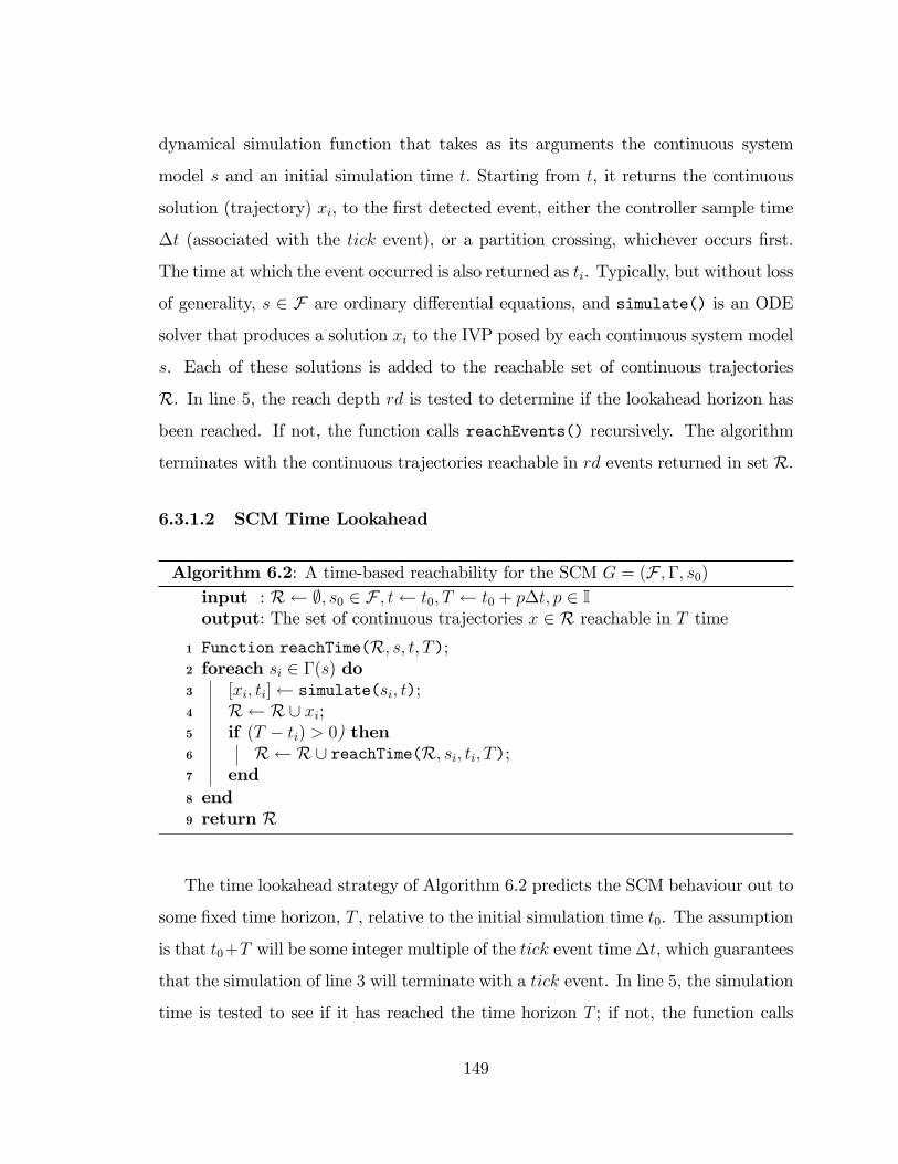
dynamical simulation function that takes as its arguments the continuous system
model s and an initial simulation time t: Starting from t, it returns the continuous
solution (trajectory) xi, to the �rst detected event, either the controller sample time
�t (associated with the tick event), or a partition crossing, whichever occurs �rst.
The time at which the event occurred is also returned as ti. Typically, but without loss
of generality, s 2 F are ordinary di¤erential equations, and simulate() is an ODE
solver that produces a solution xi to the IVP posed by each continuous system model
s. Each of these solutions is added to the reachable set of continuous trajectories
R. In line 5, the reach depth rd is tested to determine if the lookahead horizon has
been reached. If not, the function calls reachEvents() recursively. The algorithm
terminates with the continuous trajectories reachable in rd events returned in set R.
6.3.1.2 SCM Time Lookahead
Algorithm 6.2: A time-based reachability for the SCM G = (F ;�; s0)input : R ;; s0 2 F ; t t0; T t0 + p�t; p 2 Ioutput: The set of continuous trajectories x 2 R reachable in T timeFunction reachTime(R; s; t; T);1
foreach si 2 �(s) do2
[xi; ti] simulate(si; t);3
R R[ xi;4
if (T � ti) > 0) then5
R R[ reachTime(R; si; ti; T);6
end7
end8
return R9
The time lookahead strategy of Algorithm 6.2 predicts the SCM behaviour out to
some �xed time horizon, T , relative to the initial simulation time t0. The assumption
is that t0+T will be some integer multiple of the tick event time�t, which guarantees
that the simulation of line 3 will terminate with a tick event. In line 5, the simulation
time is tested to see if it has reached the time horizon T ; if not, the function calls
149

reachTime() recursively, with the new advanced simulation time ti.
The sets generated by these algorithms represent the uncontrolled continuous
behaviour of a systemmodeled as a SCM. For both time and event lookahead schemes,
a HTG that corresponds to the continuous reachable trajectories can be constructed,
since for each xi 2 R there exists a corresponding discrete event transition � .
The HTG can be generated easily using modi�ed versions of Algorithms 6.1 and
6.2, by modifying the simulate() function to return the detected output event � 2
�out. The set of transitions T for the HTG can then be assembled.
6.3.1.3 Functions for HTG Traversal
Both �h and �h algorithms assume that a solver with event detection exists. We �rst
consider the �h , or enabledEvents function in Algorithm 6.3 The algorithm assumes
Algorithm 6.3: nextEvents method of the SCM classinput : G (F ;�; s0); c0 (t0; x0) 2 (R� Rn); tick time �toutput: The set of enabled output events.
Function nextEvents(G; c0;�t) ;1
nextEventSet ; ;2
foreach si 2 � do3
solution of ODE posed by si on time interval T = t0 +�t;4
T t0 +�t;5
� solveODE(fi; x0; T);6
nextEventSet nextEventSet [ �;7
end8
return (nextEventSet)9
that all candidate continuous system models are eligible for execution. A solution for
each CSM is executed on the �t control cycle interval. The solver returns the output
event, which will either be the detected event, or tick if no events are detected before
the simulation terminates.
The transition function �h, is not implemented exactly as de�ned (Def. 4.8.4).
150
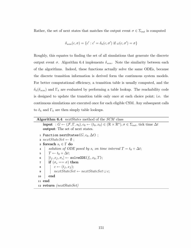
Rather, the set of next states that matches the output event � 2 �out is computed
�scm(c; �) = fc0 : c0 = �h(c; �0) if !(c; �0) = �g
Roughly, this equates to �nding the set of all simulations that generate the discrete
output event �. Algorithm 6.4 implements �scm. Note the similarity between each
of the algorithms. Indeed, these functions actually solve the same ODEs, because
the discrete transition information is derived form the continuous system models.
For better computational e¢ ciency, a transition table is usually computed, and the
�h(�scm) and �h are evaluated by performing a table lookup. The reachability code
is designed to update the transition table only once at each choice point; i.e. the
continuous simulations are executed once for each eligible CSM. Any subsequent calls
to �h and �h are then simply table lookups.
Algorithm 6.4: nextStates method of the SCM classinput : G (F ;�; s0); c0 (t0; x0) 2 (R� Rn); � 2 �out; tick time �toutput: The set of next states.
Function nextStates(G; c0;�t) ;1
nextStateSet ; ;2
foreach si 2 � do3
solution of ODE posed by si on time interval T = t0 +�t;4
T t0 +�t;5
[tf ; xf ; �e] solveODE(fi; x0; T);6
if (�e == �) then7
c (tf ; xf );8
nextStateSet nextStateSet [ c;9
end10
end11
return (nextStateSet)12
151
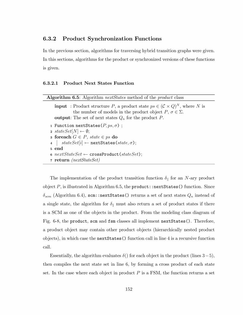
6.3.2 Product Synchronization Functions
In the previous section, algorithms for traversing hybrid transition graphs were given.
In this sections, algorithms for the product or synchronized versions of these functions
is given.
6.3.2.1 Product Next States Function
Algorithm 6.5: Algorithm nextStates method of the product class
input : Product structure P , a product state ps 2 (C �Q)N , where N isthe number of models in the product object P , � 2 �:
output: The set of next states Qn for the product P .
Function nextStates(P; ps; �) ;1
stateSet[N ] ;;2
foreach G 2 P , state 2 ps do3
stateSet[i] nextStates(state; �);4
end5
nextStateSet crossProduct(stateSet);6
return (nextStateSet)7
The implementation of the product transition function �k for an N -ary product
object P , is illustrated in Algorithm 6.5, the product::nextStates() function. Since
�scm (Algorithm 6.4), scm::nextStates() returns a set of next states Qn instead of
a single state, the algorithm for �k must also return a set of product states if there
is a SCM as one of the objects in the product. From the modeling class diagram of
Fig. 6-8, the product, scm and fsm classes all implement nextStates(). Therefore,
a product object may contain other product objects (hierarchically nested product
objects), in which case the nextStates() function call in line 4 is a recursive function
call.
Essentially, the algorithm evaluates �() for each object in the product (lines 3�5),
then compiles the next state set in line 6, by forming a cross product of each state
set. In the case where each object in product P is a FSM, the function returns a set
152
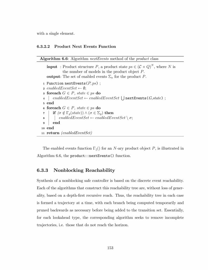
with a single element.
6.3.2.2 Product Next Events Function
Algorithm 6.6: Algorithm nextEvents method of the product class
input : Product structure P , a product state ps 2 (C �Q)N , where N isthe number of models in the product object P .
output: The set of enabled events �n for the product P .
Function nextEvents(P; ps) ;1
enabledEventSet ;;2
foreach G 2 P , state 2 ps do3
enabledEventSet enabledEventSetSnextEvents(G,state) ;4
end5
foreach G 2 P , state 2 ps do6
if (� =2 �g(state)) ^ (� 2 �g) then7
enabledEventSet enabledEventSet n �;8
end9
end10
return (enabledEventSet)11
The enabled events function �k() for an N -ary product object P , is illustrated in
Algorithm 6.6, the product::nextEvents() function.
6.3.3 Nonblocking Reachability
Synthesis of a nonblocking safe controller is based on the discrete event reachability.
Each of the algorithms that construct this reachability tree are, without loss of gener-
ality, based on a depth-�rst recursive reach. Thus, the reachability tree in each case
is formed a trajectory at a time, with each branch being computed temporarily and
pruned backwards as necessary before being added to the transition set. Essentially,
for each lookahead type, the corresponding algorithm seeks to remove incomplete
trajectories, i.e. those that do not reach the horizon.
153
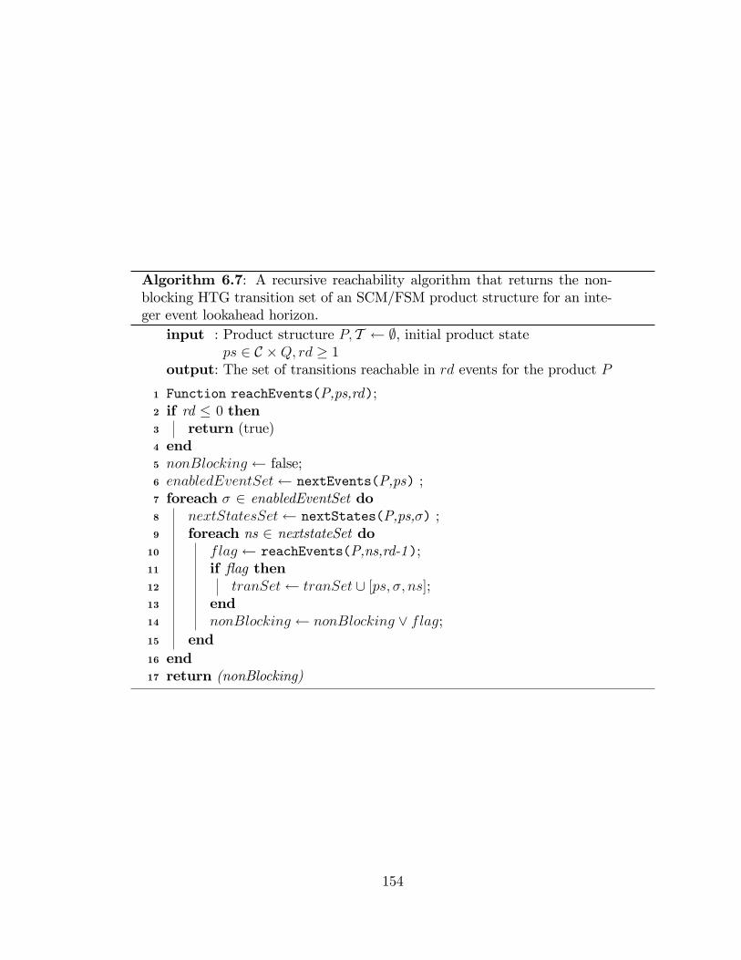
Algorithm 6.7: A recursive reachability algorithm that returns the non-blocking HTG transition set of an SCM/FSM product structure for an inte-ger event lookahead horizon.
input : Product structure P; T ;, initial product stateps 2 C �Q; rd � 1
output: The set of transitions reachable in rd events for the product P
Function reachEvents(P,ps,rd);1
if rd � 0 then2
return (true)3
end4
nonBlocking false;5
enabledEventSet nextEvents(P,ps) ;6
foreach � 2 enabledEventSet do7
nextStatesSet nextStates(P,ps,�) ;8
foreach ns 2 nextstateSet do9
flag reachEvents(P,ns,rd-1);10
if �ag then11
tranSet tranSet [ [ps; �; ns];12
end13
nonBlocking nonBlocking _ flag;14
end15
end16
return (nonBlocking)17
154
6.3.3.1 Event Reachability
The controller is constructed from the product of plant and speci�cation models
using a modi�ed reachability sweep (Algorithm 6.7). This recursive function takes
arguments of a product model object, a product state object, and the lookahead
horizon. This algorithm demonstrates a limited lookahead depth-�rst reachability. In
this case, the lookahead horizon is speci�ed by the number of events, the rd parameter
in the function call. The function terminates when every branch of the reachability
has been explored, either reaching the event lookahead or not. Providing that there
exists at least one complete trajectory, the function will terminate, returning a status
of boolean true, indicating that the reachability is non-empty. The function constructs
a transition set TR for the graph of the reachable controlled state space. Transitions
are only placed in the transition set as they are veri�ed to be non-blocking. This
requires that the algorithm traverse all the way to the lookahead horizon to verify
that a trajectory is complete. Thus, the transition set is built from the lookahead
horizon backwards in this technique.
6.3.3.2 Time Reachability
As an alternative, the lookahead horizon of the reachability can be speci�ed as a
time horizon in terms of simulation time intervals, �t, represented by the event label
tick. In Algorithm 6.8, the reachDepth parameter of the productReach function now
speci�es the number of tick events for the lookahead horizon. The recursive function
call decrements rd only if the enabled event is a tick. If the event is not a tick,
the recursive call is made with rd unchanged. This function will only terminate if
all trajectories are nonzeno, since if time is not able to advance, then the function
will call itself ad in�nitum. Assuming that the function does terminate, the resulting
transition set will consist of only those trajectories having rd tick events in each
generated string.
The time horizon can also be speci�ed in dense time T � t. The algorithm will not
155
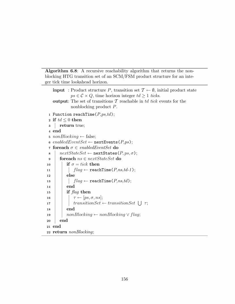
Algorithm 6.8: A recursive reachability algorithm that returns the non-blocking HTG transition set of an SCM/FSM product structure for an inte-ger tick time lookahead horizon.
input : Product structure P , transition set T ;, initial product stateps 2 C �Q, time horizon integer td � 1 ticks.
output: The set of transitions T reachable in td tick events for thenonblocking product P .
Function reachTime(P,ps,td);1
if td � 0 then2
return true;3
end4
nonBlocking false;5
enabledEventSet nextEvents(P,ps);6
foreach � 2 enabledEventSet do7
nextStateSet nextStates(P; ps; �);8
foreach ns 2 nextStateSet do9
if � = tick then10
flag reachTime(P,ns,td-1);11
else12
flag reachTime(P,ns,td);13
end14
if �ag then15
� [ps; �; ns];16
transitionSet transitionSetS
� ;17
end18
nonBlocking nonBlocking _ flag;19
end20
end21
return nonBlocking;22
156
be presented here due to the similarity with Algorithm 6.8. Recall that the discrete
plant state is a continuous product state object consisting of the [te; xe] continuous
state xe and the simulation time te at the occurrence of the event. Essentially, the
dense time can be extracted from the plant product state. This time te can be tested
against the lookahead time T to determine if the horizon has been reached.
6.3.3.3 Combination Reachability
A combination of time and event lookahead horizons can also be utilized. Such a
combined strategy has the bene�t of assuring an upper bound that balances the
objectives of both types of lookahead schemes. It reduces complexity in the following
situations:
1. Event Lookahead: Continuous systemmodel dynamics that are slow changing
and thus generate few events (except for tick events) will terminate on a time
horizon instead of continuing until the event limit.
2. Time lookahead: continuous systemmodel dynamics and a partitioning struc-
ture that leads to dense switching behaviour (limit-cycle behaviour) will termi-
nate on the event limit instead of continuing until the time limit.
The algorithm is simply a blend of the event and time horizon reachability algo-
rithms. Essentially, the horizons are speci�ed as integers td � rd. Whichever horizon
is encountered �rst sets the returned nonblocking �ag true, indicating the complete
trajectory for this depth �rst reach to be nonblocking.
6.3.4 Fail-safe Controller Synthesis
For fail-safe control, an ESD state must be reachable (Proposition 5.4.1) from the
current system state. Algorithm 6.10 builds a transition set that is pruned according
to nonblocking and ESD state reachability rules. It also returns the nonblocking and
157
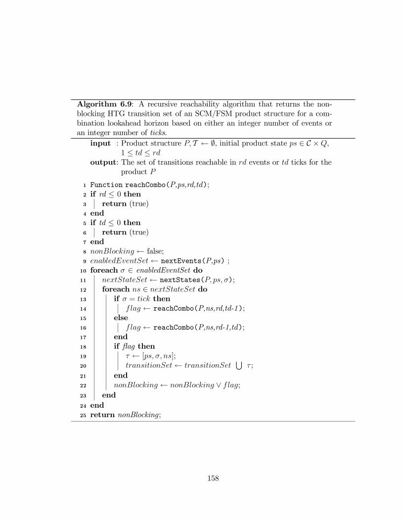
Algorithm 6.9: A recursive reachability algorithm that returns the non-blocking HTG transition set of an SCM/FSM product structure for a com-bination lookahead horizon based on either an integer number of events oran integer number of ticks.
input : Product structure P; T ;, initial product state ps 2 C �Q,1 � td � rd
output: The set of transitions reachable in rd events or td ticks for theproduct P
Function reachCombo(P,ps,rd,td);1
if rd � 0 then2
return (true)3
end4
if td � 0 then5
return (true)6
end7
nonBlocking false;8
enabledEventSet nextEvents(P,ps) ;9
foreach � 2 enabledEventSet do10
nextStateSet nextStates(P; ps; �);11
foreach ns 2 nextStateSet do12
if � = tick then13
flag reachCombo(P,ns,rd,td-1);14
else15
flag reachCombo(P,ns,rd-1,td);16
end17
if �ag then18
� [ps; �; ns];19
transitionSet transitionSetS
� ;20
end21
nonBlocking nonBlocking _ flag;22
end23
end24
return nonBlocking;25
158
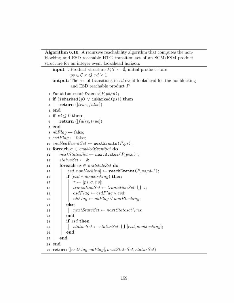
Algorithm 6.10: A recursive reachability algorithm that computes the non-blocking and ESD reachable HTG transition set of an SCM/FSM productstructure for an integer event lookahead horizon.
input : Product structure P; T ;, initial product stateps 2 C �Q; rd � 1
output: The set of transitions in rd event lookahead for the nonblockingand ESD reachable product P
Function reachEvents(P,ps,rd);1
if (isMarked(p) _ isMarked(ps)) then2
return ([true; false])3
end4
if rd � 0 then5
return ([false; true])6
end7
nbF lag false;8
esdF lag false;9
enabledEventSet nextEvents(P,ps) ;10
foreach � 2 enabledEventSet do11
nextStatesSet nextStates(P,ps,�) ;12
statusSet ;;13
foreach ns 2 nextstateSet do14
[esd; nonblocking] reachEvents(P,ns,rd-1);15
if (esd ^ nonblocking) then16
� [ps; �; ns];17
transitionSet transitionSetS
� ;18
esdF lag esdF lag _ esd;19
nbF lag nbF lag _ nonBlocking;20
else21
nextStateSet nextStateset n ns;22
end23
if esd then24
statusSet statusSetS[esd; nonblocking];25
end26
end27
end28
return ([esdF lag; nbF lag]; nextStateSet; statusSet)29
159
ESD reachable status, and a matching set of next states (or transitions). This set
of transitions, along with the nonblocking and ESD �ags, are used to choose the
next controller action (Table 5.1).The algorithm presented here is based on event
horizon reach, but can be modi�ed to be based on integer tick time, dense time, or
combination lookahead.
6.3.4.1 ESD and State Marking
ESD states must be indicated specially; in this implementation, they are calledmarked
states. The method isMarked() is implemented by subclasses of stateObject and
depObj. Thus, marking may be jointly speci�ed for individual states as well as for
models. If a model (a depObj) is marked, then all of its states are considered to
be marked. ESD marking has to retain the hierarchical structure of the product
and pstate classes; a hierarchical truth object is returned for product or pstate
classes that instantiate the isMarked() method. For example, let us look at the
hierarchical system model of Fig. 6-10. The following commands generate the logical
data structures that represent the model and state marking illustrated in Fig. 6-15:
modelMarking = isMarked(p1); %p1 is the system model
stateMarking = isMarked(ps1); %ps1 is the current product state
In line 2 of Algorithm 6.10, the logical OR (_) symbol is an overloaded opera-
tion. Without presenting the algorithm, the resulting marking is a element-wise OR
between the �branch ends�of the model and the state structures; but with the re-
quirement that the individual product object and product state object truth results
must all be true for a product model or product state to be true (AND). This special
test for marking is conducted to determine the ESD marking, and as is evident in
Fig. 6-15, for this example the result is true.
For the scm class, no states are marked internally, but discrete states of an SCM
can be designated as marked by synchronizing a FSM with the SCM to provide the
160
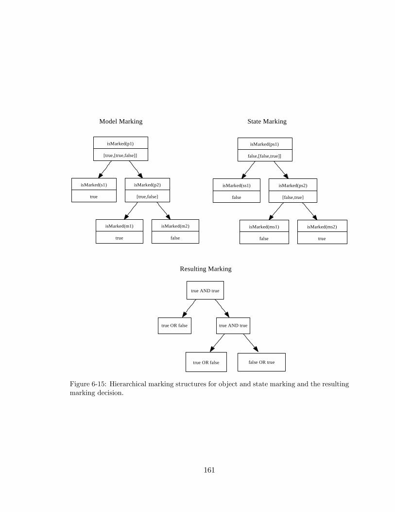
isMarked(p1)
[true,[true,false]]
isMarked(s1)
true
isMarked(p2)
[true,false]
isMarked(m1)
true
isMarked(m2)
false
isMarked(ps1)
false,[false,true]]
isMarked(ss1)
false
isMarked(ps2)
[false,true]
isMarked(ms1)
false
isMarked(ms2)
true
Model Marking State Marking
true AND true
true OR false false OR true
true AND true
true OR false
Resulting Marking
Figure 6-15: Hierarchical marking structures for object and state marking and the resultingmarking decision.
161
appropriate marking. Alternatively, as in this example, all states may be marked in
the SCM by using the object marking to always override the state marking.
6.4 Complexity
The complexity of the controller synthesis computation is of utmost importance to the
practical implementation of an online controller. In previous sections, considerable
care was taken to outline the various approaches to reducing complexity, including
lazy computation, and limited lookahead. This section will outline the expected space
and time complexity of implementing the hybrid controller synthesis.
Essentially, the process of online synthesis consists of generating a locally safe con-
troller repeatedly at di¤erent instances in space, and more importantly, time. The
controller is assembled in a just-in-time fashion, so it is essential that the computation
can be computed reliably, in a �nite amount of time. The controller is represented
by a directed acyclic graph that is the result of the product of a switched continuous
models and one or more �nite state models. The plant, represented by the switched
continuous model, can be "�attened", that is, its reachable state space can be cal-
culated on a reduced time horizon combined with the limited switching framework
(choice points) to produce a �nite state model. In §4.6, the cardinality of the reach-
able state space R of a SCM was derived for Case I and Case II switching (Eq. 4.7
and Eq. 4.4). Since there exists a transition in the HTG for every xi 2 R, the number
of transitions is as follows:
pq + 1 � jTRj �rpq+1 � 1r � 1 ; r > 1
where q is the length of the longest SC trajectory (the maximum reach depth)
and r is the number of possible continuous system models (control actions) available
at any choice point. Since both q and r are a function of the speci�cation model,
the plant model and the particular product state at the moment the controller is to
162
be computed, it is not possible to �nd the exact controller size, but it is possible to
classify the order of the calculation in space and time. the following sections examine
the complexity for a system modeled by a single SCM.
6.4.1 Constant Event Reach (Plant)
The constant event reach has a �xed number of states which is determined by integer q;
the reach depth, and integer r; the branching factor (the number of enabled continuous
system models). Thus, the number of transitions in the graph that implements the
�nite state model is
jTRj =rq+1 � 1r � 1 , r > 1
providing that there are exactly r choices at each choice point.
Lemma 6.4.1 (Space Complexity Reach (Events)) Let G = (F;�; s0) be a switched
continuous model. The space complexity of the reachability calculation with constant
event horizon (reach depth) is polynomial in r.
Proof. With the number of events in any complete switched continuous trajectory
(string) j�j = q �xed, the number of transitions in the HTG is a function of r
jTRj = f(r) =rq+1 � 1r � 1 , r > 1
with r large, this converges to rq. Therefore for q > 1, the space complexity is
O(rq)which is polynomial in r.
6.4.2 Constant Time Reach (Plant)
With constant time reach, the maximum reach depth in events pq; is not consistent
for each SC trajectory � 2 R, and is unpredictable depending upon the dynamics
and partitioning structure of the SC model G = (F ;�; s0). Recall that the reachable
163
state space R of an SC model of a �xed-time horizon of p �t , with �nite number of
partition switches per time interval of q = j�j has an upper bound of
jRj � rpq+1 � 1r � 1 , r > 1
which corresponds directly to the number transitionsjTRj in the HTG of G.
Lemma 6.4.2 (Space Complexity Reach (Breadth)) Let G = (F;�; s0) be a
switched continuous model. The space complexity of the reachability calculation with
a �xed number of model choices (reach breadth) is exponential in pq.
Proof. Let pq = q0. Clearly with r constant, the number of states in the reacha-
bility graph, N , is a function of q0
jTRj = f(q0) =rq
0+1 � 1r � 1 ; r > 1
Therefore, the worst-case space complexity is O(rq0), that is exponential in pq.
6.4.3 Complexity With Control
This section examines the computational cost of computing a controller. The number
of possible branches that can be made at any choice point is dictated by the number
of available dynamics r = j�j, and by the number of these choices that are disabled
by the speci�cation. This disablement is unpredictable and is determined by how
�tight�the speci�cation is. Any other synchronous model connected to the plant may
also constrain the plant branching behaviour, even though it may not necessarily be
considered as part of the speci�cation.
� State complexity of the controller has an upper bound which is polynomial in r,
and exponential in q. In practice, however, due to the discrete-event interaction
of the SCMwith other plant and speci�cation models, the complexity will always
be less.
164
� Time complexity for reachability of a directed graph is O(N), in the number of
nodes or states of the controller, N . Therefore, time complexity for forming the
controller, in terms of q and r; is essentially the same complexity as the state
complexity. Therefore time complexity is at worst, exponential, but will always
be better depending on the interaction of the SCM with other models.
� A �tight�speci�cation helps to reduce complexity. The implication of a "tight"
speci�cation however, is that a larger set of plant behaviours will be disabled.
This e¤ectively reduces the available control choices, increasing the likelihood
of blocking, and an unwarranted emergency shutdown.
6.4.4 Empirical Complexity
It is not possible to analytically predict the exact complexity of controller synthesis
for a particular system model, but it is possible to evaluate it empirically.
To demonstrate complexity reduction, we will use the tank control example of
§4.9 again. The plot of Fig. 6-16 shows the controller size for this example (at the
same initial state) for a range of event lookahead horizons. Plotted on a logarithmic
scale, the number of transitions in the uncontrolled plant increases by approximately
one order of magnitude for an increase in lookahead horizon by 2 events. For this
example, there is a considerable decrease in controller size due to the inclusion of the
speci�cation; an approximate curve �t has been applied (in blue) to the controller
data.
The size of the controller also varies depending on the initial condition; a simula-
tion of the tank control example repeated for 50 controller updates, shows a consid-
erable variation of the controller size as the controller is propagated (Fig. 6-17).
165
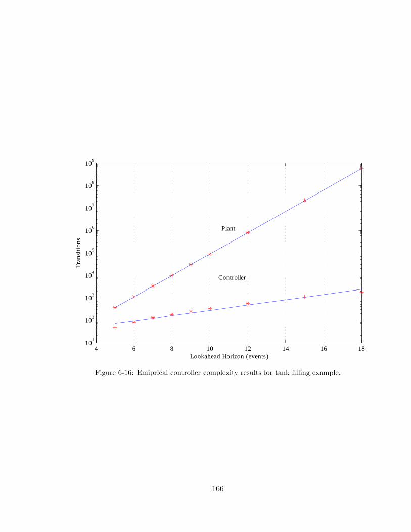
4 6 8 10 12 14 16 18101
102
103
104
105
106
107
108
109
Tran
sitio
ns
Lookahead Horizon (events)
Plant
Controller
Figure 6-16: Emiprical controller complexity results for tank �lling example.
166
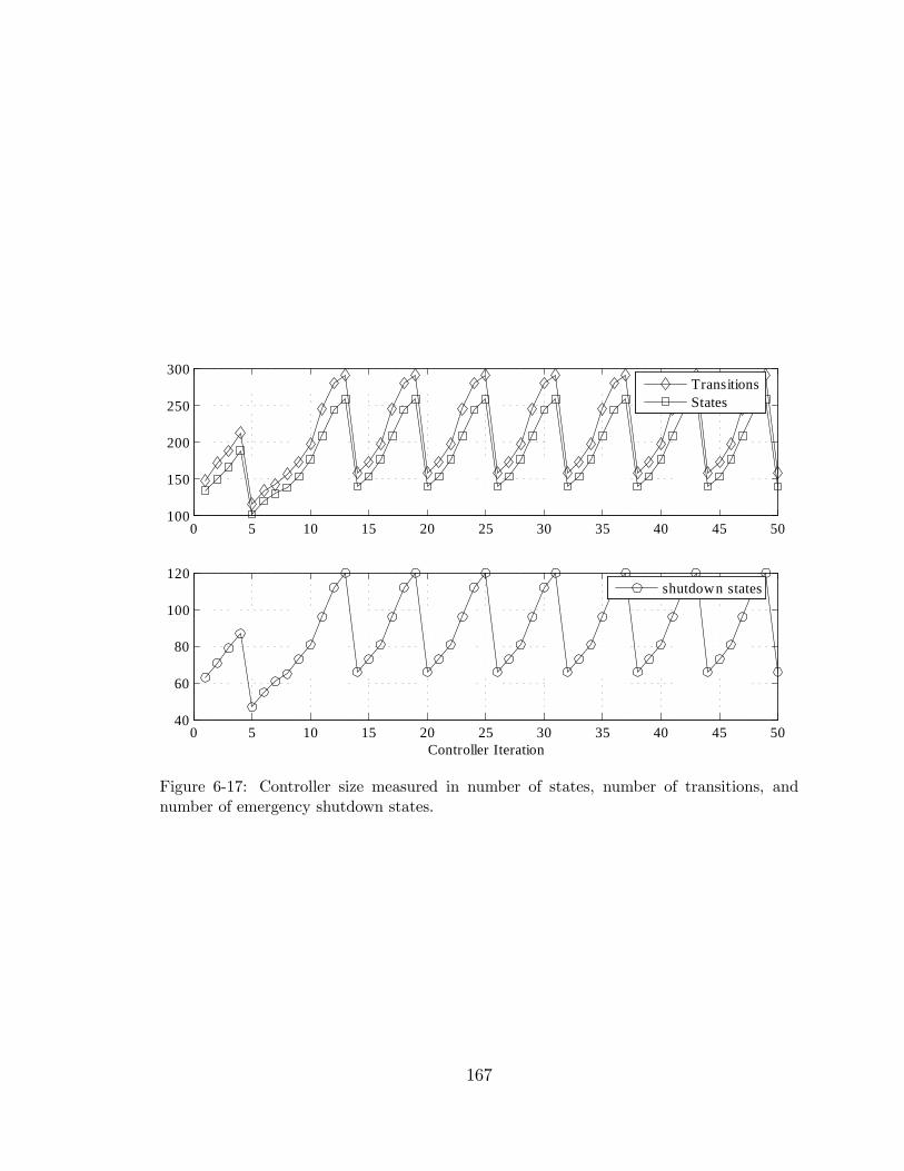
0 5 10 15 20 25 30 35 40 45 50100
150
200
250
300TransitionsStates
0 5 10 15 20 25 30 35 40 45 5040
60
80
100
120
Controller Iteration
shutdown states
Figure 6-17: Controller size measured in number of states, number of transitions, andnumber of emergency shutdown states.
167
6.5 Summary
This chapter has taken the theoretical concepts of the preceding chapters and de-
scribed one possible implementation. The controllers that we wish to synthesize are
implemented online (i.e. a real time environment); thus the entire computational
framework has been designed to e¢ ciently achieve this goal. The primary challenge
is to manage the computational complexity of the controller synthesis, since the con-
troller is to be implemented online. We achieve a signi�cant reduction in computa-
tional complexity by combining the speci�cation with the controller at design time.
The hierarchical modeling framework allows for a �lazy�or just in time assembly of
the controller from its constituent models. The reduction in complexity comes from
the fact that illegal traces can be eliminated without expanding the entire �attened
state space of the model. In fact, since we are dealing with a hybrid model that
theoretically has an in�nite state space, the entire model is impossible to compute.
Therefore, a limited lookahead horizon technique is used to compute the reachable
state space. The lookahead horizon may be speci�ed in events, integer (tick) time,
dense time, or a combination of these.
A software package called HySynth has been developed to help evaluate the ef-
fectiveness and the practicality of the theoretical approach. The HySynth computa-
tional engine exploits object oriented programming techniques to implement the lazy
computational strategy. Written for the Matlab environment, the modeling frame-
work can leverage the wide range of general and special purpose numerical simulation
toolboxes available for Matlab.
In the next chapter, we will examine speci�c application examples, in which
HySynth is used to formulate hybrid system models, compute discrete event su-
pervisory controllers, and to simulate the closed-loop system behaviour.
168
Chapter7Applications
This chapter presents two application examples that demonstrate in more detail,
the system modeling process and controller synthesis for hybrid systems using
the switched continuous model. The HySynth software package has been used to
model, synthesize and simulate the controlled systems that are presented here. The
�rst example, the control of liquid in two tanks, is a common benchmark hybrid con-
trol design problem. The second example is a detailed industrial example based on
the control of a vessel and its associated systems. This example in particular demon-
strates the utility of the control techniques developed in this document, and represents
the �rst time a hybrid control design has been attempted for this application.
7.1 Tank Level Control
Recall the example of §4.9 (p.82) in which a SCM was developed for a system consist-
ing of a tank of some �uid. In this example, we will develop a speci�cation, synthesize
an online controller and simulate its operation. This example points out the basics
of control synthesis and illustrates the use of the HySynth software package.
With the plant modeled as a SCM, the desired closed loop behavior can be speci�ed
in the form of �nite state machines. The desired behavior is modeled by the �nite state
169
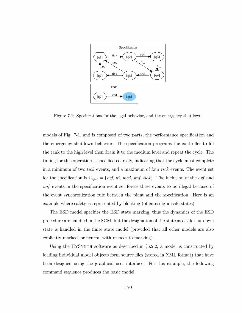
ESD
Specification
[q7] [q8]esd
[q1] [q2]tick [q3]tick
[q4]
hi_hi_
[q5] tick
med
[q6] tick
med
Figure 7-1: Speci�cations for the legal behavior, and the emergency shutdown.
models of Fig. 7-1, and is composed of two parts; the performance speci�cation and
the emergency shutdown behavior. The speci�cation programs the controller to �ll
the tank to the high level then drain it to the medium level and repeat the cycle. The
timing for this operation is speci�ed coarsely, indicating that the cycle must complete
in a minimum of two tick events, and a maximum of four tick events. The event set
for the speci�cation is �spec = fovf, hi, med, unf, tickg. The inclusion of the ovf and
unf events in the speci�cation event set forces these events to be illegal because of
the event synchronization rule between the plant and the speci�cation. Here is an
example where safety is represented by blocking (of entering unsafe states).
The ESD model speci�es the ESD state marking, thus the dynamics of the ESD
procedure are handled in the SCM, but the designation of the state as a safe shutdown
state is handled in the �nite state model (provided that all other models are also
explicitly marked, or neutral with respect to marking).
Using the HySynth software as described in §6.2.2, a model is constructed by
loading individual model objects form source �les (stored in XML format) that have
been designed using the graphical user interface. For this example, the following
command sequence produces the basic model:
170
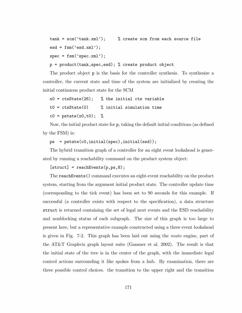
tank = scm(�tank.xml�); % create scm from each source file
esd = fsm(�esd.xml�);
spec = fsm(�spec.xml�);
p = product(tank,spec,esd); % create product object
The product object p is the basis for the controller synthesis. To synthesize a
controller, the current state and time of the system are initialized by creating the
initial continuous product state for the SCM
x0 = ctsState(26); % the initial cts variable
t0 = ctsState(0) % initial simulation time
c0 = pstate(x0,t0); %
Now, the initial product state for p, taking the default initial conditions (as de�ned
by the FSM) is:
ps = pstate(c0,initial(spec),initial(esd));
The hybrid transition graph of a controller for an eight event lookahead is gener-
ated by running a reachability command on the product system object:
[struct] = reachEvents(p,ps,8);
The reachEvents() command executes an eight-event reachability on the product
system, starting from the argument initial product state. The controller update time
(corresponding to the tick event) has been set to 90 seconds for this example. If
successful (a controller exists with respect to the speci�cation), a data structure
struct is returned containing the set of legal next events and the ESD reachability
and nonblocking status of each subgraph. The size of this graph is too large to
present here, but a representative example constructed using a three event lookahead
is given in Fig. 7-2. This graph has been laid out using the neato engine, part of
the AT&T Graphviz graph layout suite (Gansner et al. 2002). The result is that
the initial state of the tree is in the center of the graph, with the immediate legal
control actions surrounding it like spokes from a hub. By examination, there are
three possible control choices. the transition to the upper right and the transition
171
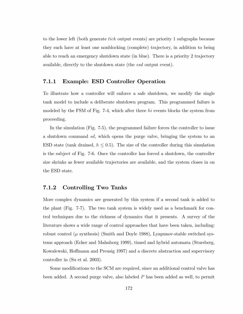
to the lower left (both generate tick output events) are priority 1 subgraphs because
they each have at least one nonblocking (complete) trajectory, in addition to being
able to reach an emergency shutdown state (in blue). There is a priority 2 trajectory
available, directly to the shutdown state (the esd output event).
7.1.1 Example: ESD Controller Operation
To illustrate how a controller will enforce a safe shutdown, we modify the single
tank model to include a deliberate shutdown program. This programmed failure is
modeled by the FSM of Fig. 7-4, which after three hi events blocks the system from
proceeding.
In the simulation (Fig. 7-5), the programmed failure forces the controller to issue
a shutdown command sd, which opens the purge valve, bringing the system to an
ESD state (tank drained, h � 0:5). The size of the controller during this simulation
is the subject of Fig. 7-6. Once the controller has forced a shutdown, the controller
size shrinks as fewer available trajectories are available, and the system closes in on
the ESD state.
7.1.2 Controlling Two Tanks
More complex dynamics are generated by this system if a second tank is added to
the plant (Fig. 7-7). The two tank system is widely used as a benchmark for con-
trol techniques due to the richness of dynamics that it presents. A survey of the
literature shows a wide range of control approaches that have been taken, including:
robust control (� synthesis) (Smith and Doyle 1988), Lyapunov-stable switched sys-
tems approach (Ecker and Malmborg 1999), timed and hybrid automata (Stursberg,
Kowalewski, Ho¤mann and Preusig 1997) and a discrete abstraction and supervisory
controller in (Su et al. 2003).
Some modi�cations to the SCM are required, since an additional control valve has
been added. A second purge valve, also labeled P has been added as well, to permit
172
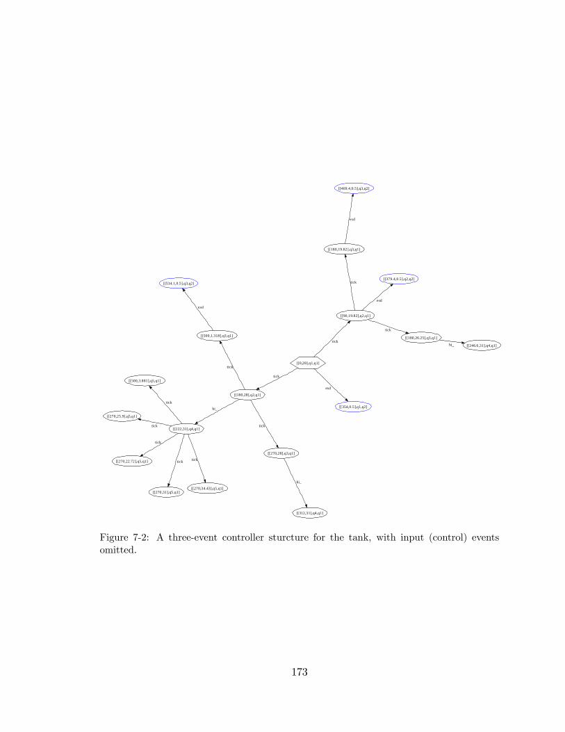
[[0,28],q1,q1]
[[180,28],q2,q1]
tick
[[354,0.5],q1,q2]
esd
[[90,19.82],q2,q1]
tick
[[222,31],q4,q1]
hi_
[[270,28],q3,q1]
tick
[[500,1.318],q3,q1]
tick
[[180,19.82],q3,q1]
tick
[[180,26.25],q3,q1]
tick
[[379.4,0.5],q2,q2]
esd
[[469.4,0.5],q3,q2]
esd
[[246.6,31],q4,q1]hi_
[[270,22.72],q5,q1]
tick
[[270,25.9],q5,q1]
tick
[[270,31],q5,q1]
tick
[[270,34.43],q5,q1]
tick
[[500,3.881],q5,q1]
tick
[[312,31],q4,q1]
hi_
[[534.1,0.5],q3,q2]
esd
Figure 7-2: A three-event controller sturcture for the tank, with input (control) eventsomitted.
173
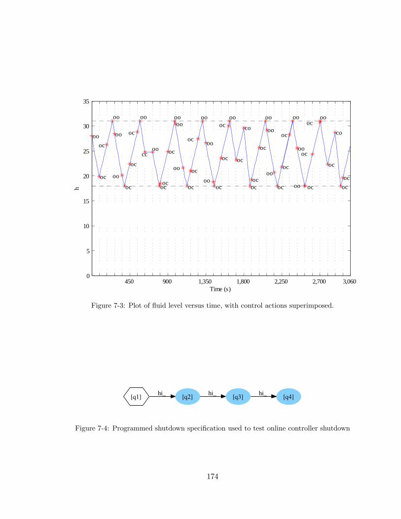
450 900 1,350 1,800 2,250 2,700 3,0600
5
10
15
20
25
30
35
oo
oc
oc
oo
oo
oo
oc
oc
oc
oo
ccoo
ococ
oc
oooo
oo oc
oc
oo
oo
oo
oc
ocoo
oc
co
ococ
oc
oo
oo
oo
oc
oc
oc
oo
oo
oo oc
oc
ocoo
oc
co
ococ
Time (s)
h oc oc
Figure 7-3: Plot of �uid level versus time, with control actions superimposed.
[q1] [q2]hi_
[q3]hi_
[q4]hi_
Figure 7-4: Programmed shutdown speci�cation used to test online controller shutdown
174
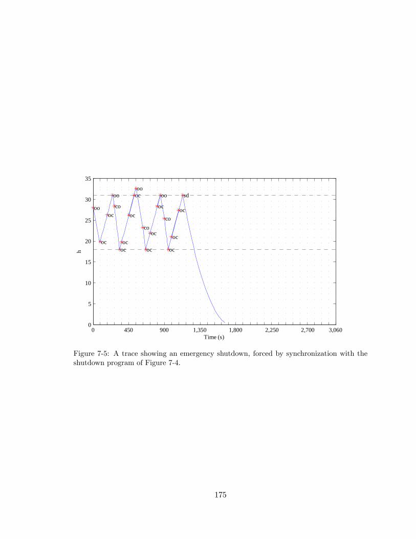
0 450 900 1,350 1,800 2,250 2,700 3,0600
5
10
15
20
25
30
35
oo
oc
oc
oo
co
ococ
oc
ocoo
co
oc
oc
oc
oo
co
oc
oc
oc
sd hi
med
Time (s)
h
Figure 7-5: A trace showing an emergency shutdown, forced by synchronization with theshutdown program of Figure 7-4.
175
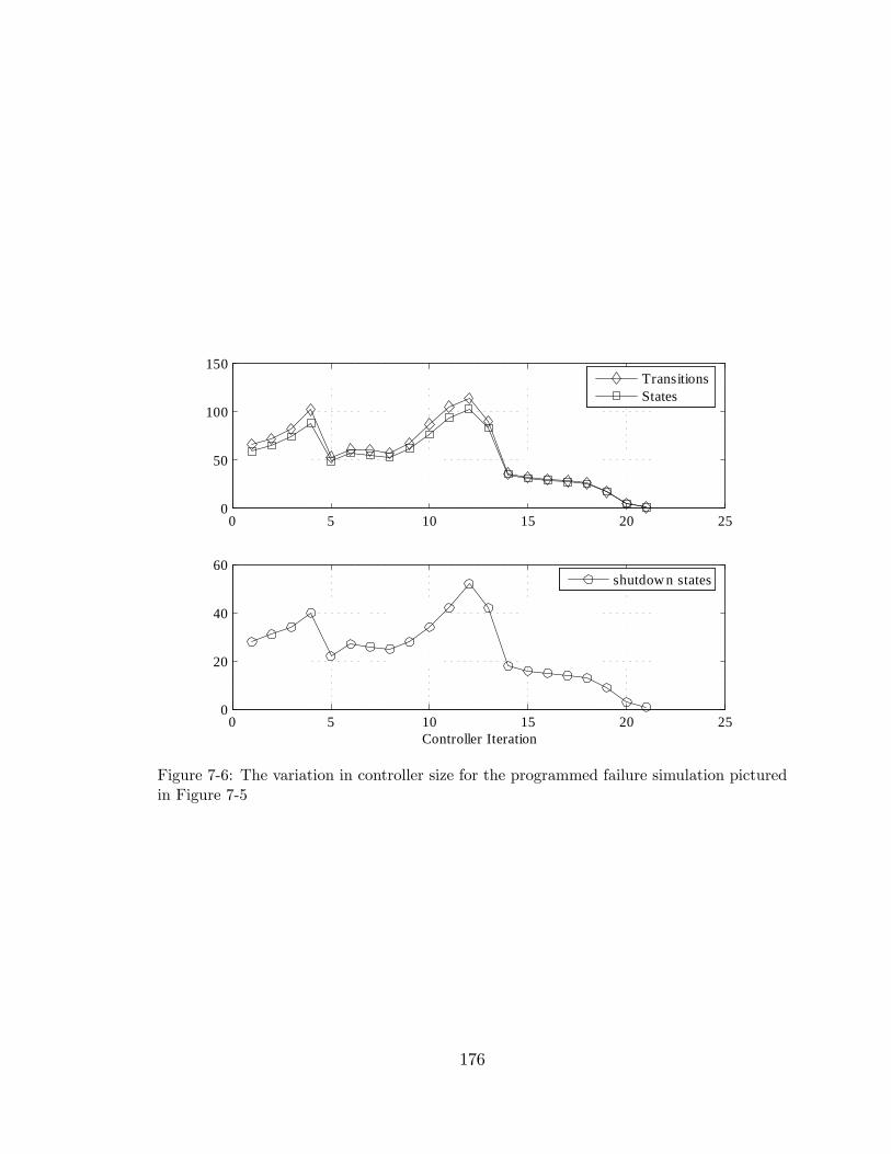
0 5 10 15 20 250
50
100
150TransitionsStates
0 5 10 15 20 250
20
40
60
Controller Iteration
shutdow n states
Figure 7-6: The variation in controller size for the programmed failure simulation picturedin Figure 7-5
176

1h
1q
12q
1V
2V
ovf1high1
med1
esd1
P
unf1
2h
2q
3V
ovf2high2
med2
esd2
P
unf2
Figure 7-7: Two tank system schematic.
177
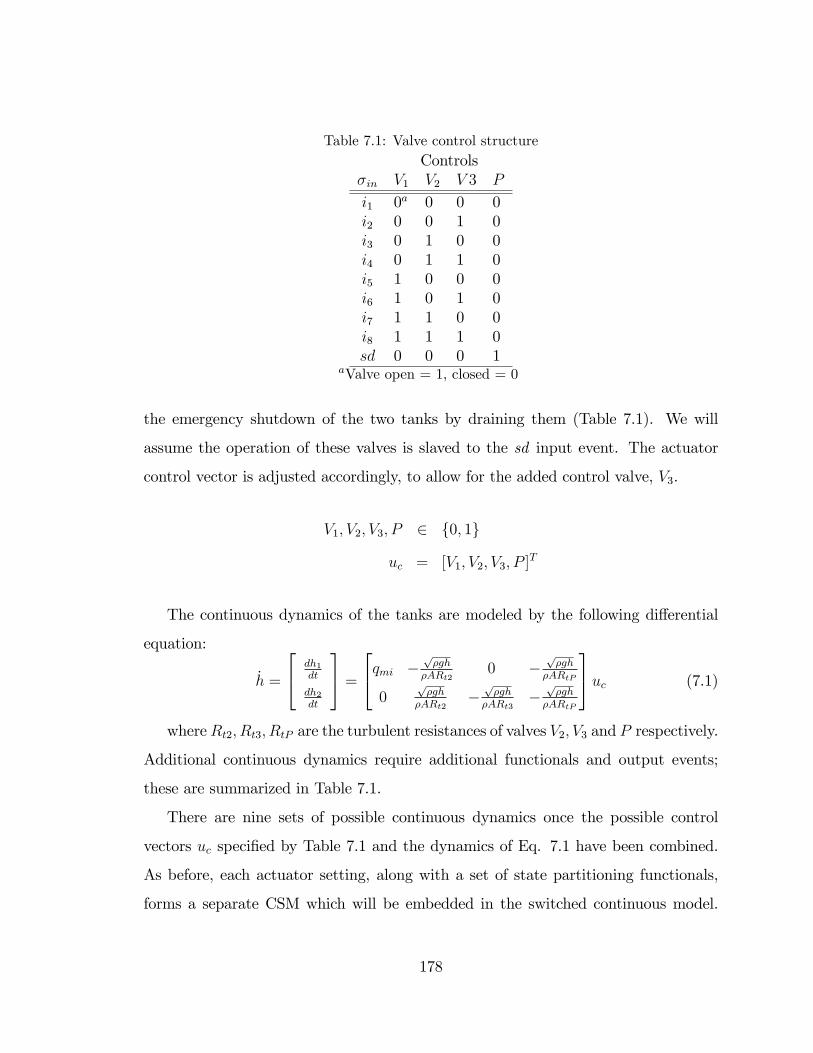
Table 7.1: Valve control structureControls
�in V1 V2 V 3 P
i1 0a 0 0 0i2 0 0 1 0i3 0 1 0 0i4 0 1 1 0i5 1 0 0 0i6 1 0 1 0i7 1 1 0 0i8 1 1 1 0sd 0 0 0 1
aValve open = 1, closed = 0
the emergency shutdown of the two tanks by draining them (Table 7.1). We will
assume the operation of these valves is slaved to the sd input event. The actuator
control vector is adjusted accordingly, to allow for the added control valve, V3.
V1; V2; V3; P 2 f0; 1g
uc = [V1; V2; V3; P ]T
The continuous dynamics of the tanks are modeled by the following di¤erential
equation:
_h =
24 dh1dt
dh2dt
35 =24qmi � p
�gh�ARt2
0 �p�gh
�ARtP
0p�gh
�ARt2�
p�gh
�ARt3�
p�gh
�ARtP
35uc (7.1)
whereRt2; Rt3; RtP are the turbulent resistances of valves V2; V3 and P respectively.
Additional continuous dynamics require additional functionals and output events;
these are summarized in Table 7.1.
There are nine sets of possible continuous dynamics once the possible control
vectors uc speci�ed by Table 7.1 and the dynamics of Eq. 7.1 have been combined.
As before, each actuator setting, along with a set of state partitioning functionals,
forms a separate CSM which will be embedded in the switched continuous model.
178

Table 7.2: Output events, with associated functionals and hypersurface crossing directionsfor the two tank control synthesis problem.
�out Functional Zero-crossing Alarmovf1 F1(h) = h1 � 33 " over �lled (tank 1)hi1 F2(h) = h1 � 31 " highmed1 F3(h) = h1 � 18 # mediumunf1 F4(h) = h1 � 15 # under �lledovf2 F5(h) = h2 � 33 " over �lled (tank 2)hi2 F6(h) = h2 � 31 " highmed2 F7(h) = h2 � 27 # mediumunf2 F8(h) = h2 � 20 # under �lledesd F9(h) = (h1 � 0:5) ^ (h2 � 0:5) # emergency shutdown
The CSMs corresponding to input events i1 to i8 share the same set of functionals
1 = fF1; F2; F3; F4; F5; F6; F7; F8g and the CSM for emergency shutdown operation
(both purge valves P open) has 2 = fF9g: The functionals are de�ned in Table
7.2 along with their associated output events. In this case, the esd output event is
signaled when both tanks are drained (h1; h2 � 0:5).
The speci�cation for this system will be similar to the single-tank system; we wish
both tanks to cycle between an upper (hi event) and lower limit (med event). The
�ll/drain cycle timing is speci�ed in coarse (tick) time 2�t � t � 4�t, where �t = 90
seconds.
In Fig. 7-8 the �nite state models are given for this speci�cation. The HySynth
commands to build the model are as follows:
s1 = fsm(�spec1.xml�); %load the tank 1 specification
s2 = fsm(�spec2.xml�); %load the tank 2 specification
spec = product(s1,s2); %create the spec product object
plant = scmodel(�tank.xml�); %two tanks SC model
esd = fsm(�esd.xml�); % esd specification
p1 = product(plant,spec,esd); % Create the controller model
The result of these commands is the product model structure of Fig. 7-9. A
179

ESD
Specification Tank #2
Specification Tank #1
[q10] [q11]esd
[q1] [q2]tick
[q3]tick
[q4]hi2
hi2
[q5] tick
med2[q6] tick
med2
[q1] [q2]tick
[q3]tick
[q4]hi1
hi1
[q5] tick
med1[q6] tick
med1
Figure 7-8: The speci�cation models for the two tank level controller.
p1
product(plant,spec,esd)
plant
scm('tank.xml')
spec
product(s1,s2)
esd
fsm('esd.xml')
s1
fsm('spec1.xml')
s2
fsm('spec2.xml')
Figure 7-9: The hierarchical model structure for the two tank controller synthesis.
180

0 500 1000 1500 2000 2500 3000 3500 4000 4500
15
20
25
30
35
Time (s)
h 1ovf 1
unf1
0 500 1000 1500 2000 2500 3000 3500 4000 4500
15
20
25
30
35
h 2
ovf 2
unf2
Figure 7-10: Simulation of the online controller using a 5-event lookahead horizon andrandom control choice.
controller synthesis based on an event horizon reach of 5 events was used for the
simulation. The controller advances using a random selection of control actions from
the available legal subset of input events (as determined by the online controller) at
each of 100 choice points. The resulting control performance is pictured in Fig. 7-10,
in which the state variables, h1 and h2 have been plotted versus time. The top trace
is h1, the level of tank 1 and the lower trace is h2; the �uid level in tank 2. The
choice points, where the controller has acted, are indicated by diamond markers on
the traces.
In Fig. 7-11, a section of this simulation has been enlarged with the two traces
overlapped to show the time history in more detail, with h1 the blue trace, and h2
181
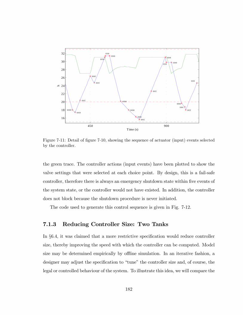
450 900
16
18
20
22
24
26
28
30
32
ooo
coc
occ
ooooco
occ
ooc
occ
oco
ccocoo
ooo
ooo
oococc
occ
coo
cco coo
ooccoc
occ
cco
ooo
cco ooo
ooc
coo
ooo
oco
occ
occ
ooo
coc
ooo
ooo
ooooco
occ
oco
coo
ooc
coo
oco
ccoocc
occ
coo
oococc
cco coo
occocc
ooc
occ
ooo
cco coo
coc
oocooo
occ
occ
ccooccooc
ooo
cco coo
oocooc
occ
oco
oco
ooo
coc
ooo
ooo
oco
ooo
occ
occ
coc
ooo
coo
oco
oco
occ
occcoc
ooo
T ime (s)
h
unf 1
unf 2
ovf 1/2
Figure 7-11: Detail of �gure 7-10, showing the sequence of actuator (input) events selectedby the controller.
the green trace. The controller actions (input events) have been plotted to show the
valve settings that were selected at each choice point. By design, this is a fail-safe
controller, therefore there is always an emergency shutdown state within �ve events of
the system state, or the controller would not have existed. In addition, the controller
does not block because the shutdown procedure is never initiated.
The code used to generate this control sequence is given in Fig. 7-12.
7.1.3 Reducing Controller Size: Two Tanks
In §6.4, it was claimed that a more restrictive speci�cation would reduce controller
size, thereby improving the speed with which the controller can be computed. Model
size may be determined empirically by o ine simulation. In an iterative fashion, a
designer may adjust the speci�cation to �tune�the controller size and, of course, the
legal or controlled behaviour of the system. To illustrate this idea, we will compare the
182
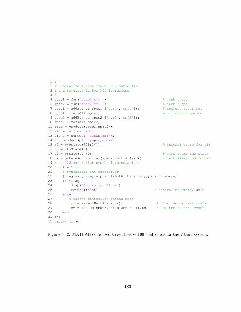
1 % 2 % Program to synthesize a DES controller 3 % and simulate it for 100 iterations 4 % 5 spec1 = fsm( 'spec1.xml' % tank 1 spec 6 spec2 = fsm( 'spec2.xml' % tank 2 spec 7 spec1 = addEvents(spec1,[ 'ovf1' 'unf1' % augment event set 8 spec1 % all states marked 9 spec2 = addEvents(spec2,[ 'ovf2' 'unf2'10 spec2
11 spec12 esd = fsm( 'esd.xml'13 plant = scmodel( 'tanks.xml'14 p15 x0 % initial state for sim16 t0 = ctsState(0)17 c0 = pstate(t0,x0) % time stamp the state18 ps = pstate(c0,initial(spec),initial(esd)) % initialize controller19 % do 100 controller synthesis/simulations20 for i = 1:10021 % synthesize the controller22
23 if ~flag24 disp( 'Controller Block' )25 return (false) % controller empty, quit26 else27 % Choose controller action here28 % pick random next state29 ev = lookupInputEvent(plant,ps(i),ps) % get the control event30 end 31 end32 return (flag)
Figure 7-12: MATLAB code used to synthesize 100 controllers for the 2 tank system.
183
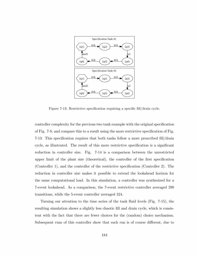
Specification Tank #2
Specification Tank #1
[q1] [q2]tick [q3]tick
[q4]
hi2
[q5] tick[q6] tick
med2
[q1] [q2]tick [q3]tick
[q4]
hi1
[q5] tick[q6] tick
med1
Figure 7-13: Restrictive speci�cation requiring a speci�c �ll/drain cycle.
controller complexity for the previous two tank example with the original speci�cation
of Fig. 7-8, and compare this to a result using the more restrictive speci�cation of Fig.
7-13. This speci�cation requires that both tanks follow a more prescribed �ll/drain
cycle, as illustrated. The result of this more restrictive speci�cation is a signi�cant
reduction in controller size. Fig. 7-14 is a comparison between the unrestricted
upper limit of the plant size (theoretical), the controller of the �rst speci�cation
(Controller 1), and the controller of the restrictive speci�cation (Controller 2). The
reduction in controller size makes it possible to extend the lookahead horizon for
the same computational load. In this simulation, a controller was synthesized for a
7-event lookahead. As a comparison, the 7-event restrictive controller averaged 290
transitions, while the 5-event controller averaged 324.
Turning our attention to the time series of the tank �uid levels (Fig. 7-15), the
resulting simulation shows a slightly less chaotic �ll and drain cycle, which is consis-
tent with the fact that there are fewer choices for the (random) choice mechanism.
Subsequent runs of this controller show that each run is of course di¤erent, due to
184
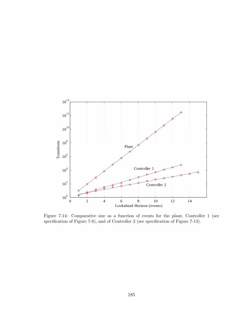
0 2 4 6 8 10 12 14100
102
104
106
108
1010
1012
1014
Tran
sitio
ns
Lookahead Horizon (events)
Plant
Controller 1
Controller 2
Figure 7-14: Comparative size as a function of events for the plant, Controller 1 (seespeci�cation of Figure 7-8), and of Controller 2 (see speci�cation of Figure 7-13).
185
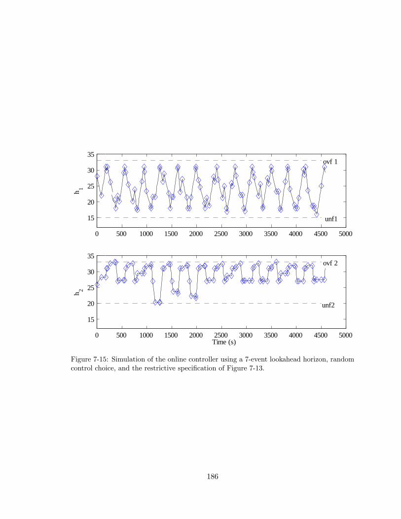
0 500 1000 1500 2000 2500 3000 3500 4000 4500 5000
15
20
25
30
35
Time (s)
h 1
ovf 1
unf1
0 500 1000 1500 2000 2500 3000 3500 4000 4500 5000
15
20
25
30
35
h 2
ovf 2
unf2
Figure 7-15: Simulation of the online controller using a 7-event lookahead horizon, randomcontrol choice, and the restrictive speci�cation of Figure 7-13.
186
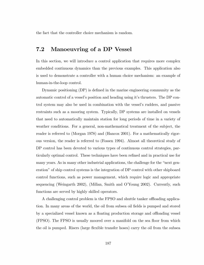
the fact that the controller choice mechanism is random.
7.2 Manoeuvring of a DP Vessel
In this section, we will introduce a control application that requires more complex
embedded continuous dynamics than the previous examples. This application also
is used to demonstrate a controller with a human choice mechanism: an example of
human-in-the-loop control.
Dynamic positioning (DP) is de�ned in the marine engineering community as the
automatic control of a vessel�s position and heading using it�s thrusters. The DP con-
trol system may also be used in combination with the vessel�s rudders, and passive
restraints such as a mooring system. Typically, DP systems are installed on vessels
that need to automatically maintain station for long periods of time in a variety of
weather conditions. For a general, non-mathematical treatment of the subject, the
reader is referred to (Morgan 1978) and (Hancox 2001). For a mathematically rigor-
ous version, the reader is referred to (Fossen 1994). Almost all theoretical study of
DP control has been devoted to various types of continuous control strategies, par-
ticularly optimal control. These techniques have been re�ned and in practical use for
many years. As in many other industrial applications, the challenge for the �next gen-
eration�of ship control systems is the integration of DP control with other shipboard
control functions, such as power management, which require logic and appropriate
sequencing (Weingarth 2002), (Millan, Smith and O�Young 2002). Currently, such
functions are served by highly skilled operators.
A challenging control problem is the FPSO and shuttle tanker o oading applica-
tion. In many areas of the world, the oil from subsea oil �elds is pumped and stored
by a specialized vessel known as a �oating production storage and o oading vessel
(FPSO). The FPSO is usually moored over a manifold on the sea �oor from which
the oil is pumped. Risers (large �exible transfer hoses) carry the oil from the subsea
187
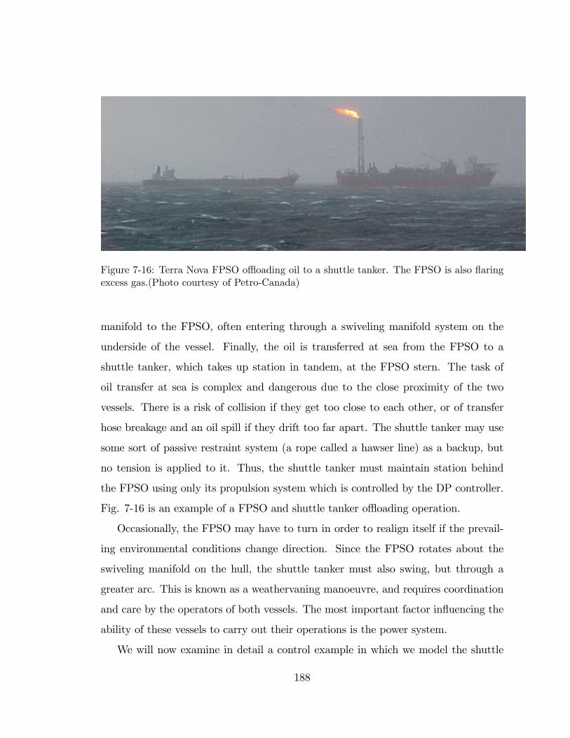
Figure 7-16: Terra Nova FPSO o oading oil to a shuttle tanker. The FPSO is also �aringexcess gas.(Photo courtesy of Petro-Canada)
manifold to the FPSO, often entering through a swiveling manifold system on the
underside of the vessel. Finally, the oil is transferred at sea from the FPSO to a
shuttle tanker, which takes up station in tandem, at the FPSO stern. The task of
oil transfer at sea is complex and dangerous due to the close proximity of the two
vessels. There is a risk of collision if they get too close to each other, or of transfer
hose breakage and an oil spill if they drift too far apart. The shuttle tanker may use
some sort of passive restraint system (a rope called a hawser line) as a backup, but
no tension is applied to it. Thus, the shuttle tanker must maintain station behind
the FPSO using only its propulsion system which is controlled by the DP controller.
Fig. 7-16 is an example of a FPSO and shuttle tanker o oading operation.
Occasionally, the FPSO may have to turn in order to realign itself if the prevail-
ing environmental conditions change direction. Since the FPSO rotates about the
swiveling manifold on the hull, the shuttle tanker must also swing, but through a
greater arc. This is known as a weathervaning manoeuvre, and requires coordination
and care by the operators of both vessels. The most important factor in�uencing the
ability of these vessels to carry out their operations is the power system.
We will now examine in detail a control example in which we model the shuttle
188
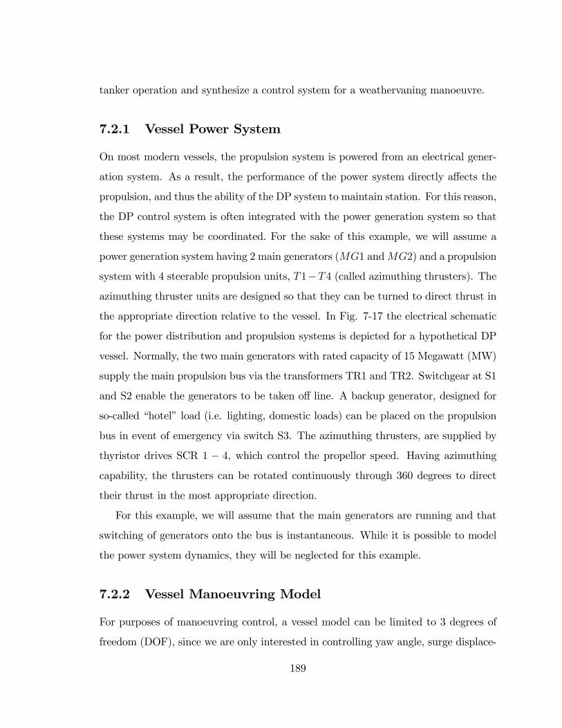
tanker operation and synthesize a control system for a weathervaning manoeuvre.
7.2.1 Vessel Power System
On most modern vessels, the propulsion system is powered from an electrical gener-
ation system. As a result, the performance of the power system directly a¤ects the
propulsion, and thus the ability of the DP system to maintain station. For this reason,
the DP control system is often integrated with the power generation system so that
these systems may be coordinated. For the sake of this example, we will assume a
power generation system having 2 main generators (MG1 andMG2) and a propulsion
system with 4 steerable propulsion units, T1�T4 (called azimuthing thrusters). The
azimuthing thruster units are designed so that they can be turned to direct thrust in
the appropriate direction relative to the vessel. In Fig. 7-17 the electrical schematic
for the power distribution and propulsion systems is depicted for a hypothetical DP
vessel. Normally, the two main generators with rated capacity of 15 Megawatt (MW)
supply the main propulsion bus via the transformers TR1 and TR2. Switchgear at S1
and S2 enable the generators to be taken o¤ line. A backup generator, designed for
so-called �hotel�load (i.e. lighting, domestic loads) can be placed on the propulsion
bus in event of emergency via switch S3. The azimuthing thrusters, are supplied by
thyristor drives SCR 1 � 4, which control the propellor speed. Having azimuthing
capability, the thrusters can be rotated continuously through 360 degrees to direct
their thrust in the most appropriate direction.
For this example, we will assume that the main generators are running and that
switching of generators onto the bus is instantaneous. While it is possible to model
the power system dynamics, they will be neglected for this example.
7.2.2 Vessel Manoeuvring Model
For purposes of manoeuvring control, a vessel model can be limited to 3 degrees of
freedom (DOF), since we are only interested in controlling yaw angle, surge displace-
189

MG1 MG2
TR1 TR2
SCR1 SCR2 SCR3 SCR4
T1 T2 T3 T4
15 MW 15 MW
4 X 7.5 MW
MG3
OtherLoads
5 MW
TR3
S1 S2S3
Figure 7-17: The power distribution and propulsion load schematic for a hypothetical vessel.
190
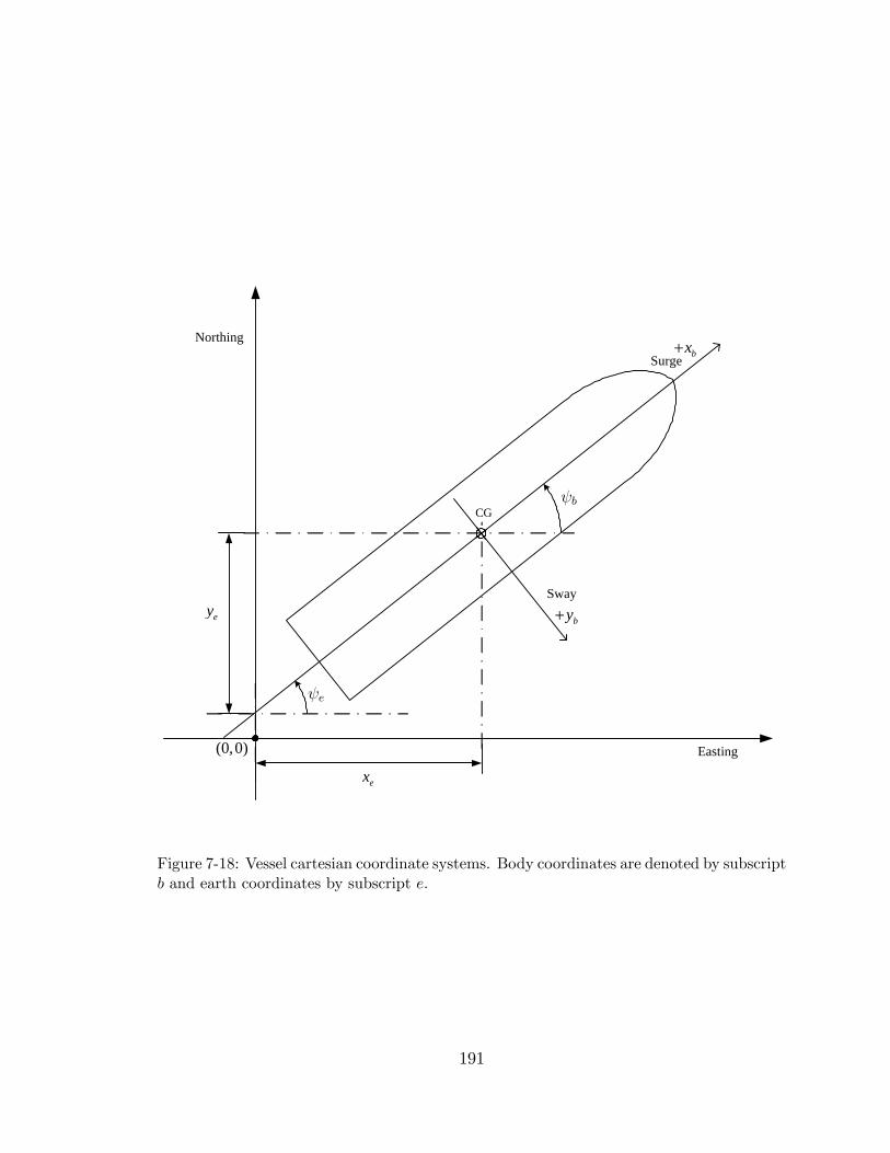
CG
Sway
Surgebx+
by+
ex
ey
Northing
Easting(0,0)
ψe
ψb
Figure 7-18: Vessel cartesian coordinate systems. Body coordinates are denoted by subscriptb and earth coordinates by subscript e.
191
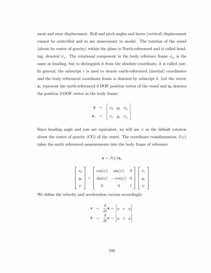
ment and sway displacement. Roll and pitch angles and heave (vertical) displacement
cannot be controlled and so are unnecessary to model. The rotation of the vessel
(about its centre of gravity) within the plane is North-referenced and is called head-
ing, denoted e. The rotational component in the body reference frame b, is the
same as heading, but to distinguish it from the absolute coordinate, it is called yaw.
In general, the subscript e is used to denote earth-referenced (inertial) coordinates
and the body referenced coordinate frame is denoted by subscript b. Let the vector
xe represent the earth-referenced 3 DOF position vector of the vessel and xb denotes
the position 3 DOF vector in the body frame:
x =hxb yb b
ixe =
hxe ye e
iSince heading angle and yaw are equivalent, we will use as the default rotation
about the center of gravity (CG) of the vessel. The coordinate transformation J( )
takes the earth referenced measurements into the body frame of reference:
x = J( )xe26664xb
yb
37775 =26664cos( ) sin( ) 0
sin( ) � cos( ) 0
0 0 1
3777526664xe
ye
37775We de�ne the velocity and acceleration vectors accordingly:
v =d
dtx =
hu v �
i_v =
d
dtv =
h_u _v _�
i
192
The simpli�ed (linear) dynamics of a freely-�oating (i.e. unmoored) surface vessel
can then be characterized by the following vector di¤erential equation:
M _v+Dv=� (7.2)
� is the force and moment vector acting upon the vessel that arises from the sum
of the control forces, � c and the environmental forces (current, waves and wind), � e,
each de�ned in the inertial frame.
� = � c + � e
M is a positive de�nite matrix (M =MT ) containing the inertial and hydrodynamic
added mass terms for the vessel as follows:
M =
26664m+X _u 0 0
0 m+ Y _v mxG + Y _r
0 mxG + Y _r Izz +N _r
37775where m is the vessel�s mass, Izz is the yaw moment of inertia, X _u, Y _v, are the
hydrodynamic added mass in the surge axis, sway axes respectively and N _r is the
added moment of inertia in the yaw axis. The o¤-diagonal terms are symmetrical
(this follows, since the vessel is symmetrical about both the surge and sway axes),
and feature a hydrodynamic added mass term Y _r due to the cross-coupling between
the sway and yaw axes. mxG is present when the vessel�s control point (CP)1 is not
the same as the center of mass (CG) of the vessel. The longitudinal distance between
CP and CG is xG is (Fig. 7-18).
1The control point is the point in the body coordinate frame which is positioned by the DPcontroller.
193
Table 7.3: The FPSO vessel particulars.Vessel Particular Full ScaleLength Overall (LOA) 290 mDisplacement, r 193,000 m3
Mass 197,632 tonnesYaw Radius of Gyration 57 mBeam 45 mLongitudinal CG 145 m
D is a matrix containing linear hydrodynamic damping terms:
D =
26664Xu 0 0
0 Yv Yr
0 Nv Nr
37775the diagonal terms Xu, Yv and Nr, are the surge sway and yaw damping. The
o¤-diagonal terms Yr and Nv are respectively, the sway-yaw and yaw-sway damping
terms.
Assumptions that have been made to simplify this model are that centripetal and
Coriolis forces are negligible because yaw rates are relatively small, and hydrody-
namic added mass and damping are constant. Since most DP vessels are designed
for stationkeeping, and vessel velocities are low, this assumption is also reasonable.
The hydrodynamic added mass and damping can be determined by specialized soft-
ware, estimated from existing ships for which these parameters are already known,
or determined empirically by model testing or full-scale ship trials. The detailed ves-
sel particulars for the vessel that will be simulated are given in Table 7.3. For the
simulation, we will use non-dimensional quantities for convenience. The so called bis
system ((Fossen 1994), p. 94) is a convenient system for low-speed manoeuvring mod-
els, since it is not based on vessel forward speed as other systems are. The bis system
non-dimensional scaling factors for a surface vessel are given in Table 7.4. Typically,
the vessel LOA is used for the length factor L, g is the acceleration due to gravity, �
194
Table 7.4: Nondimensional scaling factors.Quantity Scale FactorMass �rLength LLinear Velocity
pgL
Angular velocityp
gL
Force �grMoment �grLTime
qLg
is the density of sea water (1025 kg=m3). As an example, the non-dimensional mass
of the vessel at full displacement is m = 1.
7.2.3 Closed Loop Control
For this example, the discrete event controller will supervise a closed loop continuous
controller (i.e. the DP control system). Therefore, the switched continuous model will
be developed around CSMs that model the closed-loop dynamics of the vessel. Figure
7-19 is a block diagram of a typical DP control system. The system is commanded
with a 3 DOF setpoint command in earth referenced coordinates. The vessel�s 3
DOF position xe is measured with a variety of sensors and passed through a state
estimator2. The error signal is converted to body coordinates, and control gains
are applied to determine a controller demand. Measurements of the wind speed
and direction are used to calculate a feedforward wind load, which is summed to
the controller demand. A thruster allocation block determines how this controller
� c demand will be divided amongst the available thrusters, taking the geometry of
their hull arrangement into account. Not pictured in the �gure is the optimal state
estimation current and wave generated forces and moment; these are summed into
the controller demand.
2Typically, a Kalman �lter is used to remove sensor noise.
195
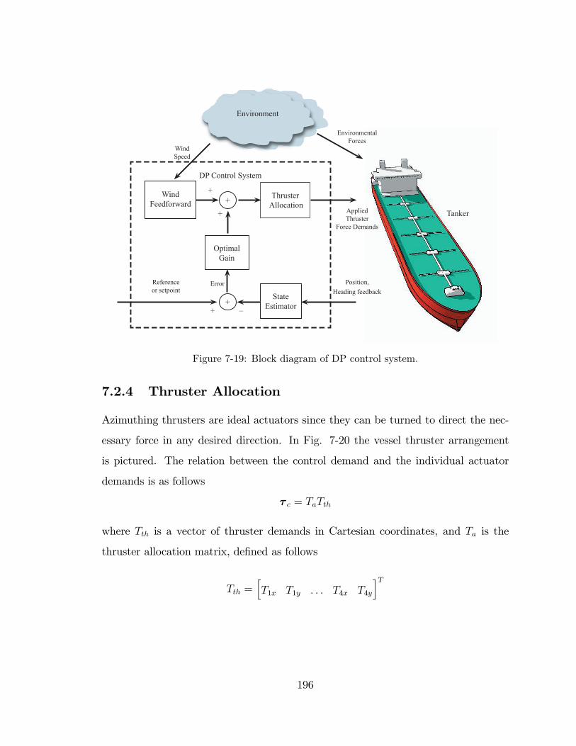
Environment
DP Control System
Thruster Allocation
OptimalGain
WindFeedforward +
StateEstimator+
EnvironmentEnvironment
Position, Heading feedback
AppliedThruster
Force Demands
Environmental Forces
ErrorReferenceor setpoint
WindSpeed
+ _
+
+ Tanker
Figure 7-19: Block diagram of DP control system.
7.2.4 Thruster Allocation
Azimuthing thrusters are ideal actuators since they can be turned to direct the nec-
essary force in any desired direction. In Fig. 7-20 the vessel thruster arrangement
is pictured. The relation between the control demand and the individual actuator
demands is as follows
� c = TaTth
where Tth is a vector of thruster demands in Cartesian coordinates, and Ta is the
thruster allocation matrix, de�ned as follows
Tth =hT1x T1y : : : T4x T4y
iT
196
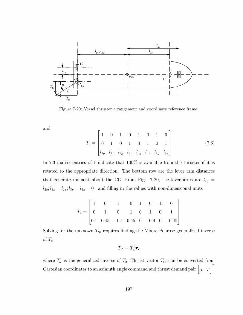
T2
T1
T3
1 2,x xl l
2 yl
3xl4 xl
1α1T
1xT
1yT
CG
Figure 7-20: Vessel thruster arrangement and coordinate reference frame.
and
Ta =
266641 0 1 0 1 0 1 0
0 1 0 1 0 1 0 1
l1y l1x l2y l2x l3y l3x l4y l4x
37775 (7.3)
In 7.3 matrix entries of 1 indicate that 100% is available from the thruster if it is
rotated to the appropriate direction. The bottom row are the lever arm distances
that generate moment about the CG. From Fig. 7-20, the lever arms are l1y =
l2y; l1x = l2x; l3y = l4y = 0 , and �lling in the values with non-dimensional units
Ta =
266641 0 1 0 1 0 1 0
0 1 0 1 0 1 0 1
0:1 0:45 �0:1 0:45 0 �0:4 0 �0:45
37775Solving for the unknown Tth requires �nding the Moore Penrose generalized inverse
of Ta
Tth = T ya� c
where T ya is the generalized inverse of Ta: Thrust vector Tth can be converted from
Cartesian coordinates to an azimuth angle command and thrust demand pairh� T
iT
197
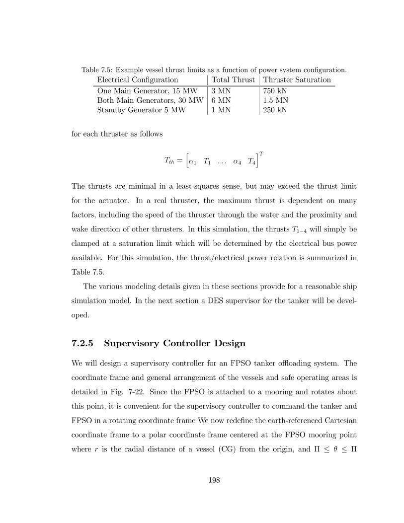
Table 7.5: Example vessel thrust limits as a function of power system con�guration.Electrical Con�guration Total Thrust Thruster SaturationOne Main Generator, 15 MW 3 MN 750 kNBoth Main Generators, 30 MW 6 MN 1.5 MNStandby Generator 5 MW 1 MN 250 kN
for each thruster as follows
Tth =h�1 T1 : : : �4 T4
iTThe thrusts are minimal in a least-squares sense, but may exceed the thrust limit
for the actuator. In a real thruster, the maximum thrust is dependent on many
factors, including the speed of the thruster through the water and the proximity and
wake direction of other thrusters. In this simulation, the thrusts T1�4 will simply be
clamped at a saturation limit which will be determined by the electrical bus power
available. For this simulation, the thrust/electrical power relation is summarized in
Table 7.5.
The various modeling details given in these sections provide for a reasonable ship
simulation model. In the next section a DES supervisor for the tanker will be devel-
oped.
7.2.5 Supervisory Controller Design
We will design a supervisory controller for an FPSO tanker o oading system. The
coordinate frame and general arrangement of the vessels and safe operating areas is
detailed in Fig. 7-22. Since the FPSO is attached to a mooring and rotates about
this point, it is convenient for the supervisory controller to command the tanker and
FPSO in a rotating coordinate frame We now rede�ne the earth-referenced Cartesian
coordinate frame to a polar coordinate frame centered at the FPSO mooring point
where r is the radial distance of a vessel (CG) from the origin, and � � � � �
198

0 100 200 300 400 500 6000
0.5
1
1.5
2
2.5
3
Time(s)
Thru
ster
Dem
and
(MN
)
T1T2T3T4Total
Figure 7-21: Individual thrusts for a step maneouver in yaw, using one generator.
199
is the angle of rotation, while is the vessel heading, unchanged from the other
coordinate frames. All ranges r in this diagram are nondimensional. The scenario
we are designing a controller for is a weathervaning manoeuvre that only the tanker
carries out. When the �are is lit on the FPSO, the forward deck temperature of the
tanker can rise to dangerous levels. the written operating procedures (Allan 1999)
require that the operator of the FPSO contact the tanker and request that it move
in order to minimize the deck heating. Since the �are is on the starboard side of the
FPSO, movement of the tanker slightly to the port side of the FPSO�s stern has the
desired e¤ect. during this move, the appropriate separation between the vessels must
still be maintained to prevent collision or hose breakage. In Fig. 7-22 the green zone
is the normal safe area in absence of a �are. The red-coloured zone is a �keep-out�
area due to subsea risers that may be damaged by the tanker�s thrusters. The blue
area to the port side of the FPSO is the safe area while the �are is operating. We
will design a controller to enforce safe operation during a �are event.
7.2.5.1 Partitions and Output Events
We begin the modeling process by de�ning the partitioning functionals for the system
SCM in Table 7.6. In this case, we use a partial state vector
x =hr � t
iNote that we are using the polar coordinate frame with origin at the mooring point
of the FPSO. Events tfp and tfs signal when the vessel longitudinal axis is out of
alignment with the coordinate frame; the goal is to keep the bow of the tanker aimed
towards the FPSO at all times3. The esd emergency shutdown is assumed to be
achieved once the vessel has safely reached a radial distance rsd � 1:85.
3Alternatively, the origin of the polar coordinate frame could be placed at the stern of the FPSO.
200

FPSO
θ
r
1.25clr =1.35nomr =
1.45fbr =
1.85sdr =Risers
Flare
Hose &Hawser
MooredPoint
1 1.4θ = −2 1.8θ = −
4 2.1θ = −
3 1.9θ = −
FlaringSafe
Tanker
PrevailingEnvironmental
Forces
Figure 7-22: The FPSO and tanker o oading system.
201
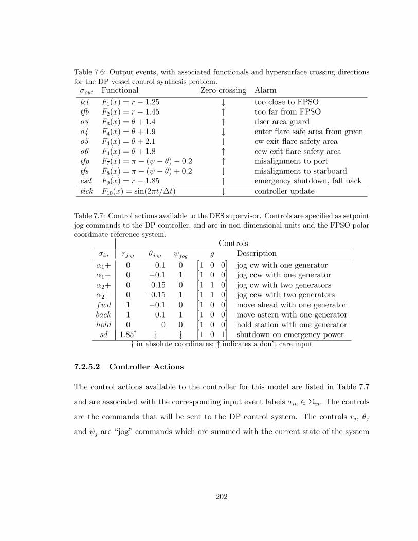
Table 7.6: Output events, with associated functionals and hypersurface crossing directionsfor the DP vessel control synthesis problem.�out Functional Zero-crossing Alarmtcl F1(x) = r � 1:25 # too close to FPSOtfb F2(x) = r � 1:45 " too far from FPSOo3 F3(x) = � + 1:4 " riser area guardo4 F4(x) = � + 1:9 # enter �are safe area from greeno5 F4(x) = � + 2:1 # cw exit �are safety areao6 F4(x) = � + 1:8 " ccw exit �are safety areatfp F7(x) = � � ( � �)� 0:2 " misalignment to porttfs F8(x) = � � ( � �) + 0:2 # misalignment to starboardesd F9(x) = r � 1:85 " emergency shutdown, fall backtick F10(x) = sin(2�t=�t) # controller update
Table 7.7: Control actions available to the DES supervisor. Controls are speci�ed as setpointjog commands to the DP controller, and are in non-dimensional units and the FPSO polarcoordinate reference system.
Controls�in rjog �jog jog g Description�1+ 0 0:1 0
�1 0 0
�jog cw with one generator
�1� 0 �0:1 1�1 0 0
�jog ccw with one generator
�2+ 0 0:15 0�1 1 0
�jog cw with two generators
�2� 0 �0:15 1�1 1 0
�jog ccw with two generators
fwd 1 �0:1 0�1 0 0
�move ahead with one generator
back 1 0:1 1�1 0 0
�move astern with one generator
hold 0 0 0�1 0 0
�hold station with one generator
sd 1:85y z z�1 0 1
�shutdown on emergency power
y in absolute coordinates; z indicates a don�t care input
7.2.5.2 Controller Actions
The control actions available to the controller for this model are listed in Table 7.7
and are associated with the corresponding input event labels �in 2 �in. The controls
are the commands that will be sent to the DP control system. The controls rj, �j
and j are �jog�commands which are summed with the current state of the system
202
to develop an absolute setpoint for the DP controller.
rsp = r + rjog
�sp = � + �jog
sp = + jog
The control indicated by g =hS1 S2 S3
i2 f0; 1g is a vector corresponding to the
generator switchgear of Fig. 7-17. Within the controller simulation, the e¤ect of this
switchgear control input is that it sets the saturation limit of the thrusters as per
Table 7.5.
7.2.5.3 Modeled Environmental Load
In heavy environmental loading, it is necessary to align a vessel with the prevailing
direction of this load in order to minimize the thruster e¤ort required to stay on
station, and in the case of the moored vessel, it reduces the vessel motion. For
our scenario, we are assuming that the FPSO is aligned with this environmental
load. When the tanker moves around to avoid the �are, it encounters a load that
progressively increases in proportion to the misalignment of the vessel with the load
vector. As the tanker moves from out of the �shadow�of the FPSO and its beam is
exposed to the waves and wind, this will tend to drag the vessel o¤ station. We will
assume that this load is a modeled e¤ect. Thus, this force is predictable and it can
be embedded in the continuous system models.
7.2.5.4 Speci�cations
For the �rst example, we will direct the vessel to rotate from its initial position, with
a heading of = �=2 and positioned directly behind the FPSO in the green zone
(Fig. 7-22). The assumption is that the FPSO has communicated to the tanker
that it will commence �aring gas so the tanker must move to the �are safe area.
203
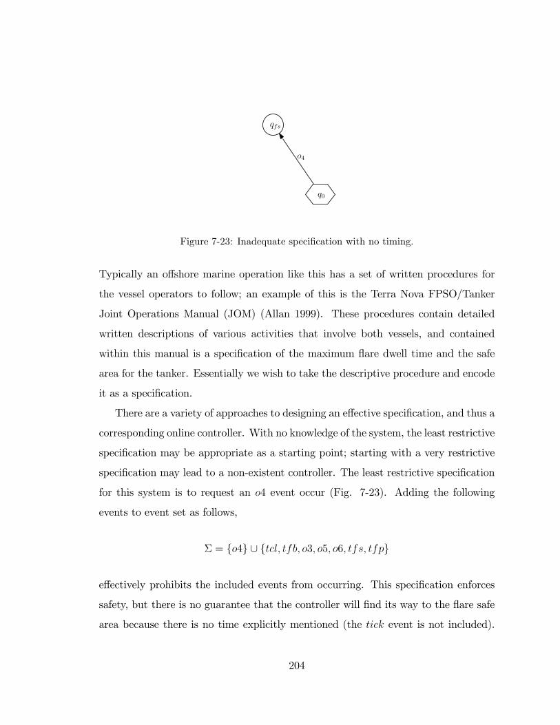
q0
qfs
o4
CG
Sway
Surgebx+
by+
ex
ey
Northing
Easting(0,0)
ψe
ψb
Figure 7-23: Inadequate speci�cation with no timing.
Typically an o¤shore marine operation like this has a set of written procedures for
the vessel operators to follow; an example of this is the Terra Nova FPSO/Tanker
Joint Operations Manual (JOM) (Allan 1999). These procedures contain detailed
written descriptions of various activities that involve both vessels, and contained
within this manual is a speci�cation of the maximum �are dwell time and the safe
area for the tanker. Essentially we wish to take the descriptive procedure and encode
it as a speci�cation.
There are a variety of approaches to designing an e¤ective speci�cation, and thus a
corresponding online controller. With no knowledge of the system, the least restrictive
speci�cation may be appropriate as a starting point; starting with a very restrictive
speci�cation may lead to a non-existent controller. The least restrictive speci�cation
for this system is to request an o4 event occur (Fig. 7-23). Adding the following
events to event set as follows,
� = fo4g [ ftcl; tfb; o3; o5; o6; tfs; tfpg
e¤ectively prohibits the included events from occurring. This speci�cation enforces
safety, but there is no guarantee that the controller will �nd its way to the �are safe
area because there is no time explicitly mentioned (the tick event is not included).
204
E¤ectively this means that the system has been commanded to reach the safe area but
nothing has been said about the timing of this activity. This speci�cation is unsuitable
since there is no upper bound on the time that the vessel can remain in the green
zone while the �are is operating. An additional problem with this speci�cation is
that the controller synthesized with this approach will have to use a low time or
event lookahead to avoid the exponential growth in controller size.
A di¤erent approach is to choose speci�cation that includes some speci�c timing
information. The designer must specify to a greater or lesser degree the time at which
the �are safe zone will be entered, since if the vessel remains too long in the vicinity
of the �are, it will violate the system safety. However, too �tight� a speci�cation
can lead to blocking and an unnecessary emergency shutdown. Too �open�a spec-
i�cation, and controller complexity may become a problem. One possible approach
is to �calibrate� the trajectory by manually running simulations o ine to test the
time required to reach safety from a variety of initial conditions. The speci�cation
can then be tailored to admit the trajectories with the �calibrated� timing. Such
�over-speci�cation� defeats the purpose of this type of online controller synthesis,
since the set of control solutions is decided o ine. This approach is shown in Fig.
7-24(b). In this speci�cation, an upper limit of 6 events has been speci�ed for the
vessel to move to the �are safe area. Some �exibility has been built in by allowing
for it to take place sooner in 5 events. Without calibration, it is possible that this
speci�cation may eliminate control trajectories that will take the vessel to the �are
safe area before this time.
The speci�cation of Fig. 7-24(b) does not specify a lower time limit for the
manoeuvre, but e¤ectively is the same as that of Fig. 7-24(a) in terms of complexity.
By not specifying the lower limit, we have made no presumption of the vessel initial
condition or dynamics. The upper bound on the speci�cation time (6 events) is
derived not from the vessel dynamics, but is based on the maximum time the vessel
can linger in the green zone while the �are is lit, which is derived directly from the
205
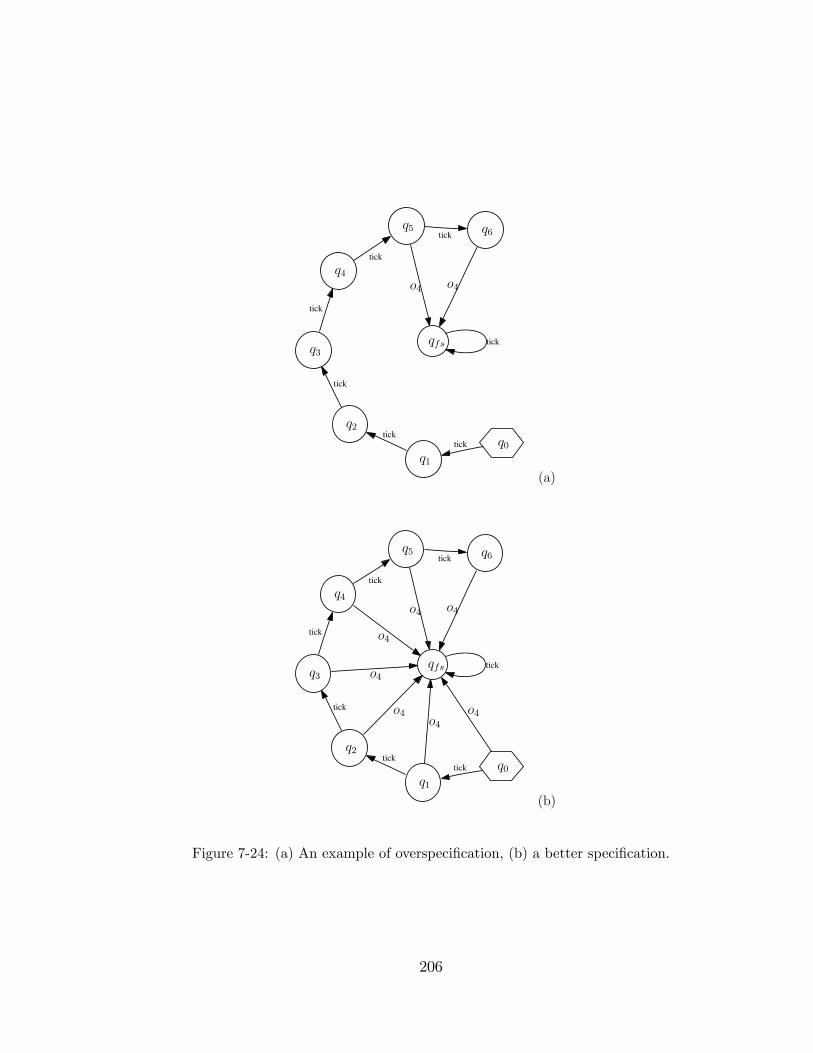
tick
tick
tick
tick
tick
tick
tick
q0
q1
q2
q3
q4
q5 q6
qfs
o4o4
(a)
tick
tick
tick
tick
tick
tick
tick
q0
q1
q2
q3
q4
q5 q6
qfs
o4o4
o4
o4
o4
o4
o4
(b)
Figure 7-24: (a) An example of overspeci�cation, (b) a better speci�cation.
206
operational procedures manual (the JOM). This will be the speci�cation used for the
controller synthesis and simulation.
7.2.6 Results
The modeling information of the preceding sections was used to develop a switched
continuous model. Using HySynth to simulate the closed-loop system, the following
test results were obtained for supervisory control of the weathervaning manoeuvre.
The tick time used for these simulations was �t = 100 (unitless).
7.2.6.1 Control With Random Choice
Running a simulation of the weathervaning manoeuvre using the speci�cations of
Fig. 7-24, generally will result in a shutdown if the event or time lookahead horizon
is not large enough to include state q6 of the speci�cation. The control synthesis
has to have large enough lookahead to perceive that state q6 is blocking if the vessel
cannot subsequently reach the �are safe area (state qfs). With an event or time
lookahead that is too short, the control system is not able to distinguish between
an output string of 5 ticks that is moving to safety from a an output string that
is simply staying within the green zone. This is clearly illustrated in Table 7.8, in
which the controller has a 5 event lookahead combined with a random control choice
mechanism. The table is read from left to right: e.g. at step 1, there are a total of
jAj = jAe + Aenj = 6 control actions available for the operator to choose amongst.
The second and third columns are the legal input event subsets, that are eligible as
control actions: recall that Ae is the set of control actions that lead only to ESD and
Aen is the set of events that lead to ESD reachable and nonblocking states.
Starting at Step 1, the controller has 5 priority 1 choices (ESD reachable and non-
blocking), so using a random choice mechanism, it actually selects a+2 which is driving
with both generators in the wrong direction. It continues to do this action in the next
step, when suddenly the speci�cation has reached a block in the lookahead; i.e. o4
207
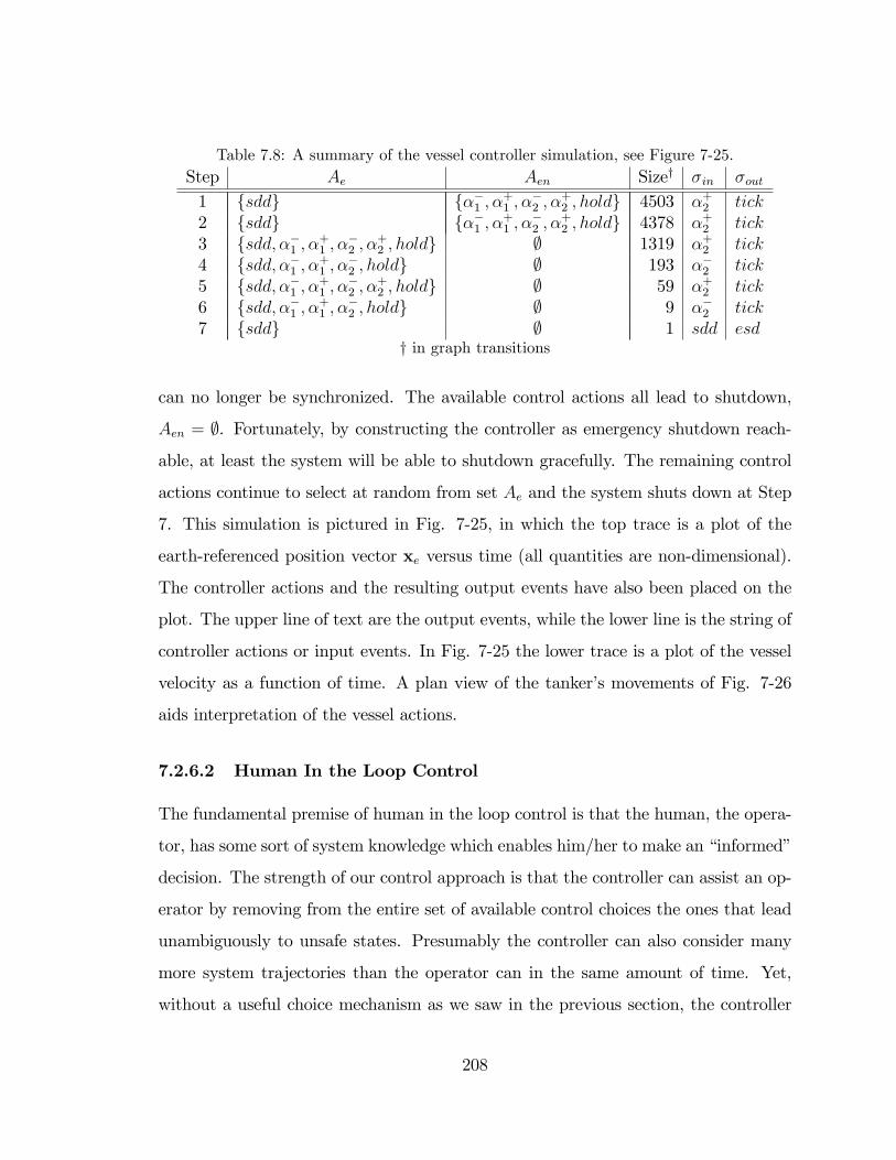
Table 7.8: A summary of the vessel controller simulation, see Figure 7-25.Step Ae Aen Sizey �in �out
1 fsddg f��1 ; �+1 ; ��2 ; �+2 ; holdg 4503 �+2 tick2 fsddg f��1 ; �+1 ; ��2 ; �+2 ; holdg 4378 �+2 tick3 fsdd; ��1 ; �+1 ; ��2 ; �+2 ; holdg ; 1319 �+2 tick4 fsdd; ��1 ; �+1 ; ��2 ; holdg ; 193 ��2 tick5 fsdd; ��1 ; �+1 ; ��2 ; �+2 ; holdg ; 59 �+2 tick6 fsdd; ��1 ; �+1 ; ��2 ; holdg ; 9 ��2 tick7 fsddg ; 1 sdd esd
y in graph transitions
can no longer be synchronized. The available control actions all lead to shutdown,
Aen = ;. Fortunately, by constructing the controller as emergency shutdown reach-
able, at least the system will be able to shutdown gracefully. The remaining control
actions continue to select at random from set Ae and the system shuts down at Step
7. This simulation is pictured in Fig. 7-25, in which the top trace is a plot of the
earth-referenced position vector xe versus time (all quantities are non-dimensional).
The controller actions and the resulting output events have also been placed on the
plot. The upper line of text are the output events, while the lower line is the string of
controller actions or input events. In Fig. 7-25 the lower trace is a plot of the vessel
velocity as a function of time. A plan view of the tanker�s movements of Fig. 7-26
aids interpretation of the vessel actions.
7.2.6.2 Human In the Loop Control
The fundamental premise of human in the loop control is that the human, the opera-
tor, has some sort of system knowledge which enables him/her to make an �informed�
decision. The strength of our control approach is that the controller can assist an op-
erator by removing from the entire set of available control choices the ones that lead
unambiguously to unsafe states. Presumably the controller can also consider many
more system trajectories than the operator can in the same amount of time. Yet,
without a useful choice mechanism as we saw in the previous section, the controller
208

0 100 200 300 400 500 600 700 800 900
1.4
1.6
1.8
2
Ves
sel P
ositi
on
α2+ tickα2+ tickα2+ tickα2 tickα2+ tickα2 ticksdd esd
0 100 200 300 400 500 600 700 800 9005
0
5
Time
Ves
sel V
eloc
ity 1
03
re
θe
ψe
uvφ
Figure 7-25: Simulation with inadequate event horizon. Using a random choice mechanism,the system goes to ESD.
209
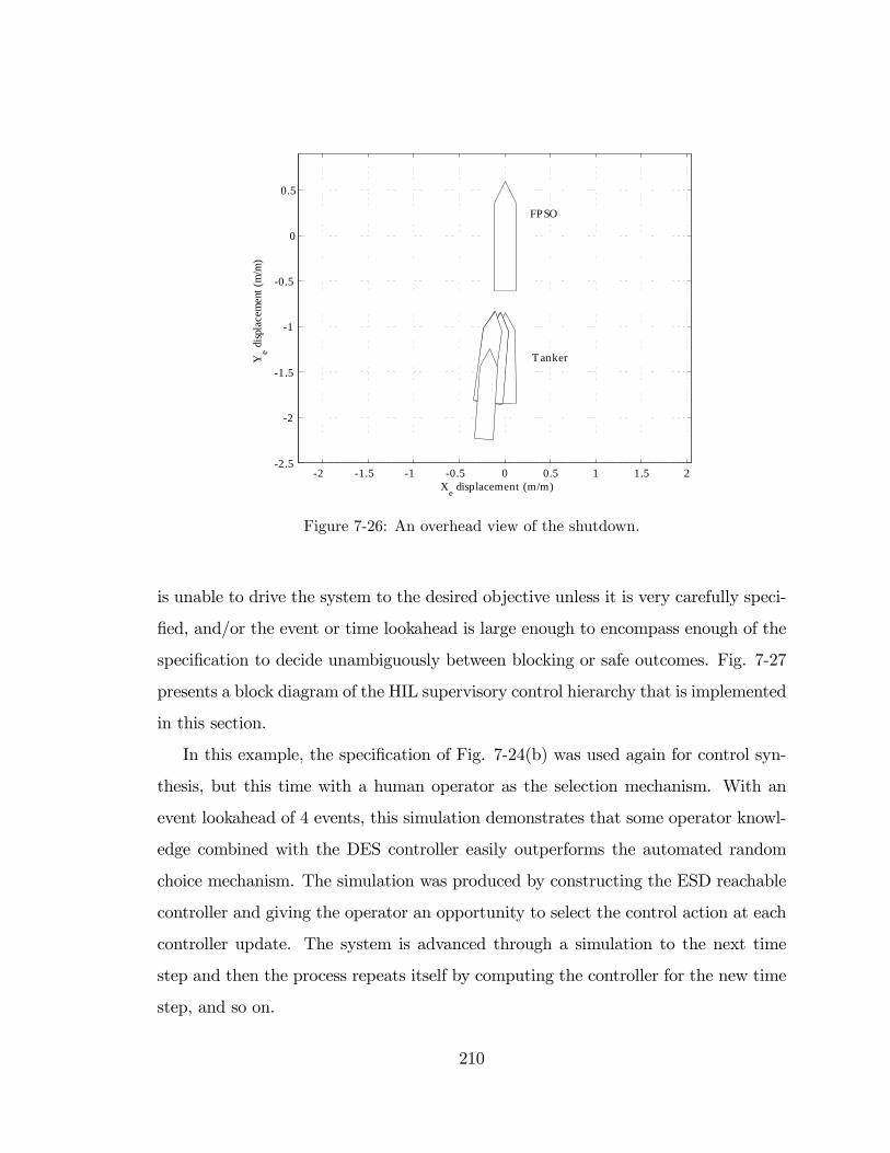
2 1.5 1 0.5 0 0.5 1 1.5 22.5
2
1.5
1
0.5
0
0.5
Xe displacement (m/m)
Ye d
ispla
cem
ent (
m/m
)
FPSO
T anker
Figure 7-26: An overhead view of the shutdown.
is unable to drive the system to the desired objective unless it is very carefully speci-
�ed, and/or the event or time lookahead is large enough to encompass enough of the
speci�cation to decide unambiguously between blocking or safe outcomes. Fig. 7-27
presents a block diagram of the HIL supervisory control hierarchy that is implemented
in this section.
In this example, the speci�cation of Fig. 7-24(b) was used again for control syn-
thesis, but this time with a human operator as the selection mechanism. With an
event lookahead of 4 events, this simulation demonstrates that some operator knowl-
edge combined with the DES controller easily outperforms the automated random
choice mechanism. The simulation was produced by constructing the ESD reachable
controller and giving the operator an opportunity to select the control action at each
controller update. The system is advanced through a simulation to the next time
step and then the process repeats itself by computing the controller for the new time
step, and so on.
210
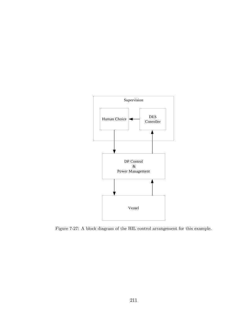
Vessel
DP Control&
Power Management
Supervision
DESConrollerHuman Choice
Figure 7-27: A block diagram of the HIL control arrangement for this example.
211
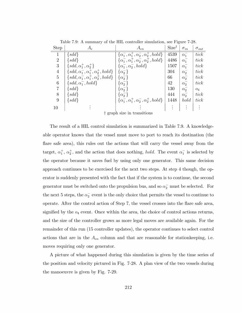
Table 7.9: A summary of the HIL controller simulation, see Figure 7-28.Step Ae Aen Sizey �in �out
1 fsddg f��1 ; �+1 ; ��2 ; �+2 ; holdg 4539 ��1 tick2 fsddg f��1 ; �+1 ; ��2 ; �+2 ; holdg 4486 ��1 tick3 fsdd; �+1 ; �+2 g f��1 ; ��2 ; holdg 1507 ��1 tick4 fsdd; ��1 ; �+1 ; �+2 ; holdg f��2 g 304 ��2 tick5 fsdd; ��1 ; �+1 ; �+2 ; holdg f��2 g 66 ��2 tick6 fsdd; ��1 ; holdg f��2 g 42 ��2 tick7 fsddg f��2 g 130 ��2 o48 fsddg f��2 g 444 ��2 tick9 fsddg f��1 ; �+1 ; ��2 ; �+2 ; holdg 1448 hold tick
10...
......
......
y graph size in transitions
The result of a HIL control simulation is summarized in Table 7.9. A knowledge-
able operator knows that the vessel must move to port to reach its destination (the
�are safe area), this rules out the actions that will carry the vessel away from the
target, �+1 , �+2 ; and the action that does nothing, hold. The event �
�1 is selected by
the operator because it saves fuel by using only one generator. This same decision
approach continues to be exercised for the next two steps. At step 4 though, the op-
erator is suddenly presented with the fact that if the system is to continue, the second
generator must be switched onto the propulsion bus, and so ��2 must be selected. For
the next 5 steps, the ��2 event is the only choice that permits the vessel to continue to
operate. After the control action of Step 7, the vessel crosses into the �are safe area,
signi�ed by the o4 event. Once within the area, the choice of control actions returns,
and the size of the controller grows as more legal moves are available again. For the
remainder of this run (15 controller updates), the operator continues to select control
actions that are in the Aen column and that are reasonable for stationkeeping, i.e.
moves requiring only one generator.
A picture of what happened during this simulation is given by the time series of
the position and velocity pictured in Fig. 7-28. A plan view of the two vessels during
the manoeuvre is given by Fig. 7-29.
212
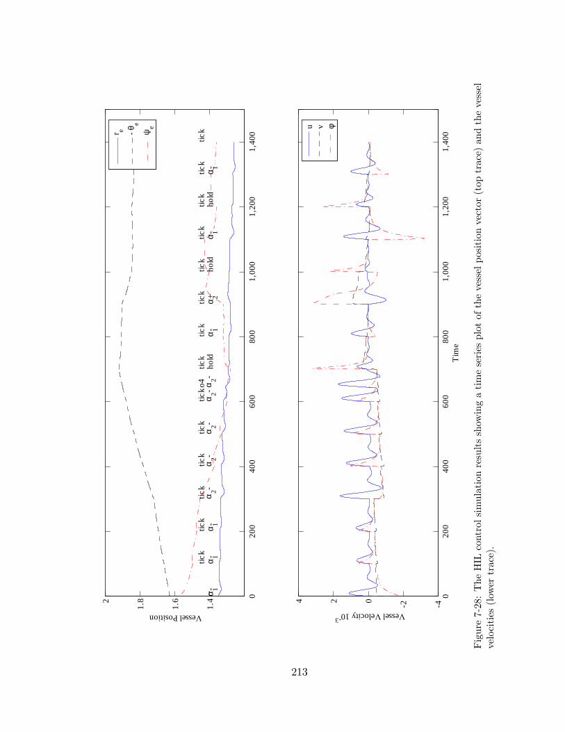
020
040
060
080
01,
000
1,20
01,
400
1.4
1.6
1.82
Vessel Position
α 1tic
kα
1tic
kα 1
tick
α2
tick
α2
tick
α2
tick
α2o4 α
2tic
kho
ldtic
kα 1
tick
α 2+tic
kho
ldtic
kα 1
tick
hold
tick
α 1tic
k
020
040
060
080
01,
000
1,20
01,
400
42024
Tim
e
Vessel Velocity 103r e θ
eψ
e u v φ
Figure7-28:TheHILcontrolsimulationresultsshowingatimeseriesplotofthevesselpositionvector(toptrace)andthevessel
velocities(lowertrace).
213
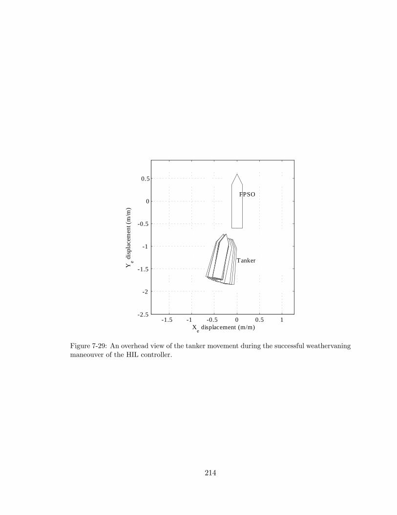
1.5 1 0.5 0 0.5 12.5
2
1.5
1
0.5
0
0.5
Xe displacement (m/m)
Ye d
ispl
acem
ent (
m/m
)
FPSO
Tanker
Figure 7-29: An overhead view of the tanker movement during the successful weathervaningmaneouver of the HIL controller.
214
7.3 Remarks
The continuous system model of Chapter 3 was proposed as the basis for modeling
the continuous dynamics of a hybrid system. Formally, the CSM accommodates
systems whose dynamics can be modeled by nonlinear ODEs. The only constraint
placed on these functions is that they be Lipschitz-continuous, in order to ensure
�nite discrete abstractions, but this is a theoretical consideration. The numerical
solution of ODEs is well understood, but as any numerical solution is simply an
approximation of the theoretical system model, there has to be a �leap of faith�; i.e.
since there is theoretically a solution to an ODE, then the numerical solver must �nd
an approximation of the solution that is su¢ cient for our purposes. Some of the issues
of course are:
� Will the solver terminate?,
� What type of solver should be used?; i.e. one must choose appropriate sti¤ness,
solver tolerance, etc.
� Will the solver locate the events?
So clearly, even ODE solvers have limitations that make the fundamental jump
from theory to implementation uncertain.
Given that there will be implementation-speci�c issues with our control framework
implementation, this implies that the theory should be used as a guide only. While
nonlinear ODEs may be appropriate for modeling many types of continuous systems,
is it possible that our computing framework may accommodate a broader range of
continuous simulation tools?
In many industries, application-speci�c simulation tools already exist; if control
system designers are to be convinced to use a hybrid control design package, they
will not be willing to alter their simulation tools to match the problem. Within our
215

framework, it may be possible to encapsulate existing simulation tools, provided they
meet some qualitative, but not theoretically rigorous conditions.
Starting with the assumption that there exists a continuous simulation tool that,
given an initial condition and some parameters, produces a numerical solution for a
particular system model. Then, we wish to specify the conditions that this simulation
is comparable to a system of ODEs an numerical ODE solver. A simulation tool, when
given a set of parameters:
1. must always produce an output (solution existence),
2. must be repeatable for the same parameters (solution uniqueness)
3. the solution can be computed in less time than it takes the actual system to
execute (real-time implementation).
Whether the latter requirement (3) is met, hinges primarily on the complexity of
the simulation and the extent to which the speci�cation limits the legal trajectories
of the plant. The computational hardware including the installed memory and CPU
power may also in�uence (3) to a lesser extent.
If a simulation tool meets each of the above requirements, then with suitable
wrapper functions (object methods), an SCM can be built around it, and an online
hybrid controller is feasible.
We have demonstrated in the vessel control example of §7.2, that a complex con-
tinuous simulation may be embedded seamlessly into the SCM framework and the
online controller synthesis works as expected. This vessel simulation appears to con-
form to practical requirements 1 and 2 above, and may even meet requirement 3 given
a choice of appropriate lookahead horizon, control choice mechanism and CPU power.
For this size of vessel, the actual controller update time �t is
�t =
sL
g� 100 = 538 seconds
216
Given the current state of computing hardware, it is conceivable that such a controller
update time is more than adequate to implement this controller in real time. Clearly
this would be the subject of future work.
7.4 Summary
This chapter has demonstrated the utility of the switched continuous modeling frame-
work as a basis for simulation and control synthesis for hybrid systems. The theoreti-
cal results of the preceding chapters have been con�rmed, particularly those regarding
controller complexity and guaranteed controller safety. Some of the issues that have
been dealt with in this chapter are: the process of developing a SCM, the encapsu-
lation of the continuous variable models, the selection of appropriate speci�cations,
and the e¤ect of control choice mechanism on the system safety. The concept of the
controller being able to maintain safety in the limited lookahead environment has
been demonstrated through emergency shutdown examples.
The vessel control application involving human in the loop control points to the
e¢ cacy of combining a very simple heuristic in the control choice mechanism with
the �brute force� of the exhaustive state-space search to yield better nonblocking
controller behaviour despite the limited lookahead horizon. Furthermore, the heuristic
might also be exploited to guide the search of the state space, thereby reducing the
computational burden.
217
Chapter8Conclusions and Future Work
8.1 Contributions
This thesis develops four main themes with respect to hybrid system control:
modeling, controller synthesis, computation and application. We will now high-
light the contributions in each of these areas.
8.1.1 Model
The SCM model (Chapter 4) is designed for the automated synthesis of discrete
event supervisory control systems. This model admits switching of continuous system
dynamics in both a time and state-dependent fashion and retains the full generality
of nonlinear continuous model dynamics. This is a signi�cant advantage over most
other hybrid synthesis and veri�cation techniques that require the hybrid system
models to use simpli�ed continuous dynamics. The SCM also admits the inclusion
of generalized simulations, enabling system designers to leverage existing numerical
simulation tools, by embedding them in the SCM.
218
8.1.2 Control Synthesis
With the online controller, prior to each control decision, a hybrid transition graph
is constructed based on a prediction of the discretized continuous dynamics for each
eligible continuous system model in synchronism with other DES plant and speci�ca-
tion processes. This graph is safe by design, because the safety speci�cation was used
to construct the graph. This graph is further pruned to eliminate blocking traces;
i.e. those that do not carry the system to the horizon. By inclusion of emergency
shutdown states, we guarantee safe operation by ensuring that these ESD states are
always reachable within the controller graph�s limited horizon; this is the fail-safe
controller.
8.1.3 Computation
The computation model is central to the controller implementation. Due to the in-
�nite state space of the hybrid model, limited lookahead horizon and �nite control
set are built-in limitations of the model. In order to extend the model through time
(into an in�nite time horizon) the controller is recomputed by incrementally extending
the lookahead horizon in a moving horizon scheme. Since this task must be imple-
mented online, an e¢ cient means of model storage and computation are necessary.
We describe an object-oriented modeling scheme that allows for compact storage of
the plant and speci�cation models; the hierarchical model storage avoids the state
explosion that normally results from ��attening� the system model. Furthermore,
the controller graph is easily constructed from the hierarchical model using a lazy
technique that helps to reduce the intermediate size of the graph reachable set. The
controller size complexity is bounded above by an expression that is exponential in
lookahead horizon, which implies that the synthesis algorithm is, for the worst-case,
exponential. However, the lower bound expression is linear in lookahead horizon,
implying that the computation may not always be intractably large. The controller
size is a function of the model state and time and the �tightness�of the speci�cation.
219
A heavily speci�ed system helps to reduce the controller size. The trade-o¤ is that
overspeci�cation can lead to controller blocking.
8.1.4 Application
Application examples (Chapter 7) demonstrate the �exibility of the modeling scheme
and provide empirical results for a reasonably complex industrial control problem.
The ship control example demonstrates failsafe embedded simulations, controller syn-
thesis, online control and HIL control, all novel concepts that have not been used in
this application before.
8.2 Future Work
Future work will focus on the areas of modeling , control synthesis, applications, and
improvements to the computational engine. Naturally, the impact of work in each of
these areas is interconnected, so they will be carried out in parallel.
In the area of modeling, the objective will be to add the ability of our SCM/CSM
modeling scheme to explicitly incorporate unmodeled continuous disturbance. Cur-
rently, the model accommodates modeled disturbance by simply including the distur-
bance model with each of the switched continuous system models. Various possible
approaches exist, including exploiting the results of robust control for performance
and stability guarantees or Monte Carlo simulation techniques.
It will be useful to develop other results around control choice mechanisms of var-
ious kinds. For example, HIL control appears to o¤er an improvement in controller
performance or optimality, something that is not addressed well by the DES supervi-
sory controller theory. HIL may not be suitable for every application, so automated
control choice mechanisms must also be studied.
From the applications standpoint, it is desirable to apply the control technique
to some of the more complex benchmark hybrid control problems, in order to pro-
220
vide further comparison of this technique to others. The ship control problem will
continue to be actively studied, by looking at power system and thruster con�gura-
tion robustness and multi-vessel coordination. A future model test may be planned
to prove the controller in a real-time control environment. Future applications will
also involve supervision and coordination of unmanned aerial vehicles (UAV) and
autonomous underwater vehicles (AUV), as these are both funded research projects
currently being carried out by the National Research Council. In both cases, there is
access to physical modeling and numerical simulation capabilities, in addition to the
underwater vehicles and aircraft. Both of these applications focus on the coordination
of multiple agents. Studying these problems from an application perspective will help
to focus future improvements to the modeling and control techniques.
Going hand in hand with improvements to modeling and applications, is the need
for further development of the computational tool HySynth. Essentially, the soft-
ware must be taken in two directions: 1) design time tool and 2) a run time tool. At
present HySynth is a proof-of-concept code. It should be further expanded as the
design-time tool; existing hybrid and DES libraries may prove to be useful extensions
to HySynth. The goal will be to create an easy-to-use design environment. The sec-
ond aspect of the software development e¤ort should be focussed towards a run-time
implementation that is optimized for the real-time online control environment. This
involves such considerations as real-time operating system (OS) selection, hardware
platform and the software development environment.
221
References
Abdelwahed, S., Su, R. and Neema, S.: 2005, A feasible lookahead control for systems
with �nite control set, Proceedings of the 2005 IEEE Conference on Control
Applications, IEEE, pp. 663�668.
Allan, H.: 1999, Joint operations manual - FPSO and shuttle tanker, Technical Report
TN-PE-OP04-X00-001, Terra Nova Petro-Canada.
Alur, R., Courcoubetis, C. and Dill, D. L.: 1993, Model-checking in dense real-time,
Information and Computation 104(1), 2�34.
Alur, R., Dang, T., Esposito, J., Hur, Y., Ivancic, F., Kumar, V., Lee, I., Mishra,
P., Pappas, G. and Sokolsky, O.: 2003, Hierarchical modeling and analysis of
embedded systems, Proceedings of the IEEE 91(1), 11�28.
Alur, R. and Dill, D. L.: 1994, A theory of timed automata, Theoretical Computer
Science 126(2), 183�235.
Balas, G. J. and Packard, A. K.: 1996, The structured singular value �-framework,
CRC Press, pp. 671�688.
Balluchi, A., Benvenuti, L. and Sangiovanni-Vincentelli, A.: 2005, Hybrid systems
in automotive electronics design, Proceedings of the 44th IEEE Conference on
Decision and Control, pp. 5618�5623.
222
Balluchi, A., Natale, F. D., Sangiovanni-Vincentelli, A. L. and van Schuppen, J. H.:
2004, Synthesis for idle speed control of an automotive engine, in R. Alur and
G. J. Pappas (eds), Proceedings of Hybrid Systems: Computation and Con-
trol(HSCC04), 7th International Workshop, Vol. 2993 of Lecture Notes in Com-
puter Science, Springer, pp. 80�94.
Bayen, A. and Tomlin, C.: 2003, Real time discrete control law synthesis for hybrid
systems using MILP: application to congested airspace, Proceedings of the 2003
American Control Conference, pp. 4620�4626.
Bemporad, A., Heemels, W. and de Schutter, B.: 2002, On hybrid systems and closed-
loop MPC systems, IEEE Transactions on Automatic Control 47(5), 863�869.
Bengtsson, J., Larsen, K. G., Larsson, F., Pettersson, P. and Yi, W.: 1995, UPPAAL
- a tool suite for automatic veri�cation of real-time systems, Hybrid Systems,
pp. 232�243.
Bernstein, D. S.: 2002, Feedback control: an invisible thread in the history of tech-
nology, IEEE Control Systems Magazine 22(2), 53�68.
Blondel, V. D. and Tsitsiklis, J. N.: 2000, A survey of computational complexity
results in systems and control, Automatica 36(9), 1249�1274.
Blondel, V. and Tsitsiklis, J.: 1999, Complexity of stability and controllability of
elementary hybrid systems, Automatica 35(3), 479�489.
Boel, R., Cao, X.-R., Cohen, G., Giua, A., Wonham, W. M. and van Schuppen, J. H.:
2002, Unity in diversity, diversity in unity: Retorspective and prospective views
on control of discrete event systems, Discrete Event Dynamic Systems: Theory
and Applications 12, 253�264.
223
Bourdon, S. E., Lawford, M. and Wonham, W. M.: 2005, Robust nonblocking su-
pervisory control of discrete-event systems, IEEE Transactions on Automatic
Control 50(12), 2015�2021.
Bozga, M., Daws, C., Maler, O., Olivero, A., Tripakis, S. and Yovine, S.: 1998,
KRONOS: A model-checking tool for real-time systems, in A. J. Hu and M. Y.
Vardi (eds), Proc. 10th International Conference on Computer Aided Veri�ca-
tion, Vancouver, Canada, Vol. 1427, Springer-Verlag, pp. 546�550.
Braatz, R. D., Young, P. M., Doyle, J. C. and Morari, M.: 1994, Computational com-
plexity of � calculation, IEEE Transactions on Automatic Control 39(5), 1000�
1002.
Brandin, B. A. and Wonham, W.: 1992, The supervisory control of timed discrete
event systems, Proceedings of the 31st IEEE Conference on Decision and Control,
pp. 3357�3362.
Branicky, M.: 1998, Multiple lyapunov functions and other analysis tools for switched
and hybrid systems, IEEE Transactions on Automatic Control 43, 475�482.
Brave, Y. and Heymann, M.: 1991, Control of discrete event systems modeled as hi-
erarchical state machines, Proceedings of the 30th IEEE Conference on Decision
and Control, pp. 1499�1504.
Brooks, C., Cataldo, A., Lee, E. A., Liu, J., Liu, X., Neuendor¤er, S. and Zheng,
H.: 2005, Hyvisual: A hybrid system visual modeler, Technical Memorandum
UCB/ERL M05/ 24, University of California, Berkeley, CA 94720.
Carloni, L., DiBenedetto, M., Pinto, A. and Sangiovanni-Vincentelli, A.: 2004, Mod-
eling techniques, programming languages, and design toolsets for hybrid systems,
Technical Report IST-2001-38314, Columbus Project.
224
Cassandras, C. G. and Lafortune, S.: 1999, Introduction to Discrete Event Systems,
Kluwer Academic Publishers.
Chung, S., Lafortune, S. and Lin, F.: 1992, Limited lookahead policies in supervi-
sory control of discrete event systems, IEEE Transactions on Automatic Control
37(12), 1921�1935.
Chung, S., Lafortune, S. and Lin, F.: 1994, Supervisory control using variable
lookahead policies, Discrete Event Dynamic System: Theory and Applications
4(3), 237�268.
Chutinan, A. and Krogh, B. H.: 2003, Computational techniques for hybrid system
veri�cation, IEEE Transactions on Automatic Control 48(1), 64�75.
Coleri, S., Ergen, M. and Koo, T.: 2002, Lifetime analysis of a sensor network with
hybrid automata modeling.
David, A. and Yi, W.: 2000, Modelling and analysis of a commercial �eld bus protocol,
Proceedings of the 12th Euromicro Conference on Real Time Systems, IEEE
Computer Society, pp. 165�172.
Daws, C., Kwiatkowska, M. Z. and Norman, G.: 2004, Automatic veri�cation of the
IEEE 1394 root contention protocol with KRONOS and PRISM, International
Journal on Software Tools for Technology Transfer (STTT), Vol. 5, pp. 221�236.
Ecker, J. and Malmborg, J.: 1999, Design and implementation of a hybrid control
strategy, IEEE Control Systems Magazine 19(4), 12�21.
Esposito, J., Kumar, V. and Pappas, G.: 2003, Multi-agent hybrid system simula-
tion, Proceedings of the 40th IEEE Conference on Decision and Control, IEEE,
pp. 780�785.
Fehnker, A., Vaandrager, F. and Zhang, M.: 2003, Modeling and verifying a Lego car
using hybrid I/O automata.
225
Fossen, T.: 1994, Guidance and Control of Ocean Vehicles, John Wiley & Sons.
Francis, B., Henton, J. W. and Zames, G.: 1984, H1-optimal feedback controllers
for linear multivariable systems, IEEE Transactions on Automatic Control AC-
29(10), 888�900.
Gansner, E., Kousto�os, E. and North, S.: 2002, Drawing Graphs with Dot, AT&T.
Gaudin, B. and Marchand, H.: 2005, Safety control of hierarchical synchronous dis-
crete event systems: A state-based approach, Proceedings of the 13th Mediter-
ranean Conference on Control and Automation, pp. 889�895.
Giorgetti, N., Pappas, G. J. and Bemporad, A.: 2005, Bounded model checking of
hybrid dynamical systems, Proceedings of the 44th IEEE Conference on Decision
and Control, pp. 672�677.
Gohari, P. and Wonham, M.: 2000, On the complexity of supervisory control design
in the RW framework, IEEE Transactions on Systems, Man, and Cybernetics
30(5), 643�652.
Grewal, M. and Andrews, A.: 1993, Kalman Filtering Theory and Practice, Prentice
Hall.
Hadj-Alouane, N., Lafortune, S. and Lin, F.: 1994, Variable lookahead supervi-
sory control with state information, IEEE Transactions on Automatic Control
39(12), 2398�2410.
Hancox, M.: 2001, Towing, Positioning and Hook-Up for O¤shore Production, Vol. 8,
Oil�eld Publications Limited.
Harel, D.: 1987, Statecharts: A visual formalism for complex systems, Science of
Computer Programming 8(3), 231�274.
226
Heemels, W., de Schutter, B. and Bemporad, A.: 2001, On the equivalence of classes of
hybrid dynamical models, Proceedings of the 40th IEEE Conference on Decision
and Control 1, 364�369.
Henzinger, T. A.: 2000, The theory of hybrid automata, Veri�cation of Digital and
Hybrid Systems 170, 265�292.
Henzinger, T. A. and Ho, P.: 1995, Algorithmic analysis of nonlinear hybrid systems,
in P. Wolper (ed.), Proceedings of the 7th International Conference On Computer
Aided Veri�cation, Vol. 939, Springer Verlag, Liege, Belgium, pp. 225�238.
Henzinger, T. A., Ho, P. and Wong-Toi, H.: 1996, A User Guide to HYTECH.
Henzinger, T. A., Ho, P. and Wong-Toi, H.: 1997, HyTech: A model checker for
hybrid systems, Software Tools for Technology Transfer 1, 110�122.
Henzinger, T. A., Kopke, P. W., Puri, A. and Varaiya, P.: 1998, What�s decidable
about hybrid automata?, Journal of Computer and System Sciences .
Henzinger, T. A. and Wong-Toi, H.: 1995a, Linear phase-portrait approximations for
nonlinear hybrid systems, Hybrid Systems, pp. 377�388.
Henzinger, T. A. and Wong-Toi, H.: 1995b, Using hytech to synthesize control para-
meters for a steam boiler, Formal Methods for Industrial Applications, pp. 265�
282.
Hespanha, J. and Morse, A.: 2002, Switching between stabilizing controllers, Auto-
matica 38(11), 1905�1917.
Hespanha, J. P.: 2004, Control Systems, Robotics, and Automation, Encyclopedia of
life support systems, Eolss Publishers Co. Ltd., Oxford, chapter Stabilization
through Hybrid Systems.
227
Heymann, M., Lin, F., Meyer, G. and Resmerita, S.: 2002, Analysis of zeno behav-
iours in hybrid systems, Proceedings of the 41st IEEE Conference on Decision
and Control, pp. 2379�2384.
Johansson, K. H., Egerstedt, M., Lygeros, J. and Sastry, S.: 1999, On the regular-
ization of zeno hybrid automata, Systems & Control Letters, Vol. 38, Elsevier,
pp. 141�150.
Kalman, R. E.: 1960, A new approach to linear �ltering and prediction problems,
Transactions of the ASME�Journal of Basic Engineering 82(Series D), 35�45.
Kaynak, O., Erbatur, K. and Ertugrul, M.: 2001, The fusion of computationally
intelligent methdologies and sliding mode control - a survey, IEEE Transactions
on Industrial Electronics 48(1), 4�17.
Khalil, H. K.: 2002, Nonlinear Systems, third edn, Prentice Hall.
Knopp, K.: 1956, In�nite Sequences and Series, Dover.
Koutsoukos, X. and Antsaklis, P.: 2001, Hierarchical control of piecewise linear hybrid
dynamical systems based on discrete abstractions, Technical Report ISIS-2001-
001, ISIS Group, University of Notre Dame.
Koutsoukos, X., Antsaklis, P., Stiver, J. and Lemmon, M.: 2000, Supervisory control
of hybrid systems, Proceedings of the IEEE, IEEE, pp. 1026�1048.
Kumar, R., Chung, H. M. and Marcus, S. I.: 1998, Extension based limited lookahead
supervision of discrete event systems, Automatica 34(11), 1327�1344.
Kumar, R. and Garg, V. K.: 1995, Modeling and Control of Logical Discrete Event
Systems, Kluwer Academic Publishers.
Lee, E. A.: 2003, Overview of the Ptolemy project, Technical Memorandum
UCB/ERL M03/25, University of California, Berkeley, CA, 94720, USA.
228
Leith, D. and Leithead, W.: 2000, Survey of gain scheduling analysis & design,
International Journal of Control 73(11), 1001�1025.
Lemmon, M. D., He, K. X. and Markovsky, I.: 1999, Supervisory hybrid systems,
IEEE Control Systems pp. 42�55.
Liberzon, D.: 2003, Switching in Systems and Control, Systems and Control: Foun-
dations and Applications, Birkhauser, Boston, MA.
Lin, F. and Wonham, M.: 1988, On observability of discrete-event systems, Informa-
tion Sciences 44, 173�198.
Lin, H. and Antsaklis, P.: 2005, Stability and stabilizability of switched linear systems:
A short survey of recent results, Proceedings of the 2005 IEEE International
Symposium on Intelligent Control, pp. 24�29.
Lynch, N., Segala, R. and Vaandrager, F.: 2003, Hybrid I/O automata, Technical
Report MIT-LCS-TR-827d, MIT Laboratory for Computer Science, Cambridge,
MA 02139.
MATLAB Programming: 2006, The MathWorks, Inc., 3 Apple Hill Drive, Natick,
MA 01760-2098.
Meder, C.: 1997, TTCT User Manual V0.5.0, Systems Control Group, University of
Toronto.
Michel, A. N.: 1996, Stability: the common thread in the evolution of feedback
control, IEEE Control Systems Magazine 16(3), 50�60.
Millan, J. and O�Young, S.: 2000, Hybrid modeling of tandem dynamically positioned
vessels, Proceedings of the 39th IEEE Conference on Decision and Control.
Millan, J. and O�Young, S.: 2006a, Hybrid system control using an online discrete
event supervisory strategy, IFAC Conference on Analysis and Design of Hybrid
Systems, IFAC.
229
Millan, J. and O�Young, S.: 2006b, On-line supervisory control of hybrid systems
using embedded simulations, Proceedings of the 8th International Workshop on
Discrete Event Systems WODES06.
Millan, J., Smith, L. and O�Young, S.: 2002, Coordination of FPSO and tanker
o oading operations, Proceedings of the MTS Dynamic Positioning Conference
2002.
Mitra, S., Wang, Y., Lynch, N. and Feron, E.: 2003, Application of hybrid I/O
automata in safety veri�cation of pitch controller for model helicopter system,
Technical Report MIT-LCS-TR-880, MIT Lab for Computer Science, Cambridge,
MA 02139.
Moor, T., Raisch, J. and Davoren, J.: 2001, Computational advantages of a two-
level hybrid control architecture, Proceedings of the 40th IEEE Conference on
Decision and Control, pp. 358�363.
Morgan, M.: 1978, Dynamic Positioning of O¤shore Vessels, PPC Books, Division of
Petroleum Publishing Company.
Mosterman, P. J.: 2002, HYBRSIM - a modeling and simulation environment for
hybrid bond graphs, Journal of Systems and Control Engineering 216, 35�46.
Oden, J. T.: 1979, Applied Funcitonal Analysis, Prentice Hall.
O�Young, S.: 1991, On the synthesis of the supervisors for timed discrete event
processes, Technical Report 9107, Department of Electrical and Computer Engi-
neering, University of Toronto.
O�Young, S. D.: 1992, Systems control group report, Object TCT: Users guide, Tech-
nical report, Department of Electrical Engineering, University of Toronto.
Palm III, W. J.: 2000, Modeling, Analysis, and Control of Dynamic Systems, second
edn, John Wiley & Sons.
230
Potocnik, B., Bemporad, A., Torrisi, F., Music, G. and Zupancic, B.: 2004, Hybrid
modelling and optimal control of a multiproduct batch plant, Control Engineer-
ing Practice 12(9), 1127�1137.
Raisch, J.: 2000, Discrete abstractions - an Input/Output point of view,Mathematical
and Computer Modeling of Dynamical Systems 6(1), 6�29. Special Issue on
Discrete Event Models of Continuous Systems.
Raisch, J. and O�Young, S.: 1998, Discrete approximation and supervisory control of
continuous systems, IEEE Transactions on Automatic Control 43(4), 569�573.
Ramadge, P. and Wonham, W.: 1987, Supervisory control of a class of discrete event
processes, SIAM Journal on Control Optimization 25(1), 206�230.
Ramadge, P. and Wonham, W.: 1989, The conrol of discrete event systems, Proceed-
ings of the IEEE 77(1), 81�98.
Rodger, S. H. and Finley, T. W.: 2006, JFLAP: An Interactive Formal Languages
and Automata Package, Jones & Bartlett Publishers.
Rudie, K. and Wonham, M.: 1992, Think globally, act locally: Decentralized super-
visory control, IEEE Transactions on Automatic Control 37(11), 1692�1708.
Shampine, L. and Gladwell, I.: 1991, Reliable solution of special event location prob-
lems for odess, ACM Transactions on Mathematical Software 17(1), 11�25.
Shampine, L. and Thompson, S.: 2000, Event location for ordinary di¤erential equa-
tions, Computers and Mathematics with Applications 39, 43�54.
Skogestad, S. and Postelthwaite, I.: 1993, Multivariable Feedback Control Analysis
and Design, Wiley.
Smith, R. and Doyle, J.: 1988, The two tank experiment: A benchmark control
problem, Proceedings of the IEEE American Control Conference 3, 403�415.
231
Stiver, J. A., Koutsoukos, X. D. and Antsaklis, P. J.: 2000, An invariant-based
approach to the design of hybrid control systems, Technical Report ISIS-2000-
001, ISIS Group, University of Notre Dame.
Stursberg, O.: 2004, A graph search algorithm for optimal control of hybrid systems,
Proceedings of the 43rd IEEE Conference on Decision and Control, pp. 1412�
1417.
Stursberg, O., Fehnker, A., Han, Z. and Krogh, B. H.: 2003, Speci�cation-guided
analysis of hybrid systems using a hierarchy of validation methods, IFAC Con-
ference on Analysis and Design of Hybrid Systems, IFAC.
Stursberg, O., Kowalewski, S., Ho¤mann, I. and Preusig, J.: 1997, Comparing timed
and hybrid automata as approximations of continuous systems, Hybrid Systems
IV, LNCS 1273, Springer-Verlag, pp. 361�377.
Su, R., Abdelwahed, S., Karsai, G. and Biswas, G.: 2003, Discrete abstraction and
supervisory control for switching systems, IEEE International Conference on
Systems, Man, and Cybernetics, Vol. 1, IEEE, pp. 415�421.
T. Stauner, O. Mueller and M. Fuchs: 1997, Using HYTECH to verify an automo-
tive control system, in O. Maler (ed.), Hybrid and Real-Time Systems, Springer
Verlag, LNCS 1201, Grenoble, France, pp. 139�153.
Thevenon, L. and Flaus, J.-M.: 2000, Modular representation of complex hybrid
systems: application to the simulation of batch processes, Simul. Pr. Theory
8(5), 283�306.
Torrisi, D. and Bemporad, A.: 2001, Discrete-time hybrid modeling and veri�cation,
Proceedings of the 40th IEEE Conference on Decision and Control, pp. 2899�
2904.
232
Torrisi, F. and Bemporad, A.: 2004, HYSDEL - a tool for generating computational
hybrid models, IEEE Transactions on Control Systems Technology 12(2), 235�
249.
UMDES Software Library: 2006.
URL: http://www.eecs.umich.edu/umdes/toolboxes.html
Weingarth, L.: 2002, Avoiding catastrophes in dynamic positioning; integrating key
parameters using a systems approach, IADC SPE Drilling Conference.
Williams, S. J.: 1990, A review of � and its applications, IEE Colloquium on Successful
Industrial Applicaitons of Multivariable Analysis pp. 7/1�7/14.
Witsenhausen, H. S.: 1966, A class of hybrid-state continuous-time dynamic systems,
IEEE Transacitons on Automatic Control pp. 161�167.
Wonham, W. and Ramadge, P.: 1987, On the supremal controllable sublanguage of
a given language, SIAM Journal on Control Optimization 25(3), 637�659.
Zhang, J., Johansson, K. H., Lygeros, J. and Sastry, S.: 2000, Dynamical systems re-
visited: Hybrid systems with zeno executions, in N. A. Lynch and B. H. Krogh
(eds), Hybrid Systems: Computation and Control, Third International Work-
shop, HSCC 2000, Pittsburgh, PA, USA, March 23-25, 2000, Proceedings, Vol.
1790 of Lecture Notes in Computer Science, Springer, pp. 451�464.
233
Appendices
234
AppendixAContinuous System Modeling
A continuous dynamical system can be described by the �rst-order vector di¤erential
equation,dx
dt= f(x; u; t) (A.1)
where x is the state vector, x 2 Rn , and u is the system input vector, u 2 Rm.
The state variables, x1; x2; : : : xn, and the system input variables, u1; u2; : : : um are
functions of time, t 2 R. Since this is a vector system, it is composed of n scalar
�rst-order nonlinear di¤erential equations:
dx1dt
= f1(x1; : : : xn; u1 : : : um; t)
dx2dt
= f2(x1; : : : xn; u1 : : : um; t)
...dxndt
= fn(x1; : : : xn; u1 : : : um; t)
where each state variable xi 2 R, each input uj 2 R, and each fi : Rn�Rm�R! R.
The class of systems that we wish to consider can be modeled by an unforced,
ordinary di¤erential equation (ODE),
_x(t) = f(x; t) (A.2)
235
where _x = dxdt, and f : Rn � R ! Rn. Suppose u is some function of time, u = g(t)
and u is also a function of the state x, (for example due to state feedback), then u
can be described as a function of both time, t and state, x = g(x; t). Substituting
u = g into Eq. A.1, allows the independent variable u to be eliminated, providing the
dynamics associated with function g are absorbed into f . This means that, without
loss of generality, results developed for the unforced state equation (Eq. A.2) are
equally applicable to the forced system model (Eq. A.1).
A.0.1 Elementary Topology
De�nition A.0.1 (Euclidian Metric) The Euclidean metric or 2-norm is de�ned
as
8x; y 2 Rn; d(x; y) = kx� yk2 =
vuut nXi=1
(xi � yi)2
De�nition A.0.2 (Metric Space) Let X � Rn, then the set X with the euclidean
metric is called a metric space and is denoted (X; k�k).
De�nition A.0.3 Let (X; k�k) be a metric space, x0 2 X and r > 0, then an open
ball is de�ned as
Bo(x0; r) = fx 2 X : kx0 � xk < rg
likewise, the corresponding closed ball is de�ned as
Bc(x0; r) = fx 2 X : kx0 � xk � rg
An open ball can be thought of as the interior of a ball, excluding its boundary,
while a closed ball includes the boundary.
De�nition A.0.4 (Open Set) A subset Q of the metric space (X; k�k) is an open
set with respect to the metric k�k provided that Q is a union of open balls.
236
De�nition A.0.5 (Closed Set) A subset �Q of a metric space X, is a closed set
with respect to the metric k�k, provided that its complement Xn �Q is an open set with
respect to X. The overbar notation will be used to indicate the closure of a set (a
closed set).
Note that henceforth for convenience, the 2 subscript will be dropped from the
Euclidian metric and it will be implied by the notation k � k.
De�nition A.0.6 (Initial Value Problem) Given an open subset D � Rn � R, a
continuous function f : D ! Rn, and a point (x0; t0) 2 Rn � R, we wish to �nd a
solution x(t) to the equations _x = f(x; t); x(t0) = x0. This is known as an initial
value problem (IVP).
A solution to the IVP is given by the continuously di¤erentiable function:
x(t) = x0 +
Z t
0
f (x(�)) d�
which is a solution in the sense of Caratheodory.
De�nition A.0.7 (Local Lipschitz Continuity) A function f , is locally Lipschitz
continuous if for each x; y 2 D � Rn and t 2 [t0; t1] � R,
kf(x; t)� f(y; t)k � L kx� yk (A.3)
where L > 0 is the Lipschitz constant.
Remark A.0.1 (Existence and Uniqeuness of Solutions) If a function f is lo-
cally Lipschitz continuous, then the solution, x(t) to the IVP _x = f(x(t); t); x(t0) =
x0, exists and is unique over the interval [t0; t1].
De�nition A.0.8 (Global Lipschitz Continuity) The function f is said to be
globally Lipschitz continuous if there exists a single Lipschitz constant, L > 0, such
that for all x; y 2 Rn and all t 2 R Eq. A.3 is true.
237
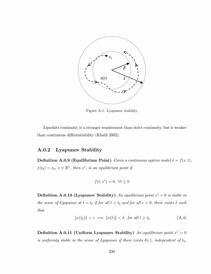
δ
ε
0x
)(tx
Figure A-1: Lyapunov stability
Lipschitz continuity is a stronger requirement than strict continuity, but is weaker
than continuous di¤erentiability (Khalil 2002).
A.0.2 Lyapunov Stability
De�nition A.0.9 (Equilibrium Point) Given a continuous system model _x = f(x; t),
x(t0) = x0, x 2 Rn, then x�, is an equilibrium point if
f(t; x�) = 0; 8t � 0
De�nition A.0.10 (Lyapunov Stability) An equilibrium point x� = 0 is stable in
the sense of Lyapunov at t = t0 if for all t > t0 and for all " > 0, there exists � such
that
kx(t0)k < " =) kx(t)k < �; for all t � t0 (A.4)
De�nition A.0.11 (Uniform Lyapunov Stability) An equilibrium point x� = 0
is uniformly stable in the sense of Lyapunov if there exists �("), independent of t0,
238
such that Eq. A.4 holds true.
Without loss of generality, the equilibrium point has been located at the origin for
the preceding de�nitions. In fact, it is possible for an equilibrium point to be located
anywhere in the state space of a system. Results for non-zero equilibrium points are
identical since an equilibrium can be translated from anywhere in the state space to
the origin.
De�nition A.0.12 (Unstable Equilibrium) An equilibrium point x� is unstable
if it is not stable.
239
AppendixBState Partitioning
In the case where additional partitions may need to be established on an already ex-
isting partitioned state space, the results of Lemma 3.2.4, Lemma 3.2.3 and Theorem
3.2.1 of Chapter 3 are extended here. The assumption is that we are starting with a
family of subsets H such that jHj =M and H is the result of a partitioning operation
that has already been applied to the state space such thatMSj=1
Qj = Rn.
Lemma B.0.1 (Set Partition Upper Bound) Let H = fQj � Rn : 1 � j � Mg
be a family of pairwise disjoint sets such thatMSj=1
Qj = Rn, and let = fFi : Rn !
R; 1 � i � Ng be a family of functionals. The set partition operation (II) of Def.
3.2.7,will produce a family of sets, H 0, such that jH 0j =M � 2N .
Proof. Show the upper bound by induction on the number of functionals, i, for
any jHj =M and assuming maximal intersection, which means that Qj \N (Fi) 6= ;
240
for all Qj 2 H and for all Fi 2 . The base case is for jj = 1 or N = 1 functionals:
jH 01j = P 1f (H;N (F )) =
����� MSj=1Ps(Qj;N (F ))�����
= jPs(Q1;N (F ))j+ jPs(Q2;N (F ))j+ : : :
+ jPs(QM ;N (F ))j
= 2 + 2 + : : :+ 2| {z }M
= 2M
= M � 2N
so the base case is consistent with the original hypothesis. The inductive hypothesis
is that jH 0N j =M�2N . It remains to show that
��H 0N+1
�� =M�2N+1. Due to maximal
intersection, Qj \N (FN+1) 6= ;, for all Qj 2 H 0N .
H 0N+1 = PN+1f (H 0
N ;N (FN+1)) =M�2NSj=1
Ps(Qj;N (FN+1))
and therefore,
��H 0N+1
�� =
������jH0
N jSj=1
Ps(Qj;N (FN+1))
������= jPs(Q1;N (FN+1))j+ jPs(Q2;N (F2))j+ : : :
+���Ps(QjH0
N j;N (FN+1))���
= 2 + 2 + : : :+ 2| {z }jH0
N j= 2� jH 0
N j and by the inductive hypothesis,
= 2�M � 2N
= M � 2N+1
241
Lemma B.0.2 (Set Partition Lower Bound) Let H = fQj � Rn : 1 � j � Mg
be a family of pairwise disjoint sets such thatMSj=1
Qj = Rn and let = fFi : Rn !
R; 1 � i � Ng be a family of functionals such that there is minimal intersection.
The set partition operation (II) of Def. 3.2.7,will produce a family of sets, H 0, such
that jH 0j =M +N .
Proof. The lower bound is proven by induction on the number of functionals,
i, for any jHj = M . The base case is for jj = 1 (i.e. N = 1). With minimal
intersection for example QM 2 H such that QM \N (F ) 6= ;, then
H 01 = P 1f (H;N (F1))
jH 01j =
�����M[j=2
Ps(Qj;N (F1))�����+ jPs(QM ;N (F1)j
= jPs(Q1;N (F1)j+ jPs(Q2;N (F1)j+ : : :
+ jPs(QM�1;N (F1)j
+ jPs(QM ;N (F1)j
= 1 + 1 + : : :+ 1| {z }M�1
+ 2
= M � 1 + 2
= M + 1
Thus the base case is consistent with the hypothesis. Now the inductive hypothesis
is that jH 0N j = M + N . It remains to show
��H 0N+1
�� = M + N + 1. Suppose there
exists QM+N 2 H 0N and jH 0
N j = jHN+1j then:
H 0N+1 = PN+1f (H 0
N ;N (FN+1)) =M+NSj=1
Ps(Qj;N (FN+1))
242
therefore
��H 0N+1
�� =
������jH0
N j�1Sj=1
Ps(Qj;N (FN+1))
������+���Ps(QjH0
N j;N (FN+1))���
= jPs(Q1;N (FN+1))j+ jPs(Q2;N (FN+1))j+ : : :
+���Ps(QjH0
N j�1;N (FN+1))���
+���Ps(QjH0
N j;N (FN+1))���
= 1 + 1 + : : :+ 1| {z }jH0
N j�1+ 2
= jH 0N j � 1 + 2; and by the inductive hypothesis,
= M +N + 1
Theorem B.0.1 (Set Partitioning Operation Boundedness) Let H = fQj �
Rn : 1 � j � Mg be a family of pairwise disjoint sets such thatMSj=1
Qj = Rn and let
= fFi : Rn ! R; 1 � i � Ng be a family of functionals. The set partition operation
(II) of Def. 3.2.7 produces a family of sets H 0, such that M +N � jH 0j �M � 2N .
Proof. Let jj = N , and let jHj = M it follows from Lemma B.0.2 that the
cardinality of the set partitioning operation has a lower bound of jH 0j = M + N .
Lemma B.0.1 establishes an upper bound on the returned family of sets of jH 0j =
M � 2N , hence the result is proven.
243
AppendixCDiscrete Event System Modeling
C.1 Finite State Machines
The �nites state machine (FSM) model is one of many possible representations of a
discrete event system (DES), and has been used extensively since it lends itself readily
to the analysis of such systems.
De�nition C.1.1 A deterministic FSM model is a �ve-tuple:
G = (X;�;�; x0; Xm)
where:
X is the set of states,
� is the set of events that cause G to change states
� is the transition set, the set of all labeled transitions
x0 is the initial state, x0 2 X
Xm is the set of marked states, Xm � X
244
De�nition C.1.2 A transition function is de�ned in G denoted by �(x; �)! with x 2
X, � 2 ��, if 9x 2 X and (x; �; �x) 2 �.
De�nition C.1.3 The language generated by G, L(G), is the set of all symbols and
concatenated symbols (strings) that would be generated by starting at x0 and exercising
all possible transitions in sequence across the entire state space of the automaton.
De�nition C.1.4 The language marked by G, Lm(G), is the set of all strings s, for
which �(x0; s)! in G and �(x0; s) 2 Xm. The marked states represent the completion
of some task and the strings s, are able to take the system from the initial condition
to the completion of the task, a marked state.
De�nition C.1.5 Two automata, G1 and G2, are said to be equivalent if L(G1) =
L(G2) and Lm(G1) = Lm(G2).
De�nition C.1.6 The language L(G2) is said to be a sublanguage of L(G1) if 8s 2
L(G2); s 2 L(G1)) L(G1) � L(G2).
The event set of the generator G, is partitioned, � = �uc [ �c where �uc is the
set of uncontrollable events and �c is the set of controllable events.
The graphical representation of a hypothetical machine modeled by a FSM is
pictured in Fig. C-1. In the �gure, states are labeled and are represented by the
nodes of the graph. The arcs connecting the nodes are state transitions and are
labeled with events. A single-ended arc pointing into a node denotes the initial state.
Marked states are denoted by a double circle.The initial state of the system, x0 is the
Idle state (labeled I), indicated by the arrow pointing in; it is also a marked state.
Other states in the system are Working (W, marked), Down (D), and Scrapped (S),
X = fI;W;D; Sg. The marker states are Xm = fI;Wg. The machine�s event set is
� = f�; �; �; �; �; �g, with the event labels representing the following actions:
� the machine starts, Idle to Working,
245
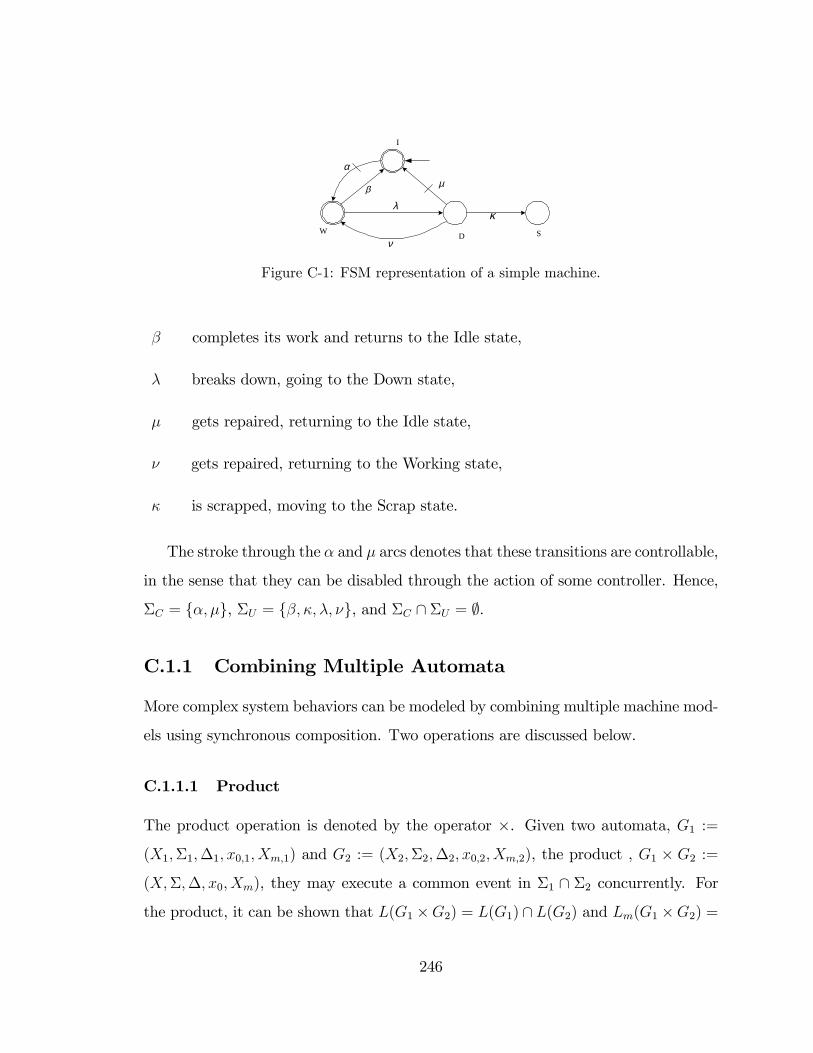
µ
α
β
ν
λκ
I
W D S
Figure C-1: FSM representation of a simple machine.
� completes its work and returns to the Idle state,
� breaks down, going to the Down state,
� gets repaired, returning to the Idle state,
� gets repaired, returning to the Working state,
� is scrapped, moving to the Scrap state.
The stroke through the � and � arcs denotes that these transitions are controllable,
in the sense that they can be disabled through the action of some controller. Hence,
�C = f�; �g, �U = f�; �; �; �g, and �C \ �U = ;.
C.1.1 Combining Multiple Automata
More complex system behaviors can be modeled by combining multiple machine mod-
els using synchronous composition. Two operations are discussed below.
C.1.1.1 Product
The product operation is denoted by the operator �. Given two automata, G1 :=
(X1;�1;�1; x0;1; Xm;1) and G2 := (X2;�2;�2; x0;2; Xm;2), the product , G1 � G2 :=
(X;�;�; x0; Xm), they may execute a common event in �1 \ �2 concurrently. For
the product, it can be shown that L(G1 �G2) = L(G1) \ L(G2) and Lm(G1 �G2) =
246
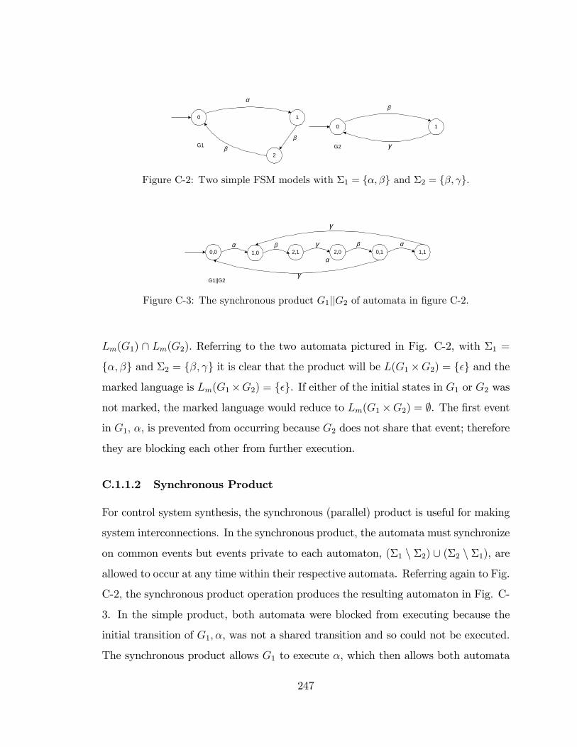
2
10
βγ
β
10
βG1 G2
α
Figure C-2: Two simple FSM models with �1 = f�; �g and �2 = f�; g:
α0,0 1,0 2,1 2,0 0,1 1,1
γ
β βγ
γ
α
α
G1||G2
Figure C-3: The synchronous product G1jjG2 of automata in �gure C-2.
Lm(G1) \ Lm(G2). Referring to the two automata pictured in Fig. C-2, with �1 =
f�; �g and �2 = f�; g it is clear that the product will be L(G1�G2) = f�g and the
marked language is Lm(G1�G2) = f�g. If either of the initial states in G1 or G2 was
not marked, the marked language would reduce to Lm(G1�G2) = ;. The �rst event
in G1; �, is prevented from occurring because G2 does not share that event; therefore
they are blocking each other from further execution.
C.1.1.2 Synchronous Product
For control system synthesis, the synchronous (parallel) product is useful for making
system interconnections. In the synchronous product, the automata must synchronize
on common events but events private to each automaton, (�1 n �2) [ (�2 n �1), are
allowed to occur at any time within their respective automata. Referring again to Fig.
C-2, the synchronous product operation produces the resulting automaton in Fig. C-
3. In the simple product, both automata were blocked from executing because the
initial transition of G1; �, was not a shared transition and so could not be executed.
The synchronous product allows G1 to execute �, which then allows both automata
247
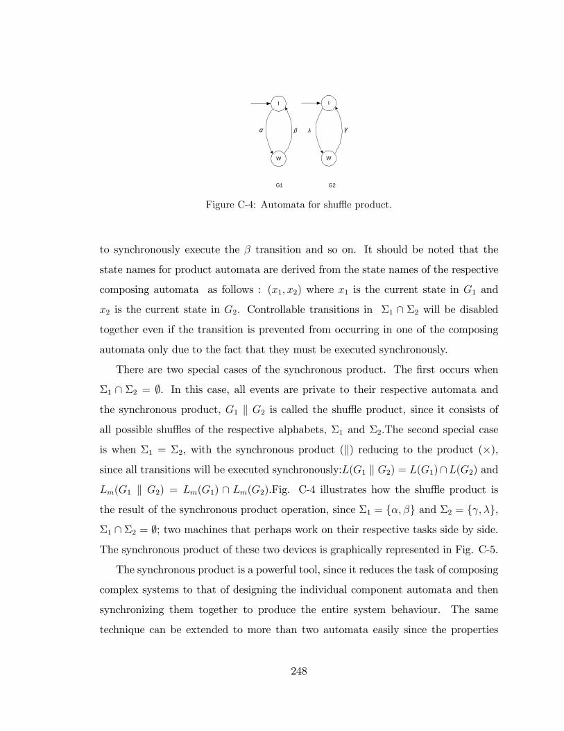
I
W
γβ
G1
α
I
W
λ
G2
Figure C-4: Automata for shu e product.
to synchronously execute the � transition and so on. It should be noted that the
state names for product automata are derived from the state names of the respective
composing automata as follows : (x1; x2) where x1 is the current state in G1 and
x2 is the current state in G2. Controllable transitions in �1 \ �2 will be disabled
together even if the transition is prevented from occurring in one of the composing
automata only due to the fact that they must be executed synchronously.
There are two special cases of the synchronous product. The �rst occurs when
�1 \ �2 = ;. In this case, all events are private to their respective automata and
the synchronous product, G1 k G2 is called the shu e product, since it consists of
all possible shu es of the respective alphabets, �1 and �2.The second special case
is when �1 = �2, with the synchronous product (k) reducing to the product (�),
since all transitions will be executed synchronously:L(G1 k G2) = L(G1)\L(G2) and
Lm(G1 k G2) = Lm(G1) \ Lm(G2).Fig. C-4 illustrates how the shu e product is
the result of the synchronous product operation, since �1 = f�; �g and �2 = f ; �g,
�1 \ �2 = ;; two machines that perhaps work on their respective tasks side by side.
The synchronous product of these two devices is graphically represented in Fig. C-5.
The synchronous product is a powerful tool, since it reduces the task of composing
complex systems to that of designing the individual component automata and then
synchronizing them together to produce the entire system behaviour. The same
technique can be extended to more than two automata easily since the properties
248
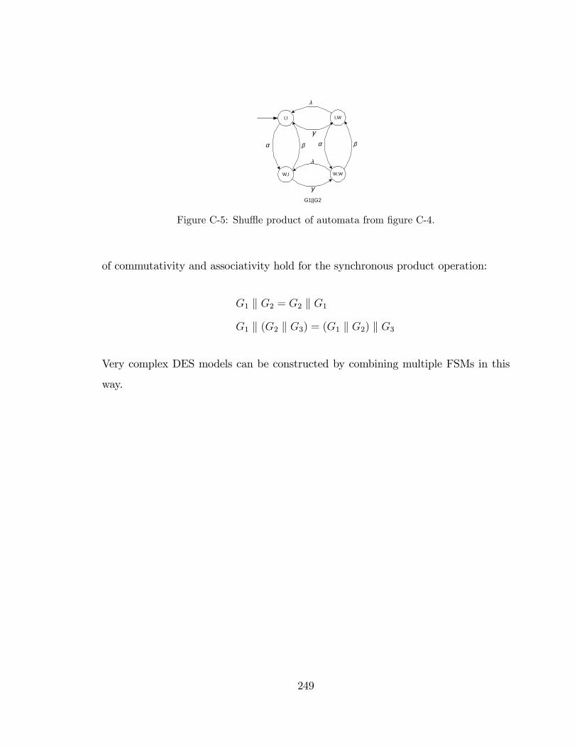
I,I
W,I
γ
βα
I,W
W,W
λ
α β
γ
λ
G1||G2
Figure C-5: Shu e product of automata from �gure C-4.
of commutativity and associativity hold for the synchronous product operation:
G1 k G2 = G2 k G1
G1 k (G2 k G3) = (G1 k G2) k G3
Very complex DES models can be constructed by combining multiple FSMs in this
way.
249
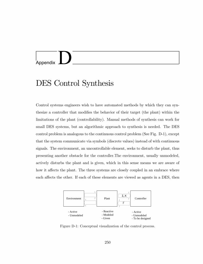
AppendixDDES Control Synthesis
Control systems engineers wish to have automated methods by which they can syn-
thesize a controller that modi�es the behavior of their target (the plant) within the
limitations of the plant (controllability). Manual methods of synthesis can work for
small DES systems, but an algorithmic approach to synthesis is needed. The DES
control problem is analogous to the continuous control problem (See Fig. D-1), except
that the system communicate via symbols (discrete values) instead of with continuous
signals. The environment, an uncontrollable element, seeks to disturb the plant, thus
presenting another obstacle for the controller.The environment, usually unmodeled,
actively disturbs the plant and is given, which in this sense means we are aware of
how it a¤ects the plant. The three systems are closely coupled in an embrace where
each a¤ects the other. If each of these elements are viewed as agents in a DES, then
Environment Plant Controller
Active Unmodeled
Reactive Modeled Given
Active
To be designed
Γ
ΧΣ,
Unmodeled
Figure D-1: Conceptual visualization of the control process.
250
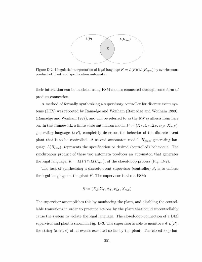
)(PL )( SpecHL
K
Figure D-2: Linguistic interpretation of legal language K = L(P )\L(Hspec) by synchronousproduct of plant and speci�cation automata.
their interaction can be modeled using FSM models connected through some form of
product connection.
A method of formally synthesizing a supervisory controller for discrete event sys-
tems (DES) was reported by Ramadge and Wonham (Ramadge and Wonham 1989),
(Ramadge and Wonham 1987), and will be referred to as the RW synthesis from here
on. In this framework, a �nite state automaton model P := (XP ;�P ;�P ; x0;P ; Xm;P ),
generating language L(P ), completely describes the behavior of the discrete event
plant that is to be controlled. A second automaton model, Hspec, generating lan-
guage L(Hspec), represents the speci�cation or desired (controlled) behaviour. The
synchronous product of these two automata produces an automaton that generates
the legal language, K = L(P ) \ L(Hspec), of the closed-loop process (Fig. D-2).
The task of synthesizing a discrete event supervisor (controller) S, is to enforce
the legal language on the plant P . The supervisor is also a FSM:
S := (XS;�S;�S; x0;S; Xm;S)
The supervisor accomplishes this by monitoring the plant, and disabling the control-
lable transitions in order to preempt actions by the plant that could uncontrollably
cause the system to violate the legal language. The closed-loop connection of a DES
supervisor and plant is shown in Fig. D-3. The supervisor is able to monitor s 2 L(P ),
the string (a trace) of all events executed so far by the plant. The closed-loop lan-
251
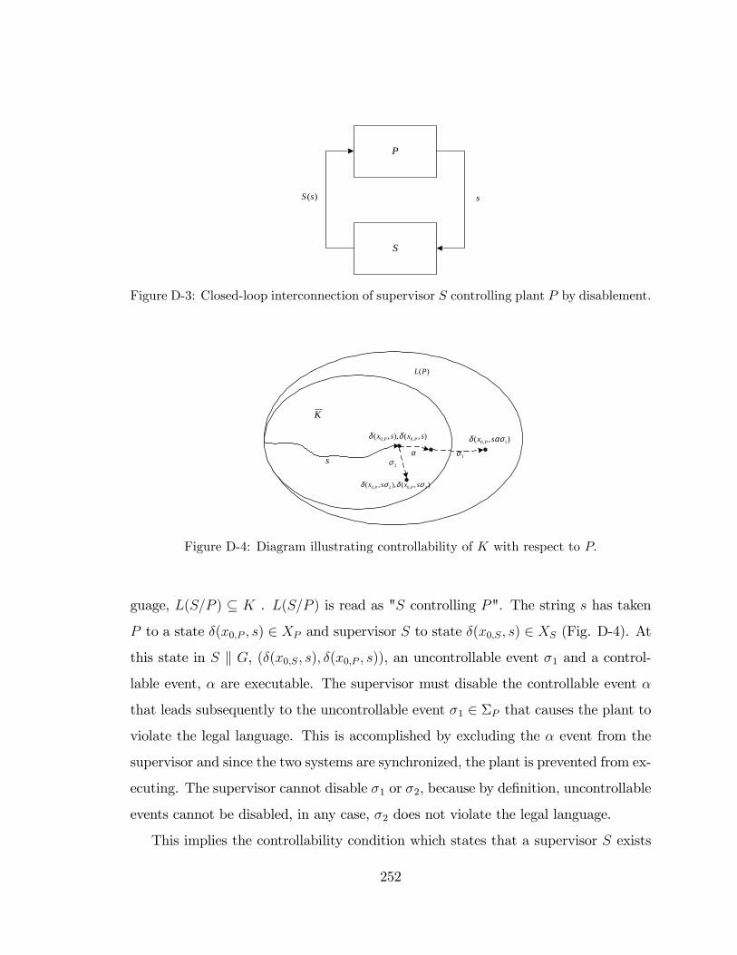
P
S
)(sS s
Figure D-3: Closed-loop interconnection of supervisor S controlling plant P by disablement.
K
),(),,( ,0,0 sxsx PP δδ
s
)(PL
),( 1,0 ασδ sx P
1σ2σ
),(),,( 2,02,0 σδσδ sxsx PP
α
Figure D-4: Diagram illustrating controllability of K with respect to P:
guage, L(S=P ) � K . L(S=P ) is read as "S controlling P". The string s has taken
P to a state �(x0;P ; s) 2 XP and supervisor S to state �(x0;S; s) 2 XS (Fig. D-4). At
this state in S k G, (�(x0;S; s); �(x0;P ; s)), an uncontrollable event �1 and a control-
lable event, � are executable. The supervisor must disable the controllable event �
that leads subsequently to the uncontrollable event �1 2 �P that causes the plant to
violate the legal language. This is accomplished by excluding the � event from the
supervisor and since the two systems are synchronized, the plant is prevented from ex-
ecuting. The supervisor cannot disable �1 or �2, because by de�nition, uncontrollable
events cannot be disabled, in any case, �2 does not violate the legal language.
This implies the controllability condition which states that a supervisor S exists
252
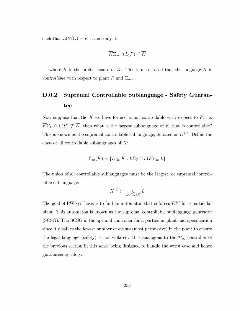
such that L(S=G) = K if and only if:
K�uc \ L(P ) � K
where K is the pre�x closure of K. This is also stated that the language K is
controllable with respect to plant P and �uc.
D.0.2 Supremal Controllable Sublanguage - Safety Guaran-
tee
Now suppose that the K we have formed is not controllable with respect to P , i.e.
K�U \ L(P ) * K, then what is the largest sublanguage of K that is controllable?
This is known as the supremal controllable sublanguage, denoted as K"C . De�ne the
class of all controllable sublanguages of K:
Cin(K) = fL � K : L�U \ L(P ) � Lg
The union of all controllable sublanguages must be the largest, or supremal control-
lable sublanguage:
K"C := [L2Cin(K)
L
The goal of RW synthesis is to �nd an automaton that enforces K"C for a particular
plant. This automaton is known as the supremal controllable sublanguage generator
(SCSG). The SCSG is the optimal controller for a particular plant and speci�cation
since it disables the fewest number of events (most permissive) in the plant to ensure
the legal language (safety) is not violated. It is analogous to the H1 controller of
the previous section in this sense being designed to handle the worst case and hence
guaranteeing safety.
253
D.0.3 In�mal Controllable Sublanguage - Performance Guar-
antee
De�ning the class of pre�x-closed, controllable superlanguages:
Cout(K) = fL � �� : (K � L � L(P )) ^ (L = L) ^ (L�uc \ L(P ) � L)g
The in�mal controllable superlanguage is the intersection of all controllable superlan-
guages:
K#C := \L2Cout(K)
L
If K represents the minimal required language of a plant as opposed to the maximum
legal behaviour, then the automaton that enforces K#C is the smallest (optimal) con-
troller that can be guarantees that the closed-loop system will meet this speci�cation.
Optimal with respect to performance.
To summarize the relationship between each of the languages:
; � K"C � K � K � K#C � L(P )
where
K"C is the supremal controllable sublanguage,
K is the maximum legal language, or minimum performance,
K is the pre�x closure of K,
K#C is the in�mal pre�x-closed controllable superlanguage,
L(P ) is the plant language.
254
D.0.4 Nonblocking Controllability
A desirable feature of a supervisory controller is nonblocking behaviour, also known
as liveness. So in addition to the controllability condition on the legal language,
K�uc \ L(P ) � K, the legal language must also be non-blocking:
K = K \ Lm(P )
That is, the controller should not able to "stop" execution at an unmarked state in
P . So the following is true of a nonblocking supervisor:
Lm(S=P ) = (Lm(P ) \ Lm(Hspec))"C
L(S=P ) = (Lm(P ) \ Lm(Hspec))"C
D.1 DES Controller Synthesis Software
Several software packages are available that implement the RW synthesis, including
TCT, OTCT and UMDES (University of Michigan DES library). The �rst package
was TCT, developed at the University of Toronto. A similar and related software
package is OTCT, which has a script-based interface as opposed to a menu-based
GUI. OTCT lends itself better to automated operation, since jobs are submitted in
as a batch using the scripting language. Automata are speci�ed using a text �le
description. Once read into the OTCT workspace, the automata are represented
as objects and can be manipulated with various functions. The three that shall be
considered here are:
� sync(x,y): forms the synchronous product of two argument objects, x and y,
� supfcBySync(x,y): computes the maximally permissive controller given the
plant,x, and the generator of the speci�cation, y,
255
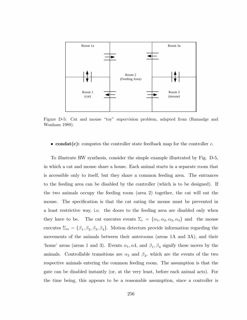
Room 2(Feeding Area)
Room 1a
Room 1(cat)
Room 3a
Room 3(mouse)
Figure D-5: Cat and mouse �toy� supervision problem, adapted from (Ramadge andWonham 1989).
� condat(c): computes the controller state feedback map for the controller c.
To illustrate RW synthesis, consider the simple example illustrated by Fig. D-5,
in which a cat and mouse share a house. Each animal starts in a separate room that
is accessible only to itself, but they share a common feeding area. The entrances
to the feeding area can be disabled by the controller (which is to be designed). If
the two animals occupy the feeding room (area 2) together, the cat will eat the
mouse. The speci�cation is that the cat eating the mouse must be prevented in
a least restrictive way, i.e. the doors to the feeding area are disabled only when
they have to be. The cat executes events �c = f�1; �2; �3; �4g and the mouse
executes �m = f�1; �2; �3; �4g. Motion detectors provide information regarding the
movements of the animals between their anterooms (areas 1A and 3A), and their
�home�areas (areas 1 and 3). Events �1; �4; and �1; �4 signify these moves by the
animals. Controllable transitions are �2 and �2, which are the events of the two
respective animals entering the common feeding room. The assumption is that the
gate can be disabled instantly (or, at the very least, before each animal acts). For
the time being, this appears to be a reasonable assumption, since a controller is
256
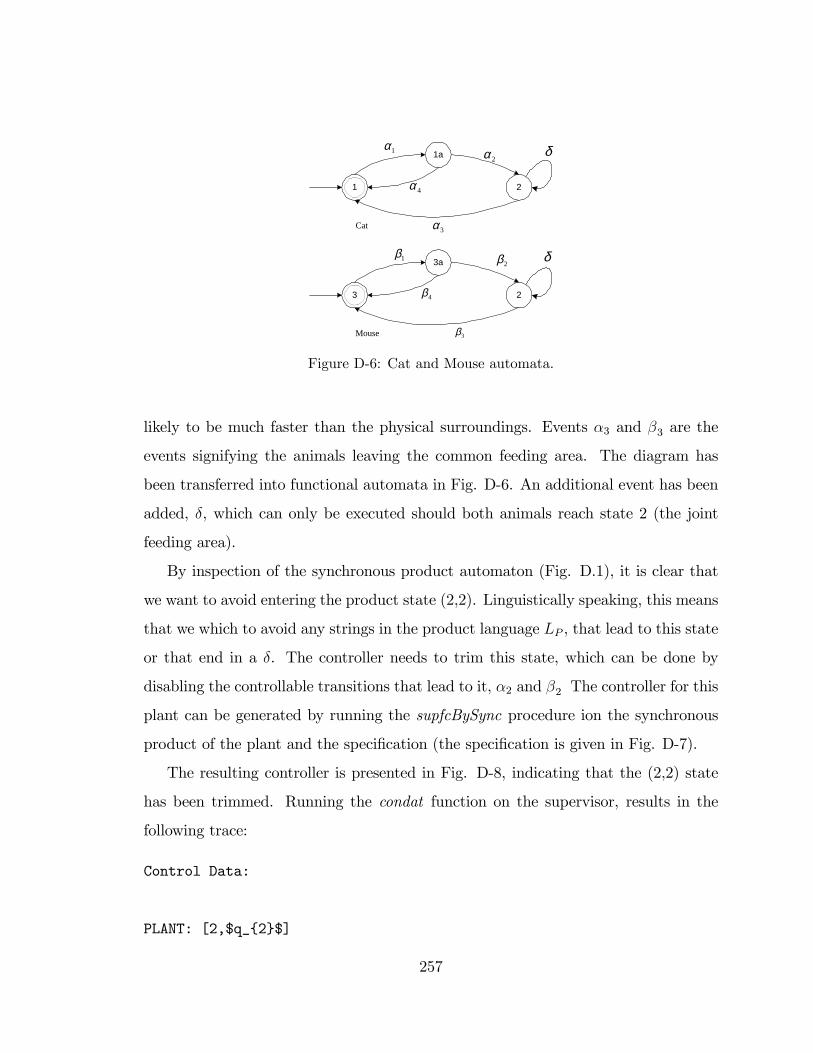
21
1α1a 2α
3α
4α
23
1β3a 2β
3β
4β
δ
δ
Cat
Mouse
Figure D-6: Cat and Mouse automata.
likely to be much faster than the physical surroundings. Events �3 and �3 are the
events signifying the animals leaving the common feeding area. The diagram has
been transferred into functional automata in Fig. D-6. An additional event has been
added, �, which can only be executed should both animals reach state 2 (the joint
feeding area).
By inspection of the synchronous product automaton (Fig. D.1), it is clear that
we want to avoid entering the product state (2,2). Linguistically speaking, this means
that we which to avoid any strings in the product language LP , that lead to this state
or that end in a �. The controller needs to trim this state, which can be done by
disabling the controllable transitions that lead to it, �2 and �2 The controller for this
plant can be generated by running the supfcBySync procedure ion the synchronous
product of the plant and the speci�cation (the speci�cation is given in Fig. D-7).
The resulting controller is presented in Fig. D-8, indicating that the (2,2) state
has been trimmed. Running the condat function on the supervisor, results in the
following trace:
Control Data:
PLANT: [2,$q_{2}$]
257
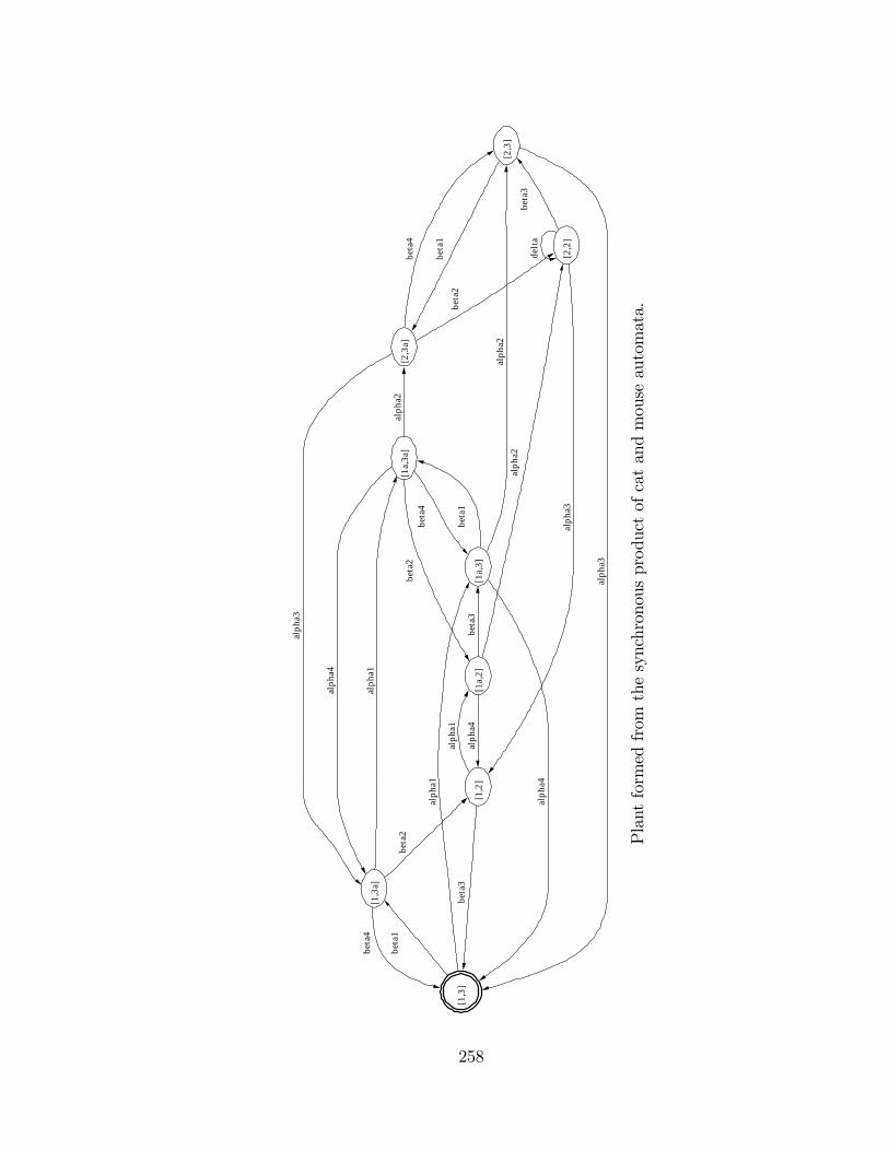
[1,3
]
[1,3
a]
beta
1
[1a,
3]
alph
a1
beta
4
[1a,
3a]
alph
a1
[1,2
]
beta
2
alph
a4
[2,3
]al
pha2
beta
1
alph
a3
[2,3
a]
beta
1
alph
a4
beta
4
alph
a2
[1a,
2]
beta
2
alph
a3
beta
4
[2,2
]
beta
2
beta
3al
pha4
alph
a2
beta
3al
pha1
beta
3
alph
a3
delt
a
Plantformedfrom
thesynchronousproductofcatandmouseautomata.
258
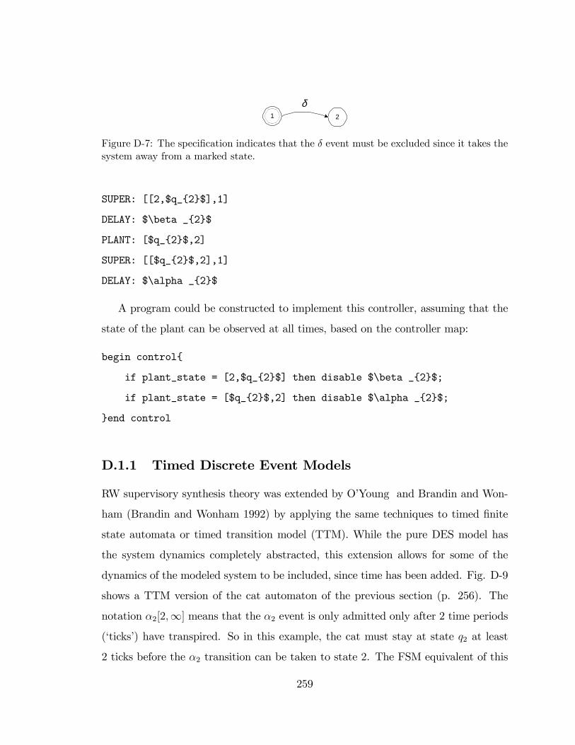
2
δ1
Figure D-7: The speci�cation indicates that the � event must be excluded since it takes thesystem away from a marked state.
SUPER: [[2,$q_{2}$],1]
DELAY: $\beta _{2}$
PLANT: [$q_{2}$,2]
SUPER: [[$q_{2}$,2],1]
DELAY: $\alpha _{2}$
A program could be constructed to implement this controller, assuming that the
state of the plant can be observed at all times, based on the controller map:
begin control{
if plant_state = [2,$q_{2}$] then disable $\beta _{2}$;
if plant_state = [$q_{2}$,2] then disable $\alpha _{2}$;
}end control
D.1.1 Timed Discrete Event Models
RW supervisory synthesis theory was extended by O�Young and Brandin and Won-
ham (Brandin and Wonham 1992) by applying the same techniques to timed �nite
state automata or timed transition model (TTM). While the pure DES model has
the system dynamics completely abstracted, this extension allows for some of the
dynamics of the modeled system to be included, since time has been added. Fig. D-9
shows a TTM version of the cat automaton of the previous section (p. 256). The
notation �2[2;1] means that the �2 event is only admitted only after 2 time periods
(�ticks�) have transpired. So in this example, the cat must stay at state q2 at least
2 ticks before the �2 transition can be taken to state 2. The FSM equivalent of this
259
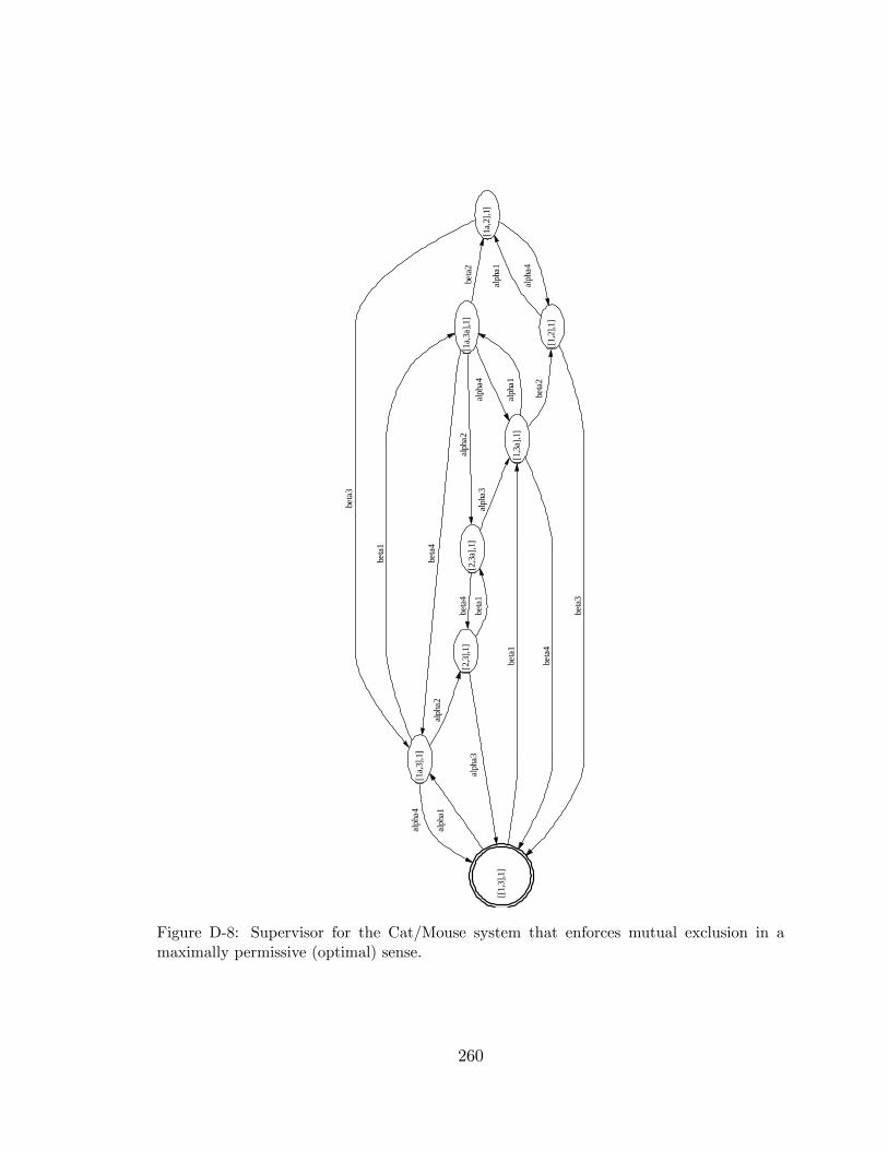
[[1,
3],1
]
[[1a
,3],1
]
alph
a1
[[1,
3a],1
]be
ta1
alph
a4
[[1a
,3a]
,1]
beta
1
[[2,
3],1
]
alph
a2
beta
4
alph
a1
[[1,
2],1
]be
ta2
beta
4
alph
a4[[
2,3a
],1]
alph
a2
[[1a
,2],1
]
beta
2al
pha3
beta
1al
pha3
beta
4
beta
3
alph
a4
beta
3
alph
a1
Figure D-8: Supervisor for the Cat/Mouse system that enforces mutual exclusion in amaximally permissive (optimal) sense.
260
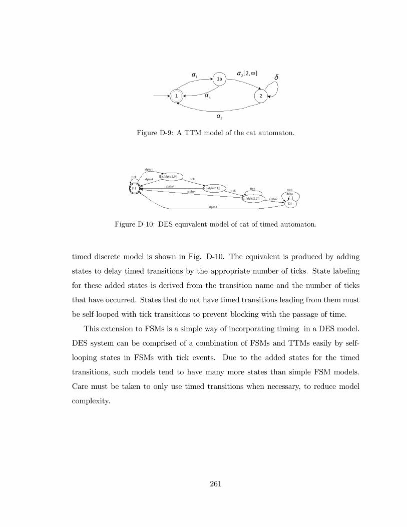
21
1α1a
],2[2 ∞α
3α
4α
δ
Figure D-9: A TTM model of the cat automaton.
[1]
tick [1a,[alpha2,0]]
alpha1
alpha4
[1a,[alpha2,1]]
tick
alpha4
[1a,[alpha2,2]]
tickalpha4tick
[2]alpha2
alpha3
tickdelta
Figure D-10: DES equivalent model of cat of timed automaton.
timed discrete model is shown in Fig. D-10. The equivalent is produced by adding
states to delay timed transitions by the appropriate number of ticks. State labeling
for these added states is derived from the transition name and the number of ticks
that have occurred. States that do not have timed transitions leading from them must
be self-looped with tick transitions to prevent blocking with the passage of time.
This extension to FSMs is a simple way of incorporating timing in a DES model.
DES system can be comprised of a combination of FSMs and TTMs easily by self-
looping states in FSMs with tick events. Due to the added states for the timed
transitions, such models tend to have many more states than simple FSM models.
Care must be taken to only use timed transitions when necessary, to reduce model
complexity.
261
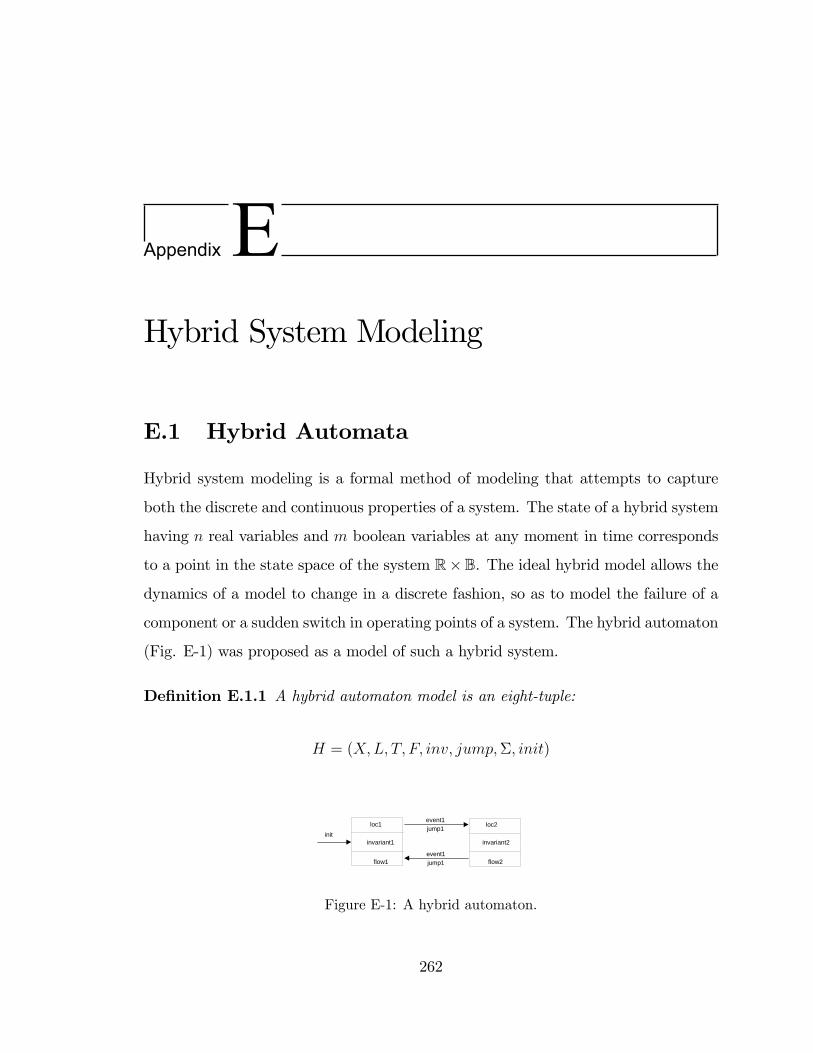
AppendixEHybrid System Modeling
E.1 Hybrid Automata
Hybrid system modeling is a formal method of modeling that attempts to capture
both the discrete and continuous properties of a system. The state of a hybrid system
having n real variables and m boolean variables at any moment in time corresponds
to a point in the state space of the system R�B. The ideal hybrid model allows the
dynamics of a model to change in a discrete fashion, so as to model the failure of a
component or a sudden switch in operating points of a system. The hybrid automaton
(Fig. E-1) was proposed as a model of such a hybrid system.
De�nition E.1.1 A hybrid automaton model is an eight-tuple:
H = (X;L; T; F; inv; jump;�; init)
loc2init
loc1
flow1
invariant1 invariant2
flow2
event1jump1
event1jump1
Figure E-1: A hybrid automaton.
262
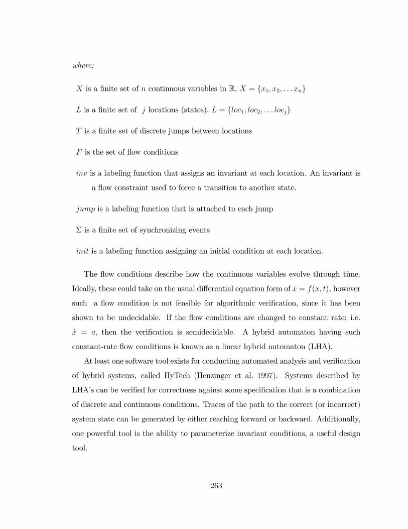
where:
X is a �nite set of n continuous variables in R, X = fx1; x2; : : : xng
L is a �nite set of j locations (states), L = floc1; loc2; : : : locjg
T is a �nite set of discrete jumps between locations
F is the set of �ow conditions
inv is a labeling function that assigns an invariant at each location. An invariant is
a �ow constraint used to force a transition to another state.
jump is a labeling function that is attached to each jump
� is a �nite set of synchronizing events
init is a labeling function assigning an initial condition at each location.
The �ow conditions describe how the continuous variables evolve through time.
Ideally, these could take on the usual di¤erential equation form of _x = f(x; t), however
such a �ow condition is not feasible for algorithmic veri�cation, since it has been
shown to be undecidable. If the �ow conditions are changed to constant rate; i.e.
_x = a; then the veri�cation is semidecidable. A hybrid automaton having such
constant-rate �ow conditions is known as a linear hybrid automaton (LHA).
At least one software tool exists for conducting automated analysis and veri�cation
of hybrid systems, called HyTech (Henzinger et al. 1997). Systems described by
LHA�s can be veri�ed for correctness against some speci�cation that is a combination
of discrete and continuous conditions. Traces of the path to the correct (or incorrect)
system state can be generated by either reaching forward or backward. Additionally,
one powerful tool is the ability to parameterize invariant conditions, a useful design
tool.
263
AppendixFHySynth: Hybrid Control Synthesis
Software Package
F.1 Introduction
The HySynth software package was developed to implement the concepts that have
been set forth in this thesis. HySynth is an object-oriented package that allows for
hybrid system modeling and controller synthesis, hence the name Hy (for Hybrid)
and Synth (for Controller Synthesis). The package allows for the modeling and syn-
thesis of controllers using a combination of SC models and FS models. HySynth
was developed within the Mathworks�Matlab environment, thus allowing it to take
advantage of the numerous ODE solvers and the many other toolboxes that are avail-
able to Matlab users. This permits a designer the �exibility to embed existing Matlab
simulations within the switched continuous model framework.
F.2 Brief Overview
The HySynth package has been developed using the object-oriented features of Mat-
lab. A number of objects are available for constructing hybrid models, and various
264
commands are available to manipulate models and to synthesize and simulate con-
trollers. The methods associated with each object extend the basic functionality of
Matlab script. Application examples of HySynth are detailed in Chapter 7.
F.2.1 Objects
The modeling objects are:
fsm This is the basic DES building block, the �nite state automaton model. An
fsm object can be constructed graphically by the JFLAP GUI and stored to an
XML �le. The constructor method is then invoked to instantiate the object;
e.g. m1=fsm(�m1.xml�);. Once created, the object is referred to by its variable
name, m1. Alternatively, the �nite state machine object can be created pro-
grammatically by de�ning the various sets: the state set, event set, transition
function, and so on.
scm The basic switched continuous system model. Currently no GUI has been de-
signed for the scm object, so it must be constructed using a Matlab script. The
user de�nes a set of continuous dynamics, as Matlab function handles, which
point to the desired continuous system models. The continuous systems are cap-
tured as Matlab functions in the form of a generalized nonlinear time-varying
di¤erential equation; i.e. _x = f(x; t; params). A corresponding set of input
event labels should be de�ned, one label for each continuous system model.
Partitioning functionals are de�ned via an event function that implements the
event detection in conjunction with the Matlab ODE solvers. For each partition,
a set of output event labels must be de�ned.
product The synchronous product object, a hierarchical object made up of fsm, scm
or other product objects. For example, given a pair of existing FSM objects,
m1 and m2, the product constructor function is used as follows to create their
product: p1 = product(m1,m2).
265
The state objects are:
finiteState The �nite state object, a �nite state label, a Matlab string.
ctsState The continuous state object, storage of continuous (state) variables x 2 Rn,
a Matlab double vector.
pstate The product state object. A hierarchical object, made up of two or more
finiteState, ctsState, or other pstate objects.
F.2.2 Commands
Once a system model has been constructed, various methods are available to modify
it, analyze it, and to view its structure. This section contains a partial listing of
commands that a user needs to create a controller structure.
Commands that apply to fsm objects only:
addEvents adds the argument list of events to the event set
markAll mark all of the states as ESD states.
unMarkAll unmark all ESD states.
addEvents adds the argument list of events to the event set
Commands common to all modeling objects:
initial returns the initial state of a system model
printAsDot print the argument object as a Graphviz format �le in .dot format to
the argument �lename.
printAsPs print the argument object as an Adobe PostScript format �le to the ar-
gument �lename.
266
printAsPDF print the argument object as an Adobe PDF format �le to the argument
�lename.
printAs*WithEvents print limited event lookahead (reachability) of the argument
object to the argument �lename. Prints to one of three �le formats, replace
wildcard * with one of Dot, Ps or PDF.
printAs*WithTime print limited time lookahead (reachability) of the argument ob-
ject to the argument �lename. Prints to one of three �le formats, replace wild-
card * with one of Dot, Ps or PDF.
simulate given an argument input event, performs a prediction until the next choice
point.
267