Online Data Appendix for“Multilateral Trade Bargaining:

A First Look at theGATT Bargaining Records”

Kyle Bagwell Robert W. Staiger Ali Yurukoglu

July 2017

1. Data Appendix

In this appendix, we detail the steps we have taken to process the Torquay bargaining recordsinto a format for analysis. The most challenging step in this process was creating a concordanceof product descriptions from the Torquay records to the HS6 1988 product codes. Below wedefine the data elements that we extracted from the bargaining records, and then we discussthe concordance process which we applied to the bargaining records.

1.1. Bargaining Records

The first major task in assembling the dataset was to transfer the information from the scannedbargaining records posted on the WTO web site to a workable spreadsheet. We accomplishedthis in two steps. In a first step we hired transcribers to enter into Excel exactly what appearedon the original scans. Then in a second step, we transferred the raw Excel data into a bargainingrecord template that we created as a way to standardize the structure of the data for each ofthe bilateral negotiations.

We used the following set of variables as the template for how each bargaining record wasinput into the complete spreadsheet. The list below gives the field title (in bold), an exampleentry (in italics), and a more detailed description of the meaning of the field. The exampleincluded below is taken from the negotiations between Australia and the United States.

1. Bargaining Partners: United States and Australia. Countries engaging in a givenbilateral bargain.

2. Proposal Date: 10/25/1950. Date on which the document was submitted.

3. Proposer Country: Australia. Country submitting the document.

Figure 1.1: An example item from the US-Australia bargaining records.

4. Proposal Type (Request, Offer, Modification of Request, Modification of Of-fer, Final Offer): Offer. Nature of the content of the document; in the example,Australia is making an offer to the US.

5. Target Country: United States. Country to whom the document is being submitted forreview/approval.

6. Currency: Australian Pound (“s.d”). Currency used in the document.

7. Tariff Item No.: 178(C)(1). If available, item number in the tariff schedule of thetariff-cutting country.

8. Statistical Class Number: (blank). If available, the item number for the good of whichthe concession is requested/offered, taken from the tariff-cutting country’s trade data (keyin determining negotiating rights through principal supplier).

9. Description of Products: Valves for internal combustion engines - The weight of whichdoes not exceed one pound each. Description of the product in the bargaining record.

10. Duty Unit (Specific Only): per lb. Units used for a specific tariff.

11. History of Tariffs: Act of 1930: (blank). Tariff resulting from the Smoot-HawleyTariff Act in 1930 (US only).

12. History of Tariffs: January 1, 1945: (blank). Tariff in effect as of the commencementof GATT (in the current dataset, only reported by the US on concession offers made).

13. Present Duty Rate: MFN Tariff : MFN tariff rate in effect at the beginning ofthe round of negotiations. Base date is November 15, 1949 for the Torquay round(GATT/CP/43, page 5).

(i) Specific: 2/9

(ii) Ad Valorem: 0.4750

(iii) Both (IF BOTH: Maximum/Minimum/Combination): Maximum.

2

14. Present Duty Rate: Additional Surtax: (blank).

15. Present Duty Rate: MFN Primage: 0.1000. Additional ad valorem import dutylevied by customs (used exclusively by Australia in current dataset).

16. Present Duty Rate: Preferential Tariff : MFN tariff rate in effect at the beginningof the round of negotiations.

(i) Specific: 1/6

(ii) Ad Valorem: 0.2250

(iii) Both (IF BOTH: Maximum/Minimum/Combination): Maximum.

17. Present Duty Rate: Preferential Primage: 0.0500. Additional ad valorem importduty levied by customs (used exclusively by Australia in current dataset).

18. Requested or Offered Duty Rate: MFN Tariff : The requested or offered modifiedMFN tariff rate. Because the example is of Australia’s offer, the remaining parts ofthis specific record item are all offers (the US request of “30%. Eliminate specific rate.Eliminate Primage.” would be listed in the corresponding earlier bargaining record item).

(i) Specific: 2/6

(ii) Ad Valorem: 0.3750

(iii) Both (IF BOTH: Maximum/Minimum/Combination): Maximum.

19. Requested or Offered Tariff Binding (Denoted by ‘b’): (blank). Binary variableindicating if the country specifically requested that the tariff be bound against futureincreases. In this case, the US did not specifically request that Australia bind the tariffagainst future increase.

20. Requested or Offered Duty Rate: Additional Surtax: (blank).

21. Requested or Offered Duty Rate: MFN Primage: Exempt.

22. Requested or Offered Duty Rate: Preferential Tariff : Requested adjustments toany preferential tariff rates.

(i) Specific: 1/6

(ii) Ad Valorem: 0.2250

(iii) Both (IF BOTH: Maximum/Minimum/Combination): Maximum.

23. Requested or Offered Duty Rate: Preferential Primage: Exempt.

24. Remarks: BPT. Any additional information included that is beyond the scope of theother entries. The note here is specifying that the above preferential rates are the BritishPreferential Tariff rates.

25. Negotiation Status (Continuing/Terminated/Successfully completed): Contin-uing. An indication of the stage of the bilateral negotiation.

3

1.2. Concording Bargaining Data to the Harmonized System

We used a multistage process to assign the relevant 1988 HS6 codes to each of the items inthe Torquay bargaining records. The first stage consisted of applying existing concordancesto the bargaining records. In the second stage, products that were not successfully matchedin stage one were matched using an automated string-matching score-function approach. Thisapproach assigned candidate concordances to a bargaining record product description based onthe similarity of the description to the HS6 product descriptions. For products still unsuccess-fully matched after the first two stages, the final stage was the manual assignment of HS6 codesbased on human judgment and research.

First stage. Instead of trying to match across the 40-year gap between the Torquayround descriptions and the HS 1988 product descriptions, whenever possible we matched acrosssmaller time gaps using product classifications from four points in time. This strategy enabledus to more accurately match products and it allowed us to use existing concordances to coverpart of the time gap. We began by assigning Schedule A 1948 product codes (taken from“Schedule A: Statistical Classification of Imports into the United States”) to the bargainingrecords.1 Next, we matched Schedule A 1948 product descriptions to a later version of ScheduleA (published in 1963). Matching to different versions of the same classification system wasrelatively straightforward even with the 15 year time gap. We then matched the 1963 ScheduleA codes to the TSUSA product codes from 1972. Once we had concorded to the 1972 TSUSAcodes, we used the concordance from TSUSA 1972 to HS6 1988 created by Robert Feenstra andhis colleagues at the Center for International Data as a part of their work creating the worldtrade database.

The US included its Schedule A 1948 product codes on the vast majority of its offers atTorquay. This allowed us to directly match almost all US offers to the Schedule A 1948 code.Completion of the remaining concordances (Schedule A 1948 to 1963, Schedule A 1963 toTSUSA 1972) for the products with Schedule A 1948 codes was done by using the matchingalgorithm described below.

Second stage. For product descriptions without existing concordances, we created a scorevariable for each product-HS6 code combination. This score is a function of the text of theproduct description and the text of the HS6 code. A higher score indicates that the text inthese two fields is more similar on relevant dimensions. To calculate the score between productdescriptions and HS6 codes, we took the following steps:2

1. Translate any non-English descriptions to English using Google Translate and run spellcheck on all words in the bargaining records.

2. Stem all words using the Snowball stemming method.3

1For simplicity, we refer to the combination of Schedule A 1946 classifications and 1948 updates as “ScheduleA 1948.”

2Ultimately, we also used the 4-digit level scores. We then found the total score by taking the simple averageof the score from the 6-digit HS descriptions and the 4-digit ones.

3Created by Martin Porter in his paper,“An algorithm for suffix stripping” (1980). Download of code availableat http://snowball.tartarus.org/.

4

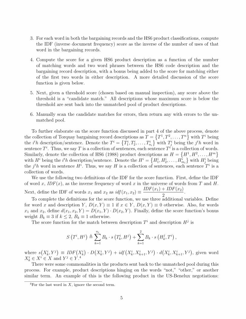
3. For each word in both the bargaining records and the HS6 product classifications, computethe IDF (inverse document frequency) score as the inverse of the number of uses of thatword in the bargaining records.

4. Compute the score for a given HS6 product description as a function of the numberof matching words and two word phrases between the HS6 code description and thebargaining record description, with a bonus being added to the score for matching eitherof the first two words in either description. A more detailed discussion of the scorefunction is given below.

5. Next, given a threshold score (chosen based on manual inspection), any score above thethreshold is a “candidate match.” All descriptions whose maximum score is below thethreshold are sent back into the unmatched pool of product descriptions.

6. Manually scan the candidate matches for errors, then return any with errors to the un-matched pool.

To further elaborate on the score function discussed in part 4 of the above process, denotethe collection of Torquay bargaining record descriptions as T =

{T 1, T 2, . . . , T n

}with T i being

the ith description/sentence. Denote the T i ={T i1, T

i2, . . . , T

ini

}with T i

j being the jth word insentence T i. Thus, we say T is a collection of sentences, each sentence T i is a collection of words.Similarly, denote the collection of HS6 (1988) product descriptions as H =

{H1, H2, . . . , Hm

}with H i being the ith description/sentence. Denote the H i =

{H i

1, Hi2, . . . , H

imi

}with H i

j beingthe jth word in sentence H i. Thus, we say H is a collection of sentences, each sentence T i is acollection of words.

We use the following two definitions of the IDF for the score function. First, define the IDFof word x, IDF (x), as the inverse frequency of word x in the universe of words from T and H.

Next, define the IDF of words x1 and x2 as idf (x1, x2) ≡IDF (x1) + IDF (x2)

2.

To complete the definitions for the score function, we use three additional variables. Definefor word x and description Y , D(x, Y ) ≡ 1 if x ∈ Y , D(x, Y ) ≡ 0 otherwise. Also, for wordsx1 and x2, define d(x1, x2, Y ) = D(x1, Y ) ·D(x2, Y ). Finally, define the score function’s bonusweight Bk ≡ 3 if k ≤ 2, Bk ≡ 1 otherwise.

The score function for the match between description T i and description Hj is

S(T i, Hj

),

ni∑k=1

Bk · s(T ik, H

j)

+2∑

k=1

Bk · s(Hj

k, Ti),

where s(X i

k, Yj)≡ IDF

(X i

k

)· D(X i

k, Yj)

+ idf(X i

k, Xik+1, Y

j)· d(X i

k, Xik+1, Y

j), given word

X ik ∈ X i ∈ X and Y j ∈ Y .4

There were some commonalities in the products sent back to the unmatched pool during thisprocess. For example, product descriptions hinging on the words “not,” “other,” or anothersimilar term. An example of this is the following product in the US-Benelux negotiations:

4For the last word in X, ignore the second term.

5

Ammonium compounds, n.e.s.: Other than ammonium chrome alum. In this case, the matchingalgorithm generated the exact same set of HS6 code matches as the matches generated forAmmonium compounds, n.e.s.: Ammonium chrome alum.

Third Stage. For all remaining unmatched product descriptions, we manually wentthrough each individual product description and assigned HS6 codes. Manual matching re-lied greatly on the use of online HS Code search engines and various other websites, as manyterms used to describe products in the 1948 data are archaic.5

We performed this three-step process on the bargaining records. In the end, we were ableto match 97% of the product entries in the bargaining records to a 1988 HS6 code.

1.3. Aggregation of Bargaining Records

We aggregate the Torquay bargaining data (originally at eight- to ten-digit level with variouscountry codes) up to the HS6 level. Hence, for any HS6 code, we are typically aggregatingmultiple records from the more disaggregated product data.

To aggregate the bargaining data, we do the following: (a) unless otherwise indicated,for variables referring to ad valorem or specific tariff levels (initial, offered, requested), weaggregate the tariff level for HS6 product i as an unweighted average of the tariff levels forthe disaggregated products that have been allocated to HS6 product i (and omit from theaverage any missing disaggregated-product tariff levels); and (b) unless otherwise indicated, fordummy/indicator variables referring to whether an action (e.g., a request from country j onHS6 product i, or a US agreement on HS6 product i) has or has not occurred, we define theaction as occurring for HS6 product i if and only if it occurs for at least one disaggregatedproduct that has been allocated to HS6 product i.

5One of the most useful search engines, the Schedule B Search Engine (created by 3CE Technologies) isavailable at https://uscensus.prod.3ceonline.com.

6