online algorithms for sum-product networks with continuous...
TRANSCRIPT

Online Algorithms for Sum-Product Networks with Continuous Variables
Priyank Jaini
Ph.D. Seminar

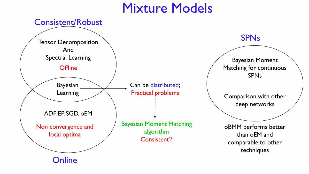
Tensor Decomposition
And
Spectral Learning
Offline
ADF, EP, SGD, oEM
Non convergence and
local optima
Consistent/Robust
Online
Bayesian
Learning
Can be distributed;
Practical problems
Bayesian Moment Matching
algorithm
Bayesian Moment
Matching for continuous
SPNs
Comparison with other
deep networks
SPNs
Mixture Models

Streaming Data
Activity Recognition Recommendation
Challenge : update model after each observation

x1:t
Online
xa:b
xc:d
xa:dDistributed
xt
Θ*
Consistent
Algorithm’s characteristics
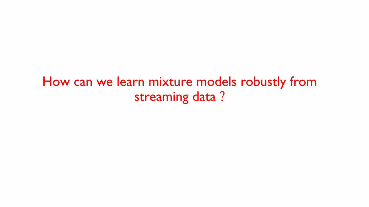
How can we learn mixture models robustly from streaming data ?

Learning Algorithms
• Robust : Tensor Decomposition(Anandkumar et.al,
2014),Spectral Learning(Hsu et al, 2012, Parikar and Xing, 2011);
offline
• Online :
• Assumed Density Filtering (Maybeck 1982; Lauritzen 1992;
Opper & Winther 1999); not robust
• Expectation Propagation (Minka 2001); does not converge
• Stochastic Gradient Descent (Zhang 2004)
• online Expectation Maximization (Cappe 2012)
SGD and oEM : local optimum and cannot be distributed
Learning Algorithms
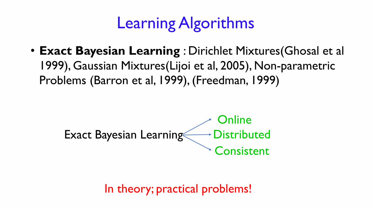
• Exact Bayesian Learning : Dirichlet Mixtures(Ghosal et al
1999), Gaussian Mixtures(Lijoi et al, 2005), Non-parametric
Problems (Barron et al, 1999), (Freedman, 1999)
Exact Bayesian Learning Distributed
Online
Consistent
In theory; practical problems!
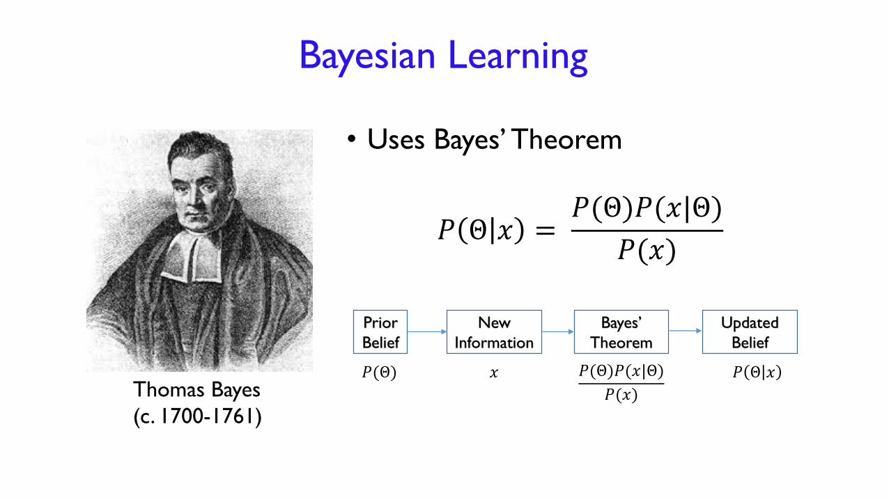
Bayesian Learning
• Uses Bayes’ Theorem
𝑃 Θ 𝑥 =𝑃(Θ)𝑃(𝑥|Θ)
𝑃(𝑥)
Thomas Bayes
(c. 1700-1761)
Prior
Belief
New
Information
Bayes’
Theorem
Updated
Belief
𝑃(Θ) 𝑥 𝑃 Θ 𝑥𝑃(Θ)𝑃(𝑥|Θ)
𝑃(𝑥)
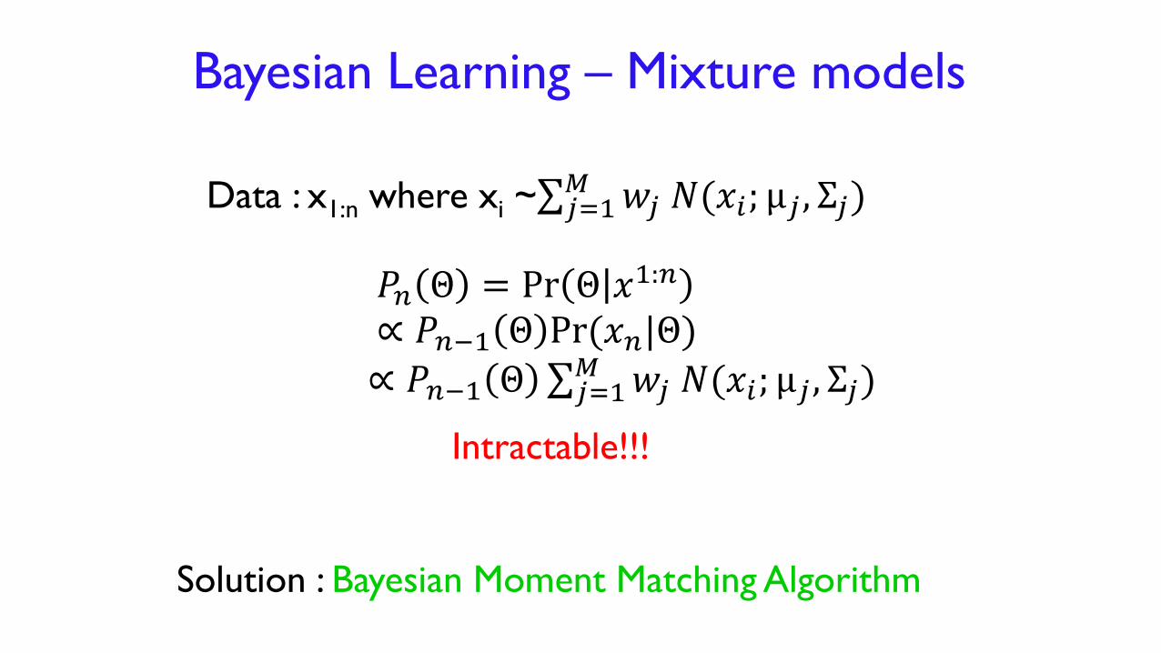
Bayesian Learning – Mixture models
Data : x1:n where xi ~ 𝑗=1𝑀 𝑤𝑗 𝑁(𝑥𝑖; µ𝑗 , Σ𝑗)
𝑃𝑛 Θ = Pr Θ 𝑥1:𝑛
∝ 𝑃𝑛−1 Θ Pr(𝑥𝑛|Θ)
∝ 𝑃𝑛−1 Θ 𝑗=1𝑀 𝑤𝑗 𝑁(𝑥𝑖; µ𝑗 , Σ𝑗)
Intractable!!!
Solution : Bayesian Moment Matching Algorithm
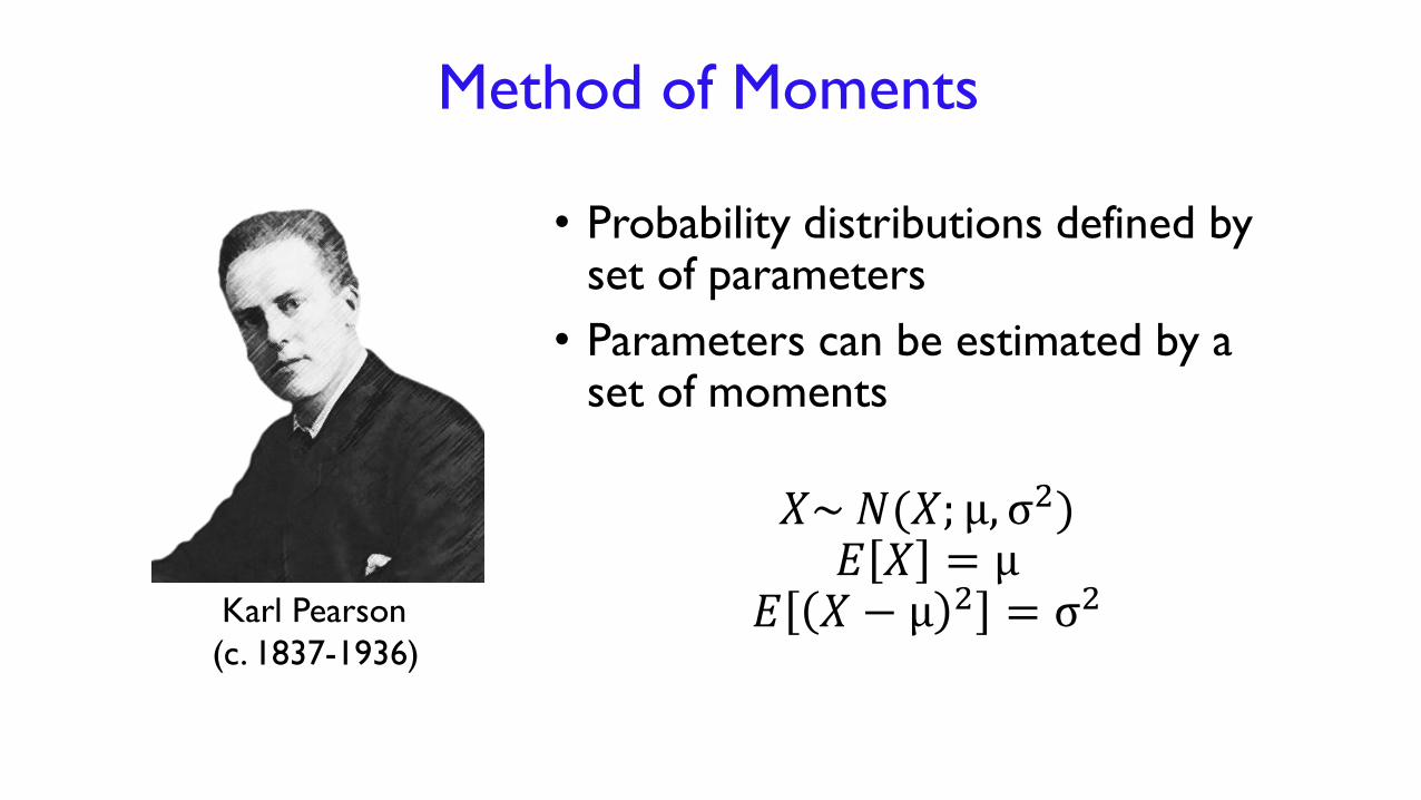
Method of Moments
• Probability distributions defined by set of parameters
• Parameters can be estimated by a set of moments
𝑋~ 𝑁(𝑋; µ, σ2)𝐸 𝑋 = µ
𝐸 𝑋 − µ 2 = σ2Karl Pearson
(c. 1837-1936)

Make Bayesian Learning Great Again
Bayesian Learning
AndMethod of Moments

Gaussian Mixture Models
xi ~ 𝑗=1𝑀 𝑤𝑗 𝑁(𝑥𝑖; µ𝑗 , Σ𝑗)
Parameters : weights,
means and precisions
(inverse covariance matrices)
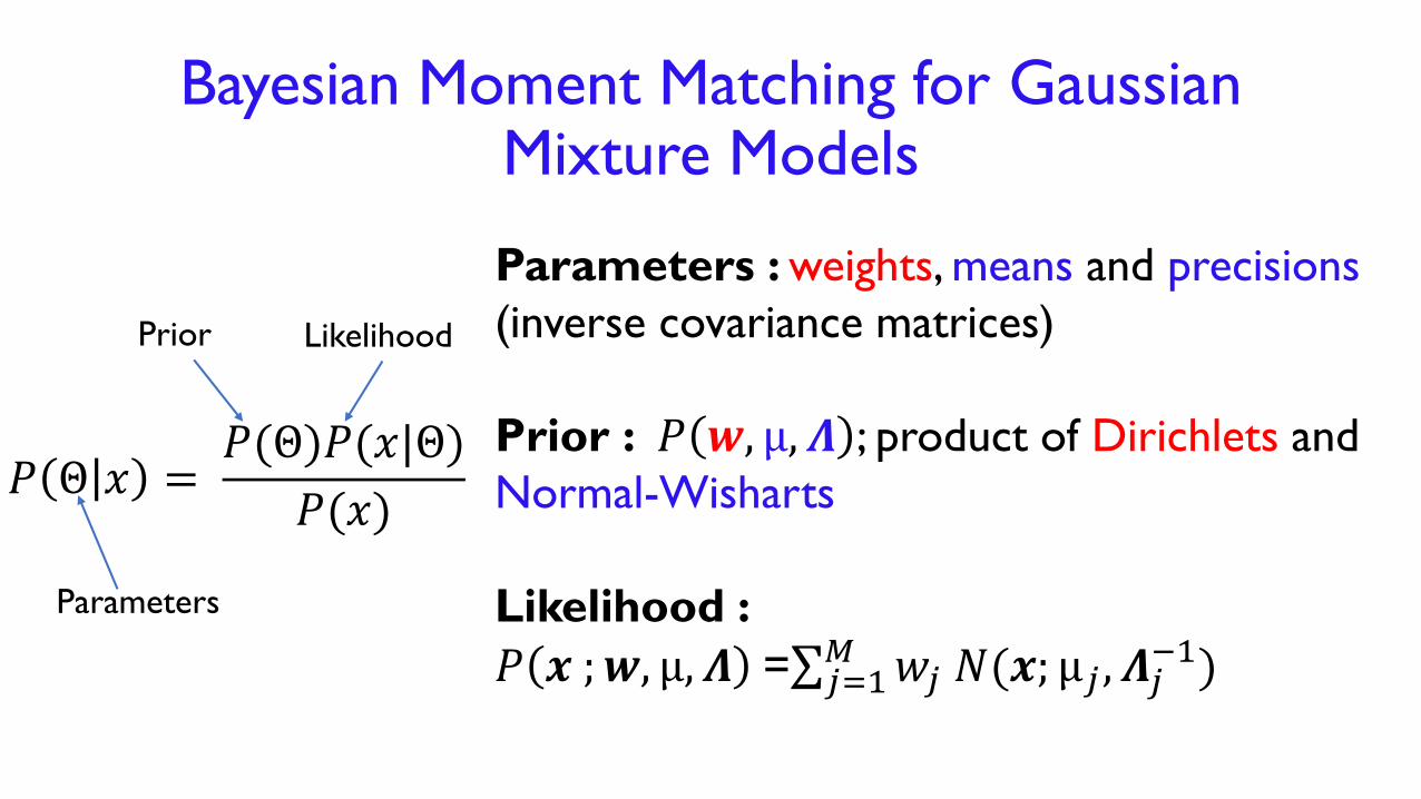
Bayesian Moment Matching for Gaussian Mixture Models
Parameters : weights, means and precisions
(inverse covariance matrices)
Prior : 𝑃 𝒘, µ, 𝜦 ; product of Dirichlets and
Normal-Wisharts
Likelihood :
𝑃 𝒙 ;𝒘, µ, 𝜦 = 𝑗=1𝑀 𝑤𝑗 𝑁(𝒙; µ𝑗 , 𝜦𝑗
−1)
𝑃 Θ 𝑥 =𝑃(Θ)𝑃(𝑥|Θ)
𝑃(𝑥)
Parameters
Prior Likelihood
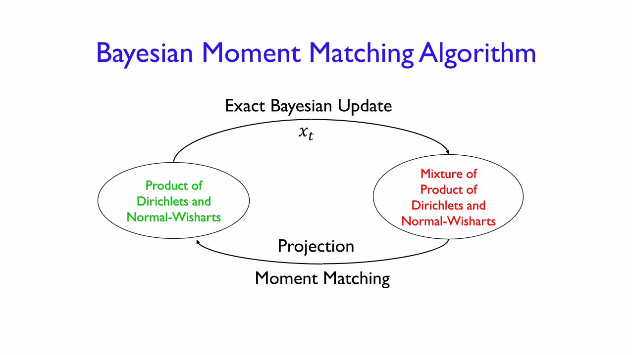
Bayesian Moment Matching Algorithm
Product of
Dirichlets and
Normal-Wisharts
Mixture of
Product of
Dirichlets and
Normal-Wisharts
Exact Bayesian Update
Moment Matching
𝑥𝑡
Projection

Sufficient Moments
Dirichlet : 𝐷𝑖𝑟 𝑤1, 𝑤2…𝑤𝑀; α1, α2… , α𝑀
𝐸 𝑤𝑖 =α𝑖
𝑗 α𝑗; 𝐸 𝑤𝑖
2 =α𝑖(α𝑖+1)
( 𝑗 α𝑗)(1+ 𝑗 α𝑗)
Normal-Wishart : 𝑁𝑊 µ, 𝛬 ; µ0, κ,𝑊, 𝑣𝛬 ~ Wi(𝑊,𝑣) and µ|𝛬 ~ 𝑁𝑑 µ0, 𝜅𝛬
−1
𝐸 µ = µ0𝐸 (µ − µ0)(µ − µ0)
𝑇 =κ+1
κ(𝑣−𝑑−1)𝑊−1
𝐸 𝛬 = 𝑣𝑊
𝑉𝑎𝑟 𝛬𝑖𝑗 = 𝑣(𝑊𝑖𝑗2 +𝑊𝑖𝑖𝑊𝑗𝑗)
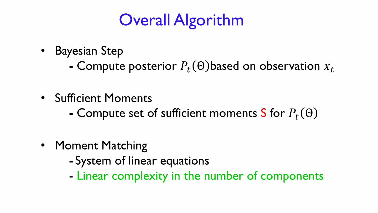
Overall Algorithm
• Bayesian Step
- Compute posterior 𝑃𝑡 Θ based on observation 𝑥𝑡
• Sufficient Moments
- Compute set of sufficient moments S for 𝑃𝑡 Θ
• Moment Matching
- System of linear equations
- Linear complexity in the number of components

Make Bayesian Learning Great Again
Bayesian Moment Matching Algorithm
- Uses Bayes’ Theorem + Method of Moments
- Analytic solutions to Moment matching (unlike EP, ADF)
- One pass over data
Bayesian Moment Matching Distributed
Online
Consistent ?

Experiments
Data Set Instances oEM oBMM
Abalone 4177 -2.65 -1.82
Banknote 1372 -9.74 -9.65
Airfoil 1503 -15.86 -16.53
Arabic 8800 -15.83 -14.99
Transfusion 748 -13.26 -13.09
CCPP 9568 -16.53 -16.51
Comp. Ac 8192 -132.04 -118.82
Kinematics 8192 -10.37 -10.32
Northridge 2929 -18.31 -17.97
Plastic 1650 -9.46 -9.01

Experiments
Data (Features) Instances oEM oBMM oDMM
Heterogeneity(16) 3,930,257 -176.2 -174.3 -180.7
Magic (10) 19,000 -33.4 -32.1 -35.4
Year MSD (91) 515,345 -513.7 -506.5 -513.8
Miniboone (50) 130,064 -58.1 -54.7 -60.3
Data (Features) Instances oEM oBMM oDMM
Heterogeneity(16) 3,930,257 77.3 81.7 17.5
Magic (10) 19,000 7.3 6.8 1.4
Year MSD (91) 515,345 336.5 108.2 21.2
Miniboone (50) 130,064 48.6 12.1 2.3
Running Time
Avg. Log-Likelihood
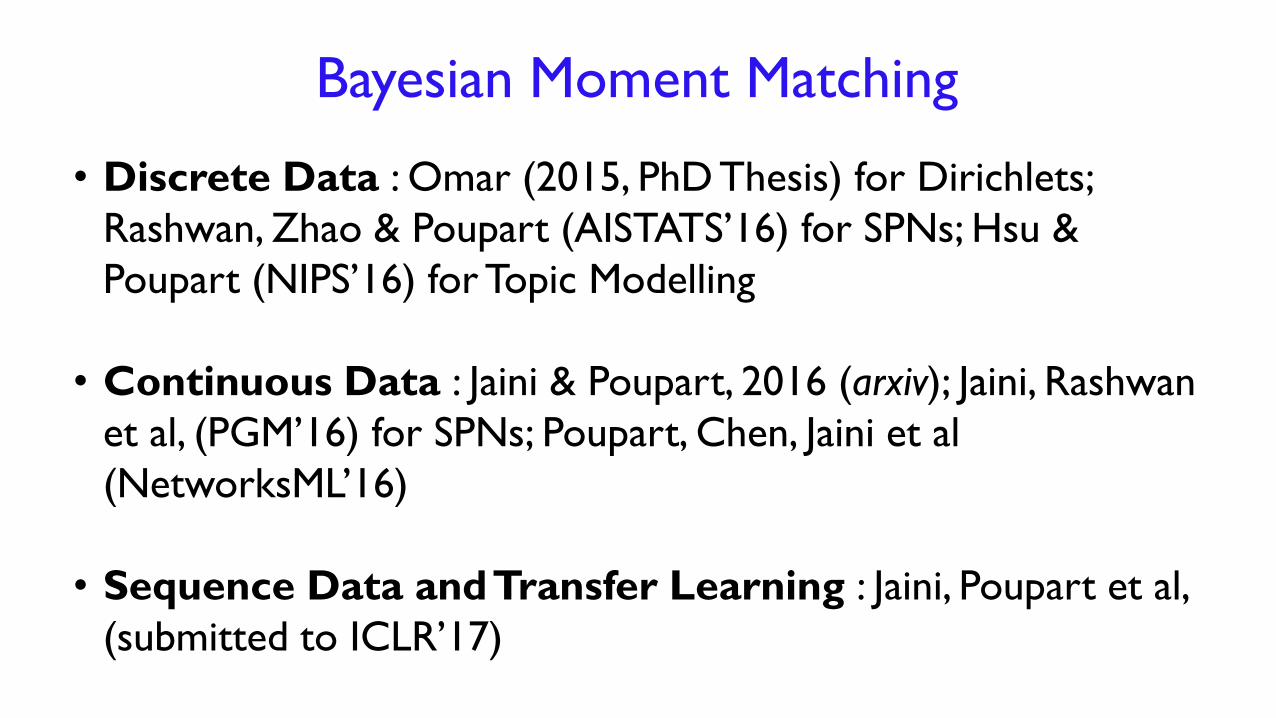
Bayesian Moment Matching
• Discrete Data : Omar (2015, PhD Thesis) for Dirichlets;
Rashwan, Zhao & Poupart (AISTATS’16) for SPNs; Hsu &
Poupart (NIPS’16) for Topic Modelling
• Continuous Data : Jaini & Poupart, 2016 (arxiv); Jaini, Rashwan
et al, (PGM’16) for SPNs; Poupart, Chen, Jaini et al
(NetworksML’16)
• Sequence Data and Transfer Learning : Jaini, Poupart et al,
(submitted to ICLR’17)

Tensor Decomposition
And
Spectral Learning
Offline
ADF, EP, SGD, oEM
Non convergence and
local optima
Consistent/Robust
Online
Bayesian
Learning
Can be distributed;
Practical problems
Bayesian Moment Matching
algorithm
Consistent?
Bayesian Moment
Matching for continuous
SPNs
Comparison with other
deep networks
SPNs
Mixture Models

What is a Sum-Product Network?
Proposed by Poon and Domingos (UAI 2011)
equivalent to Arithmetic Circuits (Darwiche 2003)
Deep architecture
with clear
semantics
Tractable
Probabilistic
Graphical Models
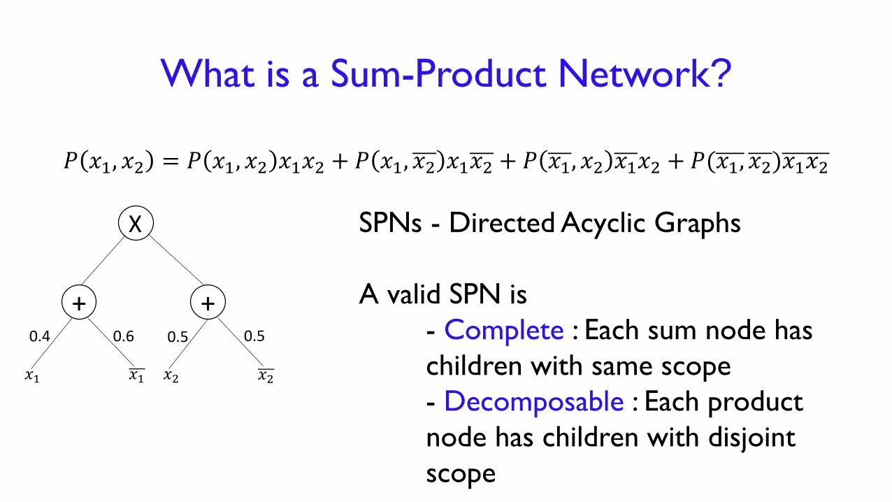
What is a Sum-Product Network?
𝑃 𝑥1, 𝑥2 = 𝑃 𝑥1, 𝑥2 𝑥1𝑥2 + 𝑃 𝑥1, 𝑥2 𝑥1𝑥2 + 𝑃 𝑥1, 𝑥2 𝑥1𝑥2 + 𝑃(𝑥1, 𝑥2)𝑥1𝑥2
ax
++
𝑥1 𝑥2 𝑥2𝑥1
X
0.4 0.50.6 0.5
SPNs - Directed Acyclic Graphs
A valid SPN is
- Complete : Each sum node has
children with same scope
- Decomposable : Each product
node has children with disjoint
scope

Probabilistic Inference - SPN
SPN represents a joint distribution over a
set of random variables
Example :
Query : Pr(𝑋1 = 1, 𝑋2 = 0)
𝑃𝑟(𝑋1 = 1, 𝑋2 = 0) = 34.8/100
Linear Complexity – two bottom passes
for any query
1 1 1 1
10 10 10
100 100
100
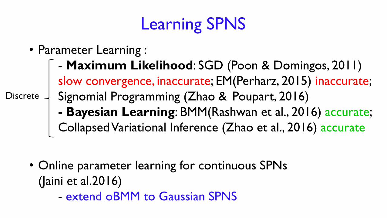
Learning SPNS
• Parameter Learning :
- Maximum Likelihood: SGD (Poon & Domingos, 2011)
slow convergence, inaccurate; EM(Perharz, 2015) inaccurate;
Signomial Programming (Zhao & Poupart, 2016)
- Bayesian Learning: BMM(Rashwan et al., 2016) accurate;
Collapsed Variational Inference (Zhao et al., 2016) accurate
Discrete
• Online parameter learning for continuous SPNs
(Jaini et al.2016)
- extend oBMM to Gaussian SPNS

Continuous SPNS
𝑁1(𝑋1) 𝑁2(𝑋1) 𝑁3(𝑋2) 𝑁4(𝑋2)𝑁1(𝑋1)
Gaussian
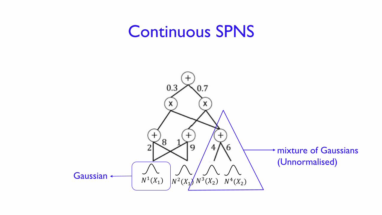
Continuous SPNS
𝑁1(𝑋1) 𝑁2(𝑋1) 𝑁3(𝑋2) 𝑁4(𝑋2)𝑁1(𝑋1)
Gaussian
mixture of Gaussians
(Unnormalised)

Continuous SPNS
𝑁1(𝑋1) 𝑁2(𝑋1) 𝑁3(𝑋2) 𝑁4(𝑋2)
Hierarchical mixture of Gaussians
(Unnormalised)

Bayesian Learning of SPNs
+ +
+
+
+
+
N(𝑋1; µ1, Λ1−1 )N(𝑋1; µ2, Λ2
−1 )
N(𝑋2; µ3, Λ3−1 ) N(𝑋2; µ4, Λ4
−1 )𝑤1
𝑤2 𝑤3 𝑤4𝑤5 𝑤6
𝑤7 𝑤8
Parameters : weights, means and
precisions (inverse covariance matrices)
Prior : 𝑃 𝒘, µ, 𝜦 ; product of Dirichlets
and Normal-Wisharts
Likelihood :
𝑃 𝒙 ;𝒘, µ, 𝜦 =S𝑃𝑁 𝒙 ;𝒘, µ, 𝜦
Posterior :
𝑃 𝒘, µ, 𝜦; 𝒅𝒂𝒕𝒂 ∝𝑃 𝒘, µ, 𝜦 𝒏 S𝑃𝑁 𝒙𝒏 ; 𝒘, µ, 𝜦

Bayesian Moment Matching Algorithm
Product of
Dirichlets and
Normal-Wisharts
Mixture of
Product of
Dirichlets and
Normal-Wisharts
Exact Bayesian Update
Moment Matching
𝑥𝑡
Projection
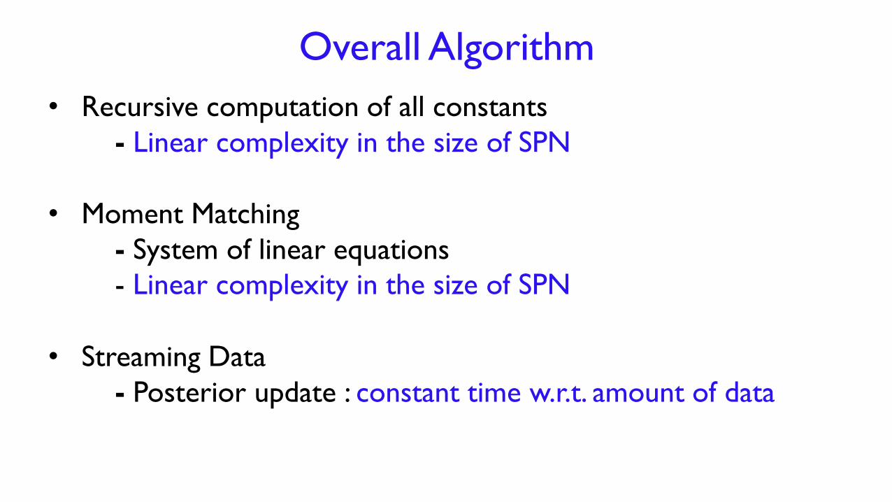
Overall Algorithm
• Recursive computation of all constants
- Linear complexity in the size of SPN
• Moment Matching
- System of linear equations
- Linear complexity in the size of SPN
• Streaming Data
- Posterior update : constant time w.r.t. amount of data

Empirical Results
Dataset Flow Size Quake Banknote Abalone Kinematics CA Sensorless
Drive
Attributes 3 4 4 8 8 22 48
oBMM
(random)
- - - -1.82 ∓0.19
-11.19∓0.03
-2.47 ∓0.56
1.58 ∓1.28
oEM
(random)
- - - -11.36 ∓0.19
-11.35 ∓0.03
-31.34 ∓1.07
-3.40 ∓6.06
oBMM
(GMM)
4.80 ∓0.67
-3.84 ∓0.16
-4.81 ∓0.13
-1.21∓0.36
-11.24 ∓0.04
-1.78 ∓0.59
-
oEM
(GMM)
-0.49 ∓3.29
-5.50 ∓0.41
-4.81 ∓0.13
-3.53 ∓1.68
-11.35 ∓0.03
-21.39 ∓1.58
-
Avg. log-likelihood and standard error based on 10-fold cross-validation
oBMM performs better than oEM
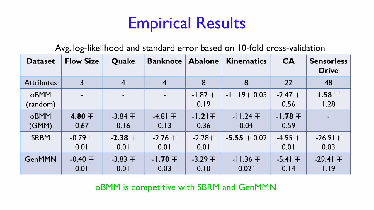
Empirical Results
Dataset Flow Size Quake Banknote Abalone Kinematics CA Sensorless
Drive
Attributes 3 4 4 8 8 22 48
oBMM
(random)
- - - -1.82 ∓0.19
-11.19∓ 0.03 -2.47 ∓0.56
1.58 ∓1.28
oBMM
(GMM)
4.80 ∓0.67
-3.84 ∓0.16
-4.81 ∓0.13
-1.21∓0.36
-11.24 ∓0.04
-1.78 ∓0.59
-
SRBM -0.79 ∓0.01
-2.38 ∓0.01
-2.76 ∓0.01
-2.28∓0.01
-5.55 ∓ 0.02 -4.95 ∓0.01
-26.91∓0.03
GenMMN -0.40 ∓0.01
-3.83 ∓0.01
-1.70 ∓0.03
-3.29 ∓0.10
-11.36 ∓0.02`
-5.41 ∓0.14
-29.41 ∓1.19
Avg. log-likelihood and standard error based on 10-fold cross-validation
oBMM is competitive with SBRM and GenMMN
Tensor Decomposition
And
Spectral Learning
Offline
ADF, EP, SGD, oEM
Non convergence and
local optima
Consistent/Robust
Online
Bayesian
Learning
Can be distributed;
Practical problems
Bayesian Moment Matching
algorithm
Consistent?
Bayesian Moment
Matching for continuous
SPNs
Comparison with other
deep networks
SPNs
Mixture Models
oBMM performs better
than oEM and
comparable to other
techniques
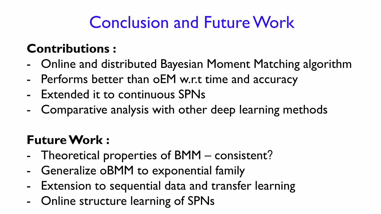
Conclusion and Future Work
Contributions :
- Online and distributed Bayesian Moment Matching algorithm
- Performs better than oEM w.r.t time and accuracy
- Extended it to continuous SPNs
- Comparative analysis with other deep learning methods
Future Work :
- Theoretical properties of BMM – consistent?
- Generalize oBMM to exponential family
- Extension to sequential data and transfer learning
- Online structure learning of SPNs

Thank you!