ongeneralizationofadditivemaineﬀectand ...einspem.upm.edu.my/journal/fullpaper/vol11sfeb/8. alfian...

Malaysian Journal of Mathematical Sciences 11(S) February: 115–141 (2017)Special Issue: Conference on Agriculture Statistics 2015 (CAS 2015)

MALAYSIAN JOURNAL OF MATHEMATICAL SCIENCES

Journal homepage: http://einspem.upm.edu.my/journal

On Generalization of Additive Main Effect andMultiplicative Interaction (AMMI) Models: AnApproach of Row Column Interaction Models for

Counting Data

Hadi, A. F. ∗1, Sa’diyah, H. 2, and Iswanto, R. 3

1Statistical Laboratory, Department of Mathematics, University ofJember, Indonesia

2Biometrics Laboratory, Department of Agronomy, University ofJember, Indonesia

3Indonesian Legumes and Tuber Crops Research Institute,Indonesia

E-mail: [email protected]∗Corresponding author

ABSTRACT

Additive Main Effect and Multiplicative Interaction (AMMI) model wascommonly used to analyze Genotype Environment × Interaction withnormal response variables, now it had been generalized for categorical orother non-normal response variables, called GAMMI model. This devel-opment was conducted by introducing multiplicative terms to the Gen-eralized Linear Model (GLM). This research round up our previous workon developing an approach of Row Column Interaction Models (RCIMs)comprise to GAMMI model and focus to get more generalized for count-ing data with overdispersed and zeros problems. A few interesting thingshere are (i) an issue of distribution on GLM sense and (ii) an issue ofmodel’s complexity that is the number of multiplicative terms to fit theinteraction effect more properly. On the distribution issue of countingdata, we will focus on Poisson, Negative Binomial (NB), and zero inflatedproblems with Zero Inflated Poisson (ZIP) and Zero Inflated NB (ZINB)

Hadi, A. F., Sa’diyah, H. and Iswanto, R.

distribution. A simulation conducted by adding outlier(s) on a Poissoncounting data for overdispersed condition, and adding zeros observationon the data for illustrating the zero problems. We propose the NB modelfor overdispersed data and model of ZIP or ZINB for data with both,overdispersed and zero problem. In the case of both illnesses conditionshappened simultaneously, the mean square error of NB and ZINB will in-crease slightly. But the ZINB was resulting the simplest model of RCIMwith less number of interaction terms.

Keywords: Multiplicative Models, Negative Binomial, Overdisperse, Pois-son, Zero Inflated.

116 Malaysian Journal of Mathematical Sciences

On Generalization of AMMI Models: An Approach of RCIM for Counting Data

1. Introduction

AMMI model is commonly used to analyze stability and adaptability onthe Genotype × Environments interaction (GEI) studies. AMMI provide anadditive model for main effects of genotype and environment plus a completemultiplicative terms for the interaction effects. Basically, the interaction termswas modeled by a statistical technique of reduction dimension called Singu-lar Value Decomposition (SVD). With SVD, the interaction terms will havecomplete parameters, a paramater for every single cell of the two ways table.SVD will visualize the interaction terms by Biplot and makes the GEI analysisbecome easier. With this feature of Biplot, AMMI said to be most powerfulmodel for the GEI (Hadi et al. (2010)).

The advantages of AMMI model for the GEI analysis, together with it’s limi-tation on normality assumption, inspire many statisticians to develop AMMI tobe more generalized by introducing GLM sense to AMMI model. Van Eeuwijk(1995) propose the Generalized AMMI model which introduce multiplicativeterm to GLM. GAMMI also keep the feature of Biplot visualization of GEI.Nowadays, GAMMI model had been broadly applied to a counting data res-ponse as in Hadi et al. (2010). Another overlapping methodology is the RCIMof Yee and Hadi (2014). RCIM is designed for many kind of interaction modelwith various response including GAMMI for Poisson count. In case of Poissonresponse in two ways table, formula of RCIM look identical to GAMMI modelwith log-link function. RCIM was an approach built up on Reduce Rank Re-gression (RRR) for GLM, it’s called RR-VGLM (Yee and Hastie (2003)) whileGAMMI used a criss-cross regression (Van Eeuwijk (1995)). Computation ofparameter estimate of these two models used the same type of algorithm ofalternating regression, it was confirmed by Turner and Firth (2015) and alsoby Yee and Hadi (2014). In spite of this similarity, they are different in modelparameterization and constraint, thus it still allows them to give different re-sult.

Starting with a framework of statistical development of RCIM as an alter-native model to GAMMI for two ways table of counting data, this paper wantto deliver a wrap up review of our previous work on application of RCIM toGEI analysis, and to get more generalized of GAMMI model by an approachof RCIM model. We focus on the generalization for counting data related tothe limitation problematic of equidispersion assumption of Poisson distribu-tion (that the conditional means of Poisson data distributed is equal to it’svariance). With this strict assumption of Poisson, any extreme values of ob-servation may cause a violation of the pure Poisson distribution. The mainviolation here is the overdispersion, when a counting data has variance greater

Malaysian Journal of Mathematical Sciences 117


than the mean is called overdispersed. A Poisson data distributed with largemean value will also has a large variance, thus any large extreme value (rightoutlier) will be interesting here. On the other hand, any extreme value(s) hereis including a zero valued observation(s). Poisson with a low mean valued mayhave extra-zero observations, then here Poisson will mimic a problem called anextra-zero or a zero-inflation problem.

We found a few interesting issues. The first issue is the data distribution,about the canonical link function applied on GLM to fit the data properly.Here, we focus on Poisson and NB distribution, including problems of overdis-persion by outliers and also zero-inflation with ZIP and ZINB distribution. Thesecond issue is the model’s complexity. It is about the number of multiplicativeterms involved in the model (represented by rank of model) to describe the in-teraction effects. A simple scheme of simulation was conducted to present anoverdispersion and zero-inflated condition into a Poisson counting data. Thenwe introduce RCIM with NB distribution for handling overdispersed data countby outliers, also ZIP and ZINB for zero-inflated problem.

2. Row Column Interaction Models (RCIM)

This section will discuss a framework of developing model of RCIM (Figure1). RCIM will fit data count of two ways table with every single cell containingrow and column effects plus some interaction effects as reduce rank regressionand visualize the interaction terms of rank = 2 by biplot. Here RCIM was verysimilar to GAMMI model, where GAMMI was decomposing the interactioneffects by Singular Value Decomposition (SVD) and also visualize it throughbiplot for the first two singular vectors. Both approaches give similar results,differing only in numerical computation aspect and no statistically essential.Yee and Hadi (2014) said that RCIM is developed from RR-VGLM which isapplied to a matrix data of row-column containing interaction effects by reducerank regression. RR-VGLM it self is a variant of Vector GLM (VGLM), asclearly described in Yee and Hastie (2003). For further reading, there were someearly discussions of RR-VGLM in RCIM context such as Yee and Hadi (2014)and Hadi and Sa’diyah (2016), we also can find for more wider class of modelingin Yee (2015). Something important here, that is the compliance of parametersetting in RR-VGLM. We turn it to the SVD parameterization, and we willdepart to develop RCIM for two way table that comprise to GAMMI model forthe GEI. The RCIMs approach for GEI analysis has introduce an applicativebiplot visualization of the interaction effects in case of Poisson counting dataresponse with zero-inflated problems (Hadi and Sa’diyah (2014)). Later, Hadiand Sa’diyah (2016) was supplementing RCIM as alternative way to GAMMI



model with the deviance analysis for determining the number of multiplicativeterms needed for the interaction analysis or even for handling overdispersion,both at once. Furthermore, we now will develop RCIM to be more generalizedwith Negative Binomial and also Zero Inflated Negative Binomial.

, log

1

R

k

jkikjiij c

𝜼𝟏𝒊𝒋 = 𝝁 + 𝜶𝒊 + 𝜸𝒋 + 𝒂𝒊𝒌𝒄𝒋𝒌𝑹𝒌=𝟏

Figure 1: Statistical framework of The RCIM

2.1 VGLMs and RR-VGLMs

RCIM was built upon VGLMs and RR-VGLMs (see Figure 1). We nowgenerally, will talk about VGLMs and RR-VGLMs, for more detail the readerdirected to see Yee and Hastie (2003), Yee (2014) and also Yee (2015). Let theobserved response y is a q-dimensional vector. VGLMs are defined as a modelwhere

f(y|x;B) = h(y, η1, . . . , ηM ) (1)



for some known function h(·), B = (β1 β2 · · · βM ) is a p×M matrix of unknownregression coefficients and x is explanatory. The jth linear predictor is

ηj = βTj x =

p∑k=1

β(j)k xk, j = 1, . . . ,M, (2)

where x = (x1, . . . , xp)T with x1 = 1 for an intercept.

GLMs only have single linear predictor of η for the mean, but VGLMs mayhave more, each may be applied to a certain parameters of a distribution. Forexample, a univariate distribution has two parameters of the location parame-ter a and the scale parameter b. Then we might take two linear predictors ofVGLM here, η1 is for a and η2 is for b. In general, ηj = gj(θj) for some certainlink function gj and parameter θj . VGAM offers many link functions, thatcan be assigned to any parameters, ensuring maximum flexibility.

Most VGLMs have a log-likelihood which is maximized. Let xi denote theexplanatory vector for the ith observation, for i = 1, . . . , n. Then we can writethe equation 2 as

ηi =

η1(xi)...

ηM (xi)

= BTxi =

βT1 xi...

βTMxi

. (3)

The IRLS algorithm behind VGAM almost always implements Fisher scoringbased on the expected information matrix (EIM) at the individual i level.

In practice we may wish to constrain the effect of a covariate to be the samefor some of the ηj and to have no effect for others. For example,

η1 = β∗(1)1 + β∗(1)2 x2 + β∗(1)3 x3,

η2 = β∗(2)1 + β∗(1)2 x2,

so that β(1)2 ≡ β(2)2 and β(2)3 ≡ 0. The star superscript denote regressionparameters that are actually estimated. For VGLMs, we can represent thesemodels using

η(x) =

p∑k=1

β(k) xk =

p∑k=1

Hk β∗(k) xk (4)

where H1,H2, . . . ,Hp are known full-column rank constraint matrices, β∗(k) isa vector containing a possibly reduced set of regression coefficients. With noconstraint at all, all Hk = IM and β∗(k) = β(k). Then

BT =(H1β

∗(1) H2β

∗(2) · · · Hpβ

∗(p)

). (5)



2.1.1 The RR-VGLMs

Represent the VGLMs of (1) and its linear predictor of (2), we now turnto partition x into (xT1 , x

T2 )T and B = (BT

1 BT2 )T . In general, B is a full rank

matrix of min(M,p). There are M × p regression coefficients to be estimated.In some cases, it would be a problem here like degree of freedom deficiencies orother problems regarding that is too many parameters to be estimated. Nowwe need a method of dimension reduction here. That is to replace B2 by anRRR of B2 = ACT with lower rank of R ≤ min(M,p) matrices of A andC. This reduction of the number of regression coefficients will done efficientlyby put R as low, e.g., 0 or 1 or 2. Something grab our attention for the nextfeature of our model. That is a fact that by taking R = 2, the A and C maybe biplotted. The reduced-rank regression is applied to B2 because we want tomake provision the variables in x1 to be left alone for the intercepts.

Now we have the RR-VGLMs of the form

η = BT1 x1 + BT

2 x2 = BT1 x1 + ACTx2 = BT

1 x1 + A ν (6)

where C = (c(1) · · · c(R)) is p2 × R, A = (a(1) · · · a(R)) = (a1, . . . , aM )T isM × R. Both A and C are of full-column rank. Of course, R ≤ min(M,p2)but ideally we want R � min(M,p2). One can think of (6) as a reduced-rankregression of the coefficients of x2 after having adjusted for the variables in x1(commonly x1 is left as the intecept of µ).

In order to make the parameter being unique, we may enforce identifiabilityconstraint to restrict A to the form

A =

(IR

A

), say, (7)

called corner constraints. Actually, it may be necessary to represent IR inrows other than the first R; this is controlled by the argument Index.cornerwhich has value 1:Rank as default. It transpires that RR-VGLMs are VGLMswhere the constraint matrices are estimated. An alternating algorithm is usedwhich toggles between estimating A and C one at a time based on the currentestimate of the other.



2.2 Row-Column Interaction Model for Data count in theRR-VGLM

2.2.1 Goodman’s Row-Column association model

Hadi and Sa’diyah (2014) use an association model of Goodman’s Row-Column (GRC) of Goodman (1981) to describe the RCIM model in the RR-VGLMs framework, by firstly assuming that Y = [(yij)] is a n ×M matrixof counts and Yij has a Poisson distribution, E(Yij) = µij is the mean of thei-j cell. Goodman’s RC(R) association model fits a reduced-rank type modelto Y, and the linear predictor is

log µij = µ+ αi + γj +

R∑r=1

cir ajr, (8)

where i = 1, . . . , n, j = 1, . . . ,M . Note that (8) is saturated when R =min(n,M).

In (8) the parameters αi and γj are called the row and column scores (oreffects) respectively. Identifiability constraints are needed for these, such ascorner constraints, e.g., α1 = γ1 = 0. The parameters air and cjr also needconstraints, e.g., a1r = c1r = 0 for r = 1, . . . , R.

We can write (8) as

log µij = µ+ αi + γj + δij ,

where the n ×M matrix ∆ = [(δij)] of interaction terms is approximated bythe reduced rank quantity

δij =

R∑r=1

cir ajr. (9)

The GRC association model fits within the VGLM framework of (6) byletting

ηi = log µi (10)

where µTi is the mean of the ith row of Y. Then the GRC model will fit thematrix (η1, . . . , ηn)T using RRR by setting up the indicator variables in BT

1 x1i.The reader directed to Yee and Hadi (2014) and Yee (2015) for further readingabout how to get the appropriate indicator variable setting. Similarly, B2 is



approximated by CAT , the ∆ is approximated by x21...x2n

CAT

The desired reduced-rank approximation of ∆ can be obtained if x2i = ei sothat Ip2CAT = CAT . Note that

∆ =

(0 0T

0 ∆

)≈ CAT

=

(0T

C(−1)

)(0(A(−1)

)T ), (11)

that is, the first row of A consists of structural zeros which are ‘omitted’ fromthe reduced rank regression of ∆ (Yee and Hastie (2003)).

2.2.2 The RCIMs, GAMMI models, and SVD reparametriation

Finally, we define RCIMs as a RR-VGLM with

η1ij = µ+ αi + γj +

R∑r=1

cir ajr, (12)

Note that (12) applied to the first linear/additive predictor; for models withM >1 one can leave η2, . . . , ηM unchanged. Of course, choosing η1 for (12) is onlyfor convenience and is the default.

GAMMI model of Van Eeuwijk (1995) as described in Turner and Firth(2015), use the singular value to factor out a measurement of the strength ofinteraction between the row and column scores corresponding to each multi-plicative component. It is indicating the importance of the component, or axis.For cell means µij a GAMMI-R model has the form

g(µij) = αi + βj +

R∑k=1

σkγkiδkj (13)

Based on (13) GAMMI model appear to be identical to RCIMs. Here GAMMIapply a SVD to the ACT , and also some constraints of

∑∀i αi =

∑∀i γi = 0,

the parameters air and cjr use constraints of∑∀i a1r =

∑∀i c1r = 0 for

r = 1, . . . , R (Van Eeuwijk (1995)). While in RCIMs, the interaction termuses corner constraints. The advantage of RCIMs is that it should work



for any VGAM family functions, thus the family size is much bigger (Yeeand Hadi (2014), Yee (2010), Yee (2008)). It is easy to perform some post-transformations such as applying a function of svd() to the VGAM output toobtain the SVD parameterization for GAMMI model (Yee and Hadi (2014)).Now we can see that GAMMI is an RCIMs with some other parameterizationof SVD related to what described in Yee and Hastie (2003).

3. Material and Methods

This research use three datasets which are originally obtained from the ex-perimental trial conducted by Indonesian Legumes and Tuber Crops ResearchInstitute (ILETRI), Malang, Indonesia. The first dataset comes from the ex-perimental trial of study the endurance of five genotypes of soybean to 5 typesof its leaf pests. The second dataset comes from a study of leaf disease at-tack on mung bean. The experimental trial involved 12 genotypes (varieties)of mung bean which planted in 5 different environments at Probolinggo, Jom-bang, Jember, Rasanae, and Bolo. The third dataset obtained from a study ofsoybean in ILETRI. This experiment uses 15 types of soybean lines grown at8 locations with a number of soybean pods. This is a counting data withoutoutlier neither zero observation, which is presented in the form of a matrix witha size of 15 × 8.

3.1 Methodology

We will use the 1st dataset of Poisson distributed to summarize our develop-ment of deviance analysis feature of RCIM to determine the rank of model foranalyzing the interaction terms as provided by GAMMI. A biplot of the inter-action analysis was also provided by RCIM. A study of outlier, overdispersion,and the NB model will be discussed by conducted a scheme of simulation onthe 3rd dataset to make an illness condition of overdispersion by outliers. Weimpose the outliers of about 20 percent cells of 15 × 8 cells data matrix. Withthis simulated dataset, we investigate the influence outliers to the estimatedvalue of dispersion parameter in a standard Poisson model. We also discussabout the use of NB distributional with its canonical link-function to overcomethe overdispersion compared to the standard Poisson model with more inter-action terms in the model. We compare the log-likelihood and also the MSE ofthe Poisson and NB models. In addition we investigate the influence of the per-centages of outliers to the MSE of Poisson and NB models by setting incrementof 0.8%, 1.7%, 2.5%, . . . , 19.2% of outliers in 15 × 8 cells data matrix.



We discuss the zero problem in RCIM by firstly summarize our previousdevelopment of introduce the ZIP distribution to our RCIM model, and applyZIP RCIM to the 2nd dataset also comparing to standard Poisson one by it’slog-likelihood value. Next, we introduce a ZINB distribution on RCIM, andconduct a scheme of simulation to add three zeros into the 3rd dataset byreplacing the three smallest value observations at every column by zeros. Here,we got a lot of zeros on the 3rd dataset and we compare the MSE of the NBand the ZINB. For both illnesses condition of outliers and zeros in one dataset,we replace the maximum value by the outlier, and the smallest three valuesby zeros simultaneously into the 3rd dataset. Again, we compare the MSE ofthe NB and ZINB model. Last, we compare the NB and ZINB for a data withstructural zero as we got in 2nd dataset. We also add outlier(s) by replacingthe maximum value observation at every column by a value of max(column)+ 3 × stdev(column). So we compare the MSE of NB and ZINB to the datawith structural zeros and also outliers at once.

4. Result and Discussion

4.1 An Application of RCIM for GAMMI Models: TheDeviance Analysis and Biplot of RCIM

The first dataset Table (1) contain the population count of 5 types of leafpest on four soybean genotypes. It was originally analyzed by Hadi et al. (2010)on the Poisson distribution with the GAMMI model proposed by Van Eeuwijk(1995).

Table 1: The 1st dataset: Count of population of Leaf Pests on some Soybean Genotypes

Leaf PestsGenotype Bemisia Empooascan Agromyza Lamprosema Longitarsus

tabacci sp. phaseoli indicata suturellinusAC100 2 7 9 2 7IAC80 12 11 4 7 13W80 14 12 5 8 8Wilis 16 12 4 7 16

The deviance for a model of µ is defined as the ratio the likelihood of thesaturated model L(y; y) denumerated by the likelihood of the particular modelL(µ; y) (Pawitan (2001)):

D = 2 logL(y; y)

L(µ; y)(14)



It measures the distance between a particular model µ and the observeddata y. Deviance is also commonly used to compare the two nested modelswith different rank. Suppose we have two models, model A with µA have X1β1of rank p and model B with µB have X1β1 + X2β2 with rank of q, for p lessthan q. The difference in the observed deviance

D(y, µA)−D(y, µB) = 2 logL(y; y)

L(µ; y)(15)

is the usual likelihood ratio test for the hypothesis H0 : β2 = 0.

Table 2: The Deviance Analysis of RCIM Models for testing the Rank=2

Source df Deviance Mean Ratio of Mean p-valueDeviance DevianceLeaf Pests (column) 4 16.7380 4.1845 78.38 0.01283Genotype (row) 3 11.3434 3.7812 70.83 0.01423GAMMI1 (rank=1) 6 14.6836 2.4473 45.84 0.02172GAMMI2 (rank=2) 4 3.7908 0.9477 17.75 0.05482Residual 2 0.1068 0.0534Total 19 46.6626 2.4560

Here we used RCIM model by VGAM Package with the function of rcim.From (15), one can provide analysis of deviance that is commonly used in theGAMMI model of Van Eeuwijk (1995), as provided in Table 2. We obtainedthe deviance of additive models (with no interaction term) by subtracting theresidual deviance of the null model by residual deviance in each model. Thedeviance of GAMMI1 model obtained from a subtracting the residual devianceof rank = 0 model by its of rank = 1 model, with corresponding degree offreedom, then we continue for GAMMI2, GAMMI3 models and so on. Formore details of this calculation, please see Hadi and Sa’diyah (2016). With thisanalysis of deviance, Hadi and Sa’diyah (2016) concluded that the interactionanalysis was best fitted by RCIM with rank of 2 (or GAMMI2 model) withlog-link. Then the visualization of the interaction effects was done by Biplotof RCIM with rank of 2. This Biplot based on RCIM approach (Figure 2)was verified statistically, that there is no clearly difference to the Biplot fromGAMMI model of Van Eeuwijk (1995) as figure out and well described in Hadiet al. (2010) .



Figure 2: The Biplot of RCIM rank=2 for endurance of varieties of soybean to some leaf pests.

4.2 RCIM with Overdispersion problem on Counting Data:A Negative Binomial Distribution

Poisson models assume a strict relationship between the mean and variancethat may not appropriate for some counting data. Practically, a common causeof overdispersion is an additional variation to the mean or heterogeneity, par-ticularly may caused by outlier(s) (Hadi and Sa’diyah (2016)). Nevertheless,overdispersion can occur mathematically, if the conditional mean of an out-come Yµ was Poisson random variable with mean µ, and the µ is also randomvariable with mean Eµ and variance σ2.

For example, plants vary in the propensity to their leaves to be infected byinsect of leaf pest, eventhough the number of infected leaf per individual is aPoisson distribution, the marginal distribution of Yµ has mean and variancerespectively as follows:

E(Yµ) =E[E(Yµ|µ)]

=Eµ

var(Y ) = E[var(Yµ|µ)] + var[E(Yµ|µ)]

= Eµ+ var(µ)

= Eµ+ σ2

The mean and the variance above are indicating an extra variability tothe pure Poisson model. If µ was a gamma distributed random variable withparameter of integer α we will get the marginal probability as negative binomialdistribution (Pawitan (2001)).



This section will discuss the problem of overdispersion in RCIM modeling,starting with investigation of the influence of outlier(s) in Poisson count datafrom an overdispersed simulated data and then we propose the RCIM withNB distribution for this illness condition of overdispersion. A dataset mainlyused here was the response of a number of non-empty soybean’s pods froman experiment involving 15 types of soybean lines in 8 locations. There wasno outlier neither zero observation. A simulation then carried out by addingoutlier(s) to learn whether it will shift the estimated value of the dispersionparameter getting larger than it should be. The imposing of outlier in tothe data was completed by adding a tripled standard deviation of each row(column) to the cell containing the maximum value of its row (column). Weadded up to 20 outliers into the rows and columns observation of data matrixof the 3rd dataset, we have simulated data matrix that contains up to 19.2 %cells of outliers.

4.2.1 Overdisperse in Poisson Count Data: Outlier and The Dis-persion Parameter

Here we briefly summarize the magnification in estimated value of dispersionparameter influenced by outlier in Poisson model of RCIM, also straighten outsome less informed about the log-likelihood comparison on our previous studyon Hadi and Sa’diyah (2016). Table 3 showed that outliers made a suffer illnessof overdispersion.

Table 3: Estimated value of Dispersion Parameter for standard Poisson Model of RCIM

ModelOverdispersed with no outlier Overdispersed with Outliers

Deviance df Estimated Deviance df EstimatedDispersion Dispersion

Rank = 1 170.615 20 8.531 201.868 20 10.093Rank = 2 99.284 18 5.516 119.123 18 6.618Rank = 3 61.391 16 3.837 69.151 16 4.322Rank = 4 30.348 14 2.168 35.177 14 2.513Rank = 5 14.192 12 1.183 16.680 12 1.390Rank = 6 4.869 10 0.487 5.617 10 0.562

In lower rank of RCIM, Poisson with log-link failed to fit the overdispersedPoisson counting data with or without outlier. Since the dispersion parameterlarger than 1, it may cause a problem in hypothesis testing of parameter modelsdetermining best fit ones. However, in higher rank model of RCIM, the Poissonmodel may overcome the overdispersion, this is shown by the estimate valueof dispersion parameter of rank = 5, less than 1.25 for Poisson data withoutoutlier. But for overdispersed data by outliers, the estimated value of dispersion



parameter is still larger than 1.25 at rank = 5 model of RCIM. As Hilbe (2011)suggested using Poisson regression, if the dispersion value of less than or equalto 1.25, we should worry to use Poisson model of RCIM for this data containingoutlier, unless we use full model of rank = 6.

4.2.2 Overdisperse in RCIM: Canonical Link Function and Multi-plicative Term

With the same datasets as previous section (4.2.1), we now try to do RCIMwith other distribution function of NB in spite of usual Poisson to model anoverdispersed counting data. In case of there was no outlier in overdispersedcounting data, the NB model of RCIM could overcome the overdispersion betterthan Poisson, generally for all rank of RCIM. Poisson can do it by the rank= 2 model or by model with more complex interaction terms to get equal log-likelihood value. See Table 4 for rank = 2 (or more) of Poisson RCIM had thesame log likelihood value.

In case of there was a suffer overdispersion by outliers, NB model providesimilar information of overcoming the overdispersion problem. But here, Pois-son need one more rank of 3 to do it with equal log-likelihood value as the NBmodel.

Table 4: The Log-Likelihood of RCIM models (with canonical link function) affected by outliers

Model Overdispersed no outlier Overdispersed with Outlier(s)Poisson Regression NB Regression Poisson Regression NB Regression

Null -2198.594 -631.832 -2281.542 -634.415Rank = 0 -547.002 -496.746 -588.291 -508.626Rank = 1 -454.704 -451.278 -471.524 -462.886Rank = 2 -419.038 -419.038 -430.151 -430.076Rank = 3 -400.092 -400.092 -405.165 -405.165Rank = 4 -384.570 -384.570 -388.178 -388.178Rank = 5 -376.492 -376.492 -378.929 -378.930Rank = 6 -371.831 -371.831 -373.398 -373.398Rank = 7 -369.397 -369.397 -370.590 -370.590



Table 5: The MSE RCIM Model with Poisson and Negative Binomial Distribution

Data Model Poisson Negative Binomial

Overdisperseddata with nooutlier

RCIM 1 0.021562830 0.020838680RCIM 2 0.012077778 0.012077740RCIM 3 0.008437611 0.008434989RCIM 4 0.005427515 0.005427515RCIM 5 0.002552477 0.002552321RCIM 6 0.000600769 0.000600608

Overdisperseddata withoutliers

RCIM 1 0.025835524 0.024468820RCIM 2 0.014287709 0.014146090RCIM 3 0.009145594 0.009145374RCIM 4 0.005893773 0.005893766RCIM 5 0.002428332 0.002428258RCIM 6 0.001028197 0.001028055

Table 5 contain the MSE that shows how close the predicted value of themodel to its actual observation data. Here we got similar information that ingeneral, (1) the outliers will affect the model to get the larger MSE, (2) theNB give a better fit to observation than Poisson with smaller MSE. It wasalso confirmed here that Poisson with rank = 4 of RCIM model had fitted theoverdispersed data with no outlier as good as the NB model by exactly thesame value of MSE. But for overdispersed data containing outliers, there isnone of the rank of the Poisson model that can fit the outliers data as good asthe NB model.

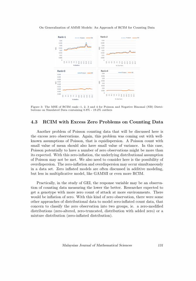
We now turn to discuss the influence of the percentages of outliers in thedata by setting increment of 0.8%, 1.7%, 2.5%, . . , 19.2% of outliers in the 15× 8 data matrix. Figure 3 shows that on a multiplicative model with lowestrank (rank = 1 and rank = 2) NB model of RCIM perform better than Poissonmodel, by smaller MSE. But in the more complex model, Poisson model givean exactly equal MSE to NB model. Here we can say that Poisson model canhandle the overdispersion by involving more interaction terms in its model.The more complex the model, the more severe overdispersed can be handled.



Figure 3: The MSE of RCIM rank=1, 2, 3 and 4 for Poisson and Negative Binomal (NB) Distri-butions on Simulated Data containing 0.8% - 19.2% outliers

4.3 RCIM with Excess Zero Problems on Counting Data

Another problem of Poisson counting data that will be discussed here isthe excess zero observations. Again, this problem was coming out with well-known assumptions of Poisson, that is equidispersion. A Poisson count withsmall value of mean should also have small value of variance. In this case,Poisson potentially to have a number of zero observations might be more thanits expected. With this zero-inflation, the underlying distributional assumptionof Poisson may not be met. We also need to consider here is the possibility ofoverdispersion. The zero-inflation and overdispersion may occur simultaneouslyin a data set. Zero inflated models are often discussed in additive modeling,but less in multiplicative model, like GAMMI or even more RCIM.

Practically, in the study of GEI, the response variable may be an observa-tion of counting data measuring the lower the better. Researcher expected toget a genotype with more zero count of attack at more environments. Therewould be inflation of zero. With this kind of zero observation, there were someother approaches of distributional data to model zero-inflated count data, thatconcern to classify the zero observation into two groups, ie. a zero-modifieddistributions (zero-altered, zero-truncated, distribution with added zero) or amixture distribution (zero-inflated distribution).



In this mixture distribution of zero-inflated, the zero will be classified intotwo groups, a group of positive (discrete) count distribution (Poisson or NB)occur with probability of 1−ω; the other represent the ’extra’ zero, occur withprobability of ω.

4.3.1 Zero-inflated Poisson in the RR-VGLM

ZIP model is powerful in dealing with counting data with excess zeros thanthe usual Poisson distribution, partly it is because the ZIP model also handlesoverdispersion. To see that, we will write down the probability mass function(p.m.f.) of the ZIP in two stages with two-components mixture distribution.

f(Y |θ, ω) =

{(1−ω)e−θθy

y! , for y = 1, 2, 3, ...

ω + (1− ω)e−θ, for y = 0;with 0 ≤ ω < 1(16)

Hadi and Sa’diyah (2014) write down the expectation of the p. m. f. to getthe mean and variance of ZIP as E(Y ) = µ and var(Y ) = µ+ (ω/(1− ω))µ2.For positive ω, the conditional distribution shows an overdipersion and the ZIPwill turn to a standard Poisson if ω = 0. The log-likelihood function of a vectorof random sample ZIP distributed as l(θ, ω;y), please see Hadi and Sa’diyah(2014) for more detail and also to get the joint model for ω and θ as

log ( ω1−ω ) = Gγ and

log (θ) = XB(17)

And in the linear predictors of RCIM model as (12) we now write η1 and η2 as

η =

(η1η2

)=

(logit ωlog µ

)(18)

There are two processes of how the data occurs, the first data is zero and thesecond is Poisson count data. Both processes are modeled respectively by η1and η2.

Which in the fact now, can be seen simply that this is a dimension reductionregression models ZIP or reduced-rank zero-inflated Poisson model (RR-ZIP).RR-ZIP is given by

logit ω = η1 = β(1)1 + α(1)1.η2 (19)

log µ = η2 = βT2 X (20)

with β(1)1 and α(1)1 are coefficients who want predictable.



With (19) and (20) the RR-ZIP model of rank=1 has H1 = I2 and H2 =

. . . = Hp =(α(1)1

)T . There is a trivial complication that the constraint angle(can use other constraints) imposed on parameters that are used instead of thefirst two. This can be simplified if the order parameter exchanged.

4.3.2 An Application of ZIP of RCIM for analysis of the GEI

Table 6 is the dataset of Hadi and Sa’diyah (2014). In this table we focusedon the endurance to leaf rust disease. The cells is the number of crops attackedby leaf-rust observed in three replications. A genotype with large numbers in-dicate the most vulnerability, and in vice verse, the smaller number the betterendurance. The zeros on the observation in Probolinggo sometimes called es-cape observation, where all the columns on this row are zero. The ZIP modelrelies on the assumption that zero are as structural and random ones. The ZIPmodel will provide us the probability of the cell to be zero, and the fitted valuefor Poisson count, as well.

Table 6: The 2nd data set: Count of Leaf Rust Disease Attacks on Mung Bean

Genotype EnvironmentsProboliggo Jember Jombang Bolo Rasanae

MLG1002 0 167 100 150 150MLG1004 0 217 250 233 250MLG1021 0 200 217 183 217MMC74dkp1 0 133 200 183 133MMC71dkp2 0 200 200 233 367MMC157dkp1 0 133 150 167 150MMC203dkp5 0 50 100 67 83MMC205e 0 50 67 100 67MMC100fkp1 0 50 83 83 83MMC87dkp5 0 83 117 133 83MURAI 0 0 50 33 33PERKUTUT 0 67 133 117 117

The data were analyzed using RCIM model, following Turner and Firth(2015) work on the Poisson distribution with the GAMMI model of Van Eeuwijk(1995). Determining the rank=2 model, here we use the deviance analysisrather than the log-likelihood ratio test as previously used in Hadi and Sa’diyah(2014).



Since Table 7 showed that the rank = 3 of ZIP model of RCIM does not fitthe data properly (p-value is greater than 0.05), then Table 8 determine thatZIP model of rank = 2 is the best way to explain the structure of the maineffects of additive and multiplicative interaction. With this rank = 2 of RCIM-ZIP model, the biplot is presented in Figure 4. It was done by run an RCIMmodel with rank = 0 and SVD-reparameterization on the working residuals toget the interaction visualization with rank = 2. The biplot variability is shownby the eigenvalues of matrix interaction. The first two eigenvalues, explain thetotal variability of the Biplot, that is 72.78%. The reader is recommended tosee Hadi and Sa’diyah (2014) in order to get more interpretation informationabout the GEI analysis of the biplot of Figure 4.

Table 7: The Deviance Analysis to test rank = 3 ZIP model of RCIM

Source df Deviance Mean Ratio of Mean p-valueDeviance DevianceMain Effects (Rank =0) 14 198.8616 14.2044 29.49009463 2.5013E-05RCIM Rank = 1 14 64.9406 4.6386 9.63033808 0.001572204RCIM Rank = 2 12 19.7904 1.6492 3.42394357 0.044636088RCIM Rank = 3 10 0.3172 0.0317 0.06585450 0.999882848Error 8 3.8533 0.4817Total 58 287.7631

Table 8: The Deviance Analysis to test rank = 2 ZIP model of RCIM

Source df Deviance Mean Ratio of Mean p-valueDeviance DevianceMain Effects (Rank =0) 14 198.8616 14.2044 61.30610867 2.9137E-12RCIM Rank = 1 14 64.9406 4.6386 20.02023257 3.80108E-08RCIM Rank = 2 12 19.7904 1.6492 7.11793771 0.000125675Error 18 4.1705 0.2317Total 58 287.7631



Figure 4: Biplot of the interaction effect on Log-scale of Zero-inflaated Poisson

4.3.3 Comparing a ZIP to a Poisson model in RCIM

Comparing ZIP model with Poisson model was done by Hadi (2012) usingdataset with zero-inflated of Table 6. Hadi (2012) said that Poisson modelfaced difficulties of computing in the estimation model of rank = 3. Thisfailure is expected to occur due to the failure of eigenvalue calculation becausethere is an infinite calculation. Meanwhile, at a lower rank, the log-likelihoodof ZIP model indicates that it is better than Poisson model. Obtaining thebest model depends on two things. The first is the link-functions concerningthe distribution of data and interpretation of the model, and the second is thedecomposition of the interaction, in this case, it is determined by the rankused. The higher the rank used, the more complex model we’ll get. In themore complex model, together with the distribution and its canonical link-function, the estimation parameters will paid a longer iteration of computing.Both of these works are inter-related and unseparable, especially when there isoverdispersion and/or excess zero. The best fit model can be obtained by theuse of distribution and proper link-function, and at the same time, also by thedegree of decomposition of the interaction (rank models).



Now we will use the 1st dataset of Table 1 that is modeled by a Poissonmodel to be compared with the ZIP model for count data with no zero problems.The RCIM ZIP able to model the structure of interaction on Poisson countingdata even though it contains no zero observation at all. This capability isindicated by ZIP model, since it has very similar results to Poisson models.Table 9 shows that log-likelihood value of the ZIP model is exactly the sameas Poisson model for a counting data with no zero.

Table 9: The Log-likelihood of ZIP and Poisson model of RCIM for data count with no zero

Model The ZIP Standard PoissonRCIM FullRank=3 -39.04556 -39.04556RCIM Rank=2 -39.09895 -39.09895RCIM Rank=1 -40.99432 -40.99432Main Effects(Rank=0) -48.33612 -48.33612

4.3.4 RCIM with Zero Inflated Negative Binomial Distributions

In this section, we will propose the ZINB for both overdispersion and/orexcess zero. Zero inflated Negative Binomial (ZINB) is one of the methods usedto deal with problem of overdispersion in a case of excess zero. ZINB formedby Negative Binomial distribution, mixture of the Poisson-Gamma and excesszero. A Negative Binomial distribution has parameters µ and α, the p. m. f.of random variable Y NB distributed can be written as:

fNB(y;µ, α) =Γ(yi + 1

α

)yi! Γ

(1α

) ( 1α

1α + µi

) 1α(

µi1α + µi

)yi(21)

A random variable Y of ZINB distribution has a valued of zero with probabilityof ω and follows the NB distribution with probability of (1 − ω). For Y = 0occur with probability of ω, then Y has p. m. f. of the form:



fZINB(y = 0;µ, α, ω) = ω + (1− ω)fNB(y = 0;µ, α)

= ω + (1− ω)Γ(0 + 1

α

)0! Γ

(1α

) ( 1α

1α + µ

) 1α(

µ1α + µ

)0

= ω + (1− ω)Γ(1α

)Γ(1α

) ( 1α

1α + µ

) 1α

= ω + (1− ω)

( 1α

1α + µ

) 1α

The rest occur with probability of (1− ω), Y = 1, 2, . . . , along with NB distri-bution:

fZINB(y 6= 0;µ, α, ω) = (1− ω) fNB(y 6= 0;µ, α)

= (1− ω)Γ(y + 1

α

)y! Γ

(1α

) ( 1α

1α + µ

) 1α(

µ1α + µ

)y

And the mixture distribution of ZINB means for ω = 0, the mean andvariance of ZINB will be equal to mean and variance of NB:

E(Y ) = (1− ω)µ

E(Y ) = (1− 0)µ

E(Y ) = µ

V ar(Y ) = E(Y )(1 + αµ+ ωµ)

V ar(Y ) = (1− 0)µ(1 + αµ+ ωµ)

V ar(Y ) = µ(1 + αµ)

As described in previous section, we will apply the linear predictors of RR-VGLM directly to those three parameters of ZINB distribution. We then com-pare the MSE of the ZINB versus the NB. Table 10 represents the MSE of thetwo methods (ZINB vs NB) on an overdispersed count data with zero’s prob-lems as we get from our simulation scenario. It shows that the MSE of ZINB



model is better than NB. It is concluded that RCIM ZINB fits excess zerosdata better than NB. Now we will move forward to discuss ZINB performancewith respect to the presence of outliers and excess zeros at once on the countingdata.

Table 11 contains the MSE of NB and ZINB model for data with severeillnesses conditions, which is (i) overdispersed counting data due to outliersand (ii) having zero problems, simultaneously. It seems that the MSE of ZINBmodel always smaller than NB’s at any ranks. This shows that ZINB modelfits the data (overdispersed with extra zeros) better than the NB model. Lastbut not least, we also evaluated the performance of ZINB model to count datacontaining structural zero of Table 6. Table 12, which represents the MSE ofNB and ZINB on counting data with structural zero, shows that although theZINB can provide smaller MSE than the NB’s at low rank of RCIM (rank = 1and 2), but at higher rank (rank = 3), NB performs better than ZINB one.

Table 10: The MSE of Negative Binomial (NB) and ZINB on overdispersed data with zero

Model MSE NB MSE ZINBRCIM rank = 1 0.20876010 0.07589846RCIM rank = 2 0.09743042 0.07504630RCIM rank = 3 0.10276670 0.02441078RCIM rank = 4 0.05146207 0.01666468RCIM rank = 5 0.02056970 0.00899084RCIM rank = 6 0.02681639 0.00535431

Table 11: The MSE of Negative Binomial and ZINB model on data with both outliers and extraszero (3rd scenario)

Model MSE NB MSE ZINBRCIM rank = 1 0.25555470 0.08142671RCIM rank = 2 0.14247590 0.07504630RCIM rank = 3 0.07846524 0.05165929RCIM rank = 4 0.05101145 0.05012614RCIM rank = 5 0.02153536 0.00899084RCIM rank = 6 0.01880404 0.00535431

Table 12: The MSE of Negative Binomial and ZINB model on count data with structural zero

Model MSE NB MSE ZINBRCIM rank = 1 0.02549026 0.02143623RCIM rank = 2 0.01268638 0.01260851RCIM rank = 3 9.86e-06 0.01209246



Table 13: The MSE of Negative Binomial and ZINB model on data with structural zero and alsooutliers at once (4th scenario)

Model MSE NB MSE ZINBRCIM rank = 1 0.02187914 0.03839160RCIM rank = 2 0.02145327 0.05245484RCIM rank = 3 1.06e-05 0.01474227

Table 13 presents the MSE of ZINB models for data containing both struc-tural zero and outliers at once. It seems that it is similar to Table 12, thatZINB better than NB at the lower rank model of RCIM, but less at higher. It’sclear that ZINB can be relied upon to model the data with structural zero withthe simplest interaction terms of RCIM. If we take a look at both Table 12 and13 across rows at the same column, we can see that when outliers come to datawith structural zeros, the MSE of both NB and ZINB will increase slightly.

5. Concluding Remark

Here we conclude that in multiplicative modeling, the overdispersion prob-lems of counting data can be handled in two ways. First by choosing the canon-ical link function of the distributional data. With the same rank of complexitythe NB can do better than usual Poisson.

The second, we make model the overdispersion by involving some moremultiplicative terms in our model. The standard Poisson model can fit theoverdispersed data properly with more complex multiplicative model than theNB one.

The ZIP model may overcome the problem of zero inflated, including thecounting data with structural zero. The ZIP give us the same result as Poissonfor the data with no zero. We proposed the ZINB model for overdispersedcounting data with excess zero, structural zero or containing outliers. TheZINB model result better fitted value for those counting data problems, by thesmaller MSE in multiplicative modeling.

Acknowledgement

We thank to Dimas, Graduated School of Mathematics, The University ofJember for LATEX helping. We also thank to Arif Musaddad, ILETRI, Malangfor early communication to get this joint paper writing partnership and thanks



to Thomas W. Yee, Department of Statistics, University of Auckland for theVGAM package and special thanks for his kindness during Hadi’s previousvisiting research.

References

Goodman, L. A. (1981). Association models and canonical correlation in theanalysis of cross-classifications having ordered categories. Journal of theAmerican Statistical Association, 76:320–334.

Hadi, A. F. (2012). The Developing of Robustness on Additive Main Effect -Multiplicative Interaction Models (AMMI). PhD thesis, Bogor AgriculturalUniversity, Bogor, Indonesia.

Hadi, A. F., Mattjik, A. A., and Sumertajaya, I. M. (2010). Generalized ammimodels for assessing the endurance of soybean to leaf pest. Jurnal IlmuDasar, 11:123–131.

Hadi, A. F. and Sa’diyah, H. (2014). Row-column interaction models for zero-inflated poisson count data in agricultural trial. Proc. ICCS-13, Bogor, In-donesia, 27:233 – 244. www.isoss.net/downloads/Prociccs13.pdf.

Hadi, A. F. and Sa’diyah, H. (2016). An approach of row-column interactionmodels (rcim) for generalized ammi models with deviance analysis. Agricul-ture and Agricultural Science Procedia, 9:134–145. http://dx.doi.org/10.1016/j.aaspro.2016.02.108.

Hilbe, J. M. (2011). Negative Binomial Regression Second Edition. CambridgeUniversity Press, New York, NY.

Pawitan, Y. (2001). In All Likelihood: Statistical Modelling and Inference UsingLikelihood. Oxford, Ireland : Clarendon Press.

Turner, H. and Firth, D. (2015). Generalized nonlinear models in R: Anoverview of the gnm package. R package version 1.0-8. http://CRAN.R-project.org/package=gnm.

Van Eeuwijk, F. (1995). Multiplicative interaction in generalized linear models.Biometrics, 51:1017–1032.

Yee, T. W. (2008). VGAM Family Functions for Positive, Zero-altered andZero-Inflated Discrete Distributions. University of Auckland, New Zealand,NZ. http://www.stat.auckland.ac.nz/.


www.isoss.net/downloads/Prociccs13.pdf

http://dx.doi.org/10.1016/j.aaspro.2016.02.108

http://dx.doi.org/10.1016/j.aaspro.2016.02.108

http://CRAN.R-project.org/package=gnm

http://CRAN.R-project.org/package=gnm

http://www.stat.auckland.ac.nz/


Yee, T. W. (2010). The vgam package for categorical data analysis. Journal ofStatistical Software, 32:1–34. http://www.jstatsoft.org/v32/i10.

Yee, T. W. (2014). Reduce-rank vector generalized linear models with twolinear predictors. Comput Stat Data Anal, 71:889 – 902.

Yee, T. W. (2015). Vector Generalized Linear and Additive Models: With anImplementation in R. Springer, New York, USA.

Yee, T. W. and Hadi, A. F. (2014). Row column interaction models, with anr implemetation. Computational Statistics, 29:1427–1445. http://dx.doi.org/10.1007/s00180-014-0499-9.

Yee, T. W. and Hastie, T. J. (2003). Reduced-rank vector generalized linearmodels. Statistical Modelling, 3:15–41.


http://www.jstatsoft.org/v32/i10

http://dx.doi.org/10.1007/s00180-014-0499-9

http://dx.doi.org/10.1007/s00180-014-0499-9

ongeneralizationofadditivemaineﬀectand ...einspem.upm.edu.my/journal/fullpaper/vol11sfeb/8. alfian...

Documents