one-way spillovers, endogenous innovator/imitator roles, and

Games and Economic Behavior 31, 1–25 (2000)doi:10.1006/game.1999.0734, available online at http://www.idealibrary.com on

One-Way Spillovers, Endogenous Innovator/ImitatorRoles, and Research Joint Ventures*

Rabah Amir

Department of Economics, Odense University, DK 5230 Odense M, DenmarkE-mail: [email protected]

and

John Wooders

Department of Economics, University of Arizona, Tucson, Arizona 85721E-mail: [email protected]

Received March 3, 1998

We consider a two-period duopoly characterized by a one-way spillover structurein process R&D and a very broad specification of product market competition. Weshow that a priori identical firms always engage in different levels of R&D, at equi-librium, thus giving rise to an innovator/imitator configuration and ending up withdifferent sizes. We also provide a general analysis of the social benefits of, and firms’incentive for, forming research joint ventures. Another contribution is methodolog-ical, illustrating how submodularity (R&D decisions are strategic substitutes) canbe exploited to provide a general analysis of a R&D game. Journal of EconomicLiterature Classification Numbers: C72, L13, O31. © 2000 Academic Press

Key Words: oligopolistic R&D; one-way spillovers; research joint ventures; sub-modularity.

1. INTRODUCTION

This paper develops a two-stage strategic model of process R&D/productmarket competition for an ex-ante symmetric duopoly under imperfect ap-propriability of R&D. In the model, at the first stage firms conduct pro-

*The authors thank Claude d’Aspremont, Kai-Uwe Kuhn, Stanley Reynolds, Lars-HendrikRoller, Bernard Sinclair-Desgagne, Peter Zemsky, and two anonymous referees, as well asseminar participants at C.O.R.E., INSEAD, the University of Arizona, the Free and HumboldtUniversities, Berlin, the W.Z.B./C.E.P.R. Conference on Industrial Policy, and the 1st Confer-ence on Industrial Organization at Carlos III—Madrid, for their comments and suggestions.

10899-8256/00 $35.00

Copyright © 2000 by Academic PressAll rights of reproduction in any form reserved.

2 amir and wooders

cess R&D and at the second stage, upon observing the final unit costs,firms compete in the product market. R&D is imperfectly appropriable,with R&D spillovers flowing from the firm with higher R&D activity toits rival (but never vice-versa) in a binomial fashion: With probability βa full spillover occurs and with probability �1 − β� no spillover occurs. Auni-directional spillover structure, such as this one, is appropriate when-ever there is a natural (complete) order to the cost-reducing innovationsthat can be achieved. In that case know-how may flow only from the firmfurther along in its R&D program to its less advanced rival.1

We derive two different sets of results. First, with a relatively wide scopeof generality in the product market specification, we establish the existenceof a subgame-perfect equilibrium, as well as a general characterization ofits properties. In particular, we show that no equilibrium can be symmetriceven though the two competing firms are ex ante identical. Thus an industryconfiguration endogenously emerges yielding an R&D innovator (the moreR&D intensive firm) and an R&D imitator. Firms differ in size (which ina Cournot or Bertrand framework is tied to unit production cost) and inR&D intensity (which might involve R&D strategy, lab type and size, andthe composition of R&D, were the R&D process explicitly modeled).

The second set of results concerns the performance comparison of acartelized research joint venture (RJV) or joint lab (denoted Case J) andpure R&D competition (denoted Case N). In Case J, R&D is conducted ina jointly owned lab run at equal cost by the firms together, whereas in CaseN each firm independently conducts R&D in its own lab. In both Case Jand Case N firms behave noncooperatively in the product market. The per-formance criteria of interest are R&D propensity, consumer surplus, andproducer surplus. Our main results here provide general conditions on theR&D cost function and the equilibrium second stage profit function whichinsure the superiority of the joint lab over R&D competition. These con-ditions boil down to demand being high enough relative to initial unit costand/or R&D costs being convex enough, depending on the criterion of in-terest. A version of the latter condition, which d’Aspremont and Jacquemin(1988) refer to as a second-order condition, is found in every paper in theR&D literature.

The present paper also makes a methodological contribution to the anal-ysis of two-stage games, in the context of a two-stage R&D game. Theapproach we introduce consists of representing the product market compe-tition at the second stage by a function 5�·; ·�, which gives the Nash profitto a firm as a function of the two post-R&D unit costs. An assumption

1In addition to its interpretation as the probability that a spillover occurs, the spilloverparameter β can also be interpreted in novel ways as an inverse measure of patent length, orof imitation lag: See Amir and Wooders (1999) for details.

r&d competition with one-way spillovers 3

fundamental to our analysis is that 5 is submodular. This assumption, aswell as the other basic assumptions of our analysis, are satisfied under thecommon specifications of Cournot competition, with either differentiatedor homogenous products, and Bertrand competition with sufficiently differ-entiated products. Therefore our analysis provides a unified treatment ofstrategic R&D encompassing most specifications of product market compe-tition considered in previous related work. Throughout the present paperan ancillary objective is to employ only minimally sufficient assumptions on5 needed for our results, thereby preserving as high a level of generalityas possible.

The submodularity of 5 is inherited by the overall payoff function ofthe two-stage game (thus making R&D decisions strategic substitutes, anatural property).2 This allows us to apply recent powerful results from thetheory of supermodular3 games in order to establish the existence of a purestrategy subgame-perfect equilibrium, to conduct the relevant comparativestatics analysis, and to obtain general answers in the evaluation of R&Dcooperation and competition. Standard existence results are not applicablesince the one-way nature of spillovers leads to the two-stage payoff havinga fundamental nonconcavity, independently of any curvature assumptionsplaced on the primitives of the model.

Our results relate to two different strands of literature, one on intra-industry heterogeneity and the other on R&D cooperation. In the litera-ture on intra-industry heterogeneity Katz and Shapiro (1987) and Boyerand Moreaux (1997) also deal with R&D models, while Hermalin (1994)considers firms’ internal control structures. These paper all develop ex-ante symmetric models with only asymmetric equilibria.4 Related studiesin evolutionary economics and management strategy have been around fora longer time: see Roller and Sinclair-Desgagne (1996) for a survey.

R&D cooperation has already been investigated by Katz (1986), d’Aspre-mont and Jacquemin (1988, 1990) (henceforth referred to as AJ) andKamien et al. (1992) (henceforth KMZ). In these papers spillovers aremulti-directional, the spillover parameter measuring the fraction of afirm’s R&D activity that spills to each of its rivals (see Amir (1998) for acomparative critique). With linear demand and a general R&D cost func-tion, KMZ establishes that Case J dominates Case N (as well as each of

2See Athey and Schmutzler (1995) for complementarities in R&D types in a one-firmmodel, and Bagwell and Staiger (1994) for a setting more related to ours.

3See Topkis (1978, 1979, 1998), Vives (1990), Milgrom and Roberts (1990a), Milgrom andShannon (1994), and Amir (1996b).

4This contrasts with the literature on industry dynamics where exogenous idiosyncraticshocks lead to a heterogeneous distribution of characteristics among perfectly competitivefirms: see Jovanovic (1982), Lambson (1992), Hopenhayn (1992), and Flaherty (1980).

4 amir and wooders

the other R&D scenarios they consider) for the performance criteria ofinterest.

The analysis of AJ, based on linear demand and a quadratic R&D costfunction, has inspired numerous follow-up papers investigating various as-pects of R&D cooperation.5 Within the same specification as AJ, but withone-way spillovers, Amir and Wooders (1999) provide a complete charac-terization that nicely complements the present analysis.

The paper is organized as follows: in Section 2 we introduce our modelof R&D competition with one-way spillovers and analyze its equilibria. InSection 3 we compare R&D competition and RJV cartelization. Proofsof our results, as well as a brief summary of some (simplified) results onsubmodular games needed here, are provided in the Appendix.

2. THE NONCOOPERATIVE MODEL

2.1. The Model

Consider an industry composed of two a priori identical firms, each withinitial unit cost c, engaged in a two-stage game. In the first stage, Firms 1and 2 decide on unit cost reduction x and y, with x; y ∈ �0; c�, on the basisof a known R&D cost schedule f �·�. In the second stage, upon observingthe new unit costs, the firms compete in the product market by choosingoutputs (i.e., Cournot competition) or prices (i.e., Bertrand competition).There is no need to specify the mode of competition as the equilibriumprofits of the second stage are modeled by a general function which hasboth models as special cases.

While this two-stage framework is standard in the recent R&D literature,our set-up departs from previous ones in the way imperfect appropriabil-ity of R&D is modelled. We consider R&D processes where leakages flowonly from the more R&D-active firm to the rival in an all-or-nothing prob-abilistic fashion. Specifically, given autonomous cost reductions by Firms 1and 2 of x and y, respectively, with (say) x ≥ y, the effective (or final) costreductions are given by X and Y , respectively, with

X = x and Y ={x with probability βy with probability 1− β: (2.1)

This spillover process is a natural one in a number of different contexts.6

If there is a complete order to the cost-reducing innovations that can be

5See Henriques (1990), DeBondt et al. (1992), and Suzumura (1992), among numerousothers. See also Amir and Wooders (1998).

6Another reasonable spillover process is the deterministic analog, defined by X = x andY = y + β�x − y� = βx + �1 − β�y: Unfortunately, payoffs in the two-stage game are notsubmodular for large β under this process, as the reader can easily verify.


undertaken, then only the more R&D-active firm can generate spillovers.Alternatively, if there are many different R&D programs that a firm canundertake, but R&D programs are unrelated, then β can be interpreted asthe probability that the less R&D active of the two firms is successful inimitating its rival.7 See Amir and Wooders (1999) for a detailed discussionof these and other interpretations.

We restrict attention to subgame-perfect equilibria. A (pure) strategyfor Firm i is a pair �xi; ai� where xi ∈ �0; c� is firm i’s autonomous costreduction and ai: �0; c�2 → � is a map from profiles of post-R&D unitcosts to the set of product market decisions (outputs or prices). The overallpayoff to a firm is simply its second-stage profit minus its first-stage R&Dcost.

The following basic assumptions are in effect throughout the paper.

(A1) For every pair of R&D decisions �x; y� ∈ �0; c�2, the second-stage (product market) game has a unique Nash equilibrium, with corre-sponding payoffs (i.e., profits) given by a function 5 of the two firms’ postR&D unit costs. Here, 5�·; ·� denotes the Nash profits of the firm whoseunit cost is the first argument.

(A2) (i) 5: �0; c�2 → � is continuous, and strictly submodular.

(ii) 5 is nonincreasing (nondecreasing) in its first (second) argu-ment.

(iii) 5�c1; c1� < 5�c2; c2� if c1 > c2:

(A3) f is nondecreasing and f �0� ≥ 0.

Some of our results require the following smoothness assumption (withPart (ii) of (A4) being a minor strengthening of (A2)(iii) given (A2)(ii)).8

(A4) (i) 5 and f are twice continuously differentiable.

(ii) �51�z; z�� > �52�z; z��, for all z ∈ �0; c�.A major innovation in the present paper is our treatment of the product

market competition, which we now argue offers a broad scope of gener-ality in at least two different situations. The first situation is the standardone, whereby the second stage represents a one-shot game in product mar-ket decisions. In this context, Assumptions (A1)–(A4) may be justified andinterpreted as follows. The equilibrium uniqueness assumption (A1) is con-venient, if somewhat restrictive. For the Cournot model, for instance, Amir

7When R&D programs are inter-related, each firm can benefit from the R&D activity ofits rival, and one of the standard multi-way deterministic spillover processes would be moreadequate (see AJ and KMZ).

8Indeed, as (A2)(iii) says that 5�z; z� is decreasing in z, we have (with smoothness) that51�z; z� +52�z; z� ≤ 0; which is nearly the same as (A4)(ii).

6 amir and wooders

(1996b) shows that it holds whenever P�·� − ci is a log-concave function,where P�·� is the inverse demand function and ci is the unit cost of Firm i,i = 1; 2. This is implied, in particular, by P�·� itself being log-concave, andis thus more general than most studies using the Cournot model. For theBertrand model with differentiated products, Milgrom and Roberts (1990a)give a uniqueness argument for a variety of commonly used specifications.

(A2)(i) may be viewed as a (negative) complementarity condition as itholds that the improvement in a firm’s profit resulting from a drop in owncosts increases with the cost of the rival firm. (A2)(ii) is self-explanatory:a firm’s profit decreases with own cost, but increases with rival’s cost.(A2)(iii) says that in a symmetric duopoly, a unit drop in both firms’ costsraises their profits. Put differently, own cost effects dominate rival’s cost ef-fects on profit. While reasonable, this assumption does impose restrictionson demand in a Cournot setting: see Seade (1985) or Kimmel (1992) for adetailed treatment of this issue. Finally, (A3) is clearly a natural assump-tion.

We now discuss the generality of our approach. First, observe that As-sumptions (A1)–(A4) are all satisfied in the commonly adopted cases of

(i) Cournot competition with linear demand P�Q� = a − bQ andunit costs k1, k2, which leads to equilibrium profits given by 5�k1; k2� =�a− 2k1 + k2�2/9b, and

(ii) Bertrand competition with differentiated products, linear demandqi = a−pi + bpj , 0 < b < 1, i; j = 1; 2, i 6= j, and units costs k1; k2, whichleads to equilibrium profits equal to 5�k1; k2� = ��2 + b�a− �2 − b2�k1 +bk2�2.

Other examples which can easily be verified as satisfying (A1)–(A4) in-clude Cournot competition with a quadratic demand function P�Q� = a−bQ2, Q ≤ √a/b, which leads to equilibrium profits equal to 5�k1; k2� =1

16�2a+ k2 − 3k1�2/√b�2a− k1 − k2�; or Cournot competition with linear

demand and differentiated products. On the other hand, with hyperbolic de-mand P�Q� = �Q + 1�−1 it can be checked (see Mirman et al., 1994) that(A2)(i) fails to hold. Nonetheless, since most studies in the R&D literatureare based on linear demand, the present treatment constitutes a major im-provement in generality. Another desirable feature of this approach is itsunifying power; it dispenses with the usual distinctions between Cournotand Bertrand competition, and homogeneous and differentiated products,thus allowing a comprehensive treatment of the effects of process-R&D onmarket competition.

The second possible situation to which the two-stage model at hand canbe applied is a novel one made possible by our approach. Here, 5 mayrepresent the overall equilibrium payoff to a multi-stage game, possiblywith an infinite horizon, and in several product markets simultaneously.


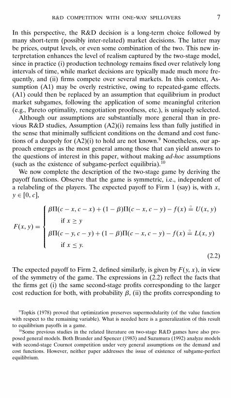
In this perspective, the R&D decision is a long-term choice followed bymany short-term (possibly inter-related) market decisions. The latter maybe prices, output levels, or even some combination of the two. This new in-terpretation enhances the level of realism captured by the two-stage model,since in practice (i) production technology remains fixed over relatively longintervals of time, while market decisions are typically made much more fre-quently, and (ii) firms compete over several markets. In this context, As-sumption (A1) may be overly restrictive, owing to repeated-game effects.(A1) could then be replaced by an assumption that equilibrium in productmarket subgames, following the application of some meaningful criterion(e.g., Pareto optimality, renegotiation proofness, etc.), is uniquely selected.

Although our assumptions are substantially more general than in pre-vious R&D studies, Assumption (A2)(i) remains less than fully justified inthe sense that minimally sufficient conditions on the demand and cost func-tions of a duopoly for (A2)(i) to hold are not known.9 Nonetheless, our ap-proach emerges as the most general among those that can yield answers tothe questions of interest in this paper, without making ad-hoc assumptions(such as the existence of subgame-perfect equilibria).10

We now complete the description of the two-stage game by deriving thepayoff functions. Observe that the game is symmetric, i.e., independent ofa relabeling of the players. The expected payoff to Firm 1 (say) is, with x;y ∈ �0; c�,

F�x; y� =

β5�c − x; c − x� + �1− β�5�c − x; c − y� − f �x� ◦= U�x; y�if x ≥ y

β5�c − y; c − y� + �1− β�5�c − x; c − y� − f �x� ◦= L�x; y�if x ≤ y:

(2.2)

The expected payoff to Firm 2, defined similarly, is given by F�y; x�, in viewof the symmetry of the game. The expressions in (2.2) reflect the facts thatthe firms get (i) the same second-stage profits corresponding to the largercost reduction for both, with probability β, (ii) the profits corresponding to

9Topkis (1978) proved that optimization preserves supermodularity (of the value functionwith respect to the remaining variable). What is needed here is a generalization of this resultto equilibrium payoffs in a game.

10Some previous studies in the related literature on two-stage R&D games have also pro-posed general models. Both Brander and Spencer (1983) and Suzumura (1992) analyze modelswith second-stage Cournot competition under very general assumptions on the demand andcost functions. However, neither paper addresses the issue of existence of subgame-perfectequilibrium.

8 amir and wooders

their autonomous cost reductions with probability �1− β�, and (iii) pay fortheir autonomous cost reduction only.

It is easy to see that F inherits the continuity property of 5 (from As-sumption (A2)(i)). It turns out that F also inherits the submodularity of 5(also in (A2)(i)), but not the differentiability of 5 and f , which fails alongthe diagonal of �0; c�2, or the concavity of each line in (2.2) assumed belowfor some of our results. This is intended only as a preview here and will beestablished later.

2.2. Properties of the Noncooperative R&D Model

Here, we state and interpret our results for the two-stage game underconsideration. Since the second-stage game admits a unique Nash equi-librium, every Nash equilibrium �x∗; y∗� of the game with payoffs (2.2) in-duces a subgame-perfect equilibrium of the two-stage game, and vice-versa.In view of this one-to-one correspondence, we use the two terminologiesinterchangeably.

We begin with the fundamental property of the game at hand (strategicsubstitutability), and a key structural characteristic of its equilibria (asym-metry).

Theorem 2.1. Assume (A1)–(A2) hold. Then the following are true:

(i) The game with payoffs (2.2) is submodular, and hence has a pure-strategy Nash equilibrium.

(ii) Every interior pure-strategy Nash equilibrium is asymmetric if (A4)holds and β > 0 .

(iii) Every pure-strategy Nash equilibrium is asymmetric if, in additionto the hypothesis of (ii), the following holds (here subscripts denote partialderivative) :

f ′�0� < −β52�c; c� −51�c; c� and f ′�c� > −�1− β�51�0; 0�: (2.3)

A discussion of these results is provided at the end of this subsection.The next result deals with uniqueness of equilibrium. Observe that in viewof the symmetry of the game and the fact that no equilibrium can involvethe firms taking the same decisions (Theorem 2.1), the sharpest uniquenessresult would yield two equilibria.

Theorem 2.2. Under Assumptions (A1)–(A4) and (2.3), the R&D game(with payoffs (2.2)) has exactly two pure-strategy Nash equilibria, of the form�x; x� and �x; x�, with (say) x > x, if in addition β ∈ �0; 1� and

f ′′�·� > (511 −512

)�c − �·�; z�; ∀z ∈ �0; c� (2.4)

and

f ′′�·� > (511 + 2512 +522

)�c − �·�; c − �·��: (2.5)


FIGURE 1

Define the best-response correspondence in the usual way, i.e., (say) forFirm 1, r1�y� = arg max�F�x; y�: x ∈ �0; c��. The next result holds thatr1 and r2 are essentially as depicted in Figure 1 (note that r1 = r2, bysymmetry).

Lemma 2.3. Under the hypothesis of Theorem 2.2 (i.e., (A1)–(A4), (2.3)–(2.5)), r1 and r2 are continuous nonincreasing functions everywhere in �0; c�except at one point d ∈ �0; c� where ri�d−� > d > ri�d+�.

The last results in this section deal with comparative statics of the equi-librium �x; x� as the probability of a spillover increases in �0; 1�.

Theorem 2.4. Under (A1) and (A2), the following hold as β increases in�0; 1�:

(i) Holding one firm’s R&D level constant, the extremal best-responsesof the other firm are nonincreasing (in other words, r1 and r2 shift down).

(ii) The total equilibrium R&D level x+ x (associated with the uniqueNash equilibrium pair �x; x� and �x; x�) decreases if, in addition, (2.4) and(2.5) hold.

10 amir and wooders

(iii) x itself decreases if, in addition, (2.4) and (2.5) and the followinghold:

f ′′�·� ≥ �1− β�[511�c − �·�; c − z�

+ 51�c − �·�; c − z�512�c − z; c − �·��51 +52��c − z; c − z� −51�c − z; c − �·��

];

∀z > �·�; ∀β: (2.6)

To gain insight into the nature of Conditions (2.3)–(2.6), it is instructiveto consider them under the well-known cases of (a) Cournot competitionwith linear demand and homogeneous goods, and (b) Bertrand competitionwith linear demand and differentiated goods, both with R&D cost functionf �x� = γ

2x2. Leaving out the computational details we note that (i) the first

part of (2.3) always holds for both (a) and (b), (ii) the second part of (2.3)becomes 9bγ > 4�1− β� a

cfor Case (a) and γ > 2�1− β��2 − b2��2 + b� a

cfor Case (b), (iii) (2.4) becomes 9bγ > 12 for Case (a) and γ > �b+ 2�2�1−b�2 for Case (b). Finally, a sufficient condition can be derived for (2.6):9γ > 16�1− β� for Case (a), which is shown in Amir and Wooders (1999)to be rather tight, and γ ≥ 4�1− β��2− b2�2 for Case (b). It is worthwhileto observe that all these seemingly different conditions boil down to somecommon qualitative requirements: that R&D costs be sufficiently convex,and/or market size be sufficiently small (relative to cost), and/or spilloversor extent of product homogeneity be sufficiently high. Conditions similarto γ being large enough have been used in all related work following AJ(who refer to them as second-order conditions).

We now provide a discussion of the results of this section. Theorem 2.1(i)suggests that our model is well defined under remarkably general condi-tions. In particular, the absence of any concavity assumptions on the payofffunction F is new in the R&D literature. For the overall payoff functionF to inherit the submodularity property of the equilibrium profit function5, Assumption (A2)(iii) is crucial. Submodularity of F here has the usualnegative complementarity interpretation: The marginal returns to increas-ing R&D expenditures decrease with the rival’s R&D expenditure, andthis holds independently of whether the firm is receiving or giving awayspillovers!

In view of the asymmetry of equilibria, our model is a natural candidatefor explaining the ubiquitous inter-firm heterogeneity within most indus-tries. The driving force behind this endogenous firm heterogeneity is theanticipation of (probabilistic) R&D spillovers from the leading firm to itsrival. Under such a spillover structure, firms endogenously emerge withdifferent production cost structures through the very process of adopting(costly) technological progress. Thus, the competing firms end up with dif-


ferent levels of R&D activity (hence with different types of R&D strat-egy/labs), different firm sizes, and different market shares in the productmarket.

Theorem 2.2 is a convenient result as it allows for more straightforwardanalysis of equilibrium behavior, unencumbered by the difficulties associ-ated with multiple equilibria. For instance, it is needed for clear-cut answersto the comparative statics analysis of Theorem 2.4. Both theorems requireassumptions on f ′′, which translate into strong convexity of f since 5 is typ-ically convex in own costs or even jointly. Similar assumptions have alwaysbeen made in related studies (e.g., AJ, KMZ), and are needed to insure thatpayoffs are concave in own R&D decision. In our model, such assumptionscan only yield concavity of each line in (2.2), but not of F itself.

While Theorems 2.4(i) and (ii) are intuitively clear, (iii) is perhaps lessso. The fact that each firm would decrease its R&D level as β increases,holding the rival’s R&D level constant, does not imply that, at equilibrium,both R&D levels go down.11 In other words, there are two effects governingthe response of x (say) to changes in β. The first is captured in 2.4(i) andis rather intuitive: The leading firm (or innovator) cuts down on R&D asthe likelihood of full spillover to the rival increases, with the rival’s R&Dlevel constant. However, if the rival also decreases his R&D level, the othereffect is that the firm under consideration will want to respond by increasingR&D activity. The overall effect on x then depends on the relative strengthof these two effects. Condition (2.6) is needed to shift the balance towardsa decline of x, i.e., towards the first effect. To see this, observe that thef ′′ on the LHS of (2.6) refers to the imitator’s cost function, the intuitionbeing that if the latter’s second derivative is large, x does not respond muchto changes in β and in x; so that the first effect above is the dominant one.

Finally, since the payoffs are continuous, the game at hand has a sym-metric mixed-strategy equilibrium in R&D decisions. Since the game is su-permodular, the support of the mixed strategies at equilibrium would be�x; x�. Under such a solution, the firms would still end up (endogenously)different with positive probability.

3. RESEARCH JOINT VENTURES

We consider here different R&D cooperation schemes among firmswhich remain competitors in the product market. These schemes are char-

11In the language of supermodularity analysis, one cannot find orders on the two actionssets that would make each payoff supermodular in the two decisions and in the pair (owndecision, β). Hence, the comparative statics result for supermodular games cannot be invoked(Milgrom and Roberts, 1990a; Sobel, 1988).

12 amir and wooders

acterized by two key features: whether firms coordinate in choosing R&Dexpenditure (i.e., “collude” in the first-stage of the game), and whetherfirms cooperate in the actual conduct of R&D (by increasing β).

Here, we are mainly concerned with only one RJV scenario: the jointlab. This is characterized by the firms running one joint R&D facility athalf the cost each, and will be denoted by J. We note below that J isequivalent (for our model) to KMZ’s case CJ, or cartelized RJV, wherebyfirms coordinate R&D expenditures in the first-stage and fully communicateduring the R&D process (i.e., set the spillover rate equal to 1).

In the course of investigating the properties of Case J, it turns out thatit is useful to also consider the following broader RJV specification. LetCs denote the scenario whereby firms coordinate their R&D investments(so as to maximize total profits), while the spillover parameter is givenby s ∈ �0; 1�. Thus, in particular, s = 0; β; 1 stand for the cases wherethe spillover rate is reduced to 0, kept as it is, and increased to 1 (itsmaximum value), respectively.12 Note that the case s < β is not necessarilyeconomically meaningful within the context of our model in the sense thatspillovers are generally thought of as being unpreventable by the firms.Nonetheless, the case s = 0 is particularly useful below for comparativepurposes.

The joint objective function of the two firms in Case Cs (assuming w.l.o.g.that x ≥ y) is to maximize F�x; y� + F�y; x� over x; y in �0; c�, with β setequal to s, which reduces to

2s5�c−x; c−x�+ �1− s�[5�c−x; c− y�+5�c− y; c−x�]− f �x�− f �y�:(3.1)

The single-firm objective in Case J is to maximize over x ∈ �0; c�5�c − x; c − x� − 1

2f �x�: (3.2)

Observe that (3.1) reflects the (potential) operation of two separate R&Dlabs by the cartel, with variable spillover parameter, while (3.2) reflects theoperation of one joint lab with equal cost sharing. In Case J a symmetricoutcome necessarily obtains. As will be seen below, this may or may notbe true for Case Cs, s ∈ �0; 1�. In both cases, the two firms compete in theproduct market, as captured by 5.

Our central concern in this section is a performance comparison be-tween the noncooperative model of Section 2 (to be denoted N) and CaseJ (which we show below to be essentially equivalent to Case C1). The per-formance criteria of interest here are: propensity for R&D, firm profits,

12The case Cβ here is clearly the analog of the second scenario analyzed in AJ. See Salantand Shaffer (1998) on the emergence of asymmetry in Case Cβ.


consumer and social welfare. The cases C0 and Cβ are analyzed here onlyas useful intermediate steps in the overall analysis.

We first point out that Cases J and C1 are interchangeable in the follow-ing sense.

Lemma 3.1. Cases J and C1 are equivalent in the sense that they both leadto the same optimal R&D levels and the same optimal total profits.

It is still convenient to have the two cases as Case J is more readilyinterpretable and has symmetry built into it, while Case C1 is useful belowthrough its properties as the limit case of Cs as s→ 1.

Our first comparison of Cases J and N concerns R&D propensities. Thisrequires, however, an intermediate lemma which is of independent interest,a comparison between Case J and Case N with β = 0 (the latter is denotedN0 below). In dealing with this comparison, an additional assumption is nowintroduced as a new version of (A4). It quantifies the dependence of profitson own versus cross cost reductions in a symmetric duopoly setting.

(A5) 5 and f are twice continuously differentiable and �51�z; z�� ≥2�52�z; z��; for all z ∈ �0; c�.

Clearly, (A5) is a stronger version of (A4). It is easily seen to be satis-fied under Cournot competition with linear demand, with strict inequalityif products are differentiated and with equality for homogeneous products.For Bertrand competition with differentiated products, (A5) can be seen tohold if and only if the cross-demand coefficient (denoted by b in the discus-sion of (A1)–(A3) in Section 2) is in the interval �0;√3 − 1� ≈ �0; :73�,13

i.e., as long as demand is somewhat away from the well-known case of ho-mogenous products (b = 1).14

Lemma 3.2. Under Assumptions (A1)–(A3), (A5) and (2.4), we have

(i) In Case N0, there is a unique and symmetric equilibrium �x0; x0�.(ii) The equilibrium R&D level of Case J, xJ , satisfies xJ ≥ x0.

We are now ready for the comparison of R&D propensities and profits(interpretations of the results are given later on).

13In their treatment of Bertrand competition, KMZ give 23 as a lower bound for this critical

value of b. Since our model and theirs are equivalent when β = 0 and demand is linear, thefact that our bound is sharper indicates that (A5) is tight (see also the proof of Lemma 3.2(ii)).

14It can easily be seen that the 5 function corresponding to the case b = 1, given by

5�c1; c2� ={ �c2 − c1�D�c2� if c1 < c2

0 if c1 ≥ c2;

(where D�·� is the demand function) is not submodular in �c1; c2�. Hence this case fails As-sumption (A2) anyway, and thus does not fit our model.

14 amir and wooders

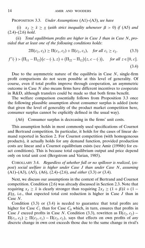
Proposition 3.3. Under Assumptions (A1)–(A3), we have

(i) xJ ≥ x ≥ x (with strict inequality whenever β > 0) if (A5) and(2.4)–(2.6) hold.

(ii) Total equilibrium profits are higher in Case J than in Case N , pro-vided that at least one of the following conditions holds:

25�c2; c2� ≥ 5�c1; c2� +5�c2; c1�; for all c1 ≥ c2: (3.3)

f ′′�·�> (511−512)(c−�·�; z)+ (522−512

)(z; c−�·�); for all z ∈ �0; c�:

(3.4)

Due to the asymmetric nature of the equilibria in Case N , single-firmprofit comparisons do not seem possible at this level of generality. Ofcourse, even if total profits improve through cooperation, an asymmetricoutcome in Case N also means firms have different incentives to cooperatein R&D, although transfers could be made so that both firms benefit.

The welfare comparison essentially follows from Proposition 3.3 oncethe following plausible assumption about consumer surplus is added (notethat given the level of generality of the product market competition here,consumer surplus cannot be explicitly defined in the usual way).

(A6) Consumer surplus is decreasing in the firms’ unit costs.

This assumption holds in most commonly used specifications of Cournotand Bertrand competition. In particular, it holds for the cases of linear de-mand reported in Section 2. For Cournot competition (with homogeneousproducts), it actually holds for any demand function, provided productioncosts are linear and a Cournot equilibrium exists (see Amir (1996b) for ex-act conditions). This is because total equilibrium output and price dependonly on total unit cost (Bergstrom and Varian, 1985).

Corollary 3.4. Regardless of whether full or no spillover is realized, (ex-post) social welfare is higher under Case J than under Case N , assuming(A1)–(A3), (A5), (A6), (2.4)–(2.6), and either (3.3) or (3.4).

Next, we discuss our assumptions in the context of Bertrand and Cournotcompetition. Condition (2.6) was already discussed in Section 2.3. Note thatrequiring xJ ≥ x is clearly stronger than requiring 2xJ ≥ �1 + β�x + �1 −β�x, i.e., that expected total cost reduction is higher in Case J than inCase N .

Condition (3.3) or (3.4) is needed to guarantee that total profits arehigher for Case C1 than for Case C0 which, in turn, ensures that profits inCase J exceed profits in Case N . Condition (3.3), rewritten as 5�c2; c2� −5�c1; c2� ≥ 5�c2; c1� − 5�c2; c2�; says that effects on own profits of anydiscrete change in own cost exceeds those due to the same change in rival’s


cost, starting from a symmetric duopoly. Thus (3.3) strengthens (A4)(ii)which says the same thing but only for infinitesimal changes. Under Cournotcompetition with linear demand condition (3.3) is equivalent to 2a+ 3c2 −5c1 ≥ 0 (with c2 ≤ c1). Since c2 ≥ 0 and c1 ≤ c, a sufficient condition for(3.3) in this case is 2a ≥ 5c. Thus (3.3) amounts to requiring demand to behigh (relative to costs).

Condition (3.4) is needed to ensure concavity of the joint objective inCase C0, therefore resulting in a symmetric R&D choice for this case.Hence (3.4) works by removing the asymmetry bias captured in Lemma 3.5(see below). When symmetry prevails in Case C0, the cartelized firms pre-fer full to no spillover. Under Cournot competition with linear demandCondition (3.4) is equivalent to 9γ > 18, and hence requires that the R&Dcost function be sufficiently convex. Both (3.3) and (3.4) have analogousinterpretations for Bertrand competition.

We now provide a discussion of the results of this section emphasiz-ing their relationship to related work on RJVs, namely, AJ and KMZ. Asdiscussed in the Introduction, one motivation of the present paper is a re-examination of the principal conclusion from related work: that a joint labor cartelized RJV dominates R&D competition in terms of equilibriumprices (and thus consumer welfare), firm profits, and hence social welfare.The reasons for questioning the validity of this conclusion in the presentcontext are (i) the lack of generality of the previous analyses, (ii) the newspillover process introduced, and (iii) the fact that Case J yields symmet-ric outcomes as a built-in feature while Case N always leads to asymmetricequilibria. This last feature is important since, in typical specifications ofCournot and Bertrand competition (see examples in Section 2.1), the 5function is jointly convex and thus firms (jointly) prefer not to compete onequal terms in the product market, as we now show.

Lemma 3.5. Let 5 be jointly convex on �0; c�2, k > 0 and consider thefollowing objective (with constraint):{

5�c1; c2� +5�c2; c1�: c1 + c2 = k}: (3.5)

Then the arg max of (3.5) consists of �0; k� and �k; 0�, while the arg min is�k2 ; k2 �.

Roughly, the main finding here is that, in the present context, the prin-cipal conclusion of the RJV literature crucially requires new assumptions,i.e., (2.6) and (3.3) or (3.4), to ensure its validity.

Finally, observe that for Case N0, our model is equivalent to AJ’s andKMZ’s. Thus, our Lemma 3.2(ii) may be viewed as a generalization oftheir analogous result to a broader class of profit functions (instead of thatcorresponding to linear demand).

16 amir and wooders

APPENDIX

Summary of Submodular Optimization/Games

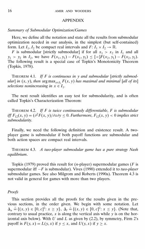
Here, we define all the notation and state all the results from submodularoptimization needed in our analysis, in the simplest (but self-contained)form. Let I1; I2 be compact real intervals and F : I1 × I2 → �.F is submodular [strictly submodular] if for all x1 > x2 in I1 and all

y1 > y2 in I2, we have F�x1; y1� − F�x1; y2� ≤ �<�F�x2; y1� − F�x2; y2�:The following result is a special case of Topkis’s Monotonicity Theorem(Topkis, 1978).

Theorem 4.1. If F is continuous in y and submodular [strictly submod-ular] in (x; y�, then arg maxy∈I2

F�x; y� has maximal and minimal [all of its]selections nonincreasing in x ∈ I1.

The next result identifies an easy test for submodularity, and is oftencalled Topkis’s Characterization Theorem:

Theorem 4.2. If F is twice continuously differentiable, F is submodulariff F12�x; y� = �∂2F�x; y�/∂x∂y ≤ 0. Furthermore, F12�x; y� < 0 implies strictsubmodularity.

Finally, we need the following definition and existence result. A two-player game is submodular if both payoff functions are submodular andboth action spaces are compact real intervals.

Theorem 4.3. A two-player submodular game has a pure strategy Nashequilibrium.

Topkis (1979) proved this result for (n-player) supermodular games (F issupermodular iff −F is submodular). Vives (1990) extended it to two-playersubmodular games. See also Milgrom and Roberts (1990a). Theorem 4.3 isnot valid in general for games with more than two players.

Proofs

This section provides all the proofs for the results given in the pre-vious sections, in the order given. We begin with some notation. Let1u

◦= ��x; y� ∈ �0; c�2: x ≥ y�; 1l ◦= ��x; y� ∈ �0; c�2: x ≤ y�. (Note that,contrary to usual practice, x is along the vertical axis while y is on the hor-izontal axis below). With U and L as given by (2.2), by symmetry, Firm 2’spayoff is F�y; x� = L�y; x� if y ≤ x, and U�y; x� if y ≥ x.


FIGURE 2

Proof of Theorem 2.1. (i) We show that F , as given by (2.2), is strictlysubmodular in �x; y�.15 To this end, fix x1; x2; y1; y2 in �0; c� with x1 >x2; y1 > y2. If all four points �x1; y1�; �x1; y2�; �x2; y1�; and �x2; y2� liein 1u or in 1l, strict submodularity of F follows directly from the strictsubmodularity of 5 (i.e., Assumption (A2)(i)), since only the middle termof U and L depends on both x and y.

If some of the four points lie in 1u and the rest in 1l, it is easily seenthat there are four different cases. It turns out that the proofs of strictsubmodularity of F are all similar, so we present the case depicted in Fig. 2;i.e., �x1; y1�; �x1; y2�; �x2; y2� are in 1u while �x2; y1� is in 1l. We must thenshow that U�x1; y1� − U�x1; y2� < L�x2; y1� − U�x2; y2�. We clearly have,given the location of the points, x2 < y1. Hence, by Assumption (A.2)(iii),

0 ≤ β5�c − y1; c − y1� − β5�c − x2; c − x2�: (4.1)

15Note that Topkis’s Characterization Theorem cannot be used here, since F is not differ-entiable along the diagonal in �0; c�2, but it can be used in the interior of 1u and 1l separately.On the other hand, Theorem 2* of Milgrom and Roberts (1990b) is an alternative approachto this proof.

18 amir and wooders

Since 5 is strictly submodular and f only depends on one variable,[�1− β�5�c − x1; c − y1� − f �x1�]− [�1− β�5�c − x1; c − y2� − f �x1�

]≤ [�1− β�5�c − x2; c − y1� − f �x2�

]− [�1− β�5�c − x2; c − y2� − f �x2�

]: (4.2)

Adding up (4.1), (4.2) and the trivial equality β5�c − x1; c − x1� −β5�c −x1; c − x1� = 0 and rearranging terms yields[

β5�c − x1; c − x1� + �1− β�5�c − x1; c − y1� − f �x1�]

− [β5�c − x1; c − x1� + �1− β�5�c − x1; c − y2� − f �x1�]

<[β5�c − y1; c − y1� + �1− β�5�c − x2; c − y1� − f �x2�

]− [β5�c − x2; c − x2� + �1− β�5�c − x2; c − y2� − f �x2�

];

which says that F is strictly submodular for the four-point choice of Fig. 2.This last inequality is strict since (4.1) is strict if β > 0 and (4.2) is strict ifβ < 1.

The argument for each of the remaining choices is similar, and thus leftto the reader. Existence of a pure-strategy Nash equilibrium follows fromTheorem 4.3.

(ii) Partial differentiation w.r.t. x yields

U1�x; y� = −β[51�c − x; c − x� +52�c − x; c − x�

]− �1− β�51�c − x; c − y� − f ′�x�

and L1�x; y� = −�1−β�51�c− x; c− y�− f ′�x�. Along the diagonal x = y,the difference between these partials is U1�x; x� − L1�x; x� = −β�52�c −x; c− x� +51�c− x; c− x�� > 0 (by (A4)(ii)). This implies that x can neverbe a best response to x, for any x ∈ �0; c�, since a necessary conditionfor that is U1�x; x� ≤ L1�x; x�.16 Hence no interior equilibrium can besymmetric.

(iii) In view of (ii), it remains to show that �0; 0� and �c; c� cannot beequilibria. To this end, consider U1�0; 0� = −51�c; c�−β52�c; c�− f ′�0� >0 by (2.3), and L1�c; c� = −�1− β�51�0; 0� − f ′�c� < 0 by (2.3). This im-plies that neither 0 nor c can be a best response to itself.

Proof of Theorem 2.2. Since the game is symmetric, �a; b� ∈ �0; c�2 is aNash equilibrium whenever �b; a� is. Here, we show that there is exactlyone such pair of equilibria. We first show that r1; r2 are as in Fig. 1.

16This last inequality is simply a generalized first-order condition for a maximum in theabsence of differentiability of F .


It is easily checked that (2.4) and (2.5) imply that U and L are strictlyconcave in x (for fixed y), on 1u and 1l, respectively. Hence, if r1�·�, say, isdiscontinuous at some point y0, then r1�y−0 � and r1�y+0 � cannot both lie in1u or both in 1l (note here that r1 is an upper semi-continuous correspon-dence, due to the joint continuity of F , so that r1�y−0 � and r1�y+0 � are bothin r1�y0�). Furthermore, by Theorems 4.1 and 2.1(i), every selection fromr1 is nonincreasing. Also, by Theorem 2.1, r1 cannot intersect the 45◦ line.Therefore, there exists a unique point d ∈ �0; c� such that (i) r1 is discon-tinuous at d, with r1�d−� > d > r1�d+�, i.e., r1�d−� ∈ 1u and r1�d+� ∈ 1l,(ii) r1 is continuous and lies in 1u for y ∈ �0; d�, and (iii) r1 is continu-ous and lies in 1l for y ∈ �d; c�. In other words, r1 and r2 are essentially asdepicted in Fig. 1.

Next, we show that there is a unique equilibrium in the rectangle R x=��x; y�: 0 ≤ x ≤ d and d ≤ y ≤ c� ⊂ 1l. We do this by showing that r1 andr2 are (essentially) contractions in R. Whenever r1 is interior, the first-ordercondition L1�r1�y�; y� = 0, the Implicit Function Theorem, and (A4) yieldthat r1 is differentiable in R and

r ′1�y� = −L12�r1�y�; y�L11�r1�y�; y�

= �1− β�512�c − r1�y�; c − y�f ′′�r1�y�� − �1− β�511�c − r1�y�; c − y�

:

Similarly, on R, r ′2�x� = −U21�x; r2�x��/U22�x; r2�x��, and thus

r ′2�x� =�1− β�512�c − r2�x�; c − x�(

f ′′�r2�x��− �1−β�511�c− r2�x�; c−x�−β�511+ 2512+522� �c − r2�x�; c − r2�x��

) :

Straightforward computations show that r ′1�y� > −1 iff

f ′′�r1�y�� > �1− β��511 −512��c − r1�y�; c − y� (4.3)

and r ′2�x� > −1 iff

f ′′�r2�x�� > �1− β��511 −512�[c − r2�x�; c − x

]+ β�511 + 2512 +522�

[c − r2�x�; c − r2�x�

]: (4.4)

Clearly, (2.4) and (2.5) imply (4.3) and (4.4), and hence also imply thatr ′i�·� > −1, i = 1; 2. Recapitulating, we have r ′i�·� ∈ �−1; 0� in the interiorof R, i = 1; 2. Since r1�d+� < d and r1 is nonincreasing, whenever r1 is notinterior in R, it must be that r1 ≡ 0. Hence r ′i�·� ∈ �−1; 0� in (all of) R.Then, uniqueness of equilibrium in R follows from a well-known argument(for a proof, see, e.g., Amir (1996a), Lemma 2.3).

By symmetry, there must be exactly two Nash equilibria of the form �x; x�and �x; x�.

20 amir and wooders

Proof of Lemma 2.3. This has already been proved in the first part ofthe proof of Theorem 2.2.

Proof of Theorem 2.4. (i) Here, we want to show that r1 and r2 shiftdown as β increases. To this end, we need to show that each payoff issubmodular in own decision and β (holding the rival’s decision constant),and then invoke (Topkis’s) Theorem 4.1. In view of the symmetry of thegame and Lemma 2.3, it suffices to show submodularity in R, i.e. (in viewof Theorem 1), L1β�x; y� ≤ 0 and U1β�y; x� ≤ 0. We have L1β�x; y� =51�c − x; c − y� ≤ 0; by (A2)(ii), and

U1β�y; x� = −51�c − y; c − y� −52�c − y; c − y� +51�c − y; c − x�≤ −52 �c − y; c − y� ≤ 0;

where the first inequality follows from (A2)(i) and the fact that y > x on R,and the second inequality follows from (A2)(ii). This completes the proofof Part (i).

(ii) Since the lines of constant x+ y have slope −1, the line x+ y =x+ x lies between the graphs of r1 and r2 (and intersects them at �x; x�).As β increases, and both r1 and r2 shift down (by Part (i)), it is easy to seethat x+ x has to decrease too.

(iii) Consider the (unique) equilibrium �x; x� in R. If �x; x� is notinterior in R, we know from the (last part of) the proof of Theorem 2.2that it must be the case that x = 0. Then the fact that x decreases inβ follows directly from the fact that r2 shifts down (as β increases), i.e.,Theorem 2.4(i).

If �x; x� is interior in R, the following first-order conditions must hold:

−β[51�c − x; c − x� +52�c − x; c − x�]

− �1− β�51(c − x; c − x)− f ′�x� = 0;

and

−�1− β�51�c − x; c − x� − f ′�x� = 0:

Totally differentiating w.r.t. β, and collecting terms yields

[β�511+ 2512+522��c− x; c− x�+ �1− β�511�c− x; c−x�− f ′′�x�

]dxdβ

+ �1− β�512�c − x; c − x�dx

dβ

= �51 +52��c − x; c − x� −51�c − x; c − x�


and

�1− β�512�c − x; c − x�dx

dβ+ [�1− β�511�c − x; c − x� − f ′′�x�

]dxdβ

= −51�c − x; c − x�:Solving for dx

dβ(e.g., using Cramer’s rule), we get dx

dβ≥ 0 iff

f ′′�x� ≥ �1− β�[511�c − x; c − x�

+ 51�c − x; c − x�512�c − x; c − x��51 +52��c − x; c − x� −51�c − x; c − x�

];

which is clearly implied by (2.6).

Proof of Lemma 3.1. Obvious, hence omitted.

Proof of Lemma 3.2. (i) In the game N0, the payoff function of Firm1 (say) is

5�c − x; c − y� − f �x�: (4.5)

This game is clearly submodular as a consequence of (A2)(i). Hence, it hasa Nash equilibrium. Uniqueness follows from the proof of Theorem 2.2since (2.4) is the same as (4.3) with β = 0. In other words, uniqueness fol-lows here from the best response having slopes in �−1; 0� as shown before(with β = 0). Finally, symmetry of the unique equilibrium in �0; c�2 followsfrom the fact that the payoff (4.5) is strictly concave in x (implied by (2.4)),thus leading to continuous best-response functions which intersect at the45◦ line.

(ii) Proceed by contradiction and assume that xJ < x0. Assuming xJand x0 are both interior, they satisfy the following first-order conditions:

− 2�51 +52��c − xJ; c − xJ� − f ′�xJ� = 0 (4.6)

and

−51�c − x0; c − x0� − f ′�x0� = 0: (4.7)

By (A2)(ii) and (A5), 51�c − xJ; c − xJ� + 252�c − xJ; c − xJ� ≤ 0. Sum-ming up this inequality and (4.6) yields

−51�c − xJ; c − xJ� − f ′�xJ�≤ 0 = −51�c − x0; c − x0� − f ′�x0�; by (4.7)

≤ −51�c − x0; c − xJ� − f ′�x0�;

22 amir and wooders

where the last inequality follows from (A2)(i) and the contradiction hy-pothesis xJ < x0. Now, the first and the last terms in the string of inequal-ities above give the derivative of 5�c − �·�; c − xJ� − f �·� evaluated at xJand x0 respectively. Since x0 > xJ; this clearly contradicts the concavity of5�c − �·�; c − xJ� − f �·� which is itself implied by (2.4), the submodularityof 5; and Theorem 4.2.

Without interiority, the only cases that might cause any difficulty arex0 = c and xJ = 0 (since we are trying to show that xJ ≥ x0�. First, we showthat if x0 = c, then xJ = c too. By (A2), −51�c− x; c− x� ≥ −51�c− x; 0�,for all x ∈ �0; c�. Also, by (A5), −51�c − x; c − x� − 252�c − x; c − x� ≥ 0:Adding up the two inequalities yields −251�c − x; c − x� − 252�c − x; c −x� − f ′�x� ≥ −51�c − x; 0� − f ′�x�, which says that the derivative withrespect to x of the objective of

max{25�c − x; c − x� − f �x� − f �y� x x; y ∈ �0; c�} (4.8)

is always higher than that of (4.5) with y = c. Since, as in the previousparagraph, 5�c− �·�; 0� − f �·� is concave by (2.4), x0 = c = arg max�5�c−�·�; 0� − f �·�� implies that the latter maximand is nondecreasing. Hence, sois (4.8) since it has a larger derivative ∀x. Hence xJ = c too.

Next, we show that xJ = 0 implies x0 = 0. If xJ = 0, (4.6) becomes−251�c; c� − 252�c; c� − f ′�0� ≤ 0. By (A5), 51�c; c� + 252�c; c� ≤ 0.Adding up yields −51�c; c� − f ′�0� ≤ 0. Since 5�c − �·�; c� − f �·� isconcave by (2.4), we have x0 = 0.

Proof of Proposition 3.3. (i) For extra clarity here, let us index theR&D equilibrium of Section 2 by the associated value of β, i.e., write xβfor x and xβ for x, for all β ∈ �0; 1�. For β = 0, we have x0 = x0 = x0(from Lemma 3.2).

From Theorem 2.4(iii), we know that xβ < x0 = x0, for all β ∈ �0; 1�.Hence, from Lemma 3.2, xJ ≥ x0 > xβ. This completes the proof of Propo-sition 3.3(i).

(ii) We first show that (3.3) is sufficient for the conclusion of thisProposition. To this end, note that in Case Cβ, the Nash equilibrium �x;x�is a feasible joint decision. Hence, equilibrium profits are no lower in CaseCβ than in Case N . Next rewrite the joint objective (3.1), assuming w.l.o.g.that x ≥ y, as

5�c − x; c − y� +5�c − y; c − x�+ s[25�c − x; c − x� −5�c − x; c − y� −5�c − y; c − x�]− f �x� − f �y�: (4.9)

By (3.3), this objective is nondecreasing in s, for fixed �x; y�. Hence, optimalprofits are higher for s = 1, i.e., for Case C1 or equivalently (Lemma 3.1)


for Case J, than for any other s ∈ �0; 1�, in particular s = β. Thus, profitsare higher in Case J than in Case N .

We now show that (3.4) is also sufficient for the same conclusion. Thejoint objective for Case C0 is (from (3.1) with s = 0)

G�x; y� ◦= 5�c − x; c − y� +5�c − y; c − x� − f �x� − f �y�: (4.10)

It can be verified that (4.10) is (jointly) strictly concave in �x; y� if (3.4)holds (to check this, one can see that G11 > G12 and G22 > G12 followfrom �3:4��. Since (4.10) is also symmetric in �x; y�, there must be a uniquearg max, which is also symmetric, i.e., of the form �x∗; x∗�. (Otherwise, if�a; b� is an arg max with a 6= b, then symmetry implies that �b; a� is alsoan arg max. With strict concavity, this leads to � a+b2 ;

a+b2 � yielding a strictly

higher value than the max itself, a contradiction.)Consequently, one can restrict the maximization of (4.10) to choices

on the diagonal, i.e., replace (4.10) with maxx�25�c − x; c − x� − 2f �x��,which is clearly below the joint objective in Case J, i.e. (from (3.2)), 25�c−x; c − x� − f �x�. Hence, equilibrium profits are higher in Case J than inCase C0. Equilibrium profits in Case Cs are convex in s since (i) the ob-jective function for Case Cs is linear in s (see (4.9)), and (ii) the pointwisesupremum of a collection of linear functions in s is convex in s (Rockafel-lar, 1970). Thus equilibrium profits are lower for Case Cβ than for eitherC0 or C1 ≡ J. Altogether then, C1 ≡ J yields higher profits than all the Cs,s ∈ �0; 1�, and thus also higher than Case N (recall that the latter has lowerprofits than Cβ).

Proof of Corollary 3.4. Since Proposition 3.3(ii) holds here, we knowthat producer welfare is higher in Case J than in Case N . By Proposi-tion 3.3(i) we have xJ ≥ x ≥ x. The imitator’s effective R&D level is xwith probability �1− β� and x with probability β, and is hence always be-low xJ too. Hence, by (A6), consumer welfare is higher in Case J than inCase N , and thus so is total welfare.

Proof of Lemma 3.5. First, observe that both the objective and the con-straint in (3.5) are symmetric in �c1; c2�. Hence, if �a; b� is an optimizer,so is �b; a�. Since the iso-profit curves are concave, the arg max must bea boundary choice. Therefore, �k; 0� and �0; k� must form the arg max.Analogous reasoning for the minimization case leads to the arg min beingunique and equal to �k2 ; k2 �.

REFERENCES

Amir, R. (1996a). “Continuous Stochastic Games of Capital Accumulation with Convex Tran-sitions,” Games Econ. Behav. 15, 111–131.

24 amir and wooders

Amir, R. (1996b). “Cournot Oligopoly and the Theory of Supermodular Games,” GamesEcon. Behav. 15, 132–148.

Amir, R. (1998). “Modelling Imperfectly Appropriable R&D via Spillovers,” D.P. 98-01,Odense University.

Amir, R., and Wooders, J. (1999). “Effects of One-way Spillovers on Market Shares, IndustryPrice, Welfare, and R&D Cooperation,” J. Econ. Management Strategy 8, 223–249.

Amir, R., and Wooders, J. (1998). “Cooperation vs. Competition in R&D: the Role of Stabilityof Equilibrium,” J. Econ. 67, 63–73.

Athey, S., and Schmutzler, A. (1995). “Product and Process Flexibility in an Innovative Envi-ronment,” RAND J. Econ. 26, 557–574.

Bagwell, K., and Staiger, R. (1994). “The Sensitivity of Strategic and Corrective R&D Policyin Oligopolistic Industries,” J. Internat. Econ. 36, 133–150.

Bergstrom, T., and Varian, H. (1985). “When are Nash Equilibria Independent of the Distri-bution of Agents’ Characteristics,” Rev. of Econ. Stud. 52, 715–718.

Boyer, M., and Moreaux, M. (1997). “Strategic Considerations in the Choice of TechnologicalFlexibility,” J. Econ. Management Strategy 6, 347–376.

Brander, J., and Spencer, B. (1983). “International R&D Rivalry and Industrial Strategy,”Rev. Econ. Stud. 50, 707–722.

d’Aspremont, C., and Jacquemin, A. (1988). “Cooperative and Noncooperative R&D inDuopoly with Spillovers,” Am. Econ. Rev. 78, 1133–1137; “Erratum,” Amer. Econ. Rev. 80,641–642.

DeBondt, R., Slaets, P., and Cassiman, B. (1992): “The Degree of Spillovers and the Numberof Rivals for Maximum effective R&D,” Internat. J. Indust. Organiz. 10, 35–54.

Flaherty, T. (1980). “Industry Structure and Cost-Reducing Investment,” Econometrica 48,1187–1209.

Henriques, I. (1990). “Cooperative and Noncooperative R&D in Duopoly with Spillovers:Comment,” Amer. Econ. Rev. 80, 638–640.

Hermalin, B. (1994). “Heterogeneity in Organizational Form: Why Otherwise Identical FirmsChoose Different Incentives for their Managers,” RAND J. Econ. 25, 518–537.

Hopenhayn, H. (1992). “Entry, Exit, and Firm Dynamics in Long Run Equilibrium,” Econo-metrica 60, 1127–1150.

Jovanovic, B. (1982). “Selection and the Evolution of Industry,” Econometrica 50, 649–670.Kamien, M., Muller, E., and Zang, I. (1992). “Research Joint Ventures and R&D Cartels,”

Amer. Econ. Rev. 82, 1293–1306.Katz, M. (1986). “An Analysis of Cooperative Research and Development,” RAND J. Eco-

nomics 17, 527–543.Katz, M., and M. Shapiro (1987). “R&D Rivalry with Licensing or Imitation,” Amer. Econ.

Rev. 77, 402–420.Kimmel, S. (1992). “Effect of Cost Changes on Oligopolists’ Profits,” J. Indust. Econ. 40,

441–449.Lambson, V. (1992). “Competitive Profits in the Long-Run,” Rev. Econ. Stud. 59, 125–142.Milgrom, P., and Roberts, J. (1990a). “Rationalizability, Learning, and Equilibrium in Games

with Strategic Complementarities,” Econometrica 58, 1255–1278.Milgrom, P., and Roberts, J. (1990b). “The Economics of Modern Manufacturing: Technology,

Strategy, and Organization,” Amer. Econ. Rev. 80, 511–528.Milgrom, P., and Shannon, C. (1994). “Monotone Comparative Statics,” Econometrica 62,

157–180.


Mirman, L., Samuelson, L., and Schlee, E. (1994). “Strategic Information Manipulation inDuopolies,” J. Econ. Theory 62, 363–384.

Rockafellar, T. (1970). Convex Analysis. Princeton, NJ: Princeton Univ. Press.Roller, L.-H., and Sinclair-Desgagne, B. (1996). “On the Heterogeneity of Firms,” European

Econ. Rev. 40, 531–539.Salant, S., and Shaffer, G. (1998). “Optimal Asymmetric Strategies in Research Joint Ven-

tures,” Internat. J. Indust. Organiz. 16, 195–208.Seade, J. (1985). “Profitable Cost Increases and the Shifting of Taxation,” University of War-

wick Economic Research Paper #260.Sobel, M. (1988). “Isotone Comparative Statics for Supermodular Games,” mimeo, S.U.N.Y.,

Stony Brook.Suzumura, K. (1992). “Cooperative and Noncooperative R&D with Spillovers in Oligopoly,”

Amer. Econ. Rev. 82, 1307–1320.Topkis, D. (1978). “Minimizing a Submodular Function on a Lattice,” Oper. Res. 26, 305–321.Topkis, D. (1979). “Equilibrium Points in Nonzero Sum n-Person Submodular Games,” SIAM

J. Control Optim. 17, 773–787.Topkis, D. (1998). Supermodularity and Complementarity, Princeton, NJ: Princeton Univ. Press.Vives, X. (1990). “Nash Equilibrium with Strategic Complementarities,” J. Math. Econ. 19,

305–321.

one-way spillovers, endogenous innovator/imitator roles, and

Documents