one simple test of samuelson's dictum for the stock market
TRANSCRIPT

NBER WORKING PAPER SERIES
ONE SIMPLE TEST OF SAMUELSON’S DICTUMFOR THE STOCK MARKET
Jeeman JungRobert J. Shiller
Working Paper 9348http://www.nber.org/papers/w9348
NATIONAL BUREAU OF ECONOMIC RESEARCH1050 Massachusetts Avenue
Cambridge, MA 02138November 2002
The authors are indebted to John Y. Campbell, Paul A. Samuelson, and Tuomo Vuolteenaho forcomments. Ana Fostel provided research assistance. The views expressed herein are those of the authors andnot necessarily those of the National Bureau of Economic Research.
© 2002 by Jeeman Jung and Robert J. Shiller. All rights reserved. Short sections of text, not to exceed twoparagraphs, may be quoted without explicit permission provided that full credit, including © notice, is givento the source.
One Simple Test of Samuelson's Dictum for the Stock MarketJeeman Jung and Robert J. ShillerNBER Working Paper No. 9348November 2002JEL No. G14
ABSTRACT
Samuelson (1998) offered the dictum that the stock market is “micro efficient” but “macro
inefficient.” That is, the efficient markets hypothesis works much better for individual stocks than it
does for the aggregate stock market. In this paper, we present one simple test, based both on
regressions and on a simple scatter diagram that vividly illustrates that there is some truth to
Samuelson’s dictum. The data comprise all U.S. firms on the CRSP tape that have survived since
1926.
Jeeman Jung Robert J. ShillerDivision of Economics and Interantional Trade Cowles Foundation and Sangmyung University International Center for FinanceSeoul, Korea 110-743 Yale University New Haven, CT 06511

One Simple Test of Samuelson’s Dictum for the U. S. Stock Market1
by Jeeman Jung and Robert J. Shiller
Paul A. Samuelson has argued that one would expect that the efficient markets
hypothesis should work better for individual stocks than for the stock market as a whole:
Modern markets show considerable micro efficiency (for the reason that the minority who spot aberrations from micro efficiency can make money from those occurrences and, in doing so, they tend to wipe out any persistent inefficiencies). In no contradiction to the previous sentence, I had hypothesized considerable macro inefficiency, in the sense of long waves in the time series of aggregate indexes of security prices below and above various definitions of fundamental values.”2
We will put this dictum the test in terms of the simplest efficient markets model that
asserts that stock prices equal the expected present value (with constant discount rates) of
expected future dividends. We will examine Samuelson’s dictum by the simple method
of running a regression of future multi-year dividend changes on current dividend-price
ratios and testing whether the dividend-price ratio predicts these changes, along lines
shown in Campbell and Shiller [1998], [2001], but for individual stocks 1926-2001, as
well as for stock indexes. This will allow us to see in very direct terms whether the
simple efficient markets model works better for individual stocks than it does for indexes.
It will allow us some new insights into the claim of LeRoy and Porter [1981] and Shiller
[1981] that stocks are excessively volatile to be justified in terms of information about
1. The authors are indebted to John Y. Campbell, Paul A. Samuelson, and Tuomo Vuolteenaho for comments. Ana Fostel provided research assistance. 2. This quote is from a private letter from Paul Samuelson to John Campbell and Robert Shiller. The quote appears, and is discussed, in Robert J. Shiller, Irrational Exuberance, 2nd Edition, 2001, p. 243. Samuelson’s dictum is also treated in Samuelson [1998].
3

future dividends, and the conclusion of Campbell [1991] that variance of news about
future cash flows accounts for only a third to a half of the variance of unexpected stock
returns.
Our use of individual stock data over a 75-year interval also allows us another
advantage over tests of market efficiency based on stock-price indexes. When we assume
that stock prices are, according to efficient markets theory, optimal forecasts of the
present value of dividends discounted by an estimated constant rate, it follows that the
present value gives weight to future dividends many years in the future. Since few firms
survive as separate firms for as long a time as the present value formula gives substantial
weight to, the efficient markets model has usually been tested using stock price indexes,
which continue without interruptions through time. But with stock price indexes, the
changing composition of the index over the years means that the subsequent dividends
reported for the index at time t+k are not the dividends accruing on the stocks comprising
the index at time t. While one may argue that this changing composition of the index is
not a problem for index-based tests of market efficiency, it does introduce a layer of
complexity to the analysis. In this paper, we take the simpler approach of just looking at
how well individual stock prices relative to dividends predict the stock’s actual own
dividend changes far into the future.
The Efficient Markets Model in Dynamic Gordon Model Form
One way of writing the simple efficient markets model expresses the dividend-
price ratio as a function of expected future dividend growth. Assuming a constant
discount rate but varying growth rate of real dividends, the dividend-price ratio Dt/Pt can
4

be derived from the simple expected present value relation with discount rate r as;
Dtttt gErPD −=/ , where ∑
∞
=−
+
+∆
=1
1)1(/
kk
tktDt r
PDg , (1)
Pt is the real (inflation corrected) stock price at the end of year t, Dt is the real dividend
during the year t, ∆ , r is the discount factor used in the present value
formula for stock prices, and E
1−−= ttt DDD
t denotes expectation conditional on information at time t.3
Note that in the equation , representing a dividend growth rate, is expressed as
the sum of discounted amounts of future dividend changes from a $1 investment at time
t.
Dtg
4 In other words, the growth rates are computed relative to price P rather than D, and
this is important since with individual firms there are in fact some zero dividends, and so
growth rates of dividends themselves could not be calculated.
The equation can be viewed as a dynamic counterpart of the Gordon model,
, where g is the constant expected dividend growth rate. The equation (1)
implies that at times when the dividend-price ratio is high, it portends relatively low
growth of dividends over future years, while when the dividend-price ratio is low, it
portends relatively rapid growth of dividends over future years. We take this model as
representing the essence of the simple efficient markets model. While there are other
versions of the efficient markets model, with additional complexities, this simple version
grPD −=/
3. Note that efficient markets theory implies (1) even if firms repurchase shares in lieu of paying as much dividends: the share repurchase has the effect of raising subsequent per-share dividends. 4. Campbell and Shiller [1988a, 1988b] used a log-approximation of the dividend-price model as follows;
*)/log()/log( ttttt PDEPD = , where C ∑∞
=+
− +∆−=1
1* log)/log(j
jtj
tt DPD ρ
The formula is closely analogous to (1) in this paper.
5

has sufficient currency in public thinking, at least as a first approximation, to warrant
learning whether it is at least approximately true.
We could in theory evaluate this model, after turning the efficient markets
equation around to , by regressing, with time series data, onto a
constant and the dividend price ratio D
ttDtt PDrgE /−= D
tg
t/Pt , and testing the null hypothesis that the
coefficient of Dt /Pt is minus one. Such a test of the efficient markets hypothesis would
be recommended by its simplicity and immediacy. There is however the practical
difficulty that the summation extends to infinity and so the right hand side can never be
computed with finite data. Campbell and Shiller [1988b] showed a rigorous way of
testing a loglinearized version of this model under the assumption of a vector auto-
regressive model for the change in log dividends and the log dividend-price ratio.5 A
simpler, and more direct way, without adding the additional assumptions implicit in the
vector-autoregressive model, is to approximate the right hand side and run a regression of
the approximated right hand side onto the dividend price ratio. This was done in
Campbell and Shiller [1998], [2001] for aggregate stock market indexes. Campbell and
Shiller [2001] regressed ten-year log dividend growth rates ln(Dt+10 /Dt ) onto ln(Dt /Pt )
with annual Standard & Poor Composite stock price data using the long time-series data
of 1871 to 2000. The coefficient of ln(Dt /Pt ) turned out to be positive, to have the
wrong sign. The result was interpreted as indicating that in the entire history of the U. S.
stock market, the dividend-price ratio has never predicted dividend growth in accordance
with the simple efficient markets theory. More complex versions of the efficient markets
5. Campbell and Shiller rejected the efficient markets model using index data, while Vuolteenaho [2002] found more encouraging results for efficient markets theory when he applied the vector-autoregressive methods to individual firm data of 1954-96.
6

model, involving time-varying interest rates, were also explored using a generalization of
this model, and also found wanting, Campbell and Shiller [1988a]. In this paper, which
concentrates on individual firm differences, we focus on the simpler version of the model,
with constant discount rates, since this version represents the most popular version of
efficient markets theory, asserting just that movements in the price of any stock relative
to its dividend reflect new information about the outlook for the future payoff of that
stock.
Running the Regression with Individual Stock Data
A fundamental problem with testing this model with individual stock data is, as
we have noted, that while the model concerns growth rates of dividends from decade to
decade, there are not many firms that survive for many decades. In fact, when we did a
search on the Center for Research on Security Prices (CRSP) tape, we found that there
were only 49 firms that appear on the tape continuously without missing information
during the period of 1926 to 2001.6 Since the number of surviving firms is so small, there
is a risk that they are atypical, not representative of all firms. While this risk must be
borne in mind in evaluating our results, we believe that looking at this the universe of
surviving U. S. firms on the CRSP tape still offers some substantial insights, at least as a
case study. Note that the mere fact of survival would be expected if anything to put an
upward bias on the average return on the stocks. It would have no obvious implication for
6. When Poterba and Summers [1988] did a similar search of the CRSP tape, they found 82 survival firms during the 1926-1985 period. The smaller number here apparently reflects the continuing disappearance of firms through time. While the number of firms is small, we observe that they span a wide variety of industries. Among the 49 firms, there are 31 manufacturing firms, 5 utility companies, 5 wholesale & retails, 3 financial firms, 4 mines & oil companies and one telecommunication company.
7

either the time-series or cross-sectional ability of the dividend-price ratio to predict future
changes in dividends.
Using monthly data from the CRSP tape, we create the series of annual dividends,
Dt , by summing up twelve monthly dividends from January to December of the year; the
price Pt is for the end of the year.7 We exclude from the series non-ordinary dividends
due to liquidation, acquisition, reorganization, rights offering, and stock splits. All the
dividends and stock prices are adjusted by the proper price adjustment factors obtained
from the CRSP tape and then are expressed in real terms using the Consumer Price index.
As a proxy for the future dividend growth we use , the summation truncated after
K years:
Dtg D
tg
∑=
−+
+∆
=K
kk
tktDt r
PDg1
1)1(/ˆ (2)
and we set r equal to 0.064, which is the annual average return over all firms and dates in
the sample.8
To confirm statistical significance, we regress onto a constant and DDtg t /Pt
with the 49 individual firms data in three different ways: A. separately for each of the 49
firms (49 regressions each with 76-K observations ), B. pooled over all firms with a
dummy for each firm (one stacked regression with 49×(76-K) observations) and C. for
the equally-weighted portfolio composed of the 49 firms (one regression with 76-K
7. The results are invariant to the starting month for the calculation of annual dividends. We also work on the same estimation using the data of survival firms after World War II. There are 125 firms that have existed during the 1946-2001 period without any missing information on stock prices and dividends. The results of the regressions on these samples are basically similar to those reported in the paper. 8. We avoid the common practice of using the terminal price, Pt+K to infer dividend changes beyond t+K since that would bring us back to using a sort of return variable as the dependent variable in our regressions: we want our method to have a simple interpretation, here just whether
8

observations). Table 1 shows the three results for K=10, 15, 20, and 25, while for the
pooled regression, K=75 is also shown. When appropriate, t statistics were computed
using a Hansen-Hodrick [1980] procedure to correct these statistics for the effects of
serial correlation in the error term due to the overlapping 10-, 15-, 20- or 25-year
intervals with annual data. For the stacked regressions (B) for K=10, 15, 20 and 25, the
Hansen-Hodrick procedure was modified to take account as well of contemporaneous
correlation of errors across firms.9
If there were no problem of survivorship bias and if the truncation of our infinite
sum for were not a problem, then we would expect that the slope in the regressions
should be minus one and the intercept be the average return on the market. In fact, the
truncation of the infinite sum means that the coefficient might be something other than
minus one. Hence, we merely test here for the negativity of the coefficient of the
dividend-price ratio, looking only to see if it is significant in predicting future dividend
changes in the right direction. Because of survivorship bias, the fact that we are looking
only at surviving firms would appear to put a possible upward bias on the intercept, and
hence we do not focus on the intercept here.
Dtg
Table 1 Panel A reports the summary result of the 49 individual regressions. For
K=10, the average coefficient and the average t-statistic on Dt /Pt are –0.440 and –2.11,
respectively. We find that for K=10, 42 out of the 49 firms had negative coefficients as
predicted by the theory, and 20 of them are statistically significant at 5% significance
the dividend-price ratio predicts future dividend growth. 9. The variance matrix Ω of the error term in the stacked regression, for computation of the variance matrix of the coefficients (X΄X)-1(X΄ ΩX)(X΄X)-1 consists of 49×49 blocks, one for each firm pair. Each block has the usual Hansen-Hodrick form, but we allow for cross-covariance in the off-diagonal blocks.
9

level.10 As K is increased, the average t-statistic and R squared decrease. The coefficient
of D/P always has the negative coefficient predicted by the Gordon model, though far
from –1.00. Thus, D/P does seem to forecast future dividend growth, although the
coefficient is shrunken from minus one towards zero, as one might expect if there is some
extraneous noise D/P (caused, say, by investor fads), causing an errors-in-variables bias
in the coefficient.
Table 1 Panel B shows the results when the regressions were pooled, so that there
are (except where K=75) many more observations in the regression than in Panel A and
hence more power to the test. In the K=75 case, the limiting case with our 76 annual
observations, the regression reduces to a simple cross section regression of the 49 firms
for t=1926. Since there are only 49 observations in the K=75 case, the test is not powerful
here, and we report it only for completeness. For K=10, 15, 20, and 25 the t-statistic is
highly significant and negative. As K is increased, the coefficient of the dividend-price
ratio decreases, and at K=75, the coefficient is very close to its theoretical value of –1.00
(though poorly measured since only 1926 D/P are used). These results provide
impressive evidence for the Gordon model as applied to individual firm data in the sense
that the estimated coefficients are significantly negative, though usually above minus one.
Table 1 Panel C shows the results when the regressions were put together into one
regression (by using an equally-weighted portfolio) so that we can test the Gordon model
as applied to an index of the 49 stock prices. The coefficient of the dividend-price ratio
has a positive sign, the wrong sign from the standpoint of the Gordon model, and no
longer is statistically significant except for K=25. The wrong sign mirrors the negative
10. Those results, not reported in the table to conserve the space, are available from the authors on request.
10

result for the efficient markets model that Campbell and Shiller [1988a] found with a
much broader stock market index.
The t-statistics reported for Panel C are for the null hypothesis that the coefficient
of D/P is zero; the statistics are much larger against the efficient markets hypothesis that
the coefficient equals minus one. However, there is an issue that the distribution of our t-
statistics may not approximate the normal distribution if D/P is nonstationary, or nearly
so. While our financial theory suggests that the dividend yield should be stationary, in
fact the dividend yield is at best slowly mean-reverting. Elliott and Stock [1994] show
that the size distortion in the t-statistic caused by near-unit root behavior may be
substantial. Campbell and Yogo [2002] show however that if we rule out explosive
processes for the dividend-price ratio in regressions like those of panel C, there is good
evidence against market efficiency.
We interpret these results as confirming the Samuelson Dictum. In our results
there is substantial evidence that individual firm dividend-price ratios predict future
dividend growth in the right direction, but no evidence that aggregate dividend-price
ratios do.
A Look at the Data
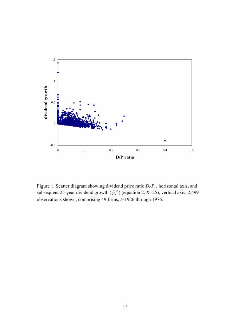
Figure 1 shows a scatter diagram of for K =25 against DDtg t /Pt for all 2,499
observations, that is for all 49 firms and for t=1926 to 1976 (1976 being the last year for
which 25 subsequent years are available). The range of Dt /Pt is from 0.0 to 0.4—several
times as wide as the range of the dividend-price ratio for the aggregate stock market over
the sample period. Over this entire range, there is a distinct negative slope to the curve, as
11

the efficient markets theory would predict: firms with lower dividend-price ratios did
indeed have higher subsequent dividend growth, offering some evidence for micro
efficiency. Plots for K=10, 15, and 20 look very similar to Figure 1.
One should be cautious in interpreting this diagram, however. Note that by
construction all points lie on or above a line from (0,0) with a slope of minus one,
reflecting the simple fact that dividends cannot go below zero. The efficient markets
model and our assumption that dividends beyond K years into the future cannot be
forecasted instead says that the scatter should cluster around a line from (0,r-c) with a
slope of minus one, a line that lies above the other line and is parallel with it, where c is
the mean of the truncated portion of the present value formula, as well as any possible
survivorship bias. But our results are not guaranteed by construction. Indeed when the
scatter of points for the aggregated firms (corresponding to the third regressions, Panel C
in the table) is plotted, it lies above this line but does not have a negative slope.
This line from (0,0) with a slope of minus one is easily spotted visually as the
lower envelope of the scatter of points. Any observation of Dt /Pt that is followed by a
dramatic drop in dividends (to approximately zero for K years) will lie approximately on
this line. Some of the most visible points on the scatter represent such firms. For example,
the extreme right outlier on the scatter, representing Schlumberger Ltd. in 1931,
represents nothing more than a situation in which the firm attempted to maintain its
dividend level in spite of rapidly declining fortunes. Its stock price fell precipitously after
the 1929 crash, converting a roughly 8% dividend into a 40% dividend, which was cut to
zero in 1932, and held there for many years. This extreme case may be regarded as a
victory for the efficient markets model, in that it does show that the dividend-price ratio
12

predicts future dividend growth, though not the usual case we think of when we consider
market efficiency. It is plain from the fact that the points are so dense around the lower
envelope line, that much of the fit derives from firms whose dividends dropped sharply.
Another simple story is that of firms that pay zero dividends. Note that all firm-
year pairs with zero dividends can be seen arrayed next to the vertical axis, and that the
dividend growth for these firms tends to be higher than for the firms with non-zero
dividends, as the dynamic Gordon model would predict. Firms with zero dividends
showed higher dividend growth as measured by : the mean for the zero-dividend
observations is 0.149, which, is greater than r=0.064, possibly reflecting the selection
bias for surviving firms noted above. The fact that these points along the vertical axis
cluster above 0.064 might also be considered a sort of approximate victory for market
efficiency. Also note that even if we deleted these firms, there still is a pronounced
negative slope to the scatter. The predictive ability of the dynamic Gordon model is not
just due to the phenomenon of zero dividends.
Dtg D
tg
Even if we delete all observations of zero dividends, and look at dividend price
ratios less than the discount rate r, that is, less than 0.064, then the slope of the regression
line for K=25 changes to –0.479, not much closer to zero. This means that there are also
observations of a low but non-zero dividend-price ratio successfully predicting above-
normal dividend growth.
Regression diagnostics following Belsley, Kuh and Welsch [1980] revealed that
no particularly influential observations were responsible for the results in the pooled
regressions.
13

Summary
With these data on the universe of U. S. individual firms on the CRSP tape with
continuous data since 1926 Samuelson’s dictum appears to have some validity. Over the
interval of U. S. history since 1926, individual-firm dividend-price ratios have had some
significant predictive power for subsequent growth rates in real dividends: this is
evidence of micro-efficiency. A look at a scatter plot of the data confirms that this result
is not exclusively due to zero dividends. Moreover, when the 49 firms are aggregated into
an index, the dividend-price ratio gets the wrong sign in the regressions, and is usually
insignificant. If anything, high aggregate dividend-price ratios predict high aggregate
dividend growth, and so there is no evidence of macro efficiency.11
The very negative results on the efficiency of the stock market that were reported
by LeRoy and Porter [1981] and Shiller [1981] appear to apply much more to the
aggregate stock market than to individual stocks.
11. The results are consistent with those of Vuolteenaho (2002), who uses firm-level data in conjunction with a vector autoregressive model and a variance decomposition along lines first described in Campbell [1991] to conclude that firm level stock returns are predominantly driven by fundamentals. Cohen, Polk and Vuolteenaho [2002] provide a similar variance decomposition of firm-level price to book ratios, finding that fundamentals predominate. Jung [2002] finds using variance and covariance ratio tests that individual stock returns show quite different mean reversion characteristics from the portfolio of them.
14
-0.5
0
0.5
1
1.5
0 0.1 0.2 0.3 0.4 0.5
D/P ratio
divi
dend
gro
wth
Figure 1. Scatter diagram showing dividend price ratio Dt/Pt , horizontal axis, and subsequent 25-year dividend growth ( ) (equation 2, K=25), vertical axis, 2,499 observations shown, comprising 49 firms, t=1926 through 1976.
Dtg
15

Table 1. Results of Regressions of Future Dividend Growth on Current Dividend-Price Ratio: ttt
Dt PDg εβα ++= )/(ˆ
Coefficient
of Dt/Pt
T statistic
R squared
A. Average of 49 Separate Regressions i) K=10, n=66 each regression ii) K=15, n=61 each regression iii) K=20, n=56 each regression iv) K=25, n=51 each regression
-0.440 -0.498 -0.490 -0.499
-2.11 -1.85 -1.67 -1.55
0.182 0.167 0.173 0.162
B. Pooled over all firms i) K=10, n=3,234 ii) K=15, n=2,989 iii) K=20, n=2,744
iv) K=25, n=2,499 v) K=75, n=49
-0.589 -0.648 -0.666 -0.711 -1.087
-5.91 -5.69 -4.82 -4.84 -1.41
0.174 0.217 0.216 0.149 0.041
C. Using the portfolio of the 49 firms i) K=10, n=66 ii) K=15, n=61 iii) K=20, n=56 iv) K=25, n=51
0.336 0.322 0.463 0.697
1.79 1.52 1.84 2.40
0.084 0.063 0.101 0.175
16

References
Belsley, David A., Edwin Kuh, and Roy E. Welsch, Regression Diagnostics: Identifying
Influential Data and Sources of Collinearity, New York: Wiley, 1980. Campbell, John Y. “A Variance Decomposition for Stock Returns,” Economic Journal,
101:157-79, 1991. Campbell, John Y. and Motohiro Yogo, “Efficient Tests of Stock Return Predictability,”
unpublished paper, Harvard University, 2002. Campbell, John Y., and Robert J. Shiller, “The Dividend-Price Ratio and Expectations of
Future Dividends and Discount Factors,” Review of Financial Studies, 1:195-228, 1988(a).
Campbell, John Y., and Robert J. Shiller, “Stock Prices, Earnings, and Expected
Dividends,” Journal of Finance 43:661-76, 1988(b). Campbell, John Y., and Robert J. Shiller, “Valuation Ratios and the Long-Run Stock
Market Outlook,” Journal of Portfolio Management, Winter 1998, pp. 11-26. Campbell, John Y., and Robert J. Shiller, “Valuation Ratios and the Long-Run Stock
Market Outlook: An Update,” NBER Working Paper No. 8221, 2001, forthcoming in Richard Thaler, editor, Advances in Behavioral Finance II, New York: Sage Foundation: 2003.
Cohen, Randolph, Christopher Polk, and Tuomo Vuolteenaho. 2002. “The Value
Spread.” unpublished paper, Harvard Business School, 2002, forthcoming, Journal of Finance.
Elliott, Graham, and James H. Stock, “Inference in Time Series Regression when the
Order of Integration of a Regressor is Unknown,” Econometric Theory, 10:672-700, 1994.
Hansen, Lars P., and Robert J. Hodrick, “Forward Exchange Rates as Optimal Predictors
of Future Spot Rates: An Econometric Analysis,” Journal of Political Economy, 88:829-53, 1980.
Jung, Jeeman, “Efficiency and Volatility of Stock Markets: Mean Reversion Detected by
Covariance Ratios,” unpublished manuscript, 2002. LeRoy, Stephen, and Richard Porter, “The Present Value Relation: Tests Based on
Variance Bounds,” Econometrica, 49:555-74, 1981.
17

18
Poterba, James M., and Lawrence H. Summers, “Mean Reversion in Stock Prices:
Evidence and Implications,” Journal of Financial Economics, 22:26-59, 1988.
Samuelson, Paul A., “Summing Up on Business Cycles: Opening Address,” in Jeffrey C. Fuhrer and Scott Schuh, Beyond Shocks: What Causes Business Cycles, Boston: Federal Reserve Bank of Boston, 1998.
Shiller, Robert J., “Do Stock Prices Move Too Much to be Justified by Subsequent
Changes in Dividends?” American Economic Review, 71:421-36, 1981.
Shiller, Robert J., Irrational Exuberance, 2nd Edition, New York: Broadway Books, 2000. Vuolteenaho, Tuomo, “What Drives Firm-Level Stock Returns?” Journal of Finance,
57:233-64, 2002