One-Dimensional Optical Wave Turbulence: Experiment andTheory

Jason Lauriea,∗, Umberto Bortolozzob, Sergey Nazarenkoc, Stefania Residorib

aLaboratoire de Physique, Ecole Normale Supereiure de Lyon, 46 allee d’Italie, Lyon, 69007, FrancebINLN, Universite de Nice, Sophia-Antipolis, CNRS, 1361 route des Lucioles, 06560, Valbonne,

FrancecMathematics Institute, University of Warwick, Coventry CV4 7AL, United Kingdom

Abstract

We present a review of the latest developments in one-dimensional (1D) optical waveturbulence (OWT). Based on an original experimental setup that allows for the imple-mentation of 1D OWT, we are able to show that an inverse cascade occurs through thespontaneous evolution of the nonlinear field up to the point when modulational instabilityleads to soliton formation. After solitons are formed, further interaction of the solitonsamong themselves and with incoherent waves leads to a final condensate state dominatedby a single strong soliton. Motivated by the observations, we develop a theoretical de-scription, showing that the inverse cascade develops through six-wave interaction, andthat this is the basic mechanism of nonlinear wave coupling for 1D OWT. We describetheory, numerics and experimental observations while trying to incorporate all the dif-ferent aspects into a consistent context. The experimental system is described by twocoupled nonlinear equations, which we explore within two wave limits allowing for theexpression of the evolution of the complex amplitude in a single dynamical equation.The long-wave limit corresponds to waves with wave numbers smaller than the electri-cal coherence length of the liquid crystal, and the opposite limit, when wave numbersare larger. We show that both of these systems are of a dual cascade type, analogousto two-dimensional (2D) turbulence, which can be described by wave turbulence (WT)theory, and conclude that the cascades are induced by a six-wave resonant interactionprocess. WT predicts several stationary solutions (non-equilibrium and thermodynamic)to both the long- and short-wave systems, and we investigate the necessary conditions re-quired for their realization. Interestingly, the long-wave system is close to the integrable1D nonlinear Schrodinger equation (NLSE) (which contains exact nonlinear soliton so-lutions), and as a result during the inverse cascade, nonlinearity of the system at lowwave numbers becomes strong. Subsequently, due to the focusing nature of the nonlin-earity, this leads to modulational instability (MI) of the condensate and the formation ofsolitons. Finally, with the aid of the the probability density function (PDF) descriptionof WT theory, we explain the coexistence and mutual interactions between solitons andthe weakly nonlinear random wave background in the form of a wave turbulence lifecycle (WTLC).

Keywords: Nonlinear optics, liquid crystals, turbulence, integrability, solitons

Preprint submitted to Elsevier July 26, 2016

© 2012, Elsevier. Licensed under the Creative Commons Attribution-NonCommercial-NoDerivatives 4.0 Internationalhttp://creativecommons.org/licenses/by-nc-nd/4.0/

Contents

1 Introduction 3

2 The Experiment 72.1 Description of the Experimental Setup . . . . . . . . . . . . . . . . . . . . 72.2 The Evolution of the Light Intensity and the Inverse Cascade . . . . . . . 92.3 The Long Distance Evolution and Soliton Formation . . . . . . . . . . . . 102.4 The Probability Density Function of the Intensity . . . . . . . . . . . . . . 132.5 The Relation to Previous Studies of Optical Solitons . . . . . . . . . . . . 142.6 The Theoretical Model of the OWT Experiment . . . . . . . . . . . . . . 15

2.6.1 The Long-Wave Regime . . . . . . . . . . . . . . . . . . . . . . . . 162.6.2 The Short-Wave Regime . . . . . . . . . . . . . . . . . . . . . . . . 17

2.7 The Nonlinearity Parameter . . . . . . . . . . . . . . . . . . . . . . . . . . 172.8 The Hamiltonian Formulation . . . . . . . . . . . . . . . . . . . . . . . . . 172.9 The Canonical Transformation . . . . . . . . . . . . . . . . . . . . . . . . 19

3 Wave Turbulence Theory 223.1 Solutions for the One-Mode PDF: Intermittency . . . . . . . . . . . . . . 233.2 Solutions of the Kinetic Equation . . . . . . . . . . . . . . . . . . . . . . . 243.3 Dual Cascade Behavior . . . . . . . . . . . . . . . . . . . . . . . . . . . . 243.4 The Zakharov Transform and the Power-Law Solutions . . . . . . . . . . . 253.5 Locality of the Kolmogorov-Zakharov Solutions . . . . . . . . . . . . . . . 293.6 Logarithmic Correction to the Direct Energy Spectrum . . . . . . . . . . . 303.7 Linear and Nonlinear Times and The Critical Balance Regime . . . . . . . 303.8 The Differential Approximation and the Cascade Directions . . . . . . . . 313.9 Modulational Instability and Solitons in the Long-Wave Equation . . . . . 33

4 Numerical results and comparison with the experiment 384.1 The Numerical Method . . . . . . . . . . . . . . . . . . . . . . . . . . . . 384.2 The Long-Wave Equation . . . . . . . . . . . . . . . . . . . . . . . . . . . 40

4.2.1 The Decaying Inverse Cascade with Condensation . . . . . . . . . 404.2.2 The PDF of the light intensity . . . . . . . . . . . . . . . . . . . . 434.2.3 The k − ω Plots: Solitons and Waves . . . . . . . . . . . . . . . . . 434.2.4 Forced and Dissipated Simulations . . . . . . . . . . . . . . . . . . 52

4.3 The Short-Wave Equation . . . . . . . . . . . . . . . . . . . . . . . . . . . 58

5 Conclusions 63

6 Acknowledgements 64

Appendices 66

∗Corresponding authorEmail addresses: jason.laurie@ens-lyon.fr (Jason Laurie), umberto@gmail.com (Umberto

Bortolozzo), s.v.nazarenko@warwick.ac.uk (Sergey Nazarenko), stefania.residori@inln.cnrs.fr(Stefania Residori)

2

A The Canonical Transformation 66

B Details and Assumptions of Weak Wave Turbulence Theory 69B.1 The Weak Nonlinearity Expansion . . . . . . . . . . . . . . . . . . . . . . 70B.2 Equation for the Generating Functional . . . . . . . . . . . . . . . . . . . 72

C The Zakharov Transform 75

D Expansion of the Long-Wave Six-Wave Interaction Coefficient 76

E Locality of the Kinetic Equation Collision Integral 77

F Derivation of the Differential Approximation Model 79

G The Bogoliubov Dispersion Relation 80

H Non-Dimensionalization 81

I The Intensity Spectrum 82

Bibliography 84

3

1. Introduction

One-dimensional (1D) optical wave turbulence (OWT) is an extremely interestingphysical phenomenon whose importance arises from its intrinsic overlap with severalstrategic research areas. This interdisciplinary nature allows for the application of non-conventional approaches to familiar facts and routes. These areas include wave turbulence(WT), Bose-Einstein condensate (BEC) and lasing, integrable systems and solitons, and,on a more fundamental level, general turbulence, nonlinear optics, equilibrium and non-equilibrium statistical mechanics. A hierarchical diagram showing these areas and theirlinks to 1D OWT is shown in figure 1.

Optical Wave Turbulence Integrable systems, Solitons

Kinetic Theory

Strongly non−equilibrium Statistical Systems,

Wave Turbulence

fluxes through phase space Thermodynamics

Systems in or near statistical equilibrium,

Turbulence

1D Optical Wave Turbulence

Nonlinear Optics

Figure 1: Interconnections of 1D OWT with other research areas.

The main aspects and phenomena in 1D OWT which will be at the focus of thepresent review include:

• The inverse transfer of wave action (from short to long wave lengths), its relationto the BEC of light, and to WT as an active medium for lasing;

• The role of turbulent cascades (fluxes) versus thermodynamic potentials (temper-ature and chemical potential) in 1D OWT and in WT in general;

• The proximity to integrability, modulational instability (MI) and the generation ofsolitons;

• The coexistence, interactions and mutual transformations of random waves andsolitons: this constitutes the wave turbulence life cycle (WTLC) and the evolutiontowards a final single soliton state.

Since WT concepts are central for our review, we will begin by giving a brief intro-duction to WT. WT can be generally defined as a random set of interacting waves with

4

a wide range of wave lengths. WT theory has been applied to several physical systemsincluding water surface gravity and capillary waves in oceans [1, 2, 3, 4, 5, 6, 7, 8, 9, 10,11, 12, 13, 14, 15, 16]; internal, inertial, and Rossby waves in atmospheres and oceans[17, 18, 19, 20, 21, 22, 23, 24, 25]; Alfven waves in solar wind and interstellar turbulence[26, 27, 28, 29, 30, 31, 32, 33, 34, 35, 36, 37]; Kelvin waves on quantized vortex linesin superfluid helium [38, 39, 40, 41, 42, 43, 44, 45, 46]; waves in BECs and nonlinearoptics [47, 48, 49, 50, 51]; waves in fusion plasmas [52, 53, 54, 3]; and waves on vibrating,elastic plates [55]. A thorough and detailed list of examples where the WT approachhas been applied, from quantum to astrophysical scales, can be found in the recent book[56]. The most developed part of the WT theory assumes that waves have randomphases and amplitudes and that their interactions are weakly nonlinear [3, 56], in whichcase a natural asymptotic closure arises for the statistical description of WT. The mostfamiliar outcome of such a closure is the kinetic equation (KE) for the wave action spec-trum and its stationary solutions describing energy and wave action cascades throughscales called Kolmogorov-Zakharov (KZ) spectra [2, 3, 56]. It is the similarity of the KZspectra to the Kolmogorov energy cascade spectrum in classical three-dimensional (3D)Navier-Stokes turbulence that allows one to classify WT as turbulence. On the otherhand, in most physical applications, besides weakly nonlinear random waves there arealso strongly nonlinear coherent structures which, even when not energetically dominant,interact with the random wave component, i.e. by random-to-coherent and coherent-to-random transformations, which may provide a route to the turbulence sink via wavebreaking or wave collapses. In other words, together with the random weakly nonlinearwaves, the strongly nonlinear coherent structures are also a fundamentally importantpart of the WTLC [56].

Let us now discuss realizations of WT in optical systems. Very briefly, we defineOWT as the WT of light. As such, OWT is a subject within the more general nonlinearoptics field, dealing with situations involving the propagation of light in nonlinear mediawhich is fully or partially random. OWT is a niche area within the nonlinear optics field,and excludes a large section of the field, including systems fully dominated by strongcoherent structures, such as solitons. The term turbulence, is even more relevant forOWT because of the similarities between the nonlinear light behavior to fluid dynamics,such as vortex-like solutions [57, 58] and shock waves [59]. Although there have beennumerous theoretical and numerical studies of OWT [50, 60, 61, 62, 47], there have beenfew experimental observations to date [51]. OWT was theoretically predicted to exhibitdual cascade properties when two conserved quantities cascade to opposite regions ofwave number space [50]. This is analogous to two-dimensional (2D) turbulence, wherewe observe an inverse cascade of energy and a direct cascade of enstrophy [63, 64]. Inthe context of OWT, energy cascades to high wave numbers, while wave action cascadestowards low wave numbers [50, 60, 61, 62]. An interesting property of OWT is the inversecascade of wave action which in the optical context implies the condensation of photons- the optical analogue of BEC.

It is the BEC processes that make OWT an attractive and important setup to study.Experimental implementation of BEC in alkali atoms was first achieved in 1995, andsubsequently awarded the 2001 Nobel prize [65, 66]. This work involved developing asophisticated cooling technique to micro-Kelvin temperatures, in order to make the deBroglie wave length exceed the average inter-particle distance. This is known as the BECcondition. Photons were actually the first bosons introduced by Bose in 1924 [67], and

5

the BEC condition is easily satisfied by light at room temperature. However, there wasthe belief that optical BEC would be impossible, because of the fundamental differencebetween atoms, whose numbers are conserved, and photons which can be randomlyemitted and absorbed. However, there exist situations where light is neither emittednor absorbed, e.g. light in an optical cavity, reflected back and forth by mirrors [68], orby light freely propagating through a transparent medium. In the latter, the movementof photons to different energy states (specifically the lowest one corresponding to BEC)can be achieved by nonlinear wave interactions. The mechanism for these nonlinearwave interactions is provided by the Kerr effect which permits wave mixing. Moreover,the nonlinear interactions are crucial for the BEC of light, because no condensation ispossible in non-interacting 1D and 2D Bose systems.

When the nonlinearity of the system is weak, OWT can be described by weak WTtheory [3, 56], with the prediction of two KZ states in a dual cascade system. One aspectof OWT is that the nonlinearity of the system is predicted to grow in the inverse cascadewith the progression of wave action towards large scales. This will eventually lead to aviolation of the weak nonlinearity assumption of WT theory. The high nonlinearity at lowwave numbers will lead to the formation of coherent structures [50, 61, 47, 69, 70, 71]. InOWT this corresponds to the formation of solitons and collapses for focusing nonlinearity[51], or to a quasi-uniform condensate and vortices in the de-focusing case [47].

Experimentally, OWT is produced by propagating light through a nonlinear medium[72]. However, the nonlinearity is typically very weak and it is a challenge to make itoverpower the dissipation. This is the main obstacle regarding the photon condensa-tion setup in a 2D optical Fabry-Perot cavity, theoretically suggested in [68] but neverexperimentally implemented.

This brings us to the discussion of the exceptional role played by 1D optical systems.Firstly, it is in 1D that the first ever OWT experiment was implemented [51]. The keyfeature in our setup is to trade one spatial dimension for a time axis. Namely, we considera time-independent 2D light field where the principal direction of the light propagationacts as an effective time. This allows us to use a nematic liquid crystal (LC), whichprovides a high level of tunable optical nonlinearity [73, 74]. The slow relaxation timeof the re-orientational dynamics of the LC molecules is not a restriction of our setupbecause the system is steady in time. Similar experiments were first reported in [75],where a beam propagating inside a nematic layer undergoes a strong self-focusing effectfollowed by filamentation, soliton formation and an increase in light intensity. Recently,a renewed interest in the same setup has led to further studies on optical solitons and theMI regime [76, 77, 78]. However, all the previous experiments used a high input intensity,implying a strong nonlinearity of the system, and therefore the soliton condensate appearsimmediately, bypassing the WT regime. In our experiment, we carefully set up an initialcondition of weakly nonlinear waves situated at high wave numbers from a laser beam.We randomize the phase of the beam, so that we produce a wave field as close to arandom phase and amplitude (RPA) wave field as possible. The nonlinearity of thesystem is provided by the LC, controlled by a voltage applied across the LC cell. Thisprovides the means for nonlinear wave mixing via the Kerr effect. The LC we use is of afocusing type, causing any condensate that forms to become unstable and the formationof solitons to occur via MI.

Secondly, from the theoretical point of view 1D OWT is very interesting because itrepresents a system close to an integrable one, namely the 1D nonlinear Schrodinger

6

equation (NLSE). Thus it inherits many features of the integrable model, e.g. thesignificant role of solitons undergoing nearly elastic collisions. On the other hand, de-viations from the integrability are important, because they upset the time recursions ofthe integrable system thereby leading to turbulent cascades of energy and wave actionthrough scales. We show that the process responsible for such cascades is a six-waveresonant interaction (wave mixing). Another example of a nearly integrable 1D six-wavesystem can be found in superfluid turbulence - it is the WT of Kelvin waves on quan-tized vortex lines [39, 79, 42, 43, 44, 46] (even though non-local interactions make thesix-wave process effectively a four-wave one in this case). Some properties of the six-wavesystems are shared with four-wave systems, particularly WT in the Majda-McLaughlin-Tabak (MMT) model reviewed in Physical Reports by Zakharov et al [71]. For example,both the four-wave and the six-wave systems are dual cascade systems, and in both sys-tems solitons (or quasi-solitons) play a significant role in the WTLC. There are alsosignificant differences between these two types of systems. Notably, pure KZ solutionsappear to be much less important for the six-wave optical systems than for the four-waveMMT model - instead the spectra have a thermal component which is dominant over theflux component. Moreover, the number of solitons in 1D OWT decrease in time due tosoliton mergers, so that asymptotically there is only a single strong soliton left in thesystem.

Similar behavior was extensively theoretically studied in various settings for non-integrable Hamiltonian systems starting with the paper by Zakharov et al [80], and thensubsequently in [81, 82, 83, 84, 85, 86, 87, 88, 89, 90]. The final state, with a singlesoliton and small scale noise, was interpreted as a statistical attractor, and an analogywas pointed out to the over-saturated vapor system, where the solitons are similar todroplets and the random waves behave as molecules [90]. Indeed, small droplets evaporatewhilst large droplets gain in size from free molecules, resulting in a decrease in the numberof droplets. On the other hand, in the 1D OWT context, the remaining strong soliton isactually a narrow coherent beam of light. This allows us to interpret the WT evolutionleading to the formation of such a beam as a lasing process. Here, the role of an activemedium where the initial energy is stored is played by the weakly nonlinear random wavecomponent, and the major mechanism for channeling this energy to the coherent beamis provided by the WT inverse cascade. For this reason, we can call such a system aWT laser. It is quite possible that the described WT lasing mechanism is responsiblefor spontaneous formation of coherent beams in stars or molecular clouds, although itwould be premature to make any definite claims about this at present.

Generally, in spite of recent advances, the study of 1D OWT is far from being com-plete. The present review provides a report on the current state of this area describingnot only what we have managed to learn and explain so far, but also the results which wedo not know yet how to explain, discussing the existing theory and the gaps within it thatare yet to be filled. We compare the experimental observations with the predictions ofWT theory and independently juxtapose our findings with direct numerical simulation ofthe governing equations. In particular, we describe some puzzles related to the wave ac-tion spectra obtained in the experiment and in the numerical experiments. Furthermore,we will describe the recent extensions of weak WT theory onto the wave probability den-sity function (PDF), which marks the beginning of developing a formalism for describingWT intermittency and the role of coherent structures. On the other hand, a theory forthe WTLC incorporating interacting random waves and coherent structures/solitons is

7

still to be investigated, with only of a few pioneering works reporting on the study of theinteraction between coherent structures and the radiating background [91].

2. The Experiment

The 1D optical system has been designed to meet the major requirements of OWT.Especially important are the careful calibrations that have been taken to fulfill the bal-ance between low dissipation and low nonlinearity. Indeed, the main experimental chal-lenge in observing the WT regime is in keeping the nonlinearity weak enough to let theWT regime develop and, at the same time, high enough to make it overpower the dissi-pation. Our setup is based on a nematic liquid crystal layer in which a laminar shapedbeam propagates. LCs are particularly suitable for the observation of the WT regime be-cause of their well known optical properties, such as their high and tunable nonlinearity,transparency (slow absorption) over a wide range of optical wave lengths, the realizationof large cells and the possibility to drive them with low voltage externally applied fields[74].

2.1. Description of the Experimental Setup

The liquid crystal, LC, cell is is schematically depicted in figure 2. It is made bysandwiching a nematic layer, (E48), of thickness d = 50 µm, between two 20 × 30mm2, glass windows and on the interior, the glass walls are coated with indium-tin-oxidetransparent electrodes. We have pre-treated the indium-tin-oxide surfaces with polyvinyl-alcohol, polymerized and then rubbed, in order to align all the molecules parallel to theconfining walls. When a voltage is applied across the cell, LC molecules tend to orientatein such a way as to become parallel to the direction of the electric field. By applying a 1kHz electric field with a rms voltage of V0 = 2.5 V we preset the molecular director toan average tilt angle Θ.

Vkz

E

Q

y

z

Figure 2: Schematic of the LC cell: molecules, initially aligned parallel to the confining walls, areoriented, through the application of the external voltage V , at an average angle θ, around which furtherreorientations are induced by the optical field ~E.

The experimental apparatus is shown in figure 3. It consists of a LC cell, insidewhich a laminar shaped beam propagates. An important point is that the input beamis carefully prepared in such a way as to have an initial condition of weakly nonlinearrandom waves. As depicted in figure 3a, the preparation of the input beam is such thatthe system is forced with an initial condition Qin, which is at a intermediate spatialscale between the large scale, k = 0, and the dissipative scale, kd. Moreover, phases

8

are randomized so that a narrow bandwidth forcing is realized around the initial spatialmodulation at the chosen wave number kin.

The setup is schematically represented in figure 3b. The input light originates froma diode pumped, solid state laser, with λ = 473 nm, polarized along y and shaped as athin laminar Gaussian beam of 30 µm thickness. The input light intensity is kept verylow, with an input intensity of I = 30 µW/cm2 to ensure the weakly nonlinear regime.A spatial light modulator (SLM), at the entrance of the cell is used to produce suitableintensity masks for injecting random phased fields with large wave numbers. This ismade by creating a random distribution of diffusing spots with the average size ' 35 µmthrough the SLM.

The beam evolution inside the cell is monitored with an optical microscope and a CCDcamera. The LC layer behaves as a positive uni-axial medium, where n‖ = nz = 1.7 isthe extraordinary refractive index and n⊥ = 1.5 is the ordinary refractive index [74].The LC molecules tend to align along the applied field and the refractive index, n(Θ),follows the distribution of the tilt angle θ. When a linearly polarized beam is injectedinto the cell, the LC molecules orientate towards the direction of the incoming beampolarization, thus, realizing a re-orientational optical Kerr effect. Because the refractiveindex increases when molecules orient themselves towards the direction of the input beampolarization, the sign of the nonlinear index change is positive, hence, we have a focusingnonlinearity.

Figure 3: a) Spatial forcing realized as initial condition Qin by appropriate preparation of the inputbeam; kin is the chosen wave number around which random phase modulations are introduced. b)Sketch of the experimental setup: a laminar shaped input beam propagates inside the LC layer; randomphase modulations are imposed at the entrance of the cell by means of a spatial light modulator, SLM.

Figure 4 depicts in more detail how the input light beam is prepared before enteringthe LC cell. The beam is expanded and collimated through the spatial light filter shownin figure 4. The objective, OB, focuses the light into the 20 µm pinhole, PH, the lensL1 collimates the beam with a waist of 18 mm. After that, the light passes through theSLM, which is a LCD screen working in transmission with a resolution of 800×600, with8 bits pixels, of size 14 µm. Each pixel is controlled through a personal computer PC,to ensure that the outgoing light is intensity modulated. In our case we use a cosinusmodulation having a colored noise envelope. The lenses, L3 and L4, are used to focus

9

the image from the LCD screen at the entrance of the LC cell. The half wave-plate,W, together with the polarizer, P, are used to control the intensity and the polarization,which is linear along the y-axis. The circular aperture is inserted in the focal plane tofilter out the diffraction given by the pixelization of the SLM and the diffuser, PH, isinserted to spatially randomize the phase of the light. In order to inject the light insidethe LC cell, we use a cylindrical lens, L4, close to the entrance of the LC layer.

Figure 4: Detailed representation of the experimental setup, showing the initialization of the input laserbeam. OB: objective, P1: pinhole, L1, L2, L3, L4: lenses, SLM: spatial light modulator, PC: computer,A: variable aperture, PH: random phase plate, W: half-wave plate, P: polarizer, LC: liquid crystals.

2.2. The Evolution of the Light Intensity and the Inverse Cascade

The inverse cascade can be observed directly in the experiment by inspecting the lightpattern in the (x, z) plane of the LC cell. Recall that z has here the role of time. Twomagnified images of the intensity distribution I(x, z) showing the beam evolution duringpropagation in the experiment are displayed in figure 5. For comparison, in figure 5aand b, we show the beam evolution in the linear and in the weakly nonlinear regimes,respectively. In figure 5a, we set a periodic initial condition with a uniform phase andapply no voltage to the LC cell. We see that the linear propagation is characterized bythe periodic recurrence of the pattern with the same period, a phase slip occurring atevery Talbot distance. This is defined by p2/λ, with p, the period of the initial conditionand λ, the laser wave length [92]. In figure 5b, we apply a voltage, V = 2.5 V to the LCcell. The initial condition is periodic with the same period as in figure 5a, but now withrandom phases. We observe that the initial period of the pattern is becoming larger asthe light beam propagates along z.

While the linear propagation in figure 5a, forms Talbot intensity carpets [93], withthe initial intensity distribution reappearing periodically along the propagation directionz, the weak nonlinearity in figure 5b, leads to wave interactions, with different spatialfrequencies mixing and the periodic occurrence of the Talbot carpet being broken. Infigure 6, we show two intensity profiles taken in the nonlinear case at two different stagesof the beam propagation. The inverse cascade is accompanied by a smoothing of theintensity profile and the amplification of low wave number components.

The inverse cascade can be measured directly by recording the evolution of the trans-verse light pattern I(x, z) along z. However, experimentally we measure the light inten-sity I(x, z) as we do not have direct access to the phases. Therefore, we measure the

10

Figure 5: Intensity distribution I(x, z) showing the beam evolution during propagation; a) linear case(no voltage applied to the LC cell), b) weakly nonlinear case (the voltage applied to the LC cell is setto 2.5 V ). d is the spatial period of the input beam modulation at the entrance plane of the cell.

spectrum of intensity N(k, z) = |Ik(z)|2, for which an appropriate scaling should be de-rived from the theory. The experimental scaling for Nk in the inverse cascade is obtainedby fitting the experimental spectrum of the light intensity, and gives Nk ∼ |k|−1/5 asshown in figure 7. One can see an inverse cascade excitation of the lower k states, and agood agreement with the WT prediction.

[>PP@

,>DX@

] PP] PP

Figure 6: Two intensity profiles I(x) recorded at z = 0 and z = 1.9 mm in the weakly nonlinear regime,with V = 2.5 V , showing the smoothing associated with the inverse cascade.

11

101 102

k [mm-1]

|Ik |2

z=0 mm

z=4.2 mm

k -1/5

100

Figure 7: Experimental spectrum of the light intensity, Nk = |Ik|2 at two different distances z.

2.3. The Long Distance Evolution and Soliton Formation

The intensity distribution I(x, z), showing the beam evolution during propagationfor longer distances is displayed in figures 8. In the high resolution inset we can observethat the typical wavelength of the waves increases along the beam, which corresponds toan inverse cascade process. Furthermore, one can see the formation of coherent solitonsout of the random initial wave field, such that in the experiment, one strong soliton isdominant at the largest distance z.

0.5

1.0

0

x [

mm

]

z [mm]2 4 6 8

Figure 8: Experimental results for intensity distribution I(x, z). The area marked by the dashed line isshown at a higher resolution (using a larger magnification objectif).

12

-0.4 -0.2 0 0.2 0.40.40

1000

2000

3000

4000

0.3 mm4.5 mm

7.5 mm

x [mm]

I (g

ray

val

ues

)

Figure 9: Linear intensity profiles I(x) taken at different propagation distances, z = 0.3, 4.5 and 7.5mm.

The experimental evolution reported in figure 8 indicates that the total number ofsolitons reduces. The observed increase of the scale and formation of coherent structuresrepresents the condensation of light. Experimentally, the condensation into one domi-nant soliton is well revealed by the intensity profiles I(x) taken at different propagationdistances, as shown in figure 9 for z = 0.3, 4.5 and 7.5 mm. Note that the amplitude ofthe final dominant soliton is three orders of magnitude larger than the amplitude of theinitial periodic modulation.

0 1 2 3 4 5 6 7 80.8

0.85

0.9

0.95

1

z (mm)

<I>/Iin

inverse cascade

solitons

Figure 10: Evolution of the normalized x-averaged light intensity < I > /Iin, where Iin is the inputintensity, as a function of the propagation distance z.

As for energy dissipation, we should note that this is mainly due to radiation losses,whereas absorption in the liquid crystals is practically negligible [94]. In order to give

13

an estimation of the losses occurred during the z evolution we have averaged the lightintensity I(x, z) along x and calculated the ratio of the x-averaged intensity < I > tothe input intensity Iin. The result is plotted in figure 10, from which we observe thatafter 8 mm of propagation the losses are about 15%. Moreover, by comparing figure 10with the intensity distribution I(x, z) (see figure 8), we can note that during the inversecascade the total light intensity remains practically constant, whereas losses become moreimportant when solitons start to appear.

2.4. The Probability Density Function of the Intensity

0 2000 4000 6000

0.01

0.1

1

I

p(I)

0 mm

3 mm

8 mm

Figure 11: PDFs of the wave intensity within the experimental cell at three different distances along thecell, z = 0 mm, z = 3 mm and z = 8 mm. Straight lines correspond to the Rayleigh PDF’s correspondingto Gaussian wave fields (these fits have the same mean as the respective numerical PDFs).

Figure 11 displays three experimentally obtained profiles of the PDF of the waveintensity along the cell at distances z = 0 mm, z = 3 mm and z = 8 mm in lin-logcoordinates. In a pure Gaussian wave field, we would observe the Rayleigh distribution(31) which would correspond to a straight profile of the PDF in lin-log coordinates.However, in figure 11, non-Gaussianity is observed with the deviation from the straightlines, indicating a slower that exponential decay of the PDF tails. Non-Gaussianitycorresponds to intermittency of WT.

Intermittency implies that there is a significantly higher occurrence of high intensitystructures compared to that predicted by a Gaussian wave field and that the system isin the presence of an MI process leading to solitons. The observation of intermittencycould be a sign of the development of coherent structures (solitons) in the system.

Analogies can be drawn of such high amplitude solitons with the rogue waves ap-pearing in systems characterized by many nonlinearly interacting waves, as seen on theocean surface [95], in nonlinear optical systems [96, 97, 98], and in superfluids [99]. For

14

all of which a description in terms of nonlinear coherent structures emerging from mod-ulational instability in the nonlinear Schrodinger equation can been outlined [100]. Inparticular, possible links between rogue waves and wave turbulence in optical systemsare discussed in [101].

2.5. The Relation to Previous Studies of Optical Solitons

Optical re-orientation of the LC occurs under the action of the light itself, with the LCmolecules tending to align along the direction of the laser beam polarization, and givingrise to a Kerr effect that produces a self-focusing nonlinearity [73]. This effect was shownto lead to laser beam filamentation [75] and, recently, has been exploited to demonstratethe stable propagation of spatial optical solitons, also called nematicons, inside nematicLC cells [76]. For the same type of system, MI has also been reported [77, 78]. However,the previous experiments used a high input intensity, implying a strong nonlinearity ofthe system, and therefore filamentation and solitons appeared immediately, bypassingthe WT regime.

Solitons are well-known and widely studied in nonlinear optics [102], where they areunderstood as light pulses that maintain their shape, unaltered during propagation in anonlinear medium, and where the nonlinearity implies a change in the refractive indexthat is induced by the intensity of the light itself. In this context solitons are classified asbeing either spatial or temporal, whether the self-confinement of the light beam occurs inspace or in time during their propagation. The nonlinearity of the medium corresponds,respectively, to a self-focusing or a self phase modulation effect.

While WT implies the presence of many random waves interacting with low nonlinear-ity, previous work conducted in the nonlinear optics field was mainly aimed at realizingself-confined beams in a different regime, where the nonlinearity was relatively high andthe medium seeded by a single pulse of Gaussian shape. A spatial soliton is thereforeobtained by imposing a tightly focused beam as an initial condition and, then by lettingthe beam propagate inside a medium where the self-focusing nonlinearity compensatesthe transverse beam widening by diffraction. These types of spatial solitons have beenobserved in a number of diverse optical media, such as, photorefractive crystals, atomicvapors, and semiconductor wave guides [103, 104]. On the other hand, temporal solitonscorrespond to cases when the nonlinearity compensates the temporal broadening of alight pulse due to the natural dispersion of the traversed medium [74], and have beenobserved in optical fibers.

In both cases, the theoretical approach to spatial and the temporal solitons are basedon the NLSE. We therefore expect the generic behavior of the system to have an OWTregime existing before the formation of solitons. This entails an inverse cascade, thedevelopment of soliton turbulence and subsequently, a final single soliton acting as astatistical attractor of the system [80]. In the spatial case, the light propagation direction,usually denoted as z, plays the role of time, therefore the wave dispersion relation is ofthe type ω = k2, whereas in the temporal case the time derivative is in the secondorder dispersion term, hence the dispersion relation is of the type k = ω2. Theoreticalpredictions of OWT regimes should, therefore, be different in both cases. Recently,experiments achieving WT regimes in optical fibers have been devised [105] and thewave thermalization phenomena has been reported for the same type of system [106].

15

However, up to now only in the LC experiment has there been a genuine WT regime,with an inverse cascade and the spontaneous emergence of spatial solitons out of randomwaves, been demonstrated [51].

2.6. The Theoretical Model of the OWT Experiment

Theoretically, the experimental setup can be modeled by an evolution equation forthe input beam, coupled to a relaxation equation for the LC dynamics given by

2iq∂ψ

∂z+∂2ψ

∂x2+ k2

0n2aaψ = 0, (1a)

∂2a

∂x2− 1

l2ξa+

ε0n2a

4K|ψ|2 = 0, (1b)

where ψ(x, z) is the complex amplitude of the input beam propagating along the timeaxis z; x is the coordinate across the beam; a(x, z) is the LC reorientation angle; na =ne − no is the birefringence of the LC; k0 is the optical wave number; ε0 is the vacuumpermittivity; and lξ =

√πK/2∆ε(d/V0) is the electrical coherence length of the LC [107],

withK being the elastic constant, q2 = k20

(n2o + n2

a/2)

and ∆ε is the dielectric anisotropy.Note that lξ fixes the typical dissipation scale, limiting the extent of the inertial rangein which the OWT cascade develops. In other contexts, such a spatial diffusion of themolecular deformation has been denoted as a non-local effect, see [76, 77, 78]. In ourexperiment, when V0 = 2.5 V , we have that lξ = 9 µm. By considering that a typicalvalue of K is of the order ∼ 10 pN , we can derive a typical dissipation length scale ofthe order ∼ 10 µm.

The evolution equations, (1) for the complex amplitude of the input beam, ψ(x, z),to the LC reorientation angle, a(x, z) can be re-written as a single equation for fieldψ(x, z). This can be achieved by formally inverting the operator on a(x, z) in equation(1b). Equation (1b) implies that

a(x, z) =ε0n

2a

4K

(1

l2ξ− ∂2

∂x2

)−1

|ψ|2. (2)

Substituting this expression into equation (1a), we eliminate the dependence on variablea(x, z). This gives

2iq∂ψ

∂z+∂2ψ

∂x2+k2

0n4aε0

4Kψ

(1

l2ξ− ∂2

∂x2

)−1

|ψ|2 = 0. (3)

Equation (3) is a single equation modeling the evolution of the complex amplitude,ψ(x, z). We can further simplify equation (3) by considering the system in two limitsof wave number k: klξ 1 and 1 klξ, that we call the long- and short-wave limitsrespectively. These limits enable the expansion of the nonlinear operator in power oflξ∂/∂x. Our experimental system is well described by the long-wave limit. The limita-tions imposed by the dissipation of the LC in the current experimental setup preventsthe implementation in the short-wave regime. However, for the completeness of our de-scription and for the possibilities in the modification of the experimental setup in thefuture for the short-wave regime, we will continue to investigate this limit theoreticallyand numerically.

16

2.6.1. The Long-Wave Regime

The long-wave approximation to equation (3) corresponds to the wavelength of thespatial light distribution, λ ∝ 1/k, being greater than the electrical coherence length ofthe LC, lξ. In physical space, this limit corresponds to lξ∂/∂x 1, which permits theexpansion of the nonlinear operator of equation (3) as(

1

l2ξ− ∂2

∂x2

)−1

= l2ξ

(1 + l2ξ

∂2

∂x2+ l4ξ

∂4

∂x4+ · · ·

). (4)

Taking the leading order of this expansion yields

2iq∂ψ

∂z= −∂

2ψ

∂x2− 1

2l2ξ ψ2ψ|ψ|2 (5)

where, for clarity, we have introduced a reference light intensity:

ψ2 =2K

ε0n4al

4ξk

20

. (6)

Equation (5) is the 1D focusing NLSE. As is well-known, the 1D NLSE is an integrablesystem, solvable with the aid of the inverse scattering transform [108], and characterizedby solitons 1. Unfortunately, this would be a poor model for OWT, as the integrabilityof the 1D NLSE implies that wave turbulent interactions are not possible. To overcomethis, we must consider the sub-leading contribution in expansion (4). This extra nonlinearterm acts as a correction breaking the integrability of the system. The resulting equationis given as

2iq∂ψ

∂z= −∂

2ψ

∂x2− 1

2l2ξ ψ2

(ψ|ψ|2 + l2ξψ

∂2|ψ|2

∂x2

). (7)

We refer to equation (7) as the long-wave equation (LWE). For the expansion (4) to bevalid, the additional nonlinear term must be considered smaller than the leading nonlinearterm. Moreover for OWT to be in the weakly nonlinear regime, both of the nonlinearcontributions should be smaller than the linear term. Therefore, although integrabilityis lost, the system will remain close to the integrable one described by (5). As a result,we expect soliton-like solutions close to the exact solutions of the 1D NLSE (5). On theother hand, exact soliton solutions of equation (5), do not change shape, and have theability to pass through one another unchanged. We can expect that in the LWE (7),we will observe similar soliton solutions, but the non-integrability will allow solitons tointeract with one another, and with the weakly nonlinear random wave background.

2.6.2. The Short-Wave Regime

In the opposite limit of equation (3), when 1 l2ξ∂2/∂x2, the nonlinear operator of

equation (3) can be represented in terms of a Taylor expansion of negative powers of the

1The term soliton is sometimes reserved for solitary waves with special properties arising from inte-grability, such as the ability to pass through one another without change in shape or velocity, as is thecase for the 1D NLSE. Hereafter, we will use the term soliton more broadly, including solitary waves innon-integrable systems which can change their states upon mutual collisions.

17

spatial derivative:(1

l2ξ− ∂2

∂x2

)−1

= −(∂2

∂x2

)−1

+1

l2ξ

(∂2

∂x2

)−2

− · · · . (8)

It is sufficient for us to approximate the nonlinear operator of equation (3) with justthe leading order term in expansion (8), as integrability of the equation is not an issue.Therefore, we get an equation of the form:

2iq∂ψ

∂z= −∂

2ψ

∂x2+

1

2l4ξ ψ2ψ

(∂2

∂x2

)−1

|ψ|2. (9)

We call equation (9) the short-wave equation (SWE). Ultimately, we have presentedtwo dynamical equations for the complex wave amplitude ψ(x, z) for 1D OWT in twolimits of wave number space. Both of these systems can be expressed in a Hamiltonianformulation, that will be utilized by WT theory in the weakly nonlinear regime.

2.7. The Nonlinearity Parameter

It is essential for the development of OWT that the system operates in a weaklynonlinear regime. We can quantify the linearity and nonlinearity within the system withthe introduction of a nonlinear parameter, J , which is determined by the ratio of thelinear term to the nonlinear term within the dynamical equations.

For instance, the nonlinear parameter from the LWE (7) is defined as

JL =2ψ2k2l2ξ

I. (10)

This is derived from the ratio of the linear term and the first of the two nonlinear terms.Here, I =

⟨|ψ(x, z)|2

⟩is the average value of the light intensity. Similarly, the SWE, (9)

yields a nonlinearity parameter of

JS =2ψ2k4l4ξ

I. (11)

Calculation of JL and JS act as a verification of the weak nonlinear assumption ofWT. This is especially important in the context of experimental implementations ofOWT, where initially unknown quantities are often difficult to measure.

2.8. The Hamiltonian Formulation

Both equations (7) and (9) can be written in terms of a Hamiltonian system of theform

2iq∂ψ

∂z=

δHδψ∗

. (12)

For the LWE, the Hamiltonian is given as

HL = H2 +HL4 ,

=

∫ ∣∣∣∣∂ψ∂x∣∣∣∣2 − 1

4ψ2

[|ψ|4

l2ξ−(∂|ψ|2

∂x

)2]

dx. (13a)

18

In the nonlinear energy term H4, the term quartic with respect to ψ, we have addeda superscript L to denote that this quartic term corresponds to the LWE, (7). This isbecause the Hamiltonian of the LWE and SWE only differ in the expression H4. For theSWE, the Hamiltonian is given by

HS = H2 +HS4 ,

=

∫ [∣∣∣∣∂ψ∂x∣∣∣∣2 − 1

4l4ξ ψ2

(∂−1|ψ|2

∂x−1

)2]dx. (13b)

In both the LWE and the SWE, the linear, (quadratic), energy H2 is identical. TheHamiltonians (13) coincide with the total energy of the systems and are conserved bytheir respective dynamics (H = const). Moreover, both the LWE and SWE contain anadditional invariant, the wave action N defined as

N =

∫|ψ|2dx. (14)

Conservation of N is a consequence of the U(1) gauge symmetry or invariance of equa-tions (7) and (9) with respect to a phase shift: ψ(x, z)→ ψ(x, z) exp (iφ).

By expressing the Hamiltonian in terms of its Fourier representation

ψ(x, z) =∑k

a(k, z)eikx, (15)

here k ∈ R, the general Hamiltonian structure for Hamiltonians (13) can be representedin terms of the wave amplitude variable:

H =∑k

ωk aka∗k +

1

4

∑1,2,3,4

T 1,23,4 a1a2a

∗3a∗4 δ

1,23,4 , (16)

where ωk = k2 is the linear frequency2 of non-interacting waves, δ1,23,4 = δ(k1 + k2− k3−

k4) is a Kronecker delta function, T 1,23,4 = T (k1,k2,k3,k4) is the nonlinear interaction

coefficient, and the subscripts in the summation correspond to the summation over theassociated wave numbers. Note that we use bold symbol k for the wave number toemphasize that it can be either positive or negative, while k is reserved specifically forthe wave vector length, k = |k|.

By symmetry arguments, the interaction coefficient should not change under thepermutations k1 ↔ k2, k3 ↔ k4. Furthermore, the Hamiltonian (16) represents thetotal energy of the system and is therefore a real quantity. This property implies extrasymmetries of the interaction coefficient:

T 1,23,4 = T 2,1

3,4 = T 1.24,3 = (T 3,4

1,2 )∗. (17)

For the LWE Hamiltonian (13a), the interaction coefficient is defined as follows,

LT 1,23,4 = 1T 1,2

3,4 + 2T 1,23,4

= − 1

l2ξ ψ2

+1

2ψ2(k1k4 + k2k3 + k2k4 + k1k3 − 2k3k4 − 2k1k2) . (18a)

2Indeed, ωk is the frequency with respect to the time variable which is related to the distance z ast = z/2q.

19

We have denoted the two contributions to LT 1,23,4 , from both nonlinear terms in (7), as

1T 1,23,4 and 2T 1,2

3,4 , where the first arises from the usual cubic nonlinearity seen in the 1Dfocusing NLSE, and the second from the sub-leading correction.

Similarly, the SWE yields the following interaction coefficient,

ST 1,23,4 =

1

2l4ξ ψ2

(1

k1k3+

1

k2k3+

1

k1k4+

1

k2k4− 2

k1k2− 2

k3k4

). (19a)

In terms of the wave amplitude variables a(k), the Hamiltonian system (16) satisfies theFourier space analogue of equation (12):

2iq∂a(k, z)

∂z=

δHδa∗(k, z)

. (20)

It is with equation (20) that the formulation of WT theory is applied. In the nextSection, we will give a brief mathematical description of WT theory, and outline theassumptions on the wave field that is required to apply such an approach.

2.9. The Canonical Transformation

Nonlinear wave interactions can be classified by the lowest order of resonance interac-tions they undergo. For an N ↔M wave scattering process, these resonance conditionsare defined as

k1 + · · ·+ kN = kN+1 + · · ·+ kN+M , (21a)

ω1 + · · ·+ ωN = ωN+1 + · · ·+ ωN+M , (21b)

where ki is the wave number and ωi = ω(ki) is the frequency of wave i.The lower orders of nonlinearity can be eliminated using a quasi-identity canoni-

cal transformation (CT) which is similar to the Poincare-type algorithm used in, e.g.the construction of the corrected wave action for the perturbed integrable systems inKolmogorov-Arnold-Moser (KAM) theory. The latter represents a recursive procedureeliminating the lower-order interaction terms one by one at each of the recursive steps,which is only possible when there are no resonances at that respective order. In WT the-ory, such a recursion is “incomplete” - it contains a finite number of recursive steps untilthe later steps are prevented by the lowest order wave resonances. The CT procedurefor eliminating the non-resonant interactions in WT theory is explained in [3], where themost prominent example given was for the system of gravity water waves, where it wasused to eliminate the non-resonant cubic Hamiltonian (see also [109] where some minormistakes made for gravity waves were corrected).

Of course, apart for satisfying the resonant conditions, the respective type of the non-linear coupling must be present. For example, the 2D and 3D NLSE have the dispersionrelation ωk = k2 which can satisfy the three-wave 1 ↔ 2 resonance conditions, but thethree-wave nonlinear coupling is zero. On the other hand, for gravity water waves thereis a 1↔ 2 wave interaction Hamiltonian (when written in terms of the natural variables- height and velocity potential), but the wave linear frequency ωk =

√gk does not allow

for 1 ↔ 2 resonances [52]. As a consequence, the lowest order resonant processes in allof these cases are four-wave (2 ↔ 2). For 1D OWT, like in the NLSE, the frequency ofthe linear propagating waves is given by

ω(k) = k2, (22)20

k

ω1

ω3

ω1 + ω2= ω3 + ω4

ω1 = ω3ω1 + ω2ω3 + ω4

k1 k2

k3 k4

0

Figure 12: We plot a graphical representation of the four-wave resonance condition [56]. The four-wave resonance condition is satisfied at points where the green and blue lines intersect, (shown by theblack dot). However, for dispersion relations ωk ∝ kα, with α > 1, there can only be one intersection,corresponding to the trivial wave resonance: k1 = k4 and k2 = k3.

In 1D, dispersion relations of the form ω(k) ∝ kα with α > 1 cannot satisfy the four-waveresonance condition:

k1 + k2 = k3 + k4, (23a)

ω(k1) + ω(k2) = ω(k3) + ω(k4). (23b)

This can be understood by a simple graphical proof presented in figure 12 [56]. Infigure 12 we observe the red dashed curve representing the dispersion relation ωk = Ckα

with α > 1. At two locations along this curve (at k = k1 and k = k3), two furtherdispersion curves (the green and blue solid lines) are produced: with their minima atpoints (k, ω) = (k1, ω1) and at (k3, ω3) respectively. These subsequent lines represent thewave frequencies of ω1 +ω2 and ω3 +ω4, where k1 and k3 are now fixed, with k2 varyingalong the green solid line and k4 varying along the blue line. If the green and blue linesintersect, it will be when the four-wave resonance condition (23) is satisfied and will occurat the point (k, ω) = (k1 +k2, ω1 +ω2) = (k3 +k4, ω3 +ω4). In figure 12, we observe thatsuch an intersection occurs only once, and it can be clearly seen that k1 = k4 and k2 = k3

must hold. This corresponds to a trivial pairing of wave numbers, which will not provideany nonlinear energy exchange between modes. As a consequence, resonant four-waveinteractions are absent in the system. There are no five-wave interactions either becausethe U(1) symmetry prohibits the presence of odd orders in the wave amplitude in theinteraction Hamiltonian. In situations such as these, there exists a weakly nonlinear CTthat allows us to change to new canonical variables such that the leading interactionHamiltonian is of order six.

21

A similar strategy was recently applied to eliminate non-resonant fourth-order inter-actions in the context of Kelvin waves in superfluid turbulence [110, 44] and in nonlinearoptics [51]. The details of the CT for our optical system can be found in Appendix A. Theresult of the CT is the representation of our system in a new canonical variable ck withthe elimination of the quartic contribution H4. This however results in the appearanceof a sextic contribution H6 :

H =∑k

ωkckc∗k +

1

36

∑1,2,3,4,5,6

W1,2,34,5,6 δ

1,2,34,5,6 c1c2c3c

∗4c∗5c∗6, (24)

where the explicit formula for W1,2,34,5,6 stemming from the CT is given by

W1,2,34,5,6 = −1

8

3∑i,j,m=1i 6=j 6=m6=i

6∑p,q,r=4p 6=q 6=r 6=p

T p+q−i,ip,q T j+m−r,rj,m

ωj+m−r,rj,m

+T i+j−p,pi,j T q+r−m,mq,r

ωq+r−m,mq,r

, (25)

where we have use the notation ω1,23,4 = ω1 + ω2 − ω3 − ω4. Note that analogous to the

symmetries of the four-wave interaction coefficient T 1,23,4 , we must similarly impose the

following symmetry conditions on W 1,2,34,5,6 to ensure the Hamiltonian is real:

W1,2,34,5,6 =W2,1,3

4,5,6 =W3,2,14,5,6 =W1,3,2

4,5,6 =W2,3,14,5,6 =W3,1,2

4,5,6 =(W4,5,6

1,2,3

)∗. (26)

Hamiltonian (24) represents the the original Hamiltonian system (16), but now in thenew canonical variable ck. The interaction Hamiltonian has now been transformed fromhaving a leading non-resonant fourth-order interaction term into one with a leading res-onant six-wave interaction. From the formula of the new six-wave interaction coefficient(25), the six-wave interaction stems from the coupling of two non-resonant four-waveinteractions connected by a virtual wave (an illustration is presented in figure 13).

By substituting Hamiltonian (24) into equation (20), we derive an evolution equationfor the wave action variable ck,

ick = ωkck +1

12

∑2,3,4,5,6

Wk,2,34,5,6 c∗2c

∗3c4c5c6 δ

k,2,34,5,6 , (27)

where we denote the “time” derivative of ck as ck = ∂ck/∂z. This equation is the startingpoint for WT theory. This is the six-wave analogue of the well-known Zakharov equationdescribing four-wave interactions of water surface waves [111].

3. Wave Turbulence Theory

General formulation of WT theory can be found in a recent book [56], reviews [112,71, 113] and the older classical book [3]. In our review will will only outline the basicideas and steps of WT, following mostly the approach of [56]. More details will be givenon the parts not covered in these sources, namely the six-wave systems arising in OWTand respective solutions and their analysis.

Let us consider a 1D wave field, a(x, z), in a domain which is periodic in the x-direction with period L, and let the Fourier transform of this field be represented by the

22

Figure 13: An illustration to show the non-resonant four-wave interaction, T 1,23,4 , and the resonant six-

wave interaction, W1,2,34,5,6 , after the CT. The six-wave (sextet) interaction term is a contribution arising

from two coupled four-wave (quartet) interactions via a virtual wave (dashed line).

Fourier amplitudes al(t) = a(kl, z), with wave number, kl = 2πl/L, l ∈ Z. Recall that thepropagating distance z in our system plays a role of “time”, and consider the amplitude-phase decomposition al(t) = Al(z)ψl(z), such that Al is a real positive amplitude andψl is a phase factor that takes values on the unit circle in the complex plane. Following[114, 115, 116, 117], we say a wave field a(x, z) is an RPA field, if all the amplitudes Al(z)and the phase factors ψl(z) are independent random variables and all ψls are uniformlydistributed on the unit circle on the complex plane. We remark, that the RPA propertydoes not require us to fix the shape of the amplitude PDF, and therefore, we can dealwith strongly non-Gaussian wave fields. This will be useful for the description of WTintermittency.

Construction of the WT theory for a particular wave system consists of three mainsteps: i) expansion of the Hamiltonian dynamical equation (equation (27) in our case)in powers of a small nonlinearity parameter, ii) making the assumption that the initialwave field is RPA and statistical averaging over the initial data, and finally iii) takingthe large box limit followed by the weak nonlinearity limit. Since the derivations for ourOWT example are rather technical and methodologically quite similar to the standardprocedure described in [56], we move these derivations to Appendix B. This approachleads to an evolution equation for the one-mode amplitude PDF Pk(sk) which is theprobability of observing the wave intensity Jk = |Ak|2 of the mode k in the range(sk, sk + dsk):

Pk = −∂Fk

∂sk, Fk = −

(skγkPk + skηk

∂Pk

∂sk

), (28)

where we have introduced a probability space flux Fk and where

ηk =ε8π

6

∫|Wk,2,3

4,5,6 |2 δk,2,34,5,6 δ(ωk,2,34,5,6 ) n2n3n4n5n6 dk2dk3dk4dk5dk6, (29a)

23

and

γk =ε8π

6

∫|Wk,2,3

4,5,6 |2 δk,2,34,5,6 δ(ωk,2,34,5,6 ) [(n2 + n3)n4n5n6

−n2n3 (n4n5 + n4n6 + n5n6)] dk2dk3dk4dk5dk6. (29b)

Multiplying equation (28) by sk and integrating over sk, we then obtain the KE, anevolution equation for the wave action density nk = 〈|ck|2〉:

nk = ηk − γknk, (30)

Our main focus is on the non-equilibrium steady state solutions of equations (28) and(30).

3.1. Solutions for the One-Mode PDF: Intermittency

The simplest steady state solution corresponds to the zero flux scenario, Fk = 0:

Phom =1

nke− sknk , (31)

where nk corresponds to any stationary state of the KE. Solution Phom, is the Rayleighdistribution. Subscript hom refers to the fact that this is the solution to the homogeneouspart of a more general solution for a steady state with a constant non-zero flux, Fk =F 6= 0. The general solution in this case is [114]

Pk = Phom + Ppart, (32)

where Ppart is the particular solution to equation (28). The particular solution is acorrection due to the presence of a non-zero flux. In the region of the PDF tail, wheresk nk, we can expand Ppart in powers of nk/sk:

Ppart = − Fskγk

− ηkF(skγk)

2 − · · · . (33)

Thus, at leading order, the PDF tail has algebraic decay ∼ 1/sk, which corresponds tothe presence of strong intermittency of WT [114]. From equation (33), we observe thata negative F implies an enhanced probability of high intensity events. Subsequently, apositive flux, F , would imply that there is less probability in observing high intensitystructures than what is expected by a Gaussian wave field. In WT systems, we expectto observe both kinds of behavior each realized in its own part of the k-space forming aWTLC, which will be discussed later.

3.2. Solutions of the Kinetic Equation

The KE (30) is the main equation in WT theory, it describes the evolution of thewave action spectrum nk. It can be written a more compact form as

nk =ε8π

6

∫|Wk,2,3

4,5,6 |2 δk,2,34,5,6 δ(ωk,2,34,5,6 ) nkn2n3n4n5n6

×(n−1k + n−1

2 + n−13 − n

−14 − n

−15 − n

−16

)dk2dk3dk4dk5dk6. (34)

24

The integral on the right hand side of the KE, (34), is known as the collision integral.Stationary solutions of the KE are solutions that make the collision integral zero. Thereexist two types of stationary solutions to the KE. The first type are referred to as thethermodynamic equilibrium solutions. The thermodynamic solutions correspond to anequilibrated system and thus refer to an absence of a k-space flux for the conservedquantities, (in our case, linear energy, H2, and total wave action, N ). The second typeare known as the KZ solutions. They correspond to non-equilibrium stationary statesdetermined by the transfer of a constant non-zero k-space flux. They arise when thesystem is in the presence of forcing (source) and dissipation (sink), where there existssome intermediate range of scales, known as the inertial range, where neither forcingof dissipation influences the transfer of the cascading invariant. The discovery of theKZ solutions for the KE has been one of the major achievements of WT theory, and assuch these solutions have received a large amount of attention within the community. Insystems that possess more than one invariant, the KZ solutions describe the transfer ofinvariants to distinct regions of k-space [3]. For many systems, these regions are usuallythe low and high wave number areas of k-space, however this is not necessarily the casefor anisotropic wave systems [118]. The directions in which the invariants cascade canbe discovered by considering a Fjørtoft argument.

3.3. Dual Cascade Behavior

As 1D OWT has two invariants, there are two KZ solutions of the KE, each defined bya constant flux transfer of either invariant. This is analogous to 2D turbulence, where theenstrophy, (the integrated squared vorticity), cascades towards small scales and energytowards large scales [63, 64]. When a non-equilibrium statistical steady state is achievedin a weak nonlinear regime, the total energy (which is conserved) is dominated by thelinear energy (H ≈ H2). Hence, we can make the assumption that the linear energyis almost conserved. This is important as the linear energy is a quadratic quantity inψ(x, z) and allows for the application of the Fjørtoft argument [119]. This argument wasoriginally derived in the context of 2D turbulence, and does not require any assumptionson the locality of wave interactions. To begin, let us define the energy flux P (k, t) = Pk

and wave action flux Q(k, t) = Qk by

∂εk∂z

= −∂Pk

∂k,

∂nk∂z

= −∂Qk

∂k, (35)

where the energy density in Fourier space is defined as εk = ωknk, such that H2 =∫εk dk. Below, we will outline the Fjørtoft argument in the context of the six-wave

OWT system.We should assume that the system has reached a non-equilibrium statistical steady

state, therefore the total amount of energy flux, Pk, and wave action flux, Qk, containedwithin the system must be zero, i.e.

∫Pk dk = 0 and

∫Qk dk = 0 respectively - this

corresponds to the flux input equaling the flux output. Then, let the system be forcedat a specific intermediate scale, say kf , with both energy and wave action fluxes beinggenerated into the system at rates Pf and Qf . Moreover, let there exist two sinks, onetowards small scales, say at k+ kf , with energy and wave action being dissipated atrates P+ and Q+, and one at the large scales, say at k− kf , dissipated at rates P− andQ−. Further assume that in between the forcing and dissipation, there exist two distinct

25

inertial ranges where neither forcing or dissipation takes effect. In the weakly nonlinearregime, the energy flux is related to the wave action flux by Pk ≈ ωkQk = k2Qk. In anon-equilibrium statistical steady state, the energy and wave action balance implies that

Pf = P− + P+, Qf = Q− +Q+, (36)

and therefore, we approximately have

Pf ≈ k2fQf , P− ≈ k2

−Q−, P+ ≈ k2+Q+. (37)

Subsequently, the balance equations (36) imply

k2fQf ≈ k2

−Q− + k2+Q+, Qf = Q− +Q+. (38)

Re-arranging equations (38) enables us to predict at which rates the energy and waveaction fluxes are dissipated at the two sinks. From equations (38) we obtain

Q+ ≈k2f − k2

−

k2+ − k2

−Qf , Q− ≈

k2f − k2

+

k2− − k2

+

Qf . (39)

If we consider the region around large scales, k− kf < k+, then the first equation in(39) implies k2

fQf ≈ k2+Q+, i.e. that energy is mostly absorbed at the region around

k+. Furthermore, considering the region around small scales, k− < kf k+, the secondequation in (39) implies that Qf ≈ Q−, i.e. that wave action is mostly absorbed atregions around k−. Ultimately, if we force the system at an intermediate scale, wherethere exists two inertial ranges either side of kf , we should expect to have that themajority of the energy flowing towards small scales and the majority of the wave actionflowing towards large scales. This determines the dual cascade picture of the six-wavesystem illustrated in figure 14.

k

Wave Action Cascade

Energy Cascade

DissipationDissipation Forcing

−k k

f

Pf P

Q

Q

+

+

−

+

P

Qf

−

Figure 14: A Graphic to show the development of the the dual cascade regime for 1D OWT.

3.4. The Zakharov Transform and the Power-Law Solutions

To formally derive the thermodynamic and KZ solutions of the KE we will use theZakharov transform (ZT). This requires that the interaction coefficients of the systemare scale invariant. Scale invariance of an interaction coefficient is reflected by its self-similar form when the length scales are multiplied by a common factor, i.e. for any real

26

number λ ∈ R, we say that an interaction coefficient is scale invariant with a homogeneitycoefficient β ∈ R, if

W(λk1, λk2, λk3, λk4, λk5, λk6) = λβW(k1,k2,k3,k4,k5,k6). (40)

Moreover, the frequency ωk must also possess the scale invariant property, i.e.

ω(λk) = λαω(k), (41)

with some α ∈ R. For OWT this is indeed the case. Since for OWT we have ω(k) ∝ k2,we see that α = 2. Let us now seek solutions of the KE with a power-law form,

nk = Ck−x, (42)

where C is the constant prefactor of the spectrum, whose physical dimension is deter-mined by the dimensional quantities within the system, and x is the exponent of thespectrum.

An informal way in determining the exponent x of the KZ and thermodynamic solu-tions is to apply a dimensional analysis argument. For the thermodynamic equilibriumsolutions, we assume a zero flux, i.e. that both εk and nk are scale independent. Con-versely, for the derivation of the KZ solutions, we want to consider a wave action densityscaling that implies a constant flux of the cascading invariant. This is achieved by con-sidering Pk, Qk ∝ k0 in equations

Pk =

∫ k ∂εk′

∂zdk′, (43a)

Qk =

∫ k ∂nk′

∂zdk′, (43b)

(see (35)), using the power-law ansatz (42) and the KE, (34). However, this methoddoes not allow for the evaluation of the prefactor of the spectrum in (42). Therefore, wewill now describe the formal way of calculating the KE solutions by using the ZT. TheZT expresses the KE in such a way that it overlaps sub-regions of the KE’s domain ofintegration, thus at each solution, the integrand of the collision integral is set exactly tozero over the whole domain [3]. The ZT takes advantage of the symmetries possessedwithin the KE by a change of variables. In our case, this results in splitting the domainof the KE into six sub-regions.

Applicability of the ZT requires the locality of wave interactions, namely that onlywaves with a similar magnitude of wave number will interact. The criterion of locality isequivalent to the convergence of the collision integral. Locality of these solutions will bechecked in the following Section.

The ZT is a change of variables on specific sub-regions of the domain, one such sub-region is transformed by

k2 =k2

k2

, k3 =kk3

k2

, k4 =kk4

k2

, k5 =kk5

k2

and k6 =kk6

k2

, (44)

with the Jacobian of the transformation J = −(k/k2

)6

. We must apply four simi-

lar transformations, to each of the remaining sub-regions (these are presented in Ap-pendix C).

27

Using the scale invariant properties of the interaction coefficients and frequency, andthe fact that a Dirac delta function scales as

δ((λk)α) = λ−αδ(kα), (45)

the ZT implies that the KE can be expressed as

nk =C5ε8π

6

∫|Wk,2,3

4,5,6 |2 |kk2k3k4k5k6|−x kx + kx2 + kx3 − kx4 − kx5 − kx6

×[1 +

(k2

k

)y+

(k3

k

)y−(k4

k

)y−(k5

k

)y−(k6

k

)y]× δk,2,34,5,6 δ(ωk,2,34,5,6 ) dk2dk3dk4dk5dk6, (46)

where we have omitted the tildes and y = 5x−3−2β. We see that if x = 0 or x = 2, theintegrand will vanish as we have zero by cancellation in either the curly brackets or inthe square brackets (taking into account the Dirac delta function involving frequencies).In particular, when x = 0 or x = 2, the solutions will correspond to thermodynamicequilibria of the equipartition of the energy and the wave action respectively:

nTk = CT

Hk−2. (47a)

nTk = CT

Nk0, (47b)

Solutions (47) correspond to zero flux states - in fact both energy and wave actionfluxes, Pk and Qk are identically equal to zero on both equilibrium solutions. Spectra(47) are two limiting cases, in low and high wave number regions, of the more generalthermodynamic equilibrium Rayleigh-Jeans solution

nRJk =

Tc

ωk + µ. (48)

Here Tc is the characteristic temperature of the system, and µ is a chemical potential.In addition to these thermodynamic solutions, our system possesses two non-equilibrium

KZ solutions. The KZ solutions are obtained from equation (46) when either y = 0 ory = 2. When either condition is met, the integrand in equation (46) vanishes due tocancellation in the square brackets. The corresponding solution for the direct energycascade from low to high wave numbers is obtained when y = 2, this gives the followingwave action spectrum scaling:

nHk = CHk− 5+2β

5 , (49a)

where β is the homogeneity parameter, which we will specify later depending on theLWE or SWE regime considered.

Note that in the experiment we do not have direct access to nk but we measureinstead the spectrum N(k, z) = |Ik(z)|2 of the light intensity. In Appendix I we presenthow the scaling for Nk in the inverse cascade state is easy to obtain from the scaling ofnk under the random phase condition.

28

The wave action spectrum (49a) implies that the energy flux Pk is k-independentand non-zero. The solution for the inverse wave action cascade from high to low wavenumbers is obtained when y = 0, and is of the form

nNk = CNk− 3+2β

5 . (49b)

On each KZ solution, the respective flux is a non-zero constant - reflecting the Kol-mogorov scenario, whilst the flux of the other invariant is absent. However, we emphasizethat the KZ solutions are only valid if they correspond to local wave interactions - anassumption of the ZT.

The main contribution to the six-wave interaction coefficient in the LWE, after ap-plication of the CT and expansion in small klξ (see Appendix D), is k-independent:

LW1,2,34,5,6 ≈

9

4ψ4l2ξ. (50)

This implies that the homogeneity coefficient for the LWE is βL = 0.Therefore, equations (49) imply that the KZ solutions for the LWE are given by

LnHk = CLH

(ψ2lξ

2

)4/5

P1/5k k−1, (51a)

LnNk = CLN

(ψ2lξ

2

)4/5

Q1/5k k−3/5, (51b)

where LnHk , is the KZ spectrum for the direct energy cascade, and LnNk is the inversewave action spectrum. Here, CLH and CLN are dimensionless constant pre-factors of thespectra.

Conversely, for the SWE we see that the four-wave interaction coefficient, ST 1,23,4 , is

scale invariant and scales as ∝ k−2. Formula (25), implies that the homogeneity coeffi-cient for the SWE is βS = −6. For both the LWE and SWE we calculated the explicitexpressions for the six-wave interaction coefficients using Mathematica, and confirmedthat βL = 0 and βS = −6. However we must omit the explicit expression for SW1,2,3

4,5,6 inthis review as it is extremely long.

Therefore, the SWE yields the following KZ solutions:

SnHk = CSH

(ψ2

2

)4/5

P1/5k k7/5, (52a)

SnNk = CSN

(ψ2

2

)4/5

Q1/5k k9/5, (52b)

where, CSH and CSN are dimensionless constants.Spectra (51) and (52) are valid solutions only if they correspond to local wave inter-

actions. Therefore we must check that the collision integral converges on these spectra.

29

3.5. Locality of the Kolmogorov-Zakharov Solutions

The KZ solutions can only be realized if they correspond to local, in k-space, waveinteractions. This entails checking that the collision integral converges, when the waveaction density is of KZ type, (49). Our strategy for determining the locality of the KZsolutions is to check the convergence of the collision integral when one wave numbervanishes, or when one wave number diverges to ±∞. These limits correspond to theconvergence of the collision integral in the infrared (IR) and ultraviolet (UV) regionsof k-space respectively. Although the collision integral is five-dimensional (5D), the twoDirac delta functions, relating to the six-wave resonance condition, imply that integrationis over a 3D surface within the 5D domain. For linear frequencies of the form, ωk ∝ k2,we can parametrize the six-wave resonance condition in terms of four variables (seeAppendix A), which subsequently allows us to neglect two of the integrations in (34).

The details of the locality analysis is situated in Appendix E. We performed theanalysis using the Mathematica package, which allowed us to handle and simplify the vastnumber terms resulting form the CT. Assuming that the six-wave interaction coefficienthas the following scaling as k6 → 0, limk6→0Wk,1,2

4,5,6 ∝ kξ6, where ξ ∈ R. Then wefind that we have IR convergence of the collision integral if x < 1 + 2ξ, is satisfied.Similarly, by assuming that the six-wave interaction coefficient scales with kη6 as k6 →∞:

limk6→∞Wk,2,34,5,6 ∝ k

η6 , where η ∈ R, we find that the criterion for UV convergence of the

collision integral is η < x.We now check for convergence in the OWT models. We begin by investigating the

locality on the LWE. The six-wave interaction coefficient LW1,2,34,5,6 was shown (at leading

order) to be constant, with the constant given in equation (50). This implies that in theIR limit LW1,2,3

4,5,6 remains constant, i.e. ξ = 0. Hence, the condition for IR convergencebecomes x < 1. Due to relation (50) being constant, we also have that η = 0, andtherefore, the convergence condition for UV is 0 < x. Therefore, the LWE has localKZ spectra if their exponents are within the region 0 < x < 1. For the LWE’s KZsolutions (51), we have that the direct cascade of energy has the exponent x = 1, whichimplies divergence. However, because this exponent is at the boundary of the convergenceregion, we have a slow logarithmic divergence of the collision integral. This implies thatby making a logarithmic correction to the wave action spectrum (51a), we can preventdivergence of the collision integral - we will consider this in the next Subsection. Theinverse cascade of wave action, with x = 3/5, implies convergence of the collision integral.

Consideration of the SWE in the IR region, by appropriate Taylor expansion arounda vanishing k6 using Mathematica, reveals that the six-wave interaction coefficient,SW1,2,3

4,5,6 , behaves as limk6→0SW1,2,3

4,5,6 ∝ k−16 , giving ξ = −1. Therefore, the condition

for IR convergence of the KZ solutions becomes x < −1. Similarly, using Mathematica

and expanding the interaction coefficient SW1,2,34,5,6 in the limit where k6 →∞, we find that

limk6→∞SW1,2,3

4,5,6 ∝ k06, thus η = 0. This implies that the UV condition for convergence is

the same as that for the LWE. Therefore, there does not exist any region of convergencefor the collision integral of the SWE. To be specific, both KZ solutions of the SWE (52),where x = −7/5 and x = −9/5 for the direct and inverse spectra respectively, we have IRconvergence and UV divergence. Therefore, both short-wave KZ spectra are non-local.Non-locality of the KZ solutions implies that the local wave interaction assumption isincorrect, and thus the approach taken to predict these spectra is invalid. However, thedevelopment of a non-local theory for the SWE may yield further insight.

30

3.6. Logarithmic Correction to the Direct Energy Spectrum

In the previous Subsection, the direct energy cascade in the LWE, (51a), was shown tobe marginally divergent in the IR limit. This is to say, that the collision integral divergesat a logarithmic rate in the limit of one vanishing wave number. However, by introducinga logarithmic dependence to the KZ solution, we can produce a convergent collisionintegral. Following Kraichnan’s argument for the logarithmic correction associated tothe direct enstrophy cascade in 2D turbulence [63, 64], we assume a correction of theform:

LnHk = CLH

(ψ2lξ

2

)4/5

P1/5k k−1 ln−y(k`), (53)

where y is some constant to be found and ` is the scale of at which energy is injected.The exponent of the logarithmic power law, y, is calculated by assuming that the energyflux, Pk, remains k-independent. Subsequently, the energy flux can be expressed as

Pk =

∫ k

ωk∂nk∂t

dk ∝∫ k

k4n5k dk ∝

∫ k

k−1 ln−5y(k`) dk, (54)

where we have taken into account that the collision integral (34), with interaction coef-ficients (18), scales as nk ∝ k2n5

k. Therefore, Pk remains k-independent3 when y = 1/5.This implies that the logarithmically corrected direct energy KZ spectrum is given by

LnHk = CLH

(ψ2lξ

2

)4/5

P1/5k k−1 ln−1/5(k`). (55)

Spectrum (55) now produces a convergent collision integral for the LWE and is subse-quently a valid KZ solution.

3.7. Linear and Nonlinear Times and The Critical Balance Regime

In this Section, we estimate the nonlinear transfer times in the KZ cascades anddiscuss the critical balance (CB) states of strong WT. The linear timescale is defined as

TL = 2π/ωk. From the KE, we can define the nonlinear timescale as TNL = 1/∂ ln(nk)∂t .

Weak WT theory is applicable when there is a large separation between the linear andnonlinear timescales, i.e. TL

TNL 1. The estimation of TNL, with respect to k, can

be achieved using the KE (34), giving TNL ∝ k4x−2β−2. Therefore, the condition ofapplicability can be written as TL/TNL ∝ k−4x+2β 1. This can be violated in eitherof the limits k → 0 or k → ∞, depending on the sign of −4x + 2β. When TL/TNL ∼ 1,then the KE approach breaks down and we are in a strong WT regime.

To describe strong WT in some physical systems the concept of CB was suggested,first in magneto-hydrodynamics (MHD) turbulence [32] and then later in rotating andstratified turbulence [120] and BEC [49]. CB is defined as a turbulent state where thenonlinear evolution time TNL is of the same order as the linear wave period TL over alarge range of scales. A CB scaling for the wave action density, nk, can be made by

3The energy flux is actually proportional to ln(ln(k`)).

31

equating TNL with TL, on a scale by scale basis, i.e TL/TNL ∝ k−4x+2β ∼ 1, implying aCB spectrum

nCBk = CCBk

− β2 , CCB = const. (56)

For 1D OWT, we estimate the ratio between the linear and nonlinear timescalesusing the KE of the LWE and SWE. For the LWE, with homogeneity coefficient βL = 0,implies that for both the direct (x = 1) and inverse (x = 3/5) KZ spectra, the WTcriterion TL

TNL 1 will gradually be violated as k → 0. For the direct cascade, the largest

scale is at the forcing. Thus, if WT is weak at the forcing scale, it will remain weakeverywhere along the cascade. In the inverse cascade, even for weak forcing, the strengthof WT is increasing along the cascade toward the lowest wave numbers, resulting in thebreak down of WT theory and the formation of nonlinear coherent structures. For theSWE, with homogeneity coefficient βS = −6, and with KZ exponents x = −7/5 andx = −9/5 for the direct and inverse KZ spectra respectively, we have a similar situationwhere condition TL

TNL 1 gets violated as the inverse cascade progress to small wave

numbers.

3.8. The Differential Approximation and the Cascade Directions

The differential approximation model (DAM) is an approximation of the KE by as-suming strongly local wave interactions. This enables the construction of a partial differ-ential equation for the evolution of the wave action density, nk. We stress that the DAMis an approximation and thus can only be justified when the KZ solutions are proved local,i.e. the DAM is only applicable to the KE of the LWE. Therefore, we find that the DAMis only applicable to the KE of the LWE. The DAM contains both the thermodynamicand non-equilibrium KZ solutions of the KE, and can be further simplified to reducedDAMs, which only consider a subset of these solutions. The usefulness of the DAM canbe shown with derivation of exact analytical expressions for the fluxes and finally by itscomputational simplicity. The DAM can also be adapted to classical turbulence theory,where it is known as the Leith model [121, 122, 123]. This has led to the DAM beingused extensively in WT and classical turbulence [124, 125, 126, 127, 128, 41, 129, 110].The derivation of the DAM for the LWE can be found in Appendix F. The DAM for 1DOWT is given by

nω = S0ω1/2 ∂2

∂ω2

[ω

92n6

ω

∂2

∂ω2

(1

nω

)]. (57)

This equation contains the same steady state solutions (thermodynamic and non-equilibrium)as the KE. The thermodynamic solution, nω = Tc/(ω + µ) is found when

Rω = S0ω92n6

ω

∂2

∂ω2

(1

nω

)(58)

is identically equal to zero. The energy and wave action fluxes, Pω and Qω, can bederived from Rω by the following formulae:

Pω = Rω − ω∂Rω∂ω

, (59a)

Qω = −∂Rω∂ω

. (59b)

32

Consequently, both Pω and Qω vanish upon the thermodynamic solution. By assumingthe same power-law scaling as for the KE (42), nω = Cω−x/2, we can calculate formulaefor the behavior of the DAM with respect to ω and the exponent x:

nω = S0C5x

2

(x2− 1)y (y − 1)ω−y−

12 , (60a)

R(ω, x, y) = S0C5x

2

(x2− 1)ω−y+1, (60b)

P (ω, x, y) = S0C5x

2

(x2− 1)yω−y+1, (60c)

Q(ω, x, y) = S0C5x

2

(x2− 1)

(y − 1)ω−y, (60d)

where y = 5x2 −

32 . Stationary solutions for the DAM are seen when nω = 0, i.e. when

x = 0, x = 2, y = 0 or y = 1, yielding the thermodynamic solutions (47) and theKZ solutions of the LWE (51). Relations (60c) and (60d) enable for the calculation ofthe sign of the KZ fluxes. First, we observe that both fluxes vanish upon reaching thethermodynamic solutions, when x = 0 and x = 2, and second, that on the KZ solutions,the flux of the non-cascading invariant is zero.

The Fjørtoft argument of Subsection 3.3, showed the directions of k-space in whichenergy and wave action are permitted to flow. However, the direction of the invariantcascade in the KZ solution may sometimes contradict Fjørtoft’s argument in which casethey cannot be matched to any physical forcing and dissipation, and hence, they are notrealizable. Therefore, it is essential that the direction of the flux agrees with the analysisof Fjørtoft’s argument.

We use the formulation of the DAM in Subsection 3.8, to determine the directions ofthe energy and wave action fluxes Pk and Qk within the LWE. By plotting formulae (60c)and (60d) for Pk and Qk against the exponent of the KZ solution, x, we can determinethe sign of the fluxes. When the exponent is that of both thermodynamic solutions (47),then both fluxes should vanish.

In figure 15, we plot equations (60), for Pk and Qk. we observe that at x = 0, 2corresponding to the two thermodynamic equilibrium solutions, we have both the energyand wave action fluxes identically zero. At x = 3/5, corresponding to the wave actioncascade, we have that the energy flux Pk is zero, whilst the wave action flux Qk ispositive. When x = 1, the exponent for the energy cascade, we have the wave actionflux Qk is zero, and the energy flux Pk is negative. However, to agree with Fjørtoft’sargument, when x = 1, the energy flux must be positive and the wave action flux zero.Similarly, when the exponent agrees with the KZ exponent of the inverse cascade, (51b),Fjørtoft’s argument implies that the wave action flux must be negative. Thus, we shouldnot expect realizability of the pure KZ solutions. The authors of [50] suggest that in suchsituations, we might expect to observe finite temperature cascade solutions. Such “warmcascades” were studied in the example of the Boltzmann kinetics in [130] and in the BECWT context in [56]. These solutions are predominantly thermodynamic ones similar to(48), but with a correction which is small in the inertial range and which causes a sharpfalloff at the dissipation scale. A remarkable feature of the warm cascade is that itstemperature is independent of the forcing rate, but dependent only on the wave numbersof the forcing and the dissipation.

33

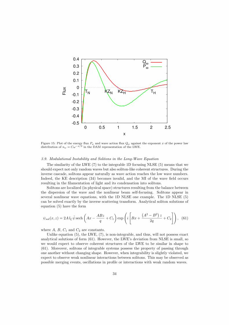
-0.5

-0.4

-0.3

-0.2

-0.1

0

0.1

0.2

0.3

0.4

0 0.5 1 1.5 2 2.5

Flu

x

x

Qω

Pω

TN THKZN KZH

Figure 15: Plot of the energy flux Pω and wave action flux Qω against the exponent x of the power lawdistribution of nω = Cω−x/2 in the DAM representation of the LWE.

3.9. Modulational Instability and Solitons in the Long-Wave Equation

The similarity of the LWE (7) to the integrable 1D focusing NLSE (5) means that weshould expect not only random waves but also soliton-like coherent structures. During theinverse cascade, solitons appear naturally as wave action reaches the low wave numbers.Indeed, the KE description (34) becomes invalid, and the MI of the wave field occursresulting in the filamentation of light and its condensation into solitons.

Solitons are localized (in physical space) structures resulting from the balance betweenthe dispersion of the wave and the nonlinear beam self-focusing. Solitons appear inseveral nonlinear wave equations, with the 1D NLSE one example. The 1D NLSE (5)can be solved exactly by the inverse scattering transform. Analytical soliton solutions ofequation (5) have the form

ψsol(x, z) = 2A lξ ψ sech

(Ax− ABz

q+ C1

)exp

(i

[Bx+

(A2 −B2

)z

2q+ C2

]), (61)

where A, B, C1 and C2 are constants.Unlike equation (5), the LWE, (7), is non-integrable, and thus, will not possess exact

analytical solutions of form (61). However, the LWE’s deviation from NLSE is small, sowe would expect to observe coherent structures of the LWE to be similar in shape to(61). Moreover, solitons of integrable systems possess the property of passing throughone another without changing shape. However, when integrability is slightly violated, weexpect to observe weak nonlinear interactions between solitons. This may be observed aspossible merging events, oscillations in profile or interactions with weak random waves.

34

Formally, 1D NLSE solitons are defined as solutions to (5) of the form [71]

ψsol(x, z) = eiΩz/2qφ

(x− V z

2q

), (62)

i.e. that the structure of the soliton is preserved as it propagates along the z-axis by somevelocity V . The Fourier transform of φ(x, z) satisfies the following integral equation:

φk = − 1

2 (Ω− kV + ωk)

∫Tk,2

3,4 φ∗2φ3φ4δ

k,23,4 dk2dk3dk4, (63)

with T 1,23,4 , in the case of the 1D NLSE, given by the first term of equation (18b), i.e.

constant. If the denominator of φk in equation (63) has no zeros for k ∈ R, then solitonsmay be present in the system. If in equation (63) the numerator and denominatorcontain only one zero each at k = 0 then solitons may also exist. For OWT, whenωk = k2, there exist soliton parameters Ω and V for which the denominator is not zero.This corresponds to the cases when on the (k, ω)-plane, the line ω = kV − Ω lies belowthe parabola ω = ωk = k2 without intersecting it. Such parameters correspond to non-radiating solitons. Let us emphasize an important difference with systems for which thereexist no straight lines on the (k, ω)-plane non-intersecting with the dispersion curve, asit is the case e.g. for the gravity waves, where ωk = k1/2, and for a the MMT modelwith the same dispersion relation [71, 91]. In the latter cases quasi-soliton structures arepossible, but they have only a finite life time because they decay via radiating weak wavesin a way similar to Cherenkov radiation [91]. In contrast, there is no radiation of wavesby solitons in our optical system, except during the soliton-soliton collisions (the latterdo create wave ripples due to the weak non-integrability of the system). In fact, we willsee that the dominant interactions are in the opposite direction: the waves “condense”into solitons with resonant parameters Ω and V i.e. such that the line ω = kV − Ωis tangentially touching the parabola ω = ωk. Subsequent evolution brings these linesfurther down thus decoupling the solitons from the weak waves. Hence, the solitons act asoptical “vacuum cleaners” which absorb “optical dirt” - the background noise consistingof weak random waves.

In figure 16, we plot the profile of the NLSE soliton (61), with the corresponding waveaction spectrum given in figure 17. We observe a scaling of nk ∝ k0 towards low wavenumbers, with a decline of the spectrum at large k. However, a nk ∝ k0 scaling is alsoobserved from the equipartition of wave action (47). Therefore, by mere observation ofthe wave action spectrum, nk, it will be difficult to determine if the wave field is comprisedof equilibrated random waves or if is in the presence of solitons. To distinguish betweenthese two states, we can numerically produce a (k, ω)-plot, that involves an additionalFourier transform over a time window. This method separates the random waves fromthe coherent component by observation of the dispersion relation, ωk [51, 47, 49].

The inverse cascade of photons is an essential step in the creation of solitons from aweakly nonlinear random wave field. The cascade provides the means, via nonlinear waveinteraction, for wave action to reach large scales. As the inverse cascade develops, thenonlinearity of the system increases and a condensate forms, resulting in the dynamicsof random waves deviating from the linear dispersion relation to one that is Bogoliubovmodified. In the LWE, this condensate is unstable, and undergoes MI resulting in theformation of solitons. To derive an expression for the Bogoliubov dispersion relation, we

35

0

500

1000

1500

2000

0 2 4 6 8 10

Inte

nsity[a

.u.]

x[mm]

Soliton

Figure 16: Intensity profile of the 1D NLSE soliton profile given in equation (61).

103

104

105

106

101

102

nk

k [mm-1

]

Soliton

Figure 17: The corresponding wave action spectrum for the soliton profile in figure 16

must first expand the wave function ψ(x, z) around a homogeneous condensate solution.The Bogoliubov dispersion relation then comprises of the wave frequency for the distur-bances upon the condensate. Its derivation can be found in Appendix G. The dispersion

36

relation is

ωBk = ωc + Ωk

= − I0

2ψ2l2ξ+

√(1 +

I0

ψ2

)k4 − I0

ψ2l2ξk2, (64)

where I0 = |ψ0|2 is the intensity of the condensate. We observe that the Bogoliubovdispersion relation (64) is the linear wave frequency ωk = k2 (when I0 = 0) with acorrection due to the formation of the condensate. Frequency (64) becomes complexwhen the term inside the square root turns negative. This gives a condition for the MI,

k2 <I0

(ψ2 + I0)l2ξ. (65)

It is MI that precedes and assists the formation of solitons when WT fails to remainweak at large scales. Note that the large scale condensate is not necessarily uniformin the physical space - it may contain a range of excited large-scale modes. However,such a condensate will be felt as quasi-uniform by modes with k significantly exceedingthe lowest wave numbers. Thus, it is best to generalize the definition of the condensateintensity. In fact, we found that the best agreement of the Bogoliubov dispersion relationto the numerical (k, ω)-plot (figure 23) was achieved when we take I0 to equal the intensityof the soliton component, i.e. the wave action contained in the region −ωmax/2 < ω < 0.Note that other classical examples of MI are also found in the context of water waves,where it is known as the Benjamin-Feir instability [131], and in the Rossby/drift waves[132].

Consideration of a single 1D NLSE soliton defined by equation (61), in an infinitelylong domain, allows for the analytical computation of the conserved quantities of the 1DNLSE system. This will provide some insight into the behavior of solitons in the LWE.Calculation of the two energy contributions in the NLSE Hamiltonian are given by

H2 =

∫ ∞−∞

∣∣∣∣∂ψsol

∂x2

∣∣∣∣2 dx =8Aψ2l2ξ

(A2 + 3B2

)3

, (66a)

H4 = − 1

4ψ2l2ξ

∫ ∞−∞|ψsol|4 dx = −

16A3ψ2l2ξ3

. (66b)

Although, exact NLSE solitons do not interact, solitons in the LWE will because ofthe additional non-integrable term. Therefore, we will most probably observe behaviorsuch as growing, shrinking, merging and collapsing. If we consider the A-dependenceof equations (66), then we observe that the nonlinear energy of the soliton increases attwice the rate (with respect to A) compared to the linear energy. However, for the systemto conserve energy, the linear and nonlinear energies must remain balanced for all time(with their sum equal to some initial energy, E0). From (66) this initial energy is givenby

Hsol = E0 =8ψ2l2ξA

(3B2 −A2

)3

. (67)

37

For the same energy, equation (67) implies the relation

B =

√E0

3A+A2

3, (68)

i.e. for the soliton to grow in amplitude A, it must also increase its speed ∼ B/q, inorder to compensate for the balance between the linear and nonlinear energies. However,this would increase the wave action N and the linear momentumM - another conservedquantity of the system. Therefore, an important question to ask is, can two solitonsmerge, while wave action, energy, and linear momentum remain conserved?

The answer to this is yes, but only if the merging of two solitons generate waves. Letus prove this fact. Consider two solitons with parameters A1, B1 and A2, B2, thatdefines their amplitude and speed respectively, and then assume that the two solitonsmerge into one soliton defined by A3, B3, see figure 18 for an illustration,

Waves

Inte

nsi

ty

x

Before Merging After Merging

Inte

nsi

ty

x

A ,B 3 3

1

A ,B 2 2

A ,B 1

Soliton2

Soliton Soliton31

Waves

Figure 18: Graphic to show the before and after states from a soliton merger. On the left image wesee two solitons with parameters A1, B1 and A2, B2, while after we see only one soliton defined byA3, B3 but with the generation of waves, with the wave energy being determined by equation (73).

The wave action N of a soliton is defined as

Nsol =

∫ ∞−∞|ψsol|2 dx = 4Aψ2l2ξ , (69)

and its momentum M is given by

Msol =i

2

∫ ∞−∞

(ψsol

∂ψ∗sol

∂x− ψ∗sol

∂ψsol

∂x

)dx = 8ABψ2l2ξ . (70)

Conservation of the total wave action and the total momentum of two solitons implythat

A3 = A1 +A2, (71a)

B3 =A1B1 +A2B2

A1 +A2, (71b)

must hold during the merging event. Now if we consider the total energy conservation,but include a term that describes the generation of energy associated to waves Hwaves (it

38

is reasonable to assume that low amplitude waves do not significantly contribute to thetotal wave action and the momentum of the system). Then the conservation of energyimplies

Hsol1 +Hsol2 = Hsol3 +Hwaves, (72)

where Hsoli is the energy defined by equation (67) of soliton i. Then using (71), (72) and(67), we have that the energy that is generated into waves is given by

Hwaves =8ψ2l2ξA1A2

[(A1 +A2)

2+ (B1 −B2)

2]

A1 +A2. (73)

Equation (73) states the amount of energy that is transferred to waves from the solitonmerging event and is solely determined by the parameters of the initial (pre-merging)solitons. Furthermore, equation (73) implies that there must be waves generated fromthe merging of two solitons. If there were no waves created from the interaction, then theonly solution to (73) would imply A1 = 0 or A2 = 0, i.e. one of the two initial solitonsis absent. Therefore, we can expect the behavior of the LWE to be as follows: As waveaction reaches the largest scale by the inverse cascade, solitons begin to emerge via MI.As these solitons evolve, they grow in size by absorbing wave action from waves and bymerging with other solitons. But by merging with other solitons, the interaction emitslow intensity random linear waves back into the system. This process proceeds untilthere is only a single soliton remaining surrounded by a field of random linear waves.

4. Numerical results and comparison with the experiment

We present the numerical results for OWT. After presenting the numerical method,we divide this Section into two main parts, firstly, we consider the system described bythe LWE in its numerical aspect and compare with the experimental results. We beginthis Subsection by considering the decaying setup with condensation at the lowest wavenumbers. Then we move on to the numerical simulations of the LWE in the forced anddissipated regime. In the final Subsection, we present the numerical results for the SWE.

4.1. The Numerical Method

For the numerical computation of the LWE and the SWE, we implement a pseudo-spectral method [133, 134], with a resolution of N = 212 Fourier modes. The schemeutilizes the fast Fourier transform to convert physical space vectors into their Fourierrepresentation, where differentiation of the wave field is transformed to algebraic multi-plication by wave number k. The linear terms are solved exactly in Fourier space and thenconverted back into physical space with the aid of integrating factors, to greatly improvethe numerical stability. Nonlinear terms are more complicated. Multiplications involvingψ(x, z), have to be performed in physical space. Moreover, multiplication produces alias-ing errors, due to the periodicity of the Fourier series expansion of the solution. Theseerrors can be removed by artificially padding the Fourier mode representation with wavenumber modes of zero amplitude at either ends of k-space. The amount of de-aliasingis subject to the degree of nonlinearity of the equation. For us, this entails that half ofthe wave number resolution for the solution needs to be zero - a quarter at each end ofk-space [134].

39

We evolve the simulations in time by using the fourth order Runge-Kutta method[134], using a time step that is small enough so that it satisfies the Courant-Friedrichs-Lewy (CFL) condition of

maxk

(∂ωk∂k

)∆t < ∆x, (74)

where ∆x = L/N is the spacing of our spatial grid and L = 32π, is the length of ourperiodic box. Numerically we compute the non-dimensionalized equation given by

i∂ψ

∂z= −∂

2ψ

∂x2+N (ψ) + i (Fk −Dk) , (75)

where N(ψ) represents the nonlinear part of our equations. Appendix H includes thederivation of the non-dimensional versions of both the LWE and SWE. The non-dimensional LWE contains an adjustable parameter α, defined in Appendix H. For thedecaying setup, we set α = 128, so that the numerical simulation is in the same regimeas the experiment. For the forced and dissipated cases, we set α = 1024, so that thelong-wave limit is better realized. Fk = F (k) is the forcing profile, where energy andwave action are injected into the system. We define this in Fourier space, over a specificrange of wave numbers. For the direct cascade simulations we use a forcing profile givenby

F directk =

A exp(iθk) if 9 ≤ k

∆k ≤ 110 otherwise,

(76)

where A is the amplitude of forcing and θk is a random variable chosen from a uniformdistribution on [−π, π) at each wave number and at each time step and ∆k = 2π/L isthe Fourier grid spacing. For the inverse cascade simulations, we apply forcing over asmall range of wave numbers situated in the high wave number region. However, we mustallow for some Fourier modes with wave numbers larger than the forcing ones, becausesome direct cascade range is necessary for the development of the inverse cascade. Ourforcing profile for the inverse cascade simulations is given by

F inversek =

A exp(iθk) if N

16 − 10 ≤ k∆k ≤

N16 + 10

0 otherwise.(77)

In all simulations, we dissipate at high wave numbers by adding a hyper-viscosity term∝ k4 ψk. We use the fourth power of k, so that the dissipation profile is not too steepfor the formation of a bottleneck, or too shallow as to prevent a large enough inertialrange developing. At low wave numbers, we use two types of dissipation profile. Firstly,we can use a hypo-viscosity term ∝ k−4 ψk. However, this type of dissipation profile inthe 3D NLSE model has led to the WT description becoming invalid and a CB regimeto develop [49]. In these situations, the CB scenario is avoided by the use of low wavenumber friction.

To summarize, our numerical dissipation profile Dk = D(k), removes wave actionand energy from the system at low and high wave numbers. For clarity, we split Dk intothe low and high wave number contributions DL

k and DHk . At high wave numbers our

hyper-viscosity profile is defined as

DHk = νhyper k4 ψk, (78a)

40

where νhyper is the coefficient for the rate of dissipation. If we apply hypo-viscosity atlow wave numbers, then DL

k is given by

DLk =

νhypo k−4 ψk if k 6= 0

ψk = 0 if k = 0,

where νhypo is the coefficient for the rate of dissipation at low wave numbers. However,in situations where we use friction, then DL

k is defined as

DLk =

νfriction ψk if 0 ≤ k ≤ 6

0 otherwise,

where νfriction is the rate of friction dissipation.

4.2. The Long-Wave Equation

4.2.1. The Decaying Inverse Cascade with Condensation

The decaying simulation leading to photon condensation was originally reported byus in [51]. Both experimental and numerical setups are configured for decaying OWT,where an initial condition is set up and allowed to develop in the absence of any forcingor artificial dissipation. We perform the numerical simulation with the same parametersas the experiment, and present results in dimensional units for comparison.

The inverse cascade spectrum is of a finite capacity type, in a sense that only a finiteamount of the cascading invariant (wave action in this case) is needed to fill the infiniteinertial range. Indeed, this is determined as the integral of the wave action spectrum nkconverges at k = 0, i.e. ∫

0

nk dk ∝∫

0

k−3/5 dk <∞. (79)

For finite capacity spectra, the turbulent systems have a long transient (on its way tothe final thermal equilibrium state) in which the scaling is of the KZ type (provided thisspectrum is realizable, i.e. local and agrees with Fjørtoft). This is because the initialcondition serves as a huge reservoir of the cascading invariant.

Experimentally, the initial condition is setup by injecting photons at small spatialscales by modulating the intensity of the input beam with a patterned intensity mask.We randomize the phases by the use of a phase modulator. This is made by creating arandom distribution of diffusing spots with the average size ' 35 µm through the SLM.This is done in order to create an initial condition close to a RPA wave field requiredby the theory. The numerical initial condition is more idealized. We restrict the initialcondition to a localized region at small scales. The initial profile is given by

ψk(0) =

A exp(iθk) if N

16 − 5 < k∆k <

N16

ψk(0) = 0 otherwise,(80)

where A = 4.608 × 103 is the amplitude of forcing and θk is a random variable chosenfrom a uniform distribution on [−π, π) at each wave number. In dimensional units, thiscorresponds to an initial condition in the region around kf ≈ 1.5×102 mm−1. Moreover,we apply a Gaussian filter in physical space to achieve a beam profile comparable to thatof the experiment.

41

Applicability of the WT approach is verified by the calculation of the nonlinear pa-rameter LJ , equation (10), for the numerical simulation, which agrees with the exper-iment and is of the order LJ ' 100. Experimentally, we measure the light intensityI(x, z) = |ψ|2 and not the phases of ψ. Therefore the wave action spectrum nk is not di-rectly accessible. Instead, we measure the intensity spectrum, N(k, z) = |Ik(z)|2, wherethe k-scaling for Nk in the inverse cascade state is easily obtained from the KZ solu-tion (51b) and the random phase condition, (see Appendix I). This procedure gives anintensity spectrum of

Nk ∝ k−1/5. (81)

The wave action spectrum from the numerical simulation is shown in figure 19 attwo different distances, we observe at z = 0 mm the peak from the initial conditionat high wave numbers, then at z = 63 mm we observe evidence of an inverse cascade,as the majority of the wave action is situated towards low wave numbers. However, atlow wave numbers we do not see the spectrum matching our theoretical KZ prediction(51b). We showed in Section 3.8, that the wave action flux, Qk, corresponding to theKZ solution (51b), has the incorrect sign for an inverse cascade. Therefore, we notedthat the inverse cascade spectrum would correspond to a mixed thermal solution witha finite flux contribution. This is the probable cause for the lack of agreement with theKZ solution. We observe from figure 19, that nk ∝ k0 at low wave numbers, which mayaccount for the mixed thermal solution (as this scaling corresponds to the equipartitionof wave action (47b)) or for the presence of solitons (c.f. figure 17).

10-3

10-2

10-1

100

101

102

k [mm-1

]

k-3/5

z = 0 mm

z = 63 mm

nk

Figure 19: Numerical spectrum of the wave action, nk, at distances z = 0 mm and z = 63 mm.

The numerical spectrum of the light intensity is shown in figure 20. In this plot, weobserve an inverse cascade, resulting in a good agreement with the WT prediction forthe intensity spectrum (81). This agreement may be coincidental, as we have shown thatthe flux directions are insufficient for a KZ wave action cascade. However, the intensity

42

spectrum is a non-local quantity, and the system may, somehow, conspire to have betterscaling properties of the KZ type for the intensity than for the wave action density. Wecan only confidently say that we still do not fully understand the agreement.

Verification of the long-wave limit klξ 1 and deviation from integrability is checkedby considering the ratio of the two nonlinear terms in the LWE (7), which we denoteas R, and is estimated in Fourier space as R ∝ k2l2ξ . We observe from the experimentand the numerical simulations, respectively, figures 7 and 20, that the inverse cascade isapproximately in the region k ∼ 104 − 105 m−1, giving an estimation of R ∼ 10−2 − 1.Note, that if R is too small, then we are close to an integrable system, which would bedominated by solitons and lack cascade dynamics, and if R is too high then the LWE isa poor approximation for 1D OWT.

10-1

100

101

102

|Ik|2

k [mm-1

]

k-1/5

z = 0 mm

z = 63 mm

Figure 20: Numerical spectrum of the light intensity, Nk = |Ik|2 at two different distances z. Averagingis done over a small finite time window and over ten realisations.

The numerical simulation of the intensity distribution I(x, z), showing the beamevolution during propagation is displayed in figure 21. Both the experimental and thenumerical results, respectively figures 8 and 21, indicate that the total number of soli-tons reduces. The observed increase of the scale and formation of coherent structuresrepresents the condensation of light. Experimentally, the condensation into one domi-nant soliton is well revealed by the intensity profiles I(x) taken at different propagationdistances, as shown in figure 9 for z = 0.3, 4.5 and 7.5 mm. Note that the amplitude ofthe final dominant soliton is three orders of magnitude larger than the amplitude of theinitial periodic modulation.

4.2.2. The PDF of the light intensity

Numerically, we have computed the PDF of the light intensity and, for comparisonwith the experiment, we plot in figure 22 three PDFs at distances z = 0 mm, z = 31

43

Figure 21: Numerical results for intensity distribution I(x, z). The frame on the left is a magnifiedsection of the initial propagation of the beam.

mm and z = 63 mm. As in the experiment (see figure 11) we observe deviations froma pure Gaussian field, with a slower that exponential decay of the PDF tails. Again,non-Gaussianity corresponds here to intermittency of WT and, indeed, it accompaniesthe development of coherent structures (solitons) in the system.

4.2.3. The k − ω Plots: Solitons and Waves

To allow us to capture the inverse cascade dynamics in more detail and to enable usto visualize solitons and analyze their interactions with incoherent waves, we perform anadditional decaying simulation with a lower initial intensity. However, to compensate forthe lower intensity initial condition, we must run the simulation for much longer times.Separation of the random wave and the coherent soliton components can be achievedby performing an additional Fourier transform with respect to z over a finite z-windowwhich results in the 2D Fourier (k, ω)-plots of wave action density [47, 51].

The numerically obtained (k, ω)-plot enables the direct observation of the dispersionrelation of random waves, and is shown in figure 23. Here, the incoherent wave compo-nent is distributed around the wave dispersion relation, which is Bogoliubov-modified bythe condensate, (64), and is shown by the solid line in figure 23. The distribution of thedispersion relation is centered around the theoretical prediction (64). We observe thatthe width of the dispersion relation is narrow for large k, a sign of weak nonlinearity,and progressively gets wider as it approaches smaller wave numbers. This broadening,is an indication that the nonlinearity of the system increases towards smaller k, as wastheoretically predicted in Section 3.7. At wave numbers around zero, we see that the the-oretical Bogoliubov curve vanishes, corresponding to the region defined by equation (65),where the frequency becomes complex. For such wave numbers k, MI of the wave packetsoccurs and the WT description breaks down. Below the region where the Bogoliubov

44

10-3

10-2

10-1

100

0 2 4 6 8 10 12

PD

F(I

/<I>

)

I/<I>

0 mm31 mm63 mm

exp(-I/<I>)

Figure 22: Normalized PDFs of the wave intensity within the numerical cell at three different distancesalong the cell, z = 0 mm, 31 mm and z = 63 mm. The black dashed straight line corresponds to theRayleigh PDF corresponding to a Gaussian wave field.

Figure 23: The (k, ω)-plot of the wave field at z = 10 m. The Bogoliubov dispersion relation is shownby the dashed green line.

relation becomes complex, we observe slanted lines. Each of these lines corresponds toa coherent soliton, whose speed is equal to the slope of the line. To examine the time

45

evolution of the system, we have put together successive (k, ω)-plots into a movie. Weobserve that the formation of solitons is seen in the movie as straight lines peeling with agradient tangential to the dispersion curve. Moreover, we observe the gradual migrationof these lines to higher negative frequencies, as the solitons begin to grow in size by theabsorption of energy from surrounding waves or by merging with other solitons.

Further analysis can be done by separating the wave and the soliton components ofthe (k, ω)-plot. We define the soliton region of the (k, ω)-plot as the region defined with−ωmax/2 < ω < 0, (where ωk ranges from [−ωmax, ωmax) and ωmax = k2

max in the (k, ω)-plot). We chose this region to represent the soliton component because we found thatsome wave component of the dispersion relation appears in the extreme negative ω-regiondue to the periodicity of the Fourier transform and possibly from an insufficient timewindow for the Fourier transform in z. Consequently, the wave component is definedas the region of the (k, ω)-plot outside the soliton region. By inverting the Fouriertransforms of each of the soliton and wave regions separately, we can recover the wavefield ψ(x, z) for each component. This enables us to compare the soliton and wavecomponents of the intensity profile, figure 24, and the wave action spectrum, figure 25.In figure 24, we plot the intensity profile of light in real space for the soliton and wavecomponents. We see that our procedure does indeed isolate the coherent solitons fromthe random wave background and we observe that the main soliton is a least an order ofmagnitude greater than the random wave field.

0

500

1000

1500

2000

0 2 4 6 8 10

Inte

nsity[a

.u.]

x[mm]

Wave

Soliton

Figure 24: Plot of the intensity profile at z = 10 m of both the soliton and wave components

In figure 25, we observe that the soliton component of the wave action spectrum,is situated towards the low wave number region and scales as ∝ k0. This profile isqualitatively similar to the wave action spectrum of the exact soliton of the 1D NLSE,seen in figure 16. The wave component of the wave action spectrum is more widelydistributed in k-space. Taking into account that the initial spectrum was concentrated

46

near k = 1.5 × 102mm−1, we see that, roughly, the inverse cascade range is solitondominated and the direct cascade range is random-wave dominated in this run. Wealso put a slope corresponding to the inverse cascade KZ spectrum to show that itstrongly disagrees with the spectrum in the soliton dominated range. In the directcascade range, the spectrum is consistent with the thermalized spectrum for energy(47a). For comparison, we also plot the direct cascade KZ scaling in figure 25. We seethat the thermalized spectrum is in a much better agreement with the data than KZ .This is not surprising, as the decaying simulation is void of any dissipation mechanism,so energy would tend to thermalize. We would expect to see a better test of the KZpredictions in the forced and dissipated simulations where a non-equilibrium stationarystate can be achieved.

Note that in other wave systems, the separation of the coherent and wave components,may be a useful technique in observing the KZ scaling otherwise masked by the presenceof coherent structures.

10-1

100

101

102

103

100

101

102

nk [

a.u

.]

k [mm-1

]

Total

Wave

Soliton

k-3/5

k-1

ln(kl)-1/5

k-2

InitialCondition

Figure 25: The wave action spectrum of both the soliton and wave components of the spectrum, withthe KZ and thermalized energy predictions for comparison.

From the same simulation, we plot the (x, z)-plot for the intensity distribution, I(x, z),in figure 26. With the longer propagation distance, we observe the formation and evolu-tion of solitons from the weakly nonlinear background. In the initial stages of the sim-ulation, we observe enlargement of the characteristic wavelength of the random wavesfollowed by the formation of numerous solitons out of the random wave background. Asthe simulation progresses, the solitons become more pronounced and begin to behaveindependently from the waves, with an almost random movement through the numericalbox. A large number of solitons are produced at the beginning of the simulation, butover long evolution times, the number of solitons reduces, with the remaining solitonsbeing of increasing amplitude. Indeed, there are many soliton merging events. In fig-

47

ure 27b we see a magnified section of a merging event from figure 26. At late times,figure 26 shows a single dominant soliton in the system that has subsequently grown byabsorption of energy from fellow solitons and the background wave field. Such a finalsingle-soliton state is also observed in the experiment (figure 8), albeit at a much shorterpropagation distance, with the multi-soliton range missing. In the future, it would beinteresting to set-up a larger experiment which could capture the multi-soliton transientstate. In figure 27, we plot three zoomed sections of figure 8 to highlight aspects of thesoliton behavior. In figure 27a, we observe several solitons passing through one anotherwith little deviation in their trajectories. Moreover, the weaker solitons (light gray incolor), have almost straight trajectories, like freely propagating linear waves, whilst thestronger solitons’ movements are more erratic.

In figure 27b, we magnify a merging event between two solitons. The larger solitonengulfs the smaller soliton almost without any deviation in its trajectory. Therefore, inthe numerical simulation, large solitons absorb energy from smaller solitons, reducing thetotal number within the system. In addition, we also observe at z = 11.5 m, a solitonbouncing off the larger soliton. As the weaker soliton approaches the larger soliton, itslows, before moving away at a fast speed. When two solitons merge and when theyrepel is a key question that still remains to be answered. Finally, in figure 27c, weobserve two weak solitons propagating together, until around z = 13 m, when they bothrepel each other and disperse back into the random wave field. This shows the breakup of the coherent structures and the subsequent re-injection of wave action into highfrequency waves. All these events are parts of the WTLC, i.e. the cycle of coexistenceand interactions of the random waves and the solitons and their mutual transformationsinto one another.

In figures 28 and 29, we plot the maximum of the intensity and the energy of thesystem with z. To begin, we note that the maximum of the intensity of the wave field isalways growing, and moreover, we observe that there is a sharp increase in the maximumat around z = 11 m. This jump corresponds to the merging event seen in figure 27b.Thus, the dominant soliton instantly grows in size once it absorbs the other soliton. Thismerging event is also noticed in figure 29, where we observe a similar sharp increase tothe linear and nonlinear energies at z = 11 m, showing that as the dominant soliton’samplitude increases, there is a significant increase in the nonlinearity of the system. Itis interesting that the amplitude of the final dominant soliton continues to grow at thelate stages of this simulation, e.g. in the range of z between 15 m and 20 m. Thissoliton acts as a kind of “optical vacuum cleaner” which, as it moves, sucks in energy ofthe random waves and remaining soliton debris (i.e. soliton-like structures which are soweak that they cannot maintain their coherence for long).

From the beginning, the nonlinear energy, associated mostly with the first nonlinearterm in the evolution equation (7), grows almost by an order of magnitude in size,compared to just under double in size for the linear contribution. This indicates that theinverse cascade and the subsequent soliton development is associated with an increasein the nonlinearity of the system, and hence the breakdown of the WT description.Moreover, we note that the total energy remains conserved, verifying that our simulationis well-resolved.

In figures 30, we present the soliton and wave components of the energies evolvingwith z. The data was made by using the same soliton-wave separation technique as theone we described previously, now using a series of (k, ω)-plots and computing the energy

48

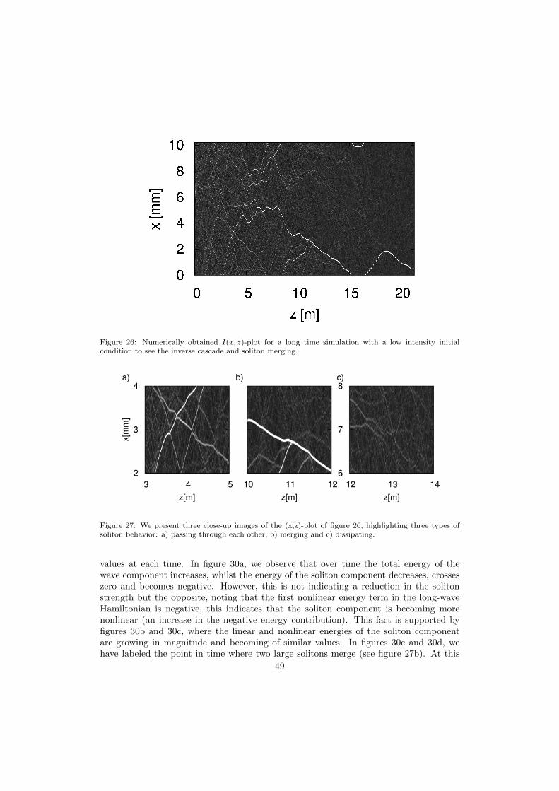
Figure 26: Numerically obtained I(x, z)-plot for a long time simulation with a low intensity initialcondition to see the inverse cascade and soliton merging.

Figure 27: We present three close-up images of the (x,z)-plot of figure 26, highlighting three types ofsoliton behavior: a) passing through each other, b) merging and c) dissipating.

values at each time. In figure 30a, we observe that over time the total energy of thewave component increases, whilst the energy of the soliton component decreases, crosseszero and becomes negative. However, this is not indicating a reduction in the solitonstrength but the opposite, noting that the first nonlinear energy term in the long-waveHamiltonian is negative, this indicates that the soliton component is becoming morenonlinear (an increase in the negative energy contribution). This fact is supported byfigures 30b and 30c, where the linear and nonlinear energies of the soliton componentare growing in magnitude and becoming of similar values. In figures 30c and 30d, wehave labeled the point in time where two large solitons merge (see figure 27b). At this

49

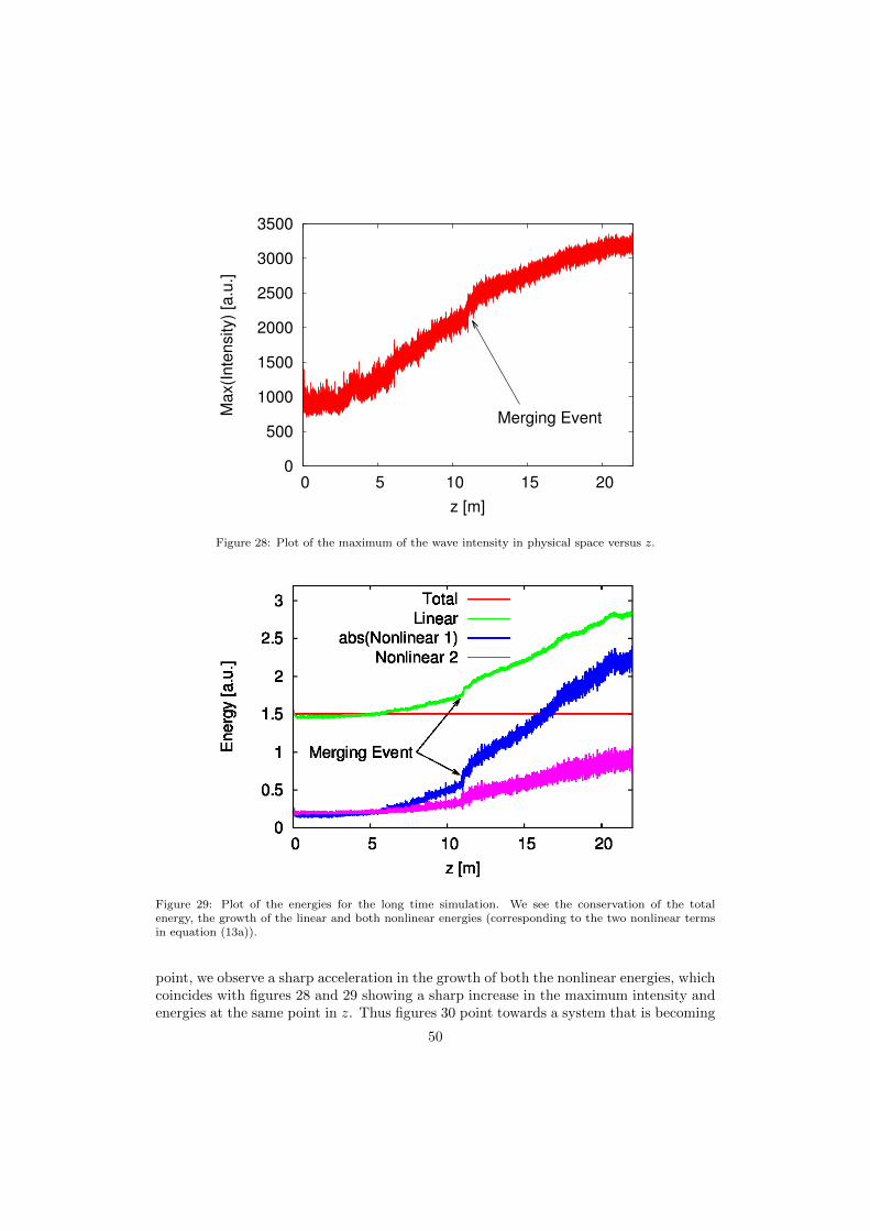
0

500

1000

1500

2000

2500

3000

3500

0 5 10 15 20

Ma

x(I

nte

nsity)

[a.u

.]

z [m]

Merging Event

Figure 28: Plot of the maximum of the wave intensity in physical space versus z.

Figure 29: Plot of the energies for the long time simulation. We see the conservation of the totalenergy, the growth of the linear and both nonlinear energies (corresponding to the two nonlinear termsin equation (13a)).

point, we observe a sharp acceleration in the growth of both the nonlinear energies, whichcoincides with figures 28 and 29 showing a sharp increase in the maximum intensity andenergies at the same point in z. Thus figures 30 point towards a system that is becoming

50

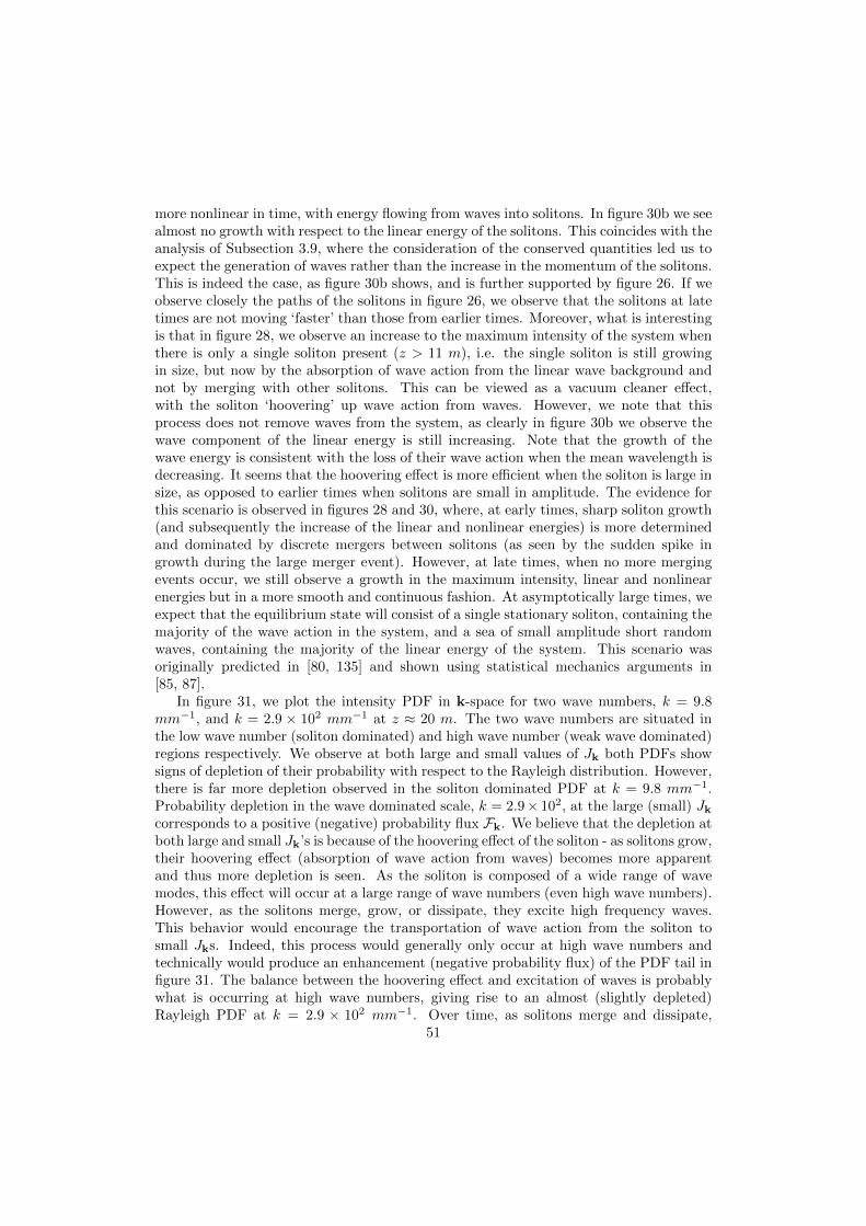
more nonlinear in time, with energy flowing from waves into solitons. In figure 30b we seealmost no growth with respect to the linear energy of the solitons. This coincides with theanalysis of Subsection 3.9, where the consideration of the conserved quantities led us toexpect the generation of waves rather than the increase in the momentum of the solitons.This is indeed the case, as figure 30b shows, and is further supported by figure 26. If weobserve closely the paths of the solitons in figure 26, we observe that the solitons at latetimes are not moving ‘faster’ than those from earlier times. Moreover, what is interestingis that in figure 28, we observe an increase to the maximum intensity of the system whenthere is only a single soliton present (z > 11 m), i.e. the single soliton is still growingin size, but now by the absorption of wave action from the linear wave background andnot by merging with other solitons. This can be viewed as a vacuum cleaner effect,with the soliton ‘hoovering’ up wave action from waves. However, we note that thisprocess does not remove waves from the system, as clearly in figure 30b we observe thewave component of the linear energy is still increasing. Note that the growth of thewave energy is consistent with the loss of their wave action when the mean wavelength isdecreasing. It seems that the hoovering effect is more efficient when the soliton is large insize, as opposed to earlier times when solitons are small in amplitude. The evidence forthis scenario is observed in figures 28 and 30, where, at early times, sharp soliton growth(and subsequently the increase of the linear and nonlinear energies) is more determinedand dominated by discrete mergers between solitons (as seen by the sudden spike ingrowth during the large merger event). However, at late times, when no more mergingevents occur, we still observe a growth in the maximum intensity, linear and nonlinearenergies but in a more smooth and continuous fashion. At asymptotically large times, weexpect that the equilibrium state will consist of a single stationary soliton, containing themajority of the wave action in the system, and a sea of small amplitude short randomwaves, containing the majority of the linear energy of the system. This scenario wasoriginally predicted in [80, 135] and shown using statistical mechanics arguments in[85, 87].

In figure 31, we plot the intensity PDF in k-space for two wave numbers, k = 9.8mm−1, and k = 2.9 × 102 mm−1 at z ≈ 20 m. The two wave numbers are situated inthe low wave number (soliton dominated) and high wave number (weak wave dominated)regions respectively. We observe at both large and small values of Jk both PDFs showsigns of depletion of their probability with respect to the Rayleigh distribution. However,there is far more depletion observed in the soliton dominated PDF at k = 9.8 mm−1.Probability depletion in the wave dominated scale, k = 2.9× 102, at the large (small) Jkcorresponds to a positive (negative) probability flux Fk. We believe that the depletion atboth large and small Jk’s is because of the hoovering effect of the soliton - as solitons grow,their hoovering effect (absorption of wave action from waves) becomes more apparentand thus more depletion is seen. As the soliton is composed of a wide range of wavemodes, this effect will occur at a large range of wave numbers (even high wave numbers).However, as the solitons merge, grow, or dissipate, they excite high frequency waves.This behavior would encourage the transportation of wave action from the soliton tosmall Jks. Indeed, this process would generally only occur at high wave numbers andtechnically would produce an enhancement (negative probability flux) of the PDF tail infigure 31. The balance between the hoovering effect and excitation of waves is probablywhat is occurring at high wave numbers, giving rise to an almost (slightly depleted)Rayleigh PDF at k = 2.9 × 102 mm−1. Over time, as solitons merge and dissipate,

51

-1

-0.5

0

0.5

1

1.5

2

2.5

3

2 4 6 8 10 12 14 16 18 20

To

tal E

ne

rgy[a

.u.]

z[m]

Merging Event

SolitonWave

(a) Evolution of the total energy.

0

0.5

1

1.5

2

2.5

3

2 4 6 8 10 12 14 16 18 20

Lin

ea

r E

ne

rgy[a

.u.]

z[m]

Merging Event

SolitonWave

(b) Evolution of the linear energy.

-1.4

-1.2

-1

-0.8

-0.6

-0.4

-0.2

0

2 4 6 8 10 12 14 16 18 20

No

nlin

ea

r E

ne

rgy 1

[a.u

.]

z[m]

Merging Event

SolitonWave

(c) Evolution of the first nonlinear energy term.

0.05

0.1

0.15

0.2

0.25

0.3

0.35

0.4

0.45

0.5

2 4 6 8 10 12 14 16 18 20

No

nlin

ea

r E

ne

rgy 2

[a.u

.]

z[m]

Merging Event

SolitonWave

(d) Evolution of the second nonlinear energy term.

Figure 30: Plot of the evolution of the (a) total energy, (b) linear energy, (c) first nonlinear energy term,and (d) second nonlinear energy term, of the soliton and wave components versus z.

until only one remain, we would observe a reduction in the re-injection of wave action athigh wave numbers because the mechanisms that allow this (merging and dissipation ofsolitons) would cease. At low wave numbers, at k = 9.8 mm−1, the PDF would graduallybecome more and more depleted (deviated from Rayleigh) as time progresses. As thisscale is soliton dominated, we cannot apply our theory of the PDF depletion in termsof the probability flux Fk which was developed for weak waves. In fact, such a PDFcorresponds to a certain distribution of solitons in the soliton parameter space (A,B) forwhich a theory has not yet been developed.

The observed directions of the probability flux directions Fk - toward large Jks at lowwave numbers and to low Jks at high wave numbers - can be combined with the pictureof the inverse cascade energy flux in the direction of low wave numbers by consideringa 2D flux pattern on the (k, Jk)-plane. This yields a diagram for the WTLC presentedin figure 32. Here, the initial condition is at high wave numbers and low Jks (weaksmall-scale random waves). The inverse cascade transports wave action, via six-wavemixing, to small wave numbers and to higher Jks, as the inverse cascade is associatedwith an increase in nonlinearity of the system. As wave action accumulates at large scales,MI kicks in and solitons form, with wave action spreading along the soliton spectrum

52

nk ∝ k0. Note that the wave modes within the soliton are coherent, i.e. correlatedwith each other. The non-integrability of the system allows for solitons to interactwith surrounding structures, that enable energy exchange. In particular, solitons willcollide, occasionally merge or deteriorate via random interactions - each of these processesallowing for the emission of energy and wave action to incoherent waves, resulting in areversal of the probability flux F at high wave numbers. The wave action re-injectedback into the random wave component fuels the continual process of the inverse cascade.This continuous transport of wave action can be seen as a vortex-like flux structure in the(k, Jk)-plane which we call the WTLC in our 1D OWT system [11, 56]. Note that fromfigure 31 we see a positive probability flux even at high wave numbers! Thus, the WTLCpicture with flux lines not emerging and not terminating anywhere, as in figure 32, is onlyvalid for a steady state, whereas figure 31 corresponds to an evolving transient wherethe net flux (produced by the hoovering effect) is still directed from waves to (growing)solitons. For the LWE, the asymptotical final state is a single soliton containing most ofwave action and surrounded by almost linear waves containing finite energy but almostno wave action.

10-3

10-2

10-1

100

0 1 2 3 4 5

PD

F(s

k/<

sk>

)

sk/<sk>

k = 9.8 [mm-1

]

k = 2.9 × 102 [mm

-1]

exp(-sk/<sk>)

sk-10

10-2

100

100

101

Figure 31: PDF of intensity Jk, P = 〈δ(sk−Jk)〉, at two wave numbers, k = 9.8 mm−1, and k = 2.9×102

mm−1. The black dashed line is the Rayleigh distribution that corresponds to a Gaussian wave field.The inset shows the power-law behavior of the PDF tails. The black dashed line in the inset is s−10

k .

4.2.4. Forced and Dissipated Simulations

In this Subsection, we explore numerical simulations of the LWE and SWE withforcing and dissipation. This setup is intended to produce more idealized conditions fornon-equilibrium stationary states assumed for the realizability of pure the KZ solutions,(51). Thus, we can test to see if the KZ spectra are realizable in principle, or if theycan not be established at all, even in the most idealized of settings. In an infinite

53

Figure 32: Diagram of the WTLC. The high wave number initial condition subsequently gets transferredto low k and high Jk by the inverse cascade. At low k, the weak WT fails (near the T -junction of thedashed lines) and MI occurs, solitons form resulting in the wave action getting spread along a nk ∝ k0

spectrum (horizontal dashed line). The emission of waves from merging or deteriorating solitons re-injects wave action at low intensities.

sized system, both the direct- and the inverse-cascade ranges can be realized in the samesimulation, with forcing acting at an intermediate scale and two inertial ranges either side(see figure 14). However, computational restrictions make it impractical to perform sucha simulation. Therefore, we simulate each cascade separately, by performing a simulationfor each with forcing at either ends of k-space, allowing for just one inertial range. Wenumerically solve the non-dimensionalized equation (see Appendix H) with α = 1024.We run the simulations with a time step of ∆t = 1 × 10−4 in a box of length L = 32π,with spatial resolution of N = 212. The simulations are run so that a non-equilibriumsteady state is achieved. This is checked by observing stationarity of the total energy Hand wave action N in the system.

For the direct cascade setup for the LWE, we introduce dissipation profiles at the twolimits of k-space that removing energy and wave action that is being constantly injectedby the forcing. We set the low wave number dissipation profile, DL

k , to be friction, definedby (78b), with the friction coefficient of νfriction = 5× 10−1 and apply a hyper-viscositydissipation scheme at high wave numbers with a coefficient of νhyper = 1×10−13. Forcingis situated at large scales and is defined by (76), with amplitude A = 4.1×104. Once thesimulation has reached a statistically non-equilibrium statistical steady state, we analyzethe statistics by performing time averages over this steady state regime. We have plottedthe wave action spectrum nk for the direct cascade regime in figure 33.

We observe that the wave action spectrum in figure 33 does not agree with thetheoretical KZ prediction (55). There is a clear flat spectrum of the form nk ∝ k0. Thiscould correspond to several phenomena: solitons, critical balance and a thermalized statewith equipartition of wave action. However, in figure 34, we have plotted the (k, ω)-plotfor the same simulation at late times. We observe an absence of any soliton structures,

54

105

106

107

10-1

100

101

nk

k

nk

k-1

log(kl)-1/5

k0

Forcing

Figure 33: The wave action spectrum nk in a statistically non-equilibrium stationary state for the directcascade simulation of the LWE. We plot two black lines to show the theoretical comparisons. The blackdashed line represent the WT prediction of the KZ solution nk ∝ k−1 ln(k`). The black dotted linerepresents the thermalization of wave action.

like the ones we saw in the decaying case (see figure 23). Therefore, we can safely reasonthat the flat spectrum is not associated with the presence of solitons within the system.The explanation for the k0 slope is more likely down to the thermalization of the systemwith respect to wave action around the low to the intermediate wave number range.This behavior should be expected due to the lack of agreeing flux signs with Fjørtoft’sargument for the LWE, where a system in such a situation would tend towards a modifiedthermalization spectrum [50] also known as a “warm cascade” [49]. The lack of agreementwith the KZ spectrum can be explained by the incorrect flux directions which can bemost easily understood and determined using the DAM in Subsection 3.8. It remains tobe understood why we observe that the wave action spectrum corresponds more closelywith the thermalized KE solution corresponding to the equipartition of wave action, andnot the thermalized spectrum corresponding to the equipartition of energy. On the otherhand, we observe that the (k, ω)-distribution is not too narrow around the dispersioncurve ω = ωk = k2. Thus, we cannot rule out that the CB mechanism could be the realreason for the flat spectrum.

In figures 35 we plot PDFs of (a) the wave intensity in the physical space and (b)the Fourier-mode intensity at two different wave numbers. In figure 35a, we observe analmost perfect agreement of the the PDF to the Rayleigh distribution. This indicatesthat the system corresponds to a Gaussian wave field - a good indication that the systemis in a thermalized state of random waves. Additionally in figure 35b we observe thatboth PDFs are Rayleigh distributed (here the Rayleigh distribution is fitted to the tailsof the PDFs). Again, we observe a clear agreement of the tails to the straight line of theRayleigh distribution at large amplitudes. Towards the core of the PDFs in figure 35b we

55

Figure 34: (k, ω)-plot for the direct cascade simulation of the LWE. The green line represents the linearwave frequency ωk = k2.

see some depletion of the PDFs to the Rayleigh distribution the origin of which remainsunclear. It is possible that this is a signature of appearance of an embryonic condensate(the true condensate, solitons, are are not present in this system due to low wave numberdissipation) - a similar effect was observed in recent simulations of the 3D NLSE [49].

10-4

10-3

10-2

10-1

100

0 2 4 6 8 10

PD

F(I

/<I>

)

I/<I>

PDF(I/<I>)exp(-I/<I>)

(a)

10-2

10-1

100

0 1 2 3 4 5

PD

F(s

k / <

sk>

)

sk / <sk>

k = 2

k = 10

Rayleigh

(b)

Figure 35: (a) Normalized PDF of the wave intensity in the direct cascade simulation of the LWE. Thestraight line corresponds to the Rayleigh distribution. (b) Normalized PDF of Jk at two wave numbersfor the direct cascade in the LWE. The black dashed line represents the Rayleigh distribution.

The inverse cascade displays more unusual behavior. The inverse cascade simulationfor the LWE was setup with forcing situated at high wave numbers with a profile given byequation (77) and with low wave number dissipation in terms of friction and high wave

56

number dissipation in terms of hyper-viscosity. The parameters used for the simulationare A = 7.7× 103 for the forcing amplitude, νfriction = 1× 10−1 and νhyper = 1× 10−11

for the dissipation coefficients. As usual, we wait for a non-equilibrium stationary stateto be achieved before performing any analysis.

105

106

107

10-1

100

101

nk

k

nk

k-3/5

Forcing

Figure 36: The wave action spectrum, nk, in a statistically non-equilibrium stationary state for theinverse cascade simulation of the LWE. The straight line represents the WT prediction of the KZsolution of nk ∝ k−3/5.

In figure 36 we plot the wave action spectrum from the numerical simulation, timeaveraged once the simulation has reached a non-equilibrium stationary state. For com-parison, we also show the KZ prediction for the inverse cascade of wave action. Weobserve a lack of agreement to any power-law behavior to the spectrum. Indeed, wesee a peak of the spectrum around the forcing region, while the spectrum gradually falloff at small and large k. The absence of a KZ spectrum can be explained by the in-correct flux directions, but what is really surprising is the omission of any thermalizedor CB spectrum. The CB in this case, is identical to the spectrum of the spectrum ofthe thermalization of wave action: nk ∝ k0. CB has been observed in other opticalsystems, i.e. one described by the 3D NLSE [49]. We found that the spectrum to theleft of the forcing region seemed to be determined by the level of friction used at lowwave numbers. By tuning the coefficient of friction, we adjusted the asymptotic value ofthe spectrum at k = 0, and the spectrum would simply gradually decline to that levelfrom the forcing region. Dampening of these low wave number modes could preventsome non-local behavior that is driving the inverse cascade. Clearly, the dampening ofthese modes is restricting MI and the formation of solitons, which may have an essentialrole in the dynamics of the inverse cascade - as we do not observe this behavior in thedecaying simulation of the previous Subsection. To be certain that we are not observingany effects that might be attributed to the presence of solitons, we show the (k, ω)-plotfor the simulation in figure 37. In figure 37 we observe that no solitons are present by

57

the lack of any coherent straight lines around dispersion curve. However, if one looksclosely, we do observe the partial formation of a soliton situated on the dispersion curveat k = 15. However, with the presence of dissipation this soliton does not ‘peel’ fromthe wave component. Moreover, inspection of the intensity distribution (not shown),does not provide any indication of coherent soliton like structures distinguishable fromrandom waves. The (k, ω)-plot is also in good agreement to the linear dispersion relationωk = k2 shown by the green dashed curve, but the width of the plot is as wide as ωk inthe inverse cascade range. This implies that the system is indeed in a strongly nonlinearregime which could point at CB but, as we have already mentioned, the CB spectrum isnot observed. We have also done simulations with weaker forcing amplitudes for whichWT was weak, and the result was similar to the one reported here. In fact, the reasonthat we increased the forcing was an attempt to strengthen the wave interactions in orderto “push” the inverse cascade through to the large scales.

Figure 37: (k, ω)-plot for the inverse cascade simulation of the LWE. The green line represents the linearwave frequency ωk = k2.

In figures 38 we plot PDFs of (a) the wave intensity in the physical space and (b) of theFourier-mode intensity at two different wave numbers. Similarly to the direct cascade, weobserve agreement to the Rayleigh distribution of a Gaussian wave field. The PDF of thewave intensity in figure 38a is in perfect agreement to the unfitted Rayleigh distribution,whilst we observe good Rayleigh agreement of the tails of the PDFs in figure 38b at twowave number either end of the inertial range. Moreover, we observe a depletion of theprobability at low wave mode intensities at both k = 2 and k = 10, the same phenomenonas seen in the direct cascade.

In the simulation of the forced-dissipated inverse cascade, we see no agreement ofthe KZ, thermal or CB spectra. Moreover, we observe that the spectrum seems to bedetermined by the value of the lowest mode. This suggests that the inverse cascade maybe associated to some non-local effect established by MI. Indeed, we find the forced-dissipated simulation to provide more questions than answers to the behavior of 1D

58

10-4

10-3

10-2

10-1

100

0 2 4 6 8 10

PD

F(I

/<I>

)

I/<I>

PDF(I/<I>)exp(-I/<I>)

(a)

10-2

10-1

100

0 1 2 3 4 5

PD

F(s

k / <

sk>

)

sk / <sk>

k = 2

k = 10

Rayleigh

(b)

Figure 38: (a) Normalized PDF of the wave intensity in the inverse cascade simulation of the LWE. Thestraight line corresponds to the Rayleigh distribution. (b) Normalized PDF of Jk at two wave numbersfor the inverse cascade in the LWE. The black dashed line represents the fitted Rayleigh distribution.

OWT, and clearly more work in this area is needed to fully explain these results.

4.3. The Short-Wave Equation

We investigate the SWE, (9) by numerical simulations of the non-dimensionalizedmodel of Appendix H. We apply the same forcing and dissipation profiles that are de-scribed in Section 4.1. We dissipate at low wave numbers using a hypo-viscosity profile,while using hyper-viscosity at high wave numbers.

We begin by discussing the direct cascade simulation. We force the system with theprofile (76), with amplitudeA = 1.6×102 and use the dissipation rates of νhypo = 1×10−2,νhyper = 1× 10−11 for the direct simulation.

In figure 39 we plot the wave action spectrum for the direct cascade averaged overa time window once the system has reached a statistically non-equilibrium steady state.We observe a good agreement to the WT prediction (52a). However, notice that there issome slight deviation of the spectrum in the middle of the inertial range. This is likely tobe caused by an insufficient time average of the statistics. The agreement is surprising,as we showed that the KZ solution, (52a), does not produce convergence of the collisionintegral in the UV limit. However, we may be observing a non-local spectrum that isclose to the local WT prediction.

In figures 40 we plot the normalized PDF for the wave intensity in physical space andin Fourier space respectively. We observe in figure 40a that there is a slight deviationto the Rayleigh distribution (corresponding to a Gaussian wave field) at high intensities.This implies that there is a larger than expected occurrence of high intensity structures- a sign of wave intermittency. The SWE does not seem to produce solitons, but wecan numerically check this fact my investigating the (k, ω)-plot in figure 41. WT theoryimplies that such behavior should exist as part of a wave breaking process. In addition,in figure 40a we see a large accumulation of the probability at low intensities, far morethan what is predicted by the Rayleigh distribution indicating an enhanced presence ofdark regions void of light. On the other hand, figure 40b is the PDF of Jk at two wavenumbers at either end of the inertial range. We see that the PDF at k = 1 remains

59

100

102

104

10-1

100

101

nk

k

nk

k7/5

Forcing

Figure 39: The wave action spectrum nk in a statistically non-equilibrium stationary state for the directcascade simulation of the SWE. The straight line represents the WT prediction of the KZ solution ofnk ∝ k7/5.

10-4

10-3

10-2

10-1

100

0 2 4 6 8 10 12

PD

F(I

/<I>

)

I/<I>

PDF(I/<I>)Rayleigh

(a)

10-2

10-1

100

0 1 2 3 4 5 6 7 8

PD

F(s

k / <

sk>

)

sk / <sk>

k = 1

k = 7

exp(-sk/<sk>)

(b)

Figure 40: (a) Normalized PDF of the wave intensity in the direct cascade simulation of the SWE. Thestraight line corresponds to the fitted Rayleigh distribution. (b) Normalized PDF of Jk at two wavenumbers for the direct cascade in the SWE. The black dashed line represents the Rayleigh distribution.

relatively close to the Rayleigh distribution, with only a minor depletion in the tail.At k = 7 we observe a large enhancement of the PDF at large Jk, corresponding to anegative probability flux Fk. Therefore, we see behavior that is similar to that whichis described by the WTLC, figure 32. Observation of the (k, ω)-plot, figure 41, showsthat actually there are no coherent structures present in the system. This conclusion ismade by the lack structures at negative ω. Moreover, we see a clear accumulation of thedispersion curve situated around the linear wave frequency ωk = k2. This indicates thatthe system is in the weak nonlinear limit.

60

Figure 41: (k, ω)-plot for the direct cascade simulation of the SWE. The dashed green line representsthe linear wave frequency ωk = k2.

The inverse cascade simulation of the SWE is produced with the following parameters:The forcing amplitude is set to be A = 4.8 × 102, while the dissipation rates are givenby νhypo = 1× 100, νhyper = 1× 10−8. Similarly to the direct simulation, we wait until anon-equilibrium stationary state is achieved, and then perform averages on the statistics.

In figure 42, we observe a good agreement, for almost a decade in k-space, withthe KZ scaling (52b). At low wave numbers, we observe a slight accumulation of waveaction before the dissipation occurs. However, analysis of the locality, showed us thatthe inverse KZ solution is invalid - similar puzzling behavior as in the case of the directcascade simulation of the SWE.

In figures 43 we plot the normalized PDF for the wave intensity in the physical spaceand for the Fourier-space intensities Jk. In both plots for comparison we insert linescorresponding to a Gaussian wave field. We observe in figure 43a that there is a cleardeviation at low intensities from Gaussianity. This gives a clear indication of WT in-termittency, with the enhanced frequency of occurrence of dark spots - far greater thanwhat is predicted by a general Gaussian wave field. For Jk seen in figure 43, we see aclose agreement at intermediate Jk with the Rayleigh distribution given by the blackdashed line, but at large Jk we see some slight deviation. This is a possible sign of WTintermittency, with the depletion of the PDF tail from Gaussianity. Inspection of the(k, ω)-plots in figure 44 shows a wide spreading of the wave distribution around the lineardispersion curve ωk = k2 indicating a nonlinearity level that is quite strong. Moreover,we observe asymmetric behavior of the wave distribution that clearly shifts from nega-tive to positive wave numbers in figures 44b and 44d. This could indicate that the thereis some symmetry breaking instability associated with the SWE. Furthermore, there isan interesting ‘hair’-like structure around the dispersion curve in figures 44 which aligntogether in a certain direction. It consists of lines in the (k, ω)-plot indicating a set of

61

100

102

104

106

10-1

100

101

102

nk

k

nk

k9/5

Forcing

Figure 42: The wave action spectrum nk in a statistically non-equilibrium stationary state for the inversecascade simulation for the SWE. The straight line represents the WT prediction of the KZ solution ofnk ∝ k−9/5.

10-4

10-3

10-2

10-1

100

0 2 4 6 8 10 12

PD

F(I

/<I>

)

I/<I>

PDF(I/<I>)Rayleigh

(a)

10-3

10-2

10-1

100

0 1 2 3 4 5 6 7

PD

F(s

k / <

sk>

)

sk / <sk>

k = 1

k = 7

exp(-sk/<sk>)

(b)

Figure 43: (a) Normalized PDF of the wave intensity in the inverse cascade simulation of the SWE.The straight line corresponds to a fitted Rayleigh distribution. (b) Normalized PDF of Jk at two wavenumbers for the inverse cascade in the SWE. The black dashed line represents the Rayleigh distribution.

coherent structures propagating with speeds that are determined by their slopes. The‘hair’-like lines are not straight which indicates that the speed of such ‘solitons’ vary withtime. Also note that these structures never ‘peel off’ from the wave dispersion curve likeit was the case in LWE and, therefore, they never de-couple from the wave component.In figure 45a we plot the distribution of intensity at late times of the simulation over thewhole domain. We observe strange behavior, in which soliton like structures are seen

62

(a) τ = 13.67 (b) τ = 18.65

(c) τ = 28.60 (d) τ = 33.57

Figure 44: (k, ω)-plots for the inverse cascade simulation of the SWE at four different times τ = 13.67,18.65, 28.60 and 33.57, where τ is in units of the linear evolution time TL of the slowest wave mode inthe system. The dashed green line represents the linear wave frequency ωk = k2. We observe asymmetryof the dispersion curve in figures (b) and (d) with respect to positive/negative wave numbers.

bundled together and weakly interacting, while propagating as a bundle with constantspeed. These structures are clearly the hair-like objects seen in the (k, ω)-plots of fig-ures 44. If we take a closer inspection of the coherent structures in figure 45, we seethat they meander around the center of the bundle, but remain confined to the bundle.We don’t yet know how to explain this behavior theoretically or how it is related to theKZ spectrum. In figure 45b we show a time slice of the intensity I. We see a low wavenumber coherent structure with high frequency peaks propagating upon it.

5. Conclusions

We introduced the field of 1D OWT, where waves of light propagating through anonlinear medium weakly interact. We presented the first ever experiment of OWT,which is realized in a 1D setup based on a LC cell, and that serves us as a basic exampleto which we refer when developing the theoretical framework for 1D OWT. We showed,by starting with an initial condition of weakly nonlinear waves, we were able, by theinverse wave action cascade described by WT theory, to show the formation of stronglynonlinear solitons. One intriguing aspect of OWT is the inverse cascade, where wave

63

(a)

0

2

4

6

8

10

12

14

16

18

20

0 20 40 60 80 100

Inte

nsity

x

(b)

Figure 45: (a) Distribution of I(x, z) at late times in the simulation of the SWE. (b) We plot a timeslice I(x) at distance z = 50001. In (a) we observe coherent structures propagating with constant speed.In (b) we observe a snapshot of the condensate structure.

action is transported to large scales. This process is analogous to BEC in super-cooledalkali gases. We demonstrated this process in the experimental implementation of 1DOWT. We showed that by injecting high frequency waves into a nonlinear LC cell, weobserved a wave turbulent inverse cascade, followed by the condensation of incoherentphotons into coherent solitons. Moreover, we supported the experimental findings byperforming numerical simulation of the LWE. Analysis of the inverse cascade by WTtheory predicted that a pure KZ state was not realizable. Although the KZ spectra areunrealizable, the OWT system is still a very interesting object which is rich in physicaleffects and mathematical structure. We show how coherent solitons are formed by non-linear interactions out of random incoherent waves, and analyze the importance of thesoliton behavior with the random wave background. Additionally, we determined thatthe inverse cascade can be described by a mixed wave action spectrum of thermal andnon-equilibrium parts. The inverse cascade is associated with the growth of nonlinear-ity of the system, gradually resulting in the formation of solitons by MI. We observedsolitons in both the experiment and numerical simulations, and found that the systemrelaxes to a state of a single dominant soliton. During the transition to this final state,we observed interactions between solitons and the random wave background. With theaid of WT theory, we developed a strong WT description for the behavior of the systemin the form of a WTLC. The WTLC diagrammatically represents the behavior of thecoexistence of coherent solitons and the incoherent random wave background.

In addition to the experimental setup, we performed numerical simulations of theLWE and SWE in non-equilibrium stationary regimes in forced-dissipated systems. Thisallowed for the subsequent testing of the KZ solutions. Theoretically we discovered thatthe LWE emits fluxes of opposite sign to what is necessary for the KZ states, and this wasfurther verified by a lack of agreement of the wave action spectrum to the KZ solutions.Conversely, this problem does not occur for the SWE. However, we showed that boththe KZ for the SWE are non-local and thus should be non-realizable. Nevertheless,we observed good agreements to the KZ predictions for both the direct and inversecascades. Further investigation into the fluxes yielded a non-constant energy flux for the

64

direct cascade (not shown) - a constant flux being an essential requirement for a local KZsolution. This indicates that we observed a possible non-local wave action spectrum andif so, we are led to ask what non-local process determines this power law? The answerto this can be determined with a development of a non-local theory for 1D OWT in theshort-wave limit - which is a future goal of ours. The inverse cascade for the SWE yieldedan excellent agreement to the KZ solution and a good indication of a constant negativeflux of wave action (not shown). This suggests that the inverse cascade is of KZ type,contradicting the non-locality analysis and thus raising questions in itself. Thus furtheranalysis of the numerical prefactor of the wave action spectrum is required and a possibleexplanation of the observations via a non-local theory. Further, in the inverse cascadesimulation of the SWE, we found a new fascinating physical phenomenon - generation ofmeandering solitons organized in crisscrossing bundles. Theoretical explanation for sucha behavior or possible experimental implementations are yet to be constructed.

In trying to tackle OWT, we have ended with more questions than answers. Wehave observed very rich behavior with numerous interesting physical effects which po-tentially could come useful for technological applications insofar as optical solitons areconsidered as potential candidates for optical interconnect and information processing.However, there remains a lack of a solid theory for explaining the observed results, andsome of these results appear to be in contradiction with the classical WT analysis. Thus,we consider this review as a report summarizing the first stage OWT studies, with anopen discussion of the observed results, theoretical advances and remaining puzzles. Ouranalysis has raised several new questions that need to be addressed with additional exper-iments and numerical simulations. There is yet to be done an experimental investigationof higher dimensional OWT, which we believe is a natural extension to the research pre-sented in this report. In addition, the description of the evolution of solitons, with thepossible understanding of their behavior and manipulation would be valuable to any fu-ture applications in nonlinear optics. In this context OWT represents a challenging stepforward, providing the occurrence of spontaneous increase of coherence of light throughweakly nonlinear wave interactions.

6. Acknowledgements

We acknowledge helpful discussions with V. Zakharov and with G. Assanto. Wegratefully acknowledge the Referee for precious remarks and suggestions. This work hasbeen partially supported by the Royal Societys International Joint Project grant. U.B.and S.R. acknowledge support of the project ANR-07-BLAN-0246-03, ”turbonde” and ofthe ANR international program, project ANR-2010-INTB-402-02 ”COLORS”.

65

AppendicesA. The Canonical Transformation

In this Appendix, we will outline the details of applying the CT to a six-wave systemwith non-resonant four-wave interactions. This procedure is adapted from [3], where aCT was used for converting a non-resonant three-wave system into one with resonantfour-wave interactions. The fundamental goal of the CT is to remove the leading ordernon-resonant four-wave interactions by re-defining the canonical variable by a quasi-nonlinear canonical transformation. This will preserve the system’s linear dynamicswhilst removing the lowest order non-resonant dynamics. The result will be a systemthat contains resonant wave interactions at its lowest order.

To begin, we must define a new canonical interaction variable, ck, such that it sat-isfies an auxiliary Hamiltonian, Haux, in the sense that it contains arbitrary interactioncoefficients at all orders4. We can define a general auxiliary Hamiltonian, up to ordersix, for ck as:

Haux =1

2

∑1,2,3

V 1,23 δ1,2

3 (c1c2c∗3 + c.c.) +

1

6

∑1,2,3

U1,2,3 δ1,2,3 (c1c2c3 + c.c.)

+1

4

∑1,2,3,4

T 1,23,4 δ1,2

3,4 c1c2c∗3c∗4 +

1

6

∑1,2,3,4

X1,2,34 δ1,2,3

4 (c1c2c3c∗4 + c.c.)

+1

24

∑1,2,3,4

Y 1,2,3,4 δ1,2,3,4 (c1c2c3c4 + c.c.)

+1

120

∑1,2,3,4,5

A1,2,3,4,5 δ1,2,3,4,5 (c1c2c3c4c5 + c.c.)

+1

24

∑1,2,3,4,5

B1,2,3,45 δ1,2,3,4

5 (c1c2c3c4c∗5 + c.c.)

+1

12

∑1,2,3,4,5

C1,2,34,5 δ1,2,3

4,5 (c1c2c3c∗4c∗5 + c.c.)

+1

36

∑1,2,3,4,5,6

W 1,2,34,5,6 δ1,2,3

4,5,6 c1c2c3c∗4c∗5c∗6

+1

120

∑1,2,3,4,5,6

Q1,2,3,4,56 δ1,2,3,4,5

6 (c1c2c3c4c5c∗6 + c.c.)

+1

48

∑1,2,3,4,5,6

R1,2,3,45,6 δ1,2,3,4

5,6 (c1c2c3c4c∗5c∗6 + c.c.)

+1

36

∑1,2,3,4,5,6

S1,2,3,4,5,6 δ1,2,3,4,5,6 (c1c2c3c4c5c6 + c.c.) . (A.1)

4We have defined the auxiliary Hamiltonian up to six-wave interactions, which is sufficient for oursystems. This will be verified a posteriori.

66

The auxiliary Hamiltonian is completely arbitrary and as such we denote all interactioncoefficients with tildes to emphasize this. The idea is to construct a new Hamiltonian,(A.1), for our system in terms of ck using the original Hamiltonian (16) to determine cer-tain auxiliary interaction coefficients, whilst allowing us to explicitly choose the remainingarbitrary interaction coefficients in (A.1) to eliminate the non-resonant interaction termsof (16).

The CT is weakly nonlinear, thus preserving the linear dynamics of the system. Weutilize the fact that the time evolution operator is canonical [3], and then use the Taylorexpansion of ak around a(k, 0) = c(k, 0) giving

a(k, z) = c(k, 0) + z

(∂c(k, z)

∂z

)∣∣∣∣z=0

+z2

2

(∂2c(k, z)

∂z2

)∣∣∣∣z=0

+ · · · . (A.2)

The coefficients of the CT in (A.2) can be computed using relation (20) applied to theauxiliary Hamiltonian, (A.1), i.e.(

∂ck∂z

)z=0

= −i δHauxδc∗k

, (A.3a)

(∂2ck∂z2

)z=0

= −i ∂∂z

δHauxδc∗k

. (A.3b)

These coefficients will be of the form of summations, involving the canonical variableck and the interaction coefficients of the auxiliary Hamiltonian. Coefficient (A.3a) isexpressed below, and is simply determined by considering the variational derivative of

67

the auxiliary Hamiltonian with respect to c∗k:(∂c(k, t)

∂z

)t=0

= −i

[1

2

∑1,2

V 1,2k δ1,2

k c1c2 + 2(V k,1

2

)∗δk,12 c∗1c2

+1

2

∑1,2

(Uk,1,2

)∗δk,1,2c∗1c

∗2 +

1

2

∑1,2,3

W 1,2k,3 δ

1,2k,3c1c2c

∗3

+1

6

∑1,2,3

X1,2,3k δ1,2,3

k c1c2c3 + 3(Xk,1,2

3

)∗δk,1,23 c∗1c

∗2c3

+1

6

∑1,2,3

(Y k,1,2,3

)∗δk,1,2,3c∗1c

∗2c∗3

+1

24

∑1,2,3,4

(Ak,1,2,3,4

)∗δk,1,2,3,4c∗1c

∗2c∗3c∗4

+1

24

∑1,2,3,4

B1,2,3,4k δ1,2,3,4

k c1c2c3c4 + 4(Bk,1,2,3

4

)∗δk,1,2,34 c∗1c

∗2c∗3c4

+1

12

∑1,2,3,4

2C1,2,3k,4 δ1,2,3

k,4 c1c2c3c∗4 + 3

(Ck,1,2

3,4

)∗δk,1,23,4 c∗1c

∗2c3c4

+1

12

∑1,2,3,4,5

T 1,2,3k,4,5 δ

1,2,3k,4,5c1c2c3c

∗4c∗5

+1

120

∑1,2,3,4,5

Q1,2,3,4,5k δ1,2,3,4,5

k c1c2c3c4c5

+5(Qk,1,2,3,4

5

)∗δk,1,2,3,45 c∗1c

∗2c∗3c∗4c5

+1

48

∑1,2,3,4,5

2R1,2,3,4k,5 δ1,2,3,4

k,5 c1c2c3c4c∗5

+4(Rk,1,2,3

4,5

)∗δk,1,2,34,5 c∗1c

∗2c∗3c4c5

+1

6

∑1,2,3,4,5

(Sk,1,2,3,4,5

)∗δk,1,2,3,4,5c∗1c

∗2c∗3c∗4c∗5

]. (A.4)

The second coefficient, (A.3b), is derived by taking the time derivative of (A.4) andthen re-substituting the expression for ck from (A.4). As one can expect, this leads to alengthy formula which we omit from the review due to space restrictions. With the fullexpression of the CT found in terms of cks, we then substitute the CT (A.2) into theHamiltonian (16). The result will be an expression of the Hamiltonian in terms of thenew interaction representation variable ck. The Hamiltonian will involve the interactioncoefficients from the auxiliary Hamiltonian (containing tildes) and T 1,2

3,4 . The aim is toeliminate the non-resonant four-wave interaction contribution by selecting the values ofthe arbitrary interaction coefficients. Moreover, as the system conserves wave action, wefind that the CT does not result in any additional odd N -wave contributions, hence allarbitrary interaction coefficients for odd orders are automatically zero.

68

We find that elimination of all non-resonant four-wave contributions can be achievedby selecting

T 1,23,4 =

−4i(T 1,2

3.4

)∗ω1 + ω2 − ω3 − ω4

. (A.5)

Relation (A.5) is valid as the denominator does not vanish due to a lack of resonantfour-wave interactions (i.e. no non-trivial solutions to the four-wave resonance condition(23)). After selecting (A.5), we find that Hamiltonian (16) reduces to

H =∑k

ωkckc∗k +

1

36

∑1,2,3,4,5,6

[W1,2,3

4,5,6 − i (ω1 + ω2 + ω3 − ω4 − ω5 − ω6)

×W 1,2,34,5,6

]δ1,2,34,5,6 c1c2c3c

∗4c∗5c∗6. (A.6)

Hamiltonian (A.6) represents Hamiltonian (16) in the new canonical variable ck, up tothe leading resonant wave interaction, in this case being of order six. Notice, that withinthe six-wave contribution there is still an arbitrary contribution, W 1,2,3

4,5,6 , that arises fromthe auxiliary Hamiltonian (A.1). However, its prefactor, ω1 + ω2 + ω3 − ω4 − ω5 − ω6.vanishes when the six-wave resonance condition

k1 + k2 + k3 = k4 + k5 + k6, (A.7a)

ω(k1) + ω(k2) + ω(k3) = ω(k4) + ω(k5) + ω(k6), (A.7b)

is satisfied. Ultimately, W 1,2,34,5,6 does not provide a contribution to the nonlinear wave

dynamics. Therefore, we may set W 1,2,34,5,6 to equal anything without altering the nonlinear

wave dynamics. For convenience we select W 1,2,34,5,6 to equal minus the difference of W1,2,3

4,5,6

from the value taken when the resonance condition, (A.7), is satisfied. For instance, if wedecompose W1,2,3

4,5,6 into two parts, the first being its value when the resonant condition is

satisfied, say RCW1,2,34,5,6 and the second being its residual ⊥W1,2,3

4,5,6 = W1,2,34,5,6 − RCW1,2,3

4,5,6 ,i.e. we can then express

W1,2,34,5,6 = RCW1,2,3

4,5,6 + ⊥W1,2,34,5,6 . (A.8)

By choosing

W 1,2,34,5,6 =

−i⊥W1,2,34,5,6

ω1 + ω2 + ω3 − ω4 − ω5 − ω6, (A.9)

the arbitrary interaction coefficient, W 1,2,34,5,6 , directly cancels with the residual contribu-

tion ⊥W1,2,34,5,6 . This means that the six-wave interaction coefficient will equal its value on

the six-wave resonance condition over the whole of the domain. The final result yieldsthe Hamiltonian expressed as equation (24).

B. Details and Assumptions of Weak Wave Turbulence Theory

In this Appendix, we will outline the main technical details in deriving the evolutionequations for the one-mode amplitude PDF and for the wave action density nk. Themeans to do this is by constructing an evolution equation for a generating functional (GF)that can generate evolution equations for all the statistical quantities in the wave system.

69

This approach can be applied to a general N -mode wave system5. However, we willonly concentrate on the one-mode statistics of the system for brevity. Subsequently, wewill only need to consider the one-mode amplitude GF defined as

Zk(λk) =⟨e(

L2π )λkJk

⟩, (B.1)

where Jk = |ak|2 for wave number k. Besides from deriving all the statistical moments ofthe wave field ak from the GF, we can also obtain the one-mode PDF for wave intensitiesJk by taking the inverse Laplace transform of the one-mode amplitude GF:

Pk(sk) =1

2πi

∫ i∞+c

−i∞+c

e−( L2π )λksk Zk(λk) dλk, (B.2)

where c is a constant greater than the real part of all singularities.Now we will derive the evolution equation for the GF starting with the first step -

the weak nonlinearity expansion.

B.1. The Weak Nonlinearity Expansion

The WT strategy exploits the separation of the linear and nonlinear timescales.Namely, when considering a weakly nonlinear regime, (when wave amplitudes are small),the linear evolution time,

TL =2π

ωk, (B.3)

is much smaller than the nonlinear evolution time TNL - the characteristic time for thenonlinear transfer of energy between waves. This separation of timescales allows for anexpansion in terms of a small parameter and then we make an average over the fast lineardynamics. The result is a description of the nonlinear evolution of the wave system. Firstof all we note that the leading order nonlinear effects arise from the diagonal terms in thesum corresponding to the nonlinear interaction. These terms correspond to the trivialpairings of wave numbers in equation (27), which do not contribute to the nonlinearexchange of energy between wave modes, but do provide an additional contribution tothe frequency. Consequently, before we can proceed, we must isolate this contributionto ensure that the weak nonlinearity expansion will be defined in a self-consistent way[116]. By separating the diagonal terms from the main summation, equation (27) can beexpressed as

ick = (ωk + Ωk) ck +1

12

∑K2,3

4,5,6

Wk,2,34,5,6 c∗2c

∗3c4c5c6 δ

k,2,34,5,6 , (B.4)

where

Ωk =1

2

∑7,8

Wk,7,8k,7,8 |c7|

2 |c8|2. (B.5)

5There exist several papers that consider the full N -mode statistics of three-wave and four-wavesystems, for instance see [116, 114].

70

The summation in (B.4) is now taken over the set K2,34,5,6 = k2,k3,k4,k5,k6 : k,k2,k3 6=

k4,k5,k6. We see that the nonlinear frequency Ωk acts as a correction to the linear wavefrequency, so that the system evolves with an effective wave frequency of ωk = ωk + Ωk.

Let us define a scaled interaction representation variable bk, so that it evolves on theslow nonlinear scale. This is achieved by compensating for the fast oscillating factor by

bk =ckεeiωkz+i

∫ z0

Ωkdz′. (B.6)

Note that we have incorporated the nonlinear frequency correction Ωk into the oscillatingfactor, so that the variable bk varies only at the timescale of the energy transfer betweenthe modes. We have also divided the right-hand side by a formal small parameter ε 1for easier power counting of the nonlinearity orders (thus formally defining bk to beO(1)). Substitution of formula (B.6) into equation (B.4) gives

ibk =ε4

12

∑K2,3

4,5,6

Wk,2,34,5,6 b∗2b

∗3b4b5b6 δ

k,2,34,5,6 e

iωk,2,34,5,6 z+iε4∫ z0

Ωk,2,34,5,6dz′, (B.7)

where ωk,2,34,5,6 = ωk+ω2 +ω3−ω4−ω5−ω6 and Ωk,2,34,5,6 = Ωk+Ω2 +Ω3−Ω4−Ω5−Ω6. Asthe nonlinear frequency correction is time-dependent, extra care should be taken whenconsidering its contribution to (B.7). To separate the slow and the fast timescales, let uschose an auxiliary intermediate time T ,

TL T TNL. (B.8)

For small wave amplitudes, |ck| ∼ ε 1, the nonlinear timescale for a six-wave processis of the order TNL ∼ 2π/ε8ωk, which will be verified a posteriori. Thus, to be specific,let us take T = 2π/ε4ωk.

The main objective is to seek a solution for bk, at the intermediate time T in theform of an ε-expansion

bk(T ) = b(0)k + ε4b

(1)k + ε8b

(2)k + · · · , (B.9)

and then solve each ε-order of bk(T ) by an iterative method using evolution equation(B.7). We substitute (B.9) into (B.7), and equate ε-orders. The leading O(ε0) contribu-tion gives

b(0)k (T ) = b

(0)k (0) = bk(0). (B.10)

Result (B.10), implies that at leading order, the wave amplitude bk(T ) is time-independent.In the following order, O

(ε4), we get

b(1)k (T ) = − i

12

∑K2,3

4,5,6

Wk,2,34,5,6 b

(0)∗2 b

(0)∗3 b

(0)4 b

(0)5 b

(0)6 δk,2,34,5,6 ∆T

(ωk,2,34,5,6 + (0)Ωk,2,34,5,6

). (B.11)

Here we have used that b(1)k (0) = 0 and have defined

∆T (x) =

∫ T

0

eixzdz =eixT − 1

ix. (B.12)

71

and (0)Ωk,2,34,5,6 = Ω(0)k + Ω

(0)2 + Ω

(0)3 − Ω

(0)4 − Ω

(0)5 − Ω

(0)6 where

Ω(0)k =

ε4

2

∑7,8

Wk,7,8k,7,8 |b

(0)7 |2 |b

(0)8 |2. (B.13)

Note that, even though Ω(0)k ∼ O

(ε4), the factor ei

(0)Ωk,2,34,5,6T is O(1) because T ∼ ε−4.Therefore, the ε-orders of the of the left-hand side and the right-hand side are the same.In other words, it would be wrong to expand the exponential function in small ε here.The next order correction to Ωk is indeed small enough (∼ ε8) so that the exponentialcould be expanded, but its contribution would be nullified by the phase averaging (seebelow).

Finally, we use formulae (B.10) and (B.11) to determine b(2)k (T ):

b(2)k =

1

12

∑K2,3

4,5,6, K7,89,10,11

[2Wk,2,3

4,5,6

(W2,7,8

9,10,11

)∗b(0)∗3 b

(0)∗9 b

(0)∗10 b

(0)∗11 b

(0)4 b

(0)5 b

(0)6 b

(0)7 b

(0)8

× δk,2,34,5,6 δ2,7,89,10,11ET

(((0)ω

2,7,8

9,10,11

)∗, (0)ω

k,2,3

4,5,6

)− 3Wk,2,3

4,5,6 W4,7,89,10,11 (B.14)

×b(0)∗2 b

(0)∗3 b

(0)∗7 b

(0)∗8 b

(0)5 b

(0)6 b

(0)9 b

(0)10 b

(0)11 δk,2,34,5,6 δ4,7,8

9,10,11 ET

((0)ω

4,7,8

9,10,11,(0)ω

k,2,3

4,5,6

)],

where we have defined ET (x, y) as

ET (x, y) =

∫ T

0

∆z(x)ei∫ z0ydz′dz, (B.15)

and (0)ωk,2,34,5,6 = ωk,2,34,5,6 + (0)Ωk,2,34,5,6 . The symmetry of ∆T (x) implies that ET (x∗, y) =ET (−x, y). With equations (B.10), (B.11) and (B.14), we have calculated the ε-expansionof bk up to O(ε8). This order is sufficient for the analysis contained within this review.The next objective is to substitute the above expansion into the definition of GF, therebyfinding the solution for GF at the intermediate time T .

B.2. Equation for the Generating Functional

Recall that the one-mode amplitude GF is defined in (B.1) where we can substituteJk = |bk|2. The aim is to calculate the ε-expansion of Zk at the intermediate time, T , andsubsequently, derive an evolution equation, using the results of the previous Subsection.Assume that we can represent the GF in powers of ε as

Zk = Z(0)k + ε4Z(1)

k + ε8Z(2)k + · · · . (B.16)

Then to calculate the GF, we must average over random phases, 〈·〉φ, and random am-plitudes, 〈·〉J , in an initial RPA field. Once we have performed these, we can derive theevolution equation for Zk, and thus any of the one-mode statistical objects we require.

Now we will perform phase and amplitude averaging over a RPA field for the deriva-tion of the evolution equation for the GF. To achieve this, we express the GF in powers

of ε, and represent each order in terms of the variable b(0)k . At this stage, we can aver-

age over phases by assuming a RPA field. Once, phase averaged, we can average overamplitudes and compute the evolution equation.

72

To begin, we substitute the ε-expansion of bk, (B.9), into definition (B.1) and considerterms up to O(ε8). Further simplification can be achieved by Taylor expansion of eachexponential6, thus obtaining

Zk =

⟨e(

L2π )λk|b(0)k |

2

[1 + ε4

(L

2π

)λk

(b(0)k b

(1)∗k + b

(0)∗k b

(1)k

)+ ε8

((L

2π

)λk

(|b(1)

k |2 + b

(0)k b

(2)∗k + b

(0)∗k b

(2)k

)+

(L

2π

)2λ2k

2

(b(0)k b

(1)∗k + b

(0)∗k b

(1)k

)2)]⟩

+O(ε12). (B.17)

We now proceed by averaging each term in expansion (B.17). The leading O(ε0) contri-bution of Zk is given by

Z(0)k =

⟨e(

L2π )λk|b(0)k |

2⟩

=⟨e(

L2π )λkJ

(0)k

⟩= Zk(0), (B.18)

where J(0)k = |b(0)

k |2 is the amplitude of the interaction variable b(0)k . For clarity, we

shall omit the superscript of J(0)k which will thus become Jk

7. The leading order of theε-expansion is labeled as Zk(0), corresponding to the initial value of the GF. The nextorder yields

Z(1)k =

⟨(L

2π

)λke

( L2π )λkJk

(b(0)k b

(1)∗k + b

(0)∗k b

(1)k

)⟩, (B.19)

and subsequently at the final order to be considered, we obtain

Z(2)k =

⟨(L

2π

)λke

( L2π )λkJk

[|b(1)

k |2 + b

(0)k b

(2)∗k + b

(0)∗k b

(2)k

+

(L

2π

)λk2

(2Jk|b(1)

k |2 +

(b(0)k b

(1)∗k

)2

+(b(0)∗k b

(1)k

)2)]⟩

. (B.20)

Having expressed Zk in terms of bk, we now proceed by evaluating the ensemble averages.We must take the phase average before considering the amplitude average. In the

expansion for the GF we can identify three distinct terms, these are 〈b(0)k b

(1)∗k 〉, 〈|b(1)

k |2〉,and 〈b(0)

k b(2)∗k 〉. We implement Wick’s rule, which states that the only contributions are

those where one can pairwise match the wave numbers. However, due to the trivialpairings leading to the nonlinear frequency correction, we are restricted to which wave

numbers can be matched8. Consequently, for 〈b(0)k b

(1)∗k 〉 no pairings can occur and thus

the average is zero. This is also the case for 〈(b(0)k b

(1)∗k

)2

〉φ and so gives zero.

In the case of 〈|b(1)k |2〉, we are able to match the wave numbers in such a way as to

not contradict the restrictions of the summations. Applying Wick’s rule, we find that⟨b(0)∗2 b

(0)∗3 b

(0)∗9 b

(0)∗10 b

(0)∗11 b

(0)4 b

(0)5 b

(0)6 b

(0)7 b

(0)8

⟩φ

=(δ27δ

38 + δ2

8δ37

)×[δ49

(δ510δ

611 + δ5

11δ610

)+ δ4

10

(δ59δ

611 + δ5

11δ69

)+ δ4

11

(δ59δ

610 + δ5

10δ69

)]. (B.21)

6This will not alter the the accuracy of the derivation.7Note that now Jk is not the amplitude of the full interaction variable bk, as defined in Section 3.8See the definition of set K2,3

4,5,6.

73

This gives ⟨|b(1)

k |2⟩φ

=1

12

∑K2,3

4,5,6

|Wk,2,34,5,6 |2J2J3J4J5J6 δ

k,2,34,5,6 |∆T (ωk,2,34,5,6 )|2. (B.22)

Applying a similar approach to 〈b(0)k b

(2)∗k 〉φ, which also does not average to zero, we arrive

at

〈b(0)k b

(2)∗k 〉φ =

1

12

∑K2,3

4,5,6

|Wk,2,34,5,6 |2Jk (J2 + J3) J4J5J6δ

k,2,34,5,6ET

((ωk,2,34,5,6

)∗, ωk,2,34,5,6

)− 1

12

∑K2,3

4,5,6

|Wk,2,34,5,6 |2JkJ2J3 (J4J5 + J4J6 + J5J6) δk,2,34,5,6

×E∗T(ω4,5,6k,2,3, ω

k,2,34,5,6

). (B.23)

By defining the wave action spectrum nk, and the derivative of the GF with respectto λk as

nk =

(L

2π

)〈Jk〉J , (B.24a)

∂Zk

∂λk=

∂

∂λk

⟨e(

L2π )λkJk

⟩J

=

⟨(L

2π

)Jke

( L2π )λkJk

⟩J

, (B.24b)

and using our formulae (B.22) and (B.23), equation (B.16) can be written in the form,

Zk(T )−Zk(0) =

(2π

L

)4ε8

12

∑K2,3

4,5,6

|Wk,2,34,5,6 |2δ

k,2,34,5,6

[(λkZk + λ2

k

∂Zk

∂λk

)

× n2n3n4n5n6

∣∣∣∆T

(ωk,2,34,5,6

)∣∣∣2+2λk

∂Zk

∂λk(n2 + n3)n4n5n6 <

[ET

((ωk,2,34,5,6

)∗, ωk,2,34,5,6

)]−2λk

∂Zk

∂λkn2n3 (n4n5 + n4n6 + n5n6)

×<[E∗T

(ω4,5,6k,2,3, ω

k,2,34,5,6

)]], (B.25)

up to O(ε12) corrections.In equation (B.25), we now take the large box and long evolution time (or equivalently

the weak nonlinearity) limits. The order in which the limits are taken is essential. Wemust take the large box limit, N →∞, before the weak nonlinearity limit, T ∼ 1/ε4 →∞, otherwise the width of the nonlinear resonance broadening will be smaller than thefrequency grid spacing, and will therefore result in a zero contribution. For the large boxlimit, the summations are replaced by integrations of the form: limN→∞

∑2,3,4,5,6 =(

L2π

)5 ∫dk2 dk3 dk4 dk5 dk6 and the Kronecker delta function is transformed into a

Dirac delta function with a prefactor of 2π/L. In the weak nonlinearity limit, we cancalculate the asymptotic limits of ∆T (x):

limT→∞

|∆T (x)|2 = 2πTδ(x), (B.26)

74

and of ET (x, y):limT→∞

<[ET (−x, x)] = πTδ(x). (B.27)

Moreover, as the intermediate time T , at which point we want to seek a solution, issmaller than the nonlinear evolution time TNL, we can make an approximation for thetime derivative of Zk by:

Zk ≈Zk(T )−Zk(0)

T. (B.28)

The large box and weak nonlinearity limits, together with results (B.26), (B.27) and(B.28), gives the continuous description of the evolution of the GF:

Zk = λkηkZk +(λ2kηk − λkγk

) ∂Zk

∂λk, (B.29)

where ηk and γk are defined in the main text as equations (29a) and (29b) respectively.By taking the inverse Laplace transform of (B.29), we get the evolution equation for theamplitude PDF (28).

C. The Zakharov Transform

The ZT is used to find steady state solutions to the KE. The transformation utilizessymmetries of the KE to overlap six disjoint regions of the domain of the collision integralon to one another. From the resulting integrand, one can straightforwardly derive thesteady states of the KE. In Section 3.4, we presented the transform on one of theseregions. In this Appendix, we give the four remaining transformations:

k1 =kk

′

1

k′2

, k2 =k2

k′2

, k3 =kk

′

3

k′2

, k4 =kk

′

4

k′2

and k5 =kk

′

5

k′2

, (C.1a)

with Jacobian J = −(k/k

′

2

)6

.

k1 =kk

′

4

k′3

, k2 =kk

′

5

k′3

, k3 =k2

k′3

, k4 =kk

′

1

k′3

and k5 =kk

′

2

k′3

, (C.1b)

with Jacobian J = −(k/k

′

3

)6

.

k1 =kk

′

5

k′4

, k2 =kk

′

3

k′4

, k3 =kk

′

2

k′4

, k4 =k2

k′4

and k5 =kk

′

1

k′4

, (C.1c)

with Jacobian J = −(k/k

′

4

)6

.

k1 =kk

′

3

k′5

, k2 =kk

′

4

k′5

, k3 =kk

′

1

k′5

, k4 =kk

′

2

k′5

and k5 =k2

k′5

, (C.1d)

with Jacobian J = −(k/k

′

5

)6

.

We re-iterate that these transformations are only applicable if the collision integral isproven to be convergent upon the KZ solutions. If not, then the KZ solutions are deemednon-local and the solutions found using the ZT are unphysical.

75

D. Expansion of the Long-Wave Six-Wave Interaction Coefficient

As the LWE contains two nonlinear terms, the resulting four-wave interaction coef-ficient (18a), will also contain two expressions. WT theory relies on that fact that theinteraction coefficients are scale invariant. However, both of these expressions expressdifferent scalings with respect to the wave number k (where all four wave numbers are ofthe same order, i.e. k1, k2, k3, k4 ∝ k). However, for the LWE this does not pose a prob-lem because the long-wave limit klξ 1, provides a small parameter for us to determinea leading order, scale invariant, contribution to the four-wave interaction coefficient. Thefinal six-wave interaction coefficient W1,2,3

4,5,6 , of the LWE can be represented as a sum ofthree contributions:

LW1,2,34,5,6 = 1W1,2,3

4,5,6 + 2W1,2,34,5,6 + 3W1,2,3

4,5,6 , (D.1a)

where each term is of a different scaling with k. The exact expressions are given by

1W1,2,34,5,6 = −1

8

3∑i,j,m=1i 6=j 6=m 6=i

6∑p,q,r=4p 6=q 6=r 6=p

1T p+q−i,ip,q1T j+m−r,rj,m

ωj+m−r,rj,m

+1T i+j−p,pi,j

1T q+r−m,mq,r

ωq+r−m,mq,r

, (D.1b)

2W1,2,34,5,6 = −1

8

3∑i,j,m=1i 6=j 6=m6=i

6∑p,q,r=4p6=q 6=r 6=p

1T p+q−i,ip,q2T j+m−r,rj,m

ωj+m−r,rj,m

+1T i+j−p,pi,j

2T q+r−m,mq,r

ωq+r−m,mq,r

−1

8

3∑i,j,m=1i 6=j 6=m6=i

6∑p,q,r=4p6=q 6=r 6=p

2T p+q−i,ip,q1T j+m−r,rj,m

ωj+m−r,rj,m

+2T i+j−p,pi,j

1T q+r−m,mq,r

ωq+r−m,mq,r

(D.1c)

and

3W1,2,34,5,6 = −1

8

3∑i,j,m=1i 6=j 6=m 6=i

6∑p,q,r=4p 6=q 6=r 6=p

2T p+q−i,ip,q2T j+m−r,rj,m

ωj+m−r,rj,m

+2T i+j−p,pi,j

2T q+r−m,mq,r

ωq+r−m,mq,r

, (D.1d)

where 1T and 2T are defined in equation (18a).The three contributions of LW1,2,3

4,5,6 given in equations (D.1), each are of different

orders in klξ - the small parameter arising from the long-wave limit. Therefore, 1W1,2,34,5,6 ∼

O((klξ)

4)

is the leading contribution to the six-wave dynamics, followed by 2W1,2,34,5,6 ∼

O((klξ)

6)

and finally 3W1,2,34,5,6 ∼ O

((klξ)

8).

The first term in expansion (D.1), 1W1,2,34,5,6 , is generated from the coupling of the

leading cubic nonlinear term, 1T , of (7) with itself. If we were to consider the 1D NLSE,then the six-wave interaction coefficient would only consist of this contribution, 1W1,2,3

4,5,6 ,

as 2T 1,23,4 ≡ 0. Integrability of the 1D NLSE should imply that the six-wave interaction

coefficient 1W1,2,34,5,6 is zero when the six-wave resonance condition is satisfied. We verified

that this is indeed the case by using parametrization (E.1) and utilizing the Mathematicapackage.

76

Therefore, the main contribution to the six-wave dynamics for the LWE arise fromthe second (the first non-zero) term in (D.1), 2W1,2,3

4,5,6 . This contribution, with the use of(E.1), gives a k-independent result:

LW1,2,34,5,6 ≈ 2W1,2,3

4,5,6 =9ε2

0n8al

6ξk

40

16K2. (D.2)

We shall approximate the six-wave interaction coefficient of the LWE by the constantgiven by (D.2).

E. Locality of the Kinetic Equation Collision Integral

In this Appendix, we will derive the necessary criteria for the convergence of the colli-sion integral in the KE. We will check for convergence in the limits where a combinationof wave numbers diverge to infinity or tend to zero. The Dirac delta functions present inthe collision integral imply that the six-wave resonance condition (A.7) is always satis-fied. To make our analysis easier we will use a parametrization for the six-wave resonancecondition. This parametrization is defined by making the values of two wave numbersfunctions of the remaining four such that the six-wave resonance condition is satisfied.This procedure leads to the parametrization:

k2 =(k4 − k)(k3 − k4)

k + k3 − k4 − k6+ k6, (E.1a)

k5 =(k4 − k)(k3 − k4)

k + k3 − k4 − k6+ k + k3 − k4. (E.1b)

We begin by checking for convergence in the IR region of k-space, by determining thek-scaling of the KE as one wave number, say k6 → 0. Therefore, we must find the IRk-scaling of each contribution in the collision integral. We will present our analysis fora general six-wave KE. So we assume that the six-wave interaction coefficient has thefollowing scaling as k6 → 0:

limk6→0

Wk,1,24,5,6 ∝ k

ξ6, (E.2)

where ξ ∈ R. Then in the same limit, the following term in the KE behaves as

limk6→0

nkn2n3n4n5n6

(n−1k + n−1

2 + n−13 − n

−14 − n

−15 − n

−16

)(E.3)

∝ nkn2n3n4n5n6

(n−1k + n−1

2 + n−13 − n

−14 − n

−15

)∝ n6 ∝ k−x6 ,

where x is the wave action spectrum exponent for nk from (42). Thus, we can factorizeout the integral over k6 in the KE and write it as∫

k2ξ6 n6 dk6 ∝ 2

∫0

k2ξ−x6 dk6. (E.4)

Ultimately, convergence of the KE in the IR limit corresponds to convergence of integral(E.4) as k6 → 0. Hence, convergence of the collision integral is satisfied when

x < 1 + 2ξ. (E.5)77

Note that all other integrals over k2, k3, k4, k5 diverge in exactly the same manner asthe integral over k6. Moreover, we can check for IR divergence if two wave numbers aresimultaneously small. When two wave numbers on the same side of the six-wave reso-nance sextet are small , i.e. k2 and k3 or k4 and k6, then we see an integral proportionalto the square of (E.4) - doubling the rate of divergence.

If the two wave numbers are on opposite sides of the sextet, then we get convergencebecause of an additional vanishing contribution arising from the term

limk2,k6→0

(n−1k + n−1

2 + n−13 − n

−14 − n

−15 − n

−16

)→ 0. (E.6)

Total convergence and thus locality of the KZ solutions (49) is only assured if we haveconvergence in both IR and UV limits of k-space. Therefore, we will now proceed incalculating the condition of UV convergence of the collision integral.

To check for UV convergence, we will consider the scaling of the collision integral asone wave number diverges to infinity. The conservation of momentum, implied by theDirac delta function of wave numbers, means that if one wave number diverges, so musta second from the opposite side of the sextet9. This can be verified by parametrization(E.1), i.e. if we force k6 to diverge, then so must k2. Indeed, due to this seconddivergence, we must integrate over the second diverging wave number and additionallycompute the k-scaling of the resulting Jacobian.

To begin, let us assume that the six-wave interaction coefficient scales in the followingway with the diverging wave number k6:

limk6→∞

Wk,2,34,5,6 ∝ k

η6 , (E.7)

where η ∈ R. Due to the integration of an additional diverging wave number (in this casek2), we must consider the k-scaling of the Jacobian corresponding to the transformationbetween k6 and k2. The Jacobian is expressed as∣∣∣∣∣∂ω

k,2,34,5,6

∂k2

∣∣∣∣∣−1

=1

2|k + k3 − k4 − k6|, (E.8)

where we have used the fact that k5 = k + k2 + k3 − k4 − k6. From equation (E.8), weobserve that the Jacobian produces a contribution to the collision integral ∝ k−1

6 , andmoreover, we find that the following expression in the collision integral scales as

limk6→∞

(n−1k + n−1

2 + n−13 − n

−14 − n

−15 − n

−16

)nkn2n3n4n5n6

∝ k−1−2x6

(k0

6 + k−26

). (E.9)

The first term on the right-hand side is a contribution arising from the Jacobian andthe product of nks. The second term stems from the difference of nks (shown in thebrackets in equation (34)) giving rise to two contributions. The k0

6 scaling results from thedifference of the four non-divergent nks, while the k−2

6 factor comes from the leading order

9Divergence of two wave numbers on the same side of the sextet would violate the Dirac delta functioninvolving frequencies.

78

Taylor expansion of the two divergent nks. Therefore, collecting all the contributionstogether, we find that the the condition for the UV convergence of the collision integralis given by

η < x. (E.10)

Subsequently, the overall locality region for the KZ solutions for the six-wave KE is givenby

η < x < 1 + 2ξ. (E.11)

F. Derivation of the Differential Approximation Model

In this Appendix we will outline the derivation of the DAM from the KE. If oneassumes that only super-local wave interactions occur, then the KE can be simplified intoa differential model. The DAM will describe the evolution of the wave action density nkin ω-space - the space determined by angle averaging over wave vectors. This results ina dimensional-independent description for nk. Consequently, the wave action density inω-space is defined as

Nω = nωdk

dωk, (F.1)

so that the total wave action is equal to∫Nω dω =

∫nk dk. (F.2)

The KE (34), can then be re-expressed in terms of ω:

∂Nω∂z

=

∫S ω,2,3

4,5,6 nωn2n3n4n5n6

(1

nω+

1

n2+

1

n3− 1

n4− 1

n5− 1

n6

)× dω2dω3dω4dω5dω6, (F.3)

where we have defined a new interaction coefficient given by

S ω,2,34,5,6 =

⟨ε8π

6|Wk,2,3

4,5,6 |2δk,2,34,5,6

⟩dk

dωk

dk2

dω2

dk3

dω3

dk4

dω4

dk5

dω5

dk6

dω6. (F.4)

S ω,2,34,5,6 has the same symmetry properties as Wk,2,3

4,5,6 given in (26). The strategy inderiving the DAM from the KE is outlined in [50], and involves multiplying (F.3) bysome arbitrary smooth function, f(ω) = fω, and then integrating with respect to dω.Using the symmetry of the interaction coefficient S ω,2,3

4,5,6 , this procedure gives∫nωf(ω)ω−1/2dω =

1

6

∫S ω,2,3

4,5,6 nωn2n3n4n5n6

×(

1

nω+

1

n2+

1

n3− 1

n4− 1

n5− 1

n6

)(F.5)

× (fω + f2 + f3 − f4 − f5 − f6) dω2dω3dω4dω5dω6,

where fi = f(ωi), with i = k, 2, 3, 4, 5, 6. The super-locality assumption of wave interac-tions implies that each ωi with i = 2, 3, 4, 5, 6 can be considered to be close to ωk, such

79

that each ωi is within a small deviation pi of ωk, i.e. ωi = ωk(1 + pi) for i = 2, 3, 4, 5, 6.This permits the Taylor expansion of the two brackets involving n−1

ω s and fs around thedeviations up to O(p3). Furthermore, by approximating nωn2n3n4n5n6 ≈ n6

ω and usingthe scale invariance property of S ω,2,3

4,5,6 , we gain the following equation:∫nωf(ω)ω−1/2 dω = S0

∫ω9/2 n6

ω

∂2

∂ω2

(1

nω

)∂2f

∂ω2dω, (F.6)

where

S0 =1

24

∫S(1, 1 + p2, 1 + p3, 1 + p4, 1 + p5, 1 + p6)

×(p2

2 + p23 − p2

4 − p25p

26

)2δp2,p3p4,p5,p6 dp2dp3dp4dp5dp6. (F.7)

Then from applying integration by parts we get∫nωf(ω)ω−1/2 dω = S0

∫ (∂2

∂ω2

[ω9/2 n6

ω

∂2

∂ω2

(1

nω

)])f(ω) dω. (F.8)

As f(ω) is an arbitrary function, the two integrals must be satisfied for all choices of f(ω).Therefore, their integrands must equal one another. This results in the formulation ofthe DAM:

nω = S0ω1/2 ∂2

∂ω2

[ω

92n6

ω

∂2

∂ω2

(1

nω

)]. (F.9)

G. The Bogoliubov Dispersion Relation

We will derive the expression for the Bogoliubov dispersion relation for the descrip-tion of waves upon a condensate background. The dynamics of waves propagating inthe presence of a condensate differ from the pure linear waves of the system. The Bo-goliubov dispersion relation comprises of a nonlinear correction to the linear frequencythat emerges due to the existence of a strong condensate. The strategy in deriving theformula for the Bogoliubov dispersion relation is to consider the expansion the wave func-tion ψ(x, z) around a homogeneous condensate background. In the most ideal situation,the condensate is represented as the dynamics of the zeroth Fourier mode. However, inreality the condensate may be described by a range of Fourier modes situated at lowk. For simplicity, we shall consider a perturbative expansion of small disturbances on auniform (zeroth mode) condensate.

The condensate is described by an x-independent solution to the LWE, (7), i.e. asolution of the form ψ(x, z) = ψc(z), where ψc(z) is given by

ψc(z) = ψ0 exp(−iωcz/2q), (G.1)

with ωc = −I0/2ψ2l2ξ and where I0 = |ψ0|2 is the intensity of the condensate (zerothmode). Solution ψc(z) describes the background rotation of a uniform condensate in (7)with a rotation frequency of ωc.

We expand the LWE is powers of φ(x, z), the wave function for disturbance upon thecondensate, and linearize with respect to this perturbation, where we have defined

ψ(x, z) = ψc(z) [1 + φ(x, z)] , (G.2)80

with |φ(x, z)| 1. Substituting relation (G.2) into the LWE, (7), and linearizing tothe first order in φ(x, z), gives a linear evolution equation for φ(x, z). Assuming thedisturbance φ(x, z) takes the form of a single monochromatic plane wave:

φ(x, z) = A exp

(ikx− iΩkz

2q

)+A∗ exp

(−ikx+

iΩkz

2q

), (G.3)

where A is a complex amplitude of the wave and Ωk is the frequency of the waves(disturbances) upon the condensate. Then by equating both types of exponentials, wecan derive the dispersion relation for the propagation of weakly nonlinear waves uponthe condensate:

Ωk =

√(1 +

I0

ψ2

)k4 − I0

ψ2l2ξk2. (G.4)

To obtain the Bogoliubov frequency of the original wave function ψ(x, z), we must in-clude the frequency in which the condensate is rotating, ωc. Therefore, the Bogoliubovdispersion relation for a weakly nonlinear wave in the presence of a condensate is givenby

ωk = ωc + Ωk,

= − I0

2ψ2l2ξ+

√(1 +

I0

ψ2

)k4 − I0

ψ2l2ξk2. (G.5)

H. Non-Dimensionalization

The dimensional models for 1D OWT contain several physical constants and param-eters. For convenience and clarity, it is preferred to consider the dimensionless forms ofthe equations. Therefore in this Appendix, we present our non-dimensional descriptionsfor the LWE, (7) and the SWE, (9). We follow the non-dimensionalization that wasperformed in [78]:

ψ = (ψ/√α)ψ∗(x∗, z∗), x∗ = x/xc

√α, z∗ = z/zcα (H.1)

with ψ2 = 2K/ε0k20n

4al

4ξ , zc = 2ql2ξ and xc = lξ. The electrical coherence length of the

LC is defined as lξ =√πK/2∆ε(d/V0).

Non-dimensionalization (H.1), expresses the LWE in the form:

i∂ψ

∂z= −∂

2ψ

∂x2− 1

2ψ|ψ|2 − 1

2αψ∂2|ψ|2

∂x2, (H.2)

where α is a tunable parameter that adjusts the strength of the second nonlinear termand for clarity we have dropped the superscripts on the non-dimensional variables. Thenonlinearity of the system can be adjusted by increasing or decreasing the magnitude ofthe wave function ψ(x, z), however, parameter α provides additional control of the ratioof the the two nonlinear terms. Indeed, the LWE was derived in a regime of a long-wavelimit that implies that (k∗)

2/α 1 (where k∗ is the dimensionless wave number), and

therefore we must ensure that the long-wave limit it satisfied.

81

Similarly, we can derive a dimensionless expression for the SWE using the samedimensionless variables given in (H.1). This gives the dimensionless version of the SWEas

i∂ψ

∂z= −∂

2ψ

∂x2+

1

2ψ∂−2|ψ|2

∂x−2. (H.3)

Notice, that in (H.3) α does not appear.

I. The Intensity Spectrum

Experimentally, due to the difficulty in measuring the phase of the wave functionψ(x, z), we cannot determine nk easily. However, we can measure the spectrum of waveIntensity Nk = |

(|ψ|2

)k|2. Theoretically, we are able to relate the k-scaling for Nk with

that of the KZ solution derived from the KE, (34). In this Appendix, we present thederivation of this relationship. First, we must consider the expression for the light inten-sity in k-space. We begin by considering the usual definition for the Fourier transformin R, this implies

Ik = (|ψ|2)k =

∫ψ(x)ψ∗(x)e−ikx dx, (I.1a)

=

∫a1a∗2 δ

k,21 dk1 dk2. (I.1b)

Hence, for the intensity spectrum Nk = 〈|Ik|2〉 this gives

〈|Ik|2〉 =

∫〈a1a2a

∗3a∗4〉 δ

k,41 δk,23 dk1 dk2 dk3 dk4. (I.2)

The next step is to average over phases, in a RPA wave field. This implies that onlywave number pairings k1 = k4, k2 = k3 and k1 = k3, k2 = k4 will contribute to theintensity spectrum. Therefore, the intensity spectrum can be expressed as

Nk =

∫ ⟨|a1|2

⟩ ⟨|a2|2

⟩δkδkdk1 dk2 +

∫ ⟨|a1|2|a2|2

⟩δk,21 δk,21 dk1 dk2 (I.3a)

=

(∫n1δ

k dk1

)2

+

∫n1n2 δ

k,21 dk1 dk2. (I.3b)

We will examine the intensity spectrum, when the system is in a statistically non-equilibrium stationary state and when the KZ solution is realized. Therefore, we canassume that the wave action spectrum is of the KZ form, i.e. nk = Ck−x, where C isa constant determining the amplitude of the spectrum and x is the spectrum exponent.The first term of equation (I.3b) contains a Dirac delta function, centered around k = 0.This implies that the contribution from this term will only appear at the zeroth mode10.On the other hand, the second term in equation (I.3b) will contribute on the whole ofk-space, and will determine the k-scaling for the intensity spectrum. The k-scaling of

10Numerically and experimentally this may be seen as a contribution at low wave numbers aroundk = 0.

82

the intensity spectrum will only be observed if the integral of the second term is finite.We proceed by determining a sufficient condition for its convergence. We can re-expressthe second term by using the Dirac delta function to eliminate one of the integrationvariables, i.e. ∫

n1n2 δk,21 dk1 dk2 =

∫n1n1−k dk1

= C2

∫k−x1 |k1 − k|−x dk1. (I.4)

If expression (I.4) converges on the KZ solution, then the integral will yield the inten-sity spectrum power-law scaling. To check for convergence, we change the integrationvariable to a non-dimensional variable s = k1/k. Then, the intensity spectrum can beapproximated by the integral:

Nk ≈ C2k−2x+1

∫ ∞−∞

s−x|s− 1|−x ds.

≈ C2k−2x+1

∫ ∞0

s−x(|s− 1|−x + |s+ 1|−x

)ds. (I.5)

Convergence must be checked in the regions where s→ 0 and s→∞. As s→ 0, relation(I.5) behaves as ∫

0

s−x(|s− 1|−x + |s+ 1|−x

)ds ∝

∫0

s−x ds, (I.6)

and therefore, the integral converges for x < 1.In the limit when s→∞, integral (I.5) can be written as∫ ∞

s−x(|s− 1|−x + |s+ 1|−x

)ds ∝

∫ ∞s−2x ds. (I.7)

The right-hand side of expression (I.7) converges for x > 1/2. Therefore, the intensityspectrum integral, (I.5), is convergent in the region:

1/2 < x < 1, (I.8)

where x is exponent of the power-law for the KZ solution of the KE. Experimentallyat present, we can only produce the inverse cascade scenario and subsequently, we areonly interested in measuring the intensity spectrum in the inverse cascade regime. Theexponent of the KZ solution for the inverse cascade is given in equation (51b) (x =3/5), which lies inside the region of convergence (I.8), (and so the intensity spectrum isobservable) and corresponds to an intensity spectrum of

Nk ∝ k−1/5. (I.9)

83

[1] V. Zakharov and N. Filonenko, “The Energy Spectrum for Stochastic Oscillation of a Fluid’sSurface,” Doklady Academii Nauk, vol. 170, pp. 1292–1295, 1966.

[2] ——, “Weak Turbulence of Capillary Waves,” J. Appl. Mech. Tech. Phys., vol. 4, pp. 506–515,1967.

[3] V. Zakharov, V. Lvov, and G. Falkovich, Kolmogorov Spectra of Turbulence I: Wave Turbulence.Springer, 1992.

[4] M. Onorato, A. Osborne, M. Serio, D. Resio, A. Pushkarev, V. Zakharov, and C. Brandini, “FreelyDecaying Weak Turbulence for Sea Surface Gravity Waves,” Physical Review Letters, vol. 89, no.144501, 2002.

[5] S. Annenkov and V. Shrira, “Numerical Modelling of Water-Wave Evolution Based on the ZakharovEquation,” Journal of Fluid Mechanics, vol. 449, pp. 341–371, 2001.

[6] ——, “Role of Non-Resonant Interactions in the Evolution of Nonlinear Random Water WaveFields,” Journal of Fluid Mechanics, vol. 561, pp. 181–207, 2006.

[7] ——, “Direct Numerical Simulation of Downshift and Inverse Cascade for Water Wave Turbu-lence,” Physical Review Letters, vol. 96, no. 204501, 2006.

[8] S. Nazarenko, “Sandpile Behaviour in Discrete Water-Wave Turbulence,” Journal of StatisticalMechanics, no. L02002, 2006.

[9] P. Denissenko, S. Lukaschuk, and S. Nazarenko, “Gravity Wave Turbulence in a LaboratoryFlume,” Physical Review Letters, vol. 99, no. 014501, 2007.

[10] S. Lukaschuk, S. Nazarenko, S. McLelland, and P. Denissenko, “Gravity Wave Turbulence in WaveTanks: Space and Time Statistics,” Physical Review Letters, vol. 103, no. 044501, 2009.

[11] ——, “Statistics of Surface Gravity Wave Turbulence in the Space and Time Domains,” Journalof Fluid Mechanics, vol. 642, pp. 395–420, 2010.

[12] Y. L’vov, S. Nazarenko, and B. Pokorni, “Discreteness and its Effects on Water-Wave Turbulence,”Physica D, vol. 218, pp. 24–35, 2006.

[13] C. Connaughton, S. Nazarenko, and A. Pushkarev, “Discreteness and Quasi-Resonances in WeakTurbulence of Capillary Waves,” Physical Review E, vol. 63, no. 046306, 2001.

[14] E. Falcon, C. Laroche, and S. Fauve, “Observation of Gravity-Capillary Wave Turbulence,” Phys-ical Review Letters, vol. 98, no. 094503, 2007.

[15] E. Falcon, S. Fauve, and C. Laroche, “Observation of Intermittency in Wave Turbulence,” PhysicalReview Letters, vol. 98, no. 154501, 2007.

[16] C. Falcon, E. Falcon, U. Bortolozzo, and S. Fauve, “Capillary Wave Turbulence on a SphericalFluid Surface in Low Gravity,” Europhysics Letters, vol. 86, no. 14002, 2009.

[17] P. Caillol and V. Zeitlin, “Kinetic Equations and Stationary Energy Spectra of Weakly NonlinearInternal Gravity Waves,” Dynamics of Atmospheres and Oceans, vol. 32, pp. 81–112, 2000.

[18] Y. L’vov and E. Tabak, “Hamiltonian Formalism and the Garrett-Munk Spectrum of InternalWaves in the Ocean,” Physical Review Letters, vol. 87, no. 168501, 2001.

[19] S. Galtier, “Weak Inertial-Wave Turbulence Theory,” Physical Review E, vol. 68, no. 015301, 2003.[20] M. Longuet-Higgins, A. Gill, and K. Kenyon, “Resonant Interactions between Planetary Waves

and Discussion,” Proceedings of the Royal Society of London A, vol. 299, no. 1456, pp. 120–144,1967.

[21] V. Zakharov and L. Piterbarg, “Canonical Variables for Rossby Waves and Plasma Drift Waves,”Physics Letters A, vol. 126, no. 8–9, pp. 497–500, 1988.

[22] A. Morin and L. Piterbarg, “On the Kinetic Equation of Rossby-Blinova Waves,” DokladyAkademii Nauk SSSR, vol. 295, pp. 816–820, 1987.

[23] A. Balk and S. Nazarenko, “On the Physical Realizability of Anisotropic Kolmogorov Spectra ofWeak Turbulence,” JETP Letters, vol. 70, pp. 1031–1041, 1990.

[24] A. Balk, S. Nazarenko, and V. Zakharov, “On the Nonlocal Turbulence of Drift Type Wave,”Physics Letters A, vol. 146, pp. 217–221, 1990.

[25] ——, “New Invariant for Drift Turbulence,” Physics Letters A, vol. 152, no. 5–6, pp. 276–280,1991.

[26] P. Iroshnikov, “Turbulence of a Conducting Fluid in a Strong Magnetic Field,” Soviet Astronomy,vol. 7, pp. 566–571, 1964.

[27] E. Falgarone and T. Passot, Eds., Turbulence and Magnetic Fields in Astrophysics, ser. LectureNotes in Physics. Springer, 2003.

[28] S. Galtier, S. Nazarenko, A. Newell, and A. Pouquet, “A Weak Turbulence Theory for Incompress-ible MHD,” Journal of Plasma Physics, vol. 63, pp. 447–488, 2000.

[29] ——, “Anisotropic Turbulence of Shear-Alfven Waves,” The Astrophysical Journal Letters, vol.564, pp. 49–52, 2002.

84

[30] S. Galtier, S. Nazarenko, and A. Newell, “On Wave Turbulence in MHD,” Nonlinear processes inGeophysics, vol. 8, pp. 141–150, 2001.

[31] S. Galtier and S. Nazarenko, “Large-Scale Magnetic Field Re-Generation by Resonant MHD WaveInteractions,” Journal of Turbulence, vol. 9, no. 40, pp. 1–10, 2008.

[32] P.Goldreich and S.Sridhar, “Toward a Theory of Interstellar Turbulence. 2: Strong Alfvenic Tur-bulence,” Astrophysical Journal, vol. 438, no. 2, pp. 763–775, 1995.

[33] S. Nazarenko, “2D Enslaving of MHD Turbulence,” New Journal of Physics, vol. 9, no. 307, 2007.[34] B. Bigot, S. Galtier, and H. Politano, “An Anisotropic Turbulent Model for Solar Coronal Heating,”

Astronomy and Astrophysics, vol. 490, pp. 325–337, 2008.[35] A. Alexakis, B. Bigot, H. Politano, and S. Galtier, “Development of Anisotropy in Incompressible

Magnetohydrodynamic Turbulence,” Physical Review E, vol. 78, no. 066301, 07.[36] J. Saur, H. Politano, A. Pouquet, and W. Matthaeus, “Evidence for Weak MHD Turbulence in

the Middle Magnetosphere of Jupiter,” Astronomy and Astrophysics, vol. 386, pp. 699–708, 2002.[37] J. Saur, “Turbulent Heating of Jupiter’s Middle Magnetosphere,” The Astrophysical Journal Let-

ters, vol. 602, no. 2, pp. 137–140, 2004.[38] W. Vinen and J. Niemela, “Quantum Turbulence,” Journal of Low Temperature Physics, vol. 128,

no. 516, 2002.[39] E. Kozik and B. Svistunov, “Kelvin-Wave Cascade and Decay of Superfluid Turbulence,” Physical

Review Letters, vol. 92, no. 3, 2004.[40] W. Vinen, M. Tsubota, and A. Mitani, “Kelvin-Wave Cascade on a Vortex in Superfluid He4 at

Very Low Temperature,” Physical Review Letters, vol. 91, no. 135301, 2003.[41] S. Nazarenko, “Differential Approximation for Kelvin-Wave Turbulence,” JETP Letters, vol. 83,

p. 198, 2006.[42] V. L’vov, S. Nazarenko, and O. Rudenko, “Bottleneck Crossover between Classical and Quantum

Superfluid Turbulence,” Physical Review B, vol. 76, no. 024520, 2007.[43] ——, “Gradual Eddy-Wave Crossover in Superfluid Turbulence,” Journal of Low Temperature

Physics, vol. 153, pp. 140–161, 2008.[44] J. Laurie, V. L’vov, S. Nazarenko, and O. Rudenko, “Interaction of Kelvin Waves and Non-Locality

of the Energy Transfer in Superfluids,” Physical Review B, vol. 81, no. 10, 2010.[45] V. L’vov and S. Nazarenko, “Spectrum of Kelvin-Wave Turbulence in Superfluids,” JETP Letters,

vol. 91, no. 8, pp. 428–434, 2010.[46] L. Boue, R. Dasgupta, J. Laurie, V. L’vov, S. Nazarenko, and I. Procaccia, “Exact Solution for

the Energy Spectrum of Kelvin-Wave Turbulence in Superfluids,” Physical Review B, vol. 84, no.064516, 2011.

[47] S. Nazarenko and M. Onorato, “Wave Turbulence and Vortices in Bose-Einstein Condensation,”Physica D, vol. 219, pp. 1–12, 2006.

[48] ——, “Freely Decaying Turbulence and Bose-Einstein Condensation in Gross-Pitaevskii Model,”Journal of Low Temperature Physics, vol. 146, pp. 31–46, 2007.

[49] D. Proment, S. Nazarenko, and M. Onorato, “Quantum Turbulence Cascades in the Gross-Pitaevskii Model,” Physical Review A, vol. 80, no. 051603, 2009.

[50] S. Dyachenko, A. Newell, A. Pushkarev, and V. Zakharov, “Optical Turbulence: Weak Turbulence,Condensates and Collapsing Filaments in the Nonlinear Schrodinger Equation,” Physica D, vol. 57,p. 96, 1992.

[51] U. Bortolozzo, J. Laurie, S. Nazarenko, and S. Residori, “Optical Wave Turbulence and the Con-densation of Light,” Journal of Optical Society of America B, vol. 26, no. 12, pp. 2280–2284,2009.

[52] A. Vedenov, Reviews of Plasma Physics. Consultants Bureau, New York, 1967, vol. 3, ch. Theoryof Weakly Turbulent Plasma, p. 229.

[53] R. Sagdeev and A. Galeev, Nonlinear Plasma Theory, ser. Frontiers in Physics. W.A. Benjamin,New York, 1969.

[54] A. Galeev and R. Sagdeev, Review of Plasma Physics. Consultants Bureau, New York, 1979,vol. 7.

[55] G. During, C. Josserand, and S. Rica, “Weak Turbulence for a Vibrating Plate: Can One Hear aKolmogorov Spectrum?” Physical Review Letters, vol. 97, no. 025503, 2006.

[56] S. Nazarenko, Wave Turbulence, ser. Lecture Notes in Physics. Springer, 2011.[57] F. Arecchi, G. Giacomelli, P. Ramazza, and S. Residori, “Vortices and Defect Statistics in Two-

Dimensional Optical Chaos,” Physical Review Letters, vol. 67, pp. 3749–3752, 1991.[58] G. Swartzlander Jr. and C. Law, “Optical Vortex Solitons Observed in Kerr Nonlinear Media,”

Physical Review Letters, vol. 69, pp. 2503–2506, 1992.

85

[59] C. Barsi, W. Wan, C. Sun, and J. W. Fleischer, “Dispersive Shock Waves with Nonlocal Nonlin-earity,” Optics Letters, vol. 32, pp. 2930–2932, 2007.

[60] S. Musher, A. Rubenchik, and V. Zakharov, “Hamiltonian Approach to the Description of Non-linear Plasma Phenomena,” Physics Reports, vol. 129, pp. 285–366, 1985.

[61] S. Nazarenko and V. Zakharov, “Dynamics of the Bose-Einstein Condensation,” Physica D, vol.201, pp. 203–211, 2005.

[62] C. Connaughton, C. Josserand, A. Picozzi, Y. Pomeau, and S. Rica, “Condensation of ClassicalNonlinear Waves,” Physical Review Letters, vol. 95, no. 236901, 2005.

[63] R. Kraichnan, “Inertial Ranges in Two Dimensional Turbulence,” Physics of Fluids, vol. 10, p.1417, 1967.

[64] ——, “Inertial-Range Transfer in Two- and Three-Dimensional Turbulence,” Journal of FluidMechanics, vol. 47, pp. 525–535, 1971.

[65] M. Anderson, J. Ensher, M. Matthews, C. Wieman, and E. Cornell, “Observation of Bose-EinsteinCondensation in a Dilute Atomic Vapor,” Science, vol. 269, pp. 198–201, 1995.

[66] L. Pitaevskii and S. Stringari, Bose-Einstein Condensation. Claredon Press, Oxford, 2003.[67] S. Bose, “Plancks Gesetz und Lichtquantenhypothese,” Zeitschrift fur Physik, vol. 26, pp. 178–181,

1924.[68] R. Chiao and J. Boyce, “Bogoliubov Dispersion Relation and the Possibility of Superfluidity for

Weakly Interacting Photons in a Two-Dimensional Photon Fluid,” Physical Review A, vol. 60, pp.4114–4121, 1999.

[69] A. Majda, D. McLaughlin, and E. Tabak, “A One-Dimensional Model for Dispersive Wave Tur-bulence,” Journal of Nonlinear Science, vol. 6, pp. 9–44, 1997.

[70] D. Cai, A. Majda, D. McLaughlin, and E. Tabak, “Dispersive Wave Turbulence in One Dimension,”Physica D, vol. 152–153, pp. 551–572, 2001.

[71] V. Zakharov, F. Dias, and A. Pushkarev, “One-Dimensional Wave Turbulence,” Physics Reports,vol. 398, pp. 1–65, 2004.

[72] A. C. Newell and J. V. Moloney, Nonlinear Optics, ser. Advanced Topics in InterdisciplinaryMathematical Sciences. Addison-Wesley, 1992.

[73] N. Tabiryan, A. Sukhov, and V. Zeldovich, “The Orientational Optical Nonlinearity of LiquidCrystals,” Molecular Crystals and Liquid Crystals, vol. 136, p. 1, 1986.

[74] I. Khoo, Liquid Crystals: Physical Properties and Nonlinear Optical Phenomena. Wiley, 1995.[75] E. Braun, L. Faucheux, and A. Libchaber, “Strong Self Focusing in Nematic Liquid Crystals,”

Physical Review A, vol. 48, pp. 611–622, 1993.[76] M. Peccianti, C. Conti, G. Assanto, A. D. Luca, and C. Umeton, “Routing of Anisotropic Spatial

Solitons and Modulational Instability in Liquid Crystals,” Nature, vol. 432, p. 733, 2004.[77] M. Peccianti, C. Conti, and G. Assanto, “Optical Modulational Instability in a Nonlocal Medium,”

Physical Review E, vol. 68, no. 025602, 2003.[78] C. Conti, M. Peccianti, and G. Assanto, “Complex Dynamics and Configurational Entropy of

Spatial Optical Solitons in Nonlocal Media,” Optics Letters, vol. 31, no. 13, pp. 2030–2032, 2006.[79] E. Kozik and B. Svistunov, “Scale-Separation Scheme for Simulating Superfluid Turbulence:

Kelvin-Wave Cascade,” Physical Review Letters, vol. 94, no. 025301, 2005.[80] V. Zakharov, A. Pushkarev, V. Shvets, and V. Yan’kov, “Soliton Turbulence,” JETP Letters,

vol. 48, no. 2, pp. 83–87, 1988.[81] B. Rumpf and A. Newell, “Coherent Structures and Entropy in Constrained, Modulationally Un-

stable, Nonintegrable Systems,” Physical Review Letters, vol. 87, p. 5, 2001.[82] ——, “Localization and Coherence in Nonintegrable Systems,” Physica D, vol. 184, pp. 162–191,

2003.[83] B. Barviau, B. Kibler, A. Kudlinski, A. Mussot, H. Millot, and A. Picozzi, “Experimental Signature

of Optical Wave Thermalization Through Supercontinuum Generation in Photonic Crystal Fiber,”Optical Express, vol. 17, p. 7392, 2009.

[84] A. Eisner and B. Turkington, “Nonequilibrium Statistical Behavior of Nonlinear Schrodinger Equa-tions,” Physica D, vol. 213, pp. 85–97, 2006.

[85] R. Jordan and C. Josserand, “Self-Organization in Nonlinear Wave Turbulence,” Physical ReviewE, vol. 61, p. 1, 2000.

[86] T. C. K.Ø. Rasmussen and P. Kevrekidis, “Statistical Mechanics of a Discrete Nonlinear System,”Physical Review Letters, vol. 84, p. 17, 2000.

[87] R. Jordan, B. Turkington, and C. Zirbel, “A Mean-Field Statistical Theory for the NonlinearSchrodinger Equation,” Physica D, vol. 137, pp. 353–378, 2000.

[88] A. Picozzi, S. Pitois, and G. Millot, “Spectral Incoherent Solitons: a Localized Soliton Behavior

86

in the Frequency Domain,” Physical Review Letters, vol. 101, no. 093901, 2008.[89] S. Pitois, S. Langrange, H. Jauslin, and A. Picozzi, “Velocity Locking of Incoherent Nonlinear

Wave Packets,” Physical Review Letters, vol. 97, no. 033902, 2006.[90] V. Petviashvili and V. Yan’kov, “Solitons and Turbulence,” Reviews of Plasma Physics, vol. 14,

1987.[91] A. C. N. Benno Rumpf and V. E. Zakharov, “Turbulent Transfer of Energy by Radiating Pulses,”

Physical Review Letters, vol. 103, p. 074502, 2009.[92] H. Talbot, “Facts Relating to Optical Science,” Phil. Mag., vol. 9, pp. 401–407, 1836.[93] M. Berry, I. Marzoli, and W. Schleich, “Quantum Carpets, Carpets of Light,” Physics World, pp.

1–6, 2001.[94] W. Kath and N. Smyth, “Soliton evolution and radiation loss for the nonlinear Schrodinger equa-

tion,” Physical Review E, vol. 51, no. 1484, 1995.[95] M. Onorato, A. Osborne, and M. Serio, “Modulational Instability in Crossing Sea States: A

Possible Mechanism for the Formation of Freak Waves,” Physical Review Letters, vol. 96, no.014503, 2006.

[96] D. R. Solli, C. Ropers, P. Koonath, and B. Jalali, “Optical Rogue Waves,” Nature, vol. 450, no.1054, 2007.

[97] N. Akhmediev, A. Ankiewicz, and M. Taki, “Waves that Appear from Nowhere and DisappearWithout a Trace,” Physics Letters A, vol. 373, no. 675, 2009.

[98] A. Montina, U. Bortolozzo, S. Residori, and F. Arecchi, “Non-Gaussian Statistics and ExtremeWaves in a Nonlinear Optical Cavity,” Physical Review Letters, vol. 103, p. 173901, 2009.

[99] A. N. Ganshin, V. B. Efimov, G. V. Kolmakov, L. P. Mezhov-Deglin, and P. V. E. McClintock,“Observation of an Inverse Energy Cascade in Developed Acoustic Turbulence in Superfluid He-lium,” Physical Review Letters, vol. 101, p. 065303, 2008.

[100] A. I. Dyachenko and V. E. Zakharov, “On the Formation of Freak Waves on the Surface of DeepWater,” JETP Letters, vol. 88, no. 307, 2008.

[101] B. Kibler, K. Hammani, C. Michel, C. Finot, and A. Picozzi, “Rogue Waves, Rational Solitonsand Wave Turbulence Theory,” Physics Letters A, vol. 375, no. 3149, 2011.

[102] Y. S. Kivshar and G. Agrawal, Optical Solitons: From Fibers to Photonic Crystals. Academic,New York, 2003.

[103] N. Akhmediev and A. Ankiewicz, Dissipative Solitons. Springer, Berlin, 2005.[104] O. Descalzi, M. Clerc, S. Residori, and G. Assanto, Localized States in Physics: Solitons and

Patterns. Springer, Berlin, 2010.[105] E. G. Turitsyna, G. Falkovich, V. K. Mezentsev, and S. K. Turitsyn, “Optical Turbulence and

Spectral Condensate in Long-Fiber Lasers,” Physical Review E, vol. 80, no. 031804R, 2009.[106] P. Suret, S. Randoux, H. R. Jauslin, and A. Picozzi, “Anomalous Thermalization of Nonlinear

Wave Systems,” Physical Review Letters, vol. 104, no. 054101, 2010.[107] P. D. Gennes and J. Prost, The Physics of Liquid Crystals. Oxford Science Publications, 1992.[108] V. Zakharov and S. Manakov, “On the Complete Integrability of a Nonlinear Schrodinger Equa-

tion,” Journal of Theoretical and Mathematical Physics, vol. 19, pp. 551–559, 1974.[109] V. Krasitskii, “On Reduced Equations in the Hamiltonian Theory of Weakly Nonlinear Surface

Waves,” Journal of Fluid Mechanics, vol. 272, pp. 1–20, 1994.[110] G. Boffetta, A. Celani, D. Dezzani, J. Laurie, and S. Nazarenko, “Modeling Kelvin Wave Cascades

in Superfluid Helium,” Journal of Low Temperature Physics, no. 3-6, pp. 193–214, 2009.[111] V. Zakharov, “Stability of Periodic Waves of Finite Amplitude on the Surface of a Deep Fluid,”

J. Appl. Mech. Tech. Phys., vol. 9, pp. 190–194, 1968.[112] L. Biven, S. Nazarenko, and A. Newell, “Wave Turbulence and Intermittency,” Physica D, vol.

152/153, no. 1, pp. 520–550, 2001.[113] B. Rumpf and A. Newell, “Wave Turbulence,” Annual Reviews of Fluid Mechanics, vol. 43, pp.

59–78, 2001.[114] Y. Choi, Y. L’vov, S. Nazarenko, and B. Pokorni, “Anomolous Probability of High Amplitudes in

Wave Turbulence,” Physical Review A, vol. 339, no. 3-5, pp. 361–369, 2004.[115] Y. L’vov and S. Nazarenko, “Noisy Spectra, Long Correlations and Intermittency in Wave Turbu-

lence,” Physical Review E, vol. 69, no. 066608, 2004.[116] Y. Choi, Y. L’vov, and S. Nazarenko, “Wave Turbulence,” Recent Res. Devel. Fluid Dynamics,

no. 5, 2004.[117] ——, “Joint Statistics of Amplitudes and Phases in Wave Turbulence,” Physica D, no. 201, pp.

121–149, 2005.[118] S. Nazarenko and B. Quinn, “Triple Cascade Behavior in Quasi-geostrophic and Drift Turbulence

87

and Generation of Zonal Jets,” Physical Review Letters, vol. 103, no. 118501, 2009.[119] R. Fjørtoft, “On the Changes in the Spectral Distribution of Kinetic Energy for Two-Dimensional

Nondivergent Flow,” Tellus, vol. 5, pp. 225–230, 1953.[120] S. V. Nazarenko and A. A. Schekochihin, “Critical balance in magnetohydrodynamic, rotating and

stratified turbulence: towards a universal scaling conjecture,” Journal of Fluid Mechanics, 2011.[121] C. Leith, “Diffusion Approximation to Inertial Energy Transfer in Isotropic Turbulence,” Physics

of Fluids, vol. 10, p. 1409, 1967.[122] ——, “Diffusion Approximation for Turbulent Scalar Fields,” Physics of Fluids, vol. 11, p. 1612,

1968.[123] C. Connaughton and S. Nazarenko, “Warm Cascades and Anomalous Scaling in a Diffusion Model

of Turbulence,” Physical Review Letters, vol. 92, no. 044501, 2004.[124] S. Hasselmann and K. Hasselmann, “Computations and Parameterizations of the Nonlinear Energy

Transfer in Gravity Wave Apectrum,” Journal of Physical Oceanography, vol. 15, pp. 1369–1377,1985.

[125] R. Iroshnikov, “Possibility of a Non-Isotropic Spectrum of Wind Waves by their Weak NonlinearInteraction,” Soviet Physics. Dokl., vol. 30, p. 126, 1985.

[126] V. Zakharov and A. Pushkarev, “Diffusion Model of Interacting Gravity Waves on the Surface ofDeep Fluid,” Nonlinear Processes in Geophysics, vol. 6, pp. 1–10, 1999.

[127] V. L’vov, S. Nazarenko, and G. Volovik, “Energy Spectra of Developed Superfluid Turbulence,”JETP Letters, vol. 80, p. 535, 2004.

[128] V. L’vov and S. Nazarenko, “Differential Models for 2D Turbulence,” JETP Letters, vol. 83, pp.635–639, 2006.

[129] V. L’vov, S. Nazarenko, and L. Skrbek, “Energy Spectra of Developed Turbulence in HeliumSuperfluids,” Journal of Low Temperature Physics, vol. 145, p. 125, 2006.

[130] D. Proment, S. Nazarenko, P. Asinari, and M. Onorato, “Warm turbulence in the Boltzmannequation,” EPL, vol. 96, no. 24004, 2011.

[131] T. Benjamin and J. Feir, “The Disintegration of Wave Trains on Deep Water Part 1. Theory,”Journal of Fluid Mechanics, vol. 27, pp. 417–430, 1967.

[132] C. Connaughton, B. Nadiga, S. Nazarenko, and B. Quinn, “Modulational instability of Rossbyand drift waves and the generation of zonal jets,” J. Fluid Mech., vol. 654, 2010.

[133] B. Fornberg, A Practical Guide to Pseudospectral Methods. Cambridge University Press, 1998.[134] C. Canuto, M. Hussaini, A. Quarteroni, and T. Zang, Spectral Methods: Fundamentals in Single

Domains. Springer, 2006.[135] A. Dyachenko, V. Zakharov, A. Pushkarev, V. Shvets, and V. Yan’kov, “Soliton Turbulence in

Nonintegrable Wave Systems,” JETP Letters, vol. 69, no. 6, pp. 1144–1147, 1989.

88