one dimensional analysis program for scramjet and …...... using an influence coefficient method....

One Dimensional Analysis Program for Scramjet and Ramjet Flowpaths

Kathleen Tran

Thesis submitted to the faculty of the Virginia Polytechnic Institute and State University in partial fulfillment of the requirements for the degree of

Master of Science

In Mechanical Engineering

Walter F. O’Brien, Chair Joseph A. Schetz

Mark R. Paul

December 8, 2010 Blacksburg, VA

Keywords: Scramjets, Dual-Mode Scramjets, One Dimensional Modeling,

Hypersonic Propulsion

Copyright 2010, Kathleen Tran

One Dimensional Analysis Program for Scramjet and Ramjet Flowpaths

Kathleen Tran

Abstract

One-Dimensional modeling of dual mode scramjet and ramjet flowpaths is a

useful tool for scramjet conceptual design and wind tunnel testing. In this thesis,

modeling tools that enable detailed analysis of the flow physics within the combustor are

developed as part of a new one-dimensional MATLAB-based model named VTMODEL.

VTMODEL divides a ramjet or scramjet flow path into four major components: inlet,

isolator, combustor, and nozzle. The inlet module provides two options for supersonic

inlet one-dimensional calculations; a correlation from MIL Spec 5007D, and a kinetic

energy efficiency correlation. The kinetic energy efficiency correlation also enables the

user to account for inlet heat transfer using a total temperature term in the equation for

pressure recovery. The isolator model also provides two options for calculating the

pressure rise and the isolator shock train. The first model is a combined Fanno flow and

oblique shock system. The second model is a rectangular shock train correlation. The

combustor module has two options for the user in regards to combustion calculations.

The first option is an equilibrium calculation with a “growing combustion sphere”

combustion efficiency model, which can be used with any fuel. The second option is a

non-equilibrium reduced-order hydrogen calculation which involves a mixing correlation

based on Mach number and distance from the fuel injectors. This model is only usable for

analysis of combustion with hydrogen fuel. Using the combustion reaction models, the

combustor flow model calculates changes in Mach number and flow properties due to the

combustion process and area change, using an influence coefficient method. This method

iii

also can take into account heat transfer, change in specific heat ratio, change in enthalpy,

and other thermodynamic properties.

The thesis provides a description of the flow models that were assembled to create

VTMODEL. In calculated examples, flow predictions from VTMODEL were compared

with experimental data obtained in the University of Virginia supersonic combustion

wind tunnel, and with reported results from the scramjet models SSCREAM and RJPA.

Results compared well with the experiment and models, and showed the capabilities

provided by VTMODEL.

iv

AKNOWLEDGEMENTS

First I would like to thank my parents, Bai and Minh for their support and

encouragement through my entire education. They have supported me through a career

change from the biological sciences to engineering. They have taught me the value of

hard work. They have taught me that the sky is the limit with a good work ethic and

education through their example.

I would like to thank my advisor Dr. O’Brien. Without his support and offer of a

position in the Center for Turbomachinery and Research I would not have attended

Virginia Tech. I appreciate his support and advice through the many evolutions of thesis

topics related to scramjets. Thank you to Dr. Schetz for his advice about modeling and

scramjet flow. His insight into scramjet internal flows have helped shaped VTMODEL.

I would also like to thank Dr. Paul. He taught some of my favorite yet most difficult

classes at Virginia Tech. His chaos class helped prep me for the programming that was

required for this piece of work. Finally, I would like to thank Dr. Dancey for acting as a

proxy for my thesis defense.

I would like to thank my fiancé, Ken for his love and support through graduate

school. He has encouraged me and supported me through all of the trials and tribulations

of the last few years. He has provided me a shoulder to cry on and has motivated me to

finish my work. He has also made my time in Blacksburg wonderful and special. Last of

all I would like to thank all of the friends that I have made here at Virginia Tech. Though

I cannot list you all, I want to thank you for making graduate school some of the best

years of my life. There were many nights of engineering humor that kept me sane

through all stresses of graduate school.

v

Finally I would like to thank the Aerojet Corporation and ATK-GASL. Their

support through various programs during my graduate education aided in the conception

and programming of VTMODEL.

vi

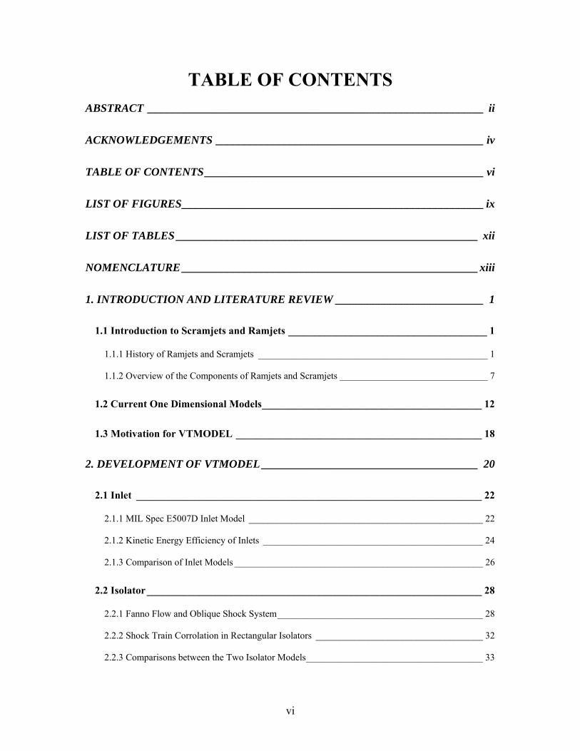
TABLE OF CONTENTS ABSTRACT ___________________________________________________________ ii

ACKNOWLEDGEMENTS _______________________________________________ iv

TABLE OF CONTENTS _________________________________________________ vi

LIST OF FIGURES _____________________________________________________ ix

LIST OF TABLES _____________________________________________________ xii

NOMENCLATURE ____________________________________________________ xiii

1. INTRODUCTION AND LITERATURE REVIEW __________________________ 1

1.1 Introduction to Scramjets and Ramjets ______________________________________ 1

1.1.1 History of Ramjets and Scramjets ________________________________________________ 1

1.1.2 Overview of the Components of Ramjets and Scramjets _______________________________ 7

1.2 Current One Dimensional Models __________________________________________ 12

1.3 Motivation for VTMODEL _______________________________________________ 18

2. DEVELOPMENT OF VTMODEL ______________________________________ 20

2.1 Inlet __________________________________________________________________ 22

2.1.1 MIL Spec E5007D Inlet Model _________________________________________________ 22

2.1.2 Kinetic Energy Efficiency of Inlets ______________________________________________ 24

2.1.3 Comparison of Inlet Models ____________________________________________________ 26

2.2 Isolator ________________________________________________________________ 28

2.2.1 Fanno Flow and Oblique Shock System ___________________________________________ 28

2.2.2 Shock Train Corrolation in Rectangular Isolators ___________________________________ 32

2.2.3 Comparisons between the Two Isolator Models _____________________________________ 33

vii

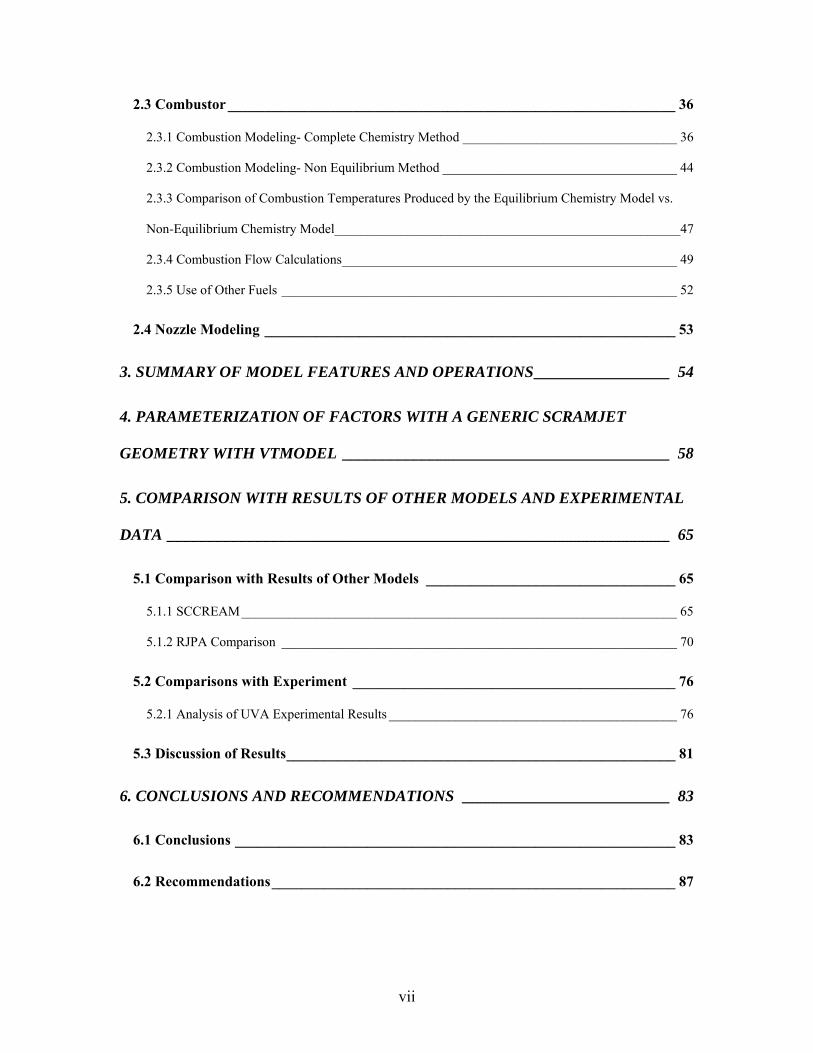
2.3 Combustor _____________________________________________________________ 36

2.3.1 Combustion Modeling- Complete Chemistry Method ________________________________ 36

2.3.2 Combustion Modeling- Non Equilibrium Method ___________________________________ 44

2.3.3 Comparison of Combustion Temperatures Produced by the Equilibrium Chemistry Model vs.

Non-Equilibrium Chemistry Model____________________________________________________47

2.3.4 Combustion Flow Calculations __________________________________________________ 49

2.3.5 Use of Other Fuels ___________________________________________________________ 52

2.4 Nozzle Modeling ________________________________________________________ 53

3. SUMMARY OF MODEL FEATURES AND OPERATIONS _________________ 54

4. PARAMETERIZATION OF FACTORS WITH A GENERIC SCRAMJET

GEOMETRY WITH VTMODEL _________________________________________ 58

5. COMPARISON WITH RESULTS OF OTHER MODELS AND EXPERIMENTAL

DATA _______________________________________________________________ 65

5.1 Comparison with Results of Other Models __________________________________ 65

5.1.1 SCCREAM _________________________________________________________________ 65

5.1.2 RJPA Comparison ___________________________________________________________ 70

5.2 Comparisons with Experiment ____________________________________________ 76

5.2.1 Analysis of UVA Experimental Results ___________________________________________ 76

5.3 Discussion of Results _____________________________________________________ 81

6. CONCLUSIONS AND RECOMMENDATIONS __________________________ 83

6.1 Conclusions ____________________________________________________________ 83

6.2 Recommendations _______________________________________________________ 87

viii

7. REFERENCES _____________________________________________________ 89

7.1 Cited References ________________________________________________________ 89

7.2 Uncited References _____________________________________________________ 94

ix

LIST OF FIGURES

Figure 1-1: Photograph from the 1st ramjet flight (Heiser 1994) ___________________ 2

Figure 1-2: Engine modes vs Mach Number from the SR 71 Flight Manual

(USAF 2002) ___________________________________________________________ 4

Figure 1-3: X-43 Captive and Carry (Kazmar 2005) ____________________________ 5

Figure 1-4: Artist Rendering of the X-51 (Warwick 2010) _______________________ 6

Figure 1-5: Schematic of a Ramjet Engine (Bonanos 2005) ______________________ 7

Figure 1-6: Scramjet Schematic. Courtesy of NASA Langley) ____________________ 8

Figure 1-7: RJPA Schematic (Pandolfini 1992) _______________________________ 13

Figure 1-8: University of Maryland Code Validation (O’Brien T, 2001) ___________ 16

Figure 1-9: University of Adelaide Code Validation with UVA Tunnel Results (Birzer

2009) ________________________________________________________________ 17

Figure 2-1: Station Locations for VTMODEL ________________________________ 21

Figure 2-2: Scramjet Inlet Efficiency from Van Wie (Van Wie 2001) _____________ 24

Figure 2-3: Comparison of Pressure Recoveries vs Flight Mach Number for Three Inlet

Model Calculations _____________________________________________________ 26

Figure 2-4: Sample Static Pressure Profile with marked Fanno Flow and Oblique Shock

Components with VTMODEL Predictions(Rockwell 2010) _____________________ 31

Figure 2-5: Static Pressure Profile for Φ=0.171 obtained by the University of Virginia

(Rockwell 2010) and Static Pressure Predictions by VTMODEL _________________ 33

Figure 2-6: Comparison of Shock Train Correlation Model and Fanno Flow with Oblique

Shock Model- Mach Number _____________________________________________ 34

x

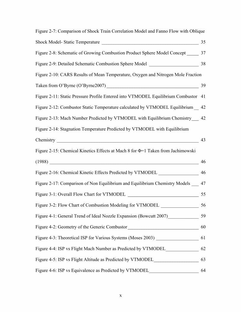
Figure 2-7: Comparison of Shock Train Correlation Model and Fanno Flow with Oblique

Shock Model- Static Temperature _________________________________________ 35

Figure 2-8: Schematic of Growing Combustion Product Sphere Model Concept _____ 37

Figure 2-9: Detailed Schematic Combustion Sphere Model _____________________ 38

Figure 2-10: CARS Results of Mean Temperature, Oxygen and Nitrogen Mole Fraction

Taken from O’Byrne (O’Byrne2007) _______________________________________ 39

Figure 2-11: Static Pressure Profile Entered into VTMODEL Equilibrium Combustor 41

Figure 2-12: Combustor Static Temperature calculated by VTMODEL Equilibrium __ 42

Figure 2-13: Mach Number Predicted by VTMODEL with Equilibrium Chemistry ___ 42

Figure 2-14: Stagnation Temperature Predicted by VTMODEL with Equilibrium

Chemistry ____________________________________________________________ 43

Figure 2-15: Chemical Kinetics Effects at Mach 8 for Φ=1 Taken from Jachimowski

(1988) _______________________________________________________________ 46

Figure 2-16: Chemical Kinetic Effects Predicted by VTMODEL _________________ 46

Figure 2-17: Comparison of Non Equilibrium and Equilibrium Chemistry Models ___ 47

Figure 3-1: Overall Flow Chart for VTMODEL ______________________________ 55

Figure 3-2: Flow Chart of Combustion Modeling for VTMODEL ________________ 56

Figure 4-1: General Trend of Ideal Nozzle Expansion (Bowcutt 2007) _____________ 59

Figure 4-2: Geometry of the Generic Combustor ______________________________ 60

Figure 4-3: Theoretical ISP for Various Systems (Moses 2003) __________________ 61

Figure 4-4: ISP vs Flight Mach Number as Predicted by VTMODEL ______________ 62

Figure 4-5: ISP vs Flight Altitude as Predicted by VTMODEL ___________________ 63

Figure 4-6: ISP vs Equivalence as Predicted by VTMODEL _____________________ 64

xi

Figure 5-1: SCCREAM Combustor Geometry (Bradford 2001) __________________ 66

Figure 5-2: Bradford Comparison of SCCREAM and SRGULL (Bradford 2001) ____ 68

Figure 5-3: VTMODEL Prediction of Bradford Combustor - Mach Number ________ 68

Figure 5-4: ISP vs Mach Number as Predicted by RJPA, SCCREAM (Bradford 2001)

and VTMODEL _______________________________________________________ 71

Figure 5-5: Air Specific Impulse from RJPA (Bonanos 2005) ____________________ 73

Figure 5-6: Air Specific Impulse from RJPA at Various Total Temperatures (Bonanos

2005) ________________________________________________________________ 74

Figure 5-7: Air Specific Impulse Predicted by VTMODEL Overlay over Bonanos

(Bonanos 2005) ________________________________________________________ 74

Figure 5-8: Air Specific Impulse Predicted by VTMODEL for To=1010K Overlay over

Bonanos (Bonanos 2005) ________________________________________________ 75

Figure 5-9: Schematic of UVA Tunnel (Le 2008) _____________________________ 77

Figure 5-10: Static Pressure Predicted by VTMODEL for Φ=0.341 Compared to

VTMODEL ___________________________________________________________ 78

Figure 5-11: Static Temperature Predicted by VTMODEL for Φ=0.341 ____________ 79

Figure 5-12: Mach Number Predicted by VTMODEL for Φ=0.341 _______________ 79

Figure 5-13: Stagnation Temperature Predicted by VTMODEL for Φ=0.341 ________ 80

xii

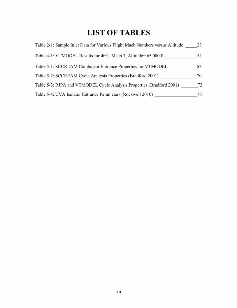
LIST OF TABLES Table 2-1: Sample Inlet Data for Various Flight Mach Numbers versus Altitude _____23

Table 4-1: VTMODEL Results for Φ=1, Mach 7, Altitude= 65,000 ft ______________61

Table 5-1: SCCREAM Combustor Entrance Properties for VTMODEL ____________67

Table 5-2: SCCREAM Cycle Analysis Properties (Bradford 2001) ________________70

Table 5-3: RJPA and VTMODEL Cycle Analysis Properties (Bradford 2001) _______72

Table 5-4: UVA Isolator Entrance Parameters (Rockwell 2010) __________________76

xiii

NOMENCLATURE

A Area

cp Specific Heat at Constant Pressure

dx infinitesimal change in x

x Finite change in x

f Coefficient of Friction

H Enthalpy

Hd Duct Height

h Step size for 4th order RK Method

ho Stagnation Enthalpy per Unit Mass

M Mach Number

M Non Reactive Species in Chemical Equations

Mass Rate of Flow

P Pressure

Pt Total Pressure

Q Net Heat Transfer per Unit Mass of Gas

R Gas Constant

Reθ Reynolds Number Based on Momentum Thickness

S Shock Length

T Static Temperature

To Total Temperature

T Thrust

xiv

TSFC Thrust Specific Fuel Consumption

u5 Exit velocity

um Velocity of Combustible Mixture

uf Combustion Flame Speed

Vflow Bulk Flow Velocity

Ve Nozzle Exit Velocity

w Mass Rate of Flow of Gas Stream

W Molecular Weight

Wx Work

X Drag Force

x Axial Location

Greek

γ Ratio of Specific Heats

θ Boundary Layer Momentum

Thickness

ηn Nozzle Adiabatic Efficiency

xv

Subscripts

a At altitude

0 Inlet Entrance

1 Isolator Entrance

2 Combustor Entrance

3 Combustor Exit

4 Nozzle Exit

s Isentropic

1

Chapter 1

Introduction and Literature Review

1.1 Introduction to Scramjets and Ramjets

1.1.1. History of Ramjets and Scramjets

Ramjets and scramjets are air breathing propulsive engines that rely on the

engine’s forward movement to compress air at the inlet. Scramjets are similar in basic

operating principle to ramjets except that supersonic combustion occurs within the

combustor.

The concept of a ramjet has existed for nearly 100 years. The first ramjet was

proposed by Rene Lorin in 1913 (Heiser 1994). At the time, Lorin realized that there

would be insufficient pressure to operate with subsonic flight. In 1928, a Hungarian

engineer by the name of Albert Fono was issued a German patent on a propulsive device

that has all of the geometric features of a ramjet. The diagram reproduced by the Applied

Physics Laboratory shows a convergent-divergent inlet with a low speed combustor, and

a divergent nozzle. In 1935, Rene Leduc was issued a patent in France for a piloted

aircraft with a ramjet engine. Leduc was not able to build a prototype until the late 1940s

due to the occupation of France during World War II. However, on April 29, 1949, the

first ramjet powered flight was accomplished when the Leduc 010 was launched from a

parent vehicle and achieved Mach 0.84 at 26,000 ft. This historic aircraft is shown in

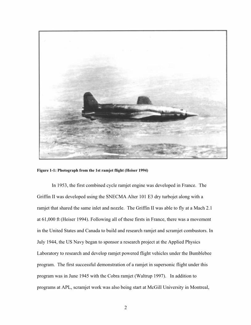
Figure 1-1.

2

Figure 1-1: Photograph from the 1st ramjet flight (Heiser 1994)

In 1953, the first combined cycle ramjet engine was developed in France. The

Griffin II was developed using the SNECMA Alter 101 E3 dry turbojet along with a

ramjet that shared the same inlet and nozzle. The Griffin II was able to fly at a Mach 2.1

at 61,000 ft (Heiser 1994). Following all of these firsts in France, there was a movement

in the United States and Canada to build and research ramjet and scramjet combustors. In

July 1944, the US Navy began to sponsor a research project at the Applied Physics

Laboratory to research and develop ramjet powered flight vehicles under the Bumblebee

program. The first successful demonstration of a ramjet in supersonic flight under this

program was in June 1945 with the Cobra ramjet (Waltrup 1997). In addition to

programs at APL, scramjet work was also being start at McGill University in Montreal,

3

Canada. At McGill, Swithenbank published and reported early work on scramjet inlets,

fuel injection, combustion, and nozzles. Swithenbank focuses on hypersonic flight Mach

numbers of between 10 and 25. In 1958, Weber and MacKay published an analysis on

the feasibility, benefits, and technical challenges to scramjet powered flight (Mach 4-7).

In addition to the work on the Bumblebee project at the Applied Physics Laboratory at

John Hopkins University, Avery and Dugger started an analytical and experimental study

of scramjet engines and the potential in 1957 (Curran 2001). In 1964, Dugger and Billig

submitted a patent application for a scramjet that was based on Billig’s PhD thesis (UMD

2010).

Ramjets have also been combined with turbine engines for high speed flight.

Perhaps the most famous combined cycle aircraft is the SR-71. The SR-71 was

developed in the early 1960s at Lockheed Martin’s Skunk Works facility (Lockheed

Martin 2010). The aircraft had a Pratt and Whitney J58-P4 power system on board. The

J58-P4 is a hybrid turbine-ramjet engine. At lower speeds, the engine was flown as a

turbojet. At supersonic speeds, the engine then flew in “ramjet mode”. The engine was

essentially a turbojet inside of a ramjet (Goodall 2002). Figure 1.2 shows the operational

modes of the J-58 at increasing flight Mach numbers.

4

Figure 1-2: Engine modes vs. Mach Number from the SR 71 Flight Manual (USAF 2002)

The evolution of the scramjet engine was to follow the success of ramjets in aircraft and

missile systems. To follow the earlier work in scramjet research, the National Aerospace

Plane project (X-30) envisioned a single stage space access plane. This project was

started in the 1980s and was funded by both NASA and the DOD with additional support

from DARPA. The plane was to incorporate a scramjet engine powered by hydrogen.

Unfortunately, the National Aerospace Plane project was canceled in 1993 before a

5

prototype could be built. Some of the research and development for the X-30 was then

used for the X-43 hydrogen-fueled hypersonic research aircraft. The X-43 was designed

and built to be an unmanned system. A Pegasus booster launched from a B-52 was used

to achieve to the correct altitude and speed prior to igniting the X-43 scramjet engine. In

2004, the X-43 was able to reach and maintain a record speed of Mach 9.68 at 112,000 ft

(Kazmar 2005).

Figure 1-3: X-43 Captive and Carry (Kazmar 2005)

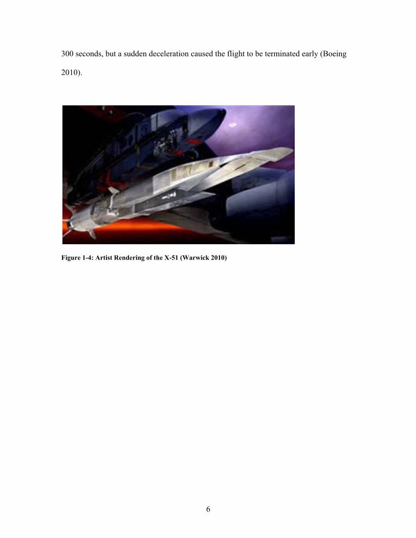
Most recently, an advancement of scramjet-powered vehicle occurred with the

successful test of the X-51. The X-51, an integrated rocket-boosted and scramjet vehicle,

was developed by Boeing in partnership with the USAF, DARPA, NASA, and Pratt and

Whitney Rocketdyne. The scramjet fuel was the hydrocarbon JP-7. On May 26, 2010,

the X-51 had a successful first flight. The research vehicle was launched from a B-52.

The X-51 broke the record for the longest scramjet-powered flight, operating for over 200

seconds. The X-51 reached Mach 5 in its first flight. The flight was planned to be over

6

300 seconds, but a sudden deceleration caused the flight to be terminated early (Boeing

2010).

Figure 1-4: Artist Rendering of the X-51 (Warwick 2010)

7

1.1.2. Overview of the Components of Ramjets and Scramjets

Ramjets and scramjets, unlike turbomachinery-based engines, have no moving

parts and consist of a basic inlet, isolator, combustor, and nozzle. These components are

pictured in Figure 1-5 and 1-6. Figure 1-5 is a basic schematic of a ramjet engine, while

Figure 1-6 represents a scramjet engine.

Figure 1-5: Schematic of a Ramjet Engine (Bonanos 2005)

8

Figure 1-6: Scramjet Schematic Courtesy of NASA Langley

From the figures it can be seen that the first component of a ramjet or a scramjet

is the inlet. These supersonic inlets can be of many shapes and designs, but the overall

function is the same. The inlet reduces the Mach number and compresses the inlet air to

a desired state prior to isolator or combustor entry. According to Segal (Segal 2009),

inlets for a scramjet can either be fixed or contain adjustable surfaces. Ramjet inlets for

aircraft up to Mach 2 flight conditions can generally be considered to be fixed, however

at higher Mach numbers, a variable geometry inlet may be required. An exception to this

may be in the case of a missile or a combined cycle missile. In general, a fixed geometry

inlet must be of a design that provides adequate flow compression for inlet start. For

other vehicle applications, the inlet may require adjustable surfaces for starting and to

control the compression of the flow for off- design engine operation (Segal 2009).

9

There are five features that scramjets inlets will likely contain: (1) All of the

design surfaces are used to compress the flow, resulting in a complicated 3D shock

system; (2) Adjustable surfaces and variable geometry are used to support flights from

supersonic to hypersonic speeds; (3) The inlet through the use of an isolator will have to

be “compatible” with the combustion pressure rise; (4) The inlet must be integrated with

the fuselage design to accommodate the long compression ramps; (5) Finally, the inlet

will be “arranged in a single segment or in several segments” to optimize the frontal area

(Segal 2009).

The isolator is an essential part of any scramjet engine. The isolator is a constant

cross sectional area duct that is designed to prevent unstart of the inlet. With supersonic

combustion, the isolator shock train that is created by the pressure demand of the

combustion process can move forward in the inlet, disrupting the inlet function. This can

cause failure of the engine. The isolator is designed to contain this shock train,

preventing it from unstarting the inlet.

The combustor of the scramjet encloses supersonic combustion. In a ramjet or a

dual mode scramjet this process can also occur at or below the local speed of sound. The

combustor is generally made up of an igniter, fuel injectors, and a flame holder. The

igniter can vary in design with the use of silane, a shock detonator tube, solid propellant

igniters, or a plasma torch such as the Virginia Tech Plasma Torch (Bonanos 2005).

Some engines have been tested that do not have a definitive igniter, but depend on the

fuel auto ignition characteristics, typically of hydrogen fuel. The fuel injectors can be

located either upstream or downstream of the igniter depending on the design. The flame

holder can be a cavity built into the geometry of the combustor, a flow ramp in the flow

10

path, or a flush-wall device such as the Virginia Tech Plasma Torch (Bonanos 2005).

The cavity provides flame holding by incorporating a stationary combustion recirculation

region for continuously igniting the fuel-air mixture. Combustors are generally expanding

in flow area to maintain the flow Mach number at the desired levels.

Within the combustor of a scramjet, there are multiple design issues that must be

considered (Schetz 2007):

Wall shear

Base pressure drag

Injector drag

Heat transfer through the walls

Isolator pressure rise

Peak heat flux

Rayleigh irreversibility

Incomplete mixing and combustion

Flow distortion

Chemical dissociation

Combustor pressure rise

These design issues are categorized to include momentum, energy, cycle efficiency, and

operability effects.

The nozzle of a scramjet has its own requirements for expansion of flow. In a

scramjet design, the enthalpy of the flow should have increased enough by the

combustion process to produce thrust. The nozzle is generally a divergent duct to expand

the flow, typically with a continuing combustion reaction because of the low residence

11

time of the fuel and air within the combustor. Due to the fact that scramjets require a

large nozzle pressure ratio, Segal states that nozzles should be of the “open type” (Segal

2009). This open type is defined as using the aft vehicle surface as part of the nozzle,

instead of a separate independent duct. Since the thrust of the engine is only slightly

greater than the vehicle’s drag at hypersonic speeds, good efficiency and design of the

nozzle is essential to the success of the engine (Segal 2009).

12

1.2 Current One-Dimensional Models

One- dimensional scramjet flowpath analysis codes can be a useful analytical tool

for scramjet researchers and designers. There are many advantages to the appropriate use

of a one-dimensional code versus a more complex two or three dimensional flow analysis

such as CFD. These advantages include faster computational times and easier overall

performance-based analysis. Though the analysis cannot predict effects of boundary

layers and other multidimensional flow properties, the one-dimensional code can provide

reasonable ranges for thermodynamic and performance design criteria.

One of the legacy codes widely used for the one-dimensional simulation of

scramjets and ramjets is the Ramjet Performance Analysis Code (RJPA). This code was

developed at the Applied Physics Laboratory at John Hopkins University, and is

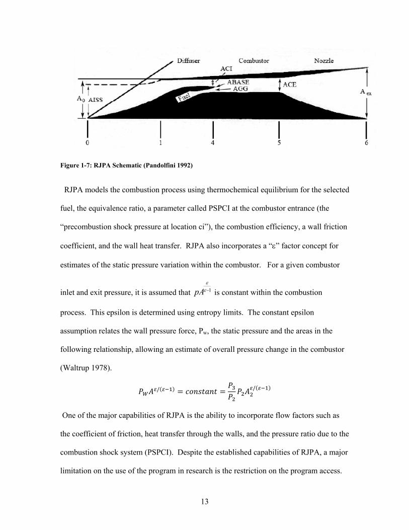
considered the industry standard. The code separates the flow path into major sections

designated the Freestream, Diffuser, Combustor, and Nozzle. Each one of these

components is modeled as a control volume with data passing across the boundaries.

Figure 1-7 below shows the basic schematic of RJPA. The numbers below the schematic

are the locations where the program calculates thermodynamic data.

13

Figure 1-7: RJPA Schematic (Pandolfini 1992)

RJPA models the combustion process using thermochemical equilibrium for the selected

fuel, the equivalence ratio, a parameter called PSPCI at the combustor entrance (the

“precombustion shock pressure at location ci”), the combustion efficiency, a wall friction

coefficient, and the wall heat transfer. RJPA also incorporates a “” factor concept for

estimates of the static pressure variation within the combustor. For a given combustor

inlet and exit pressure, it is assumed that 1

pA is constant within the combustion

process. This epsilon is determined using entropy limits. The constant epsilon

assumption relates the wall pressure force, Pw, the static pressure and the areas in the

following relationship, allowing an estimate of overall pressure change in the combustor

(Waltrup 1978).

/ /

One of the major capabilities of RJPA is the ability to incorporate flow factors such as

the coefficient of friction, heat transfer through the walls, and the pressure ratio due to the

combustion shock system (PSPCI). Despite the established capabilities of RJPA, a major

limitation on the use of the program in research is the restriction on the program access.

14

The program is considered ITAR restricted. This restriction makes the access and use of

the program out of the public domain.

One scramjet analysis program that is in the public domain is known as HAP

(Hypersonic Airbreathing Propulsion). The program accompanies a text by Heiser and

Pratt called Hypersonic Airbreathing Propulsion (Heiser 1994). This text is part of an

AIAA educational series. HAP is written in MS DOS and will run on most computers in

the command prompt. Some of the features and analysis capabilities of HAP are the

ability to perform trajectory analysis and calculate the overall performance of scramjets,

and the use of compressible flow and isentropic flow properties for calorically perfect

gasses. The program also assumes a simplified ideal chemical equilibrium in the

combustor. These assumptions make HAP inaccurate for use at higher Mach numbers.

There is no visual interface in HAP. The inputs are in a text file (Heiser 1994).

A program developed in the late 1980s for one-dimensional scramjet analysis at

the NASA Glenn Research Center is called RAMSCRAM. The program uses chemical

thermodynamic equilibrium for the combustion modeling (Burkardt 1990). The program

allows for multiple fuel injectors and multiple compressors sections (Bradford 2001).

The most recent development of a scramjet performance code at the NASA

Langley Research Center is the code SRGULL (Zweber 2002). This program uses

multiple subroutines for each section of the combustor. The program uses 1-D, and 2-D

modeling for the flow path. The inlet and nozzle subroutines use 2-D modeling. This

modeling is called “axisymmetric with 3-D corrections.” For the combustor modeling,

SRGULL uses a one-dimensional equilibrium model.

15

Another one-dimensional code is SCCREAM developed at Georgia Tech

(Bradford 1998). SCCREAM stands for Simulated Combined-Cycle Rocket Engine

Analysis Module. This program is written in C++, and was developed to provide a

conceptual design tool for analyzing rocket and scramjet combined systems. One of the

advantages of this code is the fact that it can “run a full range of flight conditions and

engine modes in under 60 seconds, and will output a properly formatted POST engine

table” (Bradford 1998). The SCCREAM code results from Bradford’s dissertation will

be used as a comparison tool for VTMODEL results in Chapter 5.

An addition to combined cycle codes was developed at the University of

Maryland by O’Brien et al (O’Brien, T 2001). In this code, finite rate chemistry of

hydrogen and Jet A were coupled with flow equations to model combustors in scramjets

combustors. Since chemical kinetics is used, fuel ignition and combustion progress can

be predicted and modeled. This is a benefit of this code versus chemical equilibrium

codes. The Jachimowski reaction was used for hydrogen chemical kinetics

(Jachimowski 1988), while the Kundu reaction was used for Jet A (Lee 1991). For

modeling of the chemical kinetics, the model uses Chemkin II (Reaction Design 2010).

Chemkin is a commercial software product that integrates chemical kinetics into

simulations of reacting flow. The University of Maryland code was also validated by

comparisons of predicted static pressure versus experimental pressure profiles. Figure 1-8

shows one the comparison with experimental results obtained by Billig.

16

Figure 1-8: University of Maryland Code Validation (O'Brien T, 2001)

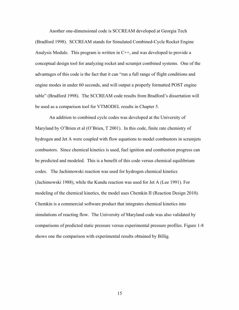
Another model created at the University of Adelaide in Australia was used to

analyze the University of Virginia Direct Connect Tunnel results (Birzer 2009). The

model uses a quasi – one-dimensional solver that assumes that the flow is steady state,

ideal gas, and that flow properties are quasi-one dimensional. One of the weaknesses of

the program is that the combustion is assumed to be only mixing-limited instead of

including kinetics limitations. This assumption lowers the computational time, but the

effect on the analysis results is not noted in the paper. The code has been validated by

comparisons of predicted pressures to experimental static pressures. Figure 1-9 shows a

result with good agreement for hydrogen fuel combustion with =0.32.

17

Figure 1-9: University of Adelaide Code Validation with UVA Tunnel Results (Birzer 2009)

18

1.3 Motivation for VTMODEL

From the above review it can be seen that there are many one-dimensional codes

available for the analysis of scramjet and ramjet flowpaths. Some of the reviewed codes

are combined cycle codes, offering the additional benefit of being able to analyze the

performance of such vehicles from launch. The present research provides an additional

code for the modeling of scramjet performance, named VTMODEL. The main

motivation behind VTMODEL was to provide a capable, user friendly code with

thermodynamic analysis capabilities, for use in the public domain.

VTMODEL was developed to make an accessible analysis code that can be

modified and improved by the user. Since the program is not a compiled code, the user

can add or change the main functions and tailor the code to their requirements.

VTMODEL was also developed to make the analysis solution more adaptable to different

test requirements. The program can be both predictive and analytic; that is, an internal

static pressure profile from experimental data can be entered in and analyzed. The

alternative “predictive” solution method iterates on a solution until a specified combustor

exit pressure or nozzle exit pressure condition is met.

The analysis modules of VTMODEL provide flow path computations for given

flight conditions, and specified Isolator, Combustion, Combustor Flow, and Nozzle

parameters. Within these major functions, the user has options of which of the included

alternate models to use. For the isolator function, there are two flow models based on

correlation data from Sullins and McLafferty (Sullins 1992), and a more analytical Fanno

flow model combined with an oblique shock system model. The combustion function

also has available two different analyses. The first model is a complete combustion

19

(equilibrium) combustion solver with an “expanding combustion sphere” efficiency

model. The second model is a non-equilibrium hydrogen combustion solver using a

mechanism developed by Jachimowski (Jachimowski 1988).

20

Chapter 2

Development of VTMODEL As mentioned, the development of VTMODEL addressed an internal need for a

public access one-dimensional ramjet and scramjet analysis code. The model was created

to provide flexibility to the user in choosing different models for the inlet, isolator, and

combustor. The basis of the model is a segmented approach to the analysis of the flow

within each component of the ramjet and scramjet. Each individual module can be

modified and adapted, providing flexibility to expand on the model and apply the model

to the user’s specific criteria. For the flow entering the inlet, the properties are calculated

from given flight conditions.

For the isolator with given inlet flow conditions, the model requires a static

pressure anchor at an axial location in the combustor or the nozzle exit. This static

pressure anchor is necessary for establishing the required static pressure rise in the

isolator. The supersonic combustion process, the flow area of the combustor and nozzle,

and the friction and heat transfer in the combustor together establish the required

combustor inlet Mach number for a given inlet pressure and temperature. This

combustor inlet flow state must match the exit condition from the isolator. To calculate

and quantify this effect in the isolator, the shock train length or the oblique shock angles

are iterated upon to provide the required combustor inlet conditions. It is necessary for a

static pressure anchor to be identified and set downstream of the isolator. Example

anchor points are the combustor entrance, combustor exit, or nozzle exit. If no other

21

information is available, the nozzle exit static pressure is equated to atmospheric

conditions. This results in a flow prediction based on an ideally-expanded nozzle.

The required isolator flow properties are used by the isolator model calculation

process. For one option of the module, VTMODEL assumes the longest shock length

possible, which is the isolator length. The program then lowers this value to match the

isolator discharge static pressure anchor. This procedure is similar to that for the second

option, which iterates on the reflected shock angles. This iteration is necessary for the

isolator pressure rise to have a proper match to the flow conditions in the combustor.

The overall model uses the subscripts given in Figure 2-1 for thermodynamic data

locations. Positions 0 and 1 designate the entrance and exit of the inlet. The isolator

entrance and exit is designated by locations 1 and 2. The combustor entrance is

designated as location 2 and the exit is location 3. The exit of the nozzle is location 4. An

additional subscript is used for atmospheric conditions.

Figure 2-1: Station Locations for VTMODEL

22

2.1 Inlet Modeling

The inlet function requires an input of the flight altitude and Mach number to set

the upstream boundary condition. VTMODEL l uses the US Standard Atmosphere

properties at altitudes specified every 5,000 feet (US Government Printing Office 1976).

The incoming flight Mach number (Mo) is defined by the user and is used for determining

supersonic inlet pressure recovery.

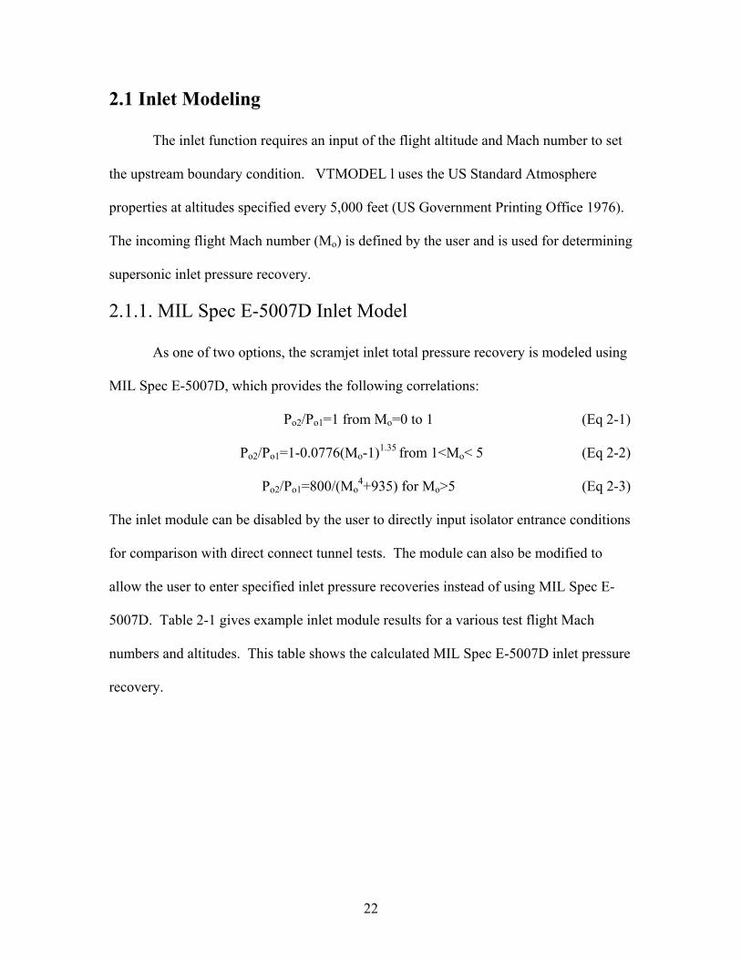
2.1.1. MIL Spec E-5007D Inlet Model

As one of two options, the scramjet inlet total pressure recovery is modeled using

MIL Spec E-5007D, which provides the following correlations:

Po2/Po1=1 from Mo=0 to 1 (Eq 2-1)

Po2/Po1=1-0.0776(Mo-1)1.35 from 1<Mo< 5 (Eq 2-2)

Po2/Po1=800/(Mo4+935) for Mo>5 (Eq 2-3)

The inlet module can be disabled by the user to directly input isolator entrance conditions

for comparison with direct connect tunnel tests. The module can also be modified to

allow the user to enter specified inlet pressure recoveries instead of using MIL Spec E-

5007D. Table 2-1 gives example inlet module results for a various test flight Mach

numbers and altitudes. This table shows the calculated MIL Spec E-5007D inlet pressure

recovery.

23

Flight Mach Number Altitude (ft) Ta(K) M1 T1(K)

Pressure RecoveryP02/P01

5 50,000 217 4.42 265 0.51

5 60,000 217 4.42 265 0.51

5 70,000 218 4.42 267 0.51

5 80,000 221 4.42 270 0.51

6 50,000 217 5.06 290 0.36

6 60,000 217 5.06 290 0.36

6 70,000 218 5.06 292 0.36

6 80,000 221 5.06 296 0.36

7 50,000 217 5.56 326 0.24

7 60,000 217 5.56 326 0.24

7 70,000 218 5.56 328 0.24

7 80,000 221 5.56 332 0.24

8 50,000 217 5.98 366 0.16

8 60,000 217 5.98 366 0.16

8 70,000 218 5.98 369 0.16

8 80,000 221 5.98 374 0.16

9 50,000 217 6.35 411 0.11

9 60,000 217 6.35 411 0.11

9 70,000 218 6.35 413 0.11

9 80,000 221 6.35 419 0.11

10 50,000 217 6.69 457 0.07

10 60,000 217 6.69 457 0.07

10 70,000 218 6.69 460 0.07

10 80,000 221 6.69 466 0.07

Table 2-1: Sample Inlet Data for Various Flight Mach Numbers versus Altitude

24

2.1.2. Kinetic Energy Efficiency of Inlets

An additional inlet model specifically designed for scramjet application was

added to VTMODEL based on the compilation of inlet information in the Van Wie

section of Scramjet Propulsion (Van Wie 2001). Van Wie used experimental

correlations for kinetic energy efficiency from various experimental results. The data and

his correlations are shown in Figure 2-2 below.

Figure 2-2: Scramjet Inlet Efficiency from Van Wie (Van Wie 2001)

25

From this efficiency chart, the following equations can be selected as the kinetic energy

efficiency correlations:

1 0.528 1 / . (Eq 2-4)

1 0.4 1 / (Eq 2-5)

The kinetic energy efficiency correlation is then used to find the pressure recovery in the

inlet. The following equation is then used to find the value of the stagnation pressure

recovery.

(Eq 2-6)

1

1

020

0

120 2

11

1

2

o

o

o

oKE P

PM

T

T

M

26

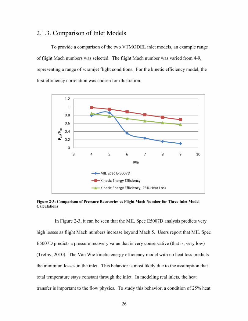
2.1.3. Comparison of Inlet Models

To provide a comparison of the two VTMODEL inlet models, an example range

of flight Mach numbers was selected. The flight Mach number was varied from 4-9,

representing a range of scramjet flight conditions. For the kinetic efficiency model, the

first efficiency correlation was chosen for illustration.

Figure 2-3: Comparison of Pressure Recoveries vs Flight Mach Number for Three Inlet Model Calculations

In Figure 2-3, it can be seen that the MIL Spec E5007D analysis predicts very

high losses as flight Mach numbers increase beyond Mach 5. Users report that MIL Spec

E5007D predicts a pressure recovery value that is very conservative (that is, very low)

(Trefny, 2010). The Van Wie kinetic energy efficiency model with no heat loss predicts

the minimum losses in the inlet. This behavior is most likely due to the assumption that

total temperature stays constant through the inlet. In modeling real inlets, the heat

transfer is important to the flow physics. To study this behavior, a condition of 25% heat

0

0.2

0.4

0.6

0.8

1

1.2

3 4 5 6 7 8 9 10

Po1/P

o0

Ma

MIL Spec E‐5007D

Kinetic Energy Efficiency

Kinetic Energy Efficiency, 25% Heat Loss

27

loss (T02/T01=0.75) was assumed in the inlet. The effect on the pressure recovery

prediction can be seen in Figure 2-3. This solution falls between the ideal kinetic energy

efficiency model and the MIL Spec model. The heat transfer can be predicted by using

Reynolds Analogy. The model is presented in Chapter 2.3.4.

28

2.2 Isolator Modeling

2.2.1. Fanno Flow and Oblique Shock System

Depending on the type of flow solution desired, the VTMODEL isolator models

can be used to predict local flow properties in the isolator. If a static pressure profile is

given from an experiment (referred to as “user supplied”), the models can be used to

predict local temperatures and Mach numbers. If the model is predictive, the isolator

flow variables become part of a system iteration which is ultimately anchored by the

nozzle exit pressure.

Within VTMODEL, there are two isolator flow models that the user can choose.

The first model is comprised of two separate components. The initial component enables

modeling of pressure rise due to friction. The model uses the Fanno flow relationships

(Hill and Peterson 1992, pp. 77-84) to calculate the pressure rise due to friction in a

constant cross sectional area. The following relationship initiates the calculation based

on the length x of the isolator and the lengths L* from stations 1 and x, respectively, to

the sonic (M=1) state.

∗ ∗

(Eq 2-7)

where cf =0.0015 is the VTMODEL default value and can be changed by the user.

The static pressure rise due to friction can be either determined from the

previously mentioned user-supplied static pressure profile or iterated as a contributing

factor to the combustor/nozzle exit pressure. Using the Fanno flow model, the values of

29

cf, ϒ, isolator length L and hydraulic diameter D, and inlet M determine the pressure

change.

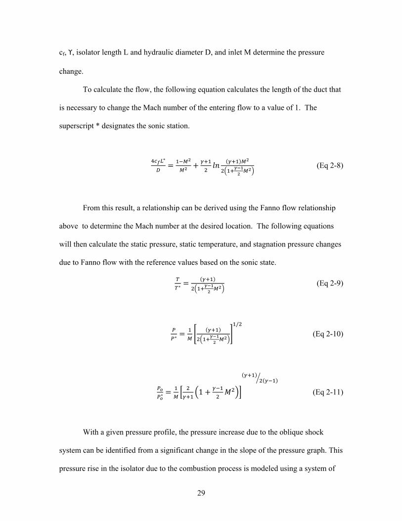
To calculate the flow, the following equation calculates the length of the duct that

is necessary to change the Mach number of the entering flow to a value of 1. The

superscript * designates the sonic station.

∗

(Eq 2-8)

From this result, a relationship can be derived using the Fanno flow relationship

above to determine the Mach number at the desired location. The following equations

will then calculate the static pressure, static temperature, and stagnation pressure changes

due to Fanno flow with the reference values based on the sonic state.

∗ (Eq 2-9)

∗

/

(Eq 2-10)

∗ 1 (Eq 2-11)

With a given pressure profile, the pressure increase due to the oblique shock

system can be identified from a significant change in the slope of the pressure graph. This

pressure rise in the isolator due to the combustion process is modeled using a system of

30

two oblique shocks. When the overall static pressure ratio is input by the user, the shock

angles of the reflected oblique shock system can be calculated. From these angles, the

Mach number and temperature following each shock are calculated.

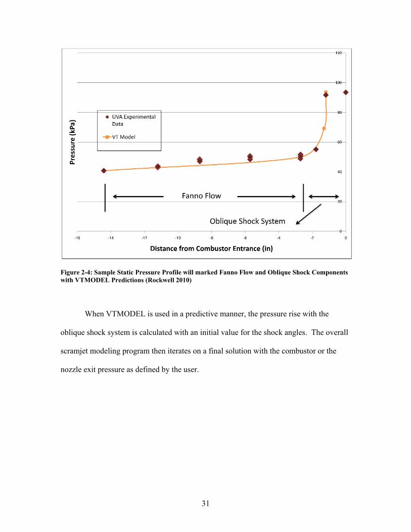
To demonstrate the segmentation of the static pressure profile into Fanno flow

and oblique shock-modeled portions, Figure 2-4 below is given as an example. The static

pressure data was obtained from the University of Virginia Direct Connect tunnel

(Rockwell 2010). The isolator has a constant cross sectional area. As can be seen from

Figure 2-4, approximately 10 kPa of the total pressure rise is modeled by Fanno flow,

while the remaining 45 kPa pressure rise is modeled by the oblique shock system.

31

Figure 2-4: Sample Static Pressure Profile will marked Fanno Flow and Oblique Shock Components with VTMODEL Predictions (Rockwell 2010)

When VTMODEL is used in a predictive manner, the pressure rise with the

oblique shock system is calculated with an initial value for the shock angles. The overall

scramjet modeling program then iterates on a final solution with the combustor or the

nozzle exit pressure as defined by the user.

32

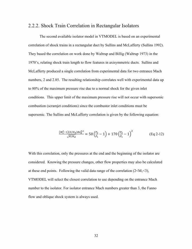
2.2.2. Shock Train Correlation in Rectangular Isolators

The second available isolator model in VTMODEL is based on an experimental

correlation of shock trains in a rectangular duct by Sullins and McLafferty (Sullins 1992).

They based the correlation on work done by Waltrup and Billig (Waltrup 1973) in the

1970’s, relating shock train length to flow features in axisymmetric ducts. Sullins and

McLafferty produced a single correlation from experimental data for two entrance Mach

numbers, 2 and 2.85. The resulting relationship correlates well with experimental data up

to 80% of the maximum pressure rise due to a normal shock for the given inlet

conditions. This upper limit of the maximum pressure rise will not occur with supersonic

combustion (scramjet conditions) since the combustor inlet conditions must be

supersonic. The Sullins and McLafferty correlation is given by the following equation:

/ .

/50 1 170 1 (Eq 2-12)

With this correlation, only the pressures at the end and the beginning of the isolator are

considered. Knowing the pressure changes, other flow properties may also be calculated

at these end points. Following the valid data range of the correlation (2<M1<3),

VTMODEL will select the closest correlation to use depending on the entrance Mach

number to the isolator. For isolator entrance Mach numbers greater than 3, the Fanno

flow and oblique shock system is always used.

33

2.2.3. Comparisons between the Two Isolator Models

Figure 2-6 and 2-7 below show an example isolator module run based on previously

shown experimental pressure data obtained from the University of Virginia dual mode

combustion test facility for an equivalence ratio Φ=0.171 (Rockwell 2010). The input

static pressure profile is shown in Figure 2-5 below.

Figure 2-5: Static Pressure Profile for Φ=0.171 obtained by the University of Virginia (Rockwell 2010) and Static Pressure Predictions by VTMODEL

0

10

20

30

40

50

60

70

80

90

100

1 1.1 1.2 1.3 1.4 1.5 1.6 1.7 1.8 1.9 2

Static Pressure (kPa)

Station

UVA Experimental Data

VTMODEL, Fanno Flow and Oblique Shocks

VTMODEL, Shock Train Correlation

34

Figure 2-6: Comparison of Shock Train Correlation Model and Fanno Flow with Oblique Shock Model - Mach Number

As can be seen from Figure 2-6, the resulting isolator exit Mach numbers vary widely

depending on what isolator program is used. For the same given pressure rise, the shock

train correlation model gives a subsonic condition, while the Fanno flow and oblique

shock correlation predict a supersonic Mach number. For an entrance Mach number of 2,

a normal shock would give an exit Mach number of 0.5774 (John 1984). Therefore,

despite the subsonic Mach number, the resulting value still shows pressure rise below the

strength of a normal shock.

From both Figures 2-6 and 2-7 it can be seen that the predicted combustor

entrance flow properties are highly dependent on the isolator modeling method that is

1 1.1 1.2 1.3 1.4 1.5 1.6 1.7 1.8 1.9 20.8

1

1.2

1.4

1.6

1.8

2

2.2

Station

Mac

h N

umbe

r

Shock Train Correlation Model

Fanno Flow with Oblique Shock

35

used. Both models are included in the final VTMODEL to allow the user to pick the

isolator model that best models their scramjet/ramjet engine flowpath.

Figure 2-7: Comparison of Shock Train Correlation Model and Fanno Flow with Oblique Shock Model - Static Temperature

1 1.1 1.2 1.3 1.4 1.5 1.6 1.7 1.8 1.9 2700

750

800

850

900

950

Station

Sta

tic T

empe

ratu

re (

Kel

vin)

Shock Train Correlation Model

Fanno Flow with Oblique Shock

36

2.3 Combustor Modeling

Two options for calculating the combustion process are offered in VTMODEL. A

unique method is developed based on a local combustion efficiency model, the complete

combustion of the injected fuel in the combustor with the progress of the reaction

controlled by the local combustion efficiency, and the use of compressible flow influence

coefficients to calculate the local Mach number and other flow properties in the

combustor. This method is computationally fast, provides local flow properties at any

desired spacing, and can be applied to any fuel.

A second method based on the work of Jachimowski (Jachimowski 1998) is

implemented. This finite rate combustion model incorporates a set of reduced-order

hydrogen combustor chemistry equations, and is therefore limited to the use of hydrogen

fuel in the combustor.

2.3.1. Combustion Modeling; Complete Combustion Method

The scramjet combustor is modeled using a complete combustion model, a flame

speed model, and an influence coefficient compressible flow calculation. Here, complete

combustion is defined as an immediate fuel and air reaction yielding only the completely

oxidized combustion products and the remaining fuel or oxidizer, with no dissociation of

combustion product species.

37

Using the model, the combustion temperature prediction is the result of successive

combustion calculations in sections over the length of the combustor.

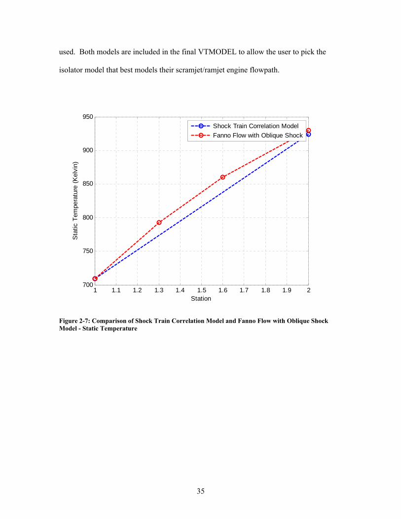
The flame speed model is used to determine the amount of fuel that is burned in

each section, providing a combustion efficiency input. The flame speed model calculates

the “fuel-air combustion sphere” produced by fuel injection into the flowpath., shown

conceptually in Figure 2.8.

The model is based on an approach presented in a text by Hill and Peterson (Hill 1975).

The combustion flame speed is set to an appropriate level (between 40-80 m/s for

hydrogen). Complete mixing of the fuel and air at the injection point is assumed. The

growth of the projected area of the combustion sphere relative to the local cross sectional

of the combustor is taken as the amount of fuel burned in a section, and therefore the

local combustion efficiency. For the combustion calculation, the equivalence ratio along

with the combustion sphere model determines the moles of fuel burned in the section.

Figure 2-8: Schematic of Growing Fuel-Air Combustion Product Sphere Model Concept

38

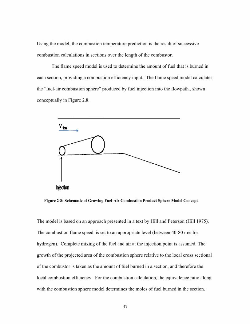
Figure 2-9 below shows the geometry of the combustion sphere model.

Figure 2-9: Detailed Schematic of Combustion Sphere Model

In the figure, α designates the cone angle of the flame front, um designates the velocity of

the combustible mixture, and uf designates the flame speed. The two velocities define the

cone angle:

(Eq 2-13)

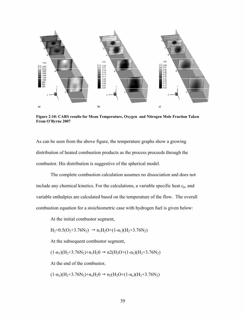
Although the combustion sphere model clearly involves simplifying assumptions,

the model is conceptually supported by experimental data obtained using the coherent

anti-Stokes Raman scattering (CARS) method (O’Bryne 2007). This method was used to

measure temperature and hydrogen combustion species in the NASA Langley Research

Center’s Direct Connect Tunnel. The results of the experiment are in Figure 2-10 below.

39

Figure 2-10: CARS results for Mean Temperature, Oxygen and Nitrogen Mole Fraction Taken From O’Byrne 2007

As can be seen from the above figure, the temperature graphs show a growing

distribution of heated combustion products as the process proceeds through the

combustor. His distribution is suggestive of the spherical model.

The complete combustion calculation assumes no dissociation and does not

include any chemical kinetics. For the calculations, a variable specific heat cp, and

variable enthalpies are calculated based on the temperature of the flow. The overall

combustion equation for a stoichiometric case with hydrogen fuel is given below:

At the initial combustor segment,

H2+0.5(O2+3.76N2) n1H2O+(1-n1)(H2+3.76N2)

At the subsequent combustor segment,

(1-n1)(H2+3.76N2)+n1H20 n2(H2O+(1-n2)(H2+3.76N2)

At the end of the combustor,

(1-nx)(H2+3.76N2)+nxH20 n2(H2O+(1-nx)(H2+3.76N2)

40

where 0<nx<1, controlled by the combustion efficiency derived from the

combustion sphere model.

At a given combustor segment location, the amount of hydrogen burned and the

proportion of air and water for the reactants is thus known. The temperature change of

the combustion products in the segment may then be calculated as the adiabatic flame

temperature for the segment reaction, using the First Law of Thermodynamics.

H2-H1=0 (Eq 2-14)

expanding the above equation yields

∑ ∑

0 0 0 (Eq 2-15)

where (Hx-Hy)=cp(Tx-Ty)

where T1 designates the temperature at the segment inlet, and T2 designates the

segment outlet adiabatic flame temperature. The subscript 0 designates the base

reference state of 298K.

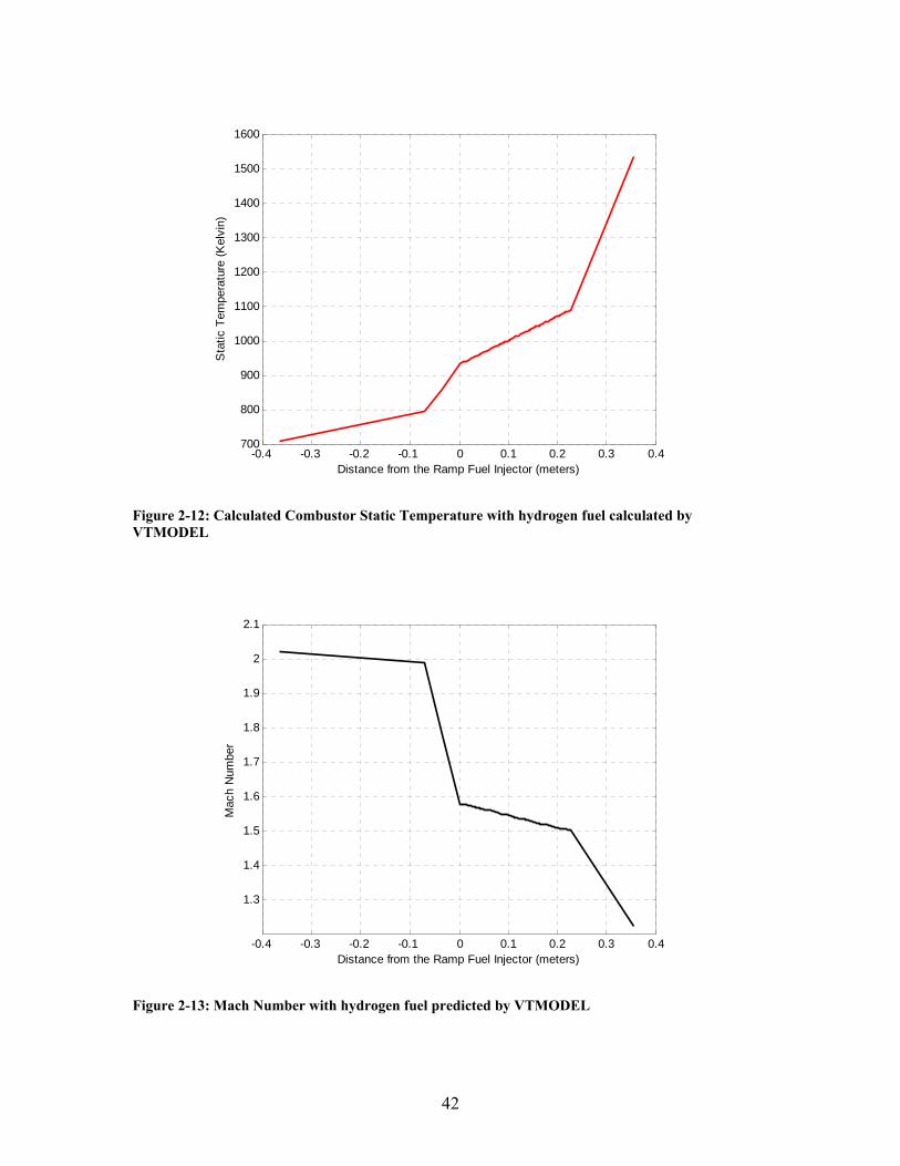
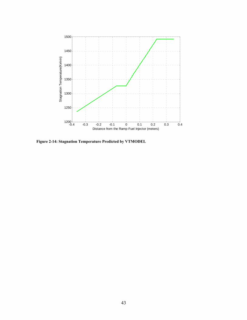
Figures 2-11 to 2-14 show an example calculation for a combustor using complete

combustion for hydrogen. In this case, an assumed pressure profile was entered into

VTMODEL. This pressure profile is shown in Figure 2-11. The Fanno flow and oblique

shock isolator model was used for the isolator to match the given combustor inlet

pressure, which resulted in the combustor inlet temperature and Mach number. For the

equilibrium chemistry calculation, a combustion efficiency of 70% was assumed. This

efficiency resulted from a flame speed of 76 m/s.

41

With the combustor temperature and pressures, the local Mach numbers and other

flow variables in the combustor were then calculated using the influence coefficient

method to be described in Section 2.3.4. This procedure yielded a complete prediction

for the flow states in the combustor as shown in Figures 2-12 to 2-14.

Figure 2-11: Static Pressure Profile Entered into VTMODEL Complete Combustion Model

-0.4 -0.3 -0.2 -0.1 0 0.1 0.2 0.3 0.440

50

60

70

80

90

100

110

120

Distance from the Ramp Fuel Injector (meters)

Sta

tic P

ress

ure

(kP

a)

42

Figure 2-12: Calculated Combustor Static Temperature with hydrogen fuel calculated by VTMODEL

Figure 2-13: Mach Number with hydrogen fuel predicted by VTMODEL

-0.4 -0.3 -0.2 -0.1 0 0.1 0.2 0.3 0.4700

800

900

1000

1100

1200

1300

1400

1500

1600


Sta

tic T

empe

ratu

re (

Kel

vin)

-0.4 -0.3 -0.2 -0.1 0 0.1 0.2 0.3 0.4

1.3

1.4

1.5

1.6

1.7

1.8

1.9

2

2.1


Mac

h N

umbe

r

43

Figure 2-14: Stagnation Temperature Predicted by VTMODEL

-0.4 -0.3 -0.2 -0.1 0 0.1 0.2 0.3 0.41200

1250

1300

1350

1400

1450

1500


Sta

gnat

ion

Tem

pera

ture

(Kel

vin)

44

2.3.2 Combustion Modeling; Non Equilibrium Method

Due to the limitations of the complete combustion model, a finite rate hydrogen

combustion module was implemented in VTMODEL using simplified chemical kinetics

and non-equilibrium hydrogen chemistry. This model was based on the work done by

Jachimowski on the analytical study of hydrogen combustion (Jachimowski 1998). In his

NASA report, Jachimowski determined that the chemical kinetic efficiency, defined as

the ratio of non-equilibrium to equilibrium thrust of a modeled scramjet, varied from 83-

91%. Jachimowski had determined that the burning velocity of hydrogen in scramjet

combustion is more sensitive to some reactions than others. The following 9 equations

were used in for the kinetic modeling of hydrogen combustion:

H2 + O2 OH + OH

H + O2 + M HO2 + M

HO2 + H H2 + O2

HO2 + H OH + OH

HO2 + H H2O + O

HO2 + O O2 + OH

HO2 + OH H2O + O2

HO2 + HO2 H2O2 + O2

In the above chemical equations M represents a non reactive species. The rate

coefficients for each reaction were also obtained from the NASA report by Jachimowski.

The rate coefficient is defined as follows:

k=ATnexp(-E/RT) (Eq 2-16)

45

To solve the chemical kinetics, a steady state assumption was made (Atkins 2001). In

this assumption, the concentration of intermediates in the chemical kinetic equations does

not change with time. This assumption simplifies the mathematics and enables

calculation without a full kinetic code.

In addition to chemical kinetics, a mixing efficiency was added to the combustion

program. This mixing efficiency was developed by Anderson, et al (Jachimowski 1998).

The efficiency was given in the form of

ηmix=1-exp(-ax) (Eq 2-17)

where a is a constant dependent on Mach number and x is the distance from the

fuel injection in centimeters.

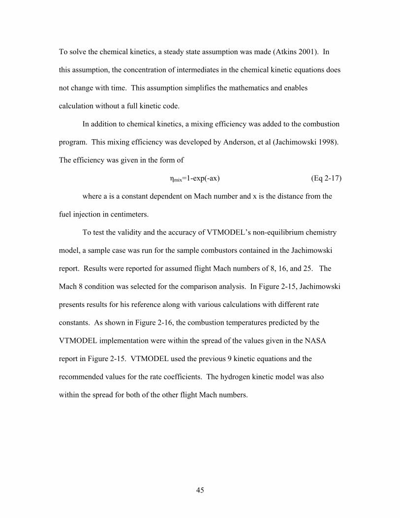
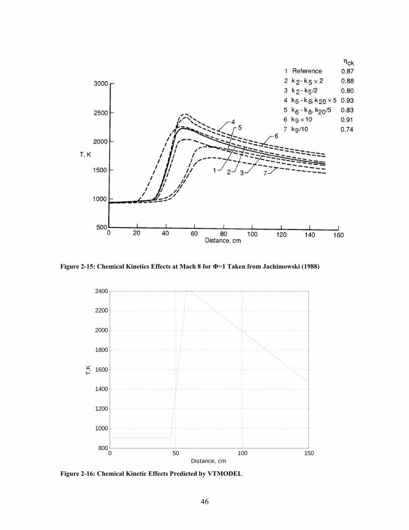
To test the validity and the accuracy of VTMODEL’s non-equilibrium chemistry

model, a sample case was run for the sample combustors contained in the Jachimowski

report. Results were reported for assumed flight Mach numbers of 8, 16, and 25. The

Mach 8 condition was selected for the comparison analysis. In Figure 2-15, Jachimowski

presents results for his reference along with various calculations with different rate

constants. As shown in Figure 2-16, the combustion temperatures predicted by the

VTMODEL implementation were within the spread of the values given in the NASA

report in Figure 2-15. VTMODEL used the previous 9 kinetic equations and the

recommended values for the rate coefficients. The hydrogen kinetic model was also

within the spread for both of the other flight Mach numbers.

46

Figure 2-15: Chemical Kinetics Effects at Mach 8 for Φ=1 Taken from Jachimowski (1988)

Figure 2-16: Chemical Kinetic Effects Predicted by VTMODEL

0 50 100 150800

1000

1200

1400

1600

1800

2000

2200

2400

Distance, cm

T,K

47

2.3.3. Comparison of Combustion Temperatures Produced by the

Complete Combustion Chemistry Model vs. Non-Equilibrium

Chemistry Model

As previously shown, the compete combustion (equilibrium) and non-equilibrium

models of VTMODEL can both be used to calculate combustion temperatures. A

comparison of the results of the two models for a given pressure profile input is shown in

Figure 2-18. The combustor pressure profile was obtained from University of Virginia’s

direct connect tunnel (Rockwell 2010).

Figure 2-17: Comparison of Non Equilibrium and Equilibrium Chemistry Models

0 0.05 0.1 0.15 0.2 0.25 0.3 0.351000

1050

1100

1150

1200

1250

1300

1350

1400

1450

Combustor Length (m)

Sta

tic T

empe

ratu

re (

K)

Equilibrium Model

Non Equilibrium Model

48

As can be seen in Figure 2-17, the two combustion models predict different static

temperature distributions. The differences in slope can be attributed to the difference in

the kinetic mixing parameters and the fuel-air combustion product sphere assumptions.

49

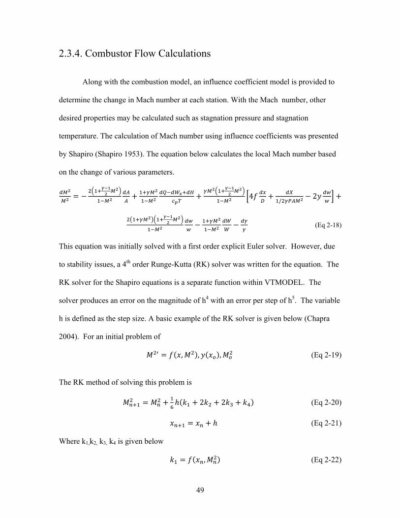
2.3.4. Combustor Flow Calculations

Along with the combustion model, an influence coefficient model is provided to

determine the change in Mach number at each station. With the Mach number, other

desired properties may be calculated such as stagnation pressure and stagnation

temperature. The calculation of Mach number using influence coefficients was presented

by Shapiro (Shapiro 1953). The equation below calculates the local Mach number based

on the change of various parameters.

4/

2

(Eq 2-18)

This equation was initially solved with a first order explicit Euler solver. However, due

to stability issues, a 4th order Runge-Kutta (RK) solver was written for the equation. The

RK solver for the Shapiro equations is a separate function within VTMODEL. The

solver produces an error on the magnitude of h4 with an error per step of h5. The variable

h is defined as the step size. A basic example of the RK solver is given below (Chapra

2004). For an initial problem of

, , , (Eq 2-19)

The RK method of solving this problem is

2 2 (Eq 2-20)

(Eq 2-21)

Where k1,k2, k3, k4 is given below

, (Eq 2-22)

50

, (Eq 2-23)

, (Eq 2-24)

, (Eq 2-25)

The default step size h was determined using an informal initial sensitivity

analysis. The step size of h=0.001 was selected as the initial step size for any combustor

below 1 meter in length. An initial step size of 0.01 was selected for any combustor

above 1 meter in length. The flow equations are solved with decreasing step size until

there is no significant change in the results between the step sizes. The solver

automatically decreases the step size to obtain a result independent of h.

From Equation 2-18, there are multiple parameters that effect the calculation of

the local Mach number. The program defaults some of these values to zero. These

values are the change in body force and change in work. For friction coefficient, a value

of 0.0015 is set as the default. The value can be changed by the user.

Basic heat transfer is included in the program as an option to calculate the cooling

load and the heat transfer in the combustor. The calculation uses Reynolds Analogy to

calculate the heat transfer. The skin friction Cf can be calculated by Equation 2-26 or if

known can be entered in as a parameter for Equation 2-27.

/ (Eq 2-26)

(Eq 2-27)

From this relationship, the Stanton number can be used to calculate h using Equation 2-

28.

(Eq 2-28)

51

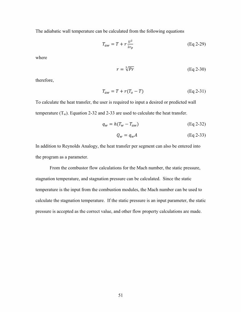
The adiabatic wall temperature can be calculated from the following equations

(Eq 2-29)

where

√ (Eq 2-30)

therefore,

(Eq 2-31)

To calculate the heat transfer, the user is required to input a desired or predicted wall

temperature (Tw). Equation 2-32 and 2-33 are used to calculate the heat transfer.

(Eq 2-32)

(Eq 2-33)

In addition to Reynolds Analogy, the heat transfer per segment can also be entered into

the program as a parameter.

From the combustor flow calculations for the Mach number, the static pressure,

stagnation temperature, and stagnation pressure can be calculated. Since the static

temperature is the input from the combustion modules, the Mach number can be used to

calculate the stagnation temperature. If the static pressure is an input parameter, the static

pressure is accepted as the correct value, and other flow property calculations are made.

52

2.3.5. Use of Other Combustion Models and Fuels

In addition to the two implemented combustion models, VTMODEL is written so

that other combustion models can be integrated into the program. One of the expansions

that are being planned is a hydrocarbon combustion module for predictions of flow

properties for a hydrocarbon scramjet combustion test rig being developed at Virginia

Tech. Providing the ability to use different kinetic and equilibrium chemistries models

was one of the major goals in developing VTMODEL.

53

2.4 Nozzle Modeling

The nozzle module is an optional component of VTMODEL. For analyses with

data from a direct connect tunnel like the University of Virginia Facility, the nozzle

module is bypassed and not used. However, the module can be added for flight

experiments, or full engine wind tunnel experiments. With the nozzle module, the

scramjet performance is calculated using a defined nozzle adiabatic efficiency.

(Eq 2-34)

Using the efficiency, the exit Mach number and other performance variables are

calculated from following equations. Note that the nozzle exit pressure is a required

input for the calculation.

(Eq 2-35)

ϒ (Eq 2-36)

(Eq 2-37)

(Eq 2-38)

(Eq 2-39)

54

Chapter 3

Summary of Model Features and Operations

VTMODEL is written in MATLAB® as a series of functions. The user inputs

required for the full flow path program are the geometry of the flow path, flight Mach

number and altitude, combustion efficiency, equivalence ratio, combustion entrance

pressure, and combustion or nozzle exit pressure. The user also has the ability to enter in

a static pressure distribution for the flow path in the event of a combustion tunnel test

validation.

For design or predictive usage, one of the following components must be

determined either by estimation or by previous experiments. These components are the

combustion entrance pressure, combustion exit pressure or nozzle exit pressure. Once the

pressure at one of these points is set as an anchor point, VTMODEL will iterate upon a

solution to match this point. When the combustion entrance pressure is set, the

combustor and nozzle portions will only be run once, while the isolator shock length or

shock angles will be adjusted to match this pressure. When either the combustor exit

pressure or the nozzle exit pressure is selected as the anchor point, the isolator shock

length or shock angles will be iterated to obtain a matching combustion pressure entrance

state.

55

The full program flow path is given below.

Figure 3-1: Overall Flow Chart for VTMODEL

As shown on the flow path, the isolator module is modified in each loop to match

a combustion exit pressure or another pressure anchor point. The detail of the

combustion program is shown in Figure 3-2. This figure shows the process for each

calculation interval in the program. The process is repeated until the end of the

combustor. This calculation interval is decreased in each iteration until the changes in

predicted temperatures are less than 1%. This assures that the result is not dependent on

the step size of the solver.

56

Figure 3-2: Flow Chart of Combustion Modeling for VTMODEL

One of the benefits of VTMODEL is the ability to separate an analysis into

components. A beneficial use of this separation would be the analyses of direct connect

conditions. Since the isolator entrance condition is generally known, the flow conditions

including the local pressure can be entered directly into the model. The nozzle can also be

included or ignored for the calculation. For an analytical model of experimental results,

VTMODEL is flexible enough to use user input static pressures at any location.

Results of VTMODEL analyses can be saved individually for each run. Since all

of the analysis and predictive tools are separate functions, the main program can be

modified for each run, and geometries entries need not be repeated. Each of the functions

57

in VTMODEL has a description of the variables necessary for the function to run and

output the results data correctly. The general format for calling up a function is [variables

output separated by commas]=function name (inputted variables separated by commas).

The individual function can be called up independent of the rest of the program. For

instance, to examine just the flow in an isolator, only the isolator function has to be called

up.

VTMODEL can be segmented to allow the user to use only the functions that are

necessary to solve their problem. The way VTMODEL is written allows the user to

calculate and account for shock trains in the isolator that can be caused by the

combustion system. The user can also see thermodynamic data at every axial position

within the combustor. The code is written so that only the inlet, shock train isolator, and

nozzle are calculated by the entrance and outlet conditions. The Fanno flow/oblique

shock isolator model has intermediate points where the Fanno flow ends and the area

incorporating the reflected shocks begins. The combustor model is written so that

temperature, stagnation temperature, stagnation pressure, and pressure are calculated at

every segment location across the combustor. Since only the exit pressure for either the

combustor or the nozzle has to be defined downstream, VTMODEL allows modeling of

systems where a full set of data may be not available.

58

Chapter 4

Parameterization of factors with a generic scramjet geometry with VTMODEL

To demonstrate the use of the predictive capabilities of VTMODEL in designing a

scramjet flow path, an example generic model was created. The flow path was specified

with a generic length inlet function with the MIL SPEC inlet pressure recoveries for the

flight Mach numbers. The following parameters were used in the program

Flight Mach numbers were varied between 5 and 10

Altitudes varied between 50,000 to 80,000 ft

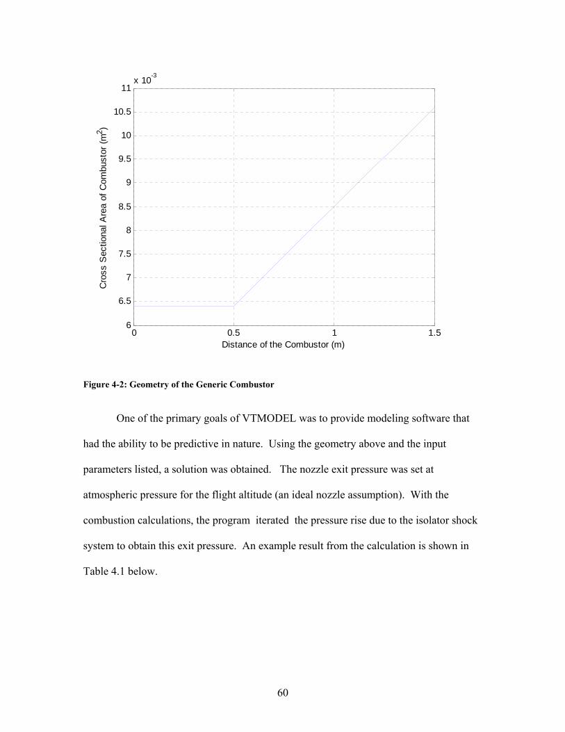
Combustor equivalence ratio was 0.1<Φ<1

Isolator dimensions: width=0.08 m and length=0.8 m

Isolator model: McLafferty rectangular shock train correlation

Combustor length is 1.50 meters

Constant cross sectional area of section of the combustor was 0.50 square

meters

Combustor diverged at an angle of 3% for the remainder of the

combustor length (see Figure 4-2)

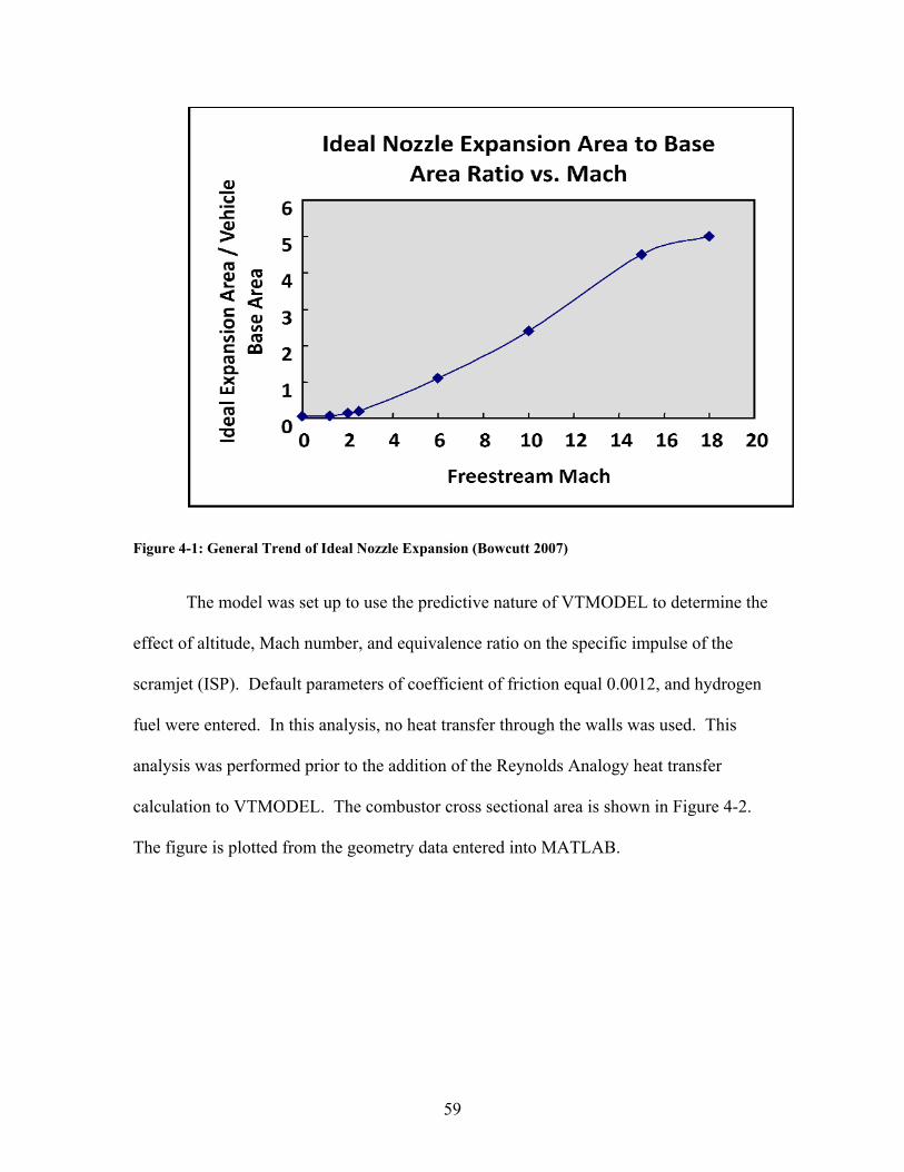
Nozzle parameters were set to have an efficiency of 95% and an area

ratio of 1.5. This area ratio was taken from Figure 4-1 for the

approximate average value between freestream Mach numbers of 5 -10.

59

Figure 4-1: General Trend of Ideal Nozzle Expansion (Bowcutt 2007)

The model was set up to use the predictive nature of VTMODEL to determine the

effect of altitude, Mach number, and equivalence ratio on the specific impulse of the

scramjet (ISP). Default parameters of coefficient of friction equal 0.0012, and hydrogen

fuel were entered. In this analysis, no heat transfer through the walls was used. This

analysis was performed prior to the addition of the Reynolds Analogy heat transfer

calculation to VTMODEL. The combustor cross sectional area is shown in Figure 4-2.

The figure is plotted from the geometry data entered into MATLAB.

60

Figure 4-2: Geometry of the Generic Combustor

One of the primary goals of VTMODEL was to provide modeling software that

had the ability to be predictive in nature. Using the geometry above and the input

parameters listed, a solution was obtained. The nozzle exit pressure was set at

atmospheric pressure for the flight altitude (an ideal nozzle assumption). With the

combustion calculations, the program iterated the pressure rise due to the isolator shock

system to obtain this exit pressure. An example result from the calculation is shown in

Table 4.1 below.

0 0.5 1 1.56

6.5

7

7.5

8

8.5

9

9.5

10

10.5

11x 10

-3

Distance of the Combustor (m)

Cro

ss S

ectio

nal A

rea

of C

ombu

stor

(m

2 )

61

Table 4-1: VTMODEL Results for Φ=1, Mach 7, Altitude=65,000 ft

Figure 4-3: Theoretical ISP for Various Systems (Moses 2003)

Moses (2003) obtained the performance results shown in Figure 4-3. As shown,

the predicted theoretical ISP for a scramjet between flight Mach numbers of 5 and 10 is

between 2000-3500 s. The ISP decreases as Mach number increases. A parameterization

on flight Mach numbers was performed using the above generic VTMODEL, and ISP was

Station P(kPa) T (K) M

a 5.69 216 7

0 5.69 216 7

1 23.7 325 5.56

2 103.6 319 5.62

3 49.8 2015 3.84

4 5.69 1392 5.63

62

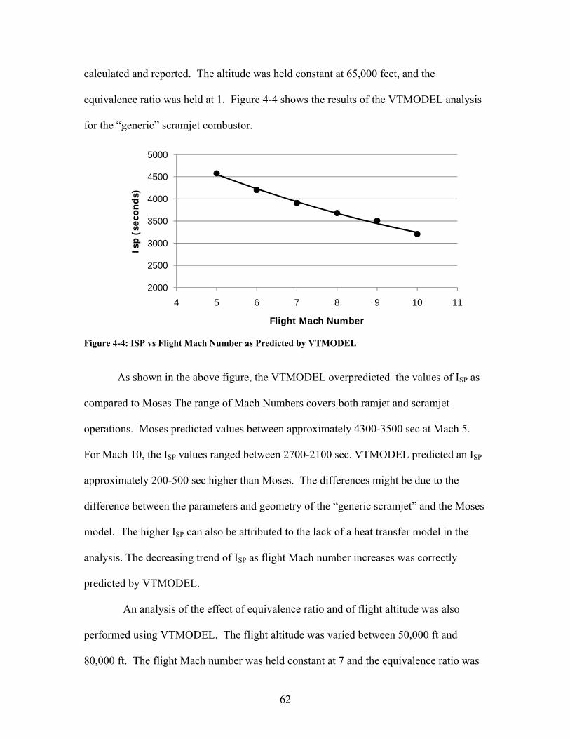
calculated and reported. The altitude was held constant at 65,000 feet, and the

equivalence ratio was held at 1. Figure 4-4 shows the results of the VTMODEL analysis

for the “generic” scramjet combustor.

Figure 4-4: ISP vs Flight Mach Number as Predicted by VTMODEL

As shown in the above figure, the VTMODEL overpredicted the values of ISP as

compared to Moses The range of Mach Numbers covers both ramjet and scramjet

operations. Moses predicted values between approximately 4300-3500 sec at Mach 5.

For Mach 10, the ISP values ranged between 2700-2100 sec. VTMODEL predicted an ISP

approximately 200-500 sec higher than Moses. The differences might be due to the

difference between the parameters and geometry of the “generic scramjet” and the Moses

model. The higher ISP can also be attributed to the lack of a heat transfer model in the

analysis. The decreasing trend of ISP as flight Mach number increases was correctly

predicted by VTMODEL.

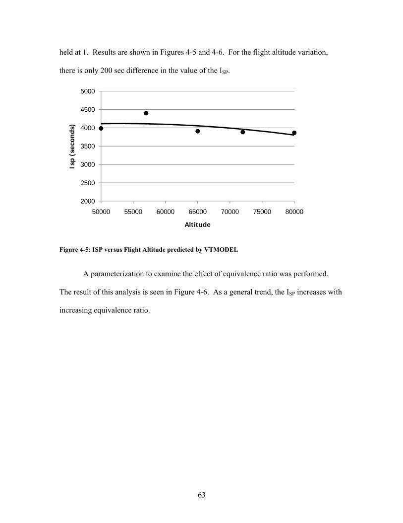
An analysis of the effect of equivalence ratio and of flight altitude was also

performed using VTMODEL. The flight altitude was varied between 50,000 ft and

80,000 ft. The flight Mach number was held constant at 7 and the equivalence ratio was

2000

2500

3000

3500

4000

4500

5000

4 5 6 7 8 9 10 11

Isp

(sec

onds

)

Flight Mach Number

63

held at 1. Results are shown in Figures 4-5 and 4-6. For the flight altitude variation,

there is only 200 sec difference in the value of the ISP.

Figure 4-5: ISP versus Flight Altitude predicted by VTMODEL

A parameterization to examine the effect of equivalence ratio was performed.

The result of this analysis is seen in Figure 4-6. As a general trend, the ISP increases with

increasing equivalence ratio.

2000

2500

3000

3500

4000

4500

5000

50000 55000 60000 65000 70000 75000 80000

Isp

(sec

onds

)

Altitude

64

Figure 4-6: ISP versus Equivalence Ratio as predicted by VTMODEL

From the above analysis, VTMODEL is shown to be a predictive tool for engine

cycle analysis of a ramjet or a scramjet engine. In the simulations presented, the internal

flow data produced by VTMODEL showed that at Mach 5, with an equivalence ratio of

1, the engine was functioning as a ramjet, with subsonic combustion. At Mach 10, the

combustion was supersonic. Even though only the Isp value is graphed and compared to

Moses for the generic scramjet combustor, a full thermodynamic data set was calculated

by VTMODEL for each case.

2000

2500

3000

3500

4000

4500

5000

0 0.2 0.4 0.6 0.8 1

Isp

(sec

onds

)

Equivalance Ratio

65

Chapter 5

Comparison of Results with Other Models and Experimental Data

5.1 Comparison with Results of Other Models

To further demonstrate the validity of VTMODEL as a viable option for scramjet

and ramjet analysis, VTMODEL was run with various geometries to compare to other

published models. The comparisons were based on the primary sources and published

materials. The two main comparisons for predictive modeling were taken from the

doctorate dissertations of Bradford (Bradford 2001) and Bonanos (Bonanos 2005). The

experimental data was taken from the University of Virginia wind tunnel (Rockwell

2010).

5.1.1. SCCREAM

SCCREAM was developed at Georgia Tech in Atlanta, Georgia as part of a

Rocket Combined Cycle Analysis program (Bradford 2001). SCCREAM is the scramjet

analysis section of the program. SCCREAM uses an equilibrium solver for hydrogen

combustion. The following analysis was taken from the doctoral dissertation by Bradford

as part of his comparison of SCCREAM to RJPA. The combustor geometry that he used

is given below in Figure 5-1. Note that the geometry is different from the VTMODEL

standard generic geometry that was given in Chapter 4.

66

Figure 5-1: SCCREAM Combustor Geometry (Bradford 2001)

As can be seen from the Figure 5-1, the combustor is constantly diverging with a

change in slope at x/L= 0.55. The portion of the combustion for 0<x/L<0.55 is taken as

the isolator in the system. The portion for 0.55<x/L<1.0 is assumed to be the region of

the combustion reaction. Since this geometry was different from the default VTMODEL

geometry, to compare results the VTMODEL combustor and isolator geometry were

modified to provide an area change. The area change in the beginning of the combustor

(prior to the reaction region) was modeled using the RK solver to solve for the change in

Mach number due to flow with only friction and change in area (no combustion). This

region was then followed by the reflected oblique shock function at the end of the

isolator. The “reaction region” was modeled to be the combustor in VTMODEL. In

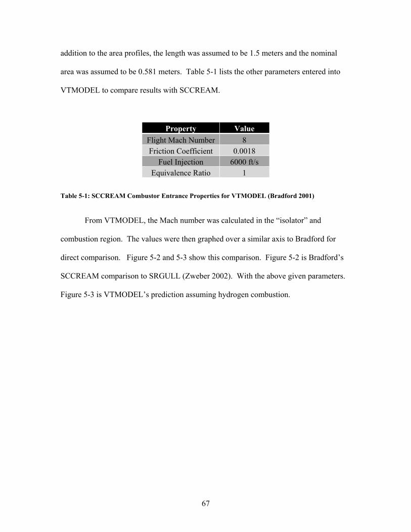
67

addition to the area profiles, the length was assumed to be 1.5 meters and the nominal

area was assumed to be 0.581 meters. Table 5-1 lists the other parameters entered into

VTMODEL to compare results with SCCREAM.

Property Value

Flight Mach Number 8 Friction Coefficient 0.0018

Fuel Injection 6000 ft/s Equivalence Ratio 1

Table 5-1: SCCREAM Combustor Entrance Properties for VTMODEL (Bradford 2001)

From VTMODEL, the Mach number was calculated in the “isolator” and

combustion region. The values were then graphed over a similar axis to Bradford for

direct comparison. Figure 5-2 and 5-3 show this comparison. Figure 5-2 is Bradford’s

SCCREAM comparison to SRGULL (Zweber 2002). With the above given parameters.

Figure 5-3 is VTMODEL’s prediction assuming hydrogen combustion.

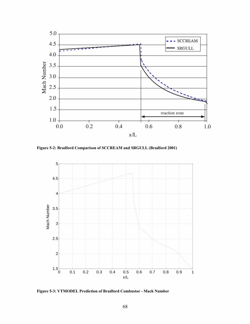
68

Figure 5-2: Bradford Comparison of SCCREAM and SRGULL (Bradford 2001)

Figure 5-3: VTMODEL Prediction of Bradford Combustor - Mach Number

0 0.1 0.2 0.3 0.4 0.5 0.6 0.7 0.8 0.9 11.5

2

2.5

3

3.5

4

4.5

5

x/L

Mac

h N

umbe

r

69

VTMODEL predicted the Mach number decrease in the combustor to be of the

same order of magnitude as Bradford’s calculations. The other thermodynamic values

such as combustion temperature were not included in his dissertation, so the VTMODEL

results are not included for comparison.

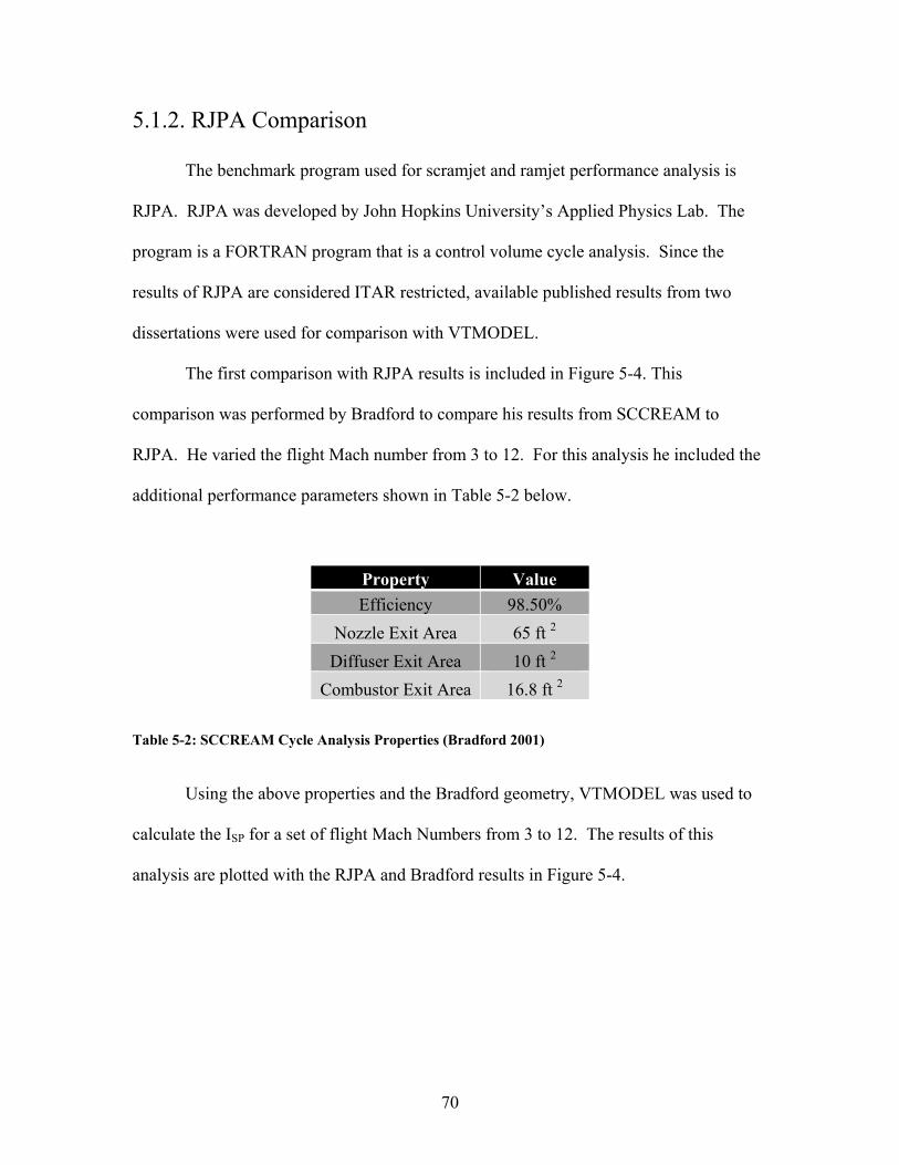
70

5.1.2. RJPA Comparison

The benchmark program used for scramjet and ramjet performance analysis is

RJPA. RJPA was developed by John Hopkins University’s Applied Physics Lab. The

program is a FORTRAN program that is a control volume cycle analysis. Since the

results of RJPA are considered ITAR restricted, available published results from two

dissertations were used for comparison with VTMODEL.

The first comparison with RJPA results is included in Figure 5-4. This

comparison was performed by Bradford to compare his results from SCCREAM to

RJPA. He varied the flight Mach number from 3 to 12. For this analysis he included the

additional performance parameters shown in Table 5-2 below.

Property Value

Efficiency 98.50%

Nozzle Exit Area 65 ft 2

Diffuser Exit Area 10 ft 2

Combustor Exit Area 16.8 ft 2

Table 5-2: SCCREAM Cycle Analysis Properties (Bradford 2001)

Using the above properties and the Bradford geometry, VTMODEL was used to

calculate the ISP for a set of flight Mach Numbers from 3 to 12. The results of this

analysis are plotted with the RJPA and Bradford results in Figure 5-4.

71

Figure 5-4: ISP vs Mach number as Predicted by SSCREAM, RJPA (Bradford 2001), and VTMODEL

Comparing the results, it can be seen that as for the comparisons with the results

of Moses in Chapter 4, VTMODEL also consistently overpredicts ISP with respect to

SCCR EAM and RJPA. There are many possible reasons for this over prediction. In his

analysis, Bradford stated that he adjusted the equivalence ratio to suit the fuel flow rate

from RJPA. The VTMODEL analysis assumed an equivalence ratio of 1. In addition,

since heat transfer through the walls was neglected, the calculated ISP will be higher.

VTMODEL also does not allow the user to specify ramjet or scramjet mode. The model

automatically calculates the combustor entrance parameter based on the other parameters

used. Therefore, at Mach 6, there is only one ISP value calculated for VTMODEL.

Given the above results, another comparison of VTMODEL to RJPA was desired.

Bonanos used RJPA to perform cycle analysis and combustion efficiency analysis on

experimental data obtained from the University of Virginia wind tunnel. He compared

72

his results with an “aeroramp” injector and flame holder to those for a physical ramp.

Since Bonanos used air specific impulse as a performance factor, the nozzle function of

VTMODEL was modified to include this additional calculation. Air specific impulse is

calculated by the following equation:

(Eq 5-1)

In addition, the geometry and entrance conditions for VTMODEL were modified

to allow for comparison. The combustor parameters used for the VTMODEL

comparison with Bonanos’ RJPA results are given below in Table 5-3.

Properties Values

Combustor Length 0.23 m Combustor Entrance

Area 9.6e-4 m2

Combustor Exit Area 1.2e-3 m2 Friction Coefficient 0.0023 Nozzle Efficiency 98.50%

Table 5-3: RJPA and VTMODEL Cycle Analysis Properties (Bonanos 2005)

In addition to the cycle analysis properties presented in Table 5-3, Bonanos used

Reynolds Analogy to calculate heat transfer through the walls for each one of his

experimental cases. The results of this analysis were included in the VTMODEL ISP

calculations. Bonanos desired a comparison between performance with ethylene and

hydrogen fuels, so he normalized his results based on the following expression:

∗ / ∗

The results of analysis are shown in Figure 5-5. He shows the variation of Air Specific

Impulse for the ramp and aeroramp geometry tested in the UVA wind tunnel.

73

Figure 5-5: Air Specific Impulse from RJPA (Bonanos 2005)

Bonanos also wanted to see the effect of combustor inlet total temperature on air specific

impulse. He set up the following parameters for the case of To=1010K.

530<To(K)<1010

Flight Mo=4.22

Altitude=88000 ft

Inlet Area= 9.65 in2

Area Ratio=6.43

For this set of data, he was able to calculate the results shown in Figure 5-6.

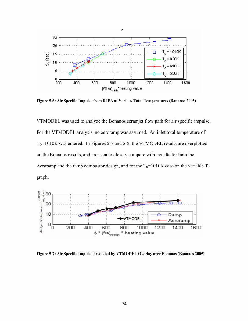
74

Figure 5-6: Air Specific Impulse from RJPA at Various Total Temperatures (Bonanos 2005)

VTMODEL was used to analyze the Bonanos scramjet flow path for air specific impulse.

For the VTMODEL analysis, no aeroramp was assumed. An inlet total temperature of

TO=1010K was entered. In Figures 5-7 and 5-8, the VTMODEL results are overplotted

on the Bonanos results, and are seen to closely compare with results for both the

Aeroramp and the ramp combustor design, and for the T0=1010K case on the variable T0

graph.

Figure 5-7: Air Specific Impulse Predicted by VTMODEL Overlay over Bonanos (Bonanos 2005)

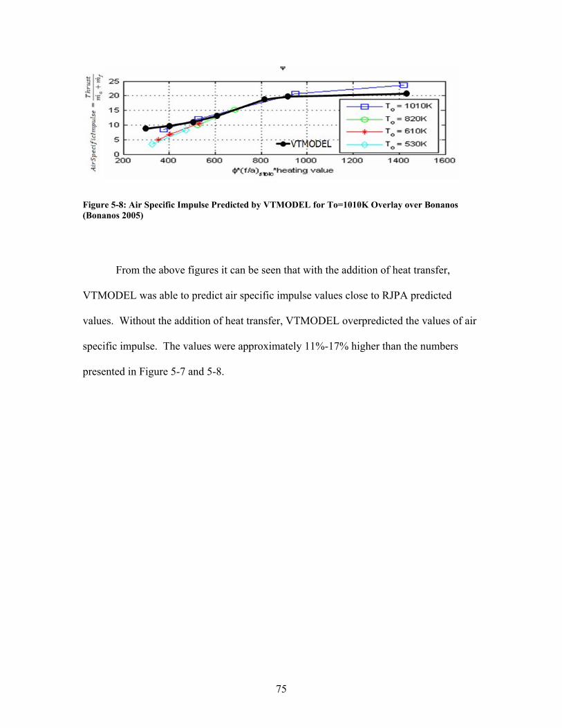
75

Figure 5-8: Air Specific Impulse Predicted by VTMODEL for To=1010K Overlay over Bonanos (Bonanos 2005)

From the above figures it can be seen that with the addition of heat transfer,

VTMODEL was able to predict air specific impulse values close to RJPA predicted

values. Without the addition of heat transfer, VTMODEL overpredicted the values of air

specific impulse. The values were approximately 11%-17% higher than the numbers

presented in Figure 5-7 and 5-8.

76

5.2 Comparisons with Experimental Data 5.1.1. Analysis of UVA Experimental Results

VTMODEL was used to compare to results from the University of Virginia Direct

Connect Combustion Tunnel. Operating conditions for the tunnel were as shown in

Table 5.4. The geometry of the tunnel is as shown in Figure 5-9. The tunnel was set up

to simulate Mach 5, 70,000 ft flight. The isolator entrance conditions were as shown in

Table 5-4 for clean air. The equivalence ratio analyzed was 0.341.

Table 5-4: UVA Isolator Entrance Parameters (Rockwell 2010)

77

Figure 5-9: Schematic of UVA Tunnel (Le 2008)

A predictive analysis using VTMODEL was run for this case. The only modules

used in this analysis are the Isolator and Combustor. The isolator geometry was fixed

based on the schematic of the UVA tunnel. The incoming properties were taken from

Table 5-4. The friction coefficient was assumed to be 0.0015 and the Fanno flow and

oblique shock model was used for the isolator. The combustor static pressure anchor

point was set at 0.25 m upstream of the fuel injector. This anchor point was chosen due

to the artifact at the end of the combustor where the static pressure increases. The data set

was assumed to be for subsonic combustion. The Mach number entering the combustor

from the isolator is predicted to be 0.858 by VTMODEL. The flow path Mach number

was reduced to this subsonic value in the isolator. The results of the analysis are shown

in the following figures. The predicted static pressure profiles agree within 5% of the

78

experimental data. The agreement obtained for the pressure profile supports the subsonic

combustor entry Mach number assumption.

In the following figures, the distance from the fuel injectors is given in meters.

Figure 5-10: Static Pressure Predicted by VTMODEL for Φ=0.341 Compared to UVA Experimental Data

0 0.05 0.1 0.15 0.2 0.25 0.3 0.35 0.490

100

110

120

130

140

150

160

170

Distance from Fuel Injector

Sta

tic P

ress

ure

(kP

a)

UVA Experimental Data

VTMODEL Predicted

79

Figure 5-11: Static Temperature Predicted by VTMODEL for Φ=0.341

Figure 5-12: Mach Number Predicted by VTMODEL for Φ=0.341

0 0.05 0.1 0.15 0.2 0.25 0.3 0.35 0.41050

1100

1150

1200

1250

1300

1350


Sta

tic T

empe

ratu

re (K

elvi

n)

0 0.05 0.1 0.15 0.2 0.25 0.3 0.35 0.40.858

0.859

0.86

0.861

0.862

0.863

0.864

0.865

0.866


Mac

h N

umbe

r

80

Figure 5-13: Stagnation Temperature Predicted by VTMODEL for Φ=0.341

0 0.05 0.1 0.15 0.2 0.25 0.3 0.35 0.41200

1250

1300

1350

1400

1450

1500


Sta

gnat

ion

Tem

pera

ture

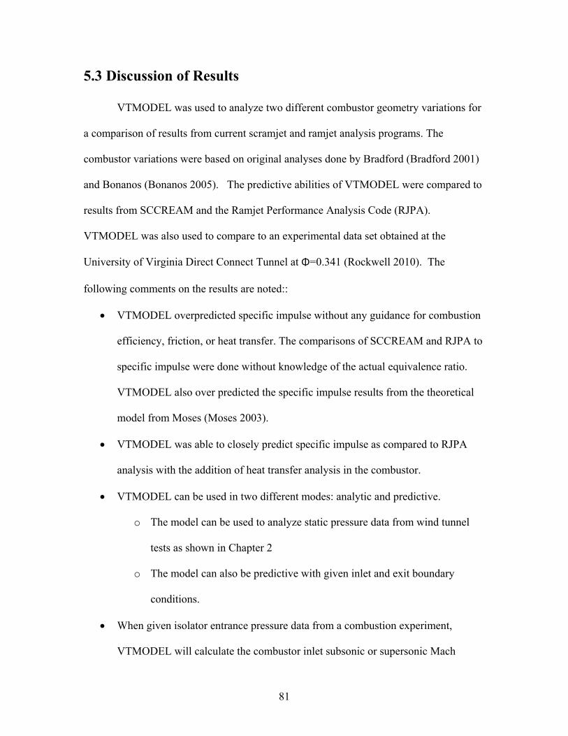
81

5.3 Discussion of Results VTMODEL was used to analyze two different combustor geometry variations for

a comparison of results from current scramjet and ramjet analysis programs. The

combustor variations were based on original analyses done by Bradford (Bradford 2001)

and Bonanos (Bonanos 2005). The predictive abilities of VTMODEL were compared to

results from SCCREAM and the Ramjet Performance Analysis Code (RJPA).

VTMODEL was also used to compare to an experimental data set obtained at the

University of Virginia Direct Connect Tunnel at Φ=0.341 (Rockwell 2010). The

following comments on the results are noted::

VTMODEL overpredicted specific impulse without any guidance for combustion

efficiency, friction, or heat transfer. The comparisons of SCCREAM and RJPA to

specific impulse were done without knowledge of the actual equivalence ratio.

VTMODEL also over predicted the specific impulse results from the theoretical

model from Moses (Moses 2003).

VTMODEL was able to closely predict specific impulse as compared to RJPA

analysis with the addition of heat transfer analysis in the combustor.

VTMODEL can be used in two different modes: analytic and predictive.

o The model can be used to analyze static pressure data from wind tunnel

tests as shown in Chapter 2

o The model can also be predictive with given inlet and exit boundary

conditions.

When given isolator entrance pressure data from a combustion experiment,

VTMODEL will calculate the combustor inlet subsonic or supersonic Mach

82

number required to satisfy the static pressure value at the combustor outlet or at

the nozzle outlet. No assumption is needed regarding the subsonic or supersonic

condition at the combustor inlet. The model will iterate on the shock length in the

combustor to determine the isolator discharge Mach number for the given

pressures.

83

Chapter 6

Conclusions and Recommendations

6.1 Conclusions

An one dimensional scramjet and ramjet analysis code called VTMODEL was

written in MATLAB. VTMODEL was created to be a modular code that can be improved

upon and expanded. The code was constructed with four main sections: the inlet,

isolator, combustor, and nozzle. For the isolator section, the user has a choice of two

different isolator flow models. One of the models is a Fanno flow/ oblique shock system

combination that iterates on the shock angles of the shock system to match an exit

pressure. The second model is a shock train correlation. This correlation iterates on the

shock length to match the exit pressure of the combustor or the nozzle depending on the

system.

Of the four sections of VTMODEL, the combustor is the most involved and

complicated. The complete combustion model includes three functions: a

mixing/combustion efficiency function, a combustion calculation function, and a flow

properties calculation function. The mixing/combustion efficiency function can either be

an efficiency correlation including with the mixing efficiency of the fuel-air mixture, or

a “combustion sphere” model that permits the adjustment of the flame speed of the

combustion, resulting in a prediction of combustion efficiency. The combustion

functions can either a complete combustion model, or a non equilibrium mechanism

specifically for hydrogen combustion. For the complete combustion method, the

concentration of fuel and combustion products in each section of the combustor is

84

determined by the combustion sphere model. The non-equilibrium function uses the

mixing correlation and also a reduced hydrogen combustion chemistry model presented

in Jachimowski (Jachimowski 1988). This reduced hydrogen combustion model is made

up of a system of 8 reactions. The model uses some assumptions of steady state

intermediates to make calculations possible without an additional chemical kinetics code

(Atkins 2001). The third function in the VTMODEL combustor model is a Mach number

calculation using influence coefficients as presented in Shapiro (Shapiro 1953). The

solver for this differential equation was written in MATLAB, and is a 4th order RK

solver. From these three modules, all of the thermodynamic properties at each combustor

section can be calculated.

To illustrate the predictive capability of VTMODEL, the program was used to

analyze a “generic” scramjet flow path. This example was developed to show the cycle

analysis capabilities of VTMODEL. The flow path was analyzed for varying flight

altitudes, Mach numbers, and equivalence ratios. The specific impulse was calculated for

each of these runs. It was determined that VTMODEL correctly predicted the trends of

the ISP vs flight Mach number. The predicted value of the ISP was 200-500 seconds

higher than the “theoretical” values presented in Moses (Moses 2003). Among the many

factors that could influence the predications, the discrepancy could be due to the

assumption of 100% combustion efficiency in VTMODEL, increasing the specific

impulse. The increase could also be due to having no heat transfer through the walls.

VTMODEL was created to be able to analyze and predict thermodynamic data in

both scramjet and ramjet flow paths. To demonstrate use in experiment analysis,

VTMODEL was used to predict thermodynamic data based on an experimental data

85

series furnished by the University of Virginia. The results of this analysis showed that

VTMODEL had the ability to predict temperatures and Mach number along the

combustor. The required inputs were an isolator entrance condition, geometry,

equivalence ratio, and static pressure profiles.

VTMODEL also has a predictive capability. The predictive ability of

VTMODEL was tested against the models RJPA and SCCREAM. VTMODEL predicted

fuel specific impulse and air specific impulse to match the analyses done in Bradford and

Bonanos. The results show that the values predicted by VTMODEL were within 5% of

the values taken from their results. The predictive model capability of VTMODEL was

also shown in one test using data from the University of Virginia Direct Connect

combustor. For an equivalence ratio where the static pressure profile was already

experimentally obtained, VTMODEL was used to predict this profile and also the Mach

numbers, static temperatures, and stagnation temperatures along the combustor. The

results show that VTMODEL was able to predict this profile with a high degree of

accuracy.

VTMODEL currently continues in development as a function based/modular

program to analyze one dimensional flow through a scramjet or ramjet. The benefits of

VTMODEL include an ability to predict flow conditions, or to enter known data for

analysis. Modules of the code can be removed or modified to the user’s specification.

There are limitations to the use of VTMODEL. The most inherent limitation is

the use of a one-dimensional model to model 3D flow. The model also does not take into

account boundary layer effects or separation. The inlet function of the model is a

simplistic model of an actual scramjet inlet. The inlet performance and pressure recovery

86

is most likely somewhere in-between the supplied kinetic energy model and the MIL

Spec model presented in Chapter 2.

Another limitation to VTMODEL is the singularity due to the influence

coefficient calculation for Mach number in the combustor. Since the quantity (1-M2) is in

the denominator, the program currently will not calculate flow through M=1.

VTMODEL is therefore currently useful for modeling subsonic or supersonic combustion

and not for dual mode predictions. This ability for the Mach number to transition from a

supersonic to subsonic value in the combustor is essential for dual mode combustion

calculations.

87

6.2 Recommendations

Several improvements can be made the improve VTMODEL. The program is

currently written in a manner that requires programming knowledge to run the program.

A visual graphical interface can be developed to make the program more user friendly.

The program also is currently in open MATLAB files. The program can be further

refined to allow easier data entry and function call-up. One of the first improvements for

VTMODEL should be to use l’Hopital’s rule or another mathematical technique to be

able to calculate through the M=1 condition. Currently, there is a singularity in the

program at this Mach number due to the influence coefficient method of solving for

Mach number in the combustor. Heat transfer analysis is extremely important for ramjet

and scramjet design and analysis. The current heat transfer analysis model uses Reynolds

Analogy. This heat transfer analysis can be expanded on and improved.

Another improvement for VTMODEL can be the integration of a chemical kinetic

program such as Chemkin. With the development of the complete combustion model

with the combustion sphere combustion delay mechanism, and the uses of the

Jachimowski method for hydrogen, the program will run with rate-controlled combustion

under certain specifications of Mach number and pressures. With the addition of

Chemkin, the development of VTMODEL into a multi fuel code would be quicker and

more accurate. The addition of hydrocarbon fuel capability will also aid in the

development of a comprehensive scramjet and ramjet analysis code.

Currently, there is an Aerojet-sponsored senior design team at Virginia Tech that

is designing and manufacturing a hydrocarbon scramjet test rig for test at the Aerojet

facility in Orange, VA. Since the team is designing for hydrocarbon fuel, there was no

88

benefit in using the current VTMODEL for analysis and for aiding the design. However,

with the development of a hydrocarbon chemistry solver, VTMODEL can be used as

both a design tool and an analysis tool for hydrocarbon combustion testing.

One advantage of VTMODEL is the modular design. Coding VTMODEL in

MATLAB can help expand VTMODEL into a combined cycle code. Since VTMODEL

is already modular, different components of the model can be used to prove the

scramjet/ramjet flow path analysis of a combined cycle code. A combined cycle code

development will enable the model to both analyze scramjet and ramjet flowpaths and

combine these flowpaths with either turbomachinery or rockets. This addition of

combined cycle analysis will enable VTMODEL to aid in the design and analysis of a

system that span sea level to flight altitude analysis.

89

REFERENCES

1. Atkins , P. and dePaula, J. (2001). Physical Chemistry. 7th Ed. New York, W.H

Freeman.

2. Boeing (2010, May 26, 2010). "Boeing X-51A WaveRider Breaks Record in 1st

Flight." 2010, from http://boeing.mediaroom.com/index.php?s=43&item=1227.

3. Bonanos, A. M. (2005). Scramjet Operability Range Studies of an Integrated

Aerodynamic- Ramp-Injector/Plasma-Torch Igniter with Hydrogen and

Hydrocarbon Fuels. Aerospace Engineering. Blacksburg, Virginia Polytechnic

Institute and State University. Doctor of Philosophy.

4. Bowcutt, K. G. (2007). Scramjet Vehicle Propulsion-Airframe Integration.

Hypersonic Propulsion Education Initiative, NIA.

5. Bradford, J. E. (2001). A Technique for Rapid Prediction of Aftbody Nozzle

Performance for Hypersonic Launch Vehicle Design. Aerospace Engineering.

Atlanta, Georgia Institute of Technology. Doctor of Philosophy.

6. Bradford, J. E. and Olds, J.R. (1998). Improvements and Enhancements to

SCCREAM, A Conceptual RBCC Engine Analysis Tool. 34th

AIAA/ASME/SAE/ASEE Joint Propulsion Conference & Exhibit. Cleveland,

OH, American Institute of Aeronautics and Astronautics.

7. Burkardt, L. A. and Franciscus, L.C. (1990). RAMSCRAM-A Flexible

Ramjet/Scramjet Engine Simulation Program. L. R. Center. Cleveland, NASA.

8. Chapra, S. C. (2004). Applied Numerical Methods with MATLAB for Engineers

90

and Scientists. New York, McGraw Hill.

9. Curran, E.T (2001). “Scramjet Engines: The First Forty Years.” Journal of

Propulsion and Power. 17(6):1138-1148.

10. Glassman, I. (1977). Combustion. New York, Academic Press.

11. Goodall, J. and Miller, J. (2002). Lockheed's SR-71 'Blackbird' Family A-12, F-

12, M-21, D-21, SR-71. Hickley, England, AeroFax-Midland Publishing.

12. Handbook, P. W. MIL-E-5007D

13. Heiser, W. H. and Pratt, D.T, Ed. (1994). Hypersonic Air Breathing Propulsion.

AIAA Education Series. Washington D.C, American Institute of Aeronautics and

Astronautics.

14. Hill, P and Peterson, C. (1975). Mechanics and Thermodynamics of Propulsion

1st Edition. New York, Addison Wesley Longman.

15. Hill, P and Peterson, C. (1992). Mechanics and Thermodynamics of Propulsion

2nd Edition. New York, Addison Wesley Longman.

16. Jachimowski, C. (1988). An Analytical Study of the Hydrogen-Air Reaction

Mechanism with Application to Scramjet Combustion. NASA Langley Research

Center. Hampton.

17. John, James. (1984). Gas Dynamics 2nd Edition. New York, Prentice Hall.

18. Kazmar, R. R. (2005). Airbreathing Hypersonic Propulsion at Pratt & Whitney –

Overview. AIAA/CIRA 13th International Space Planes and Hypersonic Systems

and Technologies.

19. Le, D. B., C.P Goyne, R.H Krauss, and J.C. McDaniel (2008). "Experimental

Study of a Dual-Mode Scramjet Isolator." Journal of Propulsion and Power 25(5):

91

1050-1057.

20. Lee, C, Kundu K., and Acosta W. (1991). Jet-A Reaction Mechanism Sutdy for

Combustion Application. NASA Glenn Research Center. Cleveland.

21. Lockheed Martin (2010). "SR-71 Blackbird." 2010, from

http://www.lockheedmartin.com/aboutus/history/SR71Blackbird.html.

22. Moses, P. L. (2003). X-43C Plans and Status. 12th AIAA International Space

Planes and Hypersonic Systems and Technologies Conference. Norfolk, VA.

23. O'Brien, T. F., Ryan P. Starkey, and Mark J. Lewis (2001). "Quasi-One-

Dimensional High-Speed Engine Model with Finite-Rate Chemistry." Journal of

Propulsion and Power 17(6): 1366-1374.

24. O’Byrne, S. and Cutler, A.D. (2007). “Dual-Pump Coherent Anti-Stokes Raman

Scattering Measurements in a Supersonic Combustor.” AIAA Journal 45(4): 922-

933.

25. Pandolfini, P. P., and Friedman, M.A. (1992). Instructions for using Ramjet

Performance Analysis (RJPA) IBM-PC Version 1.24. Baltimore, John Hopkins

University/Applied Physics Lab.

26. Reaction Design (2010). “Chemkin: Leading Solutions for the Rapid Simulation

of Complex Chemistry,” from

http://www.reactiondesign.com/images/CHEMKIN-BRO_0910.pdf.

27. Rockwell, R. (2009-2010). Experimental Data. Personal Communication

28. Schetz, J. A. (2007). Scramjet Combustors. Hypersonic Propulsion Education

Initiative, NIA.

29. Segal, C. (2009). The Scramjet Engine: Processes and Characteristics. New York,

92

Cambridge University Press.

30. Shapiro, A. H. (1953). The Dynamics and Thermodynamics of Compressible

Fluid Flow in Two Volumes. New York, Ronald Press Company.

31. Sullins, G. and McLafferty . (1992). Experimental Results of Shock Trains in

Rectangular Ducts. AIAA Fourth International Aerospace Planes Conference.

Orlando, FL.

32. Trefny, C. (2010). Personal Communication.

33. United States Government Printing Office (1976). US Standard Atmosphere.

34. UMD (University of Maryland) (2010). "Innovation Hall of Fame: Frederick S.

Billig PhD (1933-2006).” http://www.eng.umd.edu/ihof/inductees/billig.html.

35. USAF, Ed. (2002). SR-71 Flight Manual. Manuals of Flight Series, Government

Reprints Pr.

36. Van Wie, D. M. (2001). Scramjet Inlets. Scramjet Propulsion (Progress in

Astronautics and Aeronautics). P. Zarchan. 189.

37. Waltrup, P. J., and F.S. Billig (1973). "Prediction of Precombustion Wall Pressure

Distributions in Scramjet Engines." Journal of Spacecraft 10(9).

38. Waltrup, P. J., Billig F.S., and Stockbridge, R.D. (1978). A Procedure for

Optimizing the Design of Scramjet Engines. AIAA/SAE 14th Joint Propulsion

Conference. Las Vegas, American Institute of Aeronautics and Astronautics.

39. Waltrup, P.J., White, M., Zarlingo, F. and Gravlin, E. (1997). “History of Ramjet

and Scramjet Propulsion Development for U.S. Navy Missiles.” John Hopkins

APL Technical Digest. 18(2): 234-244.

40. Warwick, G. (2010). First X-51A Hypersonic Flight Deemed Success. Aviation

93

Week.

41. Zweber, J. V., Hanee Kabis, William W. Follett, and Narayan Ramabadran

(2002). Towards an Integrated Modeling Environment for Hypersonic Vehicle

Design and Synthesis. AIAA/AAAF 11th International Space Planes and

Hypersonic Systems and Technologies Conference. New Orleans, American

Institute of Aeronautics and Astronautics.

94

UNCITED REFERENCES

1. Aithal, S. M., V.V. Subramaniam and V. Babu (1996). Numerical simulation of

plasma and reacting flows. 27th AIAA Fluid Dynamics Conference. New

Orleans, LA, American Institute of Aeronautics and Astronautics.

2. Baurle, R. "VULCAN: Viscous Upwind Algorithm for Complex Flow Analysis,

User Manual." from http://vulcan-cfd.larc.nasa.gov/.

3. Billig, F. S., Dugger G.L, Waltrup P.J (1972). Inlet-Combustor Interface

Problems in Scramjet Engines. 1st International Symposium on Air Breathing

Engines. Marseille, France, Institut de Mecanique des Fluides.

4. Bussing, T. R., Murman E.M (1983). A one-dimensional unsteady model of dual

mode scramjet operation. 21st Aerospace Sciences Meeting. Reno, NV, American

Institute of Aeronautics and Astronautics.

5. Clark, A., Chivey Wu, Maj Mirmirani, Sangbum Choi (2006). Development of an

Airframe-Propulsion Integrated Generic

6. Cutler, A.D, Danehy, P.M., Springer, R.R, O’Bryne, S., Capriotti, D.P., and

Deloach, R.” Coherent Anti-Stokes Raman Spectroscopic Thermometry in a

Supersonic Combustor.” AIAA Journal 41(12): 2451-2459.

7. Hypersonic Vehicle Model. 44th AIAA Aerospace Sciences Meeting and Exhibit.

Reno, NV, American Institute of Aeronautics and Astronautics.

8. Doolan, C. (2008). A Quasi-One-Dimensional Mixing and Combustion Code for

Trajectory Optimization and Design Studies. 15th AIAA International Space

Planes and Hypersonic Systems and Technologies Conference. Dayton, Ohio,

95

American Institute of Aeronautics and Astronautics.

9. Kato, R. a. I. K. (1996). Numerical Simulation of Flame-Stabilization and

Combustion Promotion by Plasma Jets in Supersonic Air Streams. Twenty-Sixth

Symposium on Combustion, The Combustion Institute

10. Minato, R., Takashi Niioka, Hiromu Sugiyama, and Kazuhide Mizobata (2005).

Numerical Analysis of Supersonic Combustion by a Plasma Torch. AIAA/CIRA

14th International Space Planes and Hypersonic Systems and Technologies,

American Institute of Aeronautics and Astronautics.

11. Roberts, K. (2008). Analysis and Design of a Hypersonic Scramjet Engine with a

Starting Mach number of 4.00. Aerospace Engineering. Arlington, University of

Texas at Arlington. Master of Science.

12. Ruscic, B., Reinhardt E. Pinzon, Melita L. Morton, Nanda K. Srinivasan, and J.

W. S. a. J. V. M. Meng-Chih Su (2006). "Active Thermochemical Tables:

Accurate Enthalpy of Formation of Hydroperoxyl Radical, HO2." Journal of

Physical Chemistry A 110: 6592-6601.

13. Starkey, R. P. (2004). Scramjet Optimization for Maximum Off-Design

Performance. 40th AIAA/ASME/SAE/ASEE Joint Propulsion Conference and

Exhibit. Fort Lauderdale, Fl, American Institute of Aeronautics and Astronautics.

14. Tomioka, S., Tetsuo Hiraiwa, Kan Kobayashi, Muneo Izumikawa, Tomoyuki

Kishida, and Hiroyuki Yamasaki (2007). "Vitiation Effects on Scramjet Engine

Performance in Mach 6 Flight Conditions." Journal of Propulsion and Power

23(4): 789-796.

15. Turns, S. R. (2000). An Introduction to Combustion: Concepts and Applications.

96

New York, McGraw-Hill Higher Education.

16. Weissman, D. (1990). Representation of two-dimensional hypersonic inlet flows

for one-dimensional scramjet cycle analysis 28th Aerospace Sciences Meeting.

Reno, NV, American Institute of Aeronautics and Astronautics.

one dimensional analysis program for scramjet and …...... using an influence coefficient method....

Documents