on the use of cbir in image mosaic generationzaiane/postscript/thesis/yuezhang... · on the use of...
TRANSCRIPT
On the use of CBIR in Image Mosaic Generation
by
Yue Zhang
Technical Report TR 02-17July 2002
DEPARTMENT OF COMPUTING SCIENCEUniversity of Alberta
Edmonton, Alberta, Canada
On the use of CBIR in Image Mosaic Generation
Yue Zhang
July 29, 2002
Abstract
Image mosaic or image montage is an image made up of many other images. An image mosaic has its ownvisual content as a whole while each of its building images also has a meaningful content. This thesis addressthe design and implementation of an image mosaic generating system, which uses computers to build imagemosaics automatically. There are many parameters used in our system to control an image mosaic generatingprocess which are shown playing different roles on affecting the processing time and image mosaic’s quality.
As another contribution, a new approach used to evaluate an image mosaic’s quality is proposed in thisthesis, which is based on the human perception of image mosaics. It uses the increasing speed of distancebetween local colour histograms of an image mosaic and its original image as the distance measure. And theexperimental results show that this distance measure performs the most stable for evaluating image mosaics’quality in comparison with Global Colour Histogram and Average Pixel-to-Pixel distance measure.
1 Introduction and Motivation
1.1 Introduction of Image Mosaics
Is there a relationship between computer science and the arts? Yes. Using computer technology in differentkinds of art has a long history. Especially nowadays, the emergence of various advanced computer technologiesgives computer art a whole new life. We have seen a broad range of work which is created using computers asmediums or tools. For instance, Echen uses different colours to denote different letters in forming his “Art fromtext” [6]. Marius Hartman explores facial multiplicity by combining different faces generated by a computer atdifferent times in his “10000 zombies” [13]. Many other examples of computer art exist – ranging from digitalmusic composed by computers to virtual cameras used in the 3D world.
Robert Silvers, a former MIT media Lab graduate student, used a computer as a tool to create images withan amazing appearance, called photomosaics [27]. A photomosaic, or an image mosaic, or an image montage –which is also the focus of our thesis – is an image made up of many other images. Each of the building imageshas its own content, and all these building images are put together to generate a single image which also has itsown meaningful content. The visual effect of an image mosaic is that its content, instead of each building image,can only be seen clearly from many steps away.
Using many images to build a single image has a long history. Back in the 16th century, the painter GiuseppeArcimboldo used vegetables, fruit, and flowers as building images to build an image mosaic [37]. Salvador Dalicreated a well known image montage of Abraham Lincoln by putting many other images together including hiswife’s picture, which is shown in Figure 1. Using computers to build image mosaics is a big step in their history.Robert Silvers, as we mentioned, is the inventor of using computer technology to generate image mosaics, andthe patent holder for his image mosaic generating system “Photomosaic” [27].
1

Figure 1: The image montage of Abraham Lincoln [Salvador Dali]
1.2 Image Mosaics and Image Retrieval
In general, an image mosaic is generated based on an original image. The requirement of the image mosaic isthat it retains similar visual content to the original image, while being made up of many images. Most modernimage mosaic generating systems using computer technology contain the following steps:
� Divide the original image into many tiles.
� For each tile, find another image with similar content from an image database.
� Build the image mosaic by replacing all tiles by their similar images.
The second step – selecting an image having similar content with a tile from a large image database – is calledContent-based Image Retrieval (CBIR). CBIR plays an important role in an image mosaic generating system. Thequality of the resulting image mosaic directly depends on the effectiveness of the CBIR technique used in thesystem.
CBIR is currently an active research area in computing science, as more and more visual information –especially digital images – has been made available in digital archives. The basic task of a CBIR system is tofind similar images according to their visual features, within a large image database. Query By Example (QBE)is one of the most popular methodologies used in CBIR systems, in which images are selected from an imagedatabase similar to a given image presented by users. IBM’s QBIC [21] is such a CBIR system.
Typically, a CBIR system pre-processes an image database in order to extract information from all images inthe database. This information is referred to as visual features of images. The visual feature may be representedby different visual feature representations, such as the image’s colour histogram. Different CBIR systems can becategorized based on different visual features extracted, as well as different abstract visual feature representationsused. When an example image is given, the same visual feature is extracted from this image and used to match allthe visual features of images in the image database. Based on some distance metric, the image with the smallestdistance to the given image is retrieved as the result. In current CBIR systems, instead of only retrieving the bestimage, a number of similar images are retrieved and sorted according to their distance to the given image. SinceCBIR is the central part of an image mosaic generating system, in Chapter 2, the main theory of CBIR systemsand related work will be discussed in detail.
2
1.3 Our Work – Mosaicture
Image mosaics provide an interesting topic for both computer scientists and artists. Some work and researchhas been done on this topic, though there are few methodologies and implementations involving image mosaicgenerating systems. In fact, not much is known even about the most famous Silvers’ patent implementation.In addition, since the quality of image mosaics is based largely on human perception, it is difficult to use anyquantitative method to evaluate their quality. This problem of subjectivity may be one reason that not much hasbeen studied about this topic.
In our work, we propose a methodology of generating image mosaics. Our image mosaic generating systemdivides an input image into many tiles; and then for each tile, it fetches the image with the most similar contentfrom an image database and replace the tile with the image. CBIR techniques and a approach we proposed areused in combination to select the image with the most similar content to a tile. Due to the large size of our imagecollection, a compact visual feature representation, as well as its distance metric, has been used to reduce thestorage and processing time. There is a set of parameters used in our system, such as the number of quantizationcolours and the size of the image database, which control the procedure of image mosaic generating. Figure 2shows one image mosaic generated by our system, as well as magnified parts of some areas.
Since there are few image mosaic generating methodologies and most implementations are not thoroughlystudied, we have chosen not to focus on the comparison of our image mosaic generating methodology with others.Instead, we delve into our methodology and analyze the different roles and effects of a variety of factors in thesystem. Our conclusion, after analyzing a large number of experimental results, is that the number of quantizationcolours is the most critical factor and plays the most important role in our methodology. The size of the imagedatabase is another factor that affects the final result of an image mosaic. Other factors, such as how to use thecolour feature representation as well as the approach to select the image with the most similar content to a tile,are also studied.
As mentioned earlier, evaluating the quality of an image mosaic is a subjective problem. There is currently noexisting image mosaic generating system using any quantitative method to evaluate the quality of image mosaics.In our work, we attempt to use approaches such as pixel-by-pixel distance metric and histogram distance metric,as well as a new approach we propose to evaluate the quality of image mosaics in quantitative way.
1.4 Thesis organization
This thesis is organized as follows. Chapter 2 contains the basic information and main theory of CBIR systems,as well as its implementation and a small survey. Chapter 3 is the main contribution of our thesis. Introduction ofimage mosaic’s history and related work is in the beginning part of that chapter. Our proposed methodology forgenerating image mosaics is described after that in detail as well as the discussion of the parameters used in oursystem. In addition, implementation issues are discussed in this chapter. Discussions about methods to evaluatethe quality of an image mosaic are contained in Chapter 4. Also, all the experimental setups, results and analysesas well as the conclusions are included in that chapter. Chapter 5 concludes our work as well as presenting adiscussion of future work.
2 CBIR and Related work
2.1 Introduction of CBIR
The growth of multimedia information has been enormous recently, especially with the advent of the Internet. Ahuge digital image archive is made up of millions of images, photos created by hospitals, governments, companiesand academic organizations. These images are useful in many fields. For instance, a large number of satellitephotos can be used for weather forecasting purposes; X-ray photos of human bodies are useful in the medical
3

Figure 2: An image mosaic of a tiger generated by our system, which also shows detailed look at some areas
4
field; images of human faces are critical for the police to identify criminals. However, we cannot access or makeuse of these images unless they are well organized and easily retrievable. Searching for the face of a specificperson in millions of facial images is very tedious and frustrating. Originally, searching an image database wasbased on human annotation: each image in a database is given some keywords to denote the semantic content ofthe image; then, all the keywords are used to index images. Thus, searching and retrieving images is based onthe keywords of images. This is called Text-based Image Retrieval [9]. This approach is easy to understand incomparison with other approaches we will be discussing later. However, as we can easily see, this approach hasmany limitations.
� As the size of image collections gets increasingly large, manually giving each image an annotation isimpractical.
� Annotating an image based on human perception is subjective. Different people may give different anno-tations to images with similar visual contents.
In the early 1990s, Content-based Image Retrieval (CBIR) was proposed to overcome the limitations of Text-based Image Retrieval. In CBIR, images in a database are indexed using their own primitive visual featuresinstead of human annotations such as shapes, colours, and textures. The use of different visual features is also acriterion to categorize a CBIR system. Since the visual features of an image are only based on the image itself,there is no problem of subjectivity. When an example image is given, its visual features are also extracted andused to match against those in the database. Some distance metrics are used to compute the similarity betweenthe query image and images in the database. The result of the query is a set of images similar to the queryimage, rather than an exact match. These result images are also sorted according to their distance to the queryimage. Visual feature extraction, distance metric, and different CBIR techniques will be discussed in detail in thefollowing sections. However, CBIR also has its own limitations. The main problem is that it cannot deal withsemantic-level image queries effectively. An image always contains some semantic information (for example,an image containing a little boy). Such semantic features can only be represented by some primitive featuresin present CBIR systems. For example, a semantic-level query searching for images with green grass can berepresented by a primitive image query which searches images with green colour in the bottom part. Sincepresent CBIR systems cannot extract images’ semantic features effectively, they cannot satisfy most semantic-level image queries.
2.2 Visual Features used in CBIR Systems
In a CBIR system, different visual features of images are automatically extracted and stored for any futureretrieval process. Searching the whole image database is based on searching these visual features – metadata ofreal images. Colours, shapes, and textures are the most widely used in most CBIR systems.
2.2.1 Colour Features
Colour feature is one of the most widely used visual features in image retrieval since colour is immediatelyperceived by human beings [2] when looking at an image. Therefore, Colour-based Image Retrieval is the mostpopular CBIR technique. Using colour features in CBIR requires taking many factors into consideration: colourmodel selection, colour feature representation, and the metric to compute the distance between colour features.
Colour ModelsThe purpose of a colour model is to facilitate the specification of colours in a standard way [12]. In other
words, a colour model is the quantitative way to represent colours that human beings perceive. Colour modelsused today can be classified into two categories: hardware-oriented and user-oriented [2, 12]. Hardware-orientedcolour models are used for most colour devices. For instance, the RGB (red, green, blue) colour model is used
5
Yellow White
Green Cyan
Red Magenta
Black Blue
Figure 3: RGB colour model
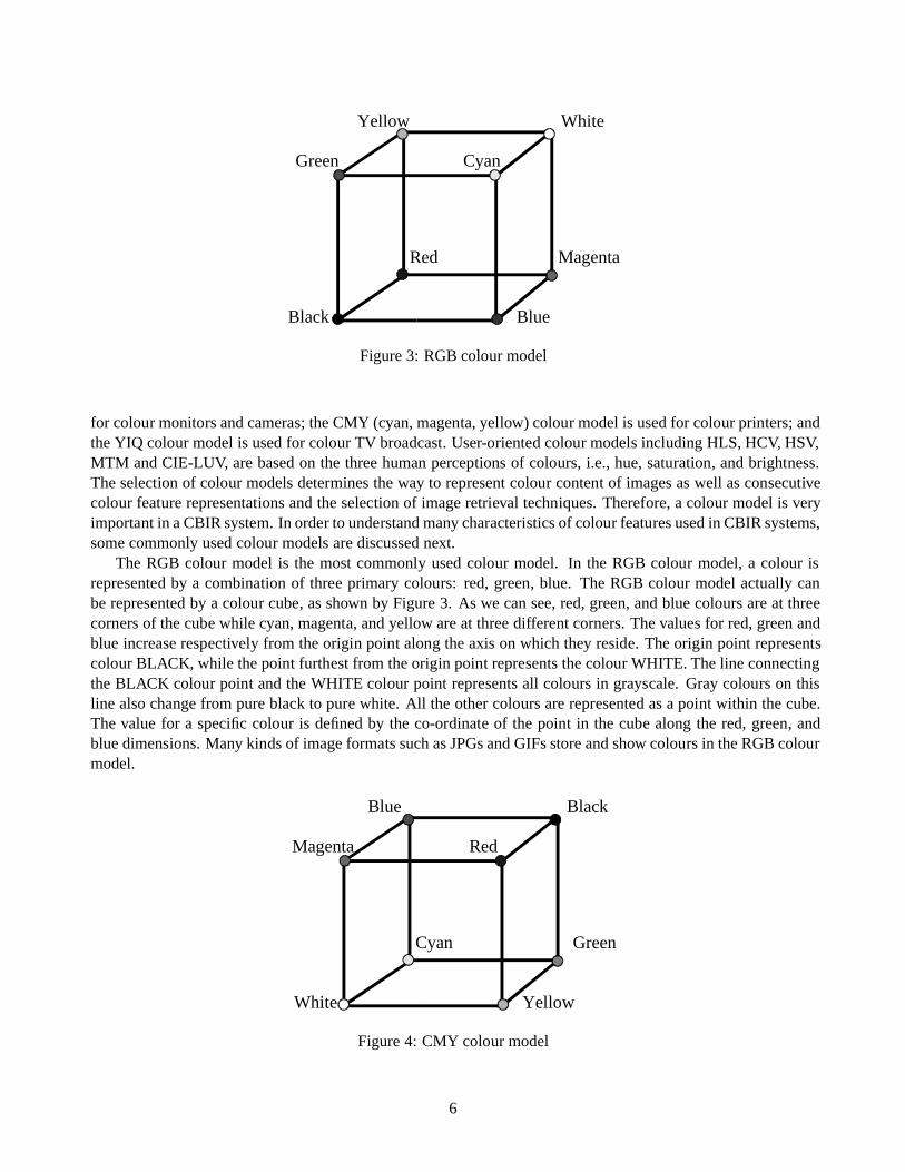
for colour monitors and cameras; the CMY (cyan, magenta, yellow) colour model is used for colour printers; andthe YIQ colour model is used for colour TV broadcast. User-oriented colour models including HLS, HCV, HSV,MTM and CIE-LUV, are based on the three human perceptions of colours, i.e., hue, saturation, and brightness.The selection of colour models determines the way to represent colour content of images as well as consecutivecolour feature representations and the selection of image retrieval techniques. Therefore, a colour model is veryimportant in a CBIR system. In order to understand many characteristics of colour features used in CBIR systems,some commonly used colour models are discussed next.
The RGB colour model is the most commonly used colour model. In the RGB colour model, a colour isrepresented by a combination of three primary colours: red, green, blue. The RGB colour model actually canbe represented by a colour cube, as shown by Figure 3. As we can see, red, green, and blue colours are at threecorners of the cube while cyan, magenta, and yellow are at three different corners. The values for red, green andblue increase respectively from the origin point along the axis on which they reside. The origin point representscolour BLACK, while the point furthest from the origin point represents the colour WHITE. The line connectingthe BLACK colour point and the WHITE colour point represents all colours in grayscale. Gray colours on thisline also change from pure black to pure white. All the other colours are represented as a point within the cube.The value for a specific colour is defined by the co-ordinate of the point in the cube along the red, green, andblue dimensions. Many kinds of image formats such as JPGs and GIFs store and show colours in the RGB colourmodel.
Blue Black
Magenta Red
Cyan Green
White Yellow
Figure 4: CMY colour model
6
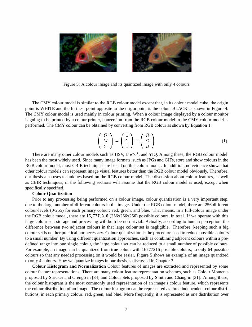
Figure 5: A colour image and its quantized image with only 4 colours
The CMY colour model is similar to the RGB colour model except that, in its colour model cube, the originpoint is WHITE and the furthest point opposite to the origin point is the colour BLACK as shown in Figure 4.The CMY colour model is used mainly in colour printing. When a colour image displayed by a colour monitoris going to be printed by a colour printer, conversion from the RGB colour model to the CMY colour model isperformed. The CMY colour can be obtained by converting from RGB colour as shown by Equation 1:����� � ��� ��� �� � �����
� ��(1)
There are many other colour models such as HSV, L��������� , and YIQ. Among these, the RGB colour modelhas been the most widely used. Since many image formats, such as JPGs and GIFs, store and show colours in theRGB colour model, most CBIR techniques are based on this colour model. In addition, no evidence shows thatother colour models can represent image visual features better than the RGB colour model obviously. Therefore,our thesis also uses techniques based on the RGB colour model. The discussion about colour features, as wellas CBIR techniques, in the following sections will assume that the RGB colour model is used, except whenspecifically specified.
Colour QuantizationPrior to any processing being performed on a colour image, colour quantization is a very important step,
due to the large number of different colours in the image. Under the RGB colour model, there are 256 differentcolour-levels (0-255) for each primary colour: red, green, and blue. That means, in a full-colour image underthe RGB colour model, there are
������������� !��(256x256x256) possible colours, in total. If we operate with this
large colour set, storage and processing will both be non-trivial. Actually, according to human perception, thedifference between two adjacent colours in that large colour set is negligible. Therefore, keeping such a bigcolour set is neither practical nor necessary. Colour quantization is the procedure used to reduce possible coloursto a small number. By using different quantization approaches, such as combining adjacent colours within a pre-defined range into one single colour, the large colour set can be reduced to a small number of possible colours.For example, an image can be quantized from true colour with 16777216 possible colours, to only 64 possiblecolours so that any needed processing on it would be easier. Figure 5 shows an example of an image quantizedto only 4 colours. How we quantize images in our thesis is discussed in Chapter 3.
Colour Histogram and Normalization Colour features of images are extracted and represented by somecolour feature representations. There are many colour feature representation schemes, such as Colour Momentsproposed by Stricker and Orengo in [34] and Colour Sets proposed by Smith and Chang in [31]. Among these,the colour histogram is the most commonly used representation of an image’s colour feature, which representsthe colour distribution of an image. The colour histogram can be represented as three independent colour distri-butions, in each primary colour: red, green, and blue. More frequently, it is represented as one distribution over
7

Figure 6: A colour image and its colour histogram
the three primaries, obtained by counting how many pixels in an image belong to each different colour. Figure 6shows an example image and its colour histogram.
Colour Number of pixels
(0, 0, 0) 234(0, 0, 1) 23(0, 0, 2) 478
. .
. .
. .(3, 3, 3) 3429
Table 1: Colour histogram for image A
The colour histogram for a given colour image � can be defined as��� �������� � ���� � �� ��� � � � ��� ��� � � �����where � is the number of quantization colours and
� �� is the number of pixels belonging to the � th colour.For example, the colour distribution of the colour image in Figure 6, quantized to 64 colours, is shown in Table 1.According to the numbers of pixels belonging to each of the 64 different colours, the colour histogram of thisimage is:
��� ��� ���� �� �������������� � � ������ �� �The use of actual pixel numbers to denote the colour distribution of an image is easy to understand and
manipulate. However, there is a problem when using this method to calculate the colour histograms for imagesof different sizes. Images of different sizes have different numbers of pixels. That means, for two images ofdifferent sizes, their colour histograms are not the same even when they have the same colour distributions. Forexample, suppose three images of different sizes are all quantized to 2 colours – black and white – as shown inFigure 7. The colour histograms for these three images are:
� � ��� ��� � !�� ��� � ���! ��� ���� ����"���� �� ���# ��� � � � � !��� � � � �As we can see, even though these three images have the same colour distributions, their colour histograms aredifferent from each other, due to their different sizes. In order to make all colour histograms the same for imageswith the same colour distributions, despite their sizes, histogram normalization is necessary. Instead of using theactual number of pixels of each colour, percentage of dividing the number by the total image pixels is used in
8
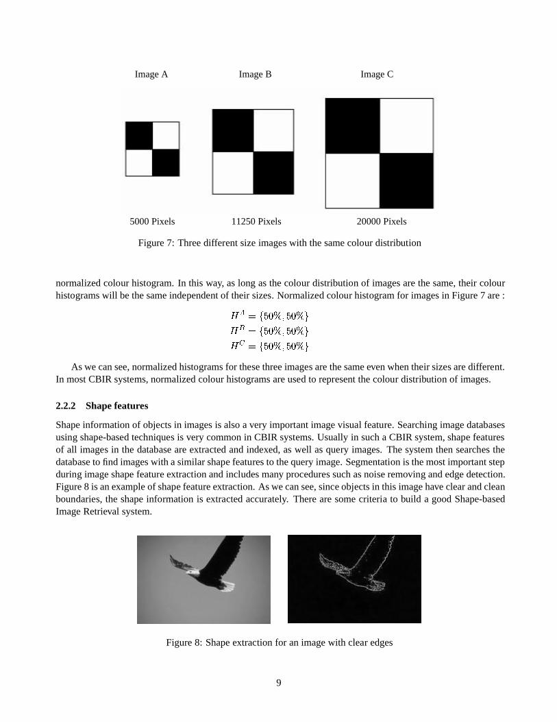
Image A Image B Image C
5000 Pixels 11250 Pixels 20000 Pixels
Figure 7: Three different size images with the same colour distribution
normalized colour histogram. In this way, as long as the colour distribution of images are the same, their colourhistograms will be the same independent of their sizes. Normalized colour histogram for images in Figure 7 are :
� � ��� �� �� �"�� �� �� ! ��� �� �� �"�� �� �� # ��� �� �� �"�� �� �As we can see, normalized histograms for these three images are the same even when their sizes are different.
In most CBIR systems, normalized colour histograms are used to represent the colour distribution of images.
2.2.2 Shape features
Shape information of objects in images is also a very important image visual feature. Searching image databasesusing shape-based techniques is very common in CBIR systems. Usually in such a CBIR system, shape featuresof all images in the database are extracted and indexed, as well as query images. The system then searches thedatabase to find images with a similar shape features to the query image. Segmentation is the most important stepduring image shape feature extraction and includes many procedures such as noise removing and edge detection.Figure 8 is an example of shape feature extraction. As we can see, since objects in this image have clear and cleanboundaries, the shape information is extracted accurately. There are some criteria to build a good Shape-basedImage Retrieval system.
Figure 8: Shape extraction for an image with clear edges
9
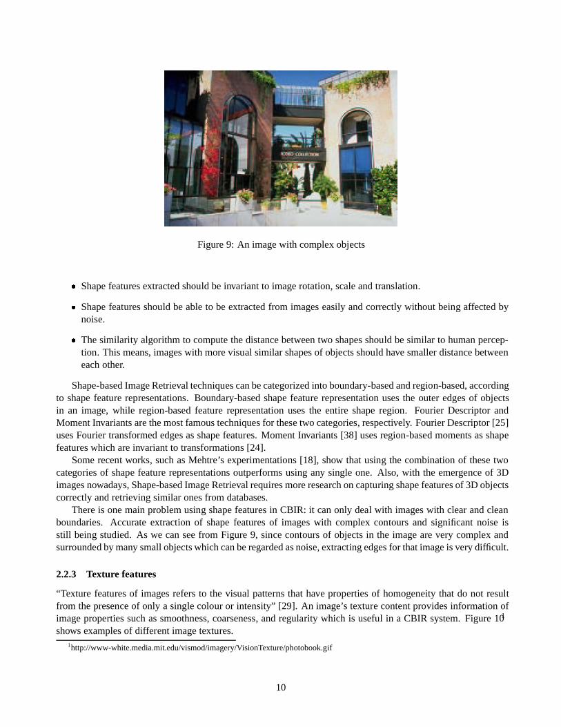
Figure 9: An image with complex objects
� Shape features extracted should be invariant to image rotation, scale and translation.
� Shape features should be able to be extracted from images easily and correctly without being affected bynoise.
� The similarity algorithm to compute the distance between two shapes should be similar to human percep-tion. This means, images with more visual similar shapes of objects should have smaller distance betweeneach other.
Shape-based Image Retrieval techniques can be categorized into boundary-based and region-based, accordingto shape feature representations. Boundary-based shape feature representation uses the outer edges of objectsin an image, while region-based feature representation uses the entire shape region. Fourier Descriptor andMoment Invariants are the most famous techniques for these two categories, respectively. Fourier Descriptor [25]uses Fourier transformed edges as shape features. Moment Invariants [38] uses region-based moments as shapefeatures which are invariant to transformations [24].
Some recent works, such as Mehtre’s experimentations [18], show that using the combination of these twocategories of shape feature representations outperforms using any single one. Also, with the emergence of 3Dimages nowadays, Shape-based Image Retrieval requires more research on capturing shape features of 3D objectscorrectly and retrieving similar ones from databases.
There is one main problem using shape features in CBIR: it can only deal with images with clear and cleanboundaries. Accurate extraction of shape features of images with complex contours and significant noise isstill being studied. As we can see from Figure 9, since contours of objects in the image are very complex andsurrounded by many small objects which can be regarded as noise, extracting edges for that image is very difficult.
2.2.3 Texture features
“Texture features of images refers to the visual patterns that have properties of homogeneity that do not resultfrom the presence of only a single colour or intensity” [29]. An image’s texture content provides information ofimage properties such as smoothness, coarseness, and regularity which is useful in a CBIR system. Figure 101
shows examples of different image textures.1http://www-white.media.mit.edu/vismod/imagery/VisionTexture/photobook.gif
10
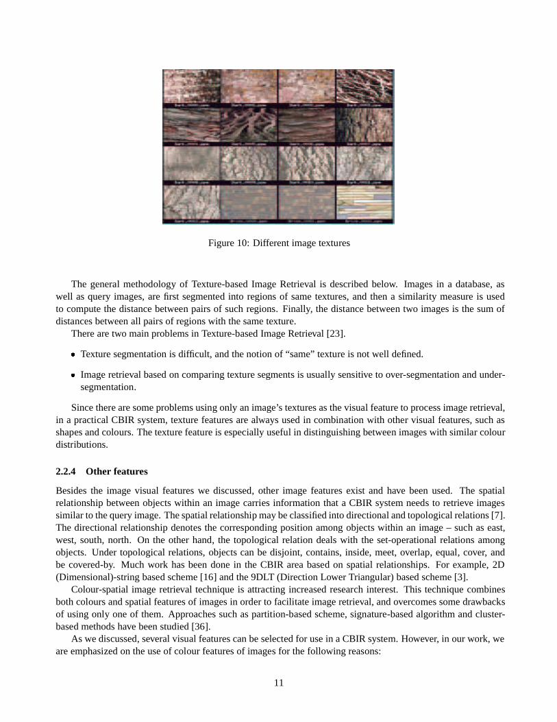
Figure 10: Different image textures
The general methodology of Texture-based Image Retrieval is described below. Images in a database, aswell as query images, are first segmented into regions of same textures, and then a similarity measure is usedto compute the distance between pairs of such regions. Finally, the distance between two images is the sum ofdistances between all pairs of regions with the same texture.
There are two main problems in Texture-based Image Retrieval [23].
� Texture segmentation is difficult, and the notion of “same” texture is not well defined.
� Image retrieval based on comparing texture segments is usually sensitive to over-segmentation and under-segmentation.
Since there are some problems using only an image’s textures as the visual feature to process image retrieval,in a practical CBIR system, texture features are always used in combination with other visual features, such asshapes and colours. The texture feature is especially useful in distinguishing between images with similar colourdistributions.
2.2.4 Other features
Besides the image visual features we discussed, other image features exist and have been used. The spatialrelationship between objects within an image carries information that a CBIR system needs to retrieve imagessimilar to the query image. The spatial relationship may be classified into directional and topological relations [7].The directional relationship denotes the corresponding position among objects within an image – such as east,west, south, north. On the other hand, the topological relation deals with the set-operational relations amongobjects. Under topological relations, objects can be disjoint, contains, inside, meet, overlap, equal, cover, andbe covered-by. Much work has been done in the CBIR area based on spatial relationships. For example, 2D(Dimensional)-string based scheme [16] and the 9DLT (Direction Lower Triangular) based scheme [3].
Colour-spatial image retrieval technique is attracting increased research interest. This technique combinesboth colours and spatial features of images in order to facilitate image retrieval, and overcomes some drawbacksof using only one of them. Approaches such as partition-based scheme, signature-based algorithm and cluster-based methods have been studied [36].
As we discussed, several visual features can be selected for use in a CBIR system. However, in our work, weare emphasized on the use of colour features of images for the following reasons:
11
� Colour is the most straightforward visual feature of images and is perceived by human beings immediately.
� Although shape and texture features can also be used in CBIR systems, they both have some limitationswhich are not involved in the use of colour features. For example, shape-based image retrieval can onlydeal with images with clear and clean boundaries while texture-based image retrieval has difficulty insegmentation for getting images’ textures.
� The colour feature of images can easily be extracted and manipulated in comparison with other features.
� Colour feature is still the most widely used visual feature in current CBIR systems [2].
Some colour-based image retrieval techniques are presented in the following sections.
2.3 Colour-based Image Retrieval Techniques
As mentioned, colour features are the most widely used in current CBIR systems. Many of these systems arebased on image colour histograms, in which distance between images is measured by calculating the distancebetween colour histograms. Different histogram distance metrics, as well as some Colour-based Image Retrievaltechniques, are discussed in this section.
2.3.1 Histogram Distance Metrics
There are a number of metrics for calculating the distance between two images’ histograms. As an example, toexplain different histogram distance metrics, we assume two images, A and B, are both quantized to 4 colours.Their normalized colour histograms are shown below:
� � ��� � �� �"�� �� ��� �� ��� �� ���! ��� � �� ��� �� �"�� �� �"�� �� �The simplest way to calculate the distance between the two colour histograms is L1 distance. It calculates
the absolute value of the difference between the same colours of two histograms and sums all of them as the totaldistance. As Equation 2 shows: ����� � ��� � ��
� ��� � �� � � !� � (2)
��� and� !� are the normalized values in the colour histogram of colour for image A and image B re-
spectively. � is the total number of colours. So, for our example, the distance between two images, A and B,is: ����� � ��� � �
� � � �����
� � � � �����
� � � ������
� � � � �� � � �
The distance between two histograms can also be calculated using L2 distance as Equation 3 shows:
����� � ��� � �������� ��� � �� � � !��� � (3)
��� ,� !� , , and � denote the same meaning as in Equation 2. For our example, the distance between the two
colour histograms using this metric is:
����� � ��� ��� � � � � � � � � � � � � � � � � � � � � � � � � � � � � � � � � � ���12
Using histogram intersection to calculate the distance between two colour histograms is another colour histogramdistance metric proposed by Swain and Ballard in [35]. Equation 4 shows the histogram intersection distancemetric between two colour histograms.
����� � ��� � � ��� ��� � � � � �� � � !� � (4)
Then, for our example, the distance using histogram intersection between two histograms is:����� � � � � � � � � � � �
� � � � � � �
There are also many other histogram distance metrics. Swain and Ballard also proposed an alternative tothe histogram intersection distance metric to improve retrieval effectiveness in large image databases, calledincremental intersection [35]. It only calculates the distance between histograms using the colours that have themost pixels in query and database images. Niblack et al. have used a distance measure called weighted Euclideandistance in the QBIC system to evaluate the similarity of colour histograms [21]. In [11], Flickner et al. haveproposed a simpler low-dimensional distance measure called average colour distance. Using this distance metricto calculate the distance between colour histograms can save significant time. However, L1-based and L2-basedhistogram distance metrics are still used the most widely in CBIR systems.
2.3.2 Global Colour Histogram (GCH) and Local Colour Histogram (LCH)
The GCH approach is the most popular Colour-based Image Retrieval technique and is often used as a benchmarkfor other techniques. In GCH, an image is represented by a single colour histogram to denote the whole contentof the image. Colour image indexing and retrieval are both based on this single colour histogram. The distancebetween two images is calculated using one of the colour histogram distance metrics discussed earlier based ontheir GCHs.
Now let us give an example to show how GCH works in Colour-based Image Retrieval. Suppose image Aand image B are the only two images in an image database. As shown in Figure 12, they are both quantized to 2colours: black and white. As we can see, the GCHs for these two images are:
� � � � �� � ����� � �� ! ��� �� �� �"�� �� �
The query image’s GCH as shown in Figure 11 is:
��������� ��� ��� � �� �� � �After we have the GCHs for all images in the image database, as well as the query image, different histogram
distance metrics can then be used. Suppose we use the L1-based histogram distance metric. The distance betweenthe query image and image A is: ����� � � � � �
� �� � � ������ �
� ��� � � ��� �
As well, the distance between the query image and image B is:����� � � � � � � � � � ���
� � � � � � � ��
� � � �Image B has a smaller distance to the query image than image A and, hence, Image B is supposed to be themost similar image in the database to the query image. Other histogram distance metrics such as L2-distance andhistogram intersection can also be used in GCH image retrieval.
13
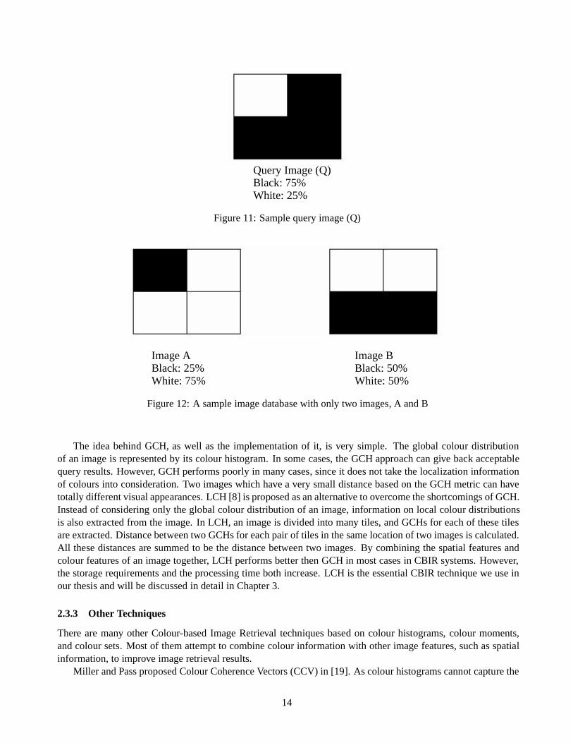
Query Image (Q) Black: 75%
White: 25%
Figure 11: Sample query image (Q)
Image A Image B Black: 25% Black: 50% White: 75% White: 50%
Figure 12: A sample image database with only two images, A and B
The idea behind GCH, as well as the implementation of it, is very simple. The global colour distributionof an image is represented by its colour histogram. In some cases, the GCH approach can give back acceptablequery results. However, GCH performs poorly in many cases, since it does not take the localization informationof colours into consideration. Two images which have a very small distance based on the GCH metric can havetotally different visual appearances. LCH [8] is proposed as an alternative to overcome the shortcomings of GCH.Instead of considering only the global colour distribution of an image, information on local colour distributionsis also extracted from the image. In LCH, an image is divided into many tiles, and GCHs for each of these tilesare extracted. Distance between two GCHs for each pair of tiles in the same location of two images is calculated.All these distances are summed to be the distance between two images. By combining the spatial features andcolour features of an image together, LCH performs better then GCH in most cases in CBIR systems. However,the storage requirements and the processing time both increase. LCH is the essential CBIR technique we use inour thesis and will be discussed in detail in Chapter 3.
2.3.3 Other Techniques
There are many other Colour-based Image Retrieval techniques based on colour histograms, colour moments,and colour sets. Most of them attempt to combine colour information with other image features, such as spatialinformation, to improve image retrieval results.
Miller and Pass proposed Colour Coherence Vectors (CCV) in [19]. As colour histograms cannot capture the
14
spatial information of an image, the CCV approach is a histogram-based scheme incorporating an image’s spatialinformation in order to calculate the distance between two images. A colour’s coherence is defined as the “degreeto which pixels of that colour are members of large similarly coloured regions”. These significant regions arereferred to as coherent regions. Based on whether the pixels belong to a part of some sizable contiguous regions,the CCV approach classifies all pixels of an image into coherent and incoherent pixels. A colour coherence vectorrepresents coherent and incoherent pixels for each different colour in an image. When calculating the distancebetween two images, coherent pixels in one image and incoherent pixels in another image will not match to eachother even if they belong to the same colour. Experiments show that using CCV allows better distinction betweenimages, which cannot be made using traditional colour histograms.
Based on the fact that humans intend to focus on large area of colours, rather than on small areas that arescattered around, a cluster-based image retrieval technique has been proposed by Tan, Ooi and Yee in [36].Colour-spatial information of an image is represented by a set of single-coloured clusters, and used to facilitateimage retrieval. Extracting clusters of an image consists of three phases. In the first phase, a set of colourswhich have the largest number of pixels in an image are selected. In the second phase, a cluster for each ofthese dominant colours is determined using a sequential 4-connected component algorithm. In phase three, theseclusters are ranked according to their sizes. Then the top � clusters are selected as the dominant clusters of theimage. Similarity between clusters of two images is calculated as the sum of overlapping pixel numbers for eachpair of clusters of the same colour.
The Colour Shape Histograms (CSH) was proposed by Stehling, Nascimento and Falcao in [32]. This ap-proach is based on the Local Colour Histogram and improves the colour histogram encoding of LCH. In LCH orGCH, the percentages of colours not presented in an image will be zero. In CSH, the colours not presented in animage will not be encoded into colour histograms at all. Experiments show that the number of actual differentcolours presented in an image is considerably fewer than the colours in the RGB colour model. In an image hav-ing N colours, there will be only N CSHs. This can reduce the storage of image colour histograms and increasethe efficiency of image retrieval.
In [34], the authors proposed a technique for image colour indexing based on colour moments. In theirapproach, different from GCH, an image’s colour content is represented by only their dominant features insteadof storing the complete colour distributions. They characterize a colour representation of image only by the firstthree colour moments: colour average, colour variance, and colour skewness. The distance between two imagesis calculated as a weighted sum of the absolute differences between corresponding moments. Thus, the similarityof images is determined by their colour moments. Through using this colour representation, low space overheadis achieved.
Colour histogram sets are proposed in [5] by Colombo, Rizzi and Genovesi to represent the local colour prop-erties of images. An image is segmented into a set of regions by dividing the image into small non-overlappingtiles, and then clustering them with a split and merge technique. Histogram intersection is then used to measurethe degree of colour distribution homogeneity between pairs of image regions. This approach is suitable forimages with regions having a colour distribution which significantly differs from the global colour distribution ofthe image. There are many other Colour-based Image Retrieval techniques, for an extensive survey refer to [2].
2.4 CBIR Systems
Since Content-based Image Retrieval has recently been an active research area, many different CBIR systemshave been developed. In this section, we select some of them and describe their characteristics.
Query By Image Content (QBIC) [21] is the first and most famous CBIR system and was developed by IBMAlmaden Research Center. It is available either in stand-alone form, or as part of other IBM products, such asthe DB2 digital library. Visual features used in QBIC include colours, shapes, and textures. The colour featuresused are 3-dimensional vector in RGB, YIQ, L ��� and Munsell colour model. The shape features consist of shapearea, circularity, eccentricity, major axis orientation, and a set of algebraic moment invariants [11]. Coarseness,
15
contrast, and directionality are texture features used in the system. In QBIC, different distance metrics such ashistogram-based algorithms are used to calculate the distance between two images. QBIC supports queries basedon example images, user-constructed sketches and drawings, selected colours, and texture patterns. A demo ofQBIC can be seen at http://wwwqbic.almaden.ibm.com.
The Photobook system [22] was developed by Pentland, Picard and Sclaroff from the Media Laboratory ofMIT, in 1995. It is a set of interactive tools for browsing and searching images in an image database. Thekey idea behind this suite of tools is semantic-preserving image compression, which reduces images to a smallset of perceptually significant coefficients. Photobook has been developed based on three different visual fea-tures: appearances, 2-dimensional shapes, and texture properties. All these representations can be combined toprovide users with a more sophisticated and efficient utility to browse and search images. Many distance met-rics such as Euclidean, mahalanobis, divergence, vector space angle, and Fourier peak are used in the system.Users can also define their own distance metrics in the latest version. A demo of Photobook can be found at:http://vismod.www.media.mit.edu/vismod/demos/photobook/index.html.
The VIRAGE Image Engine is another CBIR system, developed by Virage Technologies, Inc. It uses colours,shapes, and textures as visual features of images. These visual features can be used separately or combinedtogether to provide a more specific image searching. One of the advantages of using the VIRAGE system isthat users can adjust the weights associated with the atomic features according to their own emphasis [24]. AVIRAGE demo can be found at: http://www.virage.com/cgi-bin/query-e.
The image searching engine, NETRA, was developed by University of California, Santa Barbara [17]. Im-ages are segmented into regions with the same colour. For each of these regions, the colour, texture, shape andspatial features are extracted as visual features of images. These features can then be combined to search andretrieve similar regions from the database. In other words, this representation allows the user to compose in-teresting queries such as “retrieve all images that contain regions that have the colour of object A, texture ofobject B, shape of object C, and lie in the upper of the image” [17]. The online demo of Netra can be found at:http://vivaldi.ece.ucsb.edu/Netra/.
There are many other CBIR systems, such as Amore, developed by C&C Research Laboratories NEC [20],CANDID, developed by Los Alamos National Laboratory [15], ImageRover, developed by Boston Univ. [26],and Columbia University’s VisualSEEK&WebSEEK [28, 30].
3 Mosaicture Methodology
3.1 Image Mosaic and Related Work
An image has its own visual content, such as a bird flying in the sky or a little girl swimming in the sea. Ifseveral of these images are put together, what will the visual content of that large image be? Obviously, if manyimages are put together randomly, they will not suggest a meaningful content as a whole. Selecting images andputting them together, according to some methodology, in order to make the large image have its own meaningfulvisual content is an interesting topic which has been studied for a long time. These “big images” are called imagemosaics or image montages. Figure 13 shows such an image mosaic. The history of image mosaics as well assome existing image mosaic generating methodologies and products is discussed in the following sections.
3.1.1 Image Mosaics – History and Present
Building an image by combining many other images has a long history. Dating back to the 16th century, thepainter Giuseppe Arcimboldo manually put pictures of vegetables, fruit and flowers together to build a wholeimage. American painter, Chuck Close, generate many portrait using greyscale blocks. Figure 14 shows oneof his self-portraits. In November 1973, an article, “The Recognition of Faces”, written by Leon Harmon, andwhich used a portrait of Lincoln as an example of recognizing human faces, was published in Scientific American.
16

Different from common images, Lincoln’s face in this portrait is suggested by combining together many grayscaleblocks. In 1976, instead of using just grayscale blocks, Salvador Dali used small colour images to build an imagemosaic of the same portrait. In Dali’s work, he put his wife’s picture in the center of Lincoln’s face with someother small images of Lincoln himself scattered around. This mosaic image is likely one of the most famous artworks in this area and is shown in Figure 1 in Chapter 1.
With the advent of advanced computer technologies, both artists and computer scientists are trying to buildimage mosaics with the help of computers.
A famous image mosaic generating system using computers is Robert Silver’s “Photomosaic” [27]. Thissystem generates an image mosaic by putting many images together according to some algorithms. Different op-tions are available for users to control the generating process. Robert Silvers patented his technique of building
Figure 13: An image mosaic of landscape by Mosaic Magic [1]
Figure 14: Chunk Close’s self-portrait
17
image mosaics in 1996. His company, Runaway Technology, now generates image mosaics for many organiza-tions, companies, and academic institutions. Many of his image mosaic products can be seen on the Internet athttp://www.photomosaic.com.
Obviously, image mosaics have their value both in arts and entertainment. In addition, image mosaics canalso be used in the area of copyright protection. For instance, it is not safe to let just anybody have access tosome original priceless masterpiece of art. Reproductions of these original art works can be produced in theformat of image mosaics which can then be shown to people. People can still see the content of the art work, butthey cannot produce fake works based on these previews, due to the insufficient information contained. Otherapplications of image mosaics, such as compression and complexity theory, are discussed in detail in [37].
3.1.2 General scheme of image mosaic generating systems
Typically, an image mosaic is generated as a reproduction of its original image. In other words, when an imagecalled the original image is given, many images are put together to build an image mosaic which has a similarvisual content to the original image. The typical scheme of generating image mosaics is described below.
In an image mosaic generating system, thousands of images, which will be used as building blocks to generatean image mosaic, are contained in an image database. All these database images are pre-processed by the system.During this step, visual features such as colours, shapes, and textures are extracted from database images andstored as metadata of real images. When an original image is given, it is divided into many blocks called tiles.Then for each tile, the same visual features are extracted and used to match the metadata of database images.According to some criteria, the image in the database with the most similar visual content is selected as the bestmatching image for that tile. Finally, all these best matching images for each tile are combined to build up animage mosaic reproduction of the original image. For the purpose of making the content of an image mosaicgenerating system understandable through this thesis, some terms we just used to describe the image mosaicgenerating process are explained below:
� Original image - The image based on which an image mosaic reproduction is generated.
� Target image - The final image mosaic reproduction of the original image.
� DB image - The source image in an image database which is used to build an image mosaic.
� Tile - When an original image is divided into many small blocks, each of these small blocks is called a tile.
� Best matching image - The image within an image database that is considered by the system having themost similar visual content to a tile.
3.1.3 Existing Methodologies and Products
Even though building image mosaics is an interesting topic, it still has not been studied widely. However, wedescribe some existing methodologies as well as introducing some commercial products in this section as thebackground of our research.
As mentioned previously, Robert Silvers’ patent system “Photomosaic” is probably the most famous imagemosaic generating system. In Silvers’ Photomosaic system, DB images can be both regular images and snapshotscaptured from other devices, such as a VHS video tape player. In addition, these images are cropped to be squarein the same dimension. All these DB images are classified into many categories according to their semanticcontent such as animals, humans, and nature. Users of the system can select using DB images in a specificcategory to generate an image mosaic. Also, these DB images are stored in different resolutions. Images in lowresolution are used to generate an image mosaic, while images in high resolution are used to print out a poster ofthe bigger image. When an original image is loaded into the system, it is divided into many tiles. For each tile,
18
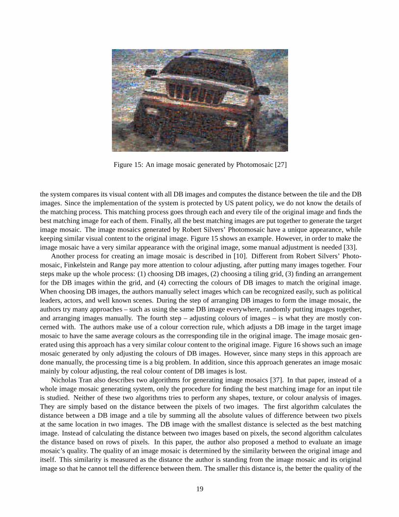
Figure 15: An image mosaic generated by Photomosaic [27]
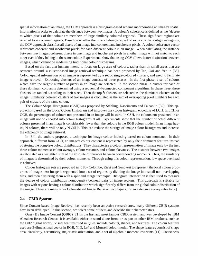
the system compares its visual content with all DB images and computes the distance between the tile and the DBimages. Since the implementation of the system is protected by US patent policy, we do not know the details ofthe matching process. This matching process goes through each and every tile of the original image and finds thebest matching image for each of them. Finally, all the best matching images are put together to generate the targetimage mosaic. The image mosaics generated by Robert Silvers’ Photomosaic have a unique appearance, whilekeeping similar visual content to the original image. Figure 15 shows an example. However, in order to make theimage mosaic have a very similar appearance with the original image, some manual adjustment is needed [33].
Another process for creating an image mosaic is described in [10]. Different from Robert Silvers’ Photo-mosaic, Finkelstein and Range pay more attention to colour adjusting, after putting many images together. Foursteps make up the whole process: (1) choosing DB images, (2) choosing a tiling grid, (3) finding an arrangementfor the DB images within the grid, and (4) correcting the colours of DB images to match the original image.When choosing DB images, the authors manually select images which can be recognized easily, such as politicalleaders, actors, and well known scenes. During the step of arranging DB images to form the image mosaic, theauthors try many approaches – such as using the same DB image everywhere, randomly putting images together,and arranging images manually. The fourth step – adjusting colours of images – is what they are mostly con-cerned with. The authors make use of a colour correction rule, which adjusts a DB image in the target imagemosaic to have the same average colours as the corresponding tile in the original image. The image mosaic gen-erated using this approach has a very similar colour content to the original image. Figure 16 shows such an imagemosaic generated by only adjusting the colours of DB images. However, since many steps in this approach aredone manually, the processing time is a big problem. In addition, since this approach generates an image mosaicmainly by colour adjusting, the real colour content of DB images is lost.
Nicholas Tran also describes two algorithms for generating image mosaics [37]. In that paper, instead of awhole image mosaic generating system, only the procedure for finding the best matching image for an input tileis studied. Neither of these two algorithms tries to perform any shapes, texture, or colour analysis of images.They are simply based on the distance between the pixels of two images. The first algorithm calculates thedistance between a DB image and a tile by summing all the absolute values of difference between two pixelsat the same location in two images. The DB image with the smallest distance is selected as the best matchingimage. Instead of calculating the distance between two images based on pixels, the second algorithm calculatesthe distance based on rows of pixels. In this paper, the author also proposed a method to evaluate an imagemosaic’s quality. The quality of an image mosaic is determined by the similarity between the original image anditself. This similarity is measured as the distance the author is standing from the image mosaic and its originalimage so that he cannot tell the difference between them. The smaller this distance is, the better the quality of the
19

Figure 16: Generating an image mosaic by adjusting colours [10]
image mosaic. The two algorithms proposed in Tran’s paper are easy to understand and implement. However,both of them just use the very simple pixel-by-pixel-based algorithm to calculate the distance between an imageand a tile, which do not take the global content into consideration. Also, their method of evaluating the qualityof an image mosaic is purely based on human perception. Even though human eye can be considered as the bestway to evaluate an image mosaic’s quality, it is not practical to evaluate hundreds of image mosaics, one by one,using this method.
In addition to what we have discussed above, there are other commercial products for generating imagemosaics. PhotoShop2 from Adobe cannot build image mosaics automatically, but it is still possible to manuallymanipulate images and combine them to form a large image. ArcSoft’s PhotoMontage3 is another commercialproduct which can build image mosaics automatically. It provides users many options to control the image mosaicgenerating process, such as the number of times a DB image can occur in an image mosaic. Users can also addtheir own images into the image database included in this software. Figure 17 shows an image mosaic generatedby Photomontage. Mosaic Magic [1] is a free software for building image mosaics, which also permits users toadd their own images to the existing database. In addition, it provides a colour adjusting function with whichusers can adjust the colour of an image mosaic to get a better result.
3.2 Mosaicture – Our Image Mosaic Generating Methodology
3.2.1 Architecture of the system
Mosaicture, the image mosaic generating methodology that we propose, is implemented as an image mosaicgenerating system in our thesis. The whole system consists of two main stages, as shown in Figure 18:
� Image Database Pre-processing Stage.
� Image Mosaic Generating Stage.2http://www.adobe.com/products/photoshop/main.html3http://www.arcsoft.com/products/software/en/photomontage2000.html
20
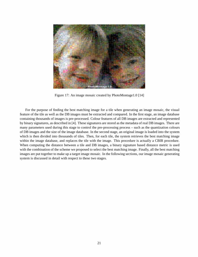
Figure 17: An image mosaic created by PhotoMontage1.0 [14]
For the purpose of finding the best matching image for a tile when generating an image mosaic, the visualfeature of the tile as well as the DB images must be extracted and compared. In the first stage, an image databasecontaining thousands of images is pre-processed. Colour features of all DB images are extracted and representedby binary signatures, as described in [4]. These signatures are stored as the metadata of real DB images. There aremany parameters used during this stage to control the pre-processing process – such as the quantization coloursof DB images and the size of the image database. In the second stage, an original image is loaded into the systemwhich is then divided into thousands of tiles. Then, for each tile, the system retrieves the best matching imagewithin the image database, and replaces the tile with the image. This procedure is actually a CBIR procedure.When computing the distance between a tile and DB images, a binary signature based distance metric is usedwith the combination of the scheme we proposed to select the best matching image. Finally, all the best matchingimages are put together to make up a target image mosaic. In the following sections, our image mosaic generatingsystem is discussed in detail with respect to these two stages.
21

Figure 18: The system architecture of Mosaicture
22
3.2.2 The image database pre-processing stage
In our system, the image database pre-processing stage includes many procedures such as extracting visual fea-tures from DB images and representing visual features with abstract representations. All these procedures, aswell as some parameters used, are discussed in detail in the following sections.
Selecting DB Images
An image database contains all the DB images for generating image mosaics. First, we select our DB images.There are some factors we need to take into consideration, such as the format of images and the number of imagesin the database. There are many different image formats available such as JPGs, GIFs, and BMPs. Among theseimage formats, JPG images are the most widely used in digital archives, as well as on the Internet. In comparisonwith other image formats, JPG images are smaller in size, while maintaining good quality at the same time. Inaddition, JPG images use the RGB colour model, which is simple and easy to manipulate. Thus, we select imagesin JPG format to make up our image database. We also need to decide how many DB images we should have inthe database; this is actually a parameter in our system. This parameter affects the processing time for generatingan image mosaic, as well as the target image mosaic’s quality. Typically, the more DB images we have, the betterthe target image mosaic will be, as well as the more processing time is spent to generate such an image mosaic.Analysis of the experimental results of this parameter will be discussed in detail in Chapter 4.
Image Quantization
Since colour features are the most straightforward visual features of images, we use CBIR techniques basedon colour features when searching the best matching image for the tiles of an original image. Before we canextract colour features from DB images, colour quantization is a necessary step. As mentioned in Chapter2, colour quantization is used to reduce the number of colours of a full-colour image. There are two maincolour quantization approaches: Uniform Colour Quantization and Non-uniform Colour Quantization. In thefirst approach, all images are quantized to the same set of colours. These colours are produced by combiningmany different colours within a pre-defined range into a single colour. In the non-uniform quantization approach,more colours might be used in the colour levels that are perception-sensitive. Under this approach, differentimages might be quantized to different sets of colours due to their different colour contents.
In our work, we need to compare an input tile of an original image with all DB images in order to find itsbest matching image. We therefore select using the uniform quantization approach to quantize all images to thesame set of colours. As mentioned in Chapter 2, the RGB colour model can be viewed as a cube; any single pointwithin this cube represents a colour. When we perform the uniform colour quantization, we divide this cube intomany sub-cubes by separating each axis, Red, Green, and Blue into the same number of sub-divisions. Each ofthese sub-cubes represents a quantized colour. Figure 19 shows an example of producing 64 quantization colours.In this example, each axis is divided into 4 sub-divisions, thus the cube is divided into 64 (
� ) sub-cubes. Each
of these 64 sub-cubes represents a single colour after quantization.In our work, a colour (R, G, B) in a true-colour image is converted to the colour (r, g, b) in a quantized colour
space according to Equation 5, ������
�� � ������ ��� ������ ��� ����� � ��� ���� �� (5)
where � is the number of sub-divisions into which each of the three primary colours is divided. For example, atrue colour (23, 242, 162) is converted to the colour (
���� � � ���� , �� �� � � ���� , ��� � � � ���� ) in a�
quantizationcolour space. In other words, the original colour is converted to (0, 3, 2).
There is no best number of quantization colours. Typically, the fewer colours used, the faster and more easilyan image can be manipulated, but in the mean time, the more colour information of an image is lost. Actually, the
23
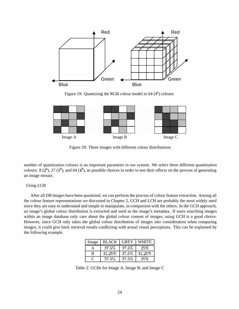
Red Red
Green GreenBlue Blue
Figure 19: Quantizing the RGB colour model to 64 (�
) colours
Image A Image B Image C
Figure 20: Three images with different colour distributions
number of quantization colours is an important parameter in our system. We select three different quantizationcolours: 8 (
), 27 (
� ), and 64 (
� ), as possible choices in order to test their effects on the process of generating
an image mosaic.
Using LCH
After all DB images have been quantized, we can perform the process of colour feature extraction. Among allthe colour feature representations we discussed in Chapter 2, GCH and LCH are probably the most widely usedsince they are easy to understand and simple to manipulate, in comparison with the others. In the GCH approach,an image’s global colour distribution is extracted and used as the image’s metadata. If users searching imageswithin an image database only care about the global colour content of images, using GCH is a good choice.However, since GCH only takes the global colour distribution of images into consideration when comparingimages, it could give back retrieval results conflicting with actual visual perceptions. This can be explained bythe following example.
Image BLACK GREY WHITE
A� � � � � � � � � � �� �
B�!�� �� � � � � � � �!�� �� �
C� � � � � � � � � � �� �
Table 2: GCHs for Image A, Image B, and Image C
24
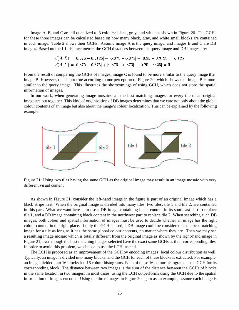
Image A, B, and C are all quantized to 3 colours: black, gray, and white as shown in Figure 20. The GCHsfor these three images can be calculated based on how many black, gray, and white small blocks are containedin each image. Table 2 shows their GCHs. Assume image A is the query image, and images B and C are DBimages. Based on the L1 distance metric, the GCH distances between the query image and DB images are:
����� � � � � � � � ��� � � �!� ��
� � � � � ��� � � � ���
����� � �� � � �!� ��
� � � � ������� ��� � � �
� � ��� � � � ���� � �
� � ��� � � � ���� ���
� �� � � ��� �
From the result of comparing the GCHs of images, image C is found to be more similar to the query image thanimage B. However, this is not true according to our perception of Figure 20, which shows that image B is moresimilar to the query image. This illustrates the shortcomings of using GCH, which does not store the spatialinformation of images.
In our work, when generating image mosaics, all the best matching images for every tile of an originalimage are put together. This kind of organization of DB images determines that we care not only about the globalcolour contents of an image but also about the image’s colour localization. This can be explained by the followingexample.
Figure 21: Using two tiles having the same GCH as the original image may result in an image mosaic with verydifferent visual content
As shown in Figure 21, consider the left-hand image in the figure is part of an original image which has ablack stripe in it. When the original image is divided into many tiles, two tiles, tile 1 and tile 2, are containedin this part. What we want here is to use a DB image containing black content in its southeast part to replacetile 1, and a DB image containing black content in the northwest part to replace tile 2. When searching such DBimages, both colour and spatial information of images must be used to decide whether an image has the rightcolour content in the right place. If only the GCH is used, a DB image could be considered as the best matchingimage for a tile as long as it has the same global colour contents, no matter where they are. Then we may seea resulting image mosaic which is totally different from the original image as shown by the right-hand image inFigure 21, even though the best matching images selected have the exact same GCHs as their corresponding tiles.In order to avoid this problem, we choose to use the LCH instead.
The LCH is proposed as an improvement of the GCH by encoding images’ local colour distribution as well.Typically, an image is divided into many blocks, and the GCH for each of these blocks is extracted. For example,an image divided into 16 blocks has 16 colour histograms. Each of these 16 colour histograms is the GCH for itscorresponding block. The distance between two images is the sum of the distance between the GCHs of blocksin the same location in two images. In most cases, using the LCH outperforms using the GCH due to the spatialinformation of images encoded. Using the three images in Figure 20 again as an example, assume each image is
25
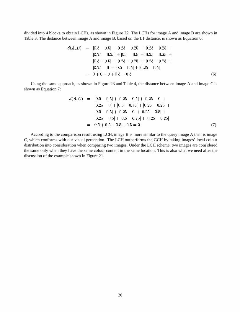
divided into 4 blocks to obtain LCHs, as shown in Figure 22. The LCHs for image A and image B are shown inTable 3. The distance between image A and image B, based on the L1 distance, is shown as Equation 6:
����� � � � � � � � � � �
� � � � �� � � ��
��� � � �� � � ��
���� � �� � � ��
��� � � � � � �
��� � � �� � � ��
���� � � � � �
� � � � �� � � ��
��� � � �� � � ��
���� � �� �
� � � � � � � �
� � � � �� � � �
�� � � � � � � � �
(6)
Using the same approach, as shown in Figure 23 and Table 4, the distance between image A and image C isshown as Equation 7:
����� ��� � � � � � � � �
��� � � �� � � �
� � � � �� �
� �� � �� �
��� � � � � � ���
� � � � �� � � ��
���� � � � � �
��� � � �� �
��� � � �� � � �
� �� � �� � � �
� � � � � � � ��
� � � � �� � � ��
�� � �� � �
� � �
� � � �
(7)
According to the comparison result using LCH, image B is more similar to the query image A than is imageC, which conforms with our visual perception. The LCH outperforms the GCH by taking images’ local colourdistribution into consideration when comparing two images. Under the LCH scheme, two images are consideredthe same only when they have the same colour content in the same location. This is also what we need after thediscussion of the example shown in Figure 21.
26
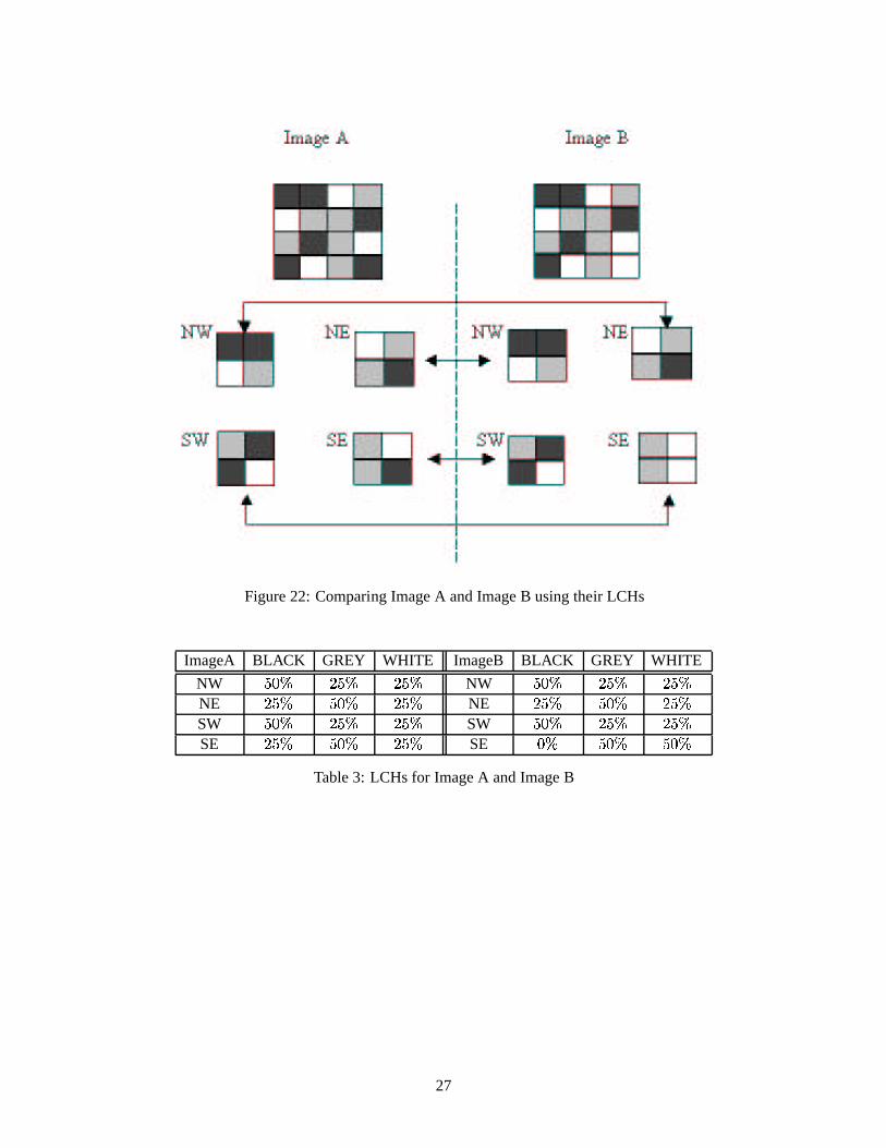
Figure 22: Comparing Image A and Image B using their LCHs
ImageA BLACK GREY WHITE ImageB BLACK GREY WHITE
NW�� �� �� � �� �
NW�� �� �� � �� �
NE �� � �� �� �� �
NE �� � �� �� �� �
SW�� �� �� � �� �
SW�� �� �� � �� �
SE �� � �� �� �� �
SE �� �� �� �� ��
Table 3: LCHs for Image A and Image B
27
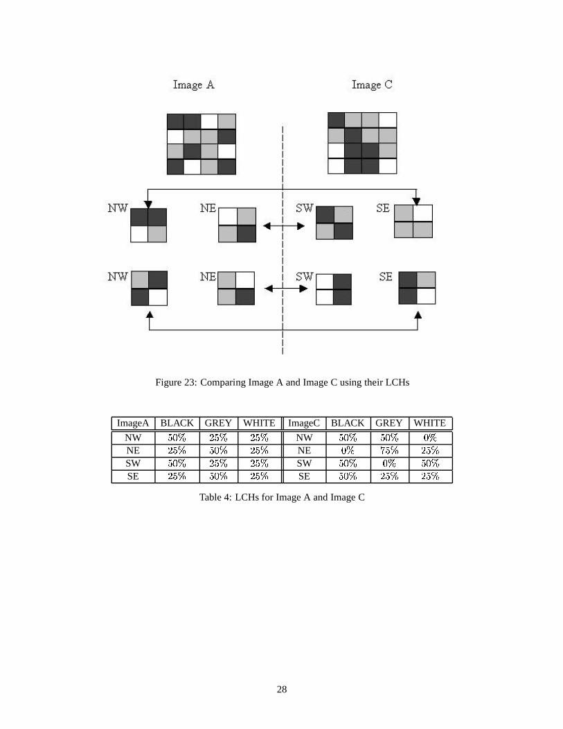
Figure 23: Comparing Image A and Image C using their LCHs
ImageA BLACK GREY WHITE ImageC BLACK GREY WHITE
NW�� �� �� � �� �
NW�� �� �� �� ��
NE �� � �� �� �� �
NE �� ��� � �� �
SW�� �� �� � �� �
SW�� �� �� �� ��
SE �� � �� �� �� �
SE�� �� �� � �� �
Table 4: LCHs for Image A and Image C
28
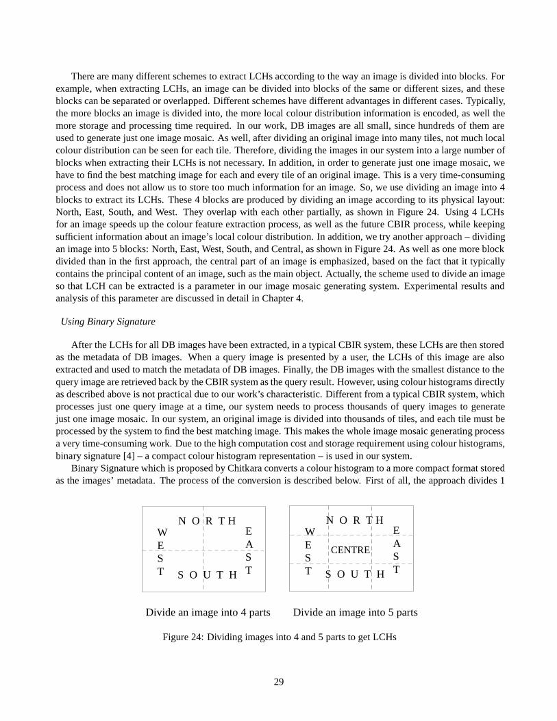
There are many different schemes to extract LCHs according to the way an image is divided into blocks. Forexample, when extracting LCHs, an image can be divided into blocks of the same or different sizes, and theseblocks can be separated or overlapped. Different schemes have different advantages in different cases. Typically,the more blocks an image is divided into, the more local colour distribution information is encoded, as well themore storage and processing time required. In our work, DB images are all small, since hundreds of them areused to generate just one image mosaic. As well, after dividing an original image into many tiles, not much localcolour distribution can be seen for each tile. Therefore, dividing the images in our system into a large number ofblocks when extracting their LCHs is not necessary. In addition, in order to generate just one image mosaic, wehave to find the best matching image for each and every tile of an original image. This is a very time-consumingprocess and does not allow us to store too much information for an image. So, we use dividing an image into 4blocks to extract its LCHs. These 4 blocks are produced by dividing an image according to its physical layout:North, East, South, and West. They overlap with each other partially, as shown in Figure 24. Using 4 LCHsfor an image speeds up the colour feature extraction process, as well as the future CBIR process, while keepingsufficient information about an image’s local colour distribution. In addition, we try another approach – dividingan image into 5 blocks: North, East, West, South, and Central, as shown in Figure 24. As well as one more blockdivided than in the first approach, the central part of an image is emphasized, based on the fact that it typicallycontains the principal content of an image, such as the main object. Actually, the scheme used to divide an imageso that LCH can be extracted is a parameter in our image mosaic generating system. Experimental results andanalysis of this parameter are discussed in detail in Chapter 4.
Using Binary Signature
After the LCHs for all DB images have been extracted, in a typical CBIR system, these LCHs are then storedas the metadata of DB images. When a query image is presented by a user, the LCHs of this image are alsoextracted and used to match the metadata of DB images. Finally, the DB images with the smallest distance to thequery image are retrieved back by the CBIR system as the query result. However, using colour histograms directlyas described above is not practical due to our work’s characteristic. Different from a typical CBIR system, whichprocesses just one query image at a time, our system needs to process thousands of query images to generatejust one image mosaic. In our system, an original image is divided into thousands of tiles, and each tile must beprocessed by the system to find the best matching image. This makes the whole image mosaic generating processa very time-consuming work. Due to the high computation cost and storage requirement using colour histograms,binary signature [4] – a compact colour histogram representation – is used in our system.
Binary Signature which is proposed by Chitkara converts a colour histogram to a more compact format storedas the images’ metadata. The process of the conversion is described below. First of all, the approach divides 1
Divide an image into 4 parts Divide an image into 5 parts
N O R T H
S O U T H
WEST
EAST
N O R T H
S O U T H
WEST
EAST
CENTRE
Figure 24: Dividing images into 4 and 5 parts to get LCHs
29
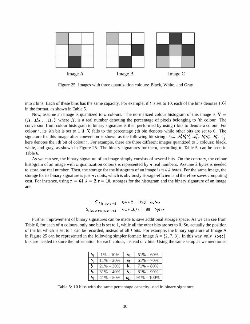
Image A Image B Image C
Figure 25: Images with three quantization colours: Black, White, and Gray
into � bins. Each of these bins has the same capacity. For example, if � is set to 10, each of the bins denotes� ��
in the format, as shown in Table 5.Now, assume an image is quantized to � colours. The normalized colour histogram of this image is
� �� � � � � � ��� � � � � � � , where� � is a real number denoting the percentage of pixels belonging to � th colour. The
conversion from colour histogram to binary signature is then performed by using � bits to denote a colour. Forcolour � , its th bit is set to 1 if
� � falls to the percentage th bin denotes while other bits are set to 0. Thesignature for this image after conversion is shown as the following bit-string: �
�� � �� � � � � �� � � � � �� � � � � �� � � � � � � � � � � � � � �� . ���
here denotes the th bit of colour � . For example, there are three different images quantized to 3 colours: black,white, and gray, as shown in Figure 25. The binary signatures for them, according to Table 5, can be seen inTable 6.
As we can see, the binary signature of an image simply consists of several bits. On the contrary, the colourhistogram of an image with � quantization colours is represented by � real numbers. Assume � bytes is neededto store one real number. Then, the storage for the histogram of an image is � � � bytes. For the same image, thestorage for its binary signature is just � � � bits, which is obviously storage-efficient and therefore saves computingcost. For instance, using � � ��� � � � �� � � �
, storages for the histogram and the binary signature of an imageare:
����� ��� ������ ���� � ��� � � � �����������
� ��� � � ���� � � � ��������� � ��� � � � � � �� ���������
Further improvement of binary signatures can be made to save additional storage space. As we can see fromTable 6, for each of � colours, only one bit is set to 1, while all the other bits are set to 0. So, actually the positionof the bit which is set to 1 can be recorded, instead of all � bits. For example, the binary signature of Image Ain Figure 25 can be represented in the following simpler format: Image A =
�2, 7, 3 � . In this way, only "!$# � � �%
bits are needed to store the information for each colour, instead of � bits. Using the same setup as we mentioned
� � 1% – 10% ��& 51% – 60%� � 11% – 20% ��' 61% – 70%� 21% – 30% ��( 71% – 80%��) 31% – 40% ��* 81% – 90%�,+ 41% – 50% � �.- 91% – 100%
Table 5: 10 bins with the same percentage capacity used in binary signature
30

Binary SignatureColour Histogram � � � � � ��) �,+ �,& � ' �,( �,* � �.-
Image ABlack 11% 0 1 0 0 0 0 0 0 0 0White 67% 0 0 0 0 0 0 1 0 0 0Grey 22% 0 0 1 0 0 0 0 0 0 0Binary Signature 010000000000000010000010000000
Image BBlack 22% 0 0 1 0 0 0 0 0 0 0White 67% 0 0 0 0 0 0 1 0 0 0Grey 11% 0 1 0 0 0 0 0 0 0 0Binary Signature 001000000000000010000100000000
Image CBlack 33% 0 0 0 1 0 0 0 0 0 0White 33% 0 0 0 1 0 0 0 0 0 0Grey 33% 0 0 0 1 0 0 0 0 0 0Binary Signature 000100000000010000000001000000
Table 6: Binary Signatures for Image A, B, and C using CBA
above, � � ��� �� � �� � � �
, the storage for the improved binary signature of an image, which saves 75%storage space in comparison to its colour histogram is shown as:
� � � ��������������� � � � ������ � � � ��������� � ��� � "!$# � � � % � �� ������� �
The binary signatures that we discussed above are converted from colour histograms by dividing 1 into � binshaving the same capacity. This scheme is called Constant-Bin Allocation (CBA). There is also another scheme –Variable-Bin Allocation (VBA) – proposed in [4]. As an alternative approach to CBA, VBA is based on varyingthe capacity of each bin. The design of VBA is based on the fact that distances due to less dominant colours areimportant for efficient image retrieval. The VBA signature of an image puts more emphasis on less dominantcolours than on larger dominant colours. As proved by experimental results in [4], use of the VBA signatureoutperforms using CBA.
Table 7 shows the best variable bin allocation proved by [4] when � is set to 10. This bin allocation schemeis what we used in our work. Using the VBA approach, as shown in Table 7, the binary signatures of Images A,B, and C in Figure 25 are shown in Table 8.
In our work, normalized LCHs are extracted from all DB images and then transferred to binary signatures,using the VBA approach, as shown in Table 7. All the binary signatures for the same block of DB images are
� � 1% – 3% ��& 21% – 30%� � 4% – 6% � ' 31% – 40%� 7% – 10% ��( 41% – 50%� ) 11% – 15% � * 51% – 60%�,+ 16% – 20% � �.- 61% – 100%
Table 7: Variable bin allocation used in binary signature
31

Binary SignatureColour Histogram � � � � � ��) �,+ �,& � ' �,( �,* � �.-
Image ABlack 11% 0 0 0 1 0 0 0 0 0 0White 67% 0 0 0 0 0 0 0 0 0 1Grey 22% 0 0 0 0 0 1 0 0 0 0Binary Signature 000100000000000000010000010000
Image BBlack 22% 0 0 0 0 0 1 0 0 0 0White 67% 0 0 0 0 0 0 0 0 0 1Grey 11% 0 0 0 1 0 0 0 0 0 0Binary Signature 000001000000000000010001000000
Image CBlack 33% 0 0 0 0 0 0 1 0 0 0White 33% 0 0 0 0 0 0 1 0 0 0Grey 33% 0 0 0 0 0 0 1 0 0 0Binary Signature 000000100000000010000000001000
Table 8: Binary Signatures for Image A, B, and C using VBA
stored in the same file. For example, when extracting an image’s LCH by dividing it into 4 blocks, there are 4 filescreated. Each file contains all the signatures for all DB images of the same block. In image mosaic generatingstage which will be discussed later, searching the best matching image for a tile of an original image is based onthese binary signatures.
3.2.3 The image mosaic generating stage
As shown in Figure 18, an original image is loaded into our system and then divided into many tiles of the samesize. After the original image has been tiled, each tile is regarded as an image and is processed in the same wayas all DB images, as we described in the last section. First of all, a tile is quantized to the same set of coloursas all DB images, then the tile is divided into blocks to extract its LCHs. After that, all LCHs are translated tobinary signatures using the same bin allocation scheme as all DB images. Until now, the tile has the same numberof binary signatures in the same format as all DB images. The approach we proposed to find the best matchingimage for a tile can then be used, based on these signatures. The basic idea of our approach is to select a set ofDB images as candidate images according to the distance between their binary signatures and the input tile; then,the best matching image for the tile is selected among these candidate images. The same process goes througheach and every tile of the original image. Finally, the target image mosaic is generated by substituting each tileby its best matching image. Our proposed approach to find the best matching image for a tile, which plays themost important role in the whole image mosaic generating stage, is described in detail in the next subsection.
Finding the best matching image for a tileIn order to find the best matching image for a tile, the distance between each DB image and the tile is
calculated. The DB image with the smallest distance is considered as the best matching image. As we mentionedbefore, in the typical LCH-based image retrieval, the distance between a tile and a DB image is the sum of all
32
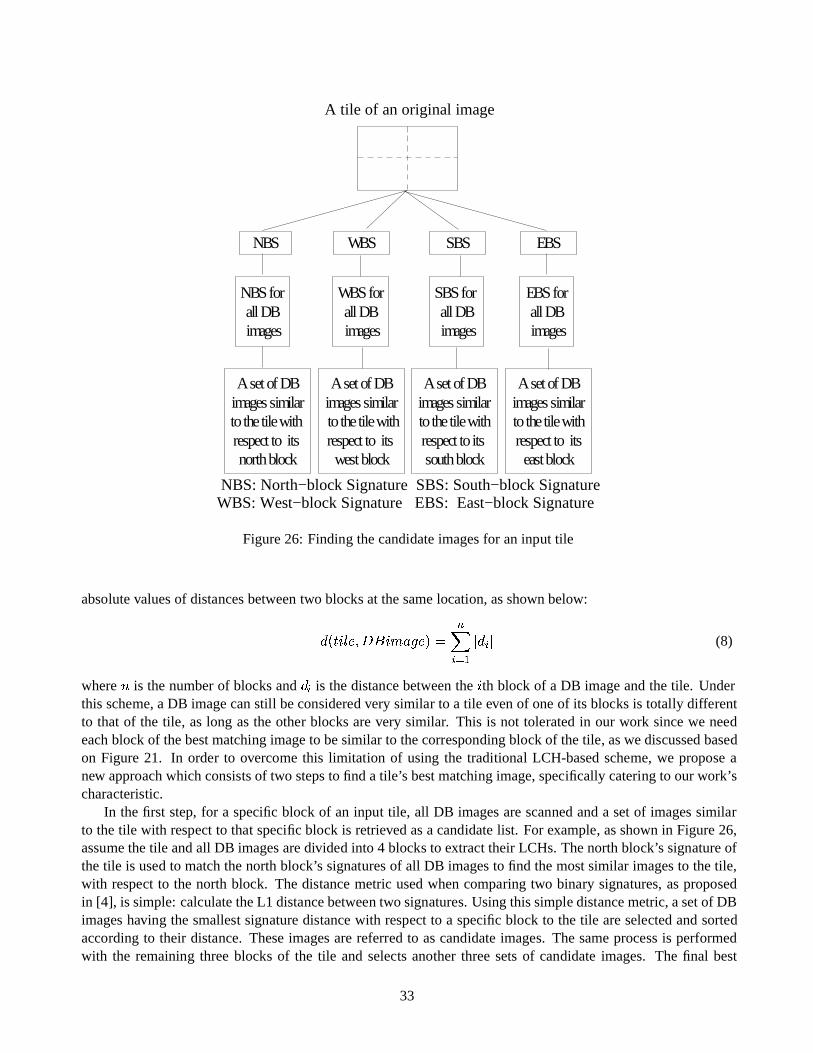
A tile of an original image
NBS: North−block Signature SBS: South−block Signature WBS: West−block Signature EBS: East−block Signature
NBS WBS SBS EBS
EBS for all DB images
SBS for all DB images
WBS for all DB images
NBS for all DB images
A set of DB images similar to the tile with respect to its south block
A set of DB images similar to the tile with respect to itseast block
A set of DB images similar
to the tile with respect to its north block
A set of DB images similar to the tile withrespect to its west block
Figure 26: Finding the candidate images for an input tile
absolute values of distances between two blocks at the same location, as shown below:
��� � � !$� ��� � � � � � � � � ��� � � � � � (8)
where � is the number of blocks and� � is the distance between the � th block of a DB image and the tile. Under
this scheme, a DB image can still be considered very similar to a tile even of one of its blocks is totally differentto that of the tile, as long as the other blocks are very similar. This is not tolerated in our work since we needeach block of the best matching image to be similar to the corresponding block of the tile, as we discussed basedon Figure 21. In order to overcome this limitation of using the traditional LCH-based scheme, we propose anew approach which consists of two steps to find a tile’s best matching image, specifically catering to our work’scharacteristic.
In the first step, for a specific block of an input tile, all DB images are scanned and a set of images similarto the tile with respect to that specific block is retrieved as a candidate list. For example, as shown in Figure 26,assume the tile and all DB images are divided into 4 blocks to extract their LCHs. The north block’s signature ofthe tile is used to match the north block’s signatures of all DB images to find the most similar images to the tile,with respect to the north block. The distance metric used when comparing two binary signatures, as proposedin [4], is simple: calculate the L1 distance between two signatures. Using this simple distance metric, a set of DBimages having the smallest signature distance with respect to a specific block to the tile are selected and sortedaccording to their distance. These images are referred to as candidate images. The same process is performedwith the remaining three blocks of the tile and selects another three sets of candidate images. The final best
33

North list West list South list East listImage Name (distance)
C (2) C (3) D (3) B (6)B (5) E (6) A (7) F (7)A (6) F (9) E (8) A (9)
Table 9: 4 candidates lists.
matching image for the input tile is selected only from these candidate images. The size of the candidate imagelist for each block is a parameter used in our system. It controls the number of candidate images and thus reflectsthe degree to which we allow a block of a DB image to be dissimilar to its corresponding block of the input tile.The effect on processing time and the quality of the target image mosaic of this parameter is discussed in detailin Chapter 4.
After obtaining all candidate images, we propose two schemes to select the best matching image among themin the second step.
Most Often Selecting Scheme (MOSS)
Obviously, if the same image appears in first place in all candidate image lists, that is a perfect matchingimage for the input tile. This gives us the idea that we can select the image appearing most often in all lists. Wedefine the MOSS similarity between a candidate image and a tile as shown in Equation 9:
����� � � � � � !$� ��� � � � � � � ��� � � ��� � � � (9)
where � is the number of the candidate image list,� � �
if the candidate image appears in the � th list, and� � � if the candidate image does not appear. We then select the image with the greatest MOSS similarity as
the best matching image. For example, candidate image lists for each of 4 blocks of an input tile are shown inTable 9. The MOSS similarity between each candidate image and the input tile is shown in Table 10. As we cansee, image A has the greatest MOSS similarity since it appears 3 times in 4 lists, which is the most among allcandidate images. Thus, it is selected as the best matching image for the tile. The idea behind this approach isthat the more times a DB image appears in candidate lists, the more blocks of this image are similar to the tile,thus the more this image matches the tile.
Candidate MOSS similarity Candidate MOSS similarityA 1+0+1+1=3 D 0+0+1+0=1B 1+0+0+1=2 E 0+1+1+0=2C 1+1+0+0=2 F 0+1+0+1=2
Table 10: MOSS similarity between candidate images and an input tile
34
Candidate DOSS Similarity Candidate DOSS Similarity
A�& �
�' �
�* � � �
D�& � � �
B�+ �
�& � � � �
E�& �
�( � � ��
C�� �
� � � ���F
�* �
�' � � ��
Table 11: DOSS similarity between candidate images and an input tile
Distance and Occurrence Selecting Scheme (DOSS)
In addition to selecting the image appearing the greatest number of times in all candidate lists as the bestmatching image, we try another approach which also considers the actual distance between blocks of a DB imageand a tile. As we can see in Table 9, all candidate images in each list are sorted according to their distance tothe same block of the tile. We define the DOSS similarity between a candidate image and a tile as shown inEquation 10:
��� � � � � � �.! � ��� � � � � � � ��� � � ��� �
� � (10)
where � is the number of times the candidate image appears in all candidate lists, and� � is the distance
between the candidate image and the tile in list � . We then select the image with the greatest DOSS similarity asthe best matching image. The idea behind this approach is that the more often an image appears in the candidatelist, the more similar it is to the input tile; at the same time, the smaller distance it has to the input tile with respectto each block, the more similar it is to the tile. However, different from MOSS, DOSS emphasis more on thesmall distance that a candidate image may have. That is, if two candidate images appears the same number oftimes in candidate lists and have the same total distance, the image with a very small distance in any candidatelist is considered as the best matching image. In addition, since the DOSS is used based on candidate lists, theabsence of an image in any candidate has to be considered. That is why instead of using the total distance, thereciprocal of the distance is used. We consider the similarity between an image which is not present in a candidatelist and a tile to be 0. The DOSS similarities between all candidate images and an input tile are shown in Table 11.As we can see, image C is considered as the best matching image under this selecting scheme. Calculating thesimilarity between a candidate image and an input tile in this way, we consider not only the number of times acandidate image appears in all lists, but also its actual distance to the tile. How to decide the best matching imageamong all candidate DB images is also a parameter used in our system. A discussion of this parameter, with itsexperimental results is presented in Chapter 4.
3.3 Implementation Issue - Using Cache
In our work, an original image is divided into thousands of tiles, and each of these tiles is processed by the systemto find its best matching image, which is a time-consuming process. Based on the analysis of our work, whenan image is divided into many tiles, some of these tiles may have the exact same colour content, especially forimages having a large area with the same background colours. Given the idea that tiles having the exact samecolour content have the same best matching image, we try to avoid processing such tiles repeatedly, in order tospeed up the process of generating an image mosaic. A caching technique is used in our system for this purpose.When the system begins processing an input tile, it goes to a cache to find whether there is any candidate tilealready in the cache which has the exact same colour content as the input tile, based on their binary signatures. Ifthe system finds one, then the input tile is considered as having the same best matching image with that candidatetile. If not, the system processes the input tile, finds its best matching image, and stores binary signatures of theinput tile, as well as its best matching image, into the cache. This process goes through each and every tile of
35

an original image during the process of generating an image mosaic. By making use of a cache, the system doesnot need to repeatedly scan the whole image database to find the best matching image for tiles having the samecolour content, which saves a considerable amount of processing time. Some experimental results of using cacheare given in Chapter 4.
4 Experimental Results
In this chapter, different image mosaics generated by our system are evaluated according to different parame-ters used in the generating process. Processing time and the quality of target image mosaics are the two maincharacteristics we are concerned with.
4.1 Experimental Setup
As mentioned earlier, our Mosaicture methodology is designed and implemented as an image mosaic generatingsystem. C, C-Shell script, and ImageMagic API4 are used to implement the system under Linux OS. All theimage mosaics in our experiments are generated using a PC with a 550MHz Celeron CPU and 128 Mbytes mainmemory.
Instead of using just one or two test images, we use a test image set consisting of 33 different images toperform the experiments, and their average result values are used for analysis. These 33 colour images areselected from the “Corel GALLERY 1,000,000” CDROM. They have different semantic content and colourdistributions. For instance, some of them have a large background area with a single colour, while others havecomplex colour distributions. In addition, they are all of the same dimension, which ensures that the processingtime and image mosaic’s quality is dependent only on the different parameters being used. In our experiments,33 images are used as original images, based on which image mosaic reproductions are generated. As well,the image database used in our system is pre-processed to guarantee that all DB images also have the samedimension.
As an image mosaic generating system, the processing time for generating an image mosaic, as well as itsquality, are two main concerns. Typically, a better system generates an image mosaic with higher quality usingless processing time. In our system, different parameters are used to control an image mosaic generating process,which consequently affects the processing time and the quality. There are 5 parameters used in our system:1. The size of the image database2. The number of quantization colours3. The scheme used to divide an image to get its LCHs4. The number of candidate images in each candidate list5. The approach used to select the best matching image from candidate lists
Different values or approaches of these 5 parameters are selected and used in an image mosaic generatingprocess. When we evaluate the effect of a specific parameter, we keep other parameters at a default value. Thepossible choices and default values for each parameter can be seen in Table 12. The experimental result andanalysis for each value of each parameter are discussed in detail in section 4.3.
4.2 Distance Measure
It is simple to evaluate the processing time of an image mosaic generating process using different parametervalues. On the contrary, the quality of an image mosaic is difficult to evaluate in a quantitative way, since noappropriate algorithm currently exists. However, in our work, we experiment with some ideas for evaluating an
4http://www.imagemagick.org
36

Parameter Possible Values Default Value
(1) 33856, 13846 33856(2) 8, 27, 64 64(3) 4(N, W, S, E), 5(N, W, S, E, C) 4(N, W, S, E)(4) 3, 5, 10, 30, 50 30(5) DOSS similarity, MOSS similarity MOSS similarity
Table 12: Parameters and their default values used in our system
Image Pixel 1(0, 0) Pixel 2(0, 1) Pixel 3(1, 0) Pixel 4(1, 1)
Original Image (23, 45, 213) (5, 212, 37) (145, 48, 57) (219, 3, 4)
Image A (34, 67, 187) (15, 190, 42) (196, 34, 66) (198, 6, 12)Image B (123, 245, 13) (38, 124, 231) (45, 32, 189) (23, 46, 165)
Table 13: Pixel values of an original image and its two image mosaics
image mosaic’s quality in a quantitative way. Since an image mosaic is generated as a reproduction of an originalimage, the more similar an image mosaic is to its original image, the better the image mosaic is. So, in ourwork, we use the distance between an image mosaic and its original image as a criterion to evaluate the mosaic’squality. The smaller distance an image mosaic has from its original image, the better the image mosaic is. Thereare many approaches for calculating the distance between two images, as discussed in Chapter 3. We select twoof them, as well as propose a new approach to calculate the distance between an image mosaic and its originalimage in order to evaluate the image mosaic’s quality.
Average Pixel-to-Pixel Distance (APP Distance)
Comparing two images based on their pixels is simple to understand and implement. Under the APP Distancemeasure, the distance between two images, A and B, which are the same size, is calculated as the average colourdifference at a pixel, as shown in Equation 11:
����� � ��� � � ����� �,� � � � � ������ �,� � - � - ��� � � ����� �,�� � � ����� �,�! � � � � � ����� � �� � � ����� �,�! � � � � � ����� � �� � ������ � �! � �
�� � (11)
where�� � � � is the coordinate of a pixel, �
� � is the total pixel number for both images, and� ����� � �� is the value
of primary colour R of the pixel with the coordinate�� � � � of image A. According to this distance measure, each
pair of pixels at the same location of two images is compared according to the colour value of each of threeprimary colours. The average distance of all pairs of pixels is deemed as the distance between two real images.For example, an original image and its two image mosaics are shown in Table 13, presented in the format of pixelcolour values. All three images have 4 pixels, and the APP Distances between the original image and the othertwo image mosaics, according to Equation 11, are shown in Equation 12. As we can see, image A has a smallerAPP Distance to the original image and thus is considered as a better image mosaic. This distance measure isbased on the spatial distribution of images when calculating their distance. The colour distribution of images isnot taken into consideration.
��� � � � � � � ��! � � # � � � � � � � ��� � ��� � � � � � � ��! � � # � � � � ��� � ���� � ���
(12)
37
GCH Distance
Different from the APP Distance measure, the GCH Distance scheme takes the colour distribution of imagesinto consideration. As discussed in Chapter 2, GCH represents the global colour distribution of an image bycounting and normalizing how many pixels belong to each colour. In our work, we choose to use the L2 distancebetween two GCHs to represent the distance between two images, as shown in Equation 13.
����� � ��� � �������� ��� � �� � � !� � � (13)
where � is the number of quantization colours, and� �� is the colour histogram for th colour in image A. For
example, GCHs for an original image O and its two image mosaics under 4 quantization colours, A and B, areshown below:
� � � � � � ��� � ��� � � �"��� � �� � � � � �� �"� � ��� � � ��� �� �� ! � � � � � ��� �� �"� � ��� �� �According to the L2 distance measure that we discussed in Chapter 2, the distance between the original imageand its image mosaics are: ��� � � � � � � ���
��� � � ��� � � �!(14)
As we can see, A is considered as a better image mosaic since it has a smaller GCH distance to the originalimage.
Multi-level Colour Histogram Distance (MLCH Distance)
An image mosaic has an intended visual effect. The content of the whole image comes out clearly only whenit is looked at from many steps away. Due to this characteristic of image mosaics, we propose a new approachfor evaluating an image mosaic’s quality. This approach is based on LCH distance, while considering the specialcharacteristics of image mosaics. The basic idea is the following: when two image mosaics are looked at from faraway, their difference probably cannot be seen clearly, but when they are looked at from a closer distance, theirdifference is more clear. I.e., the closer we are to two image mosaics, the more difference we can see betweenthem. What we do in our MLCH Distance measure is the following: we first calculate the GCH distance betweenthe images according to Equation 13, we then tile both images and obtain their average LCH distance. Finally, weuse the difference between these two distances as the distance between the original image and its image mosaic.The smaller this distance is, the better an image mosaic is. The idea behind this approach is that the better animage mosaic is, the smaller difference there is between looking at the image from different distances. In ourwork, we tile an image mosaic, as well as its original image, into 5x5 blocks to get the average LCH distance,as shown in Figure 27. Finally, we use the difference between the GCH distance and the average LCH distanceunder 5x5 blocks as the final distance. Equation 15 shows how we calculate the distance between an originalimage and its image mosaic A.
���� #�� � � � � � � � � #�� � � � � � � ��� #�� � � � � � (15)
where�� #�� � � � � � is shown below:
�� #�� � � � � � � ��� � �� � � � ��� � � � �� � � � � � !� � � � � �
�� ! (16)
38

Figure 27: The left-hand image is tiled into 5x5 blocks to extract LCHs
where � and ! are the block numbers of an image being divided into on length and on width, respectively, � is thenumber of quantization colours; and
� �� � � � is the colour histogram for th colour in � th block of image A.For example, the GCHs as well as the LCHs under 2x2 blocks of an original image, and its image mosaic
under 4 quantization colours, are shown in Table 14. According to Equation 13, the GCH distance between theoriginal image and image mosaic A is:
��� #�� � � � � � � � ��As well, according to Equation 16, the average LCH distance between them is:
�� #�� � � � � � � � � ��
Then according to Equation 15, the MLCH Distance between the original image and image mosaic A is:
���� #�� � � � � � � � � �� � � �� � � ���
Three distance measures have been discussed up till now in this section. We choose APP and GCH distancemeasures, since they consider the spatial distribution and colour distribution of images, respectively. The newMLCH distance measure we proposed is based on human perception of images. According to these distancemeasures, the smaller the distance an image mosaic has to its original image, the better the image mosaic is.Image mosaics’ quality will be analyzed based on these three distance measures. In addition, an analysis of ournew distance measure is given in section 4.4.2.
4.3 Experimental results and analysis
In this section, all experimental results are given and analyzed. When generating an image mosaic, we divide theoriginal image into
��� � ���tiles, which guarantees that the dimension of each tile is the same as the DB images,
Colour Histogram Original Image Image Mosaic A
GCH�20%, 30%, 15%, 35% � �
10%, 25%, 35%, 30% �Block 1’s LCH
�30%, 10%, 20%, 40% � �
10%, 20%, 20%, 50% �Block 2’s LCH
�20%, 10%, 20%, 50% � �
5%, 30%, 20%, 45% �Block 3’s LCH
�15%, 40%, 10%, 35% � �
15%, 45%, 40%, 0% �Block 4’s LCH
�15%, 60%, 10%, 15% � �
10%, 5%, 60%, 25% �Table 14: GCHs and LCHs for an original image and its image mosaic
39
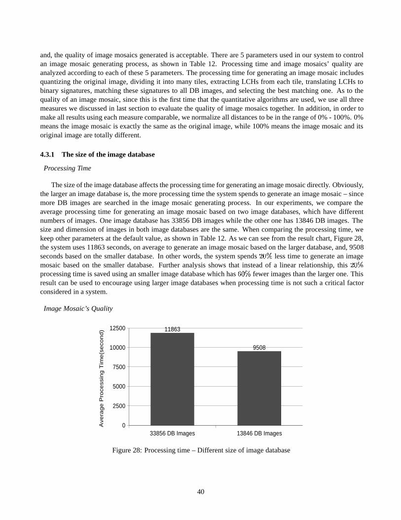
and, the quality of image mosaics generated is acceptable. There are 5 parameters used in our system to controlan image mosaic generating process, as shown in Table 12. Processing time and image mosaics’ quality areanalyzed according to each of these 5 parameters. The processing time for generating an image mosaic includesquantizing the original image, dividing it into many tiles, extracting LCHs from each tile, translating LCHs tobinary signatures, matching these signatures to all DB images, and selecting the best matching one. As to thequality of an image mosaic, since this is the first time that the quantitative algorithms are used, we use all threemeasures we discussed in last section to evaluate the quality of image mosaics together. In addition, in order tomake all results using each measure comparable, we normalize all distances to be in the range of 0% - 100%. 0%means the image mosaic is exactly the same as the original image, while 100% means the image mosaic and itsoriginal image are totally different.
4.3.1 The size of the image database
Processing Time
The size of the image database affects the processing time for generating an image mosaic directly. Obviously,the larger an image database is, the more processing time the system spends to generate an image mosaic – sincemore DB images are searched in the image mosaic generating process. In our experiments, we compare theaverage processing time for generating an image mosaic based on two image databases, which have differentnumbers of images. One image database has 33856 DB images while the other one has 13846 DB images. Thesize and dimension of images in both image databases are the same. When comparing the processing time, wekeep other parameters at the default value, as shown in Table 12. As we can see from the result chart, Figure 28,the system uses 11863 seconds, on average to generate an image mosaic based on the larger database, and, 9508seconds based on the smaller database. In other words, the system spends
� ��less time to generate an image
mosaic based on the smaller database. Further analysis shows that instead of a linear relationship, this � ��
processing time is saved using an smaller image database which has�� ��
fewer images than the larger one. Thisresult can be used to encourage using larger image databases when processing time is not such a critical factorconsidered in a system.
Image Mosaic’s Quality
33856 DB Images 13846 DB Images0
2500
5000
7500
10000
12500 11863
9508
Ave
rag
e P
roce
ssin
g T
ime
(se
con
d)
Figure 28: Processing time – Different size of image database
40

When an image mosaic is being generated, its original image is first divided into many tiles. For each tile,the system searches the image database and selects the best matching image for it, based on its binary signatures.Basically, the more DB images we have, the better the DB images similar to the tile that can be selected into thecandidate list, thus the better “best matching” image we can find for the tile. Figure 29 shows the experimentalresults. The average distance between 33 image mosaics and their original images under 3 distance measures –APP Distance, GCH Distance, and MLCH Distance – are put together in one figure. As we can see, under alldistance measures, image mosaics generated based on the larger database have smaller distances to their originalimages. In particular, for images with a large area of a single colour, many divided tiles have the same colourcontent. If a DB image having the most similar colour content to these tiles only appears in the larger imagedatabase, the quality of the target image mosaic based on this larger image database will obviously be better.
APP Distance GCH Distance MLCH Distance
Difference 1.41% 5% 1.43%
Table 15: Difference between image mosaic’s quality using 3 different distance measures
APP Distance GCH Distance MLCH Distance0.00%
2.00%
4.00%
6.00%
8.00%
10.00% 9.96%
6.43%
2.86%
11.37% 11.43%
4.29%
33856 DB Images 13846 DB Images
Dis
tanc
e to
the
orig
inal
imag
e
Figure 29: Quality comparison – Different size of image database
Figure 30: The right-hand mosaic which is generated using the bigger imageDB is better but not so obviously
41

However, the difference between the image mosaics’ quality based on the different size of the image databasesis small, as shown in Table 15. Since an image mosaic’s quality is evaluated according to its similarity to theoriginal image, the absolute difference between two image mosaics’ normalized distance to the original image isregarded as the difference between their quality. As we can see from Table 15, the greatest difference betweenimage mosaics’ quality is
� �under GCH Distance, while it is only around
�� � �under other distance measures.
Figure 30 shows two such image mosaics generated based on different number of DB images. We cannot easilytell which one is definitely better, even though we can see that there is some more noise on the left one. Inaddition, the image mosaics generated using the smaller database still have a similar visual content to the originalimages according to human perception. This result tells us that an image database having 13846 images is largeenough. In comparison with the difference in processing time, which is
� ��between the larger and the smaller
image database, we believe the smaller image database contains enough DB images to generate a good imagemosaic. Anyway, if the quality of image mosaics is the main concern of users, large image databases can be usedto generate better image mosaics, due to the non-linear relationship between DB image numbers and processingtime.
4.3.2 The number of quantization colours
The number of quantization colours determines how much colour information about an image is encoded in itsmetadata. Basically, the greater the number of colours an image is quantized to, the less colour information islost. For example, when the quantization colour is 64, that means there are 4 different colour levels in each ofthree primary colours under the uniform quantization scheme. When the quantization colours are set to 8, thereare only 2 different colour levels left. When more colour information is stored in the metadata, more storage isused and more time is needed to compare this information with other data. The storage for binary signatures ofan image using different number of quantization colours is shown in Table 16.
Quantization Colours Storage Requirement for an image
64��� � � � �
bits = 128 bytes27
�� ��� �bits = 54 bytes
8�� � � �
bits = 16 bytesThe image is divided into 4 blocks to get LCHs
4 bits are used for each colour in an image’s binary signature
Table 16: Storage for an image’s metadata using different colours
Processing Time
Since more colour information is encoded in the metadata of DB images, as well as an original image, usinga higher number of quantization colours, more work is needed to compare these metadata. Figure 31 shows theaverage processing time for generating image mosaics for 33 test images using different quantization colours. Aswe can see, the more quantization colours used, the more time the system spends to generate an image mosaic.Note that, the difference between processing times using different quantization colours is very dramatic. Forinstance, generating an image mosaic using 27 quantization colours saves
�� �processing time in comparison
with the same process using 64 colours. The result tells us that the processing time for generating an imagemosaic is heavily dependent on the number of quantization colours used.
Image Mosaic’s Quality
42
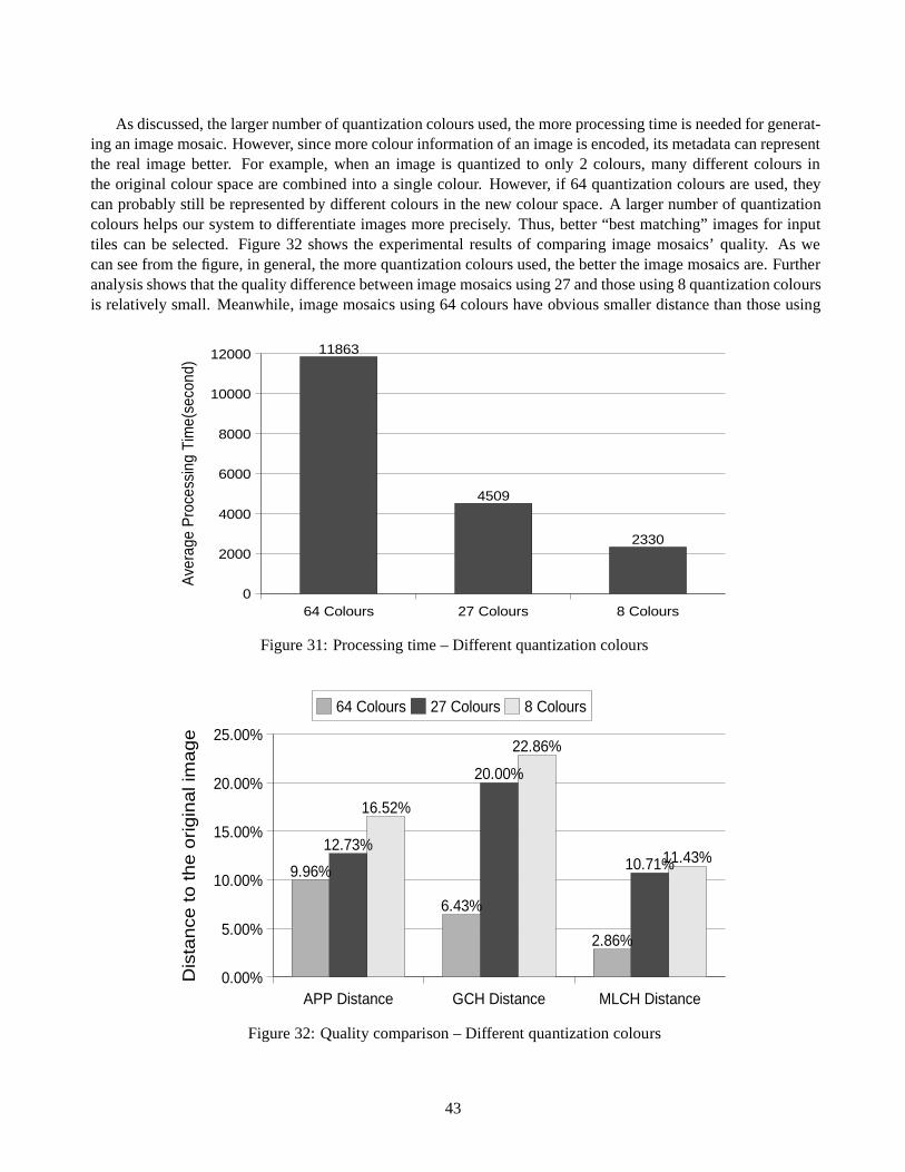
As discussed, the larger number of quantization colours used, the more processing time is needed for generat-ing an image mosaic. However, since more colour information of an image is encoded, its metadata can representthe real image better. For example, when an image is quantized to only 2 colours, many different colours inthe original colour space are combined into a single colour. However, if 64 quantization colours are used, theycan probably still be represented by different colours in the new colour space. A larger number of quantizationcolours helps our system to differentiate images more precisely. Thus, better “best matching” images for inputtiles can be selected. Figure 32 shows the experimental results of comparing image mosaics’ quality. As wecan see from the figure, in general, the more quantization colours used, the better the image mosaics are. Furtheranalysis shows that the quality difference between image mosaics using 27 and those using 8 quantization coloursis relatively small. Meanwhile, image mosaics using 64 colours have obvious smaller distance than those using
64 Colours 27 Colours 8 Colours0
2000
4000
6000
8000
10000
12000 11863
4509
2330
Ave
rage
Pro
cess
ing
Tim
e(se
cond
)
Figure 31: Processing time – Different quantization colours
APP Distance GCH Distance MLCH Distance0.00%
5.00%
10.00%
15.00%
20.00%
25.00%
9.96%
6.43%
2.86%
12.73%
20.00%
10.71%
16.52%
22.86%
11.43%
64 Colours 27 Colours 8 Colours
Dis
tan
ce t
o t
he
ori
gin
al i
ma
ge
Figure 32: Quality comparison – Different quantization colours
43
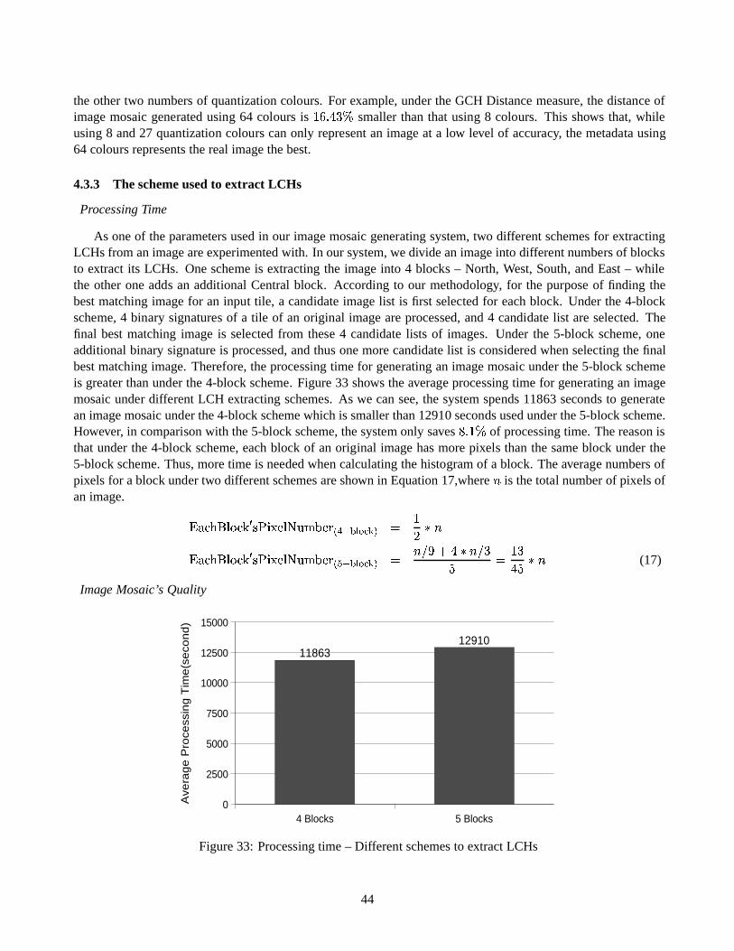
the other two numbers of quantization colours. For example, under the GCH Distance measure, the distance ofimage mosaic generated using 64 colours is
�� � � � �smaller than that using 8 colours. This shows that, while
using 8 and 27 quantization colours can only represent an image at a low level of accuracy, the metadata using64 colours represents the real image the best.
4.3.3 The scheme used to extract LCHs
Processing Time
As one of the parameters used in our image mosaic generating system, two different schemes for extractingLCHs from an image are experimented with. In our system, we divide an image into different numbers of blocksto extract its LCHs. One scheme is extracting the image into 4 blocks – North, West, South, and East – whilethe other one adds an additional Central block. According to our methodology, for the purpose of finding thebest matching image for an input tile, a candidate image list is first selected for each block. Under the 4-blockscheme, 4 binary signatures of a tile of an original image are processed, and 4 candidate list are selected. Thefinal best matching image is selected from these 4 candidate lists of images. Under the 5-block scheme, oneadditional binary signature is processed, and thus one more candidate list is considered when selecting the finalbest matching image. Therefore, the processing time for generating an image mosaic under the 5-block schemeis greater than under the 4-block scheme. Figure 33 shows the average processing time for generating an imagemosaic under different LCH extracting schemes. As we can see, the system spends 11863 seconds to generatean image mosaic under the 4-block scheme which is smaller than 12910 seconds used under the 5-block scheme.However, in comparison with the 5-block scheme, the system only saves
� � �of processing time. The reason is
that under the 4-block scheme, each block of an original image has more pixels than the same block under the5-block scheme. Thus, more time is needed when calculating the histogram of a block. The average numbers ofpixels for a block under two different schemes are shown in Equation 17,where � is the total number of pixels ofan image.
����������� ������������� ������ �"!#�%$ � ) � &('*),+.- � � � ������������ ��� � ������� ������ �"!#�%$ � + � &('*),+.- � � ��� � �
� � ��� �� � �� � � � (17)
Image Mosaic’s Quality
4 Blocks 5 Blocks0
2500
5000
7500
10000
12500
15000
1186312910
Ave
rag
e P
roce
ssin
g T
ime
(se
con
d)
Figure 33: Processing time – Different schemes to extract LCHs
44

APP Distance GCH Distance MLCH Distance0.00%
2.00%
4.00%
6.00%
8.00%
10.00% 9.96%
6.43%
2.86%
10.04%
5.71%
2.14%
4−block 5−block
Dis
tanc
e to
the
orig
inal
imag
e
Figure 34: Quality comparison – Different schemes to extract LCHs
In CBIR systems, different schemes used to divide an image into blocks in order to extract LCHs affects theresult of an image retrieval process. Typically, the greater the number of blocks an image is divided into, the moreimage information is encoded into the metadata, thus the better the result of image retrieval is. According to this,using the 5-block scheme to extract images’ LCHs should also help the system to generate better image mosaicsthan use of the 4-block scheme. This is true, as shown in Figure 34. Under GCH and MLCH distance measures,using the 5-block scheme is better. However, the difference shown in the result is small. Also, under the APPDistance, the image mosaic generated under the 4-block scheme is even a little bit better than that achieved byusing the 5-block scheme. The reason is that finding a good best matching image for each tile is not the onlyfactor that determines the quality of the final image mosaic. In our system, hundreds or thousands of images areput together to build up an image mosaic. So, the relationship between adjacent images is as well important.Typically, a good image mosaic requires that adjacent images have smooth colour conversions, especially at theiredges. Under the 5-block scheme, the central part of an image plays a more important role when retrieving itsbest matching image than the 4-block scheme, which may result in not so good conversions between adjacentimages. On the whole, the results show that the scheme of extracting images’ LCHs actually does not affect theimage mosaics’ quality very much in our system. However, we select the 5-block scheme as the better choicesince the image mosaics using this scheme has smaller distance under both GCH and MLCH distance measures.
4.3.4 The size of the candidate image list
Processing Time
This parameter, the size of the candidate image list, also affects the processing time for generating an imagemosaic. Figure 35 shows the experimental results. As we can see, the more images a candidate list has, the moreprocessing time is needed to generate an image mosaic. According to our methodology, a bigger list size meansmore DB images are selected as candidate images for an input tile, which in turn costs more processing time.Besides, the system also needs more time to calculate the distance of each image in the candidate lists in order toselect the best matching image. Since the processing time of these two procedures in our system are affected bythe size of the candidate image list in the way we discussed, the bigger a candidate list is, the more processingtime is needed to generate an image mosaic.
45
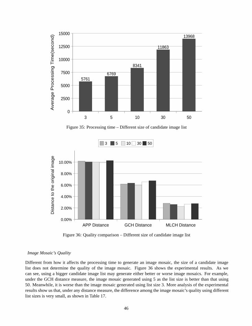
3 5 10 30 500
2500
5000
7500
10000
12500
15000
57616769
8341
11863
13968
Ave
rag
e P
roce
ssin
g T
ime
(se
con
d)
Figure 35: Processing time – Different size of candidate image list
APP Distance GCH Distance MLCH Distance0.00%
2.00%
4.00%
6.00%
8.00%
10.00%
3 5 10 30 50
Dis
tan
ce t
o t
he
orig
ina
l im
ag
e
Figure 36: Quality comparison – Different size of candidate image list
Image Mosaic’s Quality
Different from how it affects the processing time to generate an image mosaic, the size of a candidate imagelist does not determine the quality of the image mosaic. Figure 36 shows the experimental results. As wecan see, using a bigger candidate image list may generate either better or worse image mosaics. For example,under the GCH distance measure, the image mosaic generated using 5 as the list size is better than that using50. Meanwhile, it is worse than the image mosaic generated using list size 3. More analysis of the experimentalresults show us that, under any distance measure, the difference among the image mosaic’s quality using differentlist sizes is very small, as shown in Table 17.
46

APP Distance GCH Distance MLCH Distance
Biggest Difference 0.39% 0.78% 0.55%
Table 17: Difference among image mosaics using different list sizes
The reason behind this is that the best matching image selected for a tile is not definitely better when moreimages are selected into each candidate list. For example, suppose we use the MOSS similarity to select the bestmatching image among 4 candidate image lists. Table 18 shows the four lists when the size is set to 3. As we cansee, candidate image A appears twice, which is the most often among all candidate images, so it is selected to bethe best matching image for the input tile.
Now we set the list size to 50. If the candidate images are selected as shown in Table 19, then candidateimage L is selected as the best matching image. As we can see, image L appears 3 times in all four lists and inaddition, the positions of it are all very near the top of the lists. In this case, we believe image L is more similarto the input tile than image A. However, if the candidate images are selected as shown in Table 20, the result isopposite. This time, candidate image L appears at all final positions in candidate lists, which means its distanceto the input tile is great. However, it is still selected as the best matching image due to its 3 appearances on all 4candidate lists. In this case, image L is more likely not as good as image A as the best matching image for theinput tile.
In conclusion, we believe list size 3 to be the best choice since it cost the system the least processing timewithout an obvious drop in quality.
4.3.5 The approach used to select the best matching image
Processing Time
As one of our system’s parameters, the approach used to select the best matching image among candidateimage lists does not affect the processing time at all. Figure 37 shows the experimental results. As we can see, theaverage processing time for generating an image mosaic using different approach for selecting the best matchingimage is almost the same. The reason is that, unlike other parameters, the only process affected by this parameterare memory operations which are performed after all the candidate images are selected. Therefore, the processingtime changes little, if at all, when different approach of this parameter is used.
North List West List South List East List
1 B D G I2 C E H J3 A F A K
Table 18: Candidate image lists with size 3
47

North List West List South List East List
1 B D G I2 C E H J3 A F A K4 L L L M. . . . .. . . . .
50 . . . .
Table 19: A good example of setting list size to 50
North List West List South List East List
1 B D G I2 C E H J3 A F A K. . . . .. . . . .. . . . .
50 L L L M
Table 20: A bad example of setting list size to 50
MOSS DOSS0
2500
5000
7500
10000
12500 11863 11744
Ave
rage
Pro
cess
ing
Tim
e (S
econ
d)
Figure 37: Processing time – Different best matching image selection
Image Mosaic’s Quality
Even though it does not affect the processing time, the approach used to select the best matching image doesindeed affect the quality of the image mosaic. As discussed in Chapter 3, there are two approaches used in oursystem: MOSS, which selects the image with most occurrences in all candidate lists as the best matching image;and DOSS, which takes the distance of candidate images into consideration. Figure 38 shows the experimentalresults. As we can see, the image mosaic generated using MOSS always has a smaller distance to the originalimage. This shows that more blocks of an image being similar to a tile is more important than the smaller total
48

APP Distance GCH Distance MLCH Distance0.00%
2.50%
5.00%
7.50%
10.00%
12.50%
9.96%
6.43%
2.86%
11.15%10.21%
3.71%
MOSS DOSS
Dis
tanc
e to
the
orig
inal
imag
e
Figure 38: Quality comparison – Different best matching image selection
distance of it to the tile. In other words, an image with more blocks similar to a tile should be selected as the bestmatching image rather than the one with fewer similar blocks, but having a smaller total distance.
5 Conclusion
5.0.6 The effects of five parameters
Our image mosaic generating system has been experimented according to the parameters used. After analyzingthe experimental results, we know that each of these 5 parameters affects the processing time and the qualityof an image mosaic to some degree. However, different parameters play different roles in the system. Forexample, with respect to the processing time, the number of quantization colours affects the system the most,while the approach of selecting the best matching image among candidate images does not play an importantrole. The degree of effect on the processing time and image mosaics’ quality of different parameters are shownin Tables 21 and 22.
Parameters Effect on Processing Time
Quantization Colours GreatestSize of Candidate List Second
Size of Image DB ThirdLCH Extraction Small
Best Matching Image Selection Small
Table 21: The effect of different parameters on processing time
In addition, according to our analysis of the results, the best choice of values or approaches we tested foreach parameter can be made considering the processing time and image mosaic’s quality together. For example,even though using 64 quantization colours costs the system more processing time to generate an image mosaic,
49

Parameters Effect on image mosaic’s qualityQuantization Colours Greatest
Size of Image DB SecondBest Matching Image Selection Third
LCH Extraction SmallSize of Candidate List Small
Table 22: The effect of different parameters on image mosaic’s quality
Parameters Best Value or ApproachQuantization Colours 64 Colours
Size of Image DB 13846 DB ImagesBest Matching Image Selection MOSS Similarity
LCH Extraction Extract to 5 blocksSize of Candidate List 3
Table 23: The best value or approach for each parameter
we still believe that it is the best choice among all quantization colours tested, because of the improvement inthe image mosaic’s quality. The best choice for each parameter selected by us is shown in Table 23. However,according to different focuses of different image mosaic generating systems, other values or approaches may beselected as the best choice catering the system’s need.
5.0.7 Analysis of MLCH measure
5
10
15
20
25
30
35
1x12x2 3x3 4x4 5x5 6x6 7x7 8x8 9x9 10x10
Dis
tanc
e to
orig
inal
imag
es[%
]
Tiling levels an image being tiled to extract LCHs
64 Colours27 Colours
Figure 39: LCH distance of image mosaics using 27 and 64 quantization colours at different LCH extractinglevel
Since this is the first time that quantitative measures are used to evaluate the quality of image mosaics, we
50
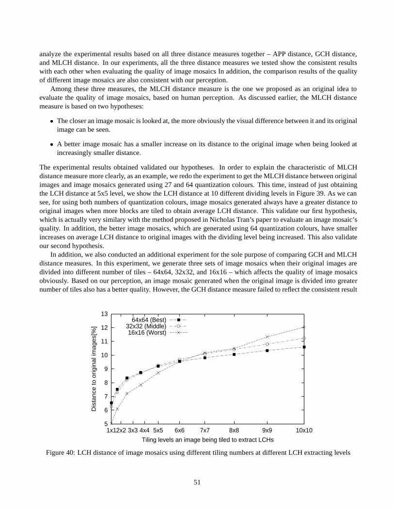
analyze the experimental results based on all three distance measures together – APP distance, GCH distance,and MLCH distance. In our experiments, all the three distance measures we tested show the consistent resultswith each other when evaluating the quality of image mosaics In addition, the comparison results of the qualityof different image mosaics are also consistent with our perception.
Among these three measures, the MLCH distance measure is the one we proposed as an original idea toevaluate the quality of image mosaics, based on human perception. As discussed earlier, the MLCH distancemeasure is based on two hypotheses:
� The closer an image mosaic is looked at, the more obviously the visual difference between it and its originalimage can be seen.
� A better image mosaic has a smaller increase on its distance to the original image when being looked atincreasingly smaller distance.
The experimental results obtained validated our hypotheses. In order to explain the characteristic of MLCHdistance measure more clearly, as an example, we redo the experiment to get the MLCH distance between originalimages and image mosaics generated using 27 and 64 quantization colours. This time, instead of just obtainingthe LCH distance at 5x5 level, we show the LCH distance at 10 different dividing levels in Figure 39. As we cansee, for using both numbers of quantization colours, image mosaics generated always have a greater distance tooriginal images when more blocks are tiled to obtain average LCH distance. This validate our first hypothesis,which is actually very similary with the method proposed in Nicholas Tran’s paper to evaluate an image mosaic’squality. In addition, the better image mosaics, which are generated using 64 quantization colours, have smallerincreases on average LCH distance to original images with the dividing level being increased. This also validateour second hypothesis.
In addition, we also conducted an additional experiment for the sole purpose of comparing GCH and MLCHdistance measures. In this experiment, we generate three sets of image mosaics when their original images aredivided into different number of tiles – 64x64, 32x32, and 16x16 – which affects the quality of image mosaicsobviously. Based on our perception, an image mosaic generated when the original image is divided into greaternumber of tiles also has a better quality. However, the GCH distance measure failed to reflect the consistent result
5
6
7
8
9
10
11
12
13
1x12x2 3x3 4x4 5x5 6x6 7x7 8x8 9x9 10x10
Dis
tanc
e to
orig
inal
imag
es[%
]
Tiling levels an image being tiled to extract LCHs
64x64 (Best)32x32 (Middle)16x16 (Worst)
Figure 40: LCH distance of image mosaics using different tiling numbers at different LCH extracting levels
51
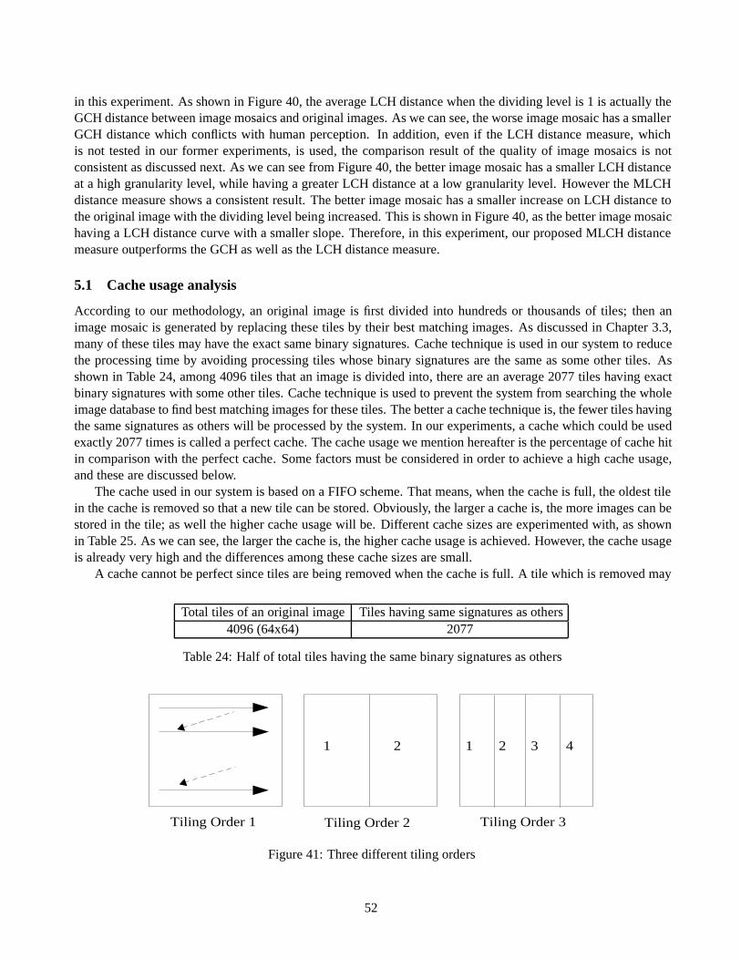
in this experiment. As shown in Figure 40, the average LCH distance when the dividing level is 1 is actually theGCH distance between image mosaics and original images. As we can see, the worse image mosaic has a smallerGCH distance which conflicts with human perception. In addition, even if the LCH distance measure, whichis not tested in our former experiments, is used, the comparison result of the quality of image mosaics is notconsistent as discussed next. As we can see from Figure 40, the better image mosaic has a smaller LCH distanceat a high granularity level, while having a greater LCH distance at a low granularity level. However the MLCHdistance measure shows a consistent result. The better image mosaic has a smaller increase on LCH distance tothe original image with the dividing level being increased. This is shown in Figure 40, as the better image mosaichaving a LCH distance curve with a smaller slope. Therefore, in this experiment, our proposed MLCH distancemeasure outperforms the GCH as well as the LCH distance measure.
5.1 Cache usage analysis
According to our methodology, an original image is first divided into hundreds or thousands of tiles; then animage mosaic is generated by replacing these tiles by their best matching images. As discussed in Chapter 3.3,many of these tiles may have the exact same binary signatures. Cache technique is used in our system to reducethe processing time by avoiding processing tiles whose binary signatures are the same as some other tiles. Asshown in Table 24, among 4096 tiles that an image is divided into, there are an average 2077 tiles having exactbinary signatures with some other tiles. Cache technique is used to prevent the system from searching the wholeimage database to find best matching images for these tiles. The better a cache technique is, the fewer tiles havingthe same signatures as others will be processed by the system. In our experiments, a cache which could be usedexactly 2077 times is called a perfect cache. The cache usage we mention hereafter is the percentage of cache hitin comparison with the perfect cache. Some factors must be considered in order to achieve a high cache usage,and these are discussed below.
The cache used in our system is based on a FIFO scheme. That means, when the cache is full, the oldest tilein the cache is removed so that a new tile can be stored. Obviously, the larger a cache is, the more images can bestored in the tile; as well the higher cache usage will be. Different cache sizes are experimented with, as shownin Table 25. As we can see, the larger the cache is, the higher cache usage is achieved. However, the cache usageis already very high and the differences among these cache sizes are small.
A cache cannot be perfect since tiles are being removed when the cache is full. A tile which is removed may
Total tiles of an original image Tiles having same signatures as others4096 (64x64) 2077
Table 24: Half of total tiles having the same binary signatures as others
Tiling Order 1 Tiling Order 2 Tiling Order 3
1 2 21 3 4
Figure 41: Three different tiling orders
52
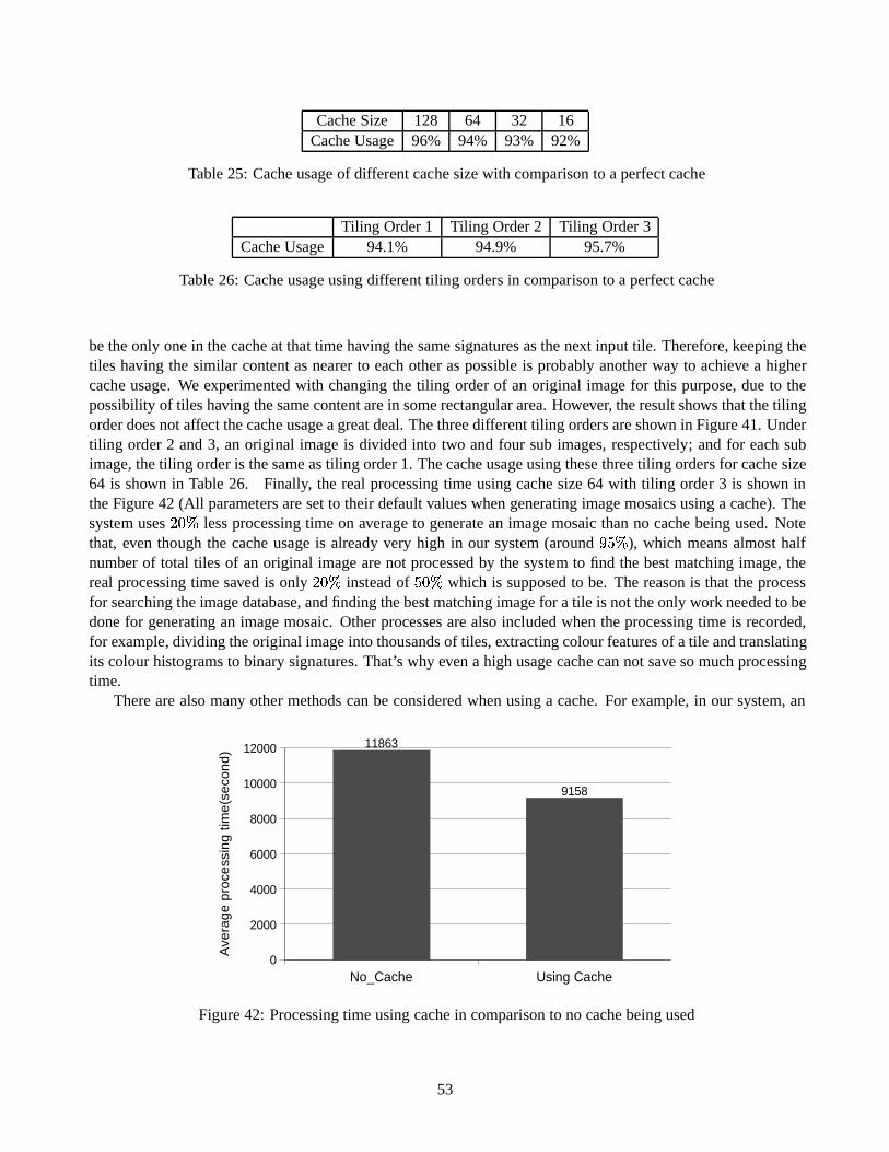
Cache Size 128 64 32 16Cache Usage 96% 94% 93% 92%
Table 25: Cache usage of different cache size with comparison to a perfect cache
Tiling Order 1 Tiling Order 2 Tiling Order 3Cache Usage 94.1% 94.9% 95.7%
Table 26: Cache usage using different tiling orders in comparison to a perfect cache
be the only one in the cache at that time having the same signatures as the next input tile. Therefore, keeping thetiles having the similar content as nearer to each other as possible is probably another way to achieve a highercache usage. We experimented with changing the tiling order of an original image for this purpose, due to thepossibility of tiles having the same content are in some rectangular area. However, the result shows that the tilingorder does not affect the cache usage a great deal. The three different tiling orders are shown in Figure 41. Undertiling order 2 and 3, an original image is divided into two and four sub images, respectively; and for each subimage, the tiling order is the same as tiling order 1. The cache usage using these three tiling orders for cache size64 is shown in Table 26. Finally, the real processing time using cache size 64 with tiling order 3 is shown inthe Figure 42 (All parameters are set to their default values when generating image mosaics using a cache). Thesystem uses
� ��less processing time on average to generate an image mosaic than no cache being used. Note
that, even though the cache usage is already very high in our system (around��� �
), which means almost halfnumber of total tiles of an original image are not processed by the system to find the best matching image, thereal processing time saved is only
� ��instead of
�� ��which is supposed to be. The reason is that the process
for searching the image database, and finding the best matching image for a tile is not the only work needed to bedone for generating an image mosaic. Other processes are also included when the processing time is recorded,for example, dividing the original image into thousands of tiles, extracting colour features of a tile and translatingits colour histograms to binary signatures. That’s why even a high usage cache can not save so much processingtime.
There are also many other methods can be considered when using a cache. For example, in our system, an
No_Cache Using Cache0
2000
4000
6000
8000
10000
12000 11863
9158
Ave
rag
e p
roce
ssin
g t
ime
(se
con
d)
Figure 42: Processing time using cache in comparison to no cache being used
53
input tile is not processed only if another tile having the exact same binary signatures exists in the cache. Moreprocessing time can be saved considering tiles with small distance as the same. However, the quality of the imagemosaic is then supposed to decrease, since different tiles use the same best matching image. The relationshipbetween an image mosaic’s quality and the degree of difference to which two tiles can be regarded having thesame best matching image is beyond the scope of this thesis and can be put in the future work.
6 Conclusion and Future work
6.1 Conclusion
The main contribution of this thesis is the design and implementation of an image mosaic generating system,which is called Mosaicture, and, the investigation of different parameters’ roles in the system. In our system, animage mosaic is generated as a reproduction of an original image. Before an image mosaic can be generated,the image database is pre-processed in order to extract the colour features of all DB images. Colour histogramsare used to represent these features, which are then translated to binary signatures. Binary signature is a kindof compact colour feature representation used in our system which saves a great deal of space when storingthe images’ metadata as well as speeding up the image searching process. When the image mosaic generatingprocess starts, the original image is first divided into many tiles. For each tile, its colour feature is extractedand represented in the same way as all the DB images. Its binary signatures are used to match metadata of allDB images to select a set of candidate images. Then, based on two different approaches we proposed, the bestmatching image for this tile is selected. The final image mosaic is generated by substituting each tile with its bestmatching image. There are many parameters used in our system to control the generating process, thus affectingthe processing time as well as the quality of image mosaics. These parameters include the number of quantizationcolours, the size of the image database, the scheme to extract images’ LCHs, the size of the candidate image list,and the approach used to select the best matching image for a tile.
Our experimental results show that each of 5 parameters plays a different role in controlling the image mosaicgenerating process. The number of quantization colours used in our system is shown to be the most importantparameter. It dramatically affects both the processing time and the quality of an image mosaic. And 64 quan-tization colours is shown to be the best choice among all the values we tested. With respect to the processingtime, the size of the candidate list and image database also play important roles. However, neither the LCHextracting scheme nor the best matching image selecting approach affects an image mosaic generating process agreat deal. With respect to the quality of an image mosaic, the size of the image database and the best matchingimage selection approach are two parameters affecting the process. In addition, considering the processing timeand image mosaic’s quality together, the best value or approach for each parameter is selected by us. Using theseparameters with their best values, our system can generate very good image mosaics similar to the original imagein acceptable time.
Another contribution of this thesis is an image mosaic evaluating measure we proposed, which is called theMLCH distance measure. This distance measure is based on human perceptions of images mosaics, which usesthe increasing speed of LCH distance as the measure to evaluate an image mosaic’s quality. The experimentalresults show that our proposed measure is the most stable one we tested, and outperforms the GCH distancemeasure.
6.2 Future Work
Our thesis focuses on the design and implementation of an image mosaic generating system. Some parametersare also experimented with to test their effects on the processing time and image mosaic’s quality. Though, thereare also some other challenging areas which may be investigated.
54

� During colour feature extracting, RGB colour space is used in our system. Other colour spaces could alsobe used such as L
�a�b and L
�u�v.
� Non-uniform colour quantization approaches could be used instead of the uniform approach used in oursystem.
� Besides 4-block and 5-block LCH extracting schemes, there are many other schemes to extract LCHs ofan image. They also can be investigated.
� Different approaches to select the best matching image for an input tile exist. More work can be done onthis topic.
� Investigation on considering different tiles to have the same best matching image can be performed so thatmore processing time can be saved.
References
[1] Mosaic magic v2.0. http://www.fishsoft.co.uk/mosaic magic.shtml.
[2] A. D. Bimbo. Visual Information Retrieval. Morgan Kaufmann Publishers, San Francisco, California, 1999.
[3] C. C. Chang and J. H. Jiang. A fast spatial retrieval using a superimposed coding technique. In Proceedingsof the International Symposium on Advanced Database Technologies and Their Integration, pages 71–78,Nera, Japan, 1994.
[4] V. Chitkara. Color-based image retrieval using compact binary signatures. Master’s thesis, ComputingScience Department, University of Alberta, 2001.
[5] C. Colombo, A. Rizzi, and I. Genovesi. Histogram families for colour-based retrieval in image databases. InProceedings 9th International Conference on Image Analysis and Processing ICIAP’97, pages (II)204–211,Firenze, Italy, September 1997.
[6] R. Echen. Art from text. http://www.rechen.f2s.com/arttext.html.
[7] E. A. El-Kwae and M. R. Kabuka. A robust framework for content-based retrieval by spatial similarity inimage databases. ACM Transactions on Information Systems (TOIS), 17:174–198, April 1999.
[8] F. Ennesser and G. Medioni. Finding waldo, or focus of attention using local color information. I.E.E.E.Transactions on Pattern Analysis and Machine Intelligence, 17:8, August 1995.
[9] P.G.B. Enser. Progress in documentation: Pictorial information retrieval. Journal of Documentation,51:126–170, 1995.
[10] A. Finkelstein and M. Range. Image mosaics. Technical Report TR-574-98, Computer Science Department,Princeton University, 1998.
[11] M. Flickner, H. Sawhney, W. Niblack, J. Ashley, Q. Huang, B. Dom, M. Gorkani, J. Hafner, D. Lee,D. Petkovic, D. Steele, and P. Yanker. Query by image content and video content: The QBIC system. IEEEComputer, pages 23–32, September 1995.
[12] R. C. Gonzalez and R. E. Woods. Digital Image Processing. Addison Wesley Publishing company, 1993.
[13] M. Hartmann. 10000 zombies. http://www.xoz.net/vs/014.html.
55

[14] W. L. Hunt. The phototiled pictures. http://home.earthlink.net/ wlhunt/index.html.
[15] P. M. Kelly, T. M. Cannon, and D. R. Hush. Query by image example: the candid approach. Storage andRetrieval for Image and Video DatabasesIII, SPIE, 2420:238–248, 1995.
[16] S. Y. Lee and M. K. Shan. Access methods of image databases. International Journal of Pattern Recognitionand Aritifical Intelligence, 4:27–44, 1990.
[17] W. Y. Ma and B. S. Manjunath. Netra: A toolbox for navigating large image databases. Multimedia systems,7:184–198, 1999.
[18] B. M. Mehtre, M. Kankanhalli, and W. F. Lee. Shape measures for content based image retrieval: Acomparison. Information Processing and Management, 33:319–337, 1997.
[19] J. Miller, G. Pass, and R. Zabih. Comparing images using colour coherence vectors. In Proceedings of the4th ACM International Conference on Multimedia, pages 65–73, Boston, Massachusetts, USA, November1996.
[20] S. Mukherjea, K. Hirata, and Y. Hara. Amore: A world wide web image retrieval engine. The WWWJournal, 2:115–132, 1999.
[21] W. Niblack, R. Barber, W. Equitz, M. Flickner, E. Glassman, D. Petkovic, and P. Yanker. The QBIC project:Querying image by content using colour, texture and shape. SPIE, 1908:115–132, February 1993.
[22] A. Pentland, R. W. Picard, and S. Sclaroff. Photobook: Content-based manipulation of image databases.International Journal of Computer Vision, 18:233–254, 1996.
[23] Y. Rubner and C. Tomasi. Texture-based image retrieval without segmentation. In Proceedings of theInternational Conference on Computer Vision, IEEE, pages 1018–1024, Kerkyra, Greece, September 1999.
[24] Y. Rui, T. S. Huang, and S. F. Chang. Image retrieval: Past present and future. Journal of Visual Communi-cation and Image Representation, 10:1–23, 1999.
[25] Y. Rui, A. She, and T. Huang. Modified fourier descriptors for shape representation - a practical approach.In Proceedings of the First International Workshop on Image Databases and Multi Media Search, pages22–23, Amsterdam, Netherlands, August 1996.
[26] S. Sclaroff, L. Taycher, and M. LaCascia. Imagerover: A content-based image browser for the world wideweb. Technical Report 1997-005, June 1997. http://citeseer.nj.nec.com/sclaroff97imagerover.html.
[27] R. Silvers. Digital composition of a mosaic image, October 2000. US Patent and Trademark Office.http://www.uspto.gov.
[28] J. Smith and S. Chang. In M. T. Maybury, editor, Intelligent Multimedia Information Retrieval, chapterQuerying by color regions using the VisualSEEk content-based visual query system. 1996.
[29] J. Smith and S. Chang. Automated binary texture feature sets for image retrieval. In Proceedings of theIEEE International Conference on Acoustics, Speech, and Signal Processing, pages 2239–2242, Atlanta,GA, USA, 1996.
[30] J. R. Smith. Integrated Spatial and Feature Image Systems: Retrieval, Compression and Analysis. Ph.d.thesis, Graduate School of Arts and Science, Columbia University, February 1997.
56
[31] J. R. Smith and S. F. Chang. Tools and techniques for color image retrieval. In Storage and Retrieval forImage and Video Databases (SPIE), pages 426–437, 1996.
[32] R. O. Stehling, M. A. Nascimento, and A. X. Falcao. On shapes of colours for content-based image retrieval.International Workshop on Multimedia Information Retrieval, November 2000.
[33] Al Stevens. Review of the book photomosaics. Electronic Review of Computer Books, 1997.
[34] M. Stricker and M. Orengo. Similarity of colour images. In Proceedings of SPIE Conference, StorageRetrieval for Still Images Video Databases, volume 2420, pages 381–392, San Jose, CA, September 1995.
[35] M. J. Swain and D. H. Ballard. Colour indexing. International Journal of computer vision, 7:11–32, 1991.
[36] K. L. Tan, B. C. Ooi, and C. Y. Yee. An evaluation of colour-spatial retrieval techniques for large imagedatabase. In Multimedia Tools and Applications. Kluwer Academic Publishers, 2001.
[37] N. Tran. Generating photomosaics: An empirical study. In Proceedings of the 1999 ACM symposium onApplied computing, pages 105–109, San Antonio, Texas, USA, 1999.
[38] L. Yang and F. Albregtsen. Fast computation of invariant geometric moments: A new method giving correctresults. In Proceeding of the International Conference on Pattern Recognition (ICPR) 94, pages 201–204,San Antonio, Texas, USA, 1994.
57
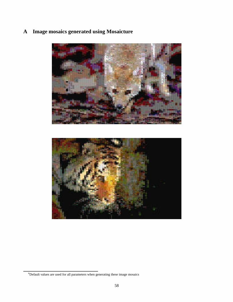
A Image mosaics generated using Mosaicture
4Default values are used for all parameters when generating these image mosaics
58

59

60

61

62
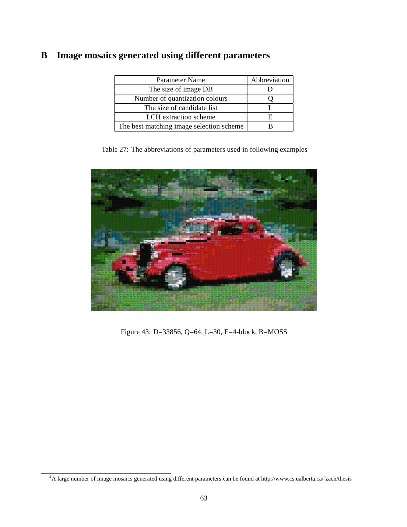
B Image mosaics generated using different parameters
Parameter Name AbbreviationThe size of image DB D
Number of quantization colours QThe size of candidate list LLCH extraction scheme E
The best matching image selection scheme B
Table 27: The abbreviations of parameters used in following examples
Figure 43: D=33856, Q=64, L=30, E=4-block, B=MOSS
4A large number of image mosaics generated using different parameters can be found at http://www.cs.ualberta.ca/˜zach/thesis
63

Figure 44: D=13846, Q=64, L=30, E=4-block, B=MOSS
Figure 45: D=33856, Q=8, L=30, E=4-block, B=MOSS
64
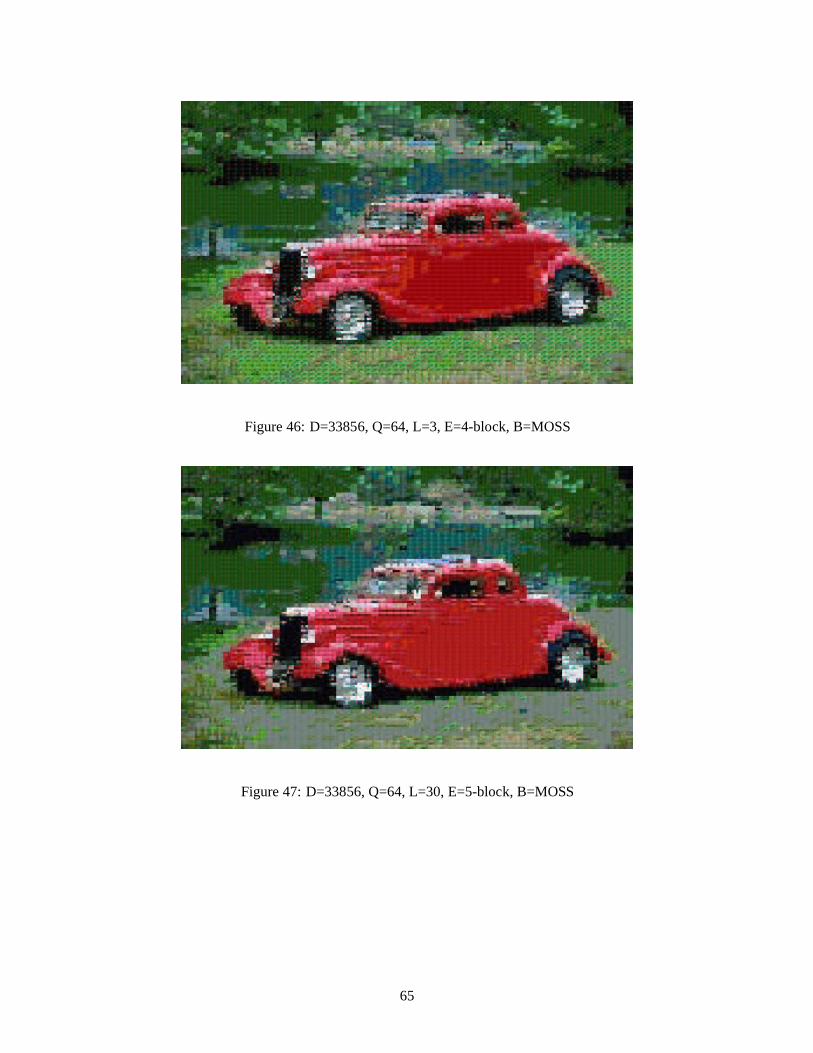
Figure 46: D=33856, Q=64, L=3, E=4-block, B=MOSS
Figure 47: D=33856, Q=64, L=30, E=5-block, B=MOSS
65
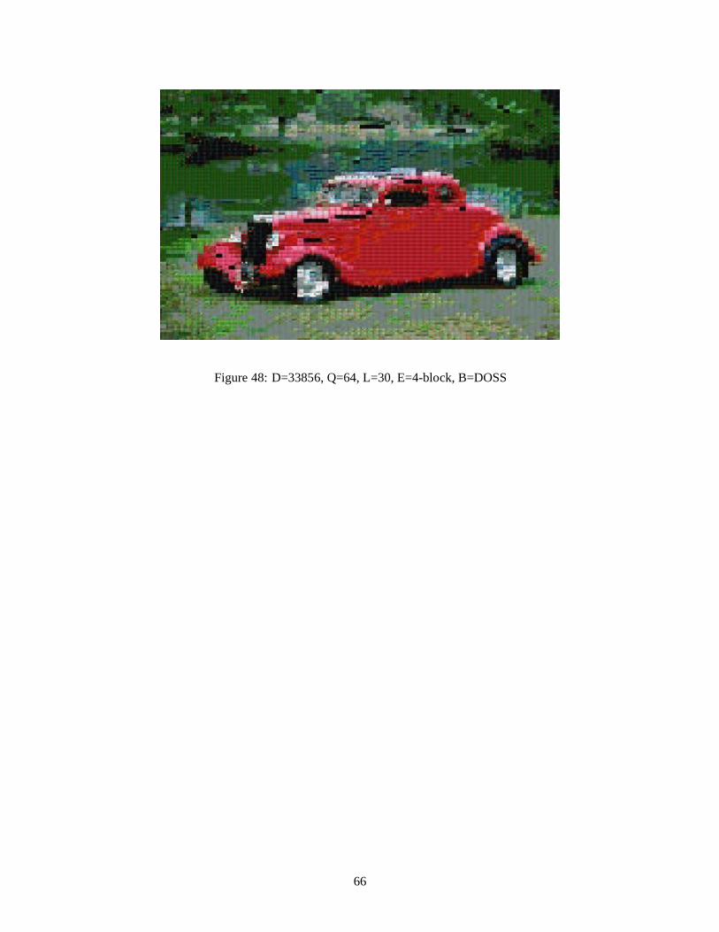
Figure 48: D=33856, Q=64, L=30, E=4-block, B=DOSS
66

C Detailed look at some example image mosaics
67
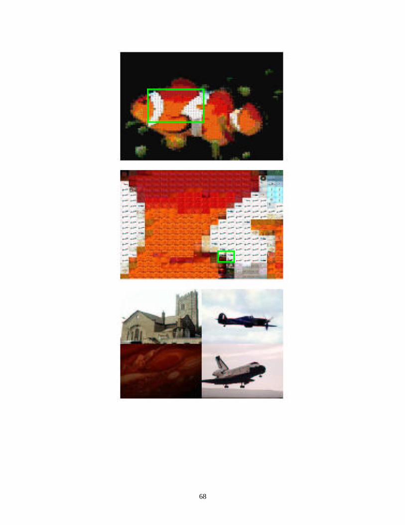
68

69
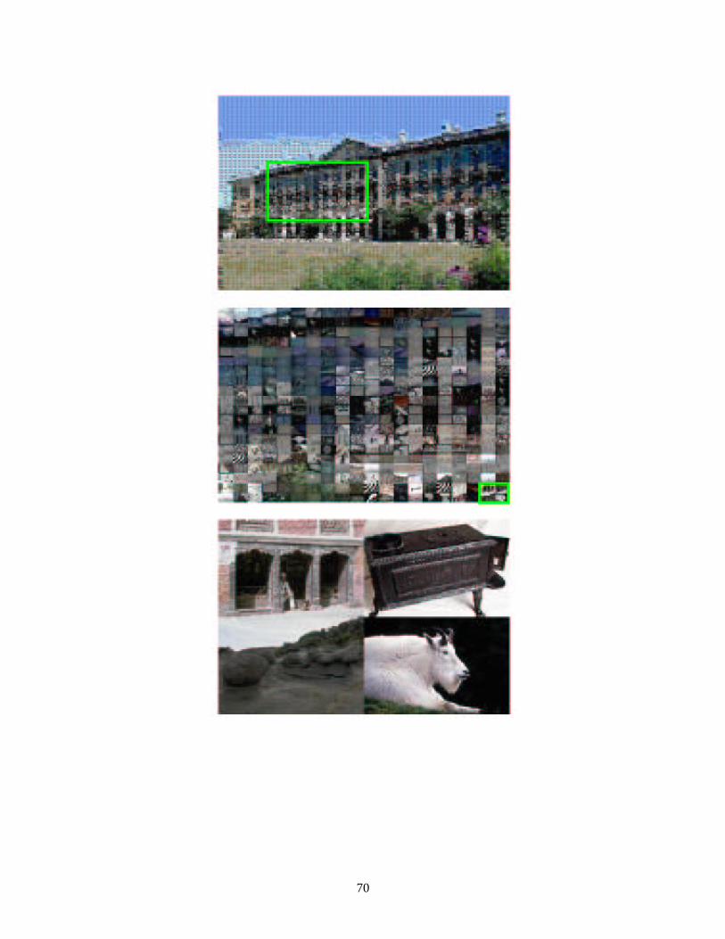
70

71