on the use of a frequency method for classifying the oscillatory behavior in nonlinear control...

On the Use of a FrequencyOn the Use of a FrequencyMethod for Classifying the Method for Classifying the

Oscillatory Behavior in Nonlinear Oscillatory Behavior in Nonlinear Control ProblemsControl Problems

Jorge L. MoiolaJorge L. Moiolain collaboration with G. Revel, D. Alonso, G. Itovich

and F. I. RobbioInstituto de Investigaciones en Ingeniería Eléctrica (IIIE)Instituto de Investigaciones en Ingeniería Eléctrica (IIIE)

Departamento de Ing. Eléctrica y de Computadoras, Departamento de Ing. Eléctrica y de Computadoras,

Universidad Nacional del Sur, Avda. Alem 1253, Universidad Nacional del Sur, Avda. Alem 1253,

(8000) Bahía Blanca, Argentina(8000) Bahía Blanca, Argentina

First Iberoamerican Meeting on Geometry, Mechanics and ControlFirst Iberoamerican Meeting on Geometry, Mechanics and Control

Santiago de Compostela, June 23 – 27, 2008

Outline

• Background and motivationBackground and motivation

• Harmonic balance approximationsHarmonic balance approximations

• Hopf bifurcationHopf bifurcation

• Double Hopf and fold-flip bifurcationsDouble Hopf and fold-flip bifurcations

• ConclusionsConclusions

Background

• Approximations play an important role in the analysis and control of nonlinear dynamical systems

• Several methods are available today• Dynamical systems theory (perturbation and

averaging) (Buonomo & Di Bello, 1996; Phillipson & Schuster, 2000)

• Not Discussed Today

• Control systems theory (frequency-domain approach) (Mees & Chua, 1979; Mees, 1981)

• Topic for today

Motivation: Frequency Domain Approach

• Detecting Hopf bifurcation (Moiola & Chen, 1993)

• Detecting multiple (degenerate) Hopf bifurcations(Moiola & Chen, 1994)

• Detecting the first period-doubling bifurcation (Rand, 1989; Belhaq & Houssni, 1995; Tesi, Abed, Genesio, Wang, 1996)

• Detecting cascade and global behaviors of oscillations (Belhaq, Houssni, Freire, Rodrígues-Luis, 2000; Bonani & Gilli, 1999)

• Reducing computational errors in Floquet multipliers (Choe & Guckenheimer, 1999; Guckenheimer & Meloon, 2000; Lust, 2001)

• …• Detecting nonlinear distortions

(Maggio, de Feo, Kennedy, 2004; Robbio, Moiola, Paolini & Chen, 2007)

Hopf Bifurcation

• An equilibrium point →→ a periodic solution

• If the bifurcation parameter is far away from the critical value, higher-order bifurcation formulas are needed.

A

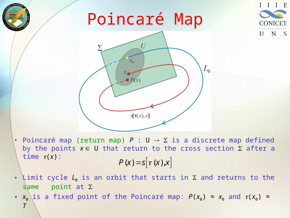
Poincaré Map

• Poincaré map (return map) P : U is a discrete map defined by the points x U that return to the cross section after a time (x):

• Limit cycle L0 is an orbit that starts in and returns to the same point at

• x0 is a fixed point of the Poincaré map: P(x0) = x0 and (x0) = T

( ) ( ),P x s x x

Stability Analysis (I)

• The stability of the periodic solution can be determined analyzing the state transition matrix Φ(t,0)

with

• Jvar (µ,t) is periodic with fundamental period

var( ,0) ( ) ( ,0), (0)t t t IJ

0

var( )

( ) ,x t L

ft

x

J

ˆ2 /T

The stability of the periodic solution L0 is determined

by the eigenvalues of the monodromy matrixmonodromy matrix M(µ)

( ) ( ,0)T M

where ( ; ),

n

p

x f x x R

R

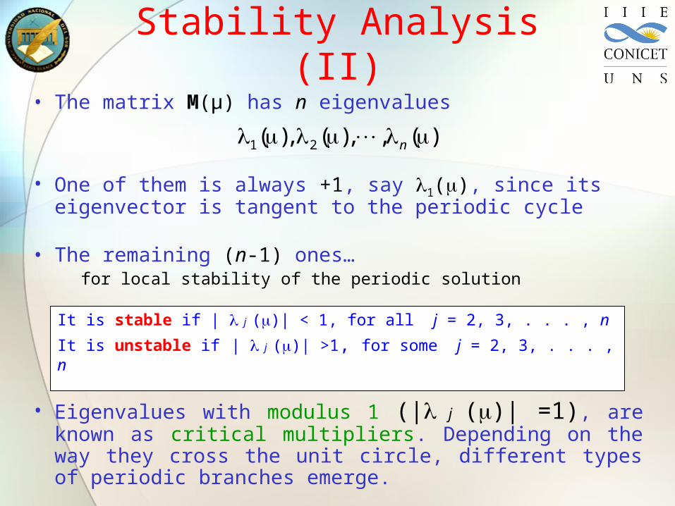
Stability Analysis (II)• The matrix M(µ) has n eigenvalues

• One of them is always +1, say 1(), since its eigenvector is tangent to the periodic cycle

• The remaining (n-1) ones…for local stability of the periodic solution

• Eigenvalues with modulus 1 (| j ()| =1), are known as critical multipliers. Depending on the way they cross the unit circle, different types of periodic branches emerge.

1 2( ), ( ), , ( )n

It is stable if | j ()| < 1, for all j = 2, 3, . . . , n

It is unstable if | j ()| >1, for some j = 2, 3, . . . , n

Types of Crossing

One eigenvalue at 1

One pair of complex-conjugate eigenvalues

One eigenvalue at +1

Types of Cyclic Bifurcations (I)

• One Eigenvalues at +1

• Fold bifurcation: saddle-node, pitchfork or transcritical

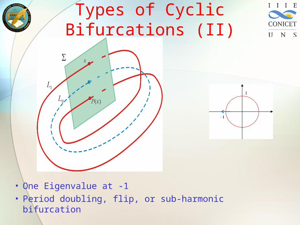
Types of Cyclic Bifurcations (II)

• One Eigenvalue at -1• Period doubling, flip, or sub-harmonic bifurcation

Types of Cyclic Bifurcations (III)

• A pair of complex-conjugated eigenvalues• Neimark - Sacker or Torus bifurcation

Time Domain Analysis vs Frequency Domain Analysis

• Stability analysis• Time domain: eigenvalues of Jacobian matrix• Frequency domain: eigenloci using Nyquist criterion

• Oscillation analysis• Time domain: time series• Frequency domain: frequency spectrum

• Bifurcation analysis ? --- Topic for today• Control system analysis? --- Not discussed

today

Frequency Domain Approach (I)

• Reformulate a general ODE system• There are many representations

• Following Mees & Chua (1979)• A linear system with transfer matrix

G(s;)

• A memoryless nonlinear feedback f(;)

( ; ),x x g y

y x

A B

C

[ ( ; ) ]x x y g y y

y x

A BD B D

C

1( ; ) [ ( ) ]s s G C I A BDC B

( ; ) : ( ; )u f e g y y D

with e y

Dimension may be reduced !

Frequency Domain Approach (II)

• Equilibrium points are solutions of

• The transfer function of the linearized system is G(s;)J(), with

• Eigenvalues are zeros of

• If one eigenvalue crosses over the imaginary axis, function h(,s;) has one root at = 1

(0; ) ( , ) 0f e e G

ˆ

( )e e

f

e

J

11 0( , ; ) det[ ] ( ; ) ( ; ) 0p p

ph s a s a s I GJ

Bifurcation Condition: from 0 =0 0( , ) ( 1, , )h i

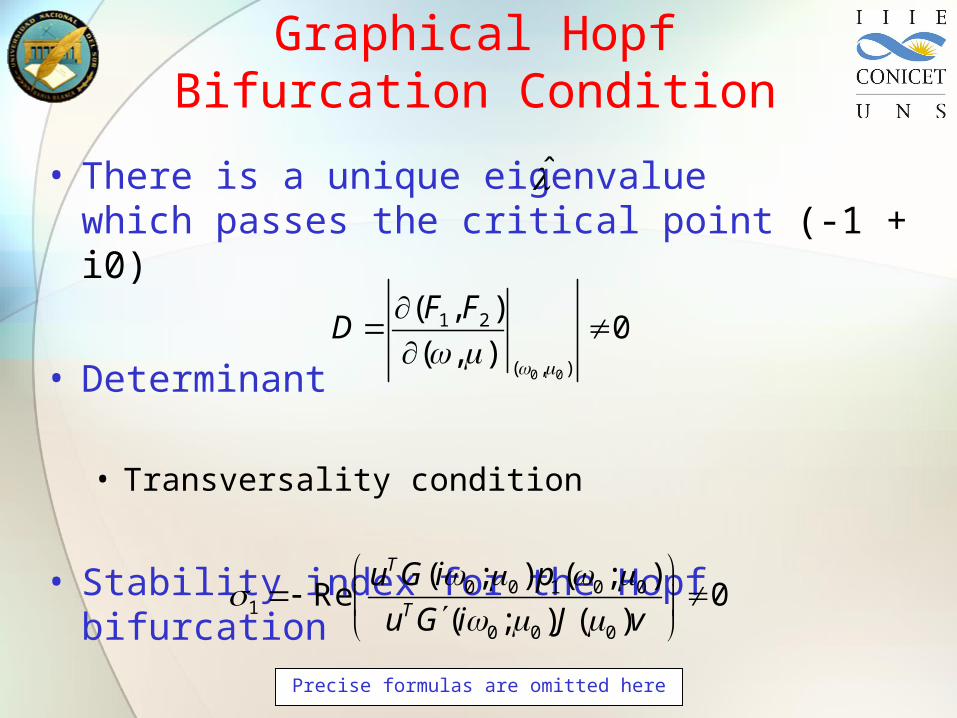
Graphical Hopf Bifurcation Condition

• There is a unique eigenvalue which passes the critical point (-1 + i0)

• Determinant

• Transversality condition

• Stability index for the Hopf bifurcation

0 0

1 2

( , )

( , )0

( , )

F FD

0 0 1 0 01

0 0 0

( ; ) ( ; )Re 0

( ; ) ( )

T

T

u G i p

u G i J v

Precise formulas are omitted here

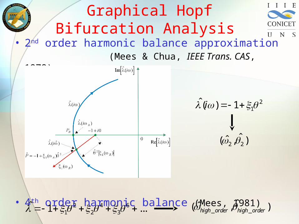
Graphical Hopf Bifurcation Analysis

• 2nd order harmonic balance approximation (Mees & Chua, IEEE Trans. CAS, 1979)

Eigenlocus

• 4th order harmonic balance (Mees, 1981)

21

ˆ( ) 1i

2 2ˆ( , )

2 4 61 2 3

ˆ 1 ... _ _ˆˆ( , )high order high order

Approximations of Periodic Solutions (I)

•2nd order 21( ) 1 ( )i

21( ) 1 ( )Ri

21( ) 1 ( )ii

( , )i i

1 1( , )

SOLUTION:

,R RP

Approximations of Periodic Solutions (II)

•From of 2nd order approximation

With

•q-order approximation of the periodic solution

with obtained iteratively from

1 120 1 22HB ˆ( ) Re j t j te t e E E e E e

1 1( , )

0 2 1 3 2 202 1 11 1 13 1 22 1, ,E V E V V E V

ˆ

HB0

ˆ( ) Re e ,q

qi ktk

qk

e t e E

21

1

ˆˆ ˆ( ) 1 ( )q

kq k q

k

i

( , )q q

In the step q :

N iterations

R RP

1( ) ( )Ri L i

1

2 1( ) ( )i L i

2

3 2( ) ( )i L i

3

4 3( ) ( )i L i

4

21 1( ) 1 ( )R RL i 2 42 1 1 1 2 1( ) 1 ( ) ( )L i 2 4 63 2 1 2 2 2 3 2( ) 1 ( ) ( ) ( )L i 2 4 6 84 3 1 3 2 3 3 3 4 4( ) 1 ( ) ( ) ( ) ( )L i

,ˆ ˆq q N

,ˆ ˆ

q q N

Computational Algorithm

Computation of the Monodromy Matrix (I)

• It is necessary to integrate• The original nonlinear system• The variational equation• This calculus is only possible

if we have an analytical expression of the periodic solution

• Approximate the monodromy matrix Mq

• The eigenvalues of Mq are the approximated values of the characteristic multipliers

var( )

( ) ( )q q

q

D Lx t L

ft t

x

J J

( ) ( ) ( )

(0)

2ˆ

qD

qq

t t t

Y J Y

Y I

M Y

Computation of the Monodromy Matrix (II)

• Since one multiplier must be +1, this property allows to determine the precision of the approximation

• The multiplier can be used for• If we are trying to find a cyclic bifurcation the

difference in the value +1, gives the error in the determination of the bifurcation.

• If we are approximating the cycle, the variation of this eigenvalue to the theoretical value +1, gives an indication of the validity of the approximation.

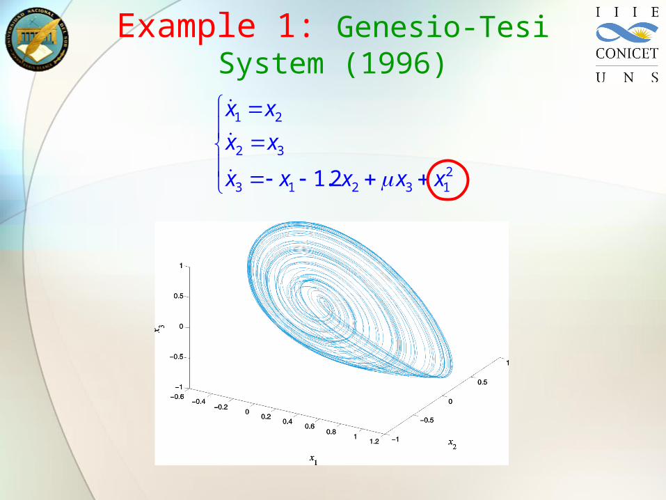
Example 1: Genesio-Tesi System (1996)

1 2

2 3

23 1 2 3 11.2

x x

x x

x x x x x

Example 1: Genesio-Tesi System (I)

0.46 0.6

1 2

2 3

23 1 2 3 11.2

x x

x x

x x x x x

Example 1: Genesio-Tesi System (II)

• SISO realization

• Hopf bifurcation

0 1 0 0

0 0 1 , 0 , 1 0 0 , 1

1 1.2 1

A B C D

21 1( )g x x

21 1 1( )f e e e ( ; )s G

1 1( ; ) ( ; ) 0f e e G 0

01 0,e

11 1,e NO

YES

ˆ( ) ( ) , with 1s s G J J

ˆ( ) 1 0j i 0

0

6 / 5

5 / 6R

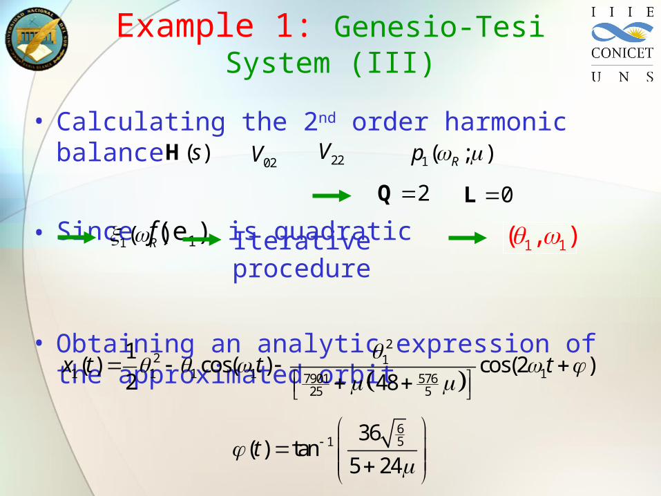
Example 1: Genesio-Tesi System (III)

• Calculating the 2nd order harmonic balance

• Since f(e1) is quadratic

• Obtaining an analytic expression of the approximated orbit

( )sH02V 22V 1( ; )Rp

2Q 0L

1( )R Iterative procedure

1 1( , )

2

2 11 1 1 1 17901 576

25 5

1( ) cos( ) cos(2 )

2 48x t t t

651 36

( ) tan5 24

t

Example 1: Genesio-Tesi System (IV)

•6th order harmonic balance approximation

1

0 1 0

( ) 0 0 1 ( )

1 2 ( ) 1.2

t t

x t

Y Y

PD 1 2 3

M3 -0.4885 1.00270 -1.00057 -0.05896

1maxPD 0.48096, , .0.7989 5 7803 . 30x T

1PD max 0.799360.4885, , .8827 5.7x T

% 1.57% 1max % 0.05%x % 0.09%T

M3

AUTO

Example 1: Genesio-Tesi System (V)

Double Hopf Bifurcation (I)

• Two pairs of complex conjugated eigenvalues of the linearized system cross the imaginary axis at two different frequencies

• Recent studies on voltage collapse in electrical power systems (Dobson et al., IEEE Trans. CAS, 2001)

• Nonlinear dynamics in high performance compressors for jets(Coller, Automatica, 2003)

Double Hopf Bifurcation (II)

• Recall: characteristic polynomial

• Using: generalized Nyquist stability criterion (MacFarlane & Postlethwaite, Int. Journal of Control, 1977)

• Obtained: Hopf bifurcation condition

( , ; ) det( ( ; ) ( )).h h s I G s J

1 0 0 0 0

2 0 0 0 0

( , ) Re ( 1, ; ) 0,

( , ) Im ( 1, ; ) 0.

F h i

F h i

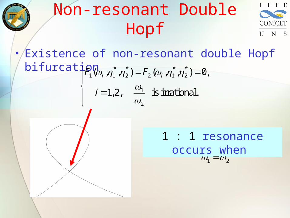
Non-resonant Double Hopf

• Existence of non-resonant double Hopf bifurcation * * * *

1 1 2 2 1 2

1

2

( , , ) ( , , ) 0,

1,2, is irrational.

i iF F

i

1 : 1 resonance occurs when

1 2

Resonant Double Hopf

• Existence of resonant double Hopf bifurcation * * * * * *

1 1 2 2 1 2

* * * * * *1 21 2 1 2

( , , ) ( , , ) 0,

( , , ) ( , , ) 0

F F

F F

Whitney umbrella

Using quasi-analytical approximations of limit cycles in the vicinity of Hopf bifurcation curves

Double Hopf Bifurcation: An Application

• Double LC resonant circuit (Yu, Nonlinear Dynamics, 2002)

Nonlinear element

311 1 1 1 2 1 4 1 12

22 12

3 4

4 1 3 2 4

,

,

( 2 1) ,

(2 2)( ),

x x x x x

x x

x x

x x x n x

312G G Gi v v

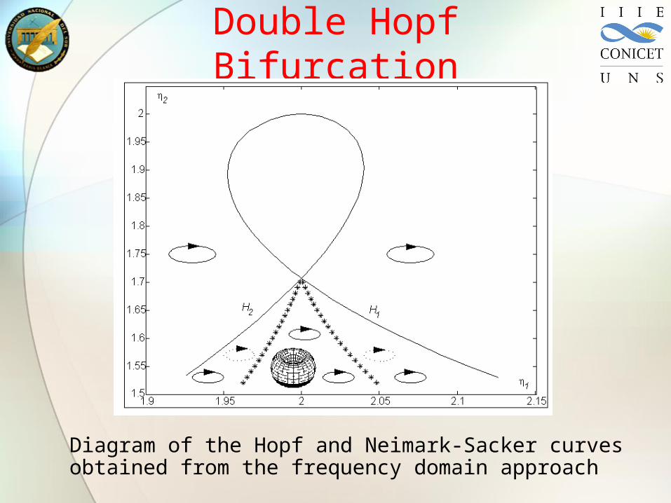
Double Hopf Bifurcation

Diagram of the Hopf and Neimark-Sacker curves obtained from the frequency domain approach

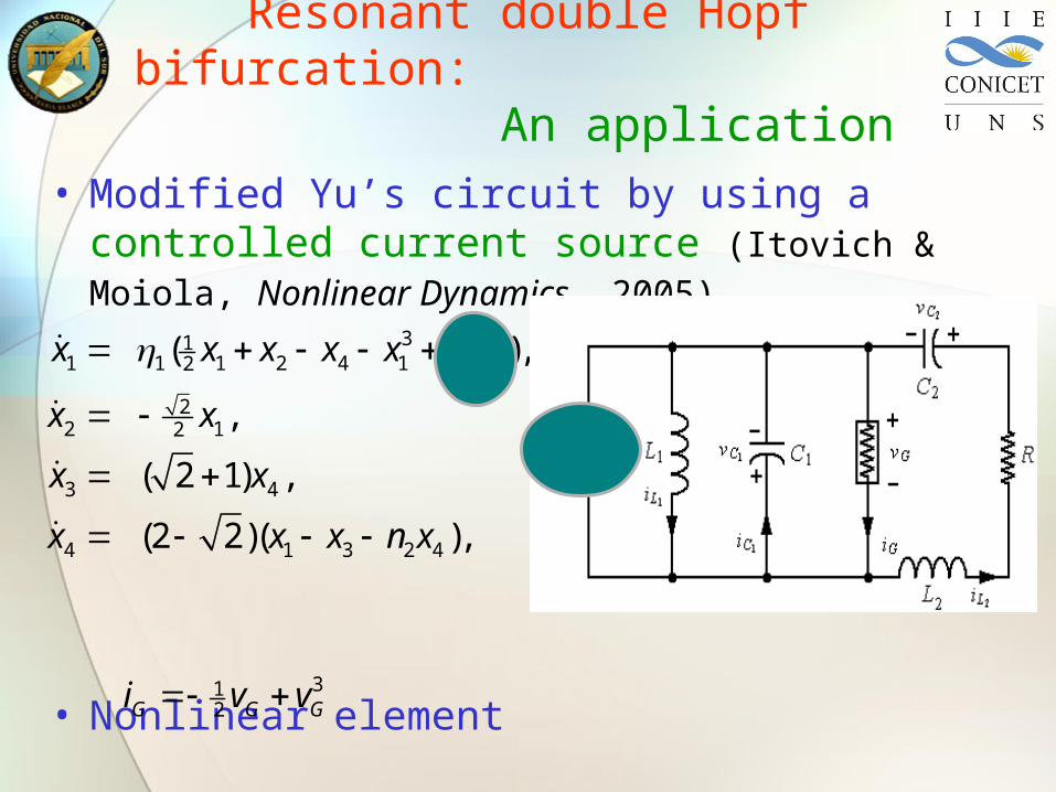
Resonant double Hopf bifurcation: An

application• Modified Yu’s circuit by using a controlled

current source (Itovich & Moiola, Nonlinear

Dynamics, 2005)

• Nonlinear element

3

1

311 1 1 2 4 1 22

22 12

3 4

4 1 3 2 4

( ),

,

( 2 1) ,

(2 2)( ),

x x x x x x

x x

x x

x x x n x

312G G Gi v v

Whitney umbrella for the controlled system

Hopf bifurcation curves of the modified Yu’s circuit

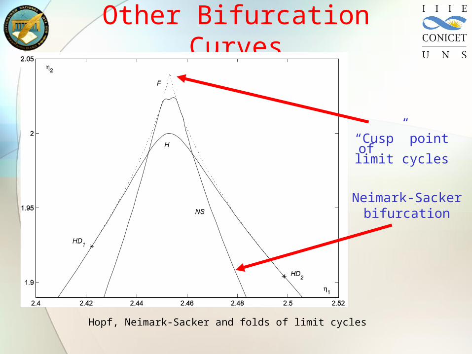
Other Bifurcation Curves

“Cusp” point of limit

cycles

Neimark-Sacker bifurcation

Hopf, Neimark-Sacker and folds of limit cycles

Neimark-Sacker curves in the modified Yu’s circuit

* LOCBIF — frequency domain method

Fold curves in the modified Yu’s circuit

* LOCBIF — frequency domain method

Continuation of Limit Cycles (I)

* LOCBIF — frequency domain method o XPP-AUTO

Continuation of Limit Cycles (II)

* LOCBIF — frequency domain method o XPP-AUTO

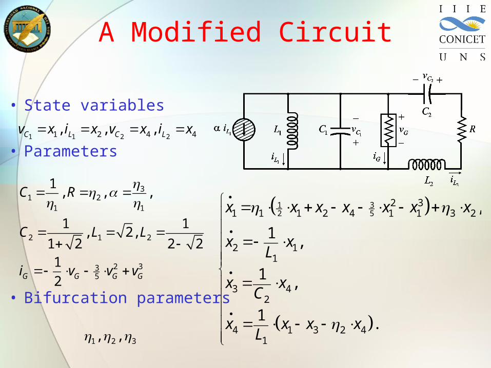
• State variables

• Parameters

• Bifurcation parameters

31 2

1 1

2 1 2

2 335

1, , ,

1 1, 2,

1 2 2 21

2G G G G

C R

C L L

i v v v

312 5

2 31 1 1 2 4 1 1 3 2

2 11

3 42

4 1 3 2 41

,

1 ,

1 ,

1 .

x x x x x x x

x xL

x xC

x x x xL

1 1 2 21 2 4 4, , , C L C Lv x i x v x i x

1 2 3, ,

A Modified Circuit

Model Features

• The origin is the only equilibrium point• Two pair of complex eigenvalues on the

imaginary axis

with frequencies

• Both frequencies are equal for

1 3 2 3

2 12 , 1 1 ,

2 2

2 21 11,2 3 32 42 , 3 (1 2) .

41 2 3 1,28 4 2, 2, 6 4 2, 2.

Bifurcation Analysis

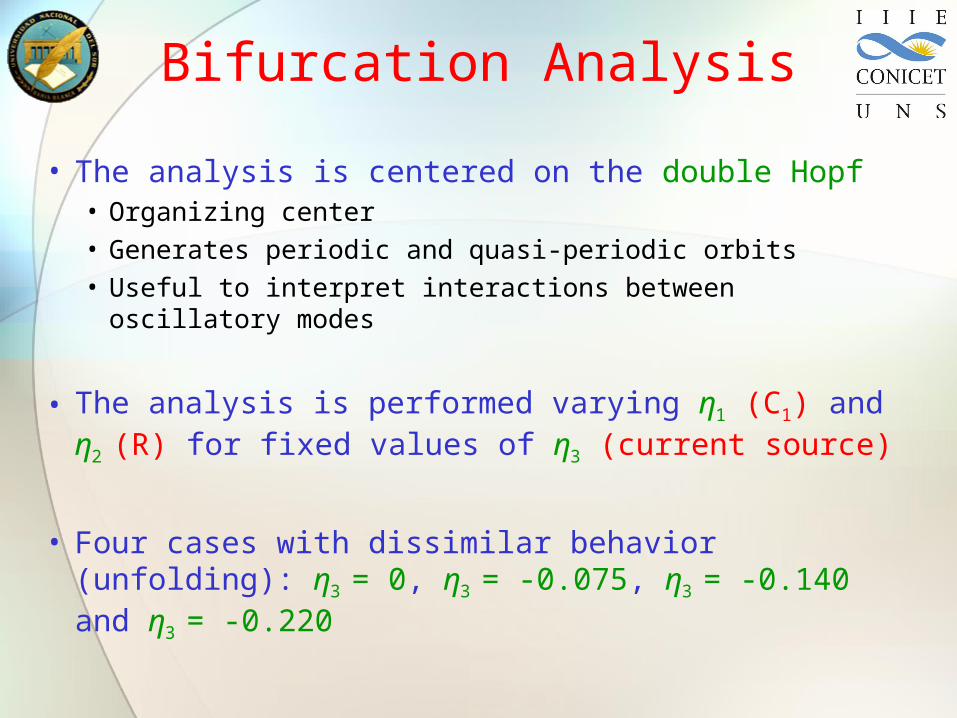
• The analysis is centered on the double Hopf• Organizing center• Generates periodic and quasi-periodic orbits• Useful to interpret interactions between oscillatory

modes

• The analysis is performed varying η1 (C1) and η2 (R) for fixed values of η3 (current source)

• Four cases with dissimilar behavior (unfolding): η3 = 0, η3 = -0.075, η3 = -0.140 and η3 = -0.220

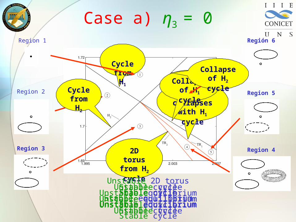
Case a) η3 = 0Region 1

Cycle from

H1

Region 2

Stable equilibriumUnstable equilibrium

Stable cycle

Cycle from

H2

Region 3

Unstable cycleUnstable equilibrium

Stable cycle

2D torus from H2 cycle

Region 4

Unstable 2D torusStable cycle

Unstable equilibriumStable cycle

2D torus collapses

with H1 cycle

Region 5

Stable cycleUnstable equilibrium

Unstable cycle

Collapse of H1

cycle

Región 6


Collapse of H2 cycle

Case b) η3 = -0.075Region 1

Region 2

Region 3

Region 5

Region 6

Same as before

2D torus from H1

cycle

Region 7

Stable 2D torusUnstable cycle

Unstable equilibriumUnstable cycle

2D torus collapses

with H2 cycle

Case c) η3 = -0.140

Same as before

Region 1

Region 2

Region 3

Region 6

Region 7


Region 8


Unstable equilibrium

2D torus collapses

with H2 cycle

Case d) η3 = -0.220Region 9

Unstable equilibrium

Cycle from

H2

Región 10


Cycle from

H1

Región 11


Unstable cycle

2D torus from H1 cycle

Region 12

Unstable 2D torusUnstable cycle


Region 13Stable 3D tours & Unstable 2D

torusUnstable cycle


Region 14



2D torus collapses

with H2 cycle

Region 15


Region 16


Unstable cycle

Stable equilibriumUnstable cycle


Simulations: Case d) regions 12, 13 & 14 (η2 = 1.88)

• Region 12: Unstable 2D torus

• Region 13: Stable 3D torus

• Region 14: Stable 2D torus

1 20.1285 Hz, 0.2130 Hz.f f

1 2

3

0.1285 Hz, 0.2130 Hz,

0.0001 Hz.

f f

f

1 20.1285 Hz, 0.2130 Hz.f f

Simulations: Case d) region 15 (η2 = 1.88)

• Region 15: Stable limit Cycle

2 0.2174 Hz.f

Fold-flip Bifurcation

• Also, there are two fold-flip bifurcations for η3 = -0.140

• Both are located over a tiny period doubling (or flip) bifurcation “bubble” close to the double Hopf point

• This is a co-dimension 2 bifurcation of periodic orbits• Floquet multipliers at +1 (fold) and -1 (filp)• Tangent intersection between a cyclic fold

and a flip curve• Rare in continuous systems

• Studied via numerical continuation

Cyclic Fold Bifurcation

Flip Bifurcation

Schematic Representation

• Two different unfoldings

• Continuations above and below the FF points

• Global phenomena make possible the coexistence of both FF points

3 0.140

Double HopfFlip “bubble”

Cyclic Fold

Above FF1: η2 = 1.755

a a’

Below FF1: η2 = 1.747

b b’

Region 1• Stable cycle• Unstable cycle• Unstable PD cycle

Normal Form of FF1

Region 2• Stable cycle• Unstable cycle

Region 3• No cycles

Region 4• Unstable cycle• Unstable cycle

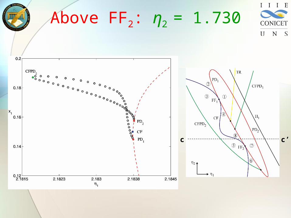
Above FF2: η2 = 1.730

c c’

Below FF2: η2 = 1.728

d d’

Normal Form of FF2

Region 5• Unstable PD

cycle

Region 6• Unstable cycle• Unstable cycle• Unstable PD cycle

Region 7• Unstable cycle• Unstable cycle

Region 8• Unstable PD cycle• Unstable cycle• Unstable cycle

Applications in Power Systems

Conclusions

• Frequency domain approach to bifurcation analysis• Reducing dimension, so reducing the complexity of

analysis• Graphical and numerical, therefore bypassing some

very sophisticated mathematical analysis• Applicable to almost all kinds of bifurcation analysis• Relatively heavy computations are generally needed• May be combined with LOCBIF and XPP-AUTO

• Other applications• Nonlinear signal distortion analysis in electric

oscillators• Bifurcation and chaos control

Thank you!

• E-mail: [email protected]

on the use of a frequency method for classifying the oscillatory behavior in nonlinear control...

Documents