on the statistical solutions of the two-dimensional, periodic euler equation
TRANSCRIPT

Math. Meth. in the Appl. Sci. 7 (1985) 55-73 @ 1985 B. G. Teubner Stuttgart
On the Statistical Solutions of the Two-Dimensional, Periodic Euler Equation
S . Caprho*) and S . De Gregorio, Roma
Communicated by H. Neunzert
We investigate the problem to define statistical solutions for the two-dimensional. periodic Euler Equation and prove a theorem of global existence and uniqueness for a regularized version. Moreover, we deduce the existence of the Euler flow in a weak form.
0 Introduction
Let us consider the Euler equation for an incompressible, non viscous fluid in the two-dimensional torus T 2 = [ - x , n ] x [ -n ,n] , in terms of the vorticity o :
am (0.1) - + ( U ’ 0 ) O = 0
a t
au, au, . ax, ax,
w = curlu = - -
divu = 0
w(-x ,x2 , t ) = w ( n , x , , t ) ; w ( x , , - x , t ) = o ( x , , n , t )
where x = (x, ,x2) is a vector in T2, u = (u, , u2) is the (solenoidal) velocity field and o is a scalar. Since divu = 0 there exists a “stream” function ‘Y. such that
ay/ a y u = 0; Y = (- ax,, K). This implies that an equivalent version of equa- tions (0.1) is
aw (0.2) - + (U‘ V)o = 0
a t
*) Work partially supported by the Italian C.N.R.

56 S. Caprino and S. De Gregorio
with the same boundary conditions, where gp is the fundamental solution to the Poisson equation in T 2 :
A s p = 8,
8, being the periodic &function. As it is well known, the Euler evolution for w is given in terms of the
evolution of the fluid particles, which move following the characteristics induced by the velocity field u.
Existence and uniqueness of classical solutions of (0.1) are known since a long time (see for example [l]). Existence and uniqueness of weak solutions is proven in 121 (see also [3], where the result is proven for a very large class of initial data, that is L’ n L”).
Another class of solutions for which it is worthy to find existence results consists of the so called “statistical solutions”. In fact the individual solutions, i.e. the evolution of the a ’ s , may give a detailed and too complicated picture of the fluid, while one could be interested in the behaviour of some global quantity related to the fluid. This is as in Statistical Mechanics, where “microscopic” picture is replaced by a “macroscopic” one, by means of averages with respect to some relevant probability measures. Obviously, we can define this macroscopic evolution in terms of the evolution of the a ’s , but there is the problem to choose a physically significant set of a ’s , good enough to give all relevant features of the fluid. The hypothesis of the Statistical Mechanics is that such a set must have measure one with respect to the “Gibbs measure”, which is invariant for the flow. (General discussions on the importance of the statistical solutions to the Navier Stokes and Euler equations can be found in *) and **).) The construction of such invariant measures looks quite natural, since the Euler equation has the nice property to admit infinitely many first integrals, as the energy E = 5 u’dx, the enstrophy S = 5 w2dx and I, = 5 f(w (x) )dx for any continuousf.
T2
72 T2 In 141, [5], 161, the authors construct measures which are formalb
invariant along the 2x-periodic solutions of the Euler equation; they also pose the problem whether these measures are really invariant, or equicalently whether the Euler flow can be defined. Unfortunately, the Gibbs Measures that we can define by means of the energy and enstrophy, are supported on w’s which make these constants of motion possibly infinite. This implies that neither these first integrals are available to get an a priori estimate, nor the field u is in general defined. We stress that all known results on existence and uniqueness, are for sets of initial data of measure zero, not relevant for statistical purposes (see the discussion on this point in Section 1).
In this paper, we consider a weak form of the 2x-periodic Euler equation for a’s that are in the support of the measure ,us, related to the enstrophy. Un- fortunately, in this case the Euler equation is, in general, not even well posed.
*) Chorin, A. J.: Lectures on Turbulence Theory. Mathematical Lecture Series 5. **) Glaz, H. M.: Lecture Notes in Mathematics, 615, Turbulence Seminar, p. 135.

On the Statistical Solutions of the Two-Dimensional, Periodic Euler Equation 57
Hence, we introduce a modified Euler equation, by suitably cutting off the singularity of g,. This implies that the velocity field is well oefined, at least at time zero. In Section 3 we give a result on existence and uniqueness of statistical solutions of this problem.
We were motivated to introduce this somehow artificial model by the following considerations. We are still concerned with a system with infinitely many degrees of freedom, since no Fourier component of w is eliminated. More- over, the enstrophy is untouched and the invariant measure does not depend on the cut-off. The plausibility of our assumption on gD is supported by two facts:
N
i = I (a) if the initial condition is given by o = C 6,. being the &function centered
at the point x , , then we have the vortex model, for which it has been proven in [7] that the evolution given by the regularized g, coincides with the true evolution, with probability one with respect to the normalized Lebesgue measure in T 2 N ; (b) consider the two-dimensional Vlasov equation. It has the same features as the EuIer equation, save that the equation of motion for the (fluid) particles is a dynamic (not kinematic) differential equation. Therefore, in this case, the assumption that the particles interact via a regular potential, is reasonable from a physical point of view.
Then our result includes case (a) and may be a first step to the solution of problem (b). (For a discussion on individual and statistical solutions of the Vlasov equation, see [8] and [9] respectively.)
In section 4, we show that the cut-off can be removed, so that the solution of the regularized problem converges in L2(Q,pu,), SZ being the space of a’s, to a solution of a very weak Euler equation (see Theorem 4.3 for the exact statement of the result). Unfortunately, since we use compactness arguments, we cannot exhibit any uniqueness property.
Our result gives the time evolution of any meausre v , such that
v ( d o ) = f (w)Ps(do)
v , (A) = V(T-,A)
for somefe L2(SZ,ps), defining
for any psmeasurable set A, T, being the Euler flow on SZ.
1 Preliminary considerations
Let us write equations (0.2) in Fourier components. For the moment, we do not make any smoothness hypothesis on w , and all integrals and series which appear in this Section are only formally written.
Since.any function on T 2 can be thought as a 2x-periodic function on R2, we associate to w its Fourier series:

5 8 S. Caprino and S. De Gregorio
with
By (0.2), u is a periodic vector field, given by
on the boundary of TZ, and this implies the condition
0 0 = j w ( x ) d x = 0 T2
by the circulation theorem. Then, system (0.2) takes the form:
Furthermore, we have to impose the reality condition:
(1.2) 0, = & - k .
It is easily seen, and it is indeed well known from the classical theory of incompressible, non viscous fluids, that system (1 .l) admits the following first integrals :
c Iw,I2:= S(w) 1 Enstrophy = -
(2n)2 kat2
lwkI2 c -:= E ( o ) . 1 Energy = - ksf2 k2
If w is smooth enough, then T,, S and E are well defined functions of w . We want now to stress some interesting facts, which will lead us to a
Let C be the complex plane and let p' be the probability measure on C choice of the 0's in an unusual and wider class.
defined by
with O , E C . Then a probability space can be constructed in a standard way as
(QdJ = n ( C , P k ) k€Z2

On the Statistical Solutions of the Two-Dimensional, Periodic Euler Equation 59
where an element w of s2 is a sequence {Wk}k&, wk E C and ps is a probability measure defined on the a-algebra generated by the cylinders in Q.
Remark 1.1 Note that C a yk(w) = 0, since every term in the formal series
is zero, with Vk(w) given by (l.l), so that the vector field in s2 V ( o ) = { ~(w)}k,zzis formally solenoidal. This, together with the enstrophy conserva- tion implies that the measure,us is formaiiy invariant along the solutiorls of (1 .I).
We are now interested in finding a support for the measure ps. To this purpose, let us consider the subset of s2:
8, = {w E n : 3a(w) E R + : )wkl< (r(0) I/hl(k( Vk€ z2 , (kl > 1 .
k c t z
-___
Proposition 1.1 ps(Qo) = 1.
P r o o f .
Q; = R/Q, G n u .%k,a aeO+ k e f z a > l lkl> 1
where Q + --_- is the set of positive, rational numbers and
We have:
= {w E Q : I o k I 2 aVInIkI}.
p,(s2Q < lim C P,(.?dk,=) = lim C - 1 s _ e - lwklzdwk a d m ketz a+- kefz X J w k l > a l h lk(
PI> 1 lkl> 1
and the theorem is proven. For any o E s2, and f E Vm ( T 2 , R), set:
withf, the k-th Fourier coefficient off.
Define moreover:
Let us consider the set:
(1.5) 9= ( ~ E R : ~ c ( o ) > O:(w(f)I< c(~)Ilfll2,~, v ~ E ~ ~ ( T ~ , R ) } .
V r n ( T 2 , R), continuous in the norm ( 1 f 112,,, . Then g2 is a linear space of distributions, i.e. linear functionals on

60 S. Caprino and S. De Gregorio
The following holds:
Proposition 1.2 52, C P2.
P r o o f . Let o E 52,. By the Schwartz inequality and the Parseval theorem it is: 1 I 2
ksZ
withd(o) = - ( 5 ,,,)‘I2 c m. This implies: . (2X)Z ke 2 k4
Io(f>I < a(wlIIfII2,m
having chosen a(o) = ( 2 n ) d ( ~ ) .
Propositions 1.1, 1.2 show that 52, (and then p2) is a support for the measure ,us. Then, if we were able to construct the Euler evolution for any o in one of these sets, then ps would be an invariant measure for this flow. Unfortu- nately, the right hand side of (1 .l) may be not well defined for any choice of w in SZ, and in fact initial conditions for which Pk is absolutely convergent (and then no ambiguity arises in the sum) are in a subset of Q,, of measure zero with respect tops.
In the next Section, we will introduce a modified Euler equation, good enough to represent a time-evolution of o ’ s in 22.
2 Regularized Euler equations
The regularized version of the Euler equation that we are going to define, is obtained by cutting off the singularity in the periodic Green function g,(x), as if a continuous spherical distribution of “charge” was smeared around the origin. Obviously, this model reduces to the original one, as the cut-off is removed.
To be more precise, letf‘ E ‘6‘” ( T2, R +) be a one-real parameter family of functions, as E ranges over some positive interval ]O,C[, having the following properties:
(a) f”(x) = 0 iflxl> - 2
(b) fe(x) = F ( x ’ ) iflxl = Jx’lmod2n
(c)
&
5 f ” ( X ) d x = 1 . TZ
Then, the corresponding Fourier coefficients fk(&) must satisfy, for any x k E Z2 and E E 10, E [ , E > -:
(d)
4
fk(&) is real and 1 fk(&) I < 1

On the Statistical Solutions of the Two-Dimensional, Periodic Euler Equation 61
Consider the function:
@ & ( x ) = j f‘(x - Y ) f ‘ ( Y ) d Y . (2.1)
It is easily seen that @ & E ‘ P ( T 2 , R + ) and satisfies the following:
Properties 2.1 (i) @ ‘ ( x ) = 0 if Ix I> E and @‘(x) > 0 otherwise.
(ii) @‘(x) = @‘(x’) if 1x1 = Ix’Imod2n (iii) j @‘(x)dX = 1 V E E ] O , ~ [
which implies
TZ
T2
1 (2.2) @ ‘ ( x ) < const. - V E E ] O , E [ a n d x e T 2 . E 2
Furthermore, for the Fourier coefficients we have:
This function has the following properties: (A) is a 2x-periodic, smooth function with Fourier coefficients
(B) g ; ( X ) = 9Jx) i f lxl> E .
(C) Call v‘(dx) = @‘(x)dx. Then, Properties 2.1 (i) - (iii) imply:
weak limv‘(dX) = aPdx ‘-0
which in turn implies
lim $ ( x ) = gp(x) . & d O
Remark 2.1 Property (B) is simply the Gauss Theorem: a point charge and a charge symmetrically distributed in a sphere of radius E , produce the same effect

62 S. Caprino and S. Dc Gregorio
outside the sphere. Moreover, property (C) gives the relation between the modified and the actual Euler equation: the latter is obtained as singular limit of the former.
We state now the regularized version of the Euler equation (1 , l) , (1.2).
and the series defining Y i(w) is absolutely convergent, by property 2.1 (vi). System (2.5) admits the following invariants:
1 (a) S(O) = - 1 lwk12
(2X)2 keZZ
that is the usual enstrophy. If w E Q2, by Proposition 1 .l, it can be easily seen that S(o) is p, - almost everywhere unbounded and then only formally invariant.
In fact:
2 h L - k c - w k o h w h ' @ h ( & ) @ k ( & ) (2.5) (2X)2 h,h'.keZ2 h2k2
h + h ' + k - O
and the coefficient of w k w h o . ) h ' , obtained by the sum over all permutations of the three indices, is zero, by the properties of @ and of the operator (.)I.
By (2.6), EE(cu) is finite and positive for any w E 92. We will look for the solutions of (2.5) in %*. System (2.5) is equivalent to
the weak form of the regularized Euler equation:
0 0 = w
Let v be any time-dependent vector field in T 2 and consider the one-para- such that coo = w and for any t 2 0 and
for any f E ' P ( T 2 , R), with of = { a k ( t ) ) k & .
meter family of distributions f E Va(T2, R) satisfies
(2.8) w,cn = o(fr")

On the Statistical Solutions of the Two-Dimensional, Periodic Euler Equation 63
where f y , the “translated” off, is defined by
f ;cx> = f (x(t, x ) ) x( t , x ) being the solution to the Cauchy problem
(2.9) X = v(x, t ) ~ ( 0 ) = X .
Then, w t satisfies the identity:
In particular, if v = u‘, such family w t satisfies the (non linear) Euler equation. In [3], it has been proven that the (unique) solution to the Euler equa- tion, with initial condition w E L”, satisfies property (2.8), with v replaced by u defined in (0.2). Thus, also in our case, we will look for solutions to (2.5) of this kind. We stress that in the classical case, (2.8) is authomatically satisfied by the solution, since the Euler equation is a conservation law for the vorticity, along the stream lines induced by u.
In order to find the solution at to (2.5). we have to prove the existence of the solution to (2.9) with respect to the solenoidal vector field uc(x, t ) . This means that a, would be known, once the motion of the fluid particles x ( t , x ) is known, as solutions of (2.9). On the other side, ue depends on 0, itself: this implies that we cannot know at a glance whether (2.9) admits or not a solution.
We now state our main result, which will be proven in the following Sec- tion. Theorem 2.1 For any E E ] O , E [ , there exists a unique one parameter group of mappings
Tf: 9 2 + 9 2 9 0 -+ TfU = {wi(t)}kez2
such that o”;.t) satisfies the Cauchy problem (2.5) for any t E R and 0, satisfies ( 2 . Q with v = ue.
Corollary 2.1 The rneasurep, is invariant along the f low induced on g2 by Tf .
3 Proof of Theorem 2.1
Step I : Some preliminary estimates for a linearized version of problem (2.5). For any w E g2, set
This quantity is finite by (2.6) and Property 2.1 (vi). Moreover, ) I w
Given w E g2, let ({ = f(J (t)}ksZ2r t E [O,T] T arbitrary and positive, < PO.
‘ k j = 1,2, be two one-parameter families of distributions in Q2, such that
(3.2) (((0) = wk vkeZ2

64 S. Caprino and S. De Gregorio,
and _-
(3.3) Ilr’kll< B L m W )
v t E [O,T], j? > 1 not depending on t. (For the sake of simplicity in the notations, we will not keep the superscript E on u . )
Let us consider the following linearized version of problem (2.5)
O&(O) = O-&(O) = W & .
The solution 0: = { ~ j k ( f ) } ~ ~ p to (3.4) does exist in [O,T], given by
(3.5) 4(f) = w;) for any f E W”(Tz, R), where f$ is the translated off by the vector field:
In fact, by the good properties of t.(, U J is a smooth vector field and the solution to the Cauchy problem
(3.7) A? = U’(X , t ) x(0) = x
does exist unique in [O,T]. Thus, also w{ exists, unique in the class of distribu- tions satisfying (2.8).
Our goal in this first step is to estimate the quantity O! - O: in terms of the difference <f - t,”, After straightforward calculation, we obtain:
(3.8) loi(t) - o:(t)I = Io.(e- i k . X 2 ( l . X ) - e-ik.x’(l,X))I i k . X 2 ( f , X ) - e-ik.x’(r.x) < c(o)lle- 112,-
< C(~)lkI311X2(t ,X) - x1(Lx)I12,0. ~ ~ l l ~ 2 ~ ~ A l l ~ , ~ ~ z + ( t I ~ ~ ( t ~ ~ ) t I ~ , r n ) ’ I
where, if y = (y, (x), y2(x)) is a vector function, we have put:
and 11 - ll;.,,, is the same as )I - 1 1 2 , m , but the sum is taken over i, + i2 = i > 0. To
simplify notations, in what follows I 0, f I will stand for [(%r + ( ~ y ] ” ~ , = 1,2, i f y is a vector function function, and] V,yl for
and analogously for I V i f I and I V i y 1, 1, s = 1,2.
On the Statistical Solutions of the Two-Dimensional, Periodic Euler Equation 65
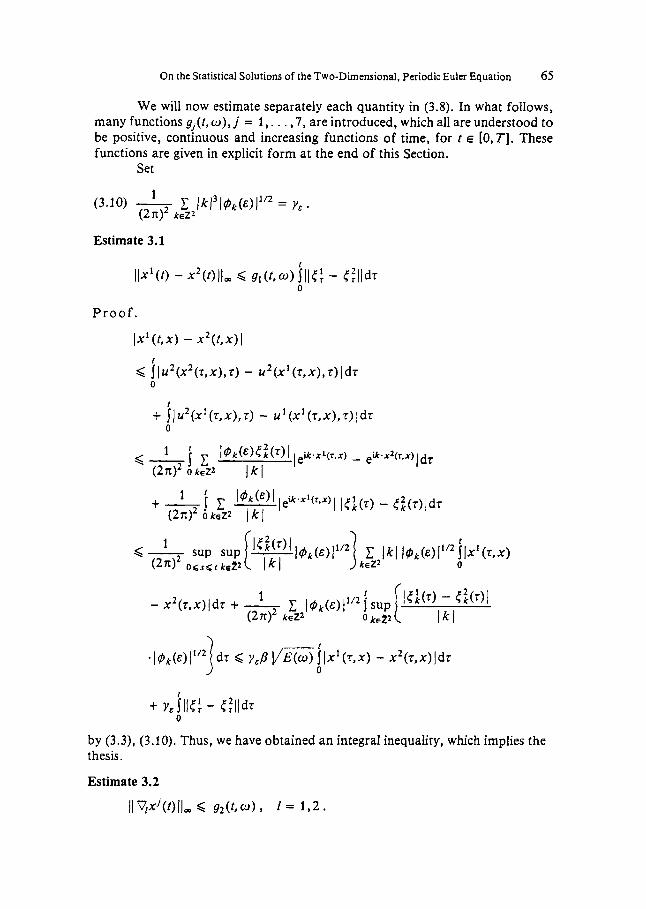
We will now estimate separately each quantity in (3.8). In what follows, many functions g,(t, a), j' = 1,. . . , 7 , are introduced, which all are understood to be positive, continuous and increasing functions of time, for t E 10, T]. These functions are given in explicit form at the end of this Section.
Set
' 0
+ j 1 u2 (x' (5, x), r ) - u (x' (5, x), T) 1 dr
< 5 I u 2(xZ(?, x), r ) - U 2 (XI (5, x), r ) I dT
t
0
t
0 + YeSllt: - tflP
by (3.3), (3.10). Thus, we have obtained an integral inequality, which implies the thesis.
Estimate 3.2
llqxqt)llw < 92(t ,o) 9 1 = 192 *

66 S. Caprino and S. De Gregorio
P r o o f .
* 1 ti(') - I I Fx l ( T J x ) 1 dT '
The thesis follows from analogous arguments as those used in Estimate 3.1, via all previous results. Estimate 3.4
IIVZ,xi(t)II, < g&JO) , Ls,j = 1 , ~ .
I V i x ' ( t , x ) I
P r o o f . By easy computation:

On the Statistical Solutions of the Two-Dimensional, Periodic Euler Equation 67
and the thesis is easily achieved, by all previous Estimates.
the following:
Proposition 3.1
Let us now go back to (3.8). All the above results enable us to establish
llof - dl< g,(t, 0) ill<: - 5f l ldr . 0
Proof . By Estimates 3.1 -3.5, we can conclude that there exists g6(t,o) such that:
I
0 lo:(t) - o:(t)l< L?6(t,a)Ik13111<: - t:lldr.
Thus, by Definition (3.1) and (3.10), the thesis immediately follows.
Given o E 9z, let us define the following sequence: Step 2: An iterative algorithm.
0: = (o;(t):,,Zz
6 0 = 1 - 0
I E [O, 7-1 , T arbitrarily large and positive, such that:
I , u k ( t ) l k e Z z = o for any t~ [O, T I
for any n E Z+/(O), t E [O,T], o;(t) being the solution of the linear Cauchy problem:
S. Caprino and S. De Gregorio 68
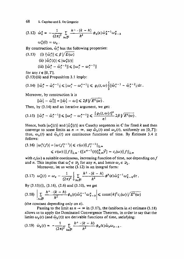
(3.12)
By construction, 6: has the following properties: (3.13) (9 rrqrr 2 B 1/Elw)
(ii) I+:(t>l < lo;(Ol (iii) I!+: -
for any t E [O, TI. (3.13) (iii) and Proposition 3.1 imply:
(3.14) 116: - &:-'I/ < 110: - U Y - ' ~ I < 97(t,~)E11@:-' - @:-2((ds.
Moreover, by construction it is
< 110: - w:-'I l
t
0
- 119; - -31 = IICq - w I I < 2 B f l E W .
Then, by (3.14) and an iterative argument, we get:
Hence, both (wt ( t ) ) and (&;(t)> are Cauchy sequences in C for fixed k and then converge to some limits a i n + a, say &k(t) and w,(t), uniformly on [O,T]: thus, cok( t ) and 6k(t) are continuous functions of time. By Estimate 3.4 it follows:
(3.16) Iw:(nl = Im(f:-')I Q c(U)IIf:-'II2,-
G c ( o ) [Ilfllt,o * (II~"-1(~)11;,~)21 = c,(~)llfll2,03
with c,(w) a suitable continuous, increasing function of time, not depending onf and n. This implies that o: E g2 for any n, and hence oI E 4.
Moreover, let us write (3.12) in an integral form:
By (3.13)(i), (3.16), (2.6) and (3.10), we get
(the constant depending only on E ) . Passing to the limit as n --+ 00 in (3.17), the (uniform in n) estimate (3.1 8)
allows us to apply the Dominated Convergence Theorem, in order to say that the limits Wk(t) (and 6k(t)) are derivable functions of time, satisfying:

On the Statistical Solutions of the Two-Dimensional, Periodic Euler Equation 69
Step 3: Existence and uniqueness of the solution.
that q ( t ) = c&(t) for any k E 2' and t E [0, TI. By (3.15) we have:
In order to prove the existence of the solution to (2.5), it remains to show
m
11o, - c ~lof - o f - l ~ ~ < 2 8 v E 7 G j ( e * ( ' * ~ ) ~ - 1) := .F(t, 0).
Since .T is a continuous function of time, null at t = 0 and ( I o 11 ,< /*, defining (3.20) t ' = inf (t:(lo,II> /31/E"ol then 1' has to be positive. This implies: (3.21) of = Gr in [0, t'] . Then, w, satisfies (2.5) in [0, t ) .
not, it should be
P = 1
rm. TI
We will see now that t' 2 T, which has been chosen arbitrarily large. If
E l I ~ r , l l = all E (0) *
110, II < I/Eco in [o, t ' l . On the other side, by the energy conservation:
Then an absurd, since of is continuous in t and p has been chosen strictly greater than one. This, together with (3.21), allow to conclude
o k ( t ) = c; )k ( f ) in (0, T ] for any k E Z2.
Uniqueness immediately follows by Proposition 3.1, replacing c$ and (: by two solutions of (2.5).
List of the functions gi, i = 1.. .7. With y ( o ) = ye@ v z we have
91 (t, 0) = Y E exp ( Y ( 0 ) t ) g2(t 0) = exp(y(w)t) g3(t, w) = y,exp(3 ~(o)O(1 + y ( o ) t ) gdU,w) = 1/2exp(y(o)t)[exp(2y(w)t) - 11 g5(t, w) = y,a,(Oexp(5 v(w) t ) , with
cr,(t) 2 2[1 + y ( o ) t ( 2 + y(w)t)l g6(trw) = c(w)a,(t)Gexp(qy(w)t) forsomed, q > 0 97(t9 0) = *
4 The L2(J?,ps) weak limit for E + 0
For any o E Q let us consider h' . (k - h ) c @ h o k - h - 1
(4.1) l ' k ( ~ ) = -- (27t)2 h e t 2 h2

70 S. Caprino and S. De Gregorio
Let E, represent the expectation with respect to the measure ,us(do). By the properties of the Gaussian densities, we have
(4.2) E , ( G h W h t ) = d h h v .
Theorem 4.1
pk E Yz(Q, ,us) . Proof . Set AN = (h E t 2 : l h l < N) and
N 1 h* * ( k - h ) W h o k - h * h2
(4.3) v k ( w ) = -- ( 2 x ) z h e l l N
Then, by symmetry, (4.3) can written as:
By (4.2), we have
h # k
h # k
Then, )vr E Y2(Q, .us). Moreover, analogously we get:
This implies that U f converges to f k in ,;"Z(Q,.us) as N -+ 00 and the Theorem is proven.
Consider now, for any o E Q:

On the Statistical Solutions of the Two-Dimensional, Periodic Euler Equation 71
We will prove the following result: Theorem 4.2
Iim = l k in the Y~(Q,.u,) norm. E - 0
P r o o f . By 4.2 it is:
(4-4) Es(l ;(m> - ?k(o)I2)
h s k
In order to estimate the sums in (4.4), we make some considerations on the functions @h(&). (a) From Property 2.1 (v) it follows:
(4.5) @h(&) - @k-h(&) = 5 @“(x)e-ih‘“(l - eik.“)dx. T2
Then, from (2.2):
S U ~ ~ @ ~ ( E ) - @k-h(&)1<2 j @‘(x) sin- dw<cons t - Ik le .
(b) From (4.5) it follows that f$h(&) - @k-h(&) is the h-th Fourier coefficient of the function @‘(x)(l - eik’”). Then, by Parseval’s Theorem, and (2.2):
heZ2 T2 1 k 2 x l
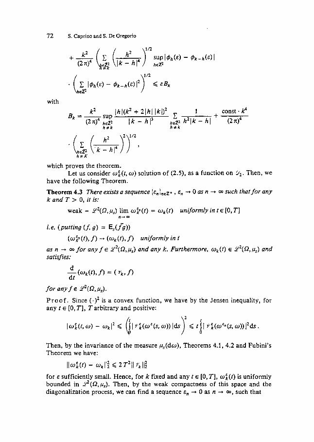
72 S. Caprino and S. De Gregorio
which proves the theorem. Let us consider w f ( t , o) solution of (2.5), as a function on 92. Then, we
have the following Theorem.
Theorem 4.3 There exists a sequence ( E , ) , ~ ~ + , E, -+ 0 as n -. 00 such that for any kand T > 0, it is:
weak - Y~(O,,U,) lim w$(t) = q ( t ) uniformfy in t E [o, TI
i.e. (putting ( A g ) = E , ( f g ) ) (o2(t), f) ---* ( w k ( t ) , f) uniformly in t
as n -+ 00 for any f E Y2(sZ,,us) and any k. Furthermore, ok(t) E Y2(.f2,,u,) and satisfies:
for a n y f c Y~(Q,,u,).
Pro o f . Since ( a ) ’ is a convex function, we have by the Jensen inequality, for any t E [0, TI, T arbitrary and positive:
lo:(f,a) - o k l 2 < SI p / ; ( U E ( S , a ) ) I d r < f j I f ’ ~ ( ~ c n ( S , a ) ) 1 2 d r . c 1 : Then, by the invariance of the measure &do), Theorems 4.1, 4.2 and Fubini’s Theorem we have:
Ilo“kf) - o k l l : 2T211 ’ill; for E sufficiently small. Hence, for k fured and any t E [0, TI, o:(t) is uniformly bounded in Yz(O,,us). Then, by the weak compactness of this space and the diagonalization process, we can find a sequence E, -+ 0 as n -, 00, such that

On the Statistical Solutions of the Two-Dimensional, Periodic Euler Equation 73
( W 2 ( t m , n ( o k ( t m , n
for a n y f ~ -s/5(Q,,us), any k and any tm in a dense set in [0, TI. Analogously, we have: [Ilom - W m 1 1 2 l 2 < 210 - 0 l l v,ll,12
I ( 4 t ) - 4t7,nl G Ilo:(t) - 4 t 7 l l z l l f l l z -
that implies the equicontinuity in t E [0, TI of the functions (ok(t).n,f~ Y2(Q,,u5), since:
This allows to say that the function of time (ok(t),n is continuous in [o,T], for a n y f ~ Y ~ ( Q , , u ~ ) .
Furthermore:
) (o$(t),n = (q,n + j . " $ ( u t n ( 4 ) & f I c
= ( U k , n -k ~(r"z:(oc(s)),nds* 0
Taking the limit as E , + 0, by Theorem 4.2 and the Dominated Con- vergence Theorem, we obtain finally:
I
0 ( u k ( t ) , n = ( u k 3 . f ) + j < )L/k(o(S)),nds
which proves the Theorem.
Acknowledgement
We are pleased to thank M. Pulvirenti, for many useful discussions.
References
[ l ] K a t o . T.: Arch. Rat. Mech. and Anal. 25 (1967) 95 [2) J u d o v i c , V. I . ; Vycis l , 2.: Mat.: Fiz. 3 (1963) (Russian) [3] M a r c h i o r o , C.; P u l v i r e n t i , M.: Commun. Math. Phys. 84 (1982) (41 A l b e v e r i o , S.; R i b e i r o d e F a r i a , M.; H o e g h - K r o h n , R.: J. of Stat. Phys. 20 (1979) [5] B o l d r i g h i n i , C.; F r i g i o , S.: Atti Sem. Mat. Fis. Univ. Modcna, XXVI I (1978) [6] B o l d r i g h i n i , C.; F r i g i o , S.: Commun. Math. Phys. 72 (1980) [7] DUrr, D.; P u l v i r e n t i , M.: Commun. Math. Phys. 85 (1982) [8] N e u n z e r t , H.: Fachb. Math. Univ. Kaiserslautern Preprint 28 (1982). Lecture given at C.I.M.E.
[9] S p o h n , H.: Math. Meth. in the Appl. Sci. 3 (1981) Montecatini (Italy) June 1981
S. Caprino Dipartimento di Maternatica, Universita di Roma "La Sapienza", 00185 Roma, Italy Dipartimento di Matematica, Universita di Camerino 601 32 Camerino, Italy
S. De Gregorio Dipartimento di Matematica, Univcrsita di Roma "La Sapienza", 00185 Roma, Italy Dipartimento di Matematica, Universita de I'Aquila I'Aquila, Italy
(Received January 5, 1984)