on the probability distribution of faults in complex ...on the probability distribution of faults in...

On the Probability Distribution of Faults in Complex

Software Systems

Tihana Galinac Grbac∗

Faculty of Engineering, University of Rijeka, Vukovarska 58, HR-51000 Rijeka, Croatia

Darko Huljenic

Ericsson Nikola Tesla, Krapinska 45, HR-10000 Zagreb, Croatia

Abstract

Context. There are several empirical principles related to the distributionof faults in a software system (e.g. the Pareto principle) widely applied inpractice and thoroughly studied in the software engineering research pro-viding evidence in their favor. However, the knowledge of the underlyingprobability distribution of faults, that would enable a systematic approachand refinement of these principles, is still quite limited.Objective. In this paper we study the probability distribution of faults de-tected during verification in four consecutive releases of a large-scale complexsoftware system for the telecommunication exchanges. This is the first suchstudy analyzing closed software system, replicating two previous studies foropen source software.Method. We take into consideration the Weibull, lognormal, double Pareto,Pareto, and Yule-Simon probability distributions, and investigate how wellthese distributions fit our empirical fault data using the non-linear regres-sion.Results. The results indicate that the double Pareto distribution is themost likely choice for the underlying probability distribution. This is notconsistent with the previous studies on open source software.Conclusion. The study shows that understanding the probability distribu-

∗Corresponding authorEmail addresses: [email protected] (Tihana Galinac Grbac),

[email protected] (Darko Huljenic)

Preprint submitted to Information and Software Technology June 18, 2014

tion of faults in complex software systems is more complicated than previ-ously thought. Comparison with previous studies shows that the fault dis-tribution strongly depends on the environment, and only further replicationswould make it possible to build up a general theory for a given context.

Keywords: software fault distribution, probability distribution, non-linearregression, complex software system, empirical research

1. Introduction

The knowledge of fault distributions in large–scale complex software sys-tems is very important for planning the quality assurance activities. Thereare several empirical principles, widely applied in software development prac-tice, related to the distribution of faults. For example, the Pareto principle[1, 2], also known as the 20-80 rule, is one of the most popular among them.It states that a majority of faults (80%) in a software system is contained ina minority of software modules (20%). There is a lot of empirical evidence infavor of this principle [3, 4, 5, 6, 7, 2, 8, 9, 10]. Another example is the prin-ciple that the minority of modules containing the majority of faults confinesnot too large portion of the system size. Empirical evidence for this principleis obtained in [8, 9, 10].

All such principles ultimately depend on the underlying probability dis-tribution of faults in a software system. However, the converse is not true,that is, the fulfillment of a certain principle does not determine the prob-ability distribution uniquely. For example, there are several distributions,besides the Pareto distribution, that would result in the Pareto principle. Inother words, the empirical evidence in favor of some principle does not implyinformation on the probability distribution, and, indeed, our knowledge onthe probability distribution of faults in software systems is still quite limited.

Recently a lot of attention is put to the more general problem of deter-mining probability distributions of various metrics in software engineering(see e.g. [11, 12, 13]). The final goal of all these works, as well as this paper,is to refine the empirical principles used in software engineering practice,and possibly even use the precise knowledge of probability distributions topredict the behavior of future releases of a complex software system.

The knowledge of the most appropriate probability distribution fittingthe empirical fault data in complex software systems would enable moresystematic approach and refinement of the Pareto principle and other related

2

principles used in the software development practice. This line of thought ispursued in works of Zhang [14] and Concas et al. [15]. Both papers study thefault data for the open source Eclipse system using the non-linear regressionfor fitting.

Zhang [14] compares how the Pareto and Weibull distributions fit thedata, and conclude that the Weibull distribution is significantly better. Asexplained above, this is not contradictory to the Pareto principle itself, sincethe Pareto principle does not imply the underlying probability distribution.

Concas et al. [15] consider the Weibull, lognormal, double Pareto, andYule-Simon distributions. The results reveal that, for the Eclipse system, theYule-Simon distribution provides better fit than the others. The Weibull, log-normal, and double Pareto distributions are quite close, although the Weibulldistribution is the worst in all five considered system releases. The authors ar-gue further in favor of the Yule-Simon, but also lognormal and double Paretodistributions, since they all have a generative model, unlike the Weibull dis-tribution.

Motivated by these two papers on the Eclipse system, and the impor-tance of finding the most appropriate distribution, we study the probabilitydistribution of faults in a very different context, that is, in four consecutivereleases of the large-scale complex software system for telecommunicationexchanges. We consider all distributions appearing in [14] and [15]. Theseare the Pareto, Weibull, lognormal, double Pareto, and Yule-Simon distri-butions. As in [14] and [15], the fitting method is the non-linear regressionfor the fault data in the form of the complementary cumulative distributionfunction (CCDF) of the random variable counting the number of faults in asoftware module.

In reporting the results of non-linear regression we follow closely the expo-sition of [15] to simplify the comparison. Additionally to the goodness-of-fitmeasures, we report the distribution parameters obtained for the best fits.These are not reported in [15], and we can compare only to the Pareto andWeibull distribution fits of [14]. We provide such detailed results, so that thereplications of this study for other software systems could be easily compared.

It turns out that the results are different from those of [14] and [15],which can be explained by a very different context. In our study the doublePareto distribution is the best fit to the fault count data. The lognormaldistribution is the second best, followed closely by the Yule-Simon distribu-tion, which is even slightly better in one of the projects. Only then comesthe Weibull distribution, while the Pareto distribution is worse than others.

3

However, the Pareto distribution performs much better than reported by [14].We hope that this study will become a source of several replications in bothsimilar and different contexts, so that the most appropriate probability dis-tributions of faults could be identified in different types of software systemsand development environments.

The paper is organized as follows. In Section 2 the context of the studyand the fault data are described in detail. Section 3 recalls the consideredprobability distributions. The results of the non-linear regression fit arereported in Section 4. Section 7 concludes the paper.

2. Context of the Study

We describe in this section the context of this study including the softwaresystem, the development organization, the software development process, andthe data collection performed for the purpose of this study.

2.1. Software System

The study is undertaken on a sequence of four development projects,denoted P1, P2, P3, P4, developing consecutive releases of the same softwareproduct. The considered projects are the same as in the study [10], exceptthat the last two releases, denoted by Rel n+3 and Rel n+4, are combinedinto project P4. The reason is that the size of datasets from these two releasesis too small for a reliable fitting, and they are indeed two subprojects of thesame development project.

The software product is the software system for the Mobile Switching Cen-ter (MSC), that is, a functional node in the Third Generation (3G) telecom-munication network. The MSC node is built on Ericsson’s AXE exchangethat has evolved for more than 30 years and is in operation in hundreds ofexchanges all over the world.

The system is coded in Ericsson’s in-house Programming Language forEXchanges (PLEX). It is a large-scale software system with several millionslines of code (LOC). The software system architecture is modular, involvingmore than 1000 software modules.

2.2. Organization

The development organization is a globally distributed Ericsson’s unitwith long experience in software development for AXE exchange. The num-ber of involved development units varied during the projects. A typical

4

Table 1: Project characteristics

Proj.Size Modification No. of No. of No. of No. of Total no.

[kLOC] size [kLOC] modules FT faults ST faults SI faults of faults

P1 2787 736 485 1630 3500 404 5534P2 1793 258 241 835 1693 1051 3579P3 2880 273 295 942 1603 1529 4074P4 1637 265 158 1673 3093 1052 5818

software development project involves more then 300 developers world-wideand lasts for one to two years.

2.3. Development and Verification Process

The software development process has evolved over the years from thetraditional waterfall model by introducing the incremental and iterative de-livery and feature development. In this study we concentrate on the faultsdetected during the testing part of verification process, which consists of thefunction test (FT), system test (ST) and system integration test (SI). Theessential difference is in the system coverage under the test. The functiontest covers functional environment, that is, only software modules responsi-ble for the functional execution and is very often executed in the simulatedsystem environment. The system test covers essential system environmentfor function integration, often executed on the test plants, and the systemintegration test that covers all deployment environment executed on the testplants.

The fault handling process consists of collection of trouble reports (TR)issued whenever the failure occurs. It is very precise and contains all theinformation required for fault analysis and fault decision process. The sameprocess is used during the software verification and during the system inoperation. The fault handling process is a standard Ericsson’s process. TRsare stored in a database, which can be easily searched.

For every failure that occurs during verification, one or more TRs areissued. This is because there could be one or more faults in the code re-sponsible for the same failure. Hence, a TR is issued for each location inthe code (software module) that could contain the fault causing the failure.These TRs are answered, and an answer code is attached to the TR. Theanswer code indicates whether the fault really exists and should be corrected,and whether the fault is already corrected as a consequence of another TR.Duplication of TRs could happen due to parallel testing activities and since

5

Table 2: Module size distributionLOC P1 P2 P3 P4

≤ 5000 307 116 120 455001− 10000 114 74 90 4210001− 20000 42 37 53 5520000− 30000 11 6 10 1130000− 40000 6 3 9 3

> 40001 5 5 13 2

Total 485 251 295 158

the same fault could be a reason for several failures. More precisely, for everyfault in the code there is exactly one TR with the answer code saying thefault should be corrected. Only these TRs are included into our analysis andall duplicates were excluded.

2.4. Data Collection

As a result of the standard TR handling process all relevant data regard-ing TR collection, analyzing and answering are stored in the database.

For the purpose of this analysis, we searched in the database for all TRsreported during function test, system test and system integration test onsoftware modules modified or impacted in the projects. Based on the TRanswer code, we included in our analysis only TRs that need correction,and eliminated the duplicates. This was possible, since the TR answer codeprovides all this information and is easily accessible in the database. Observethat, besides all modules that are modified in a project, we also consider herethose modules that are not modified but contain faults detected in a project.This is in accordance with the original studies [14] and [15]. However, in[10], where the same projects are considered, only modified modules with atleast one fault are taken into account. This explains differences in projectcharacteristics between this study and [10].

The outcome of the data collection in a project are the total and modifiedsize and the number of faults for every software module that was modified orimpacted in that project. The number of software modules, the total size, thesize of modification, the number of faults in every verification phase and thetotal number of faults are given in Table 1 for each project. The module–sizedistribution is given in Table 2.

6

3. Probability Distributions

Let X be the random variable counting the number of faults in a soft-ware module. The empirical data from each of the four considered projectscontains a sample for X. The goal is to study the probability distribution ofX based on these four empirical samples.

We fit the empirical samples for X, as in [13, 14, 15], to the complemen-tary cumulative distribution function (CCDF) of a probability distribution,also known as the survivor function and the reliability function. It is definedat the value x as P (X ≥ x), that is, the probability that the underlyingrandom variable X takes the value greater than or equal to x. As explainedin [13, 15], the CCDF is the key diagram in practice, equivalent to the Albergdiagram, which is the most common diagram used in software engineering.They give a precise relationship between the CCDF and Alberg diagram. Fora detailed discussion of these issues see [16].

The probability density function (PDF) of a probability distribution willbe denoted by p(x). It is defined as the derivative of the cumulative distribu-tion function (CDF), which amounts to the negative derivative of the CCDF.That is,

p(x) = − d

dxP (X ≥ x). (1)

We use PDF to observe the power-law in the tail of considered probabilitydistribution. The exponent α of the power-law tail is defined by the condition

p(x) ∝ x−α (2)

for sufficiently large x. The power-law is best observed in the log-log scale,since the above condition becomes a straight line

ln p(x) = lnC − α lnx, (3)

where C > 0 is the constant of proportionality.In what follows we recall the formulas for PDF and CCDF of the prob-

ability distributions considered in this paper. This material is well-known,but we include it for completeness and to fix the notation for distributionparameters. The notation for parameters of some probability distributionsbelow are adjusted compared to [15], so that the parameter α correspondsto the power-law exponent in the tail.

7

3.1. Weibull Distribution

The Weibull distribution is a continuous probability distribution sup-ported in x > 0. Its CCDF is given as

P (X ≥ x) = exp

(−(x

γ

)β), x > 0, (4)

where β > 0 and γ > 0. Then, the PDF is

p(x) =β

γ·(x

γ

)β−1

· exp

(−(x

γ

)β), x > 0. (5)

In log-log scale the PDF becomes

ln p(x) = ln(β/γβ)− (1− β) ln x− 1

γβeβ lnx, (6)

which contains a power-law with exponent α = 1 − β, but having an extraexponential term in ln x which dominates the behavior.

3.2. Lognormal Distribution

The lognormal distribution is a continuous probability distribution sup-ported in x > 0. It is characterized by the fact that its natural logarithm isthe normal distribution. The mean µ and variance σ2 of the normal distri-bution so obtained are the parameters of the lognormal distribution. Thus,its PDF function is given as

p(x) =1

x√2πσ2

· exp(−(lnx− µ)2

2σ2

), x > 0, (7)

where µ is real and σ > 0. For the CCDF, we have to integrate

P (X ≥ x) =1√2πσ2

·∫ +∞

x

exp

(−(ln t− µ)2

2σ2

)dt

t. (8)

Making the substitution for ln t, and scaling to the standard normal distri-bution (with µ = 0 and σ = 1) yields the CCDF in the form

P (X ≥ x) = 1− Φ

(lnx− µ

σ

), x > 0, (9)

8

where Φ is the CDF of the standard normal distribution. In the log-log scalethe lognormal PDF becomes

ln p(x) = − µ2

2σ2− ln

√2πσ2 −

(1− µ

σ2

)lnx− 1

2σ2(lnx)2 . (10)

This is close to a power-law distribution, having an extra quadratic termin ln x. The coefficient of the linear term is the power-law exponent α =1− µ/σ2.

3.3. Pareto Distribution

The Pareto distribution was originally introduced in [17] to describe thedistribution of income and wealth in a society. It is a continuous probabilitydistribution which is mainly used to fit the tails of other distributions. Inparticular, its support is in x ≥ xm, where xm is certain positive value of therandom variable, usually the beginning of the tail. The Pareto CCDF forx > 0 is given as

P (X ≥ x) =

{1, for 0 < x < xm,(xm/x)

β, for x ≥ xm,(11)

and the PDF

p(x) =

{0, for 0 < x < xm,βxβ

m · x−(1+β), for x ≥ xm,(12)

where β > 0. Clearly, this is a power-law distribution with the exponentα = 1 + β.

We would like to mention here a possible pitfall when fitting the Paretodistribution. Using incorrectly the function (xm/x)

β for all x > 0, instead ofthe CCDF given by (11), would lead to significantly lower goodness-of-fit (seeSection 4). The problem is that this function is not a CCDF of a probabilitydistribution, since it grows to infinity as x approaches zero. In particular,the error of estimate would increase significantly for observations near zero.

Another possibility is to restrict the fitting of the Pareto distributiononly to tail, and discard the body of the distribution. In this approach, theparameter xm is estimated as the beginning of the tail, and then the fittingis performed only in the region x ≥ xm. For more details see [18]. Thisapproach is taken in [13], but not in [15], which we replicate here. Fittingonly the tail certainly increases the goodness-of-fit, as it considers only the

9

region x ≥ xm, but loses all information about the body of the distribution,i.e., x < xm. However, as explained in [13], it is sufficient to make estimates ofsome distribution parameters in future releases, such as the maximal numberof faults in a software unit.

We are making a close replication of [15], in which the approach is to fitthe faults data to the CCDF given by (11) in the full range of a distribution,i.e. not fitting only the tail. Hence, our approach is the same as in [15].

3.4. Double Pareto Distribution

The idea behind the double Pareto class of probability distributions is tofind a distribution that fits well the body of empirical distribution and atthe same time the power-law tail. As in [15], we use the form of the doublePareto distribution developed in [19]. Note that the definition of a power-tailexponent in [19] is a bit different than what we use in this paper. We adjustedthe notation for the double Pareto distribution parameters accordingly.

This double Pareto distribution is a continuous probability distributionsupported in 0 < x ≤ xM , where xM is the maximal possible value of theunderlying random variable. The double Pareto CCDF for x > 0 is given as

P (X ≥ x) =

{1−

[1+(xM/t)−β

1+(x/t)−β

]γ/β, for 0 < x ≤ xM ,

0, for x > xM ,(13)

and the PDF as

p(x) =

γt· [1+(xM/t)−β]

γ/β

[1+(x/t)−β]1+γ/β ·

(xt

)−(1+β), for 0 < x ≤ xM ,

0, for x > xM ,(14)

where 0 < t < xM , β > 0 and γ > 0.The parameter t determines the crossover point x = t, at which the

distribution changes its behavior from the power-law in the body to thepower-law in the tail.

The power-law in the tail is governed by the term (x/t)−(1+β). Indeed, forx sufficiently large (not exceeding xM) with respect to t, we have x/t large,so that the fraction appearing in (14) is approximately equal to 1. Thus, thepower-law exponent in the tail is α = 1 + β.

For the power-law in the body of the distribution, we consider x suf-ficiently small with respect to t, so that x/t is close to zero. For such x

10

the asymptotic behavior of the fraction in equation (14) is proportional to(x/t)β+γ. Multiplying by the last term (x/t)−(1+β) shows that the body fol-lows the power-law with exponent γ − 1.

3.5. Yule-Simon Distribution

The Yule-Simon distribution is the outcome of the so-called preferentialattachment model, developed to explain the power-law in tails of certainempirical distributions. Originally it was developed in [23] to describe dis-tributions of species and genera in the theory of evolution, and later appliedin [21] to the distribution of words in books. It is a discrete probabilitydistribution supported in the non-negative integers.

The Yule-Simon PDF is given as

pk = p0 ·B(c+ k, α)

B(c, α), k = 0, 1, 2, . . . , (15)

where c > 0, α > 0, and 0 < p0 ≤ 1 is the probability that the randomvariable takes the value zero. Here B(a, b) denotes the Beta Function, whichcan be expressed in terms of the Gamma Function as

B(a, b) =Γ(a)Γ(b)

Γ(a+ b). (16)

We only need the values of the Beta Function for a, b > 0, and in that range itis well-defined, that is, there are no poles, and also no zeros. The parameterp0 is in fact determined by c and α by the condition that the total probability∑∞

j=0 pj should be 1. More precisely,

p0 =

(∞∑j=0

B(c+ j, α)

B(c, α)

)−1

, (17)

so that the Yule-Simon PDF is

pk =B(c+ k, α)

B(c, α)·

(∞∑j=0

B(c+ j, α)

B(c, α)

)−1

, k = 0, 1, 2, . . . (18)

The Yule-Simon CCDF is then given as

P (X ≥ x) =∑k≥x

pk

11

= p0∑k≥x

B(c+ k, α)

B(c, α)(19)

=

(∞∑j=0

B(c+ j, α)

B(c, α)

)−1

·∑k≥x

B(c+ k, α)

B(c, α).

It can be shown that the parameter α is the power-law exponent in thetail of the Yule-Simon distribution. Indeed, taking the logarithm of equation(15), and writing the Beta Function as in (16), we obtain

ln pk = C + lnΓ(c+ k)− ln Γ(c+ k + α), (20)

where C = ln p0 + lnΓ(α)− lnB(c, α) is a constant. Applying Stirling’s ap-proximation for the logarithm of the Gamma Function gives, for k sufficientlylarge, that

ln Γ(c+ k)− ln Γ(c+ k + α) ≈

≈ α− ln

(1 +

α

c+ k

)c+k−1/2

− α ln(c+ k + α)

≈ −α ln k. (21)

We used the fact that the second term in the first line tends to −α as k → ∞,while the asymptotic of the last term as k → ∞ coincides with that of−α ln k.Thus, we obtained

ln pk ≈ C − α ln k, (22)

for large k, showing that α is the power-law exponent in the tail.

4. Non-linear Regression Fit

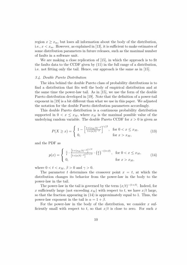
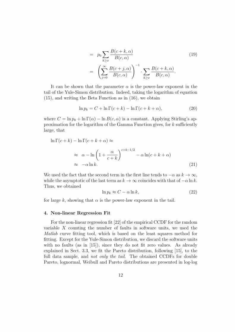
For the non-linear regression fit [22] of the empirical CCDF for the randomvariable X counting the number of faults in software units, we used theMatlab curve fitting tool, which is based on the least squares method forfitting. Except for the Yule-Simon distribution, we discard the software unitswith no faults (as in [15]), since they do not fit zero values. As alreadyexplained in Sect. 3.3, we fit the Pareto distribution, following [15], to thefull data sample, and not only the tail. The obtained CCDFs for doublePareto, lognormal, Weibull and Pareto distributions are presented in log-log

12

Table 3: Distribution parameters and goodness-of-fit for non-linear regressionProject Distribution Parameters R2 Se

P1

Double Pareto

β = 0.7941

0.99901 0.00654γ = 92.5331xM = 142.4923t = 0.0126

Weibullγ = 12.6963

0.98019 0.02926β = 0.7216

Lognormalµ = 2.0034

0.99554 0.01389σ = 1.3623

Paretoxm = 2.4695

0.97077 0.03553β = 0.7436

Yule-Simon (p0 from data)c = 2.0997

0.98179 0.02376α = 1.8212

Yule-Simon (p0 not from data)c = 3.5498

0.99130 0.01643α = 1.9951

P2

Double Pareto

β = 0.7694

0.99759 0.01147γ = 27.3994xM = 124.8392t = 0.0649

Weibullγ = 15.4349

0.98569 0.02797β = 0.7811


0.99610 0.01460σ = 1.3033

Paretoxm = 2.8309

0.96176 0.04572β = 0.7036


0.98159 0.02883α = 1.9281


0.99285 0.01796α = 2.2364

P3

Double Pareto

β = 1.5429

0.99515 0.01789γ = 1.5661xM = 8377.4032t = 8.5373

Weibullγ = 13.2804

0.98436 0.03214β = 0.9589


0.99444 0.01916σ = 1.0944

Paretoxm = 2.8945

0.95798 0.05268β = 0.7898


0.96888 0.03945α = 2.0078


0.98967 0.02273α = 2.6396

P4

Double Pareto

β = 0.9672

0.99703 0.01347γ = 2.7293xM = 2942.2168t = 3.3279

Weibullγ = 22.2033

0.97342 0.04029β = 0.7237


0.99295 0.02075σ = 1.4433

Paretoxm = 3.6015

0.97523 0.03810β = 0.6280


0.98353 0.03100α = 2.9207


0.99709 0.01302α = 2.1426

13

scale in Fig. 1 for project P1, Fig. 2 for project P2, Fig. 3 for project P3,Fig. 4 for project P4, and the parameter values are listed in Table 3.

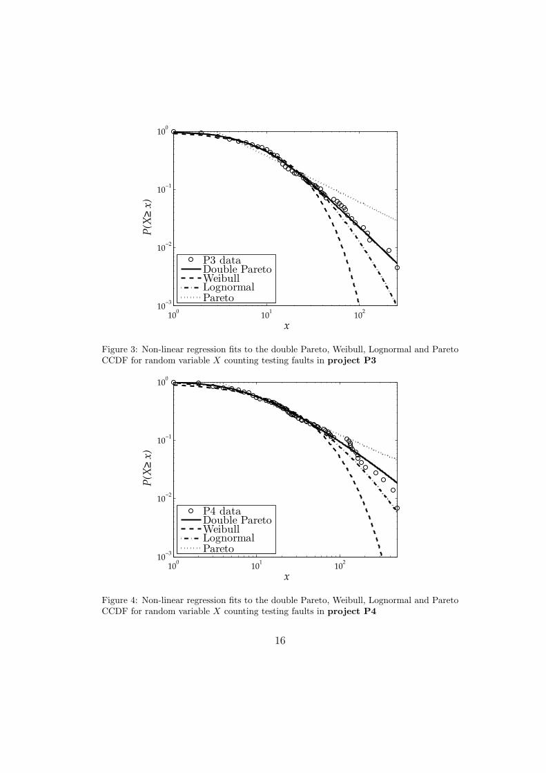
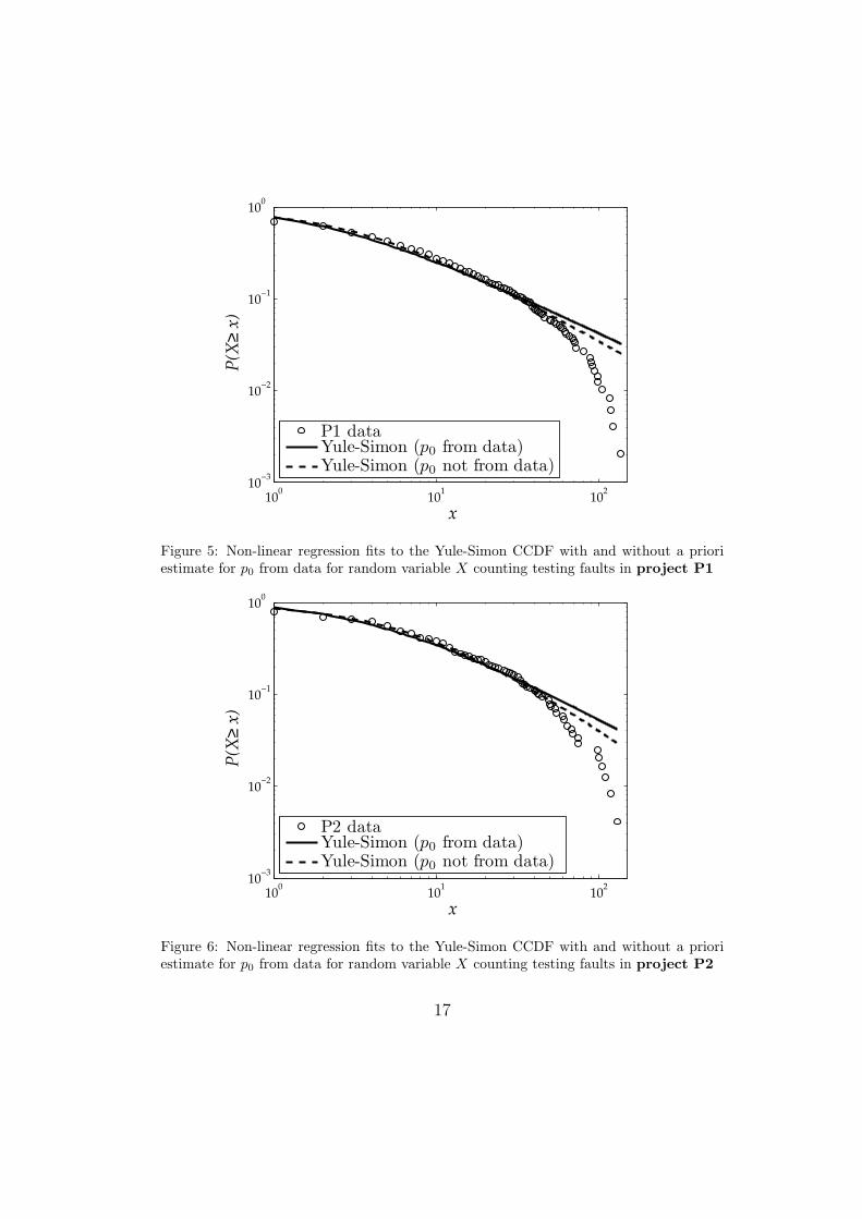
Fitting the Yule-Simon distribution is done in two ways. The first wayis to estimate p0 a priori as the relative frequency of software units with nofaults in the sample. This approach was taken in [15]. The second way is toexpress p0 in terms of parameters c and α, as in equation (17), and then fitto the CCDF given by formula (19). The obtained CCDFs for Yule-Simondistributions are presented in log-log scale in Fig. 5 for project P1, Fig. 6for project P2, Fig. 7 for project P3, Fig. 8 for project P4, and the values ofdistribution parameters in Table 3.

As a measure for goodness-of-fit we compute, as in [14], the coefficient ofdetermination R2 adjusted for the degrees of freedom of the fitting model,and the standard error of estimate Se. Their values are also given in Table3.

More precisely, let

SSerr =n∑

i=1

(yi − yi)2 (23)

be the sum square error, where yi and yi are the actual and fitted values of ithobservation, and n is the number of observations. The least square methodused in non-linear regression actually determines the unknown parametersby minimizing this value. Let

SStot =n∑

i=1

(yi − y)2 (24)

be the total sum of squares, where y is the mean of the observed data.The adjusted coefficient of determination R2 is defined as

R2 = 1− (n− 1)SSerr

(n−m− 1)SStot

, (25)

where m is the number of parameters in the fitting function.The standard error of estimate Se is defined as the square root of the sum

square error divided by the degrees of freedom. That is,

Se =

√SSerr

n−m. (26)

14

100

101

102

10−3

10−2

10−1

100

x

P(X

≥ x

)

P1 dataDouble ParetoWeibullLognormalPareto

Figure 1: Non-linear regression fits to the double Pareto, Weibull, Lognormal and ParetoCCDF for random variable X counting testing faults in project P1

100

101

102

10−3

10−2

10−1

100

x

P(X

≥ x

)



15

100

101

102

10−3

10−2

10−1

100

x

P(X

≥ x

)



100

101

102

10−3

10−2

10−1

100

x

P(X

≥ x

)



16

100

101

102

10−3

10−2

10−1

100

x

P(X

≥ x

)

P1 dataYule-Simon (p0 from data)Yule-Simon (p0 not from data)

Figure 5: Non-linear regression fits to the Yule-Simon CCDF with and without a prioriestimate for p0 from data for random variable X counting testing faults in project P1

100

101

102

10−3

10−2

10−1

100

x

P(X

≥ x

)



17

100

101

102

10−3

10−2

10−1

100

x

P(X

≥ x

)



100

101

102

10−3

10−2

10−1

100

x

P(X

≥ x

)



18

Comparing the goodness-of-fit reported in Table 3 shows first of all thatthe R2 values for all distributions are very close. The difference of the coeffi-cient R2 between the best and the worst fit for each project does not exceed0.04. However, there is a certain tendency that can be observed in all theprojects.

The double Pareto distribution has the highest R2 in projects P1, P2 andP3, while in P4 the R2 for the Yule-Simon distribution (with p0 not estimatedfrom the data) is better, but only for negligible 0.00005. Hence, we concludethat the most appropriate probability distribution to fit our empirical datais the double Pareto distribution.

Despite the Yule-Simon outperforming slightly the lognormal distributionin P4 (for 0.004), the lognormal distribution has consistently higher valuesof R2 in P1, P2 and P3. Hence, it is more likely that the lognormal is thesecond best choice for the fit, followed by the Yule-Simon distribution (withp0 not estimated from the data).

Only then comes the Weibull distribution, with higher values of R2 thanfor the Pareto distribution in P1, P2 and P3, although slightly outperformedby the Pareto distribution in P4 (for less than 0.002).

These results are not consistent with those of [15], which point to theYule-Simon distribution as significantly better fit than others. The reason forthis inconsistency is certainly a very different context of this study comparedto the previous work. It is also interesting to observe that the Weibull andPareto distributions are much closer than obtained in [14].

5. Discussion and future work

The detailed discussion in Section 4 of the goodness-of-fit using the non-linear regression for the five considered probability distributions is summa-rized in Table 4. In the same table we also summarize the results of [15] and[14]. This is a bit simplified view of the results, as there is no quantitativeinformation.

Widely used empirical principles on fault distributions, originally stud-ied in [8], and in further replicated studies [9] and [10], are related to thePareto principle of fault distribution, persistence of faults across the veri-fication phases, effects of module size and complexity on fault proneness.Although the empirical Pareto principle has been confirmed in number ofdifferent contexts and studies it does not imply that the underlying statis-tical fault distributions are equal. In fact, the results in Table 4 show that,

19

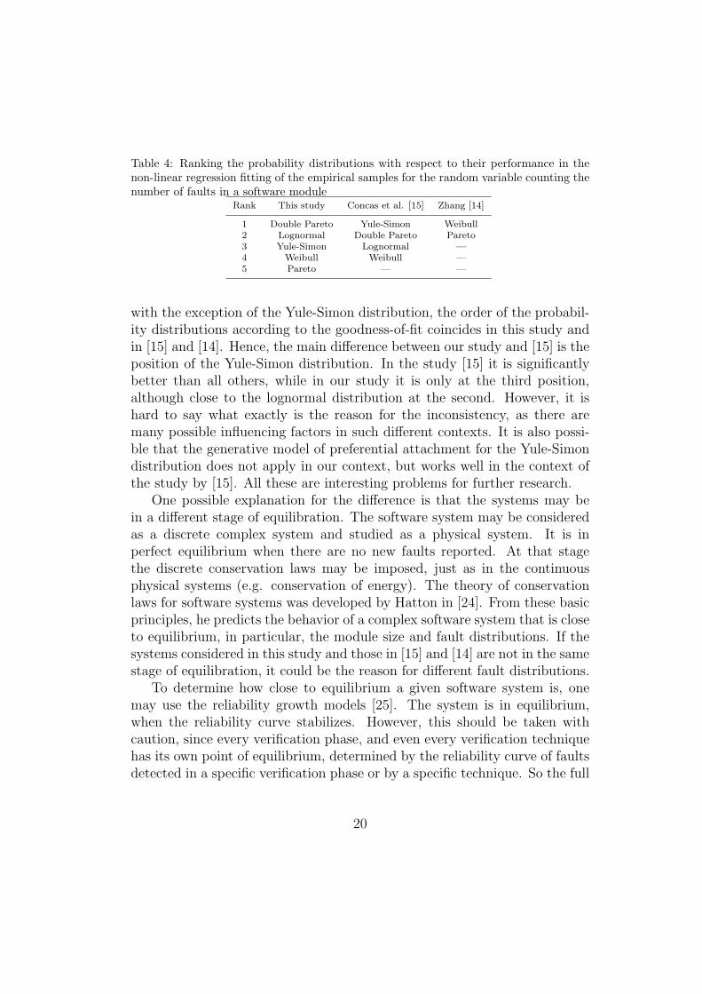
Table 4: Ranking the probability distributions with respect to their performance in thenon-linear regression fitting of the empirical samples for the random variable counting thenumber of faults in a software module

Rank This study Concas et al. [15] Zhang [14]

1 Double Pareto Yule-Simon Weibull2 Lognormal Double Pareto Pareto3 Yule-Simon Lognormal —4 Weibull Weibull —5 Pareto — —

with the exception of the Yule-Simon distribution, the order of the probabil-ity distributions according to the goodness-of-fit coincides in this study andin [15] and [14]. Hence, the main difference between our study and [15] is theposition of the Yule-Simon distribution. In the study [15] it is significantlybetter than all others, while in our study it is only at the third position,although close to the lognormal distribution at the second. However, it ishard to say what exactly is the reason for the inconsistency, as there aremany possible influencing factors in such different contexts. It is also possi-ble that the generative model of preferential attachment for the Yule-Simondistribution does not apply in our context, but works well in the context ofthe study by [15]. All these are interesting problems for further research.

One possible explanation for the difference is that the systems may bein a different stage of equilibration. The software system may be consideredas a discrete complex system and studied as a physical system. It is inperfect equilibrium when there are no new faults reported. At that stagethe discrete conservation laws may be imposed, just as in the continuousphysical systems (e.g. conservation of energy). The theory of conservationlaws for software systems was developed by Hatton in [24]. From these basicprinciples, he predicts the behavior of a complex software system that is closeto equilibrium, in particular, the module size and fault distributions. If thesystems considered in this study and those in [15] and [14] are not in the samestage of equilibration, it could be the reason for different fault distributions.

To determine how close to equilibrium a given software system is, onemay use the reliability growth models [25]. The system is in equilibrium,when the reliability curve stabilizes. However, this should be taken withcaution, since every verification phase, and even every verification techniquehas its own point of equilibrium, determined by the reliability curve of faultsdetected in a specific verification phase or by a specific technique. So the full

20

system is in equilibrium only after all verification stages and techniques arestabilized. Hence, an important line of further research is to study the faultdistributions in each verification phase. On the other hand, if a system isproduced evolutionary in a sequence of releases as the system in this study,it would be interesting to observe the existence of the equilibrium point fromthe system evolution perspective.

Another factor that could be the reason for different results here com-pared to the previous studies is the module size distribution of the observedsystem. The connection between fault distribution and module sizes wasalready studied in the pioneering work [26]. The linear correlation betweenfaults and size is also one of the hypothesis considered in [8, 9, 10], but it wasonly partially confirmed. The size distribution for software systems close toequilibrium, as a consequence of the conservation laws was also studied in[24]. As explained in previous section 2.1, the projects in this study are thesame as in [10], and a rough distribution of module sizes is given in Table 2.It turns out that the size distribution in project P4 is quite different than inother projects considered here. It has significantly higher portion of largermodules (10–20 kLOC). On the other hand, observe that the order of bestfit fault distributions for project P4 is a bit different than for other projects,close to the order reported in [15]. In particular, the Yule-Simon distri-bution fits the fault data for project P4 equally well as the double Paretodistribution. It could be possible that the generative model of preferentialattachment giving the Yule-Simon distribution depends on the size distribu-tion. Unfortunately, only the total system size is reported in [15] and [14],so that we cannot verify this conjecture.

6. Threats to validity

Internal validity refers to a proper demonstration of a casual relationbetween two variables in a study. In our case, there are two possible threatsto internal validity, which are the same as in the original studies [14] and[15]. As we follow the original studies in using the non-linear regression tofit the fault data, the first threat to internal validity is a possibility thatthe obtained distribution fits do not reflect the underlying distribution offaults and are just obtained by chance. Very high R2 value assures thatthis is not the case. Another possibility to verify this would be distributionfitting using the maximum likelihood method, combined with Monte Carlosimulation for evaluating the distribution fits. The second threat to internal

21

validity is that, even though the distribution is correct, it is not a consequenceof its generative model, when such model exists. This is a difficult question,which was neither pursued here, nor in the original studies [14] and [15],except that in the latter the very existence of a generative model for theYule-Simon distribution was taken as an additional argument in its favor.The same holds for the double Pareto distribution, which is the best fit inthis study.

The construct validity refers to whether the particular properties of thesamples in a study are measures of general constructs. The question is towhich extent the sample projects studied in this paper represent the devel-opment project of the considered system. Reducing the threat to constructvalidity is the reason for using four projects on the same system. Note thatduring this four projects the development organization have changed as ex-plained in the Section 2.2 although the real faults for each release, representedin figures of Section 4, seem to have visually almost the same behavior. Itturns out that the double Pareto distribution is, indeed, the best fit in allthe projects. However, the distribution parameters are varying, so that thecomplete understanding of the construct would require further estimationmodels for parameter changes. This difficult issue is out of scope of thiswork. It is possible that the reason is in a different size distribution. Theresults may also be influenced by the differences in data collection. The datacollection for this study is described in Section 2. It relies on the data fromtrouble reports, which is very precise and linked to the system module at themoment of fault detection and during correction. The data collection for theEclipse system in the previous study relies on the open bug report database,in which it is not so easy to relate faults with modules, eliminate duplicationsand false trouble reports.

External validity refers to the generality of the results across different set-tings including those not considered in a study. This replication study is anattempt to generalize the findings of the original studies on fault distributions[15] and [14]. In this replication study we analyzed the fault distributions inan industrial context, which is quite different from the open source develop-ment environment in the original studies. Thus, addressing the threat to theexternal validity is the main focus of this paper. It turns out that the resultsare different than in the original studies, and possible reasons for that arediscussed in Sect. 5.

22

7. Conclusion

Building a software engineering theory of fault distributions has recentlyreceived significant attention. So far, we are aware of empirical principlesregarding fault distributions that have been empirically confirmed in differ-ent environments. However, knowing the appropriate statistical fault dis-tribution would enable more systematic approach for software engineeringmanagement practice. Then we could move a step forward in the softwareengineering research. One direction would be to a more general level, thatis, looking for the underlying processes that generate distributions and howthey influence the statistical fault distributions, and thus, finally start tobuild systematic theory of fault distributions. Another direction would betowards prediction of fault distribution early in development projects, thatis, constructing parameter estimation models for the underlying distribution.

This paper contributes to the study of software fault distributions byreplicating the studies [15] and [14] in the context of a commercial large-scalecomplex software system developed by a globally distributed organizationusing strictly defined development processes. This is very different contextthan the open source projects considered in the original studies, and it turnsout that the results are different. A high-level discussion of some possiblefactors influencing different fault distribution in this and original studies isprovided in Section 5.

However, to determine exactly the factors controlling the fault distribu-tion in complex software systems, it is necessary to gather more informationin similar and different contexts, and if possible conduct controlled exper-iments with the aim to study the fault distributions. We hope that thisstudy will become a source of replications leading to better understandingof the probability distribution of faults in complex software systems. Thiswould provide invaluable insight, and enable more systematic approach andrefinement of the empirical principles regarding fault distributions used inthe software development practice, as well as possible predictions of systembehavior for future releases.

Acknowledgment

The work presented in this paper is supported by the University of Rijekaresearch grant 13.09.2.2.16.

23

References

[1] J. Juran, Quality control handbook, McGraw-Hill, New York, 1974.

[2] N. Ohlsson, H. Alberg, Predicting fault-prone software modules in tele-phone switches, IEEE Trans. Softw. Eng. 22 (1996) no. 12, 886–894.

[3] B. Compton, C. Withrow, Prediction and control of ADA software de-fects, J. Syst. Softw. 12 (1990) no. 3, 199–207.

[4] G. Denaro, M. Pezze An empirical evaluation of fault-proneness models,in: Proc. 24th Internat. Conf. on Softw. Eng. (ICSE ’02), pp. 241–251.

[5] M. English, C. Exton, I. Rigon, B. Cleary, Fault detection and predictionin an open-source software project, in: Proc. 5th Internat. Conf. onPredictor Models in Softw. Eng. (PROMISE ’09), pp. 17:1–17:11.

[6] M. Kaaniche, K. Kanoun, Reliability of a commercial telecommunica-tions system, in: Proc. 7th Internat. Symp. on Softw. Reliability Eng.(ISSRE ’96), pp. 207–212.

[7] J. Munson, T. Khoshgoftaar, The detection of fault-prone programs,IEEE Trans. Softw. Eng. 18 (1992) no. 5, 423–433.

[8] N. Fenton, N. Ohlsson, Quantitative analysis of faults and failures ina complex software system, IEEE Trans. Softw. Eng. 26 (2000) no. 8,797–814.

[9] C. Andersson, P. Runeson, A replicated quantitative analysis of faultdistributions in complex software systems, IEEE Trans. Softw. Eng. 33(2007) no. 5, 273–286.

[10] T. Galinac Grbac, P. Runeson, D. Huljenic, A second replicated quanti-tative analysis of fault distributions in complex software systems, IEEETrans. Softw. Eng. 39 (2013) no. 4, 462–476.

[11] G. Concas, M. Marchesi, S. Pinna, N. Serra, Power-laws in a largeobject-oriented software system, IEEE Trans. Softw. Eng. 33 (2007) no.10, 687–708.

[12] P. Louridas, D. Spinellis, V. Vlachos, Power laws in software, ACMTrans. Softw. Eng. and Methodology 18 (2008) no. 1, article no. 2.

24

[13] G. Concas, M. Marchesi, A. Murgia, R. Tonelli, An empirical study ofsocial network metrics in object-oriented software, Advances in Softw.Eng., vol. 2010, Article ID 729826, 21 pages, 2010.

[14] H. Zhang, On the distribution of software faults, IEEE Trans. Softw.Eng. 34 (2008) no. 2, 301–302.

[15] G. Concas, M. Marchesi, A. Murgia, R. Tonelli, I. Turnu, On the distri-bution of bugs in the Eclipse system, IEEE Trans. Softw. Eng. 37 (2011)no. 6, 872–877.

[16] M. E. J. Newman, Power laws, Pareto distributions and Zipf’s law,Contemporary Physics 46 (2005), no. 5, 323–351.

[17] V. Pareto, Cours d’economie politique, F. Rouge, Lausanne, 1897.

[18] A. Clauset, C. R. Shalizi, M. E. J. Newman, Power-law distributions inempirical data, SIAM Review 51 (2009) no. 4, 661–703.

[19] C. Stark, N. Hovius, The characterization of landslide size distributions,Geophysical Research Letters 28 (2001) no. 6, 1091–1094.

[20] G. Yule, A mathematical theory of evolution based on the conclusionsof Dr. J. C. Willis, Philosophical Trans. Royal Soc. of London Series B213 (1925), 21–87.

[21] H. Simon, On a class of skew distribution functions, Biometrika 42(1955), 425–440.

[22] D. Bates, D. Watts, Nonlinear regression analysis and its applications,John Wiley & Sons, New York, 1988.

[23] G. Yule, A mathematical theory of evolution based on the conclusionsof Dr. J. C. Willis, Philosophical Trans. Royal Soc. of London Series B213 (1925), 21–87.

[24] L. Hatton, Power-Law Distributions of Component Size in General Soft-ware Systems IEEE Trans. Softw. Eng. 35 (2009) no. 4, 566–572.

[25] Lyu MR (ed) Handbook of software reliability engineering, McGraw-Hill, New York, 1996.

25

[26] V.R. Basili and B.T. Perricone, Software Errors and Complexity: anEmpirical Investigation, Commun. ACM, 27 (1984), no. 1, 42–52.

26

on the probability distribution of faults in complex ...on the probability distribution of faults in...

Documents