On the Passive Dynamics of Quadrupedal Running

Ioannis Poulakakis

Department of Mechanical Engineering

McGill University, Montreal, Canada

A thesis submitted to the Faculty of Graduate Studies and Research in partial

fulfillment of the requirements of the degree of

Masters of Engineering

Ioannis Poulakakis, July 2002

Abstract

In this thesis, the dynamics of quadrupedal running via the bounding gait is

studied. To analyse the properties of the passive dynamics of Scout II, a model

consisting of a body and two massless spring-loaded prismatic legs is introduced.

A return map is derived to study the existence of periodic system motions.

Numerical studies of the return map show that passive generation of cyclic motion

is possible. Most strikingly, local stability analysis of the return map shows that

the dynamics of the open loop passive system alone can confer stability of the

motion. Stability improves at higher speeds, a fact which is in agreement with

recent results from Biomechanics showing that the dynamics of the body become

dominant in determining stability when animals run at high speeds. Furthermore,

pronking is found to be more unstable than bounding, which explains why Scout

II shows a “preference” for the bounding gait. These results can be used in

developing a general control methodology for legged robots, resulting from the

synthesis of feed-forward and feedback models that take advantage of the

mechanical system.

ii

Résumé

Cette thèse examine la dynamique d'un système quadrupède qui posséde une

démarche de bondissement. Pour analyser les propriétés de la dynamique passive

de Scout II un modèle se composant d'un corps et de deux jambes prismatiques à

ressort sans masse est présenté. Une carte de retour est dérivée pour étudier

l'existence des mouvements périodiques du système. Les études numériques de la

carte de retour prouvent que la génération passive du mouvement cyclique est

possible. L'analyse locale de stabilité de la carte de retour prouve que seul la

dynamique du système passif sans rétroaction peut conférer stabilité du

mouvement. La stabilité s'améliore à des vitesses plus élevées, un fait qui est en

accord avec des résultats récents Biomécanique que la dynamique du corps

devient dominante dans la détermination de la stabilité quand les animaux

fonctionnent aux vitesses élevées. En outre, pronking s'avère plus instable que le

bondissement, qui explique pourquoi Scout II montre une préférence pour la

démarche de bondissement. Ces résultats et la synthèse des modèles alimenter

vers l'avant et de rétroaction peuvent être employés en développant une

méthodologie générale de commande pour les robots ambulatoire.

iii

Acknowledgments

Throughout the course of my research at CIM, I have had the opportunity to meet

and work with exceptional people, to whom I would like to express my deepest

appreciation. Particularly, I would like to thank:

• My supervisors, Professors Martin Buehler and Evangelos Papadopoulos, for

their professional guidance and constant encouragement throughout the course

of this investigation. Their superb knowledge of Robotics and Legged

Locomotion in particular was an irreplaceable resource during the course of

my research.

• James Smith, a valuable friend and colleague in the Scout II project, for his

selfless assistance. His excellent understanding of software and hardware and

his ability in solving practical problems have been crucial in bringing Scout

back to life. He has literally been my third supervisor.

• Ioannis Rekleitis and Louiza Solomon not only for helping me in the first days

of my stay in Montreal (“Good morning, I’m looking for an apartment”), but

also for making sure that my life in this city has also a “non-lab” component.

• Evgeni Kiriy, for maintaining the ARL computer network and for many

“philosophical” discussions during many of those sleepless nights in the lab.

• Dave McMordie for encouraging me to do hands-on work in the lab. I truly

admire his amazing talent in designing and performing experiments and his

intuitive understanding of any electromechanical device.

• Don Campbell for his valuable (twenty four hours per day) help in

understanding basic concepts in software and hardware. Also for making sure

iv

that I would participate in the early sessions at the CNM symposium at the

University of Michigan.

• Matt Smith, Chris Prahacs and Enrico Sabeli for their valuable assistance

towards a better mechanical design of our robot.

• Carl Steeves, for being a valuable team member in many course projects that I

took at McGill and for his selfless assistance in understanding the (many)

“mysteries” of WM 2D.

• Christine Georgiadis, the other Greek ARL member, for proof reading

portions of my thesis.

• Ned Moore, for always being willing to help and give advice. Also for his

assistance during my first steps in the MicroP course.

• Shervin Talebi, for introducing me to the magical world of Scout II and for

being patient in answering all my questions about the robot.

• Aki Sato for being the other ARL night-shift co-worker. Also for making

valuable recommendations in the modeling chapter of my thesis.

• Gen Vinois, our lab administrator, for making our life easier in ARL, by

keeping the paperwork away and allowing us to concentrate on our research.

• Jan Binder and Danny Chouinard, CIM’s systems administrators, for keeping

the computers at CIM running smoothly. Also for saving me from a few

unexpected deletings of valuable MATLAB code.

• The CIM administrating stuff: Marlene Gray and Cynthia Davidson and the

Mechanical Engineering graduate secretary Anna Cianci for their advice on

how to cope with the McGill bureaucracy (banner) and its countless deadlines.

• Kostas Karagkiozis for his friendship and valuable advice. Also for his help in

getting a visa for the US.

• The Greek-Italian Hurley’s team: Greg Aloupis, Giorgos Rekleitis and Alessio

Salerno for all the fond memories.

• Most of all I am grateful to my family that supported me any time I was in

need, always standing by me, guiding me into searching for answers and

striving for a better tomorrow.

v

Table of Contents

Abstract.................................................................................................................. ii

Résumé .................................................................................................................. iii

Acknowledgments .................................................................................................iv

Table of Contents ..................................................................................................vi

List of Figures..................................................................................................... viii

1. Introduction........................................................................................................1

1.1. Overview...................................................................................................... 1

1.2. Motivation.................................................................................................... 3

1.3. Background and Literature Survey .............................................................. 4

1.3.1. Dynamically Stable Legged Machines ................................................4

1.3.2. Models for Legged Locomotion ..........................................................7

1.3.3. Dynamic Stability Analysis ...............................................................11

1.3.4. Passive Dynamics ..............................................................................15

1.4. Previous Work in ARL .............................................................................. 19

1.5. Thesis Contributions and Organisation...................................................... 23

2. Scout II Bounding Models for Analysis and Simulation ..............................25

2.1. Introduction................................................................................................ 25

2.2. Running Gaits and Locomotion Models .................................................... 26

2.3. Notation and Assumptions ......................................................................... 31

2.4. SLIP Dynamics .......................................................................................... 34

2.5. Scout II Dynamics...................................................................................... 37

2.5.1. Double Leg Flight Phase ...................................................................40

2.5.2. Back Leg Stance Phase......................................................................41

vi

2.5.3. Double Leg Stance Phase ..................................................................45

2.5.4. Front Leg Stance Phase .....................................................................48

2.5.5. Phase Transition Events.....................................................................51

2.6. Scout II Drive Dynamics............................................................................ 53

2.6.1. Battery Model ....................................................................................53

2.6.2. Motor/Amplifier Model.....................................................................54

2.7. Simulation Environments........................................................................... 58

3. Passive Dynamics of Scout II: Methods .........................................................62

3.1. Introduction................................................................................................ 62

3.2. Poincaré Map: A Useful Tool for Analysis ............................................... 63

3.3. Self-Stabilised Passive Running in SLIP ................................................... 68

3.4. Existence of a Passive Bounding Gait ....................................................... 75

3.4.1. Definition of the Bounding Return Map............................................76

3.4.2. Searching for Fixed Points ................................................................81

3.4.3. Finding Fixed Points..........................................................................83

4. Passive Dynamics of Scout II: Results ...........................................................88

4.1. Introduction................................................................................................ 88

4.2. Symmetric Periodic Trajectories................................................................ 89

4.3 Stability Analysis ........................................................................................ 96

5. Conclusions and Future Research................................................................104

5.1. Conclusions.............................................................................................. 105

5.2. Future Recommendations ........................................................................ 106

Bibliography .......................................................................................................109

A.Cartesian Dynamics .......................................................................................117

vii

List of Figures

Fig 1.1. The first actively balanced legged robots built by M. Raibert and

his co-workers: The 2D (left) and the 3D (right) hoppers, [40]. .............5

Fig. 1.2. The MIT leg lab’s biped (left) and quadruped (right) robots, [40]. ........6

Fig. 1.3. Patrush I, II and Tekken; Prof. H. Kimura, [79]......................................7

Fig. 1.4. Models for walking and running in the sagittal and horizontal

plane: Inverted pendulum (IP), Spring Loaded Inverted Pendulum

(SLIP) and Lateral Leg Spring (LLS). ....................................................9

Fig. 1.5. Monopod II (left), and Scout I (right). ..................................................20

Fig. 1.6. Scout II with compliant legs (left) and lockable passive knees

(right). ....................................................................................................22

Fig. 1.7. RHex in rough terrain and on stairs.......................................................22

Fig. 2.1. Gait diagrams showing the pattern of leg use in different running

gaits. Shaded areas represent legs that are on the ground while

blank areas represent legs that are in the air. Indexes: L for Left,

R for Right, F for Front and B for Back. ...............................................28

Fig. 2.2. The concept of virtual legs for the bounding gait..................................29

Fig. 2.3. The two-dimensional model for Scout II in the sagittal plane. .............30

Fig. 2.4. Snapshots of the robot at different phases and events triggering

each phase..............................................................................................31

Fig. 2.5. Spring Loaded Inverted Pendulum (SLIP): A template for

running. Mechanical parameters and variables with sign

conventions............................................................................................34

Fig. 2.6. Symbols and sign conventions for the variables describing

Scout’s planar model. ............................................................................39

viii

Fig. 2.7. Scout II in the back leg stance phase.....................................................42

Fig. 2.8. Scout II in the double leg stance phase. ................................................46

Fig. 2.9. Scout II in the front leg stance phase.....................................................48

Fig. 2.10. Battery Model: Resistor in series with an ideal voltage source.............53

Fig. 2.11. Top: Voltage measured in the experiment (blue line) and voltage

calculated (red line) using Eq. (2.50). Bottom: Current measured

in the experiment. ..................................................................................54

Fig. 2.12. Two motor/amplifier blocks in parallel with the battery:

Amplifiers operate in current mode (top) and amplifiers operate in

saturation mode (bottom). .....................................................................55

Fig. 2.13. Four quadrant motor characteristic curves. ...........................................58

Fig. 2.14. Scout II planar model built in Working Model 2D............................60

Fig. 3.1. Solution curve and orbit of a two dimensional dynamical system........65

Fig. 3.2. The definition of a Poincaré map: Cross section Σ and map ...........66 P

Fig. 3.3. The Spring Loaded Inverted Pendulum model: A template for

running...................................................................................................69

Fig. 3.4. Passive convergence to a stable running cycle in the SLIP...................71

Fig. 3.5. Leg angle and leg length for the conditions of Fig. 3.4.........................71

Fig. 3.6. Smaller touchdown angles (up) cause the system to accelerate by

decreasing its hopping height while larger touchdown angles

(bottom) cause the system to decelerate by increasing its hopping

height. ....................................................................................................72

Fig. 3.7. Forward speed at convergence versus touchdown angle at fixed

points obtained for initial forward speeds from 5m/s to 7m/s and

for an apex height equal to 1m. .............................................................74

Fig. 3.8. A passive and conservative model for Scout II. ....................................77

Fig. 3.9. Flow chart presenting the numerical algorithm for calculating the

fixed points of the return map. ..............................................................84

Fig. 3.10. Evolution of the state variables during one bounding cycle. The

vertical lines show the events: back leg touchdown, front leg

touchdown, back leg lift-off and front leg lift-off. ................................85

ix

Fig. 3.11. Evolution of the leg length and the leg angles. .....................................86

Fig 4.1. Fixed points for 1m/s forward speed and 0.35m apex height................92

Fig. 4.2. Snapshots showing the motion of Scout II for the internal branch

and the external branch fixed points. The plot on the left is a

smaller version of Fig. 4.1. ....................................................................93

Fig. 4.3. Formations of fixed points for apex height 0.35 m and forward

speeds to 1.5 m/s. [ ]min max,E E is the range of the total energy of

the fixed points. .....................................................................................93

Fig 4.4. Formations of fixed points for apex height 0.35m and speeds

varying from 1.5 to 3.5 m/s. ..................................................................94

Fig. 4.5. Constant energy levels for energies between 70J and 200J. The

markers are the fixed points found at speeds from 1.5 to 3.5 m/s. ........95

Fig. 4.6. Root locus showing the paths of the four eigenvalues as the pitch

rate varies from low values (blue) to high values (red). The same

pattern is observed for different forward speeds and apex heights. ......98

Fig. 4.7. Norm of the larger eigenvalue at various pitch rates and for

forward speeds between 1.5 and 4m/s. The apex height is 1m. ..........100

Fig. 4.8. Norm of the larger eigenvalue at various pitch rates and for apex

heights between 0.32 and 0.37m. The forward speed is 3m/s. ............101

Fig. 4.9. The concept of dimensionless moment of inertia. The ground

force applied at the left foot causes the right hip (a) not to move at

all, (b) to move downwards, or (c) to move upwards..........................103

x

Η παρούσα εργασία αφιερώνεται στους γονείς µου.

xi

Chapter 1

Introduction

1.1. Overview

Robotics constitutes a relatively young branch of science and technology, which

is devoted to studying and developing machines that have the ability to interact

with their environment. Indeed, robots execute tasks that are governed not only by

a set of rules relative to the internal structure and operation of the machine itself,

but also by rules that are imposed by the interaction between the machine and its

environment. The goal of robotics is to construct machines that can replace human

beings in the execution of a task, as regards both physical activity and decision-

making. The above consideration points out the conceptual and technological

complexity that influences the development of robots endowed with good

characteristics of autonomy. This is needed in the execution of missions in

unstructured or scarcely structured environments, i.e. when geometrical or

physical description of the environment is not completely known a priori.

The field of mobile robotics is concerned with studying robots with

marked characteristics of autonomy, whose applications are conceived to solve

problems of operation in hostile environments (space, underwater, nuclear,

military, etc) or to execute service missions (domestic applications, medical aids,

assistant to the disabled, agriculture, etc) is still in its infancy. Most of the mobile

robots that have been designed and built up to now use wheels for locomotion.

This is a consequence of the inherent static stability and power efficiency of

wheeled mobile robots, which made them an attractive first step for practical

1

applications. However, wheels and tracks have limitations when it comes to

negotiating uneven terrain or climbing steps.

Mobility is one of the most important reasons for exploring the use of legs

in locomotion. Indeed, in spite of impressive improvements of wheeled and

tracked vehicles, their mobility is still far from the mobility of animals. Wheels

and tracks excel on prepared surfaces such as rails and roads, but most places

have not yet been paved (fortunately). Only about half the earth’s landmass is

accessible to existing wheeled and tracked vehicles, [62], whereas animals on foot

can reach a much larger fraction!

The most important difference between wheeled and legged platforms lies

in the fact that wheeled vehicles require a continuous path of support. This is in

contrast with machines that use legs for locomotion, which can propel using series

of isolated footholds allowing them to traverse irregular terrains. Legs also

provide an active suspension that decouples the path of the body from the path of

the feet. Thus the performance of legged vehicles can, to a certain extend, be

independent of the detailed ground profile. This decoupling property can be

exploited by a legged system to increase its speed and efficiency on rough terrain.

Two of the key points in designing reliable legged robots are stability and

power efficiency. Trying to improve stability, many researchers develop legged

machines that are statically stable, having at least three legs on the ground at the

same time, while maintaining their centre of mass in the tripod formed by these

legs. Moreover, static stability requires velocities and accelerations to be

sufficiently small such that inertia effects do not disturb motion’s stability.

Statically stable legged robots usually have a high number of legs and use many

actuators per leg. This fact significantly limits the number of behaviours,

increases weight, deteriorates energy efficiency and finally, it can result in low

speeds, poor reliability and high costs.

Unlike statically stable robots, dynamically stable robots can tolerate

departures of the centre of mass from the support polygon formed by the legs in

contact with the ground. A legged system that balances actively is allowed to tip

and accelerate for short periods while the control system has to manipulate body

2

and leg motions such that a tipping motion in one direction is compensated by

another tipping motion in the opposite direction. The result is a cyclic motion,

whose various phases are not stable or even stabilisable in the classical sense. The

ability of an actively balanced system to depart from static equilibrium relaxes the

rules on how legs can be used for support, a fact that significantly improves the

mobility of the robot.

1.2. Motivation

The realization of dynamic gaits results in smoother and more natural motions,

higher mobility and higher speeds than those achieved in static gaits, while at the

same time it requires less power. Moreover, static gaits usually require complex

and computationally expensive control algorithms to regulate the foot placement

based on static stability. However, it should be mentioned here that deriving

controllers for dynamically stable legged systems requires a good understanding

of the dynamics, which depend on the design of the platform and the structure of

the actuator system. Nevertheless, dynamically stable legged locomotion provides

a unique alternative when animal-like mobility and speed are required.

The main thrust of our research is the advancement of the state of the art

of dynamically stable legged locomotion. Inspired by the highly agile and

efficient way animals move, we focus on investigating the main properties of

dynamic legged locomotion by studying Scout II, a quadruped robot using only

one actuator per leg. This is in striking contrast to the majority of legged

machines. Keeping the number of the actuators to a minimum, leads to increased

power efficiency, which in turn allows the robot to have a longer operational

range. Moreover, low number of actuators also reduces the complexity of the

mechanical and electronic design, thus keeping failures to a minimum, while

increasing the reliability and decreasing the cost.

It must be mentioned here that using a small number of actuators

significantly complicates the associated control problem. Indeed, Scout II is a

highly under-actuated, highly nonlinear, intermittent (hybrid) dynamical system.

Thus the controller aims at exciting the un-actuated degrees of freedom (DOF)

3

through their couplings with the actuated DOF in an appropriate way that results

in stable cyclic motions. Stated in simpler words, the control action aims at trying

to help the robot move in the way it wishes to move, by exciting its passive

dynamics i.e. the unforced response of the system. Despite the complexity of the

control problem, this approach leads to further decreasing the power consumption

while significantly simplifying the design of the robot.

Any accomplishment on designing controllers for efficient dynamic

locomotion gaits requires a deep understanding of the robot’s dynamics. Although

mathematical analysis has yielded some insight into the nature of legged systems,

current synthesis tools, drawn from various research areas such as dynamical

systems theory, nonlinear control theory, are still of limited use leaving

researchers to turn to more intuitive approaches.

1.3. Background and Literature Survey

The desire to build legged machines has been driving research efforts for many

years. However, it is only in the past few decades with the advancement of

technology that this goal became achievable. A large number of machines that use

legs for locomotion have been built, [10]. These can be divided into statically

stable and dynamically stable machines. Since in this thesis we are investigating

the properties of dynamically stable legged robots, only some of the machines that

fall into this category are listed here.

1.3.1. Dynamically Stable Legged Machines

In the early 80’s Raibert was the first to successfully build an actively balanced

legged machine, [58], [59], [62]. He and his team built a pneumatically actuated

monopod that was able to run with speed of 1 m/s, Fig. 1.1, [59]. The controller’s

task was decomposed into three subtasks dedicated in (a) forward propulsion of

the robot at the desired speed, (b) regulation of the vertical rebounding motions of

the body and finally (c) keeping the body at a desired posture, [58], [62]. To

control the forward speed of the monopod, the control system places the toe at a

desired position with respect to the center of mass during flight. To regulate the

4

hopping height, the control system adjusts the hydraulic length of the leg by

giving a fixed amount of thrust during stance. To control the pitch attitude of the

body, the controller utilises the hip torques during the stance phase. Based on the

same principles Raibert and his team built a 3D hopper that was able to run

without being constrained on the sagittal plane, Fig 1.1. Unlike the 2D monopod

this robot used hydraulic actuators.

Fig 1.1. The first actively balanced legged robots built by M. Raibert and his

co-workers: The 2D (left) and the 3D (right) hoppers, [40].

The success of those simple algorithms in the control of an apparently

complex task such as running, led Raibert to build biped and quadruped versions

of the above robots and to apply the same basic ideas, see Fig. 1.2. In [61], [62]

and [63] Raibert extended the control algorithms developed for monopods to

quadruped robots. He investigated quadrupedal running gaits that use the legs in

pairs: the trot (diagonal legs in pairs), the pace (lateral legs in pair) and the bound

(front and rear pairs). In order to simplify the control problem, he used the virtual

leg approach according to which legs that operate in pairs can be substituted by an

equivalent virtual leg. Raibert’s approach separates the control problem into two

parts. The first part is a high level controller, based on the three-part algorithm

developed for the monopod, that produces the commands needed to control the

body motions and it results to the desired gaits. The second part is a low level

controller that ensures that the conditions for the virtual leg approach are met.

Again hydraulic actuators were used and each leg had three actuated DOF: two at

5

the hip for moving the leg in the sagittal and in the frontal plane and one for

changing the leg length.

Fig. 1.2. The MIT leg lab’s biped (left) and quadruped (right) robots, [40].

In 1997 Kimura et al. introduced the four-legged robot “PATRUSH”, see

Fig. 1.3, with articulated legs consisting of hip, knee and ankle joints, [32]. The

hip and the knee joints were actuated using servomotors, while the ankle was a

compliant degree of freedom. To control “PATRUSH”, the authors used a

fundamentally different approach from Raibert’s controller described above.

Inspired by experiments performed on decerebrated1 cats [56], which showed that

walking motions were autonomously generated by the nervous system below the

mid-brain, they considered walking and running as stable oscillations of a robot-

environment system, and they used a neural oscillator as a control mechanism to

keep this oscillation steady. A neural oscillator consists of a network of neurons

connected in such way that one neuron’s oscillation suppresses that of others. Due

to these inhibitory connections, torques are induced to alternating directions

corresponding to muscle flexion and extension. Although other neural network

representations exist, Kimura et al. used the model proposed by Matsuoka, [41].

Matsuoka’s model is the first neural network to incorporate adaptation and it has

been successfully implemented by Taga, [76], to obtain planar bipedal walking in

simulation.

1 To decerebrate is to eliminate cerebral brain function (in an animal) by removing the cerebrum,

cutting across the brain stem, or severing certain arteries in the brain stem, as for purposes of

experimentation.

6

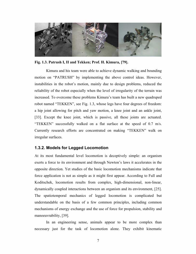
Fig. 1.3. Patrush I, II and Tekken; Prof. H. Kimura, [79].

Kimura and his team were able to achieve dynamic walking and bounding

motion on “PATRUSH” by implementing the above control ideas. However,

instabilities in the robot’s motion, mainly due to design problems, reduced the

reliability of the robot especially when the level of irregularity of the terrain was

increased. To overcome these problems Kimura’s team has built a new quadruped

robot named “TEKKEN”, see Fig. 1.3, whose legs have four degrees of freedom:

a hip joint allowing for pitch and yaw motion, a knee joint and an ankle joint,

[33]. Except the knee joint, which is passive, all these joints are actuated.

“TEKKEN” successfully walked on a flat surface at the speed of 0.7 m/s.

Currently research efforts are concentrated on making “TEKKEN” walk on

irregular surfaces.

1.3.2. Models for Legged Locomotion

At its most fundamental level locomotion is deceptively simple: an organism

exerts a force to its environment and through Newton’s laws it accelerates in the

opposite direction. Yet studies of the basic locomotion mechanisms indicate that

force application is not as simple as it might first appear. According to Full and

Koditschek, locomotion results from complex, high-dimensional, non-linear,

dynamically coupled interactions between an organism and its environment, [25].

The spatiotemporal mechanics of legged locomotion is complicated but

understandable on the basis of a few common principles, including common

mechanisms of energy exchange and the use of force for propulsion, stability and

manoeuvrability, [39].

In an engineering sense, animals appear to be more complex than

necessary just for the task of locomotion alone. They exhibit kinematic

7

redundancy because they have more joint degrees of freedom than their six body

positions and orientations. Animals show actuator redundancy for locomotion

because often they have at least twice as many muscles as joint degrees of

freedom. Moreover, they show neuronal redundancy. However, this complexity

can be reduced by introducing archetypical models, which encode sufficiently the

task of locomotion in the sense that they approximate well the centre of mass of

running animals or humans.

Two of the most common patterns of locomotion are walking and running.

At first glance, the difference between walking and running would appear

obvious. In running all feet are in the air at some point in the gait cycle, whereas

in walking there is always one foot on the ground. This distinction is appropriate

for most animals, however there are cases when it fails. McMahon and Chen

observed that when humans run along a circular path, the aerial phase of the

motion disappears if the turn has a sufficiently small radius, [47]. A better

criterion for distinguishing walking and running is that in walking the centre of

mass is at its highest point at midstance, while in running is at its lowest point.

Two basic mechanisms have been proposed to explain the different

patterns of time varying forces measured during walking and running, [22], [25].

In walking, the center of mass vaults over a rigid leg, analogous to an inverted

pendulum, see Fig. 1.4. At midstance the center of mass reaches its highest point.

Like a pendulum, the kinetic and gravitational potential energies of the body are

exchanged cyclically. Kinetic energy in the first half of the stance phase is

transformed into gravitational potential energy, which is recovered as the body

falls forward and downward in the second half of the stance phase. Blickhan and

Full showed the model to be general and not restricted to systems with upright

postures, when they discovered that eight-legged crabs employ four distributed

pendulums, which operate as one, [12]. As noted by Alexander [3], walking is

restricted to speeds somewhat less than gl , where g is the gravitational

acceleration and l is the leg length. Centrifugal effect on the walking trajectory

lightens the contact force at the foot; as the speed approaches gl , the total force

8

goes to zero. Breaking the “ gl ” barrier calls for a different type of gait, namely

running.

Fig. 1.4. Models for walking and running in the sagittal and horizontal plane:

Inverted pendulum (IP), Spring Loaded Inverted Pendulum (SLIP) and

Lateral Leg Spring (LLS).

In running, the leg acts as a spring compressing during the breaking phase

and decompressing during the propulsive phase. Diverse species that differ in

skeletal type, leg number and posture run in a stable manner like the Spring

Loaded Inverted Pendulum (SLIP) system, [3], [11], [12], [24], [47], [72] see Fig.

1.4. Like the SLIP, the kinetic and gravitational potential energies are stored as

elastic energy in the spring at the breaking phase and recovered in the propulsive

phase. In running, higher speeds can be achieved because the compression of the

spring diminishes the centrifugal effect, so that the leg remains in contact with the

ground through midstance. Raibert used the SLIP model to derive controllers that

managed the total energy of the centre of mass, to stabilise his legged robots.

Moreover, the virtual leg spring of insects consists of a tripod of legs on the

ground working as if they were one leg of a biped or two legs of a quadruped.

Therefore, it is natural to inquire whether or not the SLIP is just a descriptive

model or represents a model that advances hypotheses concerning the high-level

control strategy underlying the achievement of the task. An analytical in-depth

study of the SLIP can be found in [70].

9

Schmitt and Holmes, motivated by experimental studies of insects,

proposed a model similar with the SLIP to describe the motions of the body on the

horizontal plane, called the Lateral Leg Spring (LLS), [68]. In view of the typical

splayed insect posture, the LLS is a three-degree-of-freedom model analogous to

the SLIP, but with the spring compressed along a leg placed laterally in the

horizontal plane as shown in Fig. 1.4. It describes the behaviour of one or more

legs as the body bounces form side to side under the assumption that at “normal”

steady state motions, sagittal and horizontal plane dynamics might be only weekly

coupled, so that independent analysis could help towards understanding the full

six degrees of freedom motion.

In an attempt to set the basis for a systematic approach in studying legged

locomotion, Full and Koditschek introduced the concepts of templates and

anchors, [25]. A template is a formal reductive model that (a) describes and

predicts the behaviour of the body with respect to a minimum number of variables

and parameters and (b) advances hypotheses concerning the high-level control

strategy underlying the achievement of the task. An anchor is a more elaborate

dynamical system representing a more realistic model grounded in the

morphology and physiology of an animal. Anchors can reveal the mechanisms by

which legs, joints and actuators function to produce the behaviour of the template.

Therefore, an anchor is not only a more complex system but also must have

embedded the behaviour of its template. The anchor’s lower-level control action

coordinates the ankle, knee, hip joints and multiple legs to produce the motion of

the centre of mass of the torso according to the template. The higher-level control

action regulates the task-level behaviour such as the forward speed or hopping

height of the template. According to these definitions the inverted pendulum and

the spring loaded inverted pendulum presented above are templates for studying

walking and running in animals of various postures and leg numbers. To create a

template, redundancies in locomotion can be resolved by seeking for synergies

and symmetries.

Note that up to this point there has not been proposed in the literature a

template for studying sagittal plane motions in which the pitching oscillation of

10

the torso is one of the dominant modes. Indeed, none of the templates described

above captures the pitching motions, which are present in any real system. This is

one of the reasons for introducing a new template for studying the bounding and

pronking gaits where torso pitching is a dominant factor determining the stability

of the system.

1.3.3. Dynamic Stability Analysis

As was mentioned above, legged systems exhibit intermittent and highly

nonlinear dynamics. As a result, the equations of motion for a legged robot are a

function of the legs on the ground, and thus very different dynamics apply at

different phases of the gait. Each of the phases that constitute the cyclic motion

may be unstable, however the whole motion is stable. The mathematical

foundations of determining the dynamic stability of a running legged robot are

based on methods drawn from nonlinear dynamical system’s theory. For a

comprehensive introduction to discrete dynamical systems see [30]; more

advanced texts are [28], [37].

An important conceptual tool for understanding the stability of periodic

orbits is the Poincaré map, [28], [31], [37]. It replaces an nth order continuous-

time autonomous system by an (n-1)th order discrete-time system. The problem of

studying the stability properties of a periodic solution of a continuous-time system

is thus reduced to the problem of studying the stability of the periodic points of

the Poincaré map. In the context of dynamically stable legged systems one can

also find the terms stride function, [43], or return map, [35]. In order to define the

return map for a legged system a reference point in the cyclic motion must be

selected and then the dynamic equations must be integrated starting from that

point until the next cycle. It should be mentioned here that integrating the

equations of motion for a legged robot is not a trivial step (as for most real

systems). Analytical integration of the dynamics is usually not possible, except for

very simple cases. On the other hand, using numerical methods inevitably leads to

loss of insight, which is extremely important for identifying which parameters

affect the motion of the system. In trying to cope with that problem, many authors

11

use simple mathematical models of the robot, which capture the basic properties

that are dominant in the behaviour of the system, e.g. [17], [35], or they use

perturbation techniques to analytically approximate a solution, e.g. [7], [45].

Koditschek and Buehler were the first to derive and use a return map to

study the basic properties of Raibert’s vertical hopper, [35]. Their analysis relies

on exact integration of the dynamics to produce a return map that exhibits the

robot’s state at the next hop as a function of that at a previous. The authors

derived two simple models using linear and nonlinear springs that admit analytical

solutions. They assumed that the dominant force during the stance phase is the

spring force while they neglected gravitational and damping forces and

considered a zero thrust time. Their main result was that, using the nonlinear

spring model, improper choice of the controller parameters e.g. high thrust value,

may lead to stable steady-state behaviour characterised by repeated long-high-hop

(period 2 point), short-low-hop alternations, a case that was reported by Raibert as

limping gait. With respect to the linear spring model, the authors concluded that

over the range of physical valid parameters the strongly stable equilibrium

behaviour persists.

Vakakis and Burdick extended the analysis in [35], by deriving a more

complete model of the one-dimensional hopping robot, [80]. Their model relaxes

the assumption of instantaneous thrust time. They showed that the return map

derived in by Koditschek and Buehler [35] based on the assumption of zero thrust

duration is structurally unstable i.e. it exhibits the classic period doubling route to

chaos and the existence of a strange attractor. They concluded that when the thrust

time is sufficiently large, the strange attractor collapses and the robot exhibits

globally stable uniform hopping motion for a large range of model parameters.

Ostrowski and Burdick considered the design of feedback algorithms for

controlling the periodic motions of the one-dimensional hopping monopod, [53].

Their paper suggests a parameter (e.g. thrust, thrust duration, leg stiffness)

feedback law to shape the return map in a neighbourhood of a fixed point. The

proposed algorithm “flattens” the return map around the fixed point causing a

wide range of initial conditions to quickly converge to the fixed point, while at the

12

same time the region of the desirable period-1 behaviour is significantly enlarged.

The authors use an interesting technique to derive the Poincaré map based on

computing system energy before and after a non-conservative phase, thus

avoiding the need to integrate the equations of motion.

M’Closkey et al. presented a more complicated two-dimensional monopod

model, which included both forward and vertical hopping dynamics, [46]. Based

on the same assumption as in the previous papers, they extended the 1-DOF

model to a 2-DOF model that includes forward motion. The authors used

Raibert’s foot placement algorithm (FPA). Note that the FPA does not enter

explicitly into the dynamic equations because the leg is assumed massless,

however it determines the initial conditions for the ensuing phases. The authors

derived an analytical approximation of the return map using perturbation methods

under the assumption of low speeds and then they checked the validity of their

perturbation solution by comparing it with an exact numerical solution based on

the system’s integrals of motion. Among their main findings is that the period

doubling bifurcation persists in the 2-DOF system and it is an effect of the

nonlinear spring: Using a linear spring resulted in no bifurcations.

In a more recent paper, Schwind and Koditschek study a completely

passive monopod where the only control exerted is the placement of the leg at

touchdown, [69]. The authors derive an analytical expression of the return map

based on the common assumption of negligible gravitational force during stance.

They formally proved that the existence of a periodic motion requires for the

stance phase to be symmetric. The stability analysis of the fixed points under

Raibert’s simple decoupled feedback velocity control law showed that it yields

good regulation, however better regulation can be achieved by using coupled

feedback that takes the dynamics into account. They also discovered that both the

set of the fixed points and its domain of attraction grow as the spring constant is

increased.

The intermittent and highly nonlinear nature of the differential equations

that govern the motion of locomotion systems severely limits the usefulness of the

discrete dynamical system theory in analysing the behaviour of these systems. To

13

compensate for this, Li and He presented an alternative approach for the analysis

of a one-legged hopping robot, called the energy-balance method, [38]. The

authors consider that the hopper consists of three components: a conservative

(Hamiltonian) component, a dissipative component and an actuator component.

The dissipative and energy-generating components are viewed as perturbations to

the Hamiltonian system, whose analysis is much easier since it admits an

analytical solution. The fixed points are then calculated by considering that the

energy change along a limit cycle has to be zero i.e. the energy generated has to

balance the energy dissipated along a limit cycle. This is equivalent to the fixed

points of the Poincaré map. Moreover, the authors state a criterion for the stability

of the limit cycle. These conclusions are then used to study the existence and

stability of the limit cycles of the one-dimensional hopper.

All the above results concern monopods that were studied initially by

taking into account only the vertical hopping motion but then expanding the

model to include also the forward motion. There are not many results in deriving

and analysing return maps for quadrupedal running gaits. The only results are due

to Berkemeier, [7], [8], [9]. Berkemeier considers a 2-DOF model for quadrupedal

running in place and he studies the bounding and pronking gaits of four-legged

animals. Approximate return maps are constructed around both trajectories, and

these are used then to derive explicit expressions for the amplitude and stability of

the gaits. Berkemeier considered massless legs and small pitch angles to derive a

linear model. Note that even using a linear model, which, as is well known, can be

integrated analytically, it is not possible to derive an analytical expression for the

return map! This is because the equations that result from integrating the model

cannot be inverted to solve for the lift-off time, so perturbation expansions in

damping and thrust length were used. The above results suggest that simple, local

energy-pumping feedback is sufficient to produce stable bounding and pronk.

Moreover, the author found that pronking produces more ground clearance than

bounding for the same effort, but it becomes unstable for larger hopping heights.

14

1.3.4. Passive Dynamics

With the term passive dynamics we mean the unforced response of a system under

a set of initial conditions. In general, characterising the properties and conditions

of the passive behaviour and identifying regions of the model parameters where

the system can passively stabilise itself, can lead to designing controllers, which

are not entirely based on continuous state-feedback like computed-torque

controllers. Control strategies should work with the natural dynamics rather than

cancel them out! Raibert and Hodgins stated, “We believe that the mechanical

system has a mind of its own, governed by the physical structure and laws of

physics. Rather than issuing commands, the nervous system can only make

suggestions, which are reconciled with the physics of the system and task [at

hand]”, [64].

To explore the role of the mechanical system under control, Kubow and

Full developed a simple two-dimensional dynamic model of a hexapedal runner

(death-head cockroach, Blaberous discoidalis), [36]. The authors decided to

model sprawled posture arthropods because of their stability, simple nervous

system and the increased probability that their mechanical system contributes to

control. Since sprawled posture animals operate mostly in the horizontal plane,

the authors decoupled the model from the sagittal plane and only modeled the

horizontal plane. The model had no equivalent of nervous feedback among any of

its components and it was found to be stable at velocities, which are similar to

those measured in the insect at its preferable velocity. Surprisingly, Kubow and

Full discovered that the model self-stabilised to velocity perturbations.

Perturbations altered the translation and/or rotation of the body, which provided

mechanical feedback by changing the moments generated during the motion.

Recovery from perturbations depended on the type of the perturbations (fore-aft

velocity, lateral velocity and rotational velocity perturbations). This work first

revealed the potential importance of mechanical feedback in simplifying neural

control by demonstrating that stability could result from leg moment arm changes

alone.

15

This self-stabilised behaviour of the mechanical system without the need

of any feedback mechanism analogous to the nervous system, was formally

proved by Schmitt and Holmes in the context of the Lateral Leg Spring (LLS)

template, described in Section 1.3.2, see Fig. 1.4, [68]. Although inertial effects

are important in rapid running and control and stabilisation might be thought of as

a complex task requiring sophisticated neural feedback, Schmitt and Holmes

showed that such feedback is unnecessary. The primary task of the neural Central

Pattern Generator (CPG) in fast running is to “set the pace” and determine long-

term control objectives such as the heading and speed, leaving body mechanics to

take care of stability in the short term.

The fact that even without any modeled energy dissipation, the LLS

template can exhibit stable periodic motions that remove the need for continuous

or intermittent feedback in correcting responses to perturbations, motivated

Chigliazza et al. [17] and Seyfarth et al. [72], to study how the SLIP template

responds to departures from the conditions of cyclic motions. Seyfarth et al.,

based on computer simulations, found that for certain touchdown angles, the SLIP

becomes self-stabilised if the leg stiffness is properly adjusted and a minimum

running speed is exceeded. At a given speed, stable running is characterised by an

almost constant maximum leg force. They discovered that by increasing speed,

the system becomes less sensitive to perturbations, i.e. larger variations in leg

stiffness and touchdown angles are tolerated by the system. Independent work

conducted by Chigliazza et al. demonstrated and, under simplifying assumptions,

rigorously proved that asymptotically stable periodic gaits for the SLIP model

exist over a range of parameter values. The authors, based on the common

assumption that the gravitational force can be considered negligible during the

stance phase, derived analytically a Poincaré map and performed detailed

bifurcation and parameter studies. They also discussed the limits of passive

stability and they provided some explanations of the mechanisms, which might be

responsible for that self-stabilised behaviour. Note that stable periodic gaits for

the SLIP have appeared in the literature before Seyfarth’s and Chigliazza’s

contributions, see Altendorfer et al. in [5].

16

In the context of quadrupedal robots Murphy discovered that the

distribution of mass between the hips in the body has a profound influence on the

behaviour of a running system, [51], [52]. He studied the bounding and pronking

gaits of a quadruped robot using a model that includes leg inertias while the leg

length is completely controllable using linear actuators. He defined a

dimensionless group that represents the normalised moment of inertia of the body

called dimensionless moment of inertia, j = I / mL2 where I is the moment of

inertia of the body, m is the mass of the body and is half the hip spacing.

Murphy found that when the attitude of the body can be passively stabilised

in a bounding gait. When stabilisation is not so easily obtained and active

control has to be employed. His model had actuators, thus it was not a passive

conservative system. However, the reference to his work is placed here under the

Passive Dynamics survey, because the dimensionless moment of inertia, which

described how the mass is distributed between the hips, has a profound effect in

the system’s natural motion.

L

j <1

j >1

A rigorous proof of Murphy’s conclusions can be found in Berkemeier,

[9]. Linearization of the bounding return map showed that bounding is unstable

for a dimensionless moment of inertia greater than one, while local analysis was

inconclusive for the case where the dimensionless moment of inertia is lower than

one. However, simulations showed stable bounding motion when the

dimensionless moment of inertia is lower than one, a fact that agrees with

Murphy’s conclusions in [51], [52]. In the case of pronking, local stability

analysis of the return map showed a rather complicated dependence on inertia and

height.

Brown investigated the conditions for obtaining passive cyclic motion,

[13]. The author studied two limiting cases of system behaviour: The grounded

regime, where the feet do not leave the ground and the flight regime, where stance

periods are considered to be infinitesimally short. Brown found that the system in

either regimes can passively trot, gallop or bound if provided with the proper

initial conditions. However, this behaviour can occur only if the properties of the

system – mass m , moment of inertia I and half-hip spacing – have a particular L

17

relationship, . This differs from the findings of Murphy in [51], [52],

because Brown considers conditions for repetitive cyclic motion while Murphy

sought conditions for passive stability of a nonconservative system. It must be

mentioned here that the above analysis was performed for each of the two regimes

independently. However, in quadrupedal running gaits like bounding, both

regimes participate in constituting the cyclic motion. As will be seen in Chapters

3 and 4, passively generated cyclic motions exist and in addition, there are ranges

in system parameters where the system is passively stable.

I / mr2 =1

Simulations and analysis suggest that suitably designed legged machines

will be able to run passively i.e. without actuation and control. However, due to

practical limitations (energy losses are inevitable) there are no legged robots

which operate completely passively, except McGeer’s passive dynamic walkers

[44]. McGeer built a gravity powered biped for which walking is a natural mode.

When the robot starts on a shallow slope, so as to compensate for the energy

losses due to inelastic impacts, it converges to a steady gait, which is similar to

human walking, without active control or energy input. McGeer performed an

analysis of the mechanics of the steady walking cycle and studied its stability by

constructing a step-to-step function, analogous to the return map developed in the

study of the SLIP dynamics or the LLS templates. The response of the system to

large perturbations and the effect of parameter variations in the generation of

passively generated and stabilised walking gaits were also studied. Experiments

with a test machine verified that the passive walking effect could be readily

exploited in practice. McGeer expanded his analysis to passive bipedal running in

[43], although he did not provide any experimental results on that. Garcia et al.

following McGeer’s work studied the simplest possible two-dimensional passive

biped, [26]. Their model exhibits self-stabilised behaviour just as McGeer’s more

complicated model. Analytical calculations found initial conditions and stability

estimates for period-one limit cycles. They found that increasing the slope, stable

cycles of higher order appear and finally the walking-like motions become chaotic

through a sequence of period doubling. Smith and Berkemeier extended McGeer’s

work from bipedal to quadrupedal locomotion by first analysing a rimless wheel

18

and then a more complex model of a quadruped with stiff legs, where they found

that quadrupedal walking is unstable, [74].

1.4. Previous Work in ARL

The Ambulatory Robotics Laboratory (ARL) at McGill University was founded

by Professor Martin Buehler in 1991. Motivated by Raibert’s work, Buehler and

his students developed dynamically stable running robots. ARL robots exhibit low

degree of freedom electrical actuation coupled with a minimalistic approach to

mechanical complexity. Radialy compliant leg designs, which decouple the

actuators from gravitational loads, are used. The complete system features

dynamic mobility and autonomy2. The controller design of our robots shares a

reliance on the passive dynamics of their suitable designed dynamical system,

minimal reliance on complex state-feedback based controllers and increasingly

biological inspiration. It is believed that these fundamental design and control

principles are crucial for the success of any legged machine, measured in terms of

stability, energy efficiency and speed. For a survey of the research in dynamically

stable legged locomotion in the ARL the interested reader is referred to [14].

The first dynamically stable robot that was built in ARL was the Monopod

I, [1], [2], see Fig. 1.5. It consisted of a body connected to a compliant prismatic

leg at the hip joint and it was constrained to move in the sagittal plane via a

planariser. Monopod I demonstrated that designing the dynamical system by

taking into consideration right from the beginning the compliance, the actuator

and transmission system and the operating modes, it was possible to achieve

dynamically stable locomotion with reduced actuator power and energy densities.

Monopod I was able to run at a speed equal to 1.2 m/s with an average mechanical

power of 125 W. The control algorithms for the pitch and forward speed used

were based on Raibert’s decoupled controllers for forward speed, hopping height 2 There are multiple definitions of autonomy. Usually it is used to identify that a machine is

capable of some (limited) decision-making processes. However, in this thesis the word autonomy

is used to identify that the system has all the power and computation it needs on board for

untethered operation.

19

and body pitch. Moreover, a thrusting controller based on the model of the

transmission system was proposed to transfer sufficient energy during the short

stance phase, [27].

Fig. 1.5. Monopod II (left), and Scout I (right).

Aimed for lower consumption, Monopod II was built in the mid 1990s,

and inherited most of the features of Monopod I. Energetic analysis of the

experimental results showed that at top speed, 40% of the energy goes to

sweeping the leg forward, [27]. To reduce this energy, series compliance in the

hip was introduced resulting to a properly sustained body-leg counter oscillation.

A robust controller for that system was proposed in [2]. The controller is using the

robot’s passive dynamics to determine desired hip joint trajectories for any given

forward speed. In addition, minimal actuation is used to compensate for the

energy losses and system stabilisation. Hopping height was controlled via a new

adaptive energy-based feedback controller. Implementation of this control

strategy, also known as Controlled Passive Dynamic Running (CPDR), improved

the energy efficiency by factor of two! Monopod II achieved stable running at a

speed equal to 1.2 m/s with total mechanical power expenditure at 48%.

Motivated by the feasibility of dynamically stable robots with fewer

actuators than degrees of freedom, which move fast and efficiently based on

standard electric motors, such as the ARL Monopods I and II, and to further study

the mechanical simplicity in legged systems, Scout I was designed and built, [15],

20

[16], see Fig. 1.5. With stiff legs and only one actuator per leg located at the hip

joint, this prototype exhibited a wide variety of behaviours such as walking,

sidestepping, turning and step climbing up to 45% of leg length, [83]. The robot

walks by rocking back and forth by keeping the front legs stationary while the

back legs touch down and sweep backwards. The proposed controller required

minimal actuation and sensing and the significant facts on the

Extending the single-actuator-per-leg design idea that enabled Scout I to

walk dynamically, Buehler and his team designed the Scout II quadruped, [6],

[16], [18], see Fig. 1.6. Scout II has been designed for completely autonomous

operation, with the actuators, batteries and computing equipment contained in the

robot’s body. Its mechanical design is an exercise of simplicity. Each leg

assembly consists of a lower and an upper leg connected via a spring to form a

compliant prismatic joint. Therefore, each leg has two degrees of freedom, one

actuated at the hip and one radial, which is not actuated. Scout II is an

underactuated, highly nonlinear intermittent dynamical system with multiple

constraints. Despite this complexity, simple control laws can excite the robot’s

dynamics and can stabilise periodic motion that result in robust and fast running,

without requiring task level feedback, [54], [55], [57], [77], [78].

The control action is based on two individual independent leg controllers,

without a notion of the body state, refer to [55], [57], [78]. During flight, the

controller servos the leg at a desired touchdown hip angle and then, during stance,

it sweeps the leg hip backwards with constant commanded torque until a sweep

limit angle is reached. The resulting bounding motion is due to the interaction of

the controller with the dynamics of the system. Variations of the above controller

resulted in the same robust and natural bounding motion at top speeds between

0.9 and 1.2 m/s, [57], [77], [78]. Note that similar controllers have been recently

implemented on the SONY AIBO dog to make it bound, [82]. Apart from the

bounding running gait, Scout II legs were modified so as to implement the trotting

gait, in which diagonal legs work in pair, [29]. In doing so, the leg design has

been modified and a completely passive knee, which relies on the natural

dynamics and the dynamic coupling with the upper leg, was designed and added

21

to the robot, see Fig. 1.6. Scout II exhibits various other behaviours such as

dynamic compliant walking, see [20], [21] and step climbing, see [77].

Fig. 1.6. Scout II with compliant legs (left) and lockable passive knees (right).

Motivation from recent research in biology and biomechanics, [23], lead

to the design and construction of RHex, [67], a hexapedal robot that captures

some of the biomimetic functions of running cockroaches, [5], Fig. 1.7.

Fig. 1.7. RHex in rough terrain and on stairs.

As in Scout II the RHex’s body contains all the necessary actuators,

batteries, computational power, I/O and sensing. Each leg has again one actuated

degree of freedom located at the hip while the radial degree of freedom is

compliant, unlike most of the other hexapods built to date. RHex walks with a

compliant tripod gait, and eliminates toe clearance problems by rotating the legs

in a full circle. The tripod gait with its four parameters described above enables

RHex to transverse a large variety of obstacles and move over rugged and highly

fractured terrain at speeds of one body length per second. The pronking gait is the

first dynamically stable gait implemented on the robot, [48]. To date, RHex has

22

demonstrated one of the key advantages of legged robots over wheeled platforms:

versatility.

1.5. Thesis Contributions and Organisation

In this thesis, in an attempt to understand why simple control laws result in robust

high performance running, [55], [57], [78], we explore the potential role of the

mechanical system of the robot in the generation and control of the running

bounding gait. Increasing evidence from analysis and experiments in biology and

biomechanics suggests that at intermediate and fast speeds in locomotion tasks,

the dynamics of the mechanical systems dominates the motion. In a sense, control

algorithms are embedded in the morphology itself. The author’s contributions to

identifying similar behaviours in Scout II include the introduction and analysis of

a simple model i.e. a template to study the passive dynamics of the robot in the

bounding gait. More specifically:

• A template for studying quadrupedal gaits with pitching is introduced and its

equations are developed. The related literature lacks such a template for

studying running gaits where the pitch oscillation significantly affects the

stability of the system.

• A numerical method is developed to identify passively generated cyclic

motions for the template introduced. Symmetry conditions for achieving

passive bounding are discovered.

• A regime where the system can be self-stabilised against perturbations is also

found. It was discovered that self-stabilisation behaviour is achieved in higher

forward speeds, a fact that is in agreement with recent research in biology and

biomechanics.

• Comparison between the stability of pronking and bounding is performed,

which explains why the robot “prefers” bounding than pronking in higher

speeds.

• The self-stabilisation property in the SLIP is revised. This result will help in

avoiding confusions with the fact that flatter touchdown angles are needed to

accommodate larger speeds.

23

The structure of the thesis is as follows. In Chapter 2, the basic

terminology of legged locomotion is introduced. Terms like step, stride, gait,

virtual leg are defined and the most common quadrupedal gaits are described.

Scout II is introduced and the basic assumptions for modeling its dynamics in the

bounding running gait are justified. The equations that govern the motion of the

system are presented and some comments on the transition conditions are given.

Finally, the motor driving system and the transmission system, which are essential

not only for constructing more accurate simulations but also for understanding the

robot’s behaviour, are modeled. In Chapter 3, the tools for studying the passive

dynamic behaviour of Scout II are introduced and the self-stabilised behaviour in

the SLIP is briefly described and revised. A return map describing the bounding

running gait is numerically constructed and a searching procedure for finding

passively generated cyclic motions is proposed and discussed. This method for

locating fixed points of the return map is improved and a more systematic

procedure for finding fixed points is proposed in Chapter 4. This is done based on

some of the symmetric properties of the cyclic motions found. Local stability

analysis of the fixed points is performed resulting to the very important

conclusion that there exists a regime where the system tolerates departures from

cyclic motion without any control action. This self-stabilised property of the

model improves as the forward speed increases and hopping height decreases, a

result which is in agreement with the findings in biology and biomechanics. The

thesis ends with conclusions and future recommendations in Chapter 5.

24

Chapter 2

Scout II Bounding Models for Analysis and Simulation

2.1. Introduction

In this chapter, the equations that govern the motion of Scout II are developed

using the Lagrangian methodology. These equations are essential for analysing

the behaviour of Scout II, and they will be used in the next chapter to draw

valuable conclusions on characterizing the natural dynamics of the robot. In

deriving the equations of motion for Scout II in the bounding gait we assume that

the mass and the moment of inertia of the legs are negligible with respect to the

inertia properties of the body. This assumption simplifies the equations so as they

are mathematically tractable and they could be used for analysis, while at the

same time they capture the basic properties of the behaviour of the robot.

The structure of this chapter is as follows: In Section 2.2, the most

common quadruped running gaits are briefly described and a two-dimensional

model for Scout II, which describes the dynamics of running in the sagittal plane,

is introduced. Before proceeding with deriving the equations of motion for the

above model, the Lagrangian formulation is recalled and the basic assumptions

used are discussed in Section 2.3. In Section 2.4, the equations of motion for the

Spring Loaded Inverted Pendulum (SLIP) model are derived. In Section 2.5, the

equations of motion for Scout II following the bounding gait are developed using

both Cartesian and joint variables. In the same section the transition equations

describing the events that trigger the phases of the bounding motion are given

25

along with some comments concerning the numerical integration of the

differential equations of the models. In Section 2.6 simple mathematical models

for the battery and the motor driving system, which are essential for constructing

accurate simulations of the robot, are developed. The chapter ends with describing

a more accurate model developed in Working Model, which is a replica of the

physical system. These, more accurate simulations, are used to test controllers

before implementing them on the real robot rather than analysing them.

2.2. Running Gaits and Locomotion Models

In this section, we briefly describe the basic quadrupedal running gaits and we

introduce a model, which will be used to analyse the basic qualitative properties

of quadrupedal running in the sagittal plane. By taking into account synergies and

symmetries, the complexity of two-, four- or six-legged animals and robots can be

reduced to relatively simple models, which can then be used to analyse the

system’s behaviour, [25]. By synergies, we mean parts that work together in

combined action or operation e.g. groups of muscles, joints, legs etc. By

symmetries we mean the correspondence of parts on opposite sides of a plane

through the body. The equations of motion for the models introduced here will be

derived in subsequent sections.

When an animal is moving forward, its legs have a progressive and

retrogressive motion with respect to the body. Animal locomotion typically

employs several distinct leg movements, known as gaits. Most gaits can be

represented as symmetrical, cyclical patterns of leg movements, [19]. By

convention, one gait cycle spans the interval from footstrike of some reference

foot to consecutive footstrike by the same foot. During the motion, each leg is

either in contact with the ground i.e. in stance or in the air i.e. in flight3.

According to Muybridge, a step is an act of progressive motion, in which one of

the legs is lifted from the ground, thrust in the direction of the movement and

3 Note that sometimes when all the legs are in flight we call the entire robot or animal to be in

flight. Otherwise the robot or animal is called to be in stance.

26

placed again on the ground, [49]. A stride is a combination of actions, which

requires each one of the legs to be –either alone or in association with another leg-

lifted from the ground in its regular sequence, thrust in the direction of the

movement, placed again on the ground and repeat its motion, [49].

The duty factor of the foot is the fraction of the gait cycle for which it is in

contact with the ground. At a first glance, the difference between walking and

running would appear obvious. Running gaits usually have duty factors less than

0.5; thus there are periods in running when all the legs are in the air, called

ballistic or flight phases. Walking gaits have a duty factor more than 0.5; thus

there are periods when all the legs are simultaneously on the ground, [19].

However, as McMahon and Chen point out, this distinction between walking and

running is incomplete since it may hold most of the time for most animals, but

there are times when it fails, [47]. A better criterion for distinguishing would be

that in walking the centre of mass is highest in mid-step, while in running it falls

at its minimum height, [47].

Concerning stability, gaits can be divided in statically stable or

dynamically stable, [62]. A statically stable system follows gait patterns where the

body and legs move in such way to keep the centre of mass within the polygon

formed by the legs that are in contact with the ground. Unlike statically stable

robots, a legged system that balances actively can tolerate departures of the center

of mass from the support polygon formed by the legs in contact with the ground.

The realization of dynamic gaits results in smoother and more natural motions,

higher mobility and higher speeds than those achieved in static gaits, while at the

same time it requires less power.

The most common quadruped running gaits are the bound, the pronk, the

trot, the pace and the gallop, the last of which usually appears in two variations:

rotary gallop and transverse gallop. Fig. 2.1 shows gait diagrams presenting the

pattern of leg use in all the gaits described above. Detailed descriptions of the

running gaits have been available since the 19th century; see Muybridge [49]. All

the above gaits, except the gallop, are simple in that the legs are used in pairs. In

trotting, the legs work in diagonal pairs: the left front and the right back (LF-RB),

27

strike the ground at the same time and they swing backwards in phase. Bounding

uses the front legs in pair (LF-RF) and the back legs in pair (LB-RB) while pacing

uses the lateral legs in pairs (LF-LB and RF-RB). In pronking, all the legs are in

phase: they all strike and leave the ground at the same moment. Galloping is a

more complicated gait, which resembles the bounding gait with the difference that

the legs forming the front and back pairs are slightly out of phase resulting in a

motion that is not confined to the sagittal plane.

LFLB

RB

RF

LFLB

RB

RF

Symmetric Bounding

Pacing

Trotting

Pronking

Rotary Galloping

Transverse Galloping

LFLB

RB

RF

LFLB

RB

RF

LFLB

RB

RF

Running Cycle

LFLB

RB

RF

LF RF

L B R B

Fig. 2.1. Gait diagrams showing the pattern of leg use in different running

gaits. Shaded areas represent legs that are on the ground while blank areas

represent legs that are in the air. Indexes: L for Left, R for Right, F for Front

and B for Back.

In this thesis, we restrict our attention to the bounding running gait rather

than pronking. As can be seen from Fig. 2.1 the essentials of the motion in

bounding takes place in the sagittal plane. Thus in bounding the motion is

assumed planar. In planar motion, Scout II can be considered as a three-body

chain composed of the torso and the front and back leg pairs, also called the

virtual legs, see Fig. 2.2. The notion of virtual legs has been used with great

success by Raibert to control his two- and four-legged robots by extending the

one-leg control algorithms, [60], [63]. It allows several separate physical legs to

be represented by fewer virtual legs, Fig. 2.2. For instance, the front and back

28

virtual legs represent the pair of the front and back physical legs of the robot. The

virtual legs and the original pair of physical legs both exert the same forces and

moments on the robot’s body so they both result in the same behaviour.

According to Raibert, [63], for the assumption of the virtual legs to be valid the

following conditions have to be true for the bounding gait:

• The torque delivered at the hips of the physical legs should be equal to half the

torque delivered at the hip of the virtual leg.

• The axial force exerted by the springs of each of the physical legs has to be

half the force exerted by the spring of the corresponding virtual leg.

• The feet of the physical legs forming a virtual leg should strike the ground in

unison and leave the ground in unison.

• The forward position of the feet of the virtual leg with respect to the hip has to

be the same with the forward position of the feet of the physical legs.

Sagittal Plane

FrontVirtual Leg

BackVirtualLeg

Physical Legs

Fig. 2.2. The concept of virtual legs for the bounding gait.

To derive the equations that describe the dynamic behaviour of Scout II

the two-dimensional model presented in Fig. 2.3 is used. The legs are connected

to the body through revolute joints, which are driven by rotary actuators. Each leg

includes upper and lower sections, which are connected with a linear spring. The

distance between the toe and hip changes because of the sliding motion between

the lower and the upper section of the legs, so each leg has one linear passive

degree of freedom. The energy dissipation resulting from the contact between the

upper and the lower part of the leg, taking place via a viscous fluid i.e. a lubricant,

29

is modeled using a damper in parallel with the spring. To summarise, each leg has

two degrees of freedom: a rotational one, which is controlled via an actuator, and

a linear one, which is completely passive.

Torso

Toe

Lower Leg

UpperLeg

HipJoint

Back Leg

Front Leg

Spring &damper

Fig. 2.3. The two-dimensional model for Scout II in the sagittal plane.

In a complete bounding cycle, a full stride of the robot can be divided in

four different phases, see Fig. 2.4. These phases are:

• Back Leg Stance: In this phase, the back legs support the robot while the front

legs are in the air.

• Double Leg Stance: In this phase both legs are on the ground.

• Front Leg Stance: In this phase, the front legs support the robot while the back

legs are in the air.

• Double Leg Flight: In this phase both legs are in the air.

Each of the above phases is triggered by an appropriate event: touchdown or lift-

off. These events occur for each of the front and back legs so four events can be

defined: back leg touchdown, front leg touchdown, back leg lift-off and front leg

lift-off. As can be seen from Fig. 2.4 each of these events initiates the

corresponding phase. It must be mentioned here that the bounding gait under

study differs from the one presented in Fig. 2.1 by the absence of a flight phase

after the back leg stance. This reflects the physical reality of our robot’s passive

dynamics. Indeed, after the back leg stance the robot proceeds with a double

stance phase followed by a front leg stance while in the bounding gait presented

in Fig. 2.1 after the back leg stance phase the robot would have proceeded with a

30

double leg flight followed by a front leg stance. Note that, whether the robot will

converge to one or the other bounding cycle depends on its physical properties,

i.e. leg stiffness, total mass and mass distribution between the hips, which

determine the stance duration for each leg and on the control action.

BACK LEG STANCE DOUBLE LEG STANCE

FRONT LEG STANCEDOUBLE LEG FLIGHT

front leg touchdown

front leg lift-off

backleg

lift-offba

ckle

gto

uchd

own

Fig. 2.4. Snapshots of the robot at different phases and events triggering each

phase.

During bounding running each of the phases that compose the cyclic

motion of the robot is characterized by different sets of constraints among the

variables chosen to describe the system. Thus, the equations that describe each of

the phases are different, a fact that places Scout II in the category of intermittent

dynamical systems, also called variable structure systems. It will be apparent that

this feature, in combination with the highly nonlinear nature of the equations,

greatly complicates the analysis of Scout. In the following sections, the equations

are derived for each phase separately.

2.3. Notation and Assumptions

Before proceeding with deriving the equations that describe the dynamics of the

running motion, the Euler-Lagrange equations are recalled, [50], [71]. A

31

mechanical system with degrees of freedom is completely described by its

independent generalized coordinates, which are stored in the -dimensional

vector . If is the Lagrangian of the system calculated by subtracting the

potential energy V from the kinetic energy , i.e.

n n

n

q L

T

L T V− , (2.1)

the Euler-Lagrange equations are

d L Ldt

∂ ∂ ∂Π ∂− = −

∆∂ ∂ ∂ ∂ q q q q

, (2.2)

where is the power supplied to the system and Π ∆ is the Rayleigh dissipation

function, or for brevity the dissipation function of the system. In all the phases the

dynamic equations of Scout II can be written into the matrix form

( ) ( ) ( ) ( ) ( ), el+ + + + =uM q q V q q F q F q G q E q τ , (2.3)

where is the mass matrix, ( )M q ( ),V q q is a vector containing the velocity

dependent forces (centrifugal and Coriolis forces), is a diagonal matrix

containing the viscous friction coefficients,

uF

( )elF q is the vector of the spring

(elastic) forces, is the vector of the gravitational forces, is the

actuation distribution matrix and contains the actuation torques. In deriving the

equations of motion for Scout II in the form of Eq. (2.3) all the analytical

calculations were done in MATHEMATICA, [81].

( )G q ( )E q

τ

To derive a mathematical model for Scout II the following simplifying

hypotheses are taken into consideration:

• The mass and the moment of inertia of the legs are small in comparison with

the mass and the moment of inertia of the torso. Thus, massless legs will be

assumed.

• When a toe is in contact with the ground, it will be treated as a frictionless pin

joint. This implies that no slipping between the toe and the ground occurs and

that the toe makes point contact with the ground.

• Frictionless hip joints are assumed.

32

The first hypothesis greatly simplifies the equations by reducing the

dimension of the state space. Moreover, the evolution of the variables is

continuous and algebraic transition equations describing the impulsive impact

events resulting in step changes in generalised velocities are not necessary. Note

that this assumption may result in discrepancies mainly in the evolution of the

pitch angle θ of the robot. For instance, in the double leg flight phase there are no

external forces, which generate moments about the torso’s Centre of Mass

(COM), so the total angular momentum is conserved. As a result, any motion of

the legs results in changes to the torso pitch angle, which are not captured by the

proposed model. However, analysis showed that the error introduced in the pitch

angle during the flight phase is very small, [54]. It must be mentioned here that

the conservation of angular momentum during the flight phase results in a set of

constraints that are nonholonomic in nature, [50], allowing for some control

action to be taken, which would drive the pitch angle at a desired target value

before the next touchdown. However, model limitations such as the small mass of

the legs in comparison with the mass of the torso in combination with the

extremely small duration of the double flight phase exclude this possibility.

The second hypothesis simplifies the derivation of the equations of motion

since geometric constraints among the variables can be derived, which reduce the

number of the independent coordinates needed to completely describe the

configuration of the robot. In is true that during stance there may occur several

switches between forward-slipping, backward-slipping and no-slipping boundary

conditions. However, to ensure normal operation of the robot a slippage controller

has been implemented. This controller reduces the amount of hip torque applied at

the legs on stance based on a quasi-static model that predicts the maximum

friction force available. It is therefore safe to assume that the second hypothesis is

true. For details concerning the derivation and implementation of the slippage

controller refer to [54] and [77].

33

2.4. SLIP Dynamics

Before deriving the dynamic equations of Scout II in bounding motion, we study

the Spring Loaded Inverted Pendulum (SLIP) model, which, as was mentioned in

Section 1.3.2, is widely used for studying running in humans and animals. In this

section the equations of motion for SLIP, Fig. 2.5, are developed. As was

mentioned in Section 1.3.2, the SLIP provides a simple model that captures the

dominant properties of running in the sagittal plane, which do not depend on the

fine details of body structure.

m

0, k l

Neutral Point

nx 1nx +

tdγSymmetric Stance

Phase

nx 1nx +=

Fig. 2.5. Spring Loaded Inverted Pendulum (SLIP): A template for running.

Mechanical parameters and variables with sign conventions.

As Full and Koditschek note in [25], animals that differ in leg number,

posture and skeletal type run in the same manner, like a sagittal spring-mass

system, which is shown in Fig. 2.5. When humans run, their COM falls to its

minimum height at midstance, like a spring that compresses in the first half of the

step and decompresses in the second half recovering the elastic energy stored

during compression, [22]. Note that this fact is used to distinguish between

walking and running and is captured by SLIP, [47]. It must be mentioned here that

exactly the same COM motion is observed in dogs or even cockroaches when they

run: The virtual leg spring of six-legged insects consists of a tripod of legs on the

ground, where three legs work exactly as if they were one leg of a running biped

or two legs of a quadruped.

34

Experimental evidence suggests that the SLIP is not only a descriptive

simple model but it represents a true template for animal locomotion. Indeed, data

from experiments with humans on a treadmill showed very good match with

simulation data based on the SLIP model, [25], [47], [72]. Raibert also used the

SLIP as a template to derive control algorithms to stabilise his monopod and

based on these algorithms he managed to control two- and four-legged robots,

[62]. Note also that as was mentioned above, in pronking all the legs touch and

leave the ground in unison. Therefore, we can assume that the action of the four

legs is equivalent to the action of one virtual leg attached at the COM of the torso,

thus SLIP can also be used to describe Scout II in the pronking behaviour4.

Fig. 2.5 shows a stride of the SLIP model. Every stride can be divided into

a stance phase with the foothold fixed and the body moving forward while

compressing and decompressing the springy leg and a flight phase where the body

follows a ballistic trajectory under the influence of gravity. The dynamic

equations that govern the system’s behaviour are different due to the different

constraints that apply in the different phases. The parameters of the system and

the variables along with the sign conventions are presented in Fig. 2.5.

The equations of motion during flight are the ballistic COM translation of

the body, which may be integrated to give

( ) lo lox t x x= + t , (2.4a)

21( )2

lo loy t y y t gt= + − , (2.4b)

where x , denote the Cartesian coordinates of the COM with respect to a global

frame of reference and the superscript lo denotes the value of the variable at lift-

off.

y

During stance the toe is in contact with the ground and it will be treated as

a frictionless pin joint resulting to the following geometric constraints

4 It would be more accurate to replace the point mass in the SLIP with a body with specific values

of mass and moment of inertia, since such a model would include the pitching motion.

35

sintoex x l γ= − , (2.5a)

cosy l γ= , (2.5b)

where toex is the horizontal position of the toe.

Differentiating Eqs. (2.5) we get the Jacobian relating the rates of the Cartesian

variables x and and the joint rates, l and y γ

. (2.6) sin cos

cos sinx l ly l

γ γγ γ γ

− − = −

x Jq⇒ =

Note that the determinant of the Jacobian above is always equal to 1 reflecting the

fact that there are no singular points. The Lagrangian of the system in the stance

phase is

( ) ( )2 20

1 12 2

L m x y mgy k l l= + − − − ,

0∆ = and 0Π = , (2.7)

where l , l are the current and the uncompressed spring length respectively, m is

the total mass of the body, which is assumed concentrated at its COM and k is

the spring constant. Substituting

0

x and in Eq. (2.7) from Eqs. (2.6) and then

putting the resulting expression in Eqs. (2.2) we get the differential equations that

describe the motion of the system during stance, which can be written in matrix

form as in Eq. (2.3) with

y

[ ]Tl γ=q . The various matrices participating in Eq.

(2.3) are

, 2

00m

ml

=

M2

2mlml

γγ

=

V , ( )0

0elk l l −

=

F , cossin

mgmg

γγ

= −

G . (2.8)

An alternative representation for the dynamics using the Cartesian

coordinates can be obtained by substituting l using the constraint equations. From

Eqs. (2.5) we have

( )2 2toel x x y= − + , (2.9)

36

which can be substituted in the Lagrangian to derive the dynamics with respect to

the Cartesian coordinates. It must be mentioned here that both representations are

equivalent. However, using the Cartesian dynamics eases the implementation of

the system in MATLAB, or SIMULINK, [42], since the set of variables used to

describe the dynamics of the system is the same in all the phases namely stance

and flight. Note also that the leg angle during flight does not participate into the

flight dynamics due to the spring considered massless. Thus, in flight the leg

angle is set to a desired value, the touchdown angle, which is a kinematic input to

the system.

In integrating the equations of motion of the SLIP, transition conditions,

which correspond to the events triggering the phases, stance or flight, must also be

supplied to the integrator. In our approach touchdown occurs when the vertical

coordinate of the COM, , takes the critical value y

0 costd tdy l γ= , (2.10)

where the superscript td denotes touchdown. Lift-off occurs if the nominal leg

length is reached again

0lol l= , (2.11)

where the superscript denotes lift-off as above. lo

2.5. Scout II Dynamics

The two-dimensional model presented in Section 2.2, see Fig. 2.3, can be

completely described by n coordinates 7=

, (2.12) [ Tffbb llyx ϕϕθ=x ]

where x , are the Cartesian coordinates of the body’s COM with respect to a

global frame of reference,

y

θ is the pitch angle, bϕ , , bl fϕ and l are the angles

with respect to the body and the lengths of the back and front leg respectively. All

the variables and the sign conventions are shown in Fig. 2.6 and for convenience

of the reader, the variables are summarised in Table 2.1. The mechanical

f

37

parameters of the robot, which will be used in the mathematical models, are

presented in Table 2.2.

Table 2.1. Scout II Variables

Symbol Description

( ),x y Cartesian coordinates of the torso COM

θ Pitch angle w.r.t. the horizontal

iϕ Leg angle relative to the torso

iγ Leg angle relative to the vertical

il Leg length

Table 2.2. Scout II Parameters

Symbol Description

L Half hip spacing

0l Nominal leg length

m Torso mass

I Torso moment of inertia about pitch axis

ik Spring stiffness of the ith leg

ib Damping constant of the ith leg

Note that an alternative representation of the system’s configuration would

be

T

b b f fx y lθ γ γ= x l , (2.13)

where the angles bϕ and fϕ have been substituted by bγ and fγ , which represent

the back and front leg angles with respect to the vertical (absolute angles), see

Fig. 2.6. The γ -angles are related with the angles relative to the body via the

equation

38

i iγ ϕ θ= + , (2.14)

where i b . , f=

L

lf

Due to the assumption of massless legs, some of the variables in the vector

, namely the leg lengths l and the leg angles x i iϕ or iγ for do not

participate in the dynamic equations in some phases. For instance, when the front

leg is in the air (back leg stance),

,i b f=

fϕ can take any value, without affecting the

dynamics of the specific phase, while is equal to the uncompressed leg length.

Thus, the vector can be partitioned into two other vectors: q that contains the

variables, which participate into the dynamics, and p that contains the variables

that are determined kinematically, i.e.

fl

x

φbγb

γf

θlb

kb

b

kfb

(x,y)m,I

x

y

Fig. 2.6. Symbols and sign conventions for the variables describing Scout’s

planar model.

[ ]T=x q p . (2.15)

Note that the vectors q and are different from phase to phase. The

decomposition above may not by essential for the formulation of the dynamic

equations, however it resolves formal issues such as determining the number of

independent variables from the total number of the variables and the number of

p

39

the independent constraints. These issues will be apparent in the following

sections.

2.5.1. Double Leg Flight Phase

In the case where both the front and back virtual legs are in the air, the robot is

said to be in double leg flight phase, see Fig. 2.6. In that phase, the configuration

of the robot is completely described by 7n = variables, which are the components

of vector in Eqs. (2.12) or (2.13). Since there are no constraint forces, the

number of the constraints acting on the robot is

x

0m = . Thus,

independent coordinates are needed to describe the system.

7 0 7n m− = − =

As was mentioned above, due to the assumption of massless legs, the leg

angles and lengths of both the front and back legs do not participate in the

dynamic equations and the torso follows a ballistic trajectory under the

gravitational force. Thus, the vector x can be partitioned in the two vectors and

, i.e.

q

p

[ ]T=x q p , (2.16)

where

[ ]Tx y θ=q , (2.16a)

T

b b f fl lϕ ϕ = p . (2.16b)

In the double leg flight phase the Lagrangian of the system is

( ) 2 2 21 1, ( )2 2

L m x y Iθ= + + −q q mgy , (2.17)

while the power supplied to the system and the dissipation function are zero.

Substituting Eq. (2.17) into the Lagrangian equations, Eq. (2.2), we get the

equations of motion in the matrix form of Eq. (2.3) where the various matrices are

given below:

40

0 0

0 00 0

mm

I

=

M , 000

=

V , 000

el

=

F , 0

0mg

=

G ,

, diag{0,0,0}d =F { }diag 1,1,1=E and . (2.18)

=

000

τ

In the above equations m and I are the mass and the moment of inertia of the

torso respectively. Note that the generalised force vector is zero. Eq. (2.3) can

be analytically integrated to yield

τ

( ) lo lox t x x= + t , (2.19a)

21( )2

lo loy t y y t gt= + − , (2.19b)

( ) lo lot tθ θ θ= + , (2.19c)

where the superscript lo denotes the values of the variables at lift-off.

During the double flight phase, the variables in vector p , Eq. (2.16b), are

constant. Indeed, when the legs are in the air their lengths are both equal to the

value of the nominal leg length, while the leg angles are fixed to the touchdown

values,

0il l= , (2.20a)

tdi iϕ ϕ= , (2.20b)

with i b . The superscript td denotes the values at touchdown. , f=

2.5.2. Back Leg Stance Phase

In the case where only the back legs are on the ground, the robot is said to be in

the back leg stance phase, Fig. 2.7. Again, due to the assumption of massless legs,

the front leg angle and length do not participate into the dynamic equations. Thus,

as in the double leg flight phase, the vector can be partitioned in the two x

41

vectors and p , which are now different from the corresponding vectors for the

double leg flight phase,

q

[ ]Tb bx y θ ϕ=q l , (2.21a)

T

f flϕ = p . (2.21b)

( )sin costoeb b bx x l Lϕ θ= − + + θ , (2.22a)

x

φb

θ lb(x,y)

y

xbtoe

Fig. 2.7. Scout II in the back leg stance phase.

Assuming that there is no slippage between the back leg toe and the

ground so that the contact point is treated as a frictionless pin joint, the following

equations hold, relating the position of the toe with the position of the torso’s

COM,

cos( ) sinb by l Lϕ θ θ= + + , (2.22b)

where toebx is the horizontal coordinate of the back leg toe with respect to the

global frame of reference, Fig. 2.7, and the rest of the variables are as in Table

2.1.

Eqs. (2.22) are relations among the variables in defined by (2.21a),

which therefore are not independent. In fact, Eqs. (2.22) restrict the motion of the

system to a three-dimensional smooth hypersurface in the fifth-dimensional

(unconstrained) configuration space. These constraints are called holonomic

constraints, [50], and they can be represented as algebraic equations,

q

42

( ) 0, 1, 2ih i= =q . (2.23)

Since the holonomic constraints define a smooth hypersurface in the configuration

space,

( ){ }5 | 0, 1iS h i= ∈ = =q qR , 2 , (2.24)

it is possible to “eliminate” them by choosing a set of coordinates for this surface.

These new coordinates parameterise all allowable motions of the system and are

not subject to any further constraints.

To parameterise the motion of the system on S we can select any three of

the variables in the vector q . We will derive two different representations for the

dynamics of the system: one by selecting the variables θ , bϕ and l as the

independent variables (joint space model) and one by selecting

b

x , and y θ

(Cartesian space model). The two models are equivalent. However, depending on

the analysis there are cases where one of the representations is more convenient

than the other, e.g. it is advantageous to use the joint space model when we want

to examine the effect of the input torque to a non-actuated variable.

In both the Cartesian and the joint space dynamics the unconstrained

Lagrangian, the dissipation function and the power delivered to the system are,

( ) 2 2 2 20

1 1 1, ( ) ( )2 2 2 b bL m x y I k l lθ= + + − − −q q mgy ,

212 bb l∆ = and b bϕ τΠ = . (2.25)

a) Joint Space Dynamic Model

As was mentioned above, in the joint space model the independent variables

selected to describe the system are

[ ]1T

b blθ ϕ=q . (2.26)

To obtain an expression for the Lagrangian as a function of the independent

variables only, we differentiate the constraints given by Eqs. (2.22) obtaining

43

( ) ( ) ( )( ) ( ) ( )

sin sin sin sincos sin cos cos

b b b b bb

b b b b bb

l L lxl L ly

l

θϕ θ θ ϕ θ ϕ θ

ϕϕ θ θ ϕ θ ϕ θ

− + − − + − + = − + + − + +

1 1⇒ = 1y J q . (2.27)

Substituting x and in Eq. (2.25) and then substituting the resulting

expression into Eq. (2.2) we obtain the equations that govern the motion of the

system during the back leg stance phase, which can be written in the matrix form

of Eq. (2.3). The various matrices that participate in Eq. (2.3) for the back leg

stance phase are given below,

y

2

2

( 2 sin ) ( sin ) cos( sin ) 0

cos 0

b b b b b b b

b b b b

b

I mL ml l L ml l L mLml l L ml

mL m

ϕ ϕ ϕϕ

ϕ

+ + − − = −

M ,

2

2 2

2 ( sin ) ( ) cos ( 2 )cos 2 ( )sin ( )

b b b b b b b b

b b b b b

b b b

m l L l ml Lml L ml l

mL ml

ϕ ϕ θ ϕ ϕ ϕ θϕ θ ϕ θϕ θ ϕ θ

− + −

= + + − +

V+

,

cos sin( )

sin( )cos( )

b b

b b

b

mgL mglmglmg

θ ϕ θϕ θ

ϕ θ

− + = − + +

G ,

, ( )0

00el

b bk l l

= −

F diag{0,0, }u b=F , 0

0bτ

=

τ . (2.28)

Note that as was mentioned above, the front leg angle and length cannot

be determined from any of the equations. However, as in the double leg flight

phase, when the front leg is in the air its length is equal to the value of the

nominal leg length, while its leg angle is fixed to its touchdown value,

0fl l= , (2.29a)

tdf fϕ ϕ= , (2.29b)

44

where the superscript td denotes the value at touchdown.

b) Cartesian Space Dynamic Model

As was mentioned above, in the Cartesian space model the independent variables

selected to describe the system are

[ ]2Tx y θ=q . (2.30)

To obtain an expression for the Lagrangian as a function of the independent

variables only, we use the constraint equations, Eqs. (2.22), to solve for , bl bϕ ,

( ) ( )2 2cos sintoeb bl x L x L yθ θ= + − + − , (2.31a)

( )Atan2 cos , sintoeb bx L x y Lϕ θ= + − − θ θ− . (2.31b)

To express the dissipation function and the power as a function of , we

differentiate Eqs. (2.31) with respect to time,

2q

( )( ) ( )( )( ) ( )2 2

cos sin sin cos

cos sin

toeb

btoeb

x L x L x L y Ll

x L x L y

θ θ θ θ θ θ

θ θ

− + − + + − −=

+ − + −

y, (2.32a)

( )( )( )

( )2

2

cos cossincossin sin

toeb

b b

x L x y LL xy L y L

θ θ θθ θϕ ϕ θθ θ

+ − −+ = − + + −− −

θ . (2.32b)

Substituting Eqs. (2.31) and (2.32) into Eqs. (2.25) and then substituting the

resulting expression into Eqs. (2.2) we find the equations of motion expressed as

functions of the variables in q . Note that as in the case of the joint space

dynamics, the front leg angle and length cannot be determined from any of the

equations derived above. However, the value of

2

fϕ can be determined arbitrarily

while l is equal to the value of the nominal leg length, l . f 0

2.5.3. Double Leg Stance Phase

In the case where both the back and front legs are on the ground, the robot is said

to be in double leg stance phase, see Fig. 2.8. In that phase there are no legs in

45

flight, thus there are no variables in vector , defined by Eq. (2.12) or Eq. (2.13),

which do not participate in the dynamics, like the angles of the leg in flight in

other phases. Therefore, the vector p is empty. In the double leg stance phase

there are constraints, which are imposed on the motion of the robot.

Indeed, considering pin joints at the points where the legs touch the ground we

have the following constraint equations

x

4m =

( )cos sintoeb bx x L l bθ ϕ θ= + − + , (2.33a)

( )sin cosb by L lθ ϕ θ= + + , (2.33b)

( ) ( )2 cos sin sinf f b bK L l lθ ϕ θ ϕ θ= + + − + , (2.33c)

( ) ( )0 2 sin cos cosf f b bL l lθ ϕ θ ϕ θ= − + + + , (2.33d)

where toebx is the horizontal position of back leg toe with respect to a global frame

of reference, and is the distance between the front and back toes, Fig. 2.8. K

φb

θ

lb

(x,y)

y

xbtoe

x

lf

φf

K

Fig. 2.8. Scout II in the double leg stance phase.

Eqs. (2.33) are linearly independent holonomic constraints, which reduce

the number of the independent coordinates needed to completely describe the

motion of the system. Indeed, we have 7 4 3n m− = − =

x

independent coordinates

that can be selected among the components of . The rest of the variables will be

calculated from the selected independent coordinates using Eqs. (2.33).

In the double leg stance phase, we will derive the dynamics with respect to

the Cartesian variables, thus the set of independent variables will be

46

[ ]1Tx y θ=q . (2.34)

The expressions for the unconstrained Lagrangian, the dissipation function

and the power delivered to the system are given below,

( ) 2 2 2 2 20 0

1 1 1 1, ( ) ( ) ( )2 2 2 2b b f fL m x y I k l l k l lθ= + + − − − − −q q mgy ,

2 21 12 2b fb l b l∆ = + , b b f fϕ τ ϕ τΠ = + . (2.35)

Using Eqs. (2.33) we solve for , , and l , and bl fl bl f bϕ , fϕ , bϕ and fϕ to get

( ) ( )2 2cos sintoeb bl x L x L yθ θ= + − + − , (2.36a)

( ) ( )2 2cos sintoef bl K x L x L yθ θ= + − − + + , (2.36b)

( )( ) ( )( )( ) ( )2 2

cos sin sin cos

cos sin

toeb

btoeb

x L x L x L y Ll

x L x L y

θ θ θ θ θ θ

θ θ

− + − + + − −=

+ − + −

y, (2.36c)

( )( ) ( )( )( ) ( )2 2

cos sin sin cos

cos sin

toeb

ftoeb

K x L x L x L y L yl

K x L x L y

θ θ θ θ θ θ

θ θ

+ − − − + + +=

+ − − + +, (2.36d)

( )Atan2 cos , sintoeb bx L x y Lϕ θ= + − − θ θ− , (2.36e)

( )Atan2 cos , sintoef bK x L x y Lϕ θ= + − − + θ θ− , (2.36f)

( )( )( )

( )2

2

cos cossincossin sin

toeb

b b

x L x y LL xy L y L

θ θ θθ θϕ ϕ θθ θ

+ − −+ = − + + −− −

θ , (2.36g)

( )( )( )

( )2

2

cos cossincossin sin

toeb

f b

K x L x y Lx Ly L y L

θ θ θθ θϕ ϕ θθ θ

+ − − +− = − + + −+ +

θ .(2.36h)

Substitution of Eqs. (2.36) into Eqs. (2.35) and further substitution of the

resulting equations in Eqs. (2.2) gives the dynamics of Scout II in the double leg

47

stance phase. Due to their complexity, the equations are not presented here. In

Appendix A the double stance phase equations are given, in the case of the

passive and conservative model, which will be used in Chapter 3 to study the

passive dynamics of Scout II.

2.5.4. Front Leg Stance Phase

In the case where only the front legs are on the ground, the robot is said to be in

front leg stance phase, see Fig. 2.9. In that phase, the back leg angle and length do

not participate into the dynamic equations. Therefore, the vector can be

partitioned in the two vectors and p as follows

x

q

T

f fx y θ ϕ l = q , (2.37a)

[ ]Tb blϕ=p . (2.37b)

θ

(x,y)

y

xftoe

, (2.38a)

cos( ) sinf fy l Lϕ θ θ= + − , (2.38b)

x

lf

φf

sin( ) costoef f fx x l L

Fig. 2.9. Scout II in the front leg stance phase.

Assuming that there is no slippage between the back leg toe and the

ground, the following equations hold, relating the position of the toe with the

position of the torso’s COM

ϕ θ θ= − + −

where toefx is the horizontal position of the front leg toe, see Fig. 2.9.

Eqs. (2.38) are relations among the dynamic variables q , which reduce the

number of the independent coordinates needed to describe the system. As in the

48

back leg stance phase we will derive two different representations for the

dynamics of the system: one by selecting the variables θ , fϕ and as the

independent variables (joint space model) and one by selecting

fl

x , and y θ

(Cartesian space model). The two models are equivalent. In both the derivation of

the Cartesian and the joint space dynamic equations the unconstrained Lagrangian

of the system is

2l− ) − mg

( )( )

bsinos b

bl

θϕ θ

ϕϕ θ

+

cL

m

os ff mϕ ϕ

−

( ) 2 2 20

1 1 1, ( ) (2 2 2 f fL m x y I k lθ= + + −q q , y

212 fb l∆ = , f fϕ τΠ = . (2.39)

a) Joint Space Dynamic Model

In the joint space model the independent coordinates used to describe the system

are

1

T

f flθ ϕ = q . (2.40)

To obtain an expression for the Lagrangian as a function of the independent

variables only, we differentiate the constraints given by Eqs. (2.38),

( ) ( )( ) ( )

sin sin sincos sin cos c

b b b b

b b b b b

l L lxl L ly

ϕ θ θ ϕ θϕ θ θ ϕ θ

− + − − + − + = − + + − +

1 1⇒ = 1y J q . (2.41)

Substituting x and in Eq. (2.39) and then substituting the resulting

expression into Eq. (2.2) we obtain the equations that govern the motion of the

system, which can be written in the matrix form of Eq. (2.3). The various matrices

that participate in Eq. (2.3) are given below for the front leg stance phase,

y

2

2

( 2 sin ) ( sin )( sin ) 0

cos 0

f f f f f

f f f f

f

I mL ml l L ml l Lml l L ml

mL

ϕϕ

ϕ

+ + + += +

−

M ,

49

2

2 20

2 ( sin ) ( ) cos ( 2 )cos 2 ( )

sin ( ) ( )

f f f f f f f

f f f f f

f f f f f

m l L l mLml L ml l

mL ml k l l

ϕ ϕ θ ϕ ϕ ϕ θϕ θ ϕ θ

ϕ θ ϕ θ

+ + +

= − + + − − + + −

V+

,

cos sin( )

sin( )cos( )

f f

f f

f

mgL mglmglmg

θ ϕ θϕ θ

ϕ θ

− − + = − + +

G ,

,

( )0

00el

f fk l l

= −

F diag{0,0, }u b=F and 0

0fτ

=

τ . (2.42)

As was mentioned above, the front leg angle and length cannot be

determined from any of the equations. However, when the front leg is in the air its

length is equal to the value of the uncompressed leg length, while its leg angle is

fixed to its touchdown value,

0fl l= , (2.43a)

tdf fϕ ϕ= , (2.43b)

where the superscript td denotes the value at touchdown.

b) Cartesian Space Dynamic Model

In the Cartesian space model the independent variables selected to describe the

system are

[ ]2Tx y θ=q . (2.44)

To obtain an expression for the Lagrangian as a function of the

independent variables only, we use the constraint equations to solve for l , f fϕ ,

( ) ( )2 2cos sintoef fl x L x L yθ θ= − − + + , (2.45a)

( )Atan2 cos , sintoef fx L x y Lϕ θ= − − + θ θ− . (2.45b)

50

To express the dissipation function and the power as a function of , we

differentiate Eqs. (2.45) with respect to time,

2q

( )( ) ( )( )( ) ( )2 2

cos sin sin cos

cos sin

toef

ftoef

x L x L x L y Ll

x L x L y

θ θ θ θ θ θ

θ θ

− − − + + +=

− − + +

y, (2.46a)

( ) ( )( )( )

22

cos cossincossin sin

toef

f f

x L x y Lx Ly L y L

θ θ θθ θϕ ϕ θθ θ

− − +− = − + + −+ +

θ . (2.46b)

After substitution of Eq. (2.45) and (2.46) in Eq. (2.39), further

substitution of the resulting expression in Eqs. (2.2) the dynamic equations are

found. After some algebraic manipulation, the equations of motion can be written

in matrix form.

In the front leg stance phase the back virtual leg is in the air, therefore its

length is equal to the value of the nominal leg length and its leg angle is fixed to

the touchdown values,

0bl l= , (2.47a)

tdb bϕ ϕ= , (2.47b)

where the superscript td denotes the value at touchdown.

2.5.5. Phase Transition Events

As was mentioned in Section 2.2 each of the phases during the bounding motion

is triggered by an appropriate event, see Fig. 2.4. In order to be able to integrate

the equations of motion during a complete motion cycle the events have to be

modeled via transition equations, which will be supplied to the integrator. In our

approach touchdown occurs when the vertical coordinates and of the back

or the front hip respectively, take their critical values. These values are calculated

from the touchdown angle of the corresponding leg and the nominal

(uncompressed) leg length. Lift-off occurs if the nominal leg length is reached

again. These conditions are mathematically described by the following equations.

By Fy

• Back Leg Touchdown Event:

51

0 cos sin costd tdB by l y L l0 bγ θ≤ ⇒ − ≤ γ

0 f

. (2.48a)

• Front Leg Touchdown Event:

0 cos sin costd tdF fy l y L lγ θ≤ ⇒ + ≤ γ

l

. (2.48b)

• Back Leg Lift-off Event:

0lobl = . (2.48c)

• Front Leg Lift-off Event:

0lofl l= . (2.48d)

where the indices B and denote the back and front hips, and F b f denote the

back and front leg and the superscripts td and denote the value of the

variables at touchdown and lift-off. Note that in Eqs. (2.48) the angles

lo

γ of the

legs with respect to the vertical have been used. Equivalently the angles ϕ of the

legs relative to the torso could also have been used. Depending on which event

occurs, the integrator selects the appropriate equations of motion, which

correspond to the phase triggered by that event according to Fig. 2.4.

It should be mentioned here that one difficulty that arises in integrating the

equations of motions presented in Sections 2.4 and 2.5 is that the adaptive step

integrator used detects large errors when trying to step past a point where the

equations changed. This problem can be remedied by reducing the absolute and

relative tolerances of the numerical method used. The integration of the equations

of motion was done in MATLAB using an adaptive step 4th-order Runge–Kutta

routine, [42]. MATLAB provides a very useful option for event-based numerical

integration of differential equations, by allowing the user to define the events in a

MATLAB function, which stops the integration when event occurs. Moreover,

the integrator returns the final values of the equations, which will form the initial

conditions for integrating the subsequent phase.

52

2.6. Scout II Drive Dynamics

One issue that remains to be addressed in the discussion of modeling Scout II is

the battery and motor driving system. Given the fact that Scout II is an

autonomous robot, lightweight motors are used to extend operating life. This has

the undesirable effect of forcing the actuators to operate in peak power regions,

where the maximum achievable torque is strongly dependent on motor velocity.

Indeed, that is exactly the reason for the differences between the torques

commanded at the motors and the actual torques delivered at the motor shafts.

This section begins by modeling the battery and then proceeds with modeling the

motor/amplifier system.

2.6.1. Battery Model

The battery model is very simple and is composed by a resistance in series with an

ideal voltage source, as shown in Fig. 2.10.

Rb

Vb

Vnom

Battery

Fig. 2.10. Battery Model: Resistor in series with an ideal voltage source.

The equation, which describes the output voltage, is:

b nom inV V i R= − , (2.49)

where V is the nominal (ideal) battery voltage and nom inR is the internal resistance.

53

To determine the parameters in Eq. (2.49), namely the V and nom inR , a

simple parameter identification experiment was performed. The current and

voltage were logged during a robot experiment and then the model described by

Eq. (2.49) was fitted in a least square sense in the experimental data. As can be

seen from Fig. 2.11, this model, although very simple, gives a very good match

with the experimental results for

and 24.4nomV V= olts 0.15inR Ohm= .

Fig. 2.11. Top: Voltage measured in the experiment (blue line) and voltage

calculated (red line) using Eq. (2.50). Bottom: Current measured in the

experiment.

2.6.2. Motor/Amplifier Model

In this section, the motor/amplifier model is derived. The amplifier is modeled as

a voltage controlled current source, which is in series with the motor. The

amplifier takes a voltage signal, which corresponds to the desired torque and

outputs a current signal, which is the input to the motor. The torque applied by the

motor is directly proportional to the current applied at its input, provided that the

54

motor is not saturated. Note that the amplifiers are considered ideal current

sources, thus there is no voltage drop across them. Moreover, the inductance of

the motors has been considered negligible. The system of the two motors is

described in Fig. 2.12.

M M

Rb

RARAVb

Vnom i1 i2

Battery M/A 1 M/A 2

VA1 VA2

M M

Rb

RARA

VbVnom i1 i2

Battery M/A 1 M/A 2

Vm1 Vm2

ib

Fig. 2.12. Two motor/amplifier blocks in parallel with the battery: Amplifiers

operate in current mode (top) and amplifiers operate in saturation mode

(bottom).

For some fixed motor terminal voltage V , the equation describing the

torque

m

τ applied by the motor with respect to the angular velocity ω of the motor

shaft is

( ) 1Tm m

A T

K V K VR Kω

ω ω

ARK K

τ ω ω= − ⇒ = − τ , (2.50)

55

where , TK Kω are the torque and the speed constant.

From Eq. (2.50) it is easy to see that the no load speed and the stall torque

are given by the following equations

mnoload

VKω

ω = , (2.51)

T mstall

A

K VR

τ = . (2.52)

From Eqs. (2.51) and (2.52) it is apparent that the no load speed and the

stall torque depend on the motor terminal voltage. Note that calculating the

torque-speed limit results in

A

T

RslopeK Kω

= − . (2.53)

From Eq. (2.53) we can see that the slope of the torque-speed curve is

independent of the battery voltage. Changes in this voltage causes the toque-speed

curve to shift or lower in a parallel manner.

It is important to note here that the amplifiers normally operate in current

mode. This means that they generate an output current or , which is directly

proportional to the voltage signal at their input V or V . These signals are not

to be confused with power signals. They refer to the control signals produced by

the controller. To achieve the desired current, the amplifier appropriately adjusts

its terminal voltage via an internal current monitoring feedback loop. In this

regime, the current that flows to the motor is equal to the desired current

independently of the back electromagnetic force (EMF) produced due to the

rotation of the motor

1i

A

2i

1A 2

As the motor shaft accelerates due to the applied torque, it causes the back

EMF to increase until it hits the torque-speed curve of the motor. Indeed, the back

EMF increases so that more and more voltage is required at the output of the

amplifier to keep the current at its desired value. Since this voltage cannot exceed

the power supply voltage from the battery, the current mode applies only up to a

56

speed limit, maxω . After that speed limit, the amplifier cannot control the current

flowing into the motor, and therefore it enters a regime, at which it operates as an

ideal conductor (it is assumed that there is no voltage drop across the amplifier)

and thus cannot be modeled as a current source, see Fig. 2.12.

Therefore, the equation describing the torque applied by the motor with

respect to the angular speed of the motor shaft is

( )max

,max max

for

for

T

Tm

A

K iK V KR ω

ω ωτ

ω ω ω

≤= −

>, (2.54)

where , TK Kω are the torque and the speed constants, the velocity maxω is given

by

,maxmax

m

T

V RK

ωi−

= , (2.55)

and V is the maximum motor terminal voltage which is equal to the battery

voltage

,maxm

,maxm b nom in bV V V R i= = − . (2.56)

In closing this section, it is important to mention that although the above

equations are only for the first quadrant, the motor operates in four quadrants. In

the first and third quadrant, where the speed and the torque have the same sign,

the actuator is in its driving mode. In the second and fourth quadrants, where the

torque and the speed have opposite signs, the actuator acts like a generator. Note

also that the amplifier’s current output peak value is imax 12A= . Thus, the

maximum torque the motor can deliver at its shaft is given by max maxTK iτ = . The

torque-speed curve that characterises the motor operation is presented in Fig.

2.13.

57

-ωnoload

ωnoload

ω

ττmax-τmax

torque-speed linefor a terminal voltage Vm

MOTOR

MOTOR

GENERATOR

GENERATOR

amplifier peakcurrent limit

Fig. 2.13. Four quadrant motor characteristic curves.

2.7. Simulation Environments

The equations, which were developed above, are based on simplifying

assumptions that inevitably lead to inaccuracies and discrepancies between

experimental and simulation results. Simulations that are more accurate are

needed to study the implementation of controllers on the robot. To construct these

more accurate simulations Working Model 2D is used, [34]. This software

package allows the construction of a complex mechanical system and can

compute its dynamics under a variety of constraints and forces. Apart from user-

defined constraints such as actuators, pulleys etc., Working Model 2D also has

the capability to simulate environment-level interactions such as collisions,

gravity etc. The user defines a set of rigid bodies and constraints e.g. joints,

springs, actuators etc and then the software uses its simulation engine to put the

model in motion. Working Model 2D allows for tuning simulation parameters,

or defining controllers to adjust the properties of objects. It also allows creating

meters to collect any desired data in numerical or graphical form for further

studies. Simulation data can be imported into other software packages such as

MATLAB for further analysis.

58

The simulation engine of Working Model 2D calculates the motion of

interacting bodies using advanced numerical techniques to improve both speed

and accuracy. Every numerical parameter such as the integration step or the

integration method can be explicitly configured by the user. Working Model 2D

provides the user with two ways to define, create, modify and join bodies. The

first is through a user-friendly interface called the Smart Editor. To develop a

mechanism the user draws the various components by dragging and dropping

bodies from the Smart Editor’s menus and then indicates where and how the

bodies are connected. The second method, which was used to build Scout’s

model, is through a scripting system called Working Model Basic. WM Basic is

a programming language, which is based on Microsoft Visual Basic, and gives

full access to the features.

The planar model of Scout II, which was constructed in Working Model

2D to study the behaviour of the robot using various controllers, is presented in

Fig. 2.14. This model is a replica of the real robot and includes the torso and the

front and back virtual legs. Actuator constraints attach the legs on the torso. The

lower part of the leg slides into the upper part, while a linear spring attaches the

two bodies. To simulate friction losses a damper is used in parallel with the

spring. A mechanical stop is also included to prevent the lower part slide outside

of the upper leg during the flight phase. Simple parameter identification

experiments were performed to determine the values of the basic parameters of

the system including the robot dimensions, inertia and material properties. The

values of these properties are presented in Table 2.3.

The script file used to implement the controllers has the following

structure. First, the model of the robot is generated. The simulation loop collects

the values of the data of interest i.e. the values of the state variables of the robot,

by integrating the dynamic equations. Note that the derivation of the equations of

motion of the system is performed by the software, which, however, does not

provide the equations to the user. Based on these values and the controller

implemented in the script file, it calculates the desired torques. The desired

torques are inputted into a subroutine, which implements the motor driving

59

system model i.e. battery and motor/amplifier model as described in Section 2.6.

Based on that model the actual torque is calculated which is the input to the hip

actuator. The loop iterates through the above steps while at the same time, the

motion of the robot appears on the screen and the output meters are refreshed at

every animation step. The animation step, i.e. the time between frames of

animation, is set to 1 ms, which is the control loop time step used in the robot, and

it can be different from the integration step. The adaptive step Kutta-Merson

integrator was used with integration error set to 1e-10 s, to obtain the simulation

results.

Spring

M echanicalS top

LowerLeg

Upper Leg

Actuator

Toe

Fig. 2.14. Scout II planar model built in Working Model 2D.

To conclude, Working Model 2D is a valuable simulation tool, which

was successfully used to obtain results similar to the experimental ones. It also

provides an environment for testing and improving controllers before applying

them to Scout II. Indeed, since the simulation results are very close to the

experimental results, a controller, which is found to work in simulation will also

work in experiment. It should be mentioned here that Working Model 2D is

more flexible than MATLAB in simulating the robot’s behaviour. However,

MATLAB is more suitable for analysing the dynamics of the system, e.g. return

maps describing the gait followed can be constructed and solved numerically to

find fixed points and study their stability properties, as will be seen in the next

chapter.

60

Table 2.3. Basic Mechanical Properties of Scout II

Parameter Value Units

Torso Mass 19.32 kg

Torso Inertia5 1.092 kg m2

Leg Mass 0.97 kg

Leg Inertia 1.09 kg

Spring Constant 3520 N/m

Damping Constant 45 N/m/s

Torso Length 0.837 m

Hip Separation 0.552 m

Leg Length 0.323 m

Front Hip Width 0.498 m

Back Hip Width 0.413 m

Sprocket Combination 48/34 n/a

Sprocket Efficiency 96% n/a

Planetary Gear Ratio 72.38 n/a

Max. Gear Efficiency 68% n/a

5 The moment of inertia of the torso and of the legs refer to the COM with respect to the pitch axis.

61

Chapter 3

Passive Dynamics of Scout II: Methods

3.1. Introduction

This chapter describes the methods that are used to analyse the passive dynamic

behaviour, i.e. the unforced response, of Scout II. Understanding the properties of

a passive and conservative model for Scout II is crucial for deriving controllers,

which will exploit its passive dynamics. The control action should aim to help the

robot move in the way it wishes to move. As a result, the control effort of the

actuators can be reduced, leading to increased power efficiency. Moreover, the

complexity of the mechanical and electronic design is significantly reduced, thus

increasing the reliability and decreasing the cost. The core of this approach is to

find simple control laws to excite the dynamics of the system and enlarge the

domain of attraction of the passively generated cyclic motion. Deriving such

controllers will be greatly facilitated by identifying the main parameters that

affect the motion of the system and by finding conditions among the variables that

lead to passive cyclic motion.

Therefore, in this chapter we introduce a simple model i.e. a template, for

studying and analysing gaits where the pitching motion is a significant mode in

the system’s motion e.g. bounding or pronking. Inspired by the Spring Loaded

Inverted Pendulum (SLIP) model, which, as is briefly described in Section 3.3,

exhibits natural stability, we aim in identifying whether or not the model of Scout

II possesses the same property. Note that the bounding and pronking gaits cannot

62

be studied using the SLIP as a template since this model does not capture the

body’s oscillatory pitching motion. Moreover, related literature lacks templates

for studying the dynamics of gaits with body pitching motion. Since dynamically

stable running gaits are to be studied, techniques drawn from modern dynamical

systems theory will be used. To this end, a return map that describes the bounding

motion discussed in Section 2.2 will be numerically constructed. Then a searching

procedure for finding its fixed points will be proposed. In doing so, the Newton-

Raphson method will be employed. A large number of fixed points are generated

by this method. All of these fixed points possess symmetric properties, which is

very useful in making the search procedure systematic. This will be apparent in

the next chapter, where most of the analysis is undertaken.

The structure of this chapter is as follows: In Section 3.2 we describe the

tools from dynamical systems theory, which will be used to study the properties

of passive dynamic running. In Section 3.3, the self-stabilised behaviour of the

SLIP is briefly described. Based on this fact we will investigate the possibility of

passively stabilised open loop running on a simplified, conservative model of

Scout II in the next chapter. This model is introduced in section 3.4, where we

derive numerically the return map corresponding to the motion of Scout II and we

calculate its fixed points using a simple search scheme based on the Newton-

Raphson method.

3.2. Poincaré Map: A Useful Tool for Analysis

In dynamically stable legged robots, the motion of the system i.e. its trajectory,

repeats itself periodically. A very useful and classical tool to study the existence

and stability of periodic orbits is the Poincaré map or return map, which, in the

context of legged locomotion, is also called the stride function. Since the initial

work of Koditschek and Buehler, [35], a number of authors have used this tool to

study the properties of the vertical and forward dynamics of simplified models of

monopods, e.g. [17], [38], [45], [53], [80], where they demonstrated emergent

behaviours that corresponded to animal gaits. The purpose of this section is to

63

introduce the reader the basic concepts and terminology used to analyse the

system’s motion.

Before continuing with defining the tools for analysing the motion of

dynamically stable legged robots, we give some definitions from nonlinear

systems theory. Since it is useful to present the properties of the systems under

study in geometrical images, we will define here two of the basic geometrical

objects associated with dynamical systems, the solution curve and the orbit.

Consider the set of the nonlinear differential equations

( )ddt

= =x x f x , (3.1)

where is a vector function of an independent variable (usually time) and

is a smooth vector function defined on some subset U . The

vector field generates a flow , where

( )t=x x

nR→

f

:Uf nR⊆

: nt U Rφ → ( ) ( )x,t tφ φ=x is a smooth

function defined for nR∈x and [ ],a bt I R∈ = ⊆ , and φ satisfies Eq. (3.1). Often

we seek a solution such that ( ,in tφ x ) ( ),0inφ in=x x in where ( )0 U= ∈x x is the

initial condition. Sometimes such a solution is written as ( ), tin=x x x or simply

. For each the solution defines two objects, see Fig. 3.1, ( )t=x x in U∈x

• A solution curve

( ) ( ) [ ]( ) ( ){ }, , | ,nin inCr t a b R R t= ∈ ⊂ × =x x x x x . (3.2)

• An orbit or trajectory, which is the projection of ( )inCr x onto the state space

( ) ( ) [ ]{ }| , , ,n nin inOr R t t a b R R= ∈ = ∈ ⊂ ⊂x x x x x . (3.3)

An important class of solutions of differential equations are the fixed

points also called equilibria. Fixed points are defined by the vanishing of the

vector field , i.e. f

( ) =f x 0 . (3.4)

64

Informally speaking, a fixed point x is said to be stable if a solution that

starts in a neighbourhood of x remains close to x for all time. If in addition the

solution converges to x , then the fixed point is called asymptotically stable. A

fixed point is called unstable if it is not stable. Note that since the above

definitions concern the behaviour of solutions near the fixed point x they are

local in nature. More rigorous definitions can be found in classical books on

nonlinear systems and dynamical systems, such as [28], [31], [37] and other.

x

t

x

Cr(xin)

Or(xin)

xin

f(xin)

Fig. 3.1. Solution curve and orbit of a two dimensional dynamical system.

Two important issues must be addressed concerning periodic solutions of

differential equations: the first issue is predicting their existence and the second

issue is characterising their stability properties. As was mentioned above, a very

useful tool for analysing periodic motions is the Poincaré map. The Poincaré map

replaces an nth order continuous time autonomous system by an (n-1)th order

discrete time system. Note that discrete Poincaré maps are particularly suited for

the analysis of intermittent dynamical systems like dynamically stable legged

robots. This is because not only they reduce the order of the system, but also they

let us examine the periodicity and stability of the motion with respect to a

particular event in the locomotion cycle, see Section 3.4.

Suppose that γ is a closed orbit of some flow tφ in nR arising from the

nonlinear vector field of the system (3.1), see Fig. 3.2. Consider a point p

on the orbit

( )f x

γ and let be a (n-1)-dimensional hypersurface. It must be Σ

65

mentioned here that Σ need not be planar. The hypersurface can be defined as the

zero-level set of a smooth scalar function ( ): , ng R R g→ p 0= so that

( ) }| 0R g =x

γ

( ) ( )1 2

T

n

gx x x

∂ ∂ ∂ ∂

x x x

( ) 0≠p

{ nΣ = ∈x . (3.5)

Suppose that the hypersurface Σ is transversal to at ; that means that

the gradient

p

( ) ( ) (3.6) g g

g∂ ∂

∇ = x

is not orthogonal to the flow at , that is p

( )Tg∇ p f . (3.7)

pP(x)

Σ

U

γ

x

Fig. 3.2. The definition of a Poincaré map: Cross section Σ and map . P

The simplest choice of is a hyperplane orthogonal to the cycle Σ γ at p . A

hyperplane is a surface in the state space, which is defined by point p and its

normal vector nR∈n , i.e.

( ){ }|n TRΣ = ∈ − =x n x p 0 . (3.8)

In that case, the transversality condition can be written as

( ) 0T ≠n f p . (3.9)

66

The trajectory starting from will hit p Σ at exactly the same point p after

s, where T is the period of the periodic orbit. The trajectories starting on T Σ

from a sufficiently small neighbourhood of p will intersect Σ in the vicinity of p

after approximately T s. Let U be a neighbourhood of such that ⊂ Σ p γ

intersects U only once at p . The Poincaré map P is defined for a point

by

:U → Σ

U∈x

( ) ( )τφ=P x x , (3.10)

where is the flow of the system. Note that ( )τφ x τ generally depends on the

point and need not be equal to x ( )= pT T i.e. the period of the periodic orbit.

However, as then →x p Tτ → . It must be mentioned here that the Poincaré map

need not be defined for all ∈Σx , however for the foregoing discussion we

assume that the Poincaré map is defined in U . Starting with ( )0 U∈x then

and if ( ) = ( )(x )01x P ( )1x U∈ , so that the Poincaré map is defined at ( )1x , then

. As soon as ( ) = ( )(x )12x P ( )k U∈x the Poincaré map is defined and thus the

sequence of points can be defined as the solution of a discrete system

( ) ( )( )1k + =x P x k . (3.11)

Since the trajectory, which starts at will hit p Σ at the same point, then p

will be an equilibrium point of the discrete system described by Eq. (3.11),

( )=p P p . (3.12)

There is an intimate relationship between stability properties of the

periodic orbit γ and the stability properties of the equilibrium point of the

discrete system given by Eq. (3.11). Indeed, the stability of the periodic orbit

p

γ is

equivalent to the stability of the fixed point of the Poincaré map, Eq. (3.11).

Therefore,

p

γ is stable if all the eigenvalues of the ( ) ( )1n n 1− × − Jacobian matrix

of calculated at p , P

67

( )dd

=x=p

J P xx

(3.13)

are located inside the unit circle (stability of discrete systems). For a formal proof

of this fact the interested reader is referred to [31], Theorem 7.3, p. 306. It must be

mentioned here that the eigenvalues do not depend on the selection of the point p

on the orbit γ , the cross section Σ or its representation. A proof of this can be

found in [37], Lemma 1.2, p. 25.

From the above it can be seen that the construction of the Poincaré map

relies on the knowledge of the solution of the differential equation that describe

the continuous time nonlinear system described by Eq. (3.1). Therefore, except for

trivial examples where the solution of the differential equations involved is

available in closed form, we cannot construct the Poincaré map analytically. In

practice, it has to be generated via numerical integration of the equations of

motion, as it will become apparent in Section 3.4.

3.3. Self-Stabilised Passive Running in SLIP

In this section, we briefly describe the inherent stability of the SLIP model, which

is presented in Fig. 3.3. The SLIP consists of a point mass atop a spring and it is

completely passive and conservative. In the flight phase, the springy leg

kinematically obtains its desired target position, which is given by the touchdown

angle tdγ , and in the stance phase the mass moves forward by compressing and

then decompressing the spring. Note that the SLIP does not take into account the

body pitch stabilisation problem that any real system would have to deal with.

This is one of the main reasons why we decided to develop and analyse a new

template to study the bounding motion, where the pitch oscillation of the torso is

an important mode of the motion affecting its stability, see Section 3.4. The

dynamic equations of the SLIP were presented in Section 2.4 along with a

detailed description of the model.

68

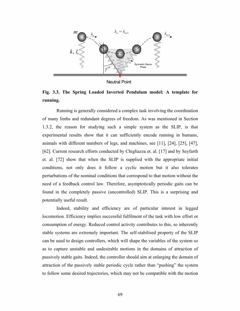
m

0, k l

Neutral Point

nx 1nx +

tdγSymmetric Stance

Phase

nx 1nx +=

Fig. 3.3. The Spring Loaded Inverted Pendulum model: A template for

running.

Running is generally considered a complex task involving the coordination

of many limbs and redundant degrees of freedom. As was mentioned in Section

1.3.2, the reason for studying such a simple system as the SLIP, is that

experimental results show that it can sufficiently encode running in humans,

animals with different numbers of legs, and machines, see [11], [24], [25], [47],

[62]. Current research efforts conducted by Chigliazza et. al. [17] and by Seyfarth

et. al. [72] show that when the SLIP is supplied with the appropriate initial

conditions, not only does it follow a cyclic motion but it also tolerates

perturbations of the nominal conditions that correspond to that motion without the

need of a feedback control law. Therefore, asymptotically periodic gaits can be

found in the completely passive (uncontrolled) SLIP. This is a surprising and

potentially useful result.

Indeed, stability and efficiency are of particular interest in legged

locomotion. Efficiency implies successful fulfilment of the task with low effort or

consumption of energy. Reduced control activity contributes to this, so inherently

stable systems are extremely important. The self-stabilised property of the SLIP

can be used to design controllers, which will shape the variables of the system so

as to capture unstable and undesirable motions in the domains of attraction of

passively stable gaits. Indeed, the controller should aim at enlarging the domain of

attraction of the passively stable periodic cycle rather than “pushing” the system

to follow some desired trajectories, which may not be compatible with the motion

69

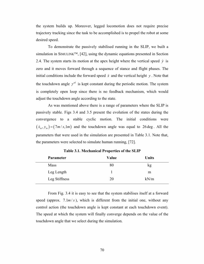
the system builds up. Moreover, legged locomotion does not require precise

trajectory tracking since the task to be accomplished is to propel the robot at some

desired speed.

To demonstrate the passively stabilised running in the SLIP, we built a

simulation in SIMULINK, [42], using the dynamic equations presented in Section

2.4. The system starts its motion at the apex height where the vertical speed is

zero and it moves forward through a sequence of stance and flight phases. The

initial conditions include the forward speed

y

x and the vertical height . Note that

the touchdown angle

ytdγ is kept constant during the periodic motion. The system

is completely open loop since there is no feedback mechanism, which would

adjust the touchdown angle according to the state.

As was mentioned above there is a range of parameters where the SLIP is

passively stable. Figs 3.4 and 3.5 present the evolution of the states during the

convergence to a stable cyclic motion. The initial conditions were

( ) (, 7 / ,1in in )x y m s= m and the touchdown angle was equal to . All the

parameters that were used in the simulation are presented in Table 3.1. Note that,

the parameters were selected to simulate human running, [72].

26deg

Table 3.1. Mechanical Properties of the SLIP

Parameter Value Units

Mass 80 kg

Leg Length 1 m

Leg Stiffness 20 kN/m

From Fig. 3.4 it is easy to see that the system stabilises itself at a forward

speed (approx. 7.1 ), which is different from the initial one, without any

control action (the touchdown angle is kept constant at each touchdown event).

The speed at which the system will finally converge depends on the value of the

touchdown angle that we select during the simulation.

/m s

70

Fig. 3.4. Passive convergence to a stable running cycle in the SLIP.

Fig. 3.5. Leg angle and leg length for the conditions of Fig. 3.4.

For a set of initial conditions (forward speed and apex height), there is a

value of the touchdown angle at which the system maintains its initial forward

speed, thus there is no transient motion involved. These conditions correspond to

71

starting the system at a point that lies on the periodic cycle and are referred to as

the neutral point. As Raibert pointed out, the neutral point corresponds to a

symmetric stance phase, where the lift-off and touchdown forward speed and

height are equal, [62], see Fig. 3.3. It is important to mention that symmetric

stance phase is a necessary and sufficient condition for cyclic motion in the SLIP.

For a rigorous proof of that fact, the reader is referred to [17], [69], [70]. For the

initial conditions used in Fig. 3.4, the touchdown angle that corresponds to a

neutral point is . 28.75deg

Raibert first observed that when the touchdown angle is smaller than its

value at the neutral point, for the given initial conditions of the cycle, the system

accelerates in the next step, [62], see Fig. 3.6. On the other hand, when the value

of the touchdown angle is greater than that corresponding to the neutral point, the

system decelerates in the next step.

m

0, k l

Neutral Point

Symmetric Lift-offcondition

tdγ

nx

1nx +

nx 1nx +<

m

0, k l

Neutral Point

Symmetric Lift-offcondition

tdγ

nx

1nx +nx 1nx +>

Fig. 3.6. Smaller touchdown angles (up) cause the system to accelerate by

decreasing its hopping height while larger touchdown angles (bottom) cause

the system to decelerate by increasing its hopping height.

72

As can be seen from Fig. 3.6, for a constant leg length and leg stiffness,

larger touchdown angles than those corresponding to the neutral point, result in

lift-off coming earlier than that predicted by the symmetric neutral point i.e. the

body spends more time during stance behind the leg than in front of it, see Fig.

3.6. This results in the hip being at a higher point at lift-off than at touchdown.

Therefore, during the stance phase, part of the kinetic energy was transformed to

potential energy resulting to deceleration. Exactly the opposite behaviour can be

observed when the touchdown angle is smaller than its value at the neutral point.

However, it is important to mention that this forward speed versus touchdown

angle relation is only part of the picture since it does not explain the self-

stabilisation property found in the SLIP, as it will be explained in the next

paragraph.

Based on the analytical derivation of a Poincaré map, a rigorous proof of

the passive stabilisation of the SLIP, has been given by Chigliazza et. al. in [17].

However, the mechanism that results in that self-stabilising property is not yet

well understood. Indeed, if we perturb the fixed point by changing the touchdown

angle, e.g. by decreasing it, then the system will accelerate in the first cycle. Thus,

at the second step the forward speed will be greater than that at the first, while the

touchdown angle will be the same. Normally, that would cause the system to

accelerate in the subsequent steps and finally fail due to toe stubbing (the kinetic

energy increases at the expense of the potential energy resulting to lower apex

heights). However, when the parameters are within the self-stabilisation regime,

the system does not fall. It adjusts its lift-off angle until it converges to a periodic

motion at higher forward speed where the stance phase is symmetric, see Fig. 3.5.

Notice that in converging to a periodic motion, the system passes through

successive steps of acceleration and deceleration, see x in Fig. 3.4. Therefore, not

only the touchdown but also the lift-off angle affects the energy distribution

between the forward and vertical motions, a fact that is not captured in Raibert’s

speed controller. Note, though, that the lift-off angle affects the motion in a

nonlinear way that totally depends on the dynamics of the system. Moreover, this

73

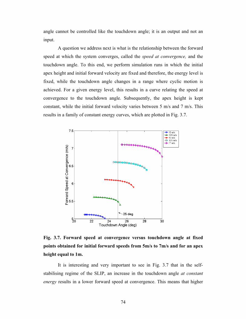
angle cannot be controlled like the touchdown angle; it is an output and not an

input.

A question we address next is what is the relationship between the forward

speed at which the system converges, called the speed at convergence, and the

touchdown angle. To this end, we perform simulation runs in which the initial

apex height and initial forward velocity are fixed and therefore, the energy level is

fixed, while the touchdown angle changes in a range where cyclic motion is

achieved. For a given energy level, this results in a curve relating the speed at

convergence to the touchdown angle. Subsequently, the apex height is kept

constant, while the initial forward velocity varies between 5 m/s and 7 m/s. This

results in a family of constant energy curves, which are plotted in Fig. 3.7.

Fig. 3.7. Forward speed at convergence versus touchdown angle at fixed

points obtained for initial forward speeds from 5m/s to 7m/s and for an apex

height equal to 1m.

It is interesting and very important to see in Fig. 3.7 that in the self-

stabilising regime of the SLIP, an increase in the touchdown angle at constant

energy results in a lower forward speed at convergence. This means that higher

74

forward speeds can be accommodated by smaller touchdown angles, which, at

first glance, is not in agreement with the global behaviour that higher speeds

require bigger (flatter) touchdown angles. This global behaviour is also evident in

Fig. 3.7, where it can be seen that forward speeds about, for example, 5 m/s

require touchdown angles in the range 21o-23.75o, while higher speeds such as

those about 7 m/s require larger touchdown angles, which lie in the range 25.75o-

30o Note that, the fact that globally fixed points at higher speeds require greater

(flatter) touchdown angles was reported by Raibert, [62], p. 40, and it was used to

control the forward speed of his robots based on a feedback control law. However,

Fig. 3.7 suggests that in the absence of control, i.e. when the system is open loop,

and for a constant energy level, a reduction in the touchdown angle results in an

increase of the speed at convergence. Therefore, one must be careful enough not

to transfer results from the case of systems actively stabilised to the case of

passive systems, because otherwise opposite outcomes from those expected will

result.

Fig. 3.7 also shows the domain of attraction of the fixed points. As can be

seen, at higher forward speeds the system becomes less sensitive to perturbations

of the nominal conditions i.e. larger variations in the touchdown angle are

tolerated by the system. This is in agreement with recently obtained results from

biomechanics, where at high speeds the mechanical system itself can tolerate

larger deviations from the fixed point conditions, [25], [36]. McGeer has also

observed this result in the context of passive bipedal running, where higher speeds

improve the stability, [43]. In Chapter 4, where the stability of passively generated

bounding motions is studied, analogous conclusions have been obtained.

3.4. Existence of a Passive Bounding Gait

Inspired by the passive stability of the SLIP system, [17], which was briefly

presented in Section 3.3, and by the passive dynamic walker McGeer constructed

more than a decade ago, [43], we will investigate in this section the passive

dynamics of Scout II in the bounding running presented in Section 2.2, Fig. 2.4.

With the term passive dynamics, we mean the unforced response of the system

75

under a set of initial conditions. The goals of the analysis are to determine the

conditions required to permit steady state cyclic motion, to understand the

fundamentals of the bounding gait followed by the robot and to find ways to apply

these results to improve the performance of Scout II. The practical motivation for

studying the passive bounding is power efficiency. Indeed, if the cyclic motion is

generated passively then the actuators have less work to do to maintain the motion

since they do not “push” the robot towards motions that are against its natural

dynamics. Furthermore, if there are operating regimes where the system is

passively stable then active stabilisation is not required and the motors of the

robot will only compensate for energy losses. The benefits of a control approach

based on the passive dynamics of the system are multiple, especially in

simplifying the mechanical electrical and electronic design and in extending the

operational range of the robot.

In this section, we introduce a template for studying the bounding and

pronking gaits in Scout II. It is important to mention here that there is extensive

literature on the SLIP model, not only because it captures the basic properties of

legs in running but also because its model is simple enough to possibly allow for a

mathematically tractable solution. However, SLIP does not describe the pitching

motion, which is a significant factor for stability. Indeed, the pitching motion

determines which leg, front or back, will hit the ground first, a fact that can cause

significant difference in the motion. Therefore, there is space for the development

of a simple model to study the quadrupedal running gaits in the sagittal plane.

Note that, to the best of the author’s knowledge, the only model for quadrupedal

running studied in the literature is by Berkemeier in [9], but it does not take into

account the forward motion (running/hopping in place) and it is not passive.

3.4.1. Definition of the Bounding Return Map

The passive behaviour of Scout II will be investigated by numerically

constructing a return map to describe the bounding gait. The model considered is

passive and conservative: no energy is added or lost. The model is basically the

same with the one developed in Section 2.5 with the difference that there is no

76

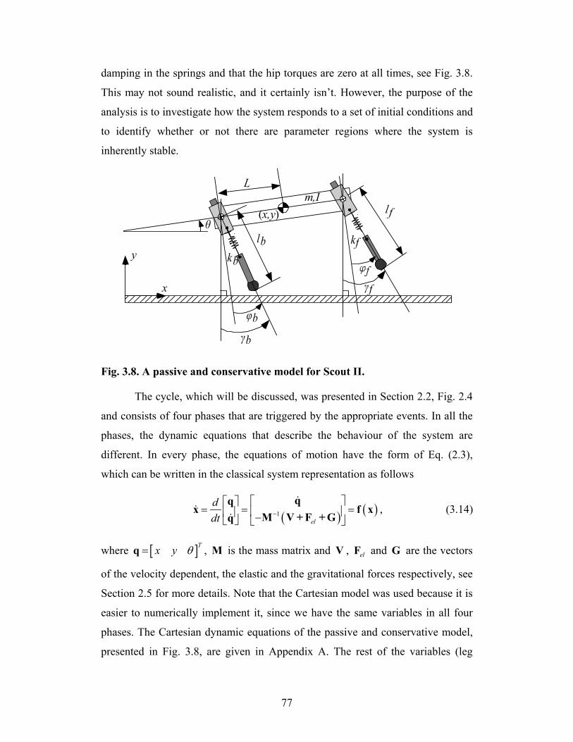
damping in the springs and that the hip torques are zero at all times, see Fig. 3.8.

This may not sound realistic, and it certainly isn’t. However, the purpose of the

analysis is to investigate how the system responds to a set of initial conditions and

to identify whether or not there are parameter regions where the system is

inherently stable.

L

lf

φbγb

γf

θlb

kb

kf

(x,y)m,I

x

y

Fig. 3.8. A passive and conservative model for Scout II.

The cycle, which will be discussed, was presented in Section 2.2, Fig. 2.4

and consists of four phases that are triggered by the appropriate events. In all the

phases, the dynamic equations that describe the behaviour of the system are

different. In every phase, the equations of motion have the form of Eq. (2.3),

which can be written in the classical system representation as follows

( ) ( )1el

ddt −

= = = −

qqx

M V + F + Gq f x , (3.14)

where [ ]Tx y θ=q , is the mass matrix and , and G are the vectors

of the velocity dependent, the elastic and the gravitational forces respectively, see

Section 2.5 for more details. Note that the Cartesian model was used because it is

easier to numerically implement it, since we have the same variables in all four

phases. The Cartesian dynamic equations of the passive and conservative model,

presented in Fig. 3.8, are given in Appendix A. The rest of the variables (leg

M V elF

77

lengths, leg angles) are found by kinematic closure equations presented in Section

2.5. Cycle calculations involve several coupled nonlinear differential equations

with a formidable number of terms. The complexity of the equations precludes

finding the return map analytically, thus we resort to numerical evaluation of the

return map, which is discussed in this section.

To define the return map, we first consider a convenient point in the

bounding running cycle. We use the apex height in the double leg flight phase.

We could select any other point in the cycle, however the selection of the apex

height allows for the touchdown angles of both the front and back virtual legs to

explicitly appear in the definition of the return map as kinematic inputs available

for control. Selection of points in the cycle where one or both the legs are on the

ground, such as touchdown or lift-off points, would result to the definition of a

return map where one or both the touchdown angles would be part of the state

vector and not inputs. This will be apparent later. We define the Poincaré section

to be the hyperplane

{ }60 0| 0, ,b fy l l l lΣ = ∈ = = = ⊂x 5

l

, (3.15)

where the conditions l and l0b l= 0f = were added to show that the robot is in

double leg flight, since becomes zero not only at the apex but also at the lowest

height. The system is at its apex when its orbit pierces the hyperplane . To

define the Poincaré map it is necessary that

y

Σ

Σ satisfies the transversality

condition, Eq. (3.9), i.e. Σ must transversal to the flow. Mathematically this

means that the dot product of the vector field and the hyperplane’s normal must

never be zero. In the coordinates ( ), , , x y , , x yθ θ the hyperplane normal

direction is simply [ ]0 0 0 0 1 0 T

0g −

=

0 0x θ=

n , while the vector field at the apex

height is , since when the robot is in double flight

phase it follows a ballistic trajectory, as it was described in Section 2.5.1. Thus,

we have

( )f xT

( ) 0T g= − ≠n f x , (3.16)

78

which means that the transversality condition is satisfied.

Since the apex height is considered the reference point, we seek a function

that maps the apex height of the n th stride to the apex height of the ( )

)

5

1n + th stride

i.e. the return map. The states at the n th apex height constitute the initial

conditions for the cycle, based on which we integrate the double flight phase

equations, until the back leg touchdown event occurs. The back leg touchdown

event triggers the back leg stance phase, whose dynamic equations are integrated

using as initial conditions the final conditions of the previous phase. Note that if

we were considering that the legs have non-zero mass then the initial conditions

for the back leg stance phase would have been calculated from the final conditions

of the double leg flight phase using the impact equations. However, since the legs

are considered massless there are no transition equations involved and the final

conditions of one phase are the same as the initial conditions of the next. By

successively integrating forward the dynamic equations of all the phases

according to the events that happen, we calculate the value of the state vector at

the ( 1n + th apex height, which is the value of the return map calculated at the n th

apex height. If the state vector at the new apex height is identical to the original,

then the cycle is repetitive. We seek for such “re-entry” conditions.

The return map is defined as a vector function mapping

apex height conditions from stride to stride

5 2: × →P

n 1n + ,

1

,tdbtdf n

n n

x xy y

x x

γθ θ

γ

θ θ+

=

P , (3.17)

where tdbγ , td

fγ are the touchdown angles of the back and front legs respectively

with respect to the vertical, see Fig. 3.8. To avoid confusion, it must be mentioned

that the leg angles change during the cycle when the legs are in stance, however

their touchdown values remain constant for a fixed point. That means that in the

flight phase the leg angles are adjusted kinematically to obtain their touchdown

79

values. It can be seen that although the touchdown angles are not part of the state

vector of the return map, they directly affect the value of the map. This is because

the conditions describing the touchdown events, Eqs. (2.48), are functions of the

touchdown angles and they affect the initial conditions of each of the stance

phases. This is a direct consequence of the assumption of the massless legs as it

was analytically described in Section 2.5.

Eq. (3.17) has the standard form of a nonlinear discrete time system

( )1 ,n n+ =x f x un , (3.18)

where is the state vector and u includes the inputs, which, in our case, are the

touchdown angles. As was mentioned above, the fact that both the touchdown

angles explicitly appear in the above representation, lead us to choosing the apex

height as a reference point. The same holds for any other point in the double leg

flight phase, however we selected the apex height event as a reference point

because of its physical meaning. From the above it is apparent that the touchdown

positions of the legs are extremely important parameters that drastically affect the

system’s motion. Indeed, they provide “cheap” controls, since in Scout II it is

very easy to place the legs at a desired touchdown position during the flight phase.

These controls can be used to improve the stability properties of the fixed points

of the Eq. (3.17), which, as was seen in Section 3.2, is equivalent to the stability

properties of the closed orbit of the continuous time dynamic system (3.1). It is

also important to mention that the coordinate is not included in the arguments

of the return map because Eq. (3.17) maps apex height to apex height where is

always zero (the dimension of a return map is equal to the dimension of the

system minus one).

x

y

y

Since x is the horizontal coordinate of the COM, it will never be identical

between two successive apex height points. This is because the forward distance

traveled during one stride is always non-zero for non-zero forward speeds.

Therefore, x will be excluded from the procedure followed to find the fixed

points of the return map, thus reducing the searching space by one dimension.

Therefore, we search for fixed points of the function , 4 2: × →P 4

80

1

,tdbtdf n

n n

y y

x xγθ θγ

θ θ+

=

P . (3.19)

It is important to note here that in calculating the return map only one

specific sequence of events and thus of phases was considered. This sequence was

described in detail in Section 2.2, Fig 2.4, and it was chosen because the robot

shows some “preference” in following that gait. A more general approach would

have been to implement the search scheme to take into account other possible

sequences of the phases, which result in different phases, e.g. symmetric bounding

motion where flight occurs after back leg stance double instead of double stance

or pronking. Generalising the implementation of the method to include gaits other

than the specific bounding gait examined here will be a subject of future

investigation.

3.4.2. Searching for Fixed Points

We want to find an argument of Eq. (3.19) that maps onto itself, i.e. we want to

solve the equation

x

( ) ( )− =F x x P x 0 , (3.20)

for all the values of touchdown angles. Solution of Eq. (3.20) is by no means

guaranteed, however existence seems to be the rule rather than the exception. It is

important to mention that when solutions exist they are not always unique,

furthermore they are not well spaced. To calculate an individual solution one has

to specify the values of the touchdown angles along with the values of the model

parameters and solve Eq. (3.20).

The search space is 4-dimensional with two free parameters, since for

different values of touchdown angles, different solutions may be obtained. To

describe as a nonlinear function by analytically integrating the dynamic

equations over this space is to do injustice to its rather unfortunate complexities,

so the search will be conducted numerically. We will use the Newton-Raphson

P

81

method, where an initial guess for the fixed point is given and then updated based

on the following scheme. Define the gradient matrix (Jacobian) of the return map,

T

y xθ θ ∂ ∂ ∂ ∂

∇ = ∂ ∂ ∂ ∂

P P P PP . (3.21)

For small changes in the state variables (keeping the touchdown angles as

parameters), the change in is approximated by its Taylor series, P

( ) ( ) ( ) ( )O+ ∆ = + ∇ ∆ + ∆P x x P x P x x x , (3.22)

where are higher order terms, which for the purpose of our analysis are

considered negligible. Therefore, we have

(O ∆x)

( ) ( ) ( )( ) ( )1n n n n

−∇ ∆ = − ⇒ ∆ = − ∇ − n F x x F x x I P x P x x , (3.23)

where is the value of the states of the return map calculated at the nnx th apex

height. Based on Eq. (3.23) we have the following update scheme, given an initial

guess 0nx ,

( )( ) ( )11k k k k

n n n n n

−+ k = + − ∇ − x x I P x P x x , (3.24)

where the index corresponds to the n n th apex height and the index

corresponds to the number of iterations.

k

To find a solution one evaluates Eq. (3.24) iteratively until convergence.

For the results presented here convergence is achieved when the error between k

nx and 1kn

+x is smaller than 1 6e − . The value of at P knx

P

is calculated through

the numerical integration of the dynamic equations during a complete cycle. Each

iteration involves nine evaluations of the return map . One corresponds to

calculating at the nominal point P knx and eight to get the gradients, which are

found numerically. To calculate the components ix∂ ∂P of the gradient matrix

, we need four evaluations of at ∇P P kn d−x x (fore of the nominal point) and

four at kn d+x (aft of the nominal point), where is obtained by perturbing x dx

82

each of components of x , 1, , 4i = … , by some small scalar quantity dx . In

implementing this scheme we used 1dx e 6= − . Then central difference

approximation is used to evaluate numerically the corresponding derivatives, e.g.

for some component ix of the state vector x we have

(,..., ,..., ,...,2

ix dx xx d

+ −P P

e

P

( ) )1 4 1 ,...,i

i

x x x dx xx

−∂=

∂P . (3.25) 4

Apparently, Eq. (3.24) requires quite a bit of calculation! Fortunately, if the initial

guess is reasonable and a solution exists, the above method finds it usually in less

than eight iterations. Fig. 3.9 presents a flow chart showing the search procedure.

To implement the above method we used MATLAB. Integrations of the

equations of motion have been done using the adaptive step Dormand-Price

integration method (MATLAB’s ode45 function, [42]) with 1 and 1 7

relative and absolute tolerances respectively. It is worth mentioning that

MATLAB offers a very useful feature for event-based integration of differential

equations.

6e − −

3.4.3. Finding Fixed Points

In finding fixed points, the method described in Section 3.4.2, see Fig. 3.9, was

employed. Initially we specify the values of the touchdown angles and some

initial guess and then using Eq. (3.24) we update the initial guess until

convergence. One approach is to specify the initial guess and the touchdown

angles by randomly selecting values within some reasonable range. This approach

is unbiased and can reveal fixed points, which might otherwise go unnoticed.

Surprisingly we were able to find many fixed points of the return map , for

different initial guesses and different touchdown angles. The fixed points found

randomly exhibited strong dependence on the initial guess and on the touchdown

angles, so a more systematic way for generating fixed points had to be employed.

Before presenting a more systematic approach for finding fixed points, we

describe some very useful properties concerning the symmetry of the bounding

motion that corresponds to the fixed points found above.

83

END

START

NO

YES

Evaluation of the Return Map

( )1 ,k k kn n nx u< > < > < >

+ =x P

Return Map at thefore point

( )k kn n d< > < >

−= −x x x

( ) ( )( )1 ,k k kn n nx u< > < > < >

+ − −=x P

Update the Guess

( ) ( )1 4 1 4,..., ,..., ,..., ,...,2

i i

i

x x dx x x x dx xx dx

+ − −∂=

∂P PP

( )( ) ( )11k k k k k

n n n n n

−+ = + − ∇ − x x I P x P x x

Return Map at theaft point

( )k kn n d< > < >

+= +x x x

( ) ( )( )1 ,k k kn n nx u< > < > < >

+ + +=x P

k=1

k=k+1

Initial EstimateTk k k k k

n n n n ny xθ θ< > < > < > < > < > = x

( ) ( )Tk kk td td

n b fn nγ γ

< > < >< > = u

( ) ( )( ) 611,...,4

max 10k kn ni

i i< > < > −+=

− <x x

Fig. 3.9. Flow chart presenting the numerical algorithm for calculating the

fixed points of the return map.

In Fig 3.10 we present the plots showing the evolution of the states during

one cycle of the bounding motion corresponding to a fixed point. The initial guess

was , the corresponding

fixed point is ( )( ) ( )o, , , , , 0.38 ,0,1.4m/s,120 /s ,16 ,12td td o o

b fy x mθ θ γ γ =

( )/s ,16 ,12o oo, , , , , 0.32 ,0,1.42m/s,143.75td tdb fy x mθ θ γ γ = .

It is apparent from Fig.3.10 that state values at the end of the cycle are

identical to the state values at the beginning of the cycle. Note also that during

double flight, the forward speed x is constant, since energy losses in the double

flight phase due to air resistance have not been modeled. The same holds for the

84

pitch rate θ because the legs are considered massless, so the model does not

capture changes in the pitch due to leg motions during double leg flight. It is

important to note that the pitch angle θ is zero at the apex height. This property

has been observed for all fixed points found. As far as the simulation can be used

to draw conclusions for the properties of the fixed points, it seems that the pitch

angle is always zero at the apex height.

Fig. 3.10. Evolution of the state variables during one bounding cycle. The

vertical lines show the events: back leg touchdown, front leg touchdown,

back leg lift-off and front leg lift-off.

Fig. 3.11 presents the leg lengths and the leg angles for the back and front

virtual legs for the same fixed point during one cycle. It can be seen that, although

the leg angle changes throughout the stance phase, its touchdown value remains

constant from one stance phase to another. To maintain cyclic motion, the leg is

brought to its touchdown position kinematically during the flight phase. Careful

inspection of Fig. 3.11 reveals another important property of the fixed points. As

85

we can see, the touchdown angle of the front leg is equal to the negative of the

lift-off angle of the back leg while the touchdown angle of the back leg is equal to

the negative of the lift-off angle of the front leg.

Fig. 3.11. Evolution of the leg length and the leg angles.

This result, in combination with the fact that the pitch angle is always zero

at the apex height, reveals a symmetric behaviour, which initially was not

expected because of the double stance phase of the bounding cycle. However, as

shown in Figs. 3.10 and 3.11 our passively generated bounding motion exhibits

symmetric properties about the middle of the double stance phase. This is always

true for all the fixed points found randomly by following the method described

above. It is known that conservation of quantities –our model is passive without

energy losses so energy is conserved– results in symmetric motions. Remember

also that in the case of the SLIP model, a necessary and sufficient condition for

fixed points is the symmetric stance phase, i.e. the lift-off angle is equal to minus

the touchdown angle. This has been proved using both analysis and simulation,

see [17], [69], [70].

86

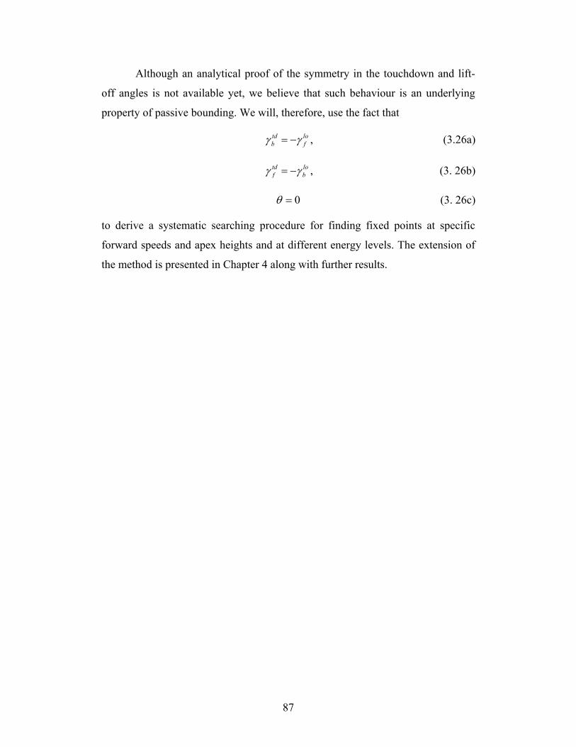
Although an analytical proof of the symmetry in the touchdown and lift-

off angles is not available yet, we believe that such behaviour is an underlying

property of passive bounding. We will, therefore, use the fact that

td lob fγ γ= − , (3.26a)

td lof bγ γ= − , (3. 26b)

0θ = (3. 26c)

to derive a systematic searching procedure for finding fixed points at specific

forward speeds and apex heights and at different energy levels. The extension of

the method is presented in Chapter 4 along with further results.

87

Chapter 4

Passive Dynamics of Scout II: Results

4.1. Introduction

In this chapter, the searching procedure for finding fixed points described in

Chapter 3 is further developed and improved resulting in a more systematic way

of generating continuums of fixed points. Using this more systematic procedure,

conclusions on how the system responds under a set of initial conditions can be

drawn. In Chapter 3, we briefly described the passive dynamics of the SLIP.

Surprisingly, there are regions of parameters where the system is stable without

the need of a closed loop controller. The purpose of the analysis in this chapter is

to quantify the properties of passively generated periodic motion for Scout II and

to search for regions where the system can passively tolerate departures from the

fixed points.

The major question is whether there exists a regime, where the system

tolerates perturbations from the nominal conditions without requiring any closed

loop control law. The existence of this regime raises an important “philosophical”

question: How much feedback is necessary for developing control laws to

stabilise the system? Is it possible to derive controllers, which will keep the

system in the self-stabilised regimes? The answers to these questions are not yet

available. However, the existence of passively stabilised behaviours suggests that

clock based feed-forward control laws can excite the dynamics of the robot

appropriately to exploit the inherent stability of the system. The added feedback

88

can improve the robustness of those controllers. Therefore, we believe that the

results presented in this chapter constitute a beginning in the right direction.

It should be mentioned here that a review of the related literature leaves

one with the impression that the problem of dynamically stable legged locomotion

does not fit well in the framework of modern robot control theory. This is mainly

because the equations of motion of the system are different in every phase and

thus different dynamics apply at each stage of the gait. Studying each of these

phases separately cannot produce a controller to stabilise the system. This is

because stability must be obtained for the whole cycle and not for each phase,

which can be unstable.

The structure of this chapter is as follows: In Section 4.2 we expand and

improve the method presented in Section 3.4 to find passively generated cyclic

trajectories for specific forward speeds and apex heights. Some conclusions on

pronking and bounding are also given. In Section 4.3, we characterise the local

stability properties of the fixed points and regions where the system can be

inherently stable are identified.

4.2. Symmetric Periodic Trajectories

As was mentioned in the previous chapters, one of the main difficulties in legged

locomotion is that the task cannot be defined in terms of some desired trajectories

in the Cartesian or in the state space. The task of running in Scout II can be

formulated loosely to require an asymptotically stable fixed point of its discrete

return map with

• a specific (average, forward) speed

• a certain gait (e.g. pronking, bounding)

• minimal energy consumption.

In other words, we first want to find if there exist fixed points at specific

desired speeds and apex heights. This is achieved by proper use of the searching

scheme described in Section 3.4. According to this scheme, the search state vector

includes the variables that are updated during the searching process, while the

search input contains the variables that are determined at the beginning of the

89

search and remain constant during it. Therefore, the scheme of Section 3.4 is

modified here so that the forward speed and apex height become its input

parameters, which are specified arbitrarily, while the touchdown angles are now

considered to be states of the searching procedure, i.e. variables to be determined

from it. By doing so, the search space is now spanned by the states

* Ttd tdb fθ θ γ γ = x , (4.1)

while the vector of the parameters (“inputs” to the search scheme) is

[ ]* Ty x=u . (4.2)

It is important to note that the above rearrangements in the arguments of the

return map are performed to ease the implementation of the search scheme and do

not affect the physics of the problem.

The searching procedure starts by specifying an initial guess for θ , θ , tdbγ

and tdfγ and giving some desired values to and y x . The differential equations

describing the dynamics of the phases are then integrated to derive the return map.

Note that the numerical integration of the equations of motion starting from the

apex height event, results in the calculation of lift-off angles and not of the

touchdown angles of the legs at the next apex height event. Indeed, at the end of

the front leg stance phase, the legs are at their lift-off positions, and subsequent

integration of the double leg flight dynamic equations will leave the leg angles

unaltered. This is a direct consequence of the assumption of massless legs.

Therefore, we have the following equation relating successive apex height events

1

,lo tdb b nlo tdf fn n

yx

θ θθ θγ γγ γ

+

=

P , (4.3)

where it can be seen that application of the function , results in the lift-off

angles and not in the touchdown angles. Thus, to calculate the gradients needed to

P

90

implement the Newton-Raphson scheme the lift-off angles must be “mapped” to

touchdown angles based on the symmetry described in Section 3.4.3,

( ) ( )1 1

td lob n

γ γ f n+ += − , (4.4a)

( ) ( )1

td lof n

γ γ1b n+ +

= − . (4.4b)

Then, by using the Newton-Raphson algorithm as in Section 3.4.2, we update the

initial guess by moving along a direction in the search space which decreases the

difference between x and *n

*1n+x

e

, until convergence is achieved according to some

numerical accuracy (we used 1 6− in all the results shown here).

Note that the above search scheme does not explicitly ensure that a fixed

point the following equations between two successive strides must hold,

1ny + ny= , (4.5a)

1n nx x+ = . (4.5b)

Instead, in the new search scheme, we required Eqs. (4.4) to hold. However,

examination of the search results shows that the conditions described by Eqs.

(4.5) are also satisfied. This numerical fact shows that the conditions described by

Eqs. (4.4) are equivalent to the conditions for the existence of a fixed point. Note

that this behaviour is analogous to that of the SLIP model, where the symmetric

stance phase is a condition for a fixed point, [17], [70].

Fig 4.1 presents fixed points for a forward speed of 1 m/s, an apex height

equal to 0.35 m and varying pitch rates. In interpreting this plot, it is useful to note

that the pitch rate is essentially a measure of the total energy for fixed forward

speeds and apex heights. Therefore, the fixed points presented in Fig. 4.1 do not

correspond to the same energy level. As we can see there is a continuum of fixed

points, which follows an “eye” pattern, accompanied by two external branches.

The existence of the external branch means that there is a range of pitch rates

where two different fixed points for the same forward speed, apex height and

pitch rate exist. This is quite surprising since the same total energy and the same

distribution of that energy among the three modes of the motion -forward, vertical

91

and pitch- results in two different motions depending on the touchdown angles.

Fig. 4.2 presents the two different bounding motions that correspond to fixed

points on the external and the internal branches. The fixed points that lie on the

internal branch correspond to a bounding motion where the front leg is brought in

front of the torso, while the fixed points that lie on the external branch correspond

to a bounding motion where the front leg is brought towards the torso’s COM.

Fig 4.1. Fixed points for 1m/s forward speed and 0.35m apex height.

A basic conclusion from Fig. 4.1 is that the back leg touchdown angle is

always greater than the front leg touchdown angle in all the pitch rates at which

fixed points can be found. Now recall that, 0θ = always at the apex height (see

Fig. 3.10 in Section 3.4.3). As can be seen from Fig. 4.1, as we approach the

vertical axis, where , the touchdown angles of the front and back legs tend

to become equal. It is interesting to note that a gait with

0θ =

0θ = , and equal

touchdown angles for the front and back legs corresponds to the pronking gait,

where the front and back legs strike the ground almost in unison. Therefore,

points which are close to the vertical axis correspond to pronking-like motions.

Useful conclusions concerning the stability of the bounding and the pronking gaits

will be discussed in the next section.

0θ =

92

Fig. 4.2. Snapshots showing the motion of Scout II for the internal branch

and the external branch fixed points. The plot on the left is a smaller version

of Fig. 4.1.

To further investigate the passive behaviour of the robot, we implemented

the searching procedure for different forward speeds keeping the apex height the

same. In Fig 4.3 the fixed points for forward speeds varying from 1.5 to 4 m/s and

for constant apex height, 0.35 m, are presented. It can also be seen that at higher

speeds the “eye” pattern shown in Fig 4.1 shifts to higher values of the touchdown

angles. This can be better seen in Fig. 4.4. Moreover, note that we were not able

to find external branches of fixed points at speeds higher that 1m/s.

Fig. 4.3. Formations of fixed points for apex height 0.35 m and forward

speeds to 1.5 m/s. [ ]min max,E E is the range of the total energy of the fixed

points.

93

Note also that the fixed points shown in Fig. 4.3 correspond to different

energy ranges, which do not overlap, a fact that is particularly important for

designing controllers. Indeed, it would be useful to find continuums of fixed

points at different speeds with the same total energy. This is because such a

searching procedure would result in curves of the touchdown angles as function of

the speed, , which could be directly used as a definition for the

“desired” behaviour. Based on that desired behaviour, a feedback control law

could be designed to adjust the legs according to

( )td u xγ =

( )td u xγ = for a specific energy

level.

Fig 4.4. Formations of fixed points for apex height 0.35m and speeds varying

from 1.5 to 3.5 m/s.

However, continuums of fixed points with different forward speeds at the

same total energy cannot be found for reasons that will be explained next.

Keeping the energy constant and searching at different speeds leaves us with two

degrees of freedom in the searching scheme: the apex height and the pitch rate y

θ . It is reasonable to keep the apex height at a desired value and let θ be

specified by the rest of the variables (speed, apex height and energy). However, a

94

searching procedure that would keep the energy and the apex height constant and

that would search at different forward speeds cannot result in a tdx γ− curve over

a large range of speeds, which would be suitable for implementation. Indeed, the

total energy at the apex height is

)mgy− (2 2 2 21 1 22 2

E mx I mgy mx I Eθ θ= + + ⇒ + = , (4.6)

thus keeping the total energy and the apex height constant results in ellipses on

the x θ− plane,

2 E mgyxm

cosξ− =

, (4.7a)

2 E mgyI

sinθ ξ− =

, (4.7b)

where [ ]0, 2ξ π∈

E

. These ellipses are presented in Fig. 4.5 plotted at different

energy levels and for apex height 0.35y m= .

Fig. 4.5. Constant energy levels for energies between 70J and 200J. The

markers are the fixed points found at speeds from 1.5 to 3.5 m/s.

95

From Fig. 4.5 we see that, at higher energies, the constant energy curves

almost become straight lines, i.e. they almost coincide with the constant forward

speed curves. In other words, very small changes in the speed must be

accompanied by much larger changes in the pitch rate to keep the energy constant

during the search. That means that if we select an energy level and start searching

for fixed points at that energy level by changing the speed, then, even if we find

more than one fixed points at that energy, their forward speed will be almost the

same. In that case, a plot of the front and back leg touchdown angle as a function

of the forward speed would not be useful for control. In general, large changes in

the pitch rate slightly affects the speed when the total energy and the apex height

are kept constant. Note that an alternative would be to keep θ constant and search

for various speeds changing accordingly to keep the energy level constant.

However, from a practical point of view, it is not useful to search for fixed points

by keeping

y

θ constant, because we do not know which value to select.

Finally, it is important to mention that whether or not the method

described above finds all the fixed points is an open question. Unfortunately, we

will not be able to make sure that there are no other branches of fixed points for

the specific conditions. Development of analytical instead of numerical

approximations might give some more insight to that issue, however these

solutions are currently under investigation.

4.3 Stability Analysis

The existence of passively generated bounding running cycles is by itself a very

important result since it shows that an activity so complex as bounding running

can be simply a natural motion of the system. However, in real situations the

robot is continuously perturbed, therefore, if the fixed point were unstable, then

the periodic motion would not be sustainable. It would therefore be important to

study the stability properties of the fixed points found above and to design

controllers to improve the robustness of the system against perturbations. In this

96

section, we characterise the stability of the fixed points using local stability

analysis i.e. using the eigenvalues of the linearised return map.

The stability analysis is based on linearising the nonlinear map about a

fixed point. A set of linearised equations specifies how a perturbation on the

steady cycle propagates from one cycle to the next. The problem of stability in

discrete-time systems, such as the return map derived in Section 3.4, Eq. (3.19), is

different from the continuous-time case, because of the different stability domain

in the complex plane. The left half of the complex plane in the continuous time

systems is replaced by the inside of the unit circle. Calculating the system’s

eigenvalues and checking whether or not they are inside the unit circle can verify

stability for discrete time systems. Therefore, to investigate stability, we assume

that the apex height states are perturbed from their steady-cycle values x , by

some small amount ∆ . The model that relates the deviations from steady state,

i.e. the incremental or small-signal model, is

x

( ) ( )1 1

, ,n n n n+ +

∂ ∂∆ = ∆ + ∆ ⇒ ∆ = ∆ + ∆

∂ ∂x=x u=u

P x u P x ux x u x A x

x u n nB u , (4.8)

with ∆ = −x x x , ∆ = −u u u . For small perturbations, the apex height states at the

next stride can be calculated by Eq. (4.8), which is a linear difference equation. If

all the eigenvalues of the system matrix A have magnitude less than one, then the

periodic solution is stable and disturbances decay in subsequent steps. If not, then

disturbances grow and eventually repetitive motion is lost.

Fig. 4.6 shows the eigenvalues of matrix for forward speed 1 m/s and

apex height 0.35 m. As it was expected, one of the eigenvalues is always located

at one, representing the fact that the system is conservative. Indeed, consider the

new coordinate on the Poincaré section

A

Σ , which is defined by Eq. (3.15),

2 21 12 2

E mx I mgθ= + + y , (4.9)

which corresponds to the system’s total energy defined at apex height. If we

eliminate the variable which corresponds to the apex height, by substitution of y

97

21 1 12 2

y E mx Img

2θ= − −

(4.10)

in the return map defined by Eq. (3.19), then the linearisation of the map about a

fixed point (equilibrium point) should look like

11 12 13

21 22 23

31 32 331

1 0 0 0 0 0* * ** * ** * *

tdbtdf n

n n

E Ej j jj j jx xj j j

γθ θγ

θ θ+

∆ ∆ ∆∆ ∆ = + ∆∆ ∆ ∆ ∆

, (4.11)

where are values to be determined and the * elements are not relevant for

stability considerations. From Eq. (4.11) it is easy to see that one of the

eigenvalues will always be at one, since the energy is conserved. Note that from a

control point of view this is an uncontrollable mode. Indeed, there is no feedback

law that can change the position of this eigenvalue since that would make the

system non-conservative.

ijj

Fig. 4.6. Root locus showing the paths of the four eigenvalues as the pitch rate

varies from low values (blue) to high values (red). The same pattern is

observed for different forward speeds and apex heights.

98

The behaviour of the other three eigenvalues is depicted in Fig. 4.6. Two

of the eigenvalues start on the real axis and as θ increases they move towards

each other. At some point, they meet inside the unit cycle, they split, leaving the

real axis and finally they move towards the rim of the unit circle. The problem is

with the third eigenvalue, which starts at a high value and moves towards the unit

circle but it never gets into it, for those specific values of forward speed and apex

height. Since this eigenvalue stays outside of the unit circle for every θ , there is

no region of parameters where the system is passively stable for speed 1 /x m s=

and apex height . 0.35y m=

Fig. 4.7 shows the magnitude of the larger eigenvalue at different forward

speeds. It can be seen that, as the forward speed increases, stability is improved.

Careful inspection of Fig. 4.7 reveals that, for sufficiently high forward speeds

and pitch rates, the larger eigenvalue enters the unit circle while the other two

eigenvalues remain well behaved. Therefore, there exists a regime where the

system can be passively stable. That means that the system can tolerate possible

small perturbations of the nominal conditions without any control action taken!

This fact could provide a possible explanation to why our Scout II robot can

bound, without the need of task-based state feedback, using very simple control

laws that only excite its natural dynamics. This fact is in agreement with recent

research in the context of biomechanics, which shows that when animals run at

high speeds, [25], [36], passive dynamic self-stabilisation from a feed-forward,

tuned mechanical system can reject rapid perturbations and simplify control. As it

was mentioned in Section 3.3, the fact that stability improves as the speed

increases, has also been observed in the SLIP. McGeer also discovered analogous

behaviour in his passive bipedal running work, [43].

The implications of the fact that there exists a regime, in which Scout II

can passively stabilise itself, can facilitate the design of control laws for

dynamically stable legged locomotion that exploit this self-stabilisation regime.

Indeed, the purpose is to develop controllers, which would enlarge the domain of

attraction of the stable fixed points thus resulting in improved robustness with

reduced control activity. This is important for reducing energy consumption. Note

99

also that the control action is entirely taken during flight, a fact that allows for

higher energy efficiency, since placing the legs at the desired positions does not

require large torques.

Fig. 4.7. Norm of the larger eigenvalue at various pitch rates and for forward

speeds between 1.5 and 4m/s. The apex height is 1m.

Fig. 4.8 shows how the norm of the maximum eigenvalues changes as a

function of the pitch rate, at different apex heights keeping the forward speed

constant at 3 m/s. It can be seen that the lower the apex height is, the less unstable

the system is. Indeed, as was seen in Fig. 4.7, for an apex height of 0.35 m, the

forward speed has to be greater than 3.5m/s for the motion to be stable. On the

other hand, when the apex height is 0.32m and the forward speed greater than

2.8m/s, the system enters the self-stabilisation regime. Therefore, greater forward

speeds and lower apex heights contribute to the stability of the open loop system.

This fact has been observed in both simulations and experiments, where for a

given energy level, the system stabilises itself at high pitch rates and low apex

heights, approximately equal to the leg length.

100

Fig. 4.8. Norm of the larger eigenvalue at various pitch rates and for apex

heights between 0.32 and 0.37m. The forward speed is 3m/s.

It is important to note that, as was seen in all the above plots (Figs. 4.6, 4.7

and 4.8), the larger eigenvalue obtains its maximum values when the pitch rate θ

is small. Recall that the region where θ takes small values corresponds to

pronking-like motion, where both the front and back legs hit and leave the ground

in unison. Thus, we can conclude that pronking-like motions are more unstable

than bounding, which corresponds to higher pitch rates. This is a very useful

result, which shows why Scout II ‘prefers’ to bound rather than pronk. Moreover,

it suggests that intense control action has to be taken, to force the robot to pronk

and that simple control laws, which only excite the dynamics of the system, are

unlikely to produce stable pronking motion.

Furthermore, Fig. 4.7 shows that, at low pitch rates, i.e. pronking-like

motions become “more unstable” as the speed increases. This shows that pronking

is even more difficult to get at high speeds contrary to bounding, which, as was

mentioned above, is passively stable at high speeds. These results suggest that

101

pronking is not the proper gait for Scout II when efficient, high-speed locomotion

is needed. Moreover, pronking controllers should be derived to “push” the system

to follow this gait, thus we can conclude whether or not one should attempt to

study pronking.

The fact that the robot shows a preference to bounding was also observed

experimentally, see [55], [57], [78], and it is not surprising. Indeed, the concept of

the dimensionless moment of inertia can be used to understand why the robot

shows preference for bounding. The dimensionless moment of inertia is

defined by the equation, [52],

j

2

IjmL

= , (4.12)

where I is the moment of inertia of the body, m is the mass of the body and is

half the hip spacing. Applying Eq. (4.12) for Scout II, based on the data presented

in Table 2.3, the dimensionless moment of inertia of the robot is found to be

.

L

0.742 1<

The dimensionless moment of inertia describes the “resistance” to

rotational versus the “resistance” to translational motion, due to the mass

distribution. Fig. 4.9 presents three different cases concerning mass distribution.

In Fig. 4.9(a), the mass is concentrated at the hips of the torso and is represented

by two point masses m , ( is the total mass), which are located at a distance

from the torso’s COM. Note that the distance at which the point masses are

located is the radius of gyration

/ 2 m

L6. In Fig. 4.9(b), the point masses are located

between the hips, while in Fig. 4.9(c), the point masses are located outside the

hips. Looking at Fig. 4.9, the ground force is transferred through the spring at

the back hip and it tends to move the torso upwards and to rotate it clockwise.

Clockwise rotation tends to move the front hip downwards and therefore it

opposes the upward motion created by . From Newton’s equations for the torso

we have

F

F

6 The radius of gyration represents the distance at which the mass of the system should be

concentrated if its moment of inertia is to remain unchanged.

102

F m

mL IFL I

αα θ

θ=

⇒ == . (4.13)

Under the assumption of small changes in the pitch angle, the angular

acceleration θ of the torso results in a linear downward acceleration Lθ of the

front hip. Thus from Eq. (4.13) we have

2

IL mLαθ

= . (4.14)

From Eq. (4.14) it can be seen that whether the front hip will move upwards or

downwards depends on the mass distribution. If 2I mL>

r

i.e. if the mass is

concentrated outside the hips (the radius of gyration is greater than half hip

space, ) then the front hip tends to move upwards, since the upwards

component dominates (

r L>

Lα θ> ). The opposite will happen when 2I mL< since

the “resistance” against rotational motion is smaller that the “resistance” against

translational motion. This last case, in which Scout II belongs, favours bounding,

where the pitch motion is dominant.

F

L

j =1

θ..

αα

Lθ..

F

L

j <1

θ..

α

Lθ..

α

F

L

j >1

θ..

α

Lθ..

α

(a) (b) (c)

Fig. 4.9. The concept of dimensionless moment of inertia. The ground force

applied at the left foot causes the right hip (a) not to move at all, (b) to move

downwards, or (c) to move upwards.

103

Chapter 5

Conclusions and Future Research

In this thesis, we pursued a study of the dynamics of quadrupedal running via the

bounding gait. Experimentation with our quadruped robot Scout II showed that

very simple control techniques, [55], [57], [78], can control and stabilise a

dynamic activity so apparently complex as running. On the other hand, controllers

from modern robot control theory such as computed torque control, [71], [73],

[75], had little or no success in improving the running behaviour of the robot even

in simulation. Motivated by this challenge we decided to analyse the passive

dynamics of the system in an attempt to draw conclusions, which will improve the

performance of the robot by providing some more insight into the reasons why the

robot shows preference towards specific motions.

Two of the key concepts in dynamically stable legged locomotion are the

passive dynamics and the inherent stability. Identifying conditions for passively

generated cyclic motions (passive dynamics) could be used as a “measure” of how

the system wants to respond under a specific set of initial conditions. The

implementation of control laws that respect these conditions will reduce power

consumption since the motors will not work against the system’s dynamics.

Moreover, identifying regimes where the system can passively tolerate departures

from its cyclic motion (inherent stability), results in reduced control activity.

Energy efficiency and reduced control activity contribute towards successful

implementation of the task, which is reliable, high performance locomotion.

Many issues were raised during research in the particular field. For

instance, is full state feedback necessary for improving the robustness of the

existing controllers? How much of the control is being taken care by the dynamics

104

of the system? The answers to these questions are not available yet. In this last

chapter, we highlight the achievements and motivate future work.

5.1. Conclusions

At first, the passive stability recently discovered in the SLIP template, [17], [72],

was revised. The exact mechanism that results in this self-stabilised behaviour is

still unknown and seems to be a higher order nonlinear effect, which cannot be

understood via simple physical arguments. However, for the conditions tested, it

was found that, in the absence of control, perturbing the fixed point by increasing

the touchdown angle the system converges to lower speeds, when the total energy

is constant.

Motivated by the passively stabilised behaviour discovered in the

completely open loop SLIP model, we studied the passive dynamics of the

bounding running gait in the Scout II robot. In doing so we introduced a template,

which consists of a body and two spring-loaded prismatic legs that move in the

sagittal plane. This template can be used to study running motions on the sagittal

plane where body pitch is an essential parameter of the motion. Note that other

templates proposed in the literature, which can encode running in the sagittal

plane i.e. SLIP [25], or in the horizontal plane i.e. LLS [68], do not capture the

pitching dynamics, which significantly affect the motion. To study the properties

of the template, a return map describing the bounding running gait including the

double leg stance phase, was numerically constructed. Then a fixed point

searching procedure based on the Newton-Raphson algorithm was implemented to

find initial conditions, which result in cyclic motion. The method implemented to

locate fixed points is numerically intensive, however the complexity of the

equations precludes any analytically tractable solution.

Implementation of the above method resulted in a large number of fixed

points, therefore cyclic bounding motion can be generated as a natural response of

the system to a variety of initial conditions. The motion was found to be

symmetric about the midpoint of the double stance phase. Moreover, we found

that a condition for obtaining unforced cyclic motion is that the lift-off angle of

105

the front legs must be equal to the negative value of the touchdown angle of the

back legs and vice versa. This property is analogous to the necessary and

sufficient condition for cyclic motion in the SLIP model, which requires the lift-

off angle to be equal to the negative of the touchdown angle of the leg, [17], [70].

This symmetry was then used to improve the searching procedure, to find fixed

points for various forward speeds and apex heights. Surprisingly, we found

regions of the variables where the system is inherently stable! Therefore, periodic

motions for these conditions can tolerate perturbations without the need of some

closed loop feedback control laws. This, in combination with the fact that

damping in the real robot favours stability, provides an explanation on why the

simple control laws have great success in obtaining robust fast running

behaviours. The higher the forward speed is and the lower the apex height is the

more stable the cycle is. This result is in agreement with recent findings from

biomechanics, where it was discovered that, at high speeds the mechanical system

mostly determines stability, [25], [36].

Furthermore, local stability analysis showed that high pitch rate is

essential to the existence of the self-stabilisation regime. Therefore, bounding, in

which pitching is a dominant mode in the system’s motion, is more stable than

pronking. This explains why the robot shows a preference towards the bounding

gait and it suggests that achieving pronking might require increased control action

to “push” the dynamics of the system to follow that gait. The concept of the

dimensionless moment of inertia, introduced by Murphy and Raibert in [51], was

used to qualitatively explain that tendency. Also, this result is in agreement with

Berkemeier’s findings concerning the stability of bounding and pronking, [9].

5.2. Future Recommendations

Whether or not the numerical method employed to find periodic motions locates

all the possible fixed points of the return map remains an open question. Other

fixed points might exist that were not found with the techniques used. Analytical

approximations of the return map based on perturbation expansions might be

useful in verifying the validity of our numerical findings.

106

The numerical method developed in Chapters 3 and 4 can be used to study

conditions for gait transition. Constructing return maps to describe different gaits,

such as symmetric bounding, and study the conditions that favour these gaits can

be easily done in the framework of the method developed in Chapters 3 and 4.

The conclusions discussed above were obtained by studying a model,

which is as simple as possible (but not simpler), yet it captures the basic

properties of the motion. However, the real robot is far from being passive and

conservative. Therefore, it would be very interesting to compare side-by-side the

template and the real robot motions, and to study how the addition of damping

and motor inputs affects the simulated motion. Note that since the method

developed above is numerical, it can be used to study more complicated models,

which include legs with mass, damping, actuator inputs etc. Moreover, using the

method described in Chapter 3, we can study the effect of parameter variations

like leg stiffness or mass, in the stability of the motion. Useful conclusions can be

drawn, which will be helpful towards improving the design of the robot.

Furthermore, guidelines, which will ease the design of dynamically stable legged

machines, can be proposed in an attempt to have some more systematic design

methodology.

As stated in Chapter 4, in dynamically legged locomotion one cannot

define desired trajectories based on some specific task. Therefore, tools drawn

from modern robot control theory cannot be used. Note that there is no controller

synthesis methodology available for dynamically stable legged locomotion. The

passive dynamics can be used, as a way to mathematically describe the desired

behaviour and thus control action should adjust the inputs of the system to keep

operation within the framework of its passive dynamics.

One of the major conclusions is the existence of a regime where the

system exhibits inherent stability. The implications of this fact can have major

impact in designing efficient control laws to improve the performance of the

robot. The purpose of the control action will be to exploit this self-stabilisation

regime. The controller should enlarge the domain of attraction of the stable fixed

points thus resulting to improved robustness with reduced control activity. In that

107

case, the control action can be decomposed in two parts. One part adjusts the legs

during flight and is responsible for the stabilisation of the system to a specific

forward speeds and apex height, which will assure the toe clearance necessary to

bring the legs forward. Here nonlinear control laws could be used for globally

stable behaviour. The other part is an energy-pumping controller, which adjusts

the total energy of the system to a desired value, suitable for accommodating the

selected speed and apex height. Experimental implementation of these control

laws is our ultimate goal.

108

Bibliography

[1] Ahmadi M., Stable Control of a One-Legged Robot Exploiting Passive

Dynamics, Ph.D. Thesis, McGill University, Montreal, QC, Canada, May

1998.

[2] Ahmadi M. and Buehler M., “Stable Control of a Simulated One-Legged

Running Robot with Hip and Leg Compliance”, in IEEE Tr. On Robotics

and Automation, Vol. 13, No. 1, pp. 96 – 104, 1997.

[3] Alexander, R. M., “Three Uses for Springs in Legged Locomotion”, in The

Int. J. of Robotics Research, Vol. 9, No. 2, 1990.

[4] Alexander, R. M., Elastic Mechanisms in Animal Movement, Oxford

University Press, U.K., 1988.

[5] Altendorfer R., Moore N., Komsuoglu H., Buehler M., Brown Jr. H. B.,

McMordie D, Saranli U., Full R., Koditschek D. E., "RHex: A Biologically

Inspired Hexapod Runner," in Autonomous Robots, Vol. 11, pp. 207-213,

2001.

[6] Battaglia R., Design of the Scout II Quadruped with Preliminary Stair

Climbing, M. Eng. Thesis, McGill University, Montreal, QC, Canada, May

1999.

[7] Berkemeier M. D., “A Model of Quadrupedal Running-in-Place in the

Plane”, Proc. of the IEEE Int. Conf on Decision and Control, pp. 3581 –

3586, 1996.

109

[8] Berkemeier M. D., “Approximate Return Maps for Quadrupedal Running”,

Proc. of the IEEE Int. Conf on Robotics and Automation, pp. 805 – 810,

1997.

[9] Berkemeier M. D., “Modeling the Dynamics of Quadrupedal Running”, in

The Int. J. of Robotics Research, Vol. 17, No 9, pp. 971 – 985, 1998.

[10] Berns K., The Walking Machine Catalogue, http://www.fzi.de/.

[11] Blickhan R., “The Spring-Mass Model for Running and Hopping”, in J. of

Biomechanics, Vol. 22, pp. 1217 – 1227, 1989.

[12] Blickhan R. and Full R. J., “Similarity in Multilegged Locomotion:

Bouncing Like a Monopode”, in J. of Comp. Physiol., A 173, pp. 509-517,

1993.

[13] Brown Jr. H. B., “Analysis of Planar Model for Two Limiting Cases”, in

Technical Report, CMU-LL-4-1985, Carnegie Mellon University, The

Robotics Institute, Pittsburgh, PA, USA, February 1985.

[14] Buehler M., “Dynamic Locomotion with One, Four and Six-Legged

Robots”, in J. of the Robotics Society of Japan, Vol. 20, No. 3, pp. 15-20,

2002.

[15] Buehler M., Battaglia R., Cocosco A., Hawker G., Sarkis J. and Yamazaki

K., “Scout: A Simple Quadruped that Walks, Climbs and Runs”, Proc. of

the IEEE Int. Conf on Robotics and Automation, pp. 1707 – 1712, 1998.

[16] Buehler M., Cocosco A., Yamazaki K. and Battaglia R., “Stable open Loop

Walking in Quadruped Robots with Stick Legs”, Proc. of the IEEE Int.

Conf on Robotics and Automation, pp. 2348 – 2353, 1999.

[17] Chigliazza R. M., Altendorfer R., Holmes P. and Koditschek D. E.,

“Passively Stable Conservative Locomotion”, submitted to SIAM J. of

Applied Dynamical Systems.

[18] Cocosco A., Synthesis of a Quadruped Walking Robot, M. Eng. Thesis,

McGill University, Montreal, QC, Canada, July 1998.

[19] Collins J. J. and Stewart I. N., “Coupled Nonlinear Oscillators and the

Symmetries of Animal Gaits”, in J. Nonlinear Sci., Vol. 3, pp. 349-392,

1993.

110

[20] De Lasa M., Dynamic Compliant Walking of the Scout II Quadruped, M.

Eng. Thesis, McGill University, Montreal, QC, Canada, July 2000.

[21] De Lasa M. and Buehler M., “Dynamic Compliant Walking”, Proc of IEEE

Int. Conf. on Robotics and Automation, pp 3153-3158, 2001.

[22] Dickinson M. H., Farley C. T., Full R. J., Koehl M. A. L., Kram R. and

Lehman S., “How Animals Move: An Integrative Approach”, Science, Vol.

288, pp. 100 – 106, 2000.

[23] Full R. J., Autumn K., Chung J. I., and Ahn A., “Rapid Negotiation of

Rough Terrain by the Death-Head Cockroach”, America Zoologist, Vol. 38,

pp. 81A, 1998.

[24] Full R. J. and Farley C., “Musculoskeletal Dynamics in Rhythmic Systems:

A Comparative Approach to Legged Locomotion”, in Biomechanics and

Neural Control of Movement, ed. J. M. Winters and P. E. Crago, Springer

Verlag, pp. 192-203, 2000.

[25] Full R. J. and Koditschek D., “Templates and Anchors: Neuromechanical

Hypotheses of Legged Locomotion on Land”, in The J. of Experimental

Biology, Vol. 202, 3325 – 3332, 1999.

[26] Garcia M., Chatterjee A., Ruina A. and Coleman M., “The Simplest

Walking Model: Stability, Complexity and Scaling”, in ASME J. of

Biomechanical Engineering, Vol. 120, No. 2, pp. 281-288, 1998.

[27] Gregorio P., Ahmadi M. and Buehler M., “Design, Control and Energetics

of an Electrically Actuated Legged Robot”, in IEEE Tr. on Systems, Man

and Cybernetics-Part B: Cybernetics, Vol. 27, No. 4, pp. 626 – 634, 1997.

[28] Guckenheimer, J. and Holmes P., Nonlinear Oscillations, Dynamical

Systems and Bifurcations of Vector Fields, Springer-Verlag, 1983.

[29] Hawker G., Quadruped Trotting with Passive Knees: Design, Control and

Experiments, M. Eng Thesis, McGill University, Montreal, QC, Canada,

November 1999.

[30] Holmgren R., A First Course in Dynamical Systems, Springer-Verlag,

1994.

[31] Khalil H. K., Nonlinear Systems, Prentice Hall, 2nd ed., 1996.

111

[32] Kimura H., Akiyama S. and Sakurama K., “Realization of Dynamic

Walking and Running of the Quadruped Using Neural Oscillator”. Proc. of

the IEEE/RSJ Int. Conf. Intelligent Robots and Systems, pp. 406 – 412,

1998.

[33] Kimura H., Fukuota Y, Konaga K., Hada Y. and Takase K., “Towards 3D

Adaptive Dynamic Walking of a Quadruped Robot on Irregular Terrain by

Using Neural System Model”, Proc of the IEEE/RSJ Int. Conf. on

Intelligent Robots and Systems, pp. 2312 – 2317, 2001.

[34] Knowledge Revolution, Working Model 2D User’s Guide, Version 5.0, San

Mateo, CA, 1996. www.krev.com.

[35] Koditschek D. and Buehler M., “Analysis of a Simplified Hopping Robot”,

in The Int. J. of Robotics Research, Vol. 10, No. 6, pp.587 – 605, 1991.

[36] Kubow T. M. and Full R. J., “The Role of the Mechanical System in

Control: A Hypothesis of Self-stabilization in Hexapedal Runners”, in

Philosophical Trans. of the Royal Society of London Series B – Biological

Sciences, 354 (1385), pp. 854-862, 1999.

[37] Kuznetsov Y., Elements of Applied Bifurcation Theory, Springer-Verlag,

2nd ed., 1998.

[38] Li Z. and He J., “An Energy Perturbation Approach to Limit Cycle

Analysis in Legged Locomotion Systems”, Proc. of the IEEE Int. Conf. on

Robotics and Automation, pp. 1989 - 1994, 1990.

[39] Margaria R., Biomechanics and Energetics of Muscular Exercise, Oxford

University Press, U.K., 1976.

[40] Massachusetts Institute of Technology, Leg Laboratory,

http://www.ai.mit.edu/projects/leglab/.

[41] Matsuoka K., “Mechanisms of Frequency and Pattern Control in the Neural

Rhythm Generators”, Biological Cybernetics, vol. 56, pp. 345 – 353, 1987.

[42] MathWorks, Matlab, Ver. 6.1, Natick, MA, 1998.

http://www.mathworks.com/.

112

[43] McGeer T., “Passive Bipedal Running”, Technical Report, CSS–IS TR 89-

02, Simon Fraser University, Centre For Systems Science, Burnaby, BC,

Canada, 1989.

[44] McGeer T., “Passive Dynamic Walking”, in The Int. J. of Robotics

Research, Vol. 9, No. 2, pp. 62 – 82, 1990.

[45] M’Closkey R. T., Burdick J., W. and Vakakis A. F., “On the Periodic

Motions of Simple Hopping Robots”, Proc. of the IEEE Int. Conf. on

Systems, Man and Cybernetics, pp. 771 - 777, 1990.

[46] M’Closkey R. T. and Burdick J. W., “An Analytical Study of Simple

Hopping Robots with Vertical and Forward Motion”, Proc. of the IEEE Int.

Conf. on Robotics and Automation, pp. 1392 – 1397, 1991.

[47] McMahon T. and Cheng G., “The Mechanics of Running: How does

stiffness Couple with Speed”, in J. of Biomechanics, Vol. 23, Suppl. 1, pp.

65 – 78, 1990.

[48] McMordie D. and Buehler M., “Towards Pronking with a Hexapod Robot”,

4th Int. Conf. on Climbing and Walking Robots, pp. 659 - 666, 2001.

[49] Muybridge E., Animals in Motion, Dover Publications, NY, 1957.

[50] Murray R. M., Li Z. and Sastry S., A Mathematical Introduction to Robotic

Manipulation, CRC Press, 1994.

[51] Murphy K. N., “Trotting and Bounding in a Simple Planar Model”, in

Technical Report, CMU-LL-4-1985, Carnegie Mellon University, The

Robotics Institute, Pittsburgh, PA, USA, February 1985.

[52] Murphy K. N. and Raibert M. H., “Trotting and Bounding in a Planar Two-

legged Model”, in 5th Symposium on Theory and Practice of Robots and

Manipulators, A. Morecki, G. Bianchi, K. Kedzior (eds), MIT Press,

Cambridge MA, pp. 411 –420.

[53] Ostrowski J. P. and Burdick J. W., “Designing Feedback Algorithms for

Controlling the Periodic Motion of Legged Robots”, Proc. of the IEEE Int.

Conf. on Robotics and Automation, pp. 260 – 266, 1993.

113

[54] Papadopoulos D., Stable Running for a Quadruped Robot with Compliant

Legs, M. Eng. Thesis, McGill University, Montreal, QC, Canada, February

2000.

[55] Papadopoulos D. and Buehler M., “Stable Running in a Quadruped Robot

with Compliant Legs”, Proc. of the IEEE Int. Conf on Robotics and

Automation, pp. 444 – 449, 2000.

[56] Pearson K., “The Control of Walking”, Scientific American, Vol. 72, p. 86,

1976.

[57] Poulakakis I., Smith J. A., Papadopoulos E. and Buehler M., “Opportunities

for Adaptation and Learning in Dynamically Stable Legged Robots”, Proc.

of the 11th Yale Workshop on Adaptive and Learning Systems, Centre for

Systems Science, Yale University, pp. 129 – 134, 2001.

[58] Raibert M. H., “Hopping in Legged Systems – Modeling and Simulation

for the Two-Dimensional One-Legged Case, in IEEE Tr. On Systems, Man

and Cybernetics, Vol. 14, No. 3, pp. 451-463, 1984.

[59] Raibert M. H. and Brown H. B., “Experiments in Balance with a 2D one-

legged hopping machine”, in ASME J. Dynamic Systems, Measurement and

Control, Vol. 106, pp. 75-81.

[60] Raibert M. H., Brown Jr. H. B., Chepponis M., Hodgins J., Kroechling J.,

Miller J., Murphy K., N., Murthy S. S. and Stentz A., “Dynamically Stable

Legged Locomotion”, Technical Report, CMU-LL-4-1985, Carnegie

Mellon University, The Robotics Institute, Pittsburgh, PA, USA, February

1985.

[61] Raibert M. H., Chepponis M., and Brown Jr. H. B., “Running on Four Legs

as Though They Were One”, in IEEE Tr. On Robotics and Automation,

Vol. 2, No. 2, pp. 70-82, 1986.

[62] Raibert M. H., Legged Robots that Balance, MIT Press, Cambridge MA,

1986.

[63] Raibert M. H., “Trotting, Pacing and Bounding by a Quadruped Robot”, in

J. of Biomechanics, Vol. 23, Suppl. 1, pp. 79 – 98, 1990.

114

[64] Raibert M. H. and Hodgins J. A., “Legged Robots”, in Biological Neural

Networks in Invertebrate Neuroethology and Robotics, R. Beer, R.

Ritzmann and T. McKenna (eds), Boston MA: Academic Press, pp. 319-

354, 1993.

[65] Ringrose R., “Self–Stabilizing Running”, Proc. of the IEEE Int. Conf on

Robotics and Automation, pp. 487 – 493, 1997.

[66] Saranli U., Schwind W. and Koditschek D., “Toward the Control of a

Multi-Jointed, Monoped Runner”, Proc. of the IEEE Int. Conf. on Robotics

and Automation, pp. 2676 - 2682, 1998.

[67] Saranli U., Buehler M., and Koditschek D. E., “RHex: A Simple and

Highly Mobile Hexapod Robot”, in The Int. J. Robotics Research, Vol. 20,

No. 7, pp. 616-631, 2001.

[68] Schmitt J. and Holmes P., “Mechanical models for insect Locomotion:

Dynamics and Stability in the Horizontal Plane I. Theory”, Biological

Cybernetics, Vol. 83, pp. 501 – 515, 2000.

[69] Schwind W. and Koditschek D., “Control of Forward Velocity for a

Simplified Planar Hopping Robot”, Proc. of the IEEE Int. Conf on Robotics

and Automation, pp. 691 – 696, 1995.

[70] Schwind W. J. and Koditschek D. E., “Approximating the Stance Map of a

2-DOF Monopode Runner”, in J. of Nonlinear Sci., Vol. 10, pp. 533–568,

2000.

[71] Sciavicco L. and Siciliano B., Modeling and Control of Robot

Manipulators, Springer-Verlag, 2nd ed., 2000.

[72] Seyfarth A., Geyer H., Guenther M. and Blickhan R., “A Movement

Criterion for Running”, in J. of Biomechanics, Vol. 35, pp. 649-655, 2002.

[73] Slotine J-J and Li W., Applied Nonlinear Control, Prentice-Hall, 1991.

[74] Smith A. C. and Berkemeier M. D., “Passive Dynamic Quadrupedal

Walking”, Proc. of the IEEE Int. Conf on Robotics and Automation, pp. 34

– 39, 1997.

115

[75] Spong M. W., “Partial Feedback Linearization of Underactuated

Mechanical Systems”, Proc. of the IEEE/RSJ Int. Conf on Intelligent

Robots and Systems, pp. 314 – 321, 1994.

[76] Taga G., “A Model of the Neuro-Muscular-Skeletal System for Human

Locomotion ii- Real Time Adaptability under Various Constraints”, in

Biological Cybernetics, Vol. 65, pp. 113 – 121, 1995.

[77] Talebi S., Legged Locomotion in Rough Terrain, M. Eng. Thesis, McGill

University, Montreal, QC, Canada, November 2000.

[78] Talebi S., Poulakakis I., Papadopoulos E. and Buehler M., “Quadruped

Robot Running with a Bounding Gait”, Experimental Robotics VII, in

Lecture Notes in Control and Information Sciences 271, D. Rus and S.

Singh (eds.), Springer-Verlag, pp. 281-289, 2001.

[79] University of Electro-Telecommunications, Dept. of Information

Management Science, Kimura Lab, http://www.kimura.is.uec.ac.jp/kimlab-

e.html.

[80] Vakakis A. F. and Burdick J. W., “Chaotic Motions in the Dynamics of a

Hopping Robot”, Proc. of the IEEE Int. Conf. on Robotics and Automation,

pp. 1464 - 1469, 1990.

[81] Wolfram Research. Mathematica, Version 3.0, 1996.

http://www.wolfram.com/.

[82] Yamamoto Y., Fujita M., De Lasa M., Talebi S., Jewell D., Playter R. and

Raibert M., “Development of Dynamic Locomotion for the Entertainment

Robot – Teaching a New Dog Old Tricks, 4th Int. Conf. on Climbing and

Walking Robots, pp. 695 - 702, 2001.

[83] Yamazaki K., The Design and Control of Scout I, a Simple Quadruped

Robot, M. Eng. Thesis, McGill University, Montreal, QC, Canada,

February 1999.

116

Appendix A

Cartesian Dynamics

In this appendix we present the equations of motion for the Cartesian dynamics of

the passive and conservative model used to analyse the passive dynamics of Scout

II. Numerical integration of these equations results in the return map, which

describes the bounding running gait, as it was shown in Section 3.4. In matrix

form the equations are

( ) ( )+ =M x x V x 0 , (A1)

where is the mass matrix and is the vector of the forces which depend on

the configuration. In Cartesian space, the variables are

M V

[ ]Tx y θ=x (A2)

for all the phases namely double leg flight, back leg stance, double leg stance and

front leg stance.

For all the phases of the bounding gait the mass matrix is the same,

0 0

00 0

mm 0

I

=

M (A3)

where m is the mass of the torso and I is its moment of inertia.

The vector is V

117

[ ]1 2 3TV V V=V , (A4)

where its components are different among the phases. We have,

a) Back Leg Stance Phase

V1 = -((kb*(xBackToe+L*cos(theta)-x)*(-l0+sqrt((xBackToe+L*…

cos(theta)-x)^2+(L*sin(theta)-y)^2)))/sqrt((xBackToe+L*…

cos(theta)-x)^2+(L*sin(theta)-y)^2)).

V2 = g*m-(kb*(-l0+sqrt((xBackToe+L*cos(theta)-x)^2+(L*sin(theta)-y)^2))*…

(L*sin(theta)-y))/sqrt((xBackToe+L*cos(theta)-x)^2+(L*sin(theta)-y)^2.

V3 = (kb*(-l0+sqrt((xBackToe+L*cos(theta)-x)^2+(L*sin(theta)-y)^2))*…

(-2*L*sin(theta)*(xBackToe+L*cos(theta)-x)+2*L*cos(theta)*(L*…

sin(theta)-y)))/(2*sqrt((xBackToe+L*cos(theta)-x)^2+….

(L*sin(theta)-y)^2)).

b) Front Leg Stance Phase

V1 = -((kf*(xFrontToe-L*cos(theta)-x)*(-l0+sqrt((xFrontToe-L*cos(theta)-…

x)^2+(L*sin(theta)+y)^2)))/sqrt((xFrontToe-L*cos(theta)-x)^2+…

(L*sin(theta)+y)^2)).

V2 = g*m+(kf*(L*sin(theta)+y)*(-l0+sqrt((xFrontToe-L*cos(theta)-x)^2+…

(L*sin(theta)+y)^2)))/sqrt((xFrontToe-L*cos(theta)-x)^2+(L*sin(theta)+y)^2).

V3 = (kf*(2*L*sin(theta)*(xFrontToe-L*cos(theta)-x)+2*L*cos(theta)*…

(L*sin(theta)+y))*(-l0+sqrt((xFrontToe-L*cos(theta)-x)^2+…

(L*sin(theta)+y)^2)))/(2*sqrt((xFrontToe-L*cos(theta)-…

x)^2+(L*sin(theta)+y)^2)).

c) Double Leg Stance Phase

V1 = -((kb*(xBackToe+L*cos(theta)-x)*(-l0+sqrt((xBackToe+L*…

cos(theta)-x)^2+(L*sin(theta)-y)^2)))/sqrt((xBackToe+L*cos(theta)-…

x)^2+(L*sin(theta)-y)^2))- (kf*(K+xBackToe-L*cos(theta)-x)*…

(-l0+sqrt((K+xBackToe-L*cos(theta)-x)^2+(L*sin(theta)+y)^2)))/…

sqrt((K+xBackToe-L*cos(theta)-x)^2+(L*sin(theta)+y)^2).

118

119

V2 = g*m-(kb*(-l0+sqrt((xBackToe+L*cos(theta)-x)^2+(L*sin(theta)-y)^2))*…

(L*sin(theta)-y))/sqrt((xBackToe+L*cos(theta)-x)^2+(L*sin(theta)-y)^2)+…

(kf*(L*sin(theta)+y)*(-l0+sqrt((K+xBackToe-L*cos(theta)-x)^2+…

(L*sin(theta)+y)^2)))/sqrt((K+xBackToe-L*cos(theta)-x)^2+…

(L*sin(theta)+y)^2).

V3 = (kb*(-l0+sqrt((xBackToe+L*cos(theta)-x)^2+(L*sin(theta)-y)^2))*…

(-2*L*sin(theta)*(xBackToe+L*cos(theta)-x)+2*L*cos(theta)*(L*sin(theta)-...

y)))/(2*sqrt((xBackToe+L*cos(theta)-x)^2+(L*sin(theta)-…

y)^2])+(kf*(2*L*sin(theta)*(K+xBackToe-L*cos(theta)-….

x)+2*L*cos(theta)*(L*sin(theta)+y))*(-l0+sqrt((K+xBackToe-L*…

cos(theta)-x)^2+(L*sin(theta)+y)^2)))/2*sqrt((K+xBackToe-L*cos(theta)-…

x)^2+(L*sin(theta)+y)^2]).