On the optimality of search matching equilibriumwhen workers are risk averse �

Etienne Lehmann yz and Bruno Van der Linden x

February 1, 2006

Abstract

This paper revisits the normative properties of search-matching economies whenhomogeneous workers have concave utility functions and wages are bargained over.The optimal allocation of resources is characterized �rst when information is perfectand second when search e¤ort is not observable. In the former case, employeesshould be unable to extract a rent. The optimal marginal tax rate is then 100%.As search e¤ort becomes unobservable, an appropriate positive rent is needed andthe optimal marginal tax rate is lower. Moreover the pre-tax wage is lower in orderto boost labor demand. Finally, in both cases, non-linear income taxation is a keycomplement to unemployment insurance.

Keywords: Unemployment, Non-linear Taxation, Unemployment Bene�ts, MoralHazard, Search, Matching.

JEL codes: J64, J65, J68, H21, D82

�We thank Antoine d�Autume, Pierre Cahuc, Melvin Cowles, Bruno Decreuse, Adrian Masters, DaleMortensen, Eric Smith, Frans Spinnewyn, Jan van Ours, Etienne Wasmer and André Zylberberg, theeditor Myrna Wooders and the two anonymous referees. Bruno Van der Linden thanks EUREQua andthe French Ministère de la Recherche (EGIDE). The authors acknowledge �nancial support from theBelgian Federal Government (Grant PAI P5/21, �Equilibrium theory and optimization for public policyand industry regulation�)

yERMES Université Paris 2, Department of Economics Université Catholique de Louvainand IZA, 12 place du Panthéon, 75005 Paris, email: elehmann@u-paris2.fr, http://www.u-paris2.fr/ermes/membres/lehmann/lehmann.htm

zCorresponding Author.xDepartment of Economics, Université Catholique de Louvain, FNRS, ERMES Université Paris 2

and IZA, 3 place Montesquieu, B-1348 Louvain-la-Neuve, Belgium, email : vanderlinden@ires.ucl.ac.be,http://www.ires.ucl.ac.be/CSSSP/home_pa_pers/Vanderlinden/Vanderlinden.html

1

1 Introduction

Models of frictional unemployment in which workers and �rms bargain over wages have

become popular to discuss labor market policies (see Mortensen and Pissarides 1999 and

Pissarides 2000). In the policy debate, unemployment is typically not only perceived as

a waste of resources but also as a major source of risk for workers� income. How risk-

averse workers should be insured in a frictional economy is a central question that we

here address. With endogenous wages, this question cannot be fruitfully addressed with-

out considering the �nancing of unemployment insurance. Income taxation a¤ects wage

formation. In particular, more progressive taxes moderate wages in these models. Hence,

taxation a¤ects job-search intensity, the number of vacancies and thereby the intensity

of the unemployment risk. In the present paper, we derive the optimal combination of

unemployment insurance and non-linear taxation in a matching model with endogenous

search intensity and Nash bargaining over wages.

We contrast two polar informational settings. In the �rst-best case, search intensity

is observable while in the second-best, it is not. We show that, compared to the �rst-best

optimum, the second-best one is characterized by i) incomplete insurance; ii) positive

rents for employed workers through a lower marginal tax rate; iii) a lower pre-tax wage

to increase job arrival rates, thereby stimulating job-search intensity and relaxing the

moral-hazard incentive constraint; iv) a lower job search intensity. From these results,

we deduce that a better control over job-search e¤ort should not only lead to a better

insurance against the unemployment risk but should also a¤ect tax progressivity. More

precisely, if the relationship between the extent to which job search is observable and the

optimal marginal tax rate is monotone, this relationship is increasing.

This paper also contributes to the literature about the desirability of progressive la-

bor taxes in wage bargaining models (e.g. Malcomson and Sator 1987; Lockwood and

Manning 1993; Sorensen 1999, Pissarides 1998 and Boone and Bovenberg 2002). For a

given level of taxes, the negotiated wage is a decreasing function of the marginal tax

rate. Accordingly, a more progressive labor tax schedule should reduce unemployment.

2

However, the desirability of progressive labor income taxes has been recently questioned

by papers that introduce in-work e¤ort (Hansen 1999, Fuest and Huber 2000) or training

decisions (Boone and de Mooij 2003 and Hungerbühler 2006). A more progressive tax

schedule can reduce productivity per capita so that the total e¤ect on output becomes

ambiguous. We put forward another unfavorable e¤ect of tax progressivity. Through a

reduction in the rent extracted by employees, tax progressivity decreases the incentives

unemployed people have to search (see also Pissarides 2000, page 221).

We also contribute to the literature on optimal unemployment insurance. The semi-

nal article of Baily (1977) formulates the search for optimal unemployment insurance as

a moral hazard problem. Including �rms�behavior and the negotiation of wages enriches

the analysis since labor demand in�uences the unemployed workers�incentive constraint.

We highlight that non-linear taxation and unemployment insurance are complementary

instruments. However, we do not pay attention to the pro�le of unemployment bene�ts

as a way of improving the trade-o¤ between insurance and e¢ ciency under imperfect in-

formation (Shavell and Weiss, 1979; Hopenhayn and Nicolini, 1997; Cahuc and Lehmann,

2000; Fredriksson and Holmlund, 2001). Nor do we pay attention to sanctions, that is the

reduction or the withdrawal of unemployment bene�ts if search e¤ort is judged insu¢ cient

(e.g. Boadway and Cu¤, 1999, Boone and van Ours, 2000, Boone et al, 2001).

The paper is organized as follows. Section 2 describes the structure of the economy.

Section 3 is devoted to the equilibrium, Section 4 to the �rst-best optimum, Section 5 to

the second-best optimum. Section 6 discusses the result. Section 7 concludes the paper.

2 Assumptions and Notations

We consider a labor market which is made of a continuum of in�nitely-lived, risk-averse,

and homogeneous workers. There are no �nancial markets. Workers are either employed

or unemployed. Jobs are either �lled or vacant. Matching unemployed workers with

vacant jobs is a time-consuming and costly process. Time is continuous. The �ow of

hires M is a function M(�;V) of the number of job-seekers measured in e¢ ciency units

3

� and of the number of vacancies V. Denoting by e the average search intensity and by

u the mass of unemployed workers, one has � = e � u. As usual, the matching function is

increasing and concave in both arguments (with M (0;V) =M (�; 0) = 0) and returns to

scale are constant (see e.g. Petrongolo and Pissarides, 2001). Let � � V=� be tightness

on the labor market (measured in e¢ ciency units). The rate at which a vacant job is �lled

is m(�) with m (�) � M (1=�; 1) = M(�;V)V , and m0 (:) < 0. An unemployed with search

intensity ei � 0 �ows out of unemployment at the endogenous rate ei �� (�) = eie� M(e�u;V)

u,

with � (�) �M (1; �) = � �m (�) = M(�;V)�

and �0 (�) > 0, �00 (:) < 0. Job matches end at

the exogenous rate q.

We normalize the size of the labor force to 1. In steady state, equality between entries

and exits yields the �Beveridge curve�equation:

e � � (�) � u = q(1� u) , u =q

q + e � � (�) (1)

that negatively links the unemployment rate to tightness �.

Let r � 0 be the discount rate common to workers and �rms. Later, we will consider

the limit case where r tends to 0. The after-tax (pre-tax) wage is denoted x (w). Taxation

is a di¤erentiable function of the pre-tax wage � (w). Since we consider a single segment of

the labor market, only the levels of tax T = � (w) and of the marginal tax rate Tm = � 0 (w)

matter. By de�nition, x = w � T . The utility function v (:) is increasing and concave.

An employed worker has an instantaneous utility v(x). An unemployed worker has an

instantaneous utility v(z � d(e)) where z denotes her untaxed unemployment bene�ts.

Function d(e) denotes the monetary cost of job-search activities and the money value of

home production or of informal activities. We assume that function d (:) is non-negative,

increasing and convex (with lime!0

d0 (e) = 0 and lime!1

d0 (e) = +1)1.

The model is developed in steady state. Let V and V u denote the expected lifetime

utility of respectively an employed and an unemployed worker. V solves:

r � V = v (x) + q (V u � V ) (2)

1An alternative speci�cation for the utility function will be considered in Section 6.

4

Two cases will be considered. The one where search intensity is observable will be

introduced later. When search cannot be observed, V u solves:

r � V u = maxeifv (z � d (ei)) + ei � � (�) (V � V u)g (3)

Each �rm is made of a unique �lled or vacant job. Each �lled (vacant) job produces

(costs) a �ow of y (c) units of output. w denotes the gross wage (or equivalently the

wage cost). Let J denote the intertemporal expected value of a �lled vacancy and JV the

expected value of an open vacancy. J and JV solve:

r � J = y � w + q�JV � J

�(4)

r � JV = �c+m (�)�J � JV

�(5)

We assume that the budgetary surplus � of the Unemployment Insurance system

(henceforth, UI) should at least be equal to an exogenous lower bound �. The UI system

has typically to be balanced. Then, � = 0. For the purpose of generality, � could represent

exogenous public expenses and take any value. So,

� = T (1� u)� u � z � � (6)

Following e.g. Fredriksson and Holmlund (2001), we consider a Utilitarian criterion:

= (1� u) r � V + u � r � V u + (1� u) r � J + V � r � JV

Further, we ignore the transitional dynamics by assuming that r tends to 0. Hence, from

equations (1) to (5), as well as e � � (�) � u = m (�) � V, the social planner�s objective is:

= (1� u) v (x) + u � v (z � d (e)) + (1� u) (y � w)� V � c (7)

3 The Market equilibrium

3.1 Free entry

Assuming free entry of vacancies, a steady-state equilibrium should be characterized by

JV = 0. Hence, in such an equilibrium:

J =c

m (�)=y � w

q) x+ T = � (�) � y � c � q

m (�)(8)

5

This relationship between the after tax wage x and tightness � is downward-sloping.

As the wage or the tax level increases, the value of a �lled job J declines and so do the

number of vacancies and tightness �. Since � is measured in e¢ ciency units, one should

note that this relation does not depend on search intensity e.

Given the �ow equilibrium equation (1) and the free-entry condition (8), one gets

(1� u) (y � w) = c � V, so the budget surplus � de�ned in (6) can be rewritten as:

� = Y � (1� u)x� u (z � d (e)) (9)

where

Y � (1� u) y � u � d (e)� c � V (10)

stands for total output net of search and vacancy costs. As it is often done in the equilib-

rium search-matching literature, �e¢ ciency�means here the maximization of Y . Finally,

using again (1� u) (y � w) = c � V, the social planner�s objective (7) is equal to workers�

expected utility:

= (1� u) v (x) + u � v (z � d (e)) (11)

3.2 Search Behavior

Search intensity solves (3) where V , V u and � are taken as given. The �rst-order condition

of this problem is:

d0 (e) � v0 (z � d (e)) = � (�) (V � V u) (12)

The left-hand side measures the marginal cost of search e¤ort. On the right-hand side,

the marginal gain increases with tightness and the rent extracted by employed workers

V � V u. Substituting (2) and (3) into this rent, Equation (12) implicitly de�nes the

optimal search level e according to S (�; x; e) = 0 de�ned in Appendix A.1. There, we

show that a higher wage x and a tighter labor market � raise search intensity e because

the marginal gain of search is then raised.

6

3.3 The Wage Bargain

A match generates a surplus that is shared between the matched worker and �rm. Let

be the exogenous bargaining power of the worker, with 0 < < 1. The gross wage rate

maximizes the following Nash product:

maxw

(V � V u) (J � JV)1�

The wage setters realize that a marginal rise of the gross wage of an amount �w

changes the level of taxes by Tm ��w, where Tm denotes the marginal tax rate. Taking

this relationship and � as given, the �rst-order condition is:

V � V u = (1� Tm)

1� v0 (x)

�J � JV

�(13)

Let be such that:

1� = (1� Tm)

1� (14)

denotes the workers�actual bargaining power taking into account the negative e¤ect

of the marginal tax rate on their e¤ective bargaining strength. For given tightness �,

search intensity e, bargaining power and level of taxes T , a higher marginal tax rate Tm

lowers the change in the after tax wage resulting from a given increase in the negotiated

gross wage. This lowers the employees�rent V �V u and eventually moderates wages (see

e.g. Malcomson and Sator, 1987; Lockwood and Manning, 1993). Substituting V � V u

from (2) and (3) and using (8), condition (13) becomes an implicit wage-setting equation

WS (�; x; e) = 0 de�ned in Appendix A.1. There, we show that conditional on e, the

wage-setting equation implies an increasing relation between � and x. For given levels

of taxes T , tightness � and search intensity e, a more progressive tax schedule puts a

downward pressure on the negotiated wage. A rise in unemployment bene�ts z has the

usual positive e¤ect on wages.

3.4 Equilibrium

Conditional on the exogenous variables (z; T; Tm; ), a steady-state equilibrium (�; x; e; u)

is a solution of the system x + T = � (�), S (�; x; e) = 0, WS (�; x; e) = 0 and (1) that

7

satis�es (6). This equilibrium is solved recursively as follows. First, Appendix A.2 proves

that there exists at most one solution (�; x; e) to the system x+T = � (�), S (�; x; e) = 0,

WS (�; x; e) = 0. Then, Equation (1) gives a unique unemployment rate u. Finally, from

z, T and the obtained value of u, we compute the budget surplus � (see 6), and veri�es

whether it satis�es the requirement � � �. An equilibrium does not exist when this last

inequality is not satis�ed. When it exists, the equilibrium is unique. This property will

be useful to decentralize social optima. Furthermore, it is shown in Appendix A.2 that

equilibrium tightness (the pre-tax wage w) decreases (increases) with the levels of taxes

and unemployment bene�ts and increases (decreases) with the marginal tax rate. These

properties are well-known when workers are risk neutral (see e.g. Pissarides, 2000).

4 The �rst-best optimum

This section �rst looks at the optimal allocation of resources that a benevolent social

planner would implement if he could perfectly control search intensity. The decentraliza-

tion of the optimum is considered afterwards. The central planner controls tightness, the

level of e¤ort, the unemployment rate, net income and the unemployment bene�t. He

maximizes workers�expected utility subject to the budget constraint (6) and the �ow

equilibrium equation (1). Remembering that V = e � � �u and Equations (9) and (10), the

planner�s program is2:

max�;x;u;z;e

(1� u) v (x) + u � v (z � d (e)) (15)

s:t: : � � (1� u) (y � x)� u (z + c � e � �)

0 = e � � (�) � u� q (1� u)

Subscript 1 denotes the �rst-best optimum. Let �1 be the Lagrange multiplier of the

budget constraint. Appendix B.2 shows that the social planner perfectly insures workers

against the unemployment risk:

v0 (x1) = v0 (z1 � d (e1)) = �1 , x1 = z1 � d (e1) = (v0)�1(�1) (16)

2Formally, one should maximize with r > 0 under the dynamical constraint _u = q (1� u)�e�� (�)�u,derive the �rst-order and envelope conditions and take the limits of those conditions for r ! 0. It can beveri�ed that this method and the maximization of the following problem give the same results for r ! 0.

8

Perfect insurance means here that the level of utility is independent of the position oc-

cupied in the labor market. Finally (e1; �1; u1) is the value of (e; �; u) that maximize

output net of search cost Y . It should be noticed that (e1; �1; u1) does not depend on the

endogenous Lagrange multiplier �1, nor on the exogenous budget surplus requirement �.

The �rst-best setting with perfect monitoring of job search intensity is clearly a highly

idealized case. However, looking brie�y at the decentralization of this optimum highlights

the complementarity between non-linear taxation and unemployment insurance. The

State has to decentralize an equilibrium in which workers are perfectly insured against

the unemployment risk. Substituting (16) in (2) and (3), employed workers then extract

no rent from a match, so V � V u = 0. From the wage bargain condition (13), the actual

bargaining power 1 has to be equal to zero. Whenever the workers�bargaining power

is positive, this can only be achieved with a marginal tax rate Tm;1 = 100% (see Equation

(14)). So, as soon as workers have some bargaining power, the decentralization of the

�rst-best optimum cannot be achieved without an �extremely� progressive income tax

schedule.

One may wonder why the decentralization with risk averse workers di¤er so much

from the one under �linear�preferences (i.e. with v00 (:) � 0). In the latter case, the social

planner is only concerned with total output net of search costs, Y , independently of the

way this output is shared between the employed and the unemployed workers. There is

therefore a multiplicity of �rst-best optima. Any combination of x and z leading to the

same total output Y1 and the same budget surplus � = � is actually a �rst-best optimum

in this case. The laissez faire economy (without taxes and unemployment insurance) only

corresponds to one of these optima if the Hosios (1990) condition is ful�lled. This condition

requires that workers�bargaining power be equal to the elasticity of the matching function

with respect to unemployment measured in e¢ ciency units � = e � U . Employed workers

should receive a certain share of the rent generated by a match in order to compensate

them for the cost inherent to job search activities and to prevent the creation of too many

vacancies in equilibrium3. When preferences tend to the �linear�case, our decentralization

3When the bargaining power does not ful�ll the Hosios condition, Boone and Bovenberg (2002) show

9

(with 1 = 0) leads to another e¢ cient optimum with perfect unemployment insurance.

5 The second-Best optimum

In this section, we consider the polar case where search intensity is not observed by the

State. As in the �rst best, the tax system and the level of unemployment bene�ts are

the instruments used to promote e¢ ciency and to insure workers. Since search e¤ort is

now chosen by the unemployed, the State faces a moral hazard problem. The incentive

constraint S (�; x; e) = 0 has therefore to be included in the planner�s problem. Let

subscript 2 denote the second-best optimum. The following results are shown in Appendix

B.3.

First, the incentive constraint implies that workers are now imperfectly insured against

the unemployment risk. Therefore, x2 > z2 � d (e2) and employed workers extract a

positive rent from a match. The optimum is necessarily decentralized thanks to an optimal

marginal tax rate lower than 1 4. In particular, the optimal marginal tax is lower at the

second best than at the �rst best: Tm;2 < Tm;1 = 1.

Second, the social planner is now aware that a higher tightness on the labor market

increases the marginal gain of job search, thereby relaxing the incentive constraint. So,

�2 > �1. According to the free-entry condition (8), this requires a lower pre-tax wage at

the second best w2 < w1. Put di¤erently, the inobservability of search e¤ort has to be

compensated by a stimulation of labor demand through the tax schedule.

Third, search e¤ort is lower at the second best e2 < e1. Keeping search e¤ort at its �rst-

best level would require a di¤erence in utilities between employed and unemployed workers

that would be too detrimental to the insurance objective. Although highly plausible, this

property is less standard than often believed. For instance, Mas-Colell et al (1995, Exercise

14.B.4) provide a counter-example of a moral hazard problem where e¤ort level is higher

at the second best than at the �rst best.

how non lump-sum income taxation can be used to decentralize the optimum. Taxation can restoree¢ ciency because a positive marginal tax rate (resp. a negative one) decreases (resp. increases) the shareof the surplus that accrues to the workers.

4It also requires that workers�bargaining power be positive.

10

Now, it should be emphasized that the property �2 > �1 does not simply follow from the

property e2 < e1 since the V=u ratio is endogenous. We cannot in general compare �rst-

and second-best values of unemployment rates and of V=u ratios. Unreported simulation

results often lead to u2 > u1 and V2=u2 < V1=u1. Nevertheless, in the limiting case where

e¤ort can take only two values, the lowest being zero, the �rst- and second-best optimal

level of search are equal. Then, the property �2 > �1 implies u2 < u1 and V2=u2 > V1=u1.

Finally, the bargained wage has to verify the wage-setting condition (13). Since the

values of V � V u, J and x are given by the second-best optimum, this condition yields

the second-best value of the actual bargaining power 2. For each value of the bargaining

power , there is a unique optimal marginal tax rate Tm;2. To o¤set the wage-push

e¤ect of a higher workers�bargaining power, the optimal marginal tax has to increase.

Furthermore, this optimal marginal tax rates varies from �1 to 1 when the bargaining

power varies between 0 and 1. Therefore, depending on the value of , the optimal

marginal tax rate can be negative or positive and can be smaller or larger than the

average tax rate. Consequently, except for very particular values for the bargaining power,

the complementarity between non-linear taxation and unemployment insurance remains

central in the second-best setting.

6 Discussion of the results

This section discusses whether our results are robust to the choice of the utility function

and to the introduction of endogenous working hours.

The speci�cation of the utility function we have chosen v (z � d (e)) has the advantage

of leading more directly and more clearly to new results. Among the possible speci�ca-

tions, the separable form v(z) � d(e) is a natural alternative. Then, at the �rst best,

perfect insurance equalizes income levels and not utility levels in employment and un-

employment 5. Therefore, the optimum is decentralized with a replacement ratio z1=x1

equal to 1 but a marginal tax rate Tm;1 below 1. Consequently, �rst- and second-best

5This echoes the sensitivity of insurance contracts to speci�c assumptions about the utility function(see e.g. Rosen 1985, p 1158).

11

values of the replacement ratios can be easily compared but this is no longer the case for

marginal tax rates. However the economics behind this comparison remains unchanged.

Employed workers have to extract more surplus at the second best than at the �rst best.

Since higher marginal tax rates reduces the employed workers�rent, it is highly plausible,

yet much more di¢ cult to prove, that the optimal marginal tax rate is higher when the

moral hazard problem disappears.

Introducing endogenous working hours h would lead to di¤erent optima whether the

planner observes hours or not. In the former case, taxation is a function � (w; h) of both

total earnings w and hours h. If job-search e¤ort is in addition perfectly observed, com-

plete insurance can be achieved with an optimal marginal tax on earnings @�=@w = 100%.

Furthermore, an additional marginal tax rate on hours, @�=@h 6= 0, is used to decentralize

the optimal level of hours. If job search is unobserved, hours of work remaining observed,

insurance becomes incomplete and the marginal tax rate on earnings decreases. In sum,

our results remain unchanged. Conversely, if hours are unobserved, the planner faces an

additional incentive constraint. Even when job search is observable, a 100% marginal tax

rate implies zero working hours which cannot be optimal. Hansen (1999) shows in such a

context that lower tax progression increases hours but also unemployment.

7 Conclusion

When job-search e¤ort cannot be observed, it is well known that optimal unemployment

insurance solves a moral hazard problem. This paper enriches the literature by consid-

ering endogenous job arrival rates and wage bargaining. We show how to use income

taxation as a complementary tool to relax the moral hazard incentive constraint. This

is �rst achieved by decreasing the pre-tax wage. This raises the job arrival rate, thereby

increasing the marginal gain of search for unemployed worker. This conclusion can be

related to other arguments in favor of a stimulation of the labor demand (see e.g. Drèze

and Malinvaud 1994 and Phelps 1997). Second, a lower marginal tax rate is needed.

International institutions such as the OECD and the academic profession (see Boadway

12

and Cu¤, 1999, Boone and van Ours 2000, or Boone et al 2001) work more and more

on the e¤ects of monitoring search e¤ort. From our paper, it can be concluded that a

better control of job-search e¤ort should not only lead to a better insurance against the

unemployment risk (conditional on the income tax schedule). To be optimal, such reforms

should also be accompanied by a tax reform. We have not shown that the marginal tax

rate rises monotonically as one moves from unobservable to partially observable search

e¤ort. However, from our paper, one can conclude that if this relation is monotonic, it is

necessarily increasing.

This paper could be extended in di¤erent ways. First, one should consider intermediate

levels of the ability to observe job search e¤ort. From a normative point of view, this

extension should take the cost of monitoring search into account. Second, one could search

for the optimal pro�le of unemployment bene�ts over the unemployment spell rather than

for a single level of unemployment bene�ts. Third, we could consider heterogeneity in

workers productivity as in Mirrlees (1971), Saez (2002), Boone and Bovenberg (2004) and

Hungerbühler et al (2006). Finally, it would be interesting to analyze the same issues

from a political economy viewpoint instead of a normative one.

References

[1] Baily, M. N. (1977) �Unemployment insurance as insurance for workers�, Industrial

and Labor Relations Review, 30, 495-504.

[2] Boadway, R. and Cu¤, K. (1999) �Monitoring job search as an instrument for

targeting transfers�, International Tax and Public Finance, 6, 317-37.

[3] Boone, J. and Bovenberg, L. A. (2002) �Optimal labour taxation and search�,

Journal of Public Economics, 85, 53-97.

[4] Boone, J. and Bovenberg, L. A. (2004) �The optimal taxation of unskilled labour

with job search and social assistance�, Journal of Public Economics, 88,. 2227-58.

13

[5] Boone, J. and deMooij, R. (2003) �Tax policy in a model of search with training�,

Oxford Economic Papers, 55, 121-47.

[6] Boone, J., Fredriksson, P., Holmlund, B. and van Ours, J. (2001) �Optimal

Unemployment Insurance with Monitoring and Sanctions�, Discussion Paper 2001-85

Center for Economic Research, Tilburg University.

[7] Boone, J. and van Ours, J. (2000) �Modeling �nancial incentives to get unem-

ployed back to work�, Journal of Institutional and Theoretical Economics, Forthcom-

ing.

[8] Cahuc, P. and Lehmann, E.(2000) �Should unemployment bene�ts decrease with

the unemployment spell?�Journal of Public Economics, 77, 135-43.

[9] Drèze, J. H. and Malinvaud, E. (1994) �Growth and employment: The scope

for a European initiative�, European Economic Review, 38, 489-504.

[10] Fredriksson, P. and Holmlund, B. (2001) �Optimal unemployment insurance in

search equilibrium�, Journal of Labor Economics, 19, 370-99.

[11] Fuest, C. and Huber, B. (2000) �Is tax progression really good for employment

? A model with endogenous hours of work�, Labour Economics, 7, 79-93.

[12] Hansen, C. T.(1999) �Lower tax progression, longer hours and higher wages�,

Scandinavian Journal of Economics, 101, 49-65.

[13] Hosios, A. (1990) �On the e¢ ciency of matching and related models of search and

unemployment�, Review of Economic Studies, 57, 279-98.

[14] Hopenhayn, H. and Nicolini, J. (1997) �Optimal unemployment insurance�,

Journal of Political Economy, 105, 412-38.

[15] Hungerbühler, M., (2006) �Tax progression and Training in a Matching Frame-

work�, Labour Economics, forthcoming.

14

[16] Hungerbühler, M., Lehmann, E., Parmentier, A. and Van der Linden, B.

(2006) �Optimal Redistributive Taxation in a Search Equilibrium Model�, Review of

Economic Studies, Forthcoming.

[17] Lockwood, B. and Manning, A (1993) �Wage setting and the Tax system, The-

ory and evidence for the United Kingdom�, Journal of Public Economics, 52, 1-29.

[18] Malcomson J. and Sator, N (1987) �Tax push in�ation in a unionized labour

market�, European Economic Review, 31, 1581-96.

[19] Mas-Colell, A., Whinston, M. and Green, .J.(1995) Microeconomic Theory,

Oxford University Press.

[20] Mirrlees, J., (1971), An exploration in a Theory of Optimal Income Taxation,

Review of Economic Studies, 38, 175-208.

[21] Mortensen, D. and Pissarides, C. (1999), �New developments in models of

search in the Labor Market�, in O. Ashenfelter and D. Card (eds.), Handbook of

Labor Economics, vol 3B (North-Holland, Amsterdam).

[22] Petrongolo, B. and Pissarides C. A. (2001) �Looking into the blackbox: A

survey of the matching function�, Journal of Economic Literature, 39, 390-431.

[23] Phelps, E. (1997) Rewarding work: How to restore participation and self-support

to free enterprise, Harvard University Press, Cambridge, MA.

[24] Pissarides, C. A.(1998) �The Impact of employment tax cuts on unemployment

and wages: The role of Unemployment Bene�ts and Tax structure�, European Eco-

nomic Review, 42, 155-83.

[25] Pissarides, C. A. (2000) Equilibrium Unemployment Theory, 2nd edition, MIT

Press, Cambridge, MA.

[26] Rosen, S. (1985) �Implicit contracts: A survey�, Journal of Economic Literature,

23, 1144-75.

15

[27] Saez, E. (2002) �Optimal income transfer programs: Intensive versus Extensive

labor supply responses�, Quarterly Journal of Economics, 117, 1039-73.

[28] Shavell, S. and Weiss, L.(1979) �The optimal payment of unemployment insur-

ance bene�ts over time�, Journal of Political Economy, 87, 1347-62.

[29] Sorensen, P. B. (1999) �Optimal tax progressivity in imperfect labour markets�,

Labour economics, 6, 435-52.

A Equilibrium

Deducting (3) from (2) and letting r tend to 0,

(q + e � � (�)) (V � V u) = v (x)� v (z � d (e)) (17)

A.1 Partial Derivatives

The search intensity is implicitly de�ned by Eqs (12) and (17) through S (�; x; e) = 0

where:

S (:) � � (�) (v (x)� v (z � d (e)))� d0 (e) v0 (z � d (e)) (q + e � � (�)) (18)

S 0e =��d00 (e) � v0 (z � d (e)) + [d0 (e)]

2v" (z � d (e))

�(q + e � � (�))

S 0x = � (�) � v0 (x) > 0

S 0� = �0 (�) [v (x)� v (z � d (e))� e � d0 (e) � v0 (z � d (e))]

v00 (:) < 0 and d00 (:) � 0 imply S 0e < 0. Equation S (:) = 0 leads to:

v (x)� v (z � d (e)) =q + e � � (�)

� (�)d0 (e) � v0 (z � d (e))

Therefore, using again (12) and (17):

S 0� =�0 (�)

� (�)� q � d0 (e) � v0 (z � d (e)) > 0

Finally, one has: S 0Tm = S 0T = 0 and

S 0z = �� (�) � v0 (z � d (e))� d0 (e) (q + e � � (�)) v00 (z � d (e))

16

Hence, search intensity increases with the wage x and the tightness �.

The negotiated wage is implicitly de�ned by eqs (2), (3) (8) and (13) through: WS (�; x; e) =

0 with:

WS (:) � v (x)� v (z � d (e))� c � (1� Tm)

1� v0 (x)

q + e � � (�)m (�)

(19)

WS 0� = � c � 1�

� (1� Tm) v0 (x)

m (�)

�e � �0 (�)� m0 (�) (q + e � � (�))

m (�)

�< 0

WS 0x = v0 (x)� c � 1�

(1� Tm)q + e � � (�)

m (�)� v00 (x) > 0

WS 0e = d0 (e) � v0 (z � d (e))� c � 1�

(1� Tm)� (�)

m (�)� v0 (x)

After some manipulations, WS (:) = 0 implies:

c � 1�

� (1� Tm) � v0 (x)m (�)

=v (x)� v (z � d (e))

q + e � � (�)

Taking this equality into account leads to:

WS 0e = d0 (e) � v0 (z � d (e))� � (�)v (x)� v (z � d (e))

q + e � � (�) = � S (�; x; e)

q + e � � (�) (20)

Hence, WS 0e is equal to zero in equilibrium. Finally, one has: WS 0T = 0, WS 0Tm =

c� 1�

q+e��(�)m(�)

� v0 (x) > 0 and WS 0z = �v0 (z � d (e)) < 0. Hence, the wage increases with

tightness and unemployment bene�ts. It decreases with the marginal tax rate and is

independent of search intensity.

A.2 Uniqueness of the equilibrium and comparative statics

Conditionally on (z; Tm; T; ), we de�ne W (�; e) � WS (�; � (�)� T; e) and S (�; e) �

S (�; � (�)� T; e) and show that the system S (�; e) = W (�; e) = 0 admits at most one

solution. One gets:

S0e = S 0e < 0 S0� = S 0� + �0� � S 0x S0T = �S 0T < 0

S0z = S 0z and S0Tm = S 0Tm = 0

Similarly, one has:

W0e = WS 0e = 0 W0

� = WS 0� + �0� �WS 0x < 0

W0T = �WS 0x W0

z = WS 0z and W0Tm = WS 0Tm

17

First, we prove uniqueness. Since S0e (�; e) < 0, for any given �, the equation S (�; e) = 0

admits at most one solution in e. Call this solution E (�) if it exists. The implicit

function theorem insures that function E (�) is di¤erentiable wherever it is de�ned. Now,

let W (�) � W (�;E (�)). An equilibrium necessarily solves W (�) = 0. Di¤erentiating

function W (:) yields W 0 (�) = W0� (�;E (�)) + E0 (�) � W0

e (�;E (�)). Since E (�) solves

S (�;E (�)) = 0, one hasW0e (�;E (�)) = 0 from Eq. (20). Hence, W 0 (�) =W0

� (�;E (�)) <

0. So, Eq. W (�) = 0 admits at most one solution.

Second, we look at the comparative statics of the equilibrium. Di¤erentiating S (�; e) =

W (�; e) = 0, taking into account that W0e = 0 at the equilibrium, one has:

d� = �WS 0zW0

�

dz +WS 0xW0�

dT �WS 0TmW0�

dTm

Since W0� < 0, WS 0z < 0, WS 0x > 0, WS 0Tm > 0 one has d�=dz < 0, d�=dT < 0 and

d�=dTm > 0. Since w = � (�) and �0 (:) < 0, one further has dw=dz > 0, dw=dT > 0 and

dw=dTm < 0.

B Optima

B.1 The �rst-order conditions

The second-best program solves:

max�;x;u;z;e

(1� u) v (x) + v (z � d (e))u

s:t : � � (1� u) (y � x)� z � u� c � e � � � u

0 = e � � � (�)u� q (1� u)

0 = S (�; x; e)

Let �, � and be the Lagrange multipliers for respectively the budget constraint, the

�ow equilibrium equation and the incentive constraint. The �rst-best problem is obtained

by eliminating the incentive constraint (so = 0 in the following �rst-order conditions).

18

These conditions are:

0 = (1� u) [v0 (x)� �] + � S 0x (21)

0 = u [v0 (z � d (e))� �] + � S 0z (22)

0 = u [�d0 (e) � v0 (z � d (e))� � � c � � + � � � (�)] + � S 0e (23)

0 = v (z � d (e))� v (x) + � (x� y � z � c � e � �) + � (e � � (�) + q) (24)

0 = �c � e � � � u+ � � �0 (�) � e � u+ � S 0� (25)

as well as the all the constraints in the above program and the Kuhn and Tucker conditions

0 � �

0 = � [(1� u) (y � x)� z � u� c � e � � � u� �]

B.2 The �rst-best optimum

At the �rst best, 1 = 0, so eqs (21) and (22) lead to equalities (16). Conditions (23)

(24) and (25) are respectively rewritten as:��1�1=

�d0 (e1) + c � �1

� (�1)=y + d (e1) + e1 � c � �1

e1 � � (�1) + q=

c

�0 (�1)(26)

From the equalities in (26), we get that the social optimum is determined by either

F (�1; e1) = G (�1; e1) = 0, or F (�1; e1) = H (�1; e1) = 0 or G (�1; e1) = H (�1; e1) = 0,

where:

F (�; e) � �0 (�) (d0 (e) + c � �)� c � � (�)

G (�; e) � � (�) (y + d (e) + c � � � e)� (c � � + d0 (e)) (e � � (�) + q)

H (�; e) � �0 (�) (y + d (e) + e � c � �)� c (e � � (�) + q)

Function G (:) (H (:))de�nes the optimal level of search intensity (of tightness) as a func-

tion of tightness (search intensity).

The partial derivatives of F have unambiguous signs:

F 0� = �00 (�) (d0 (e) + c � �) < 0 F 0e = �0 (�) � d00 (e) > 0

19

θ

eF= 0

G= 0

First Beste1

θ1 θ2

e2 Second BestG > 0

G < 0

H < 0H > 0

F > 0

F < 0H= 0

Figure 1: The �rst-best choice of (�; e)

Consequently, the locus F = 0 is upward-sloping in the (�; e) plane (see Fig. 1). Second,

G0e = �d00 (e) (e � � (�) + q) < 0 G0� = �0 (�) (y + d (e)� e � d0 (e))� c � q

However, along G (�; e) = 0, one has:

y + d (e) =c � � � q + d0 (e) (e � � (�) + q)

� (�)=

q

� (�)� (c � � + d0 (e)) + e � d0 (e)

Therefore,

G0� = �0 (�) � q

� (�)� (c � � + d0 (e))� c � q = q

� (�)F (�; e)

Consequently, in the (�; e) plane, the locusG = 0 is upward-sloping (respectively downward-

sloping) at the left (respectively at the right) of the curve F = 0. Moreover, the locus

G = 0 intersects this curve horizontally (see Figure 1). Third,

H 0� = �00 (�) (y + d (e) + e � c � �) < 0 H 0

e = F (�; e)

Hence, in the (�; e) space, the locus H = 0 is upward-sloping (respectively downward-

sloping) above (respectively below) the curve F = 0. In addition, the locus H = 0 inter-

sects this curve vertically (see Figure 1). This con�guration guarantees the uniqueness of

a solution to the system (26) 6.

6The proof is similar to the one of the uniqueness of equilibrium. One simply has to replace S by �Fand W by H.

20

B.3 The second-best optimum

Let us �rst show that 2 > 0. The incentive constraint S (:) = 0 evaluated at the

second best encompasses two constraints, namely S (:) � 0 and S (:) � 0. The former

(respectively the latter) requires that the chosen search intensity e be at least (at most)

equal to e2. According to Kuhn and Tucker conditions, the former (latter) constraint is

associated with a Lagrange multiplier +2 � 0 ( �2 � 0). One has 2 = +2 + �2 and either

�2 = 0 or +2 = 0. From an economic viewpoint, only the constraint e � e2, matters.

For, the constraint e � e2 (e � e2) means that the net earnings x2 should be su¢ ciently

(not too) high compared to z2 � d(e2), which is detrimental (bene�cial) to the insurance

objective. So �2 = 0 and 2 = +2 � 0. Finally, the incentive constraint S = 0 implies

that x2 > z2 � d (e2), thereby v0 (x2) < v0 (z2 � d (e2)). Therefore, 2 6= 0 according to

(21) and (22). Consequently, 2 > 0.

To obtain the sign of �2, one gets from (21):

�2 = v0 (x2) + 2

1� u2S 0x (�2; x2; e2) > 0

It will now be shown that one has G (�2; e2) > 0 at the second-best optimum. Dividing

�rst-order condition (24) by �2 and rearranging yields:

y + d(e2) + c � e2 � �2 =�2�2(e2 � � (�2) + q) (27)

�v (x2)� v (z2 � d (e2))

�2+ x2 � z2 + d(e2)

Multiplying both sides by � (�2) yields:

� (�2) (y + d (e2) + c � e2 � �2) =�2 � � (�2)

�2(e2 � � (�2) + q)

�� (�2) [v (x2)� v (z2 � d (e2))]

�2+ � (�2) (x2 � z2 + d (e2))

Taking the incentive constraint S (:) = 0 into account:

� (�2) (y + d (e2) + c � e2 � �2) =e2 � � (�2) + q

�2[�2 � � (�2)� d0 (e2) � v0 (z2 � d (e2))]

+� (�2) (x2 � z2 + d (e2))

21

The right-hand side of the last equality can be substituted in the de�nition of function G

evaluated at (�2; e2). After some manipulations, this yields:

G(�2; e2) =e2 � � (�2) + q

�2[�2 � � (�2)� d0 (e2) � v0 (z2 � d (e2))� c � �2 � �2]

+� (�2) (x2 � z2 + d (e2))� (e2 � � (�2) + q) d0 (e2)

Using once again S (:) = 0, G(�2; e2) can be restated as:

G(�2; e2) =e2 � � (�2) + q

�2[�2 � � (�2)� d0 (e2) � v0 (z2 � d (e2))� c � �2 � �2]

+� (�2)

�(x2 � z2 + d (e2))�

v (x2)� v (z2 � d (e2))

v0 (z2 � d (e2))

�(28)

However, the �rst-order condition (23) insures that:

�2 � � (�2)� d0 (e2) � v0 (z2 � d (e2))� c � �2 � �2 = � 2u2S 0e > 0

So, the �rst term on the right hand side of (28) is positive. In addition, the concavity of

v (:) implies that :

v (x2)� v (z2 � d (e2)) < v0 (z2 � d (e2)) � (x2 � z2 + d (e2))

by which the second term on the right hand side of (28) is positive too. Therefore,

G (�2; e2) > 0. So, e2 < e1 (see Fig 1).

Next, it will be shown that H (�2; e2) < 0. The �rst-order condition (25) together with

the incentive constraint S (:) = 0 gives:

c =�2�2� �0 (�2) +

2�2 � e2 � u2

�0 (�2) �q

� (�2)� v0 (z2 � d (e2)) � d0 (e2)

Substituting the �ow equilibrium (1) yields:

c = �0 (�2)

��2�2+ 2�2� 1

1� u2� v0 (z2 � d (e2)) � d0 (e2)

�Substituting this expression and equation (27) into H (�2; e2) leads to

H (�2; e2) = �0 (�2)

�x2 � z2 + d (e2)�

v (x2)� v (z2 � d (e2))

�2

� 2�2 (1� u2)

v0 (z2 � d (e2)) d0 (e2) (e2 � � (�2) + q)

�22

Taking S (:) = 0 into account, this expression can be rewritten as:

H (�2; e2) = �0 (�2)

�x2 � z2 + d (e2)�

v (x2)� v (z2 � d (e2))

�2

� 2 � � (�2)�2 (1� u2)

[v (x2)� v (z2 � d (e2))]

�From �rst-order condition (21)

2 � � (�2)�2 (1� u2)

=1

v0 (x2)� 1

�2

Consequently,

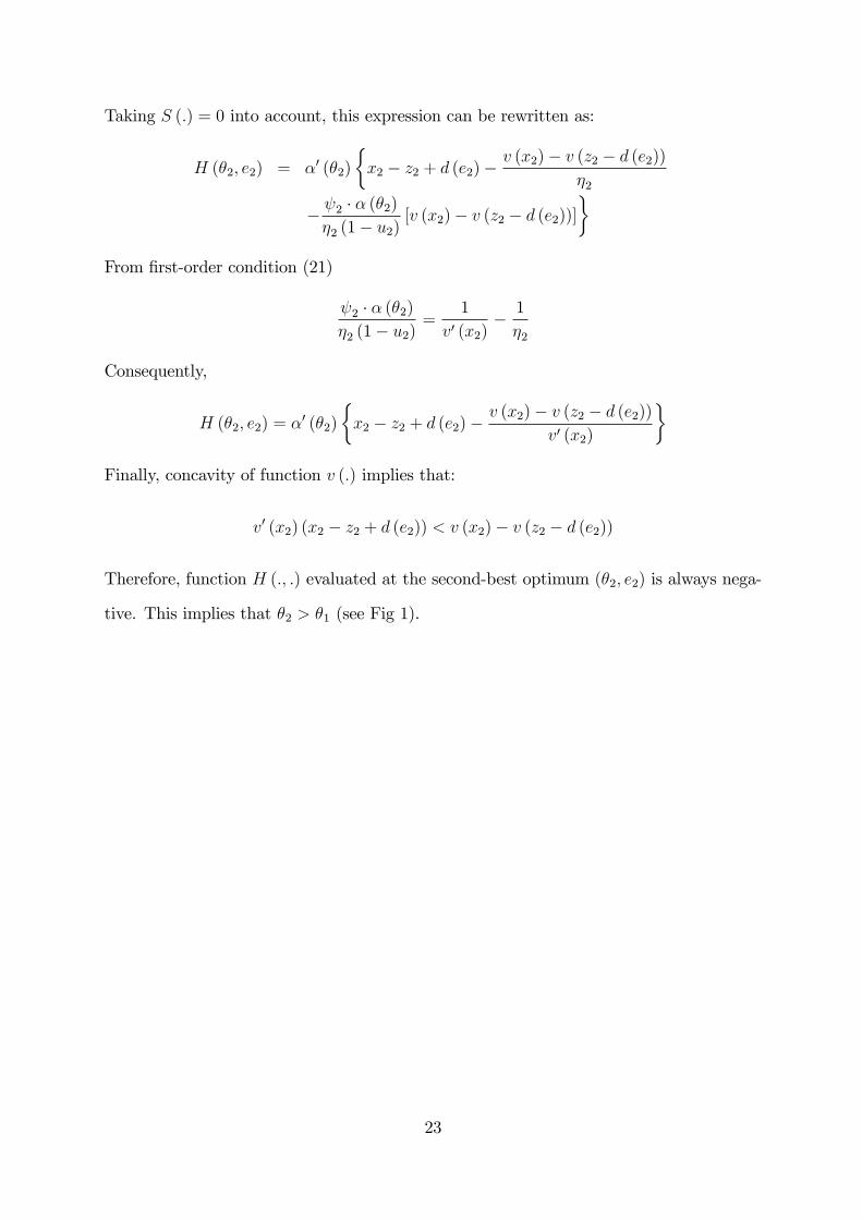
H (�2; e2) = �0 (�2)

�x2 � z2 + d (e2)�

v (x2)� v (z2 � d (e2))

v0 (x2)

�Finally, concavity of function v (:) implies that:

v0 (x2) (x2 � z2 + d (e2)) < v (x2)� v (z2 � d (e2))

Therefore, function H (:; :) evaluated at the second-best optimum (�2; e2) is always nega-

tive. This implies that �2 > �1 (see Fig 1).

23