STATISTICAL RESEARCH REPORT Institute of Mathematics University of Oslo

No 7 1973

ON THE OPTIMAL ALLOCATION OF OBSERVATIONS IN EXPERIMENTS

WITH MIXTURE

by

Petter Laake

Contents

1 • Introduction

2.1 Optimal allocation of observations for the linear polynomial

2.2 Optimal allocation of observations for the quadratic polynomial

2.3 Optimal allocation of observations for the special cubic polynomial

2.4 Optimal allocation of observations for the general cubic polynomial

Definition of the simplex-centroid design

3.1 Optimal allocation of observations for the simplex-centroid design with q = 3

3.2 Optimal allocation of observations for the simplex-centroid design with q = 4

Appendix

References

page

1

3

6

1 1

12

13

14

15

16

17

- 1 -

1. Introduction.

Consider an experiment with mixture, that is an experlinent where

the property studied does not depend on the total amount in the

mixture, but only on the proportions of the factors. The property

studied is called the response.

Denote the i-th factor by xi and suppose that we are

studying a q-component mixture with

x. > 0 1 = 1,2, ••• ,q l. =

x 1 +x2+ ••• +xq=1 ( 1 • 1 )

Hence the experimental design is restricted to the (q-1)-dimen­

tional simplex

q-1 S 1=iCx-1., ••• ,x 11'riJO<L:x.<1, x.>O, i=1,2, ••• ,q-1l q- ~ q..:. .tt -i=1 1.- 1.=

( 1. 2)

Scheffe (1958) introduced the lq,ml-simplex-lattice design where

the values of factor x. l.

x. l.

1 2 = 0 ,-,-, ••• '1 mm

are

i=1,2, ••• ,q

All possible mixtures with these proportions of the factors

are used. The polynomial associated with the simplex-lattice is

q T] = fj + L: fJ . X . + L; p . . X . X . + L: fJ 1.' -; lrXl.. X J' XJr + • • •

• O i=1 l. l. 1<i<"<n l.J l. J 1<i<'<k~ dA ~ - _J_~ - _J_ -~

(1.4)

This polynomial has as many coefficients as there are design­

points in the lq,m}-simplex-lattice design.

- 2 -

Let the estimated polynomial be

...

... where the ~-s are the least-squares estimates. The results

for some given simplex-lattice designs and the associated poly­

nomials can be found in Scheffe (1958), Gor.manand Hinman (1962).

Box and Draper (1959) considered the choice of design on

Sq_1 for fitting a first order polynomial model. They used the

optimality criterion based on minimizing the mean square devi­

ation averaged over the experimental region when the true model

is a polynomi.al of second order. Draper and Lawrence ( 1965a, b)

considered the problem for m=3 and m=4 • Becker (1970) con-

sidered the choice of design for a general m and proved the

generalization of the suggestions made by Box, Draper and

Lawrence.

We are searching for an optimal allocation of the obser­

vations tru{en on the simplex-lattice. Let

1v = J s q-1

be integrated variance over Sq_ 1 • Suppose that total number

of observations equals N • Our optimality criterion is to

choose the number of observations in each designpoint so that

W is minimized.

The fundamental results concerning

section 7 in Scheffe (1958).

('V

var Tt can be found in

- 3 -

2.1. Optimal allocation of observations for the linea£_]£~~£1·

Consider the linear polynomial

1l = q L: ~.x.

. 1 l l l=

and a jq,1l-simplex-lattice. Vie are thus studying the response A

of "pure components". Suppone that 'lli is the observed response

on the lq,1}-simplex-lattice. According to Scheffe (1958)

and

q .... 11 = ~ n.x .

. 1 'l l l=

"' var 11 =

since we assume that the observations are independent with equal

variance Let r. l

be the number of observations on each

lattice-point.

Then

We want to minimize (2.1.1) under the side condition

q L: r. = N

i=1 l

According to (A.1) in Appendix

w = j' var n a.x1 ••• dx _ 1 =cr 2 rt2(+3 )) . f _L = q q l=1 ri

(2 .1 • 1 )

- 4 -

where

Here W is to be minimized under the side condition

q L: r. = N

. 1 J. J.=

Introduce

w q 1 w1 = --2 = a1(q) L: --

cr i==1 ri

w1 is then to be minimized under the given side condition.

This extremum problem can be solved by studying

Thus

~ = a1 (q) f 1- +"A( t r.-N) i=1 ri i=1 J.

-a1(q) r~2 +A J.

q L: r .-N

. 1 J. l=

The extremum value is thus the solution of

Hence

N r. =-J. q i=1,2, ••• ,q

- 5 -

This indicates that, using a linear polynomial, we take equal

number of observations of the response to "pure components".

The result seems intuitively obvious.

If N is a multiple of q, r. J.

is an integer. If If is

not a multiple of q , that is

kq < N < (k+1)q , k an integer,

we choose k observations of the response to each "pure compo­

nent". The remainding N-kq observations can either be distri-

buted randomly on the lattice-points or according to special

interest in the coefficients Pi •

Obviously the solution of the extremum problem gives a

minimum value of vf • Suppose that r 1 ,r2 , ••• ,rq_1 are chosen

sufficiently close to 0 ' ffi1d

Thus

q-1 ==N-L.:r.

. 1 J. J.=

t L i=1 ri

can be made as large as we want. Consequently we can make W

as large as we want at the scm1e time as the side condition

q 2: r. =If

i=1 J.

is full:filled. The extremum point is thus a minimum point.

- 6 -

2.2. Optimal allocation of observations for the guadratig p~l~

nomial.

Consider the polynomial

1l = q L: ~.x.+ L: ~· .x.x.

i=1 l l 1<i<j~ lJ l J (2.2.1)

and a lq,2l-simplex-lattice, which means that the q factors

are given by

q L: x. = 1

. 1 l l=

x. = O,i,1 l

i=1,2, ••• ,q

From this design the coefficients in the polynomial (2.2.1) are

estimated. This is carried out in Scheffe (1958). Suppose that

Yl· l and 1l .. lJ

are the means of the observed responses on the

simplex-lattice. According to Scheffe (1958) the estimated poly-

nomial is

~ q ~ • 1l = E a.T].+ L: a. ·Yl·.

i=1 l l 1<i<j~ lJ lJ

where

a . = x . ( 2x . -1 ) l l l

(2.2.2) a .. = 4x.x. lJ l J

Suppose that the observations are independent with equal vari­

rulce, a2 and the numbers of observations of the response to

"pure components" and mixtures with X. = X. = t l J

rij • We then get

are r. l

8lld

- 7 -

"' 2 q a.2 a .. 2 var n = a ( L -l- + ~ -11-)

i=1 ri i<j rij

The optimality criterion is now to minimize

subject

I rv w = var T1 dx1 ••• dxq_1

sq-1

to the side condition

q ~ r.+ L r .. = N

. 1 ]. '<' J.J J.= ]. J

We consider

I 2 2 1 + a L a .. - dx1 ••• dx 1 '<' J.J r.. q-S J. J J.J q-1

and calculate

a2(q) = I ai2dx1 ••• dxq-1

sq-1

According to (A.1) in Appendix we get

i=1,2, ••• ,q

(2.2.3)

(2.2.4)

- 8 -

b2 (q) = J 16xi2xj 2dx1 ••• dxq_1

sq-1

64 = (3+q)!

i = 1,2, ••• ,q j = 1,1, ••• ,q

i<j

Substituting (2.2.4) and (2.2.5) into (2.2.31 we get

We introduce

w1 = a2(q) £ 1 + b2(q).<~. _1_ i=1 ri l J rij

(2.2.5)

(2.2 .. 6)

and we are interested in minimizing (2.2.6) subject to the side

condition

q ~ r. + ~ r .. == N

i=1 l i<j lJ

~1e problem is solved by differentiating

which yields

()ip q ~ = ~ r. + L: r .. -N OA . 1 l '<' lJ l= l J

(2.2.7)

- 9 -

We then solve the equations

b~ Qqi Qq) -=-=~=0 or. or. . u A

l lJ

and get

(2.2.8)

Substituting (2.2.8) into the side condition we get

i = 1 I 2, I I I 'q

(2.2.9)

i = 1,2, ••• ,q

j = 1,2, ••• ,q i<j

We are thus led to the conclusion of taking the same number of

observations of the responses to each "pure component" and the

same number of observations of the responses to mixtures where

xi = xj = i . The relative proportion of the number of obser­

vations is given by

ri = Ja2(q) i = 1,2, .... ,q r ..

~b2(q) (2.2.10)

lJ j = 1,2, ••• ,q i<j

Using an argun1ent similar to the argument used in section 2.1,

we get that the solution (2.2.9) gives minimum value of W •

- 10 -

Ex. 1: We are interested in studying the relative proportions

of observations, given by (2.2.10) for some values of q •

The result is given in table 1

q ri;rij

3 'l 0,433 I

4 i 0.433 i

5 0.500

6 0.612

7 0.750

8 0.901

9 1.060

10 1. 225

20 I 2.948 I

Table 1

For each value of q we choose

r 1=r2= ••• =rq

Table 1 indicates that if q ~ 8 , r 2. and r .. lJ

according to the optimality criterion, so that

are chosen,

r. < r ..• l lJ

This signifies that ~Arhen there are few components in the mixture,

most of the observations are used to estimate the 11 interaction11

between the factors, When there are many components in the

mixture, most of the observations are used to estimate the "main

effects 11 ,

- 11 -

2.3, Qptimal allocation of observations for the special cubic

polynomial.

Consider the special cubic polynomial

g_ 'r1 = L: ~;x~+ L: ~· .x.x.+ L: 13· .kx.x.xk (2.3.1)

i =1 .... .L 1 ::;i <j :sg_ l. J l. J 1 § <j <k:::g_ l. J l. J

When we have chosen the polynomial, we adopt the {g_,2}-simplex-

lattice argumented by the designpoints corresponding to mixture

with x. = x. = x1 = ~ , i, j ,k = 1, 2, ••• , g_ , i < j <. k • l. J c :;

Scheffe (1958) found that estimated response is given by

rv g_ "" "" ,.. 'r1 = L: b.r].+ L: b. ·'rl· .+ L: bi~k'lliJ'k

i=1 l. l. i<j l.J l.J i<j<k -

and

~ ( 2 g_ 2) b. = zx. 6x. -2x.+1-3 L: x. l. l. l. l. j=1 J

b .. k = 27x . x .x1 l.J l. J <::

The observations are assumed to be independent with equal vari-

ance cr 2 , and ri , rij

vations on ~i , ~ij and

response is

and are the numbers of obser-

The variance of the estimated

var n = £ b. 2 o2 + 2:: b .. 2 o2 + L: b. ·i L i=1 l. ri i<j l.J rij i<j<k l.J rijk

Minimizing

- 12 -

W = J var ~ ax1 ••• dxq-i

sq-1

subject to the side condition

q l:: r. + L: r .. + L: rook= N

i=1 ~ i<j 1 J i<j4c ~J

leads to the following conclusion: Choose r 1. , r. 0 and r 0 ok 1J ~J

so that

and

( ) 16 ( 2 ) b3 q = (5+q)! 16q -144q+392

For details concerning the proof, the reader is referred to

Laake (1973). An application of (2.3.1) will be developed in

section 3.1.

2.4. Optimal allocation of observations for the general cubic

polynomial.

Consider the polJ~omial

q fJ = ~ ~oX 0 + L: ~ 0 .x oX 0 + L: y 0 oX oX 0 (x 0 -x.)

i=1 ~ 1 1<i<j<q 1J 1 J 1~<j~ ~J ~ J 1 J

+ L: B 0 0, x oX .xk 1 <i <.. 0 <k:cr,' 1 J.K 1 J ~ - J _----J,

- 13 -

and adopt the jq,3}-simplex-lattice, Applying the optimality

criterion, we obtain the following conclusion: Choose

and so that

r ... = r ... ~~J ~JJ

i = 1,2, ••• ,q

j = 1,2, ••• ,q

i < j

and

where

( ) 81 ( 2 ) b4 q = (5+q)! q -9q+38

For details the reader is referred to Laake (1973).

3. Definition of the slinplex-centroid design.

Scheffe (1963) has proposed an alternative design on the simplex.

The design is called the simplex-centroid design and is defined

by

q observations of 11pure components"

(~) observations of mixtures of two components with equal

proportions

(~) observations of mixtures of three components with equal

- 14 -

proportions

•

1 observation of the mixture with q components all equal

1 to - • q

Suppose that the response can be expressed by the polynomial

q 11 = L: (3.x.+ L: ~· .x.x.+ ••• +(3 12 x1x 2 ••• x

i=1 1 1 1~<j~ 1J 1 J ••• q q

Estimated response is given by

q A A A

2:: (3.x.+ L: (3 •. x.x.+,.,+(3 12 x 1x2 ••• x i=1 1 1 1~<j~ 1J 1 J ••• q q

A

where the (3-s are least squares estimates. The iq,m)-simplex-

lattice designs differ from the simplex-centroid design in that

for a given q there is a family of alternative {q,ml designs

for m = 1,2, ••• t but there is a single simplex-ce~troid design.

3.1 Optimal allocation of observations for the slinplex-centroid

design with g = 3.

In section 2.3 we considered an optimal allocation of observat­

ions for the special cubic polynomial and for a g~neral q •

Comparing the simplex-lattice design and the associated poly­

nomial in section 2,3 with the simplex-centroid design in section

3, we see that ~1e models are identical for q = 3 • The optimal

allocation of observations for q = 3 is therefore given by

substituting q = 3 in (2.3.1). Hence the conclusion is to

choose aJJ.d so that

- 15 -

i = 1,2,3 j = 1,2,3

i < j

3.2 Optimal allocation o£ observations in the simElex-centroid

design with g = 4.

Consider the polynomial

4 'll = 2.:: ~.x.+ 2.:: ~- .x.x.+ 2.:: p .. kx.x.xl+~1234x1x2x3x4

i=1 ~ ~ 19-<j<4 ~J ~ J 1<i<j<k<4 ~J ~ J t .

and the simplex-centroid design with q = 4. The optimum proce­

dure now leads to the following conclusion: Choose

r., ~

so that

r. :r .. :r .. k:r1234 = 1:1.30:2.10:3.84 ~ ~J ~J

i = 1,2,3,4 j = 1 ,2,3,4 k = 1,2,3,4

i < j < k

For details concerning the proof the reader is referred to

Laake (1973).

- 16 -

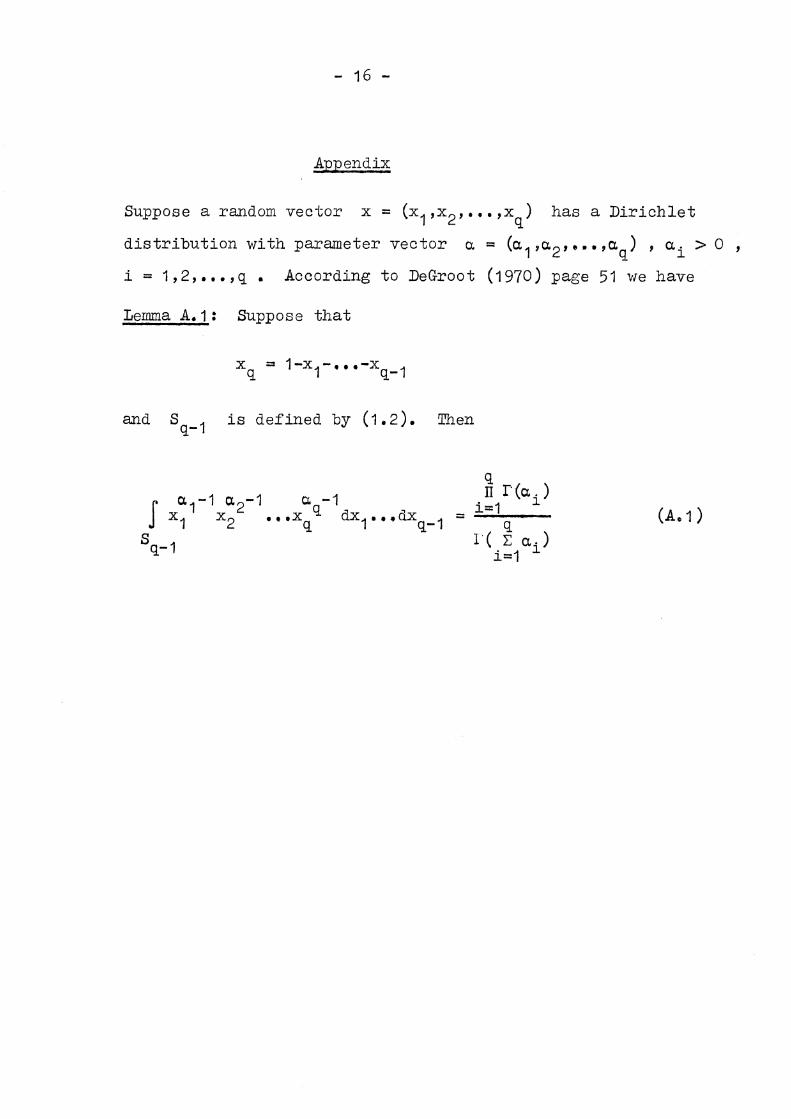
Appendix

Suppose a random vector x = (x1,x2 , ••• ,xq) has a Dirichlet

distribution with parameter vector o. = (a. 1 ,o.2,, •• ,a.q) , a.i > 0 ,

i = 1,2, ••• ,q. According to DeGroot (1970) page 51 we have

Lemma A.1: Suppose that

and s q-1

x = 1-x - ••• -x q 1 q-1

is defined by (1.2). Then

q n r(o..)

. 1 J. J.=

= --------q I( L: o.i)

i=1

(Ao 1)

- 17 -

References

N.G. Becker (1970): Mixture design for a model linear in the proportions. Biometrika, 57, 329-38.

G.E.P. Box and N.R. Draper (1959). A basis for the selection of a response surface design. J. Am. Statis. Ass., 54,

622-54.

M. DeGroot (1970): Optimal statistical decisions. McGraw Hill Book Company.

N.R. Draper and W.L. Lawrence (1965a): Mixture designs for three factors. J. Roy, Statist.Soc., B27, 450-65.

N.R. Draper and W.L. Lawrence ( 1965b): Mixture designs for four factors. J. Roy. Statist.Soc., B27, 473-8

J.W. Gorman and J.E. Hinman (1962): Simplex-lattice-designs for multicomponent systems. Technometrics, 4, 463-88.

P. Laake (1973): Noen optimale egenskaper i eksperimenter med blanding. Hovedoppgave i statistikk. Matematisk insti­tutt, Universitetet i Oslo.

H. Scheffe (1958): Experiments with mixtures. J·. Roy. Statist. Soc., B20, 344-60.

H. Scheffe (1963): The sDnplex-centroid design for experiments with mixtlrres. J. Roy. Statist. Soc., B25, 235-63.