on the modeling and design of zero-net mass flux …

ON THE MODELING AND DESIGN OF ZERO-NET MASS FLUX ACTUATORS

By

QUENTIN GALLAS

A DISSERTATION PRESENTED TO THE GRADUATE SCHOOL OF THE UNIVERSITY OF FLORIDA IN PARTIAL FULFILLMENT

OF THE REQUIREMENTS FOR THE DEGREE OF DOCTOR OF PHILOSOPHY

UNIVERSITY OF FLORIDA

2005

Copyright 2005

by

Quentin Gallas

Pour ma famille et mes amis, d’ici et de là-bas… (To my family and friends, from here and over there…)

iv

ACKNOWLEDGMENTS

Financial support for the research project was provided by a NASA-Langley

Research Center Grant and an AFOSR grant. First, I would like to thank my advisor, Dr.

Louis N. Cattafesta. His continual guidance and support gave me the motivation and

encouragement that made this work possible. I would also like to express my gratitude

especially to Dr. Mark Sheplak, and to the other members of my committee (Dr. Bruce

Carroll, Dr. Bhavani Sankar, and Dr. Toshikazu Nishida) for advising and guiding me

with various aspects of this project. I thank the members of the Interdisciplinary

Microsystems group and of the Mechanical and Aerospace Engineering department

(particularly fellow student Ryan Holman) for their help with my research and their

friendship. I thank everyone who contributed in a small but significant way to this work.

I also thank Dr. Rajat Mittal (George Washington University) and his student Reni Raju,

who greatly helped me with the computational part of this work.

Finally, special thanks go to my family and friends, from the States and from

France, for always encouraging me to pursue my interests and for making that pursuit

possible.

v

TABLE OF CONTENTS page

ACKNOWLEDGMENTS ................................................................................................. iv

LIST OF TABLES............................................................................................................. ix

LIST OF FIGURES ........................................................................................................... xi

LIST OF SYMBOLS AND ABBREVIATIONS ............................................................ xix

ABSTRACT................................................................................................................... xxvi

CHAPTER

1 INTRODUCTION ........................................................................................................1

Motivation.....................................................................................................................1 Overview of a Zero-Net Mass Flux Actuator ...............................................................3 Literature Review .........................................................................................................7

Isolated Zero-Net Mass Flux Devices ...................................................................7 Applications ...................................................................................................8 Modeling approaches ...................................................................................11

Zero-Net Mass Flux Devices with the Addition of Crossflow............................15 Fluid dynamic applications ..........................................................................16 Aeroacoustics applications ...........................................................................18 Modeling approaches ...................................................................................19

Unresolved Technical Issues ...............................................................................25 Objectives ...................................................................................................................27 Approach and Outline of Thesis .................................................................................28

2 DYNAMICS OF ISOLATED ZERO-NET MASS FLUX ACTUATORS ...............30

Characterization and Parameter Definitions...............................................................31 Lumped Element Modeling ........................................................................................34

Summary of Previous Work ................................................................................34 Limitations and Extensions of Existing Model ...................................................38

Dimensional Analysis.................................................................................................44 Definition and Discussion ...................................................................................44 Dimensionless Linear Transfer Function for a Generic Driver...........................46

vi

Modeling Issues ..........................................................................................................51

Cavity Effect........................................................................................................51 Orifice Effect .......................................................................................................52

Lumped element modeling in the time domain............................................52 Loss mechanism ...........................................................................................61

Driving-Transducer Effect...................................................................................63 Test Matrix..................................................................................................................69

3 EXPERIMENTAL SETUP ........................................................................................72

Experimental Setup.....................................................................................................72 Cavity Pressure....................................................................................................75 Diaphragm Deflection .........................................................................................76 Velocity Measurement.........................................................................................79 Data-Acquisition System.....................................................................................82

Data Processing ..........................................................................................................85 Fourier Series Decomposition ....................................................................................92 Flow Visualization......................................................................................................97

4 RESULTS: ORIFICE FLOW PHYSICS....................................................................99

Local Flow Field.......................................................................................................100 Velocity Profile through the Orifice: Numerical Results ..................................100 Exit Velocity Profile: Experimental Results .....................................................109 Jet Formation .....................................................................................................116

Influence of Governing Parameters ..........................................................................118 Empirical Nonlinear Threshold .........................................................................119 Strouhal, Reynolds, and Stokes Numbers versus Pressure Loss .......................121

Nonlinear Mechanisms in a ZNMF Actuator ...........................................................128

5 RESULTS: CAVITY INVESTIGATION................................................................137

Cavity Pressure Field................................................................................................137 Experimental Results.........................................................................................138 Numerical Simulation Results ...........................................................................141

Computational fluid dynamics ...................................................................142 Femlab........................................................................................................147

Compressibility of the Cavity...................................................................................150 LEM-Based Analysis.........................................................................................151 Experimental Results.........................................................................................156

Driver, Cavity, and Orifice Volume Velocities ........................................................162

6 REDUCED-ORDER MODEL OF ISOLATED ZNMF ACTUATOR....................171

Orifice Pressure Drop ...............................................................................................171 Control Volume Analysis ..................................................................................172 Validation through Numerical Results ..............................................................175

vii

Discussion: Orifice Flow Physics......................................................................181 Development of Approximate Scaling Laws ....................................................188

Experimental results ...................................................................................188 Nonlinear pressure loss correlation ............................................................194

Refined Lumped Element Model..............................................................................198 Implementation..................................................................................................198 Comparison with Experimental Data ................................................................202

7 ZERO-NET MASS FLUX ACTUATOR INTERACTING WITH AN EXTERNAL BOUNDARY LAYER .......................................................................211

On the Influence of Grazing Flow............................................................................211 Dimensional Analysis...............................................................................................218 Reduced-Order Models.............................................................................................223

Lumped Element Modeling-Based Semi-Empirical Model of the External Boundary Layer .............................................................................................224

Definition ...................................................................................................224 Boundary layer impedance implementation in Helmholtz resonators .......229 Boundary layer impedance implementation in ZNMF actuator.................238

Velocity Profile Scaling Laws...........................................................................241 Scaling law based on the jet exit velocity profile.......................................244 Scaling law based on the jet exit integral parameters ................................261 Validation and Application ........................................................................270

8 CONCLUSIONS AND FUTURE WORK...............................................................273

Conclusions...............................................................................................................273 Recommendations for Future Research....................................................................276

Need in Extracting Specific Quantities .............................................................276 Proper Orthogonal Decomposition....................................................................277 Boundary Layer Impedance Characterization ...................................................279 MEMS Scale Implementation ...........................................................................280 Design Synthesis Problem.................................................................................282

APPENDIX

A EXAMPLES OF GRAZING FLOW MODELS PAST HELMHOLTZ RESONATORS ........................................................................................................283

B ON THE NATURAL FREQUENCY OF A HELMHOLTZ RESONATOR ..........291

C DERIVATION OF THE ORIFICE IMPEDANCE OF AN OSCILLATING PRESSURE DRIVEN CHANNEL FLOW..............................................................295

D NON-DIMENSIONALIZATION OF A ZNMF ACTUATOR ...............................303

E NON-DIMENSIONALIZATION OF A PIEZOELECTRIC-DRIVEN ZNMF ACTUATOR WITHOUT CROSSFLOW................................................................312

viii

F NUMERICAL METHODOLOGY ..........................................................................326

G EXPERIMENTAL RESULTS: POWER ANALYSIS ............................................331

LIST OF REFERENCES.................................................................................................348

BIOGRAPHICAL SKETCH ...........................................................................................359

ix

LIST OF TABLES

Table page 2-1 Correspondence between synthetic jet parameter definitions...................................34

2-2 Dimensional parameters for circular and rectangular orifices..................................49

2-3 Test matrix for ZNMF actuator in quiescent medium ..............................................69

3-1 ZNMF device characteristic dimensions used in Test 1 ...........................................75

3-2 LDV measurement details.........................................................................................82

3-3 Repeatability in the experimental results..................................................................92

4-1 Ratio of the diffusive to convective time scales .....................................................109

5-1 Cavity volume effect on the device frequency response for Case 1 (Gallas et al.) from the LEM prediction. .......................................................................................153

5-2 Cavity volume effect on the device frequency response for Case 1 (CFDVal) from the LEM prediction. .......................................................................................154

5-3 ZNMF device characteristic dimensions used in Test 2 .........................................156

5-4 Effect of the cavity volume decrease on the ZNMF actuator frequency response for Cases A, B, C, and D.........................................................................................157

7-1 List of configurations used for impedance tube simulations used in Choudhari et al..............................................................................................................................216

7-2 Experimental operating conditions from Hersh and Walker. .................................230

7-3 Experimental operating conditions from Jing et al. ................................................236

7-4 Tests cases from numerical simulations used in the development of the velocity profiles scaling laws................................................................................................242

7-5 Coefficients of the nonlinear least square fits on the decomposed jet velocity profile......................................................................................................................254

x

7-6 Results from the nonlinear regression analysis for the velocity profile based scaling law ..............................................................................................................259

7-7 Results for the parameters a, b and c from the nonlinear system ...........................265

7-8 Integral parameters results ......................................................................................266

7-9 Results from the nonlinear regression analysis for the integral parameters based velocity profile ........................................................................................................267

A-1 Experimental database for grazing flow impedance models ..................................290

B-1 Calculation of Helmholtz resonator frequency. ......................................................293

D-1 Dimensional matrix of parameter variables for the isolated actuator case. ............304

D-2 Dimensional matrix of parameter variables for the general case............................308

E-1 Dimensional matrix of parameter variables............................................................314

G-1 Power in the experimental time data.......................................................................332

xi

LIST OF FIGURES

Figure page 1-1 Schematic of typical zero-net mass flux devices interacting with a boundary

layer, showing three different types of excitation mechanisms. .................................4

1-2 Orifice geometry. ........................................................................................................5

1-3 Helmholtz resonators arrays........................................................................................6

2-1 Equivalent circuit model of a piezoelectric-driven synthetic jet actuator.................35

2-2 Comparison between the lumped element model and experimental frequency response measured using phase-locked LDV for two prototypical synthetic jets. ...37

2-3 Comparison between the lumped element model (—) and experimental frequency response measured using phase-locked LDV ( ) for four prototypical synthetic jets..............................................................................................................41

2-4 Variation in velocity profile vs. S = 1, 12, 20, and 50 for oscillatory pipe flow in a circular duct............................................................................................................42

2-5 Ratio of spatial average velocity to centerline velocity vs. Stokes number for oscillatory pipe flow in a circular duct......................................................................43

2-6 Schematic representation of a generic-driver ZNMF actuator..................................47

2-7 Bode diagram of the second order system given by Eq. 2-20, for different damping ratio. ...........................................................................................................48

2-8 Coordinate system and sign convention definition in a ZNMF actuator. .................53

2-9 Geometry of the piezoelectric-driven ZNMF actuator from Case 1 (CFDVal). ......55

2-10 Geometry of the piston-driven ZNMF actuator from Case 2 (CFDVal). ................55

2-11 Time signals of the jet orifice velocity, pressure across the orifice, and driver displacement during one cycle for Case 1. ...............................................................57

2-12 Time signals of the jet orifice velocity, pressure across the orifice and driver displacement during one cycle for Case 2. ...............................................................58

xii

2-13 Numerical results of the time signals for A) pressure drop and B) velocity perturbation at selected locations along the resonator orifice...................................59

2-14 Schematic of the different flow regions inside a ZNMF actuator orifice. ................62

2-15 Equivalent two-port circuit representation of piezoelectric transduction. ................64

2-16 Speaker-driven ZNMF actuator. ...............................................................................66

2-17 Schematic of a shaker-driven ZNMF actuator, showing the vent channel between the two sealed cavities. ...............................................................................67

2-18 Circuit representation of a shaker-driven ZNMF actuator........................................68

3-1 Schematic of the experimental setup for phase-locked cavity pressure, diaphragm deflection and off-axis, two-component LDV measurements. ...............73

3-2 Exploded view of the modular piezoelectric-driven ZNMF actuator used in the experimental test. ......................................................................................................73

3-3 Schematic (to scale) of the location of the two 1/8” microphones inside the ZNMF actuator cavity...............................................................................................76

3-4 Laser displacement sensor apparatus to measure the diaphragm deflection with sign convention. ........................................................................................................77

3-5 Diaphragm mode shape comparison between linear model and experimental data at three test conditions. ......................................................................................79

3-6 LDV 3-beam optical configuration. ..........................................................................80

3-7 Flow chart of measurement setup. ............................................................................83

3-8 Phase-locked signals acquired from the DSA card, showing the normalized trigger signal, displacement signal, pressure signals and excitation signal. .............84

3-9 Percentage error in Error! Objects cannot be created from editing field codes. from simulated LDV data at different signal to noise ratio, using 8192 samples.....87

3-10 Phase-locked velocity profiles and corresponding volume flow rate acquired with LDV for Case 14...............................................................................................89

3-11 Noise floor in the microphone measurements compared with Case 52. ...................91

3-12 Normalized quantities vs. phase angle. .....................................................................93

3-13 Power spectrum of the two pressure recorded and the diaphragm displacement. ...95

3-14 Schematic of the flow visualization setup.................................................................97

xiii

4-1 Numerical results of the orifice flow pattern showing axial and longitudinal velocities, azimuthal vorticity contours, and instantaneous streamlines at the time of maximum expulsion. ..................................................................................101

4-2 Velocity profile at different locations inside the orifice for Case 1........................103



4-5 Vertical velocity contours inside the orifice during the time of maximum expulsion. ................................................................................................................107

4-6 Experimental vertical velocity profiles across the orifice for a ZNMF actuator in quiescent medium at different instant in time for Case 71. ....................................110




4-10 Experimental results of the ratio between the time- and spatial-averaged velocity and time-averaged centerline velocity. .....................................................116

4-11 Experimental results on the jet formation criterion. ...............................................118

4-12 Averaged jet velocity vs. pressure fluctuation for different Stokes number...........120

4-13 Pressure fluctuation normalized by the dynamic pressure based on averaged velocity vs. St h d⋅ ..................................................................................................122

4-14 Pressure fluctuation normalized by the dynamic pressure based on averaged velocity vs. Strouhal number. .................................................................................123

4-15 Vorticity contours during the maximum expulsion portion of the cycle from numerical simulations. ............................................................................................124

4-16 Pressure fluctuation normalized by the dynamic pressure based on ingestion time averaged velocity vs. St h d⋅ . ........................................................................125

4-17 Vorticity contours during the maximum ingestion portion of the cycle from numerical simulations. ............................................................................................126

4-18 Comparison between Case 1 vertical velocity profiles at the orifice ends. ............127

xiv



4-21 Determination of the validity of the small-signal assumption in a closed cavity. ..131

4-22 Log-log plot of the cavity pressure total harmonic distortion in the experimental time signals. ............................................................................................................132

4-23 Log-log plot of the total harmonic distortion in the experimental time signals vs. Strouhal number as a function of Stokes number. ..................................................134

5-1 Coherent power spectrum of the pressure signal for Cases 9 to 20. .......................138

5-2 Phase plot of the normalized pressures taken by microphone 1 versus microphone 2...........................................................................................................139

5-3 Pressure signals experimentally recorded by microphone 1 and microphone 2 as a function of phase in Case 59. ...............................................................................140

5-4 Ratio of microphone amplitude (Pa) vs. the inverse of the Strouhal number, for different Stokes number. .........................................................................................141

5-5 Pressure contours in the cavity and orifice (Case 2) from numerical simulations..143

5-6 Pressure contours in the cavity and orifice (Case 3) from numerical simulations..144

5-7 Cavity pressure probe locations in a ZNMF actuator from numerical simulations. .............................................................................................................145

5-8 Normalized pressure inside the cavity during one cycle at 15 different probe locations from numerical simulation results. ..........................................................146

5-9 Cavity pressure normalized by 2

jVρ vs. phase from numerical simulations corresponding to the experimental probing locations. ............................................147

5-10 Contours of pressure phase inside the cavity by numerically solving the 3D wave equation using FEMLAB...............................................................................148

5-11 Cavity pressure vs. phase by solving the 3D wave equation using FEMLAB and corresponding to the experimental probing locations. ............................................149

5-12 Log-log frequency response plot of Case 1 (Gallas et al.) as the cavity volume is decreased from the LEM prediction........................................................................153

5-13 Log-log frequency response plot of Case 1 (CFDVal) as the cavity volume is decreased from the LEM prediction........................................................................154

xv

5-14 Experimental log-log frequency response plot of a ZNMF actuator as the cavity volume is decreased for a constant input voltage. ..................................................158

5-15 Close-up view of the peak locations in the experimental actuator frequency response as the cavity volume is decreased for a constant input voltage. ..............158

5-16 Normalized quantities vs. phase of the jet volume rate, cavity pressure and centerline driver velocity.. ......................................................................................160

5-17 Experimental results of the ratio of the driver to the jet volume velocity function of dimensionless frequency as the cavity volume decreases. .................................164

5-18 Experimental jet to driver volume flow rate versus actuation to Helmholtz frequency.................................................................................................................166

5-19 Current divider representation of a piezoelectric-driven ZNMF actuator. .............168

5-20 Frequency response of the power conservation in a ZNMF actuator from the lumped element model circuit representation for Case 1 (Gallas et al.) .................169

6-1 Control volume for an unsteady laminar incompressible flow in a circular orifice, from y/h = -1 to y/h = 0...............................................................................172

6-2 Numerical results for the contribution of each term in the integral momentum equation as a function of phase angle during a cycle..............................................176

6-3 Definition of the approximation of the orifice entrance velocity from the orifice exit velocity.............................................................................................................178

6-4 Momentum integral of the exit and inlet velocities normalized by Error! Objects cannot be created from editing field codes. and comparing with the actual and approximated entrance velocity. .............................................................................179

6-5 Total momentum integral equation during one cycle, showing the results using the actual and approximated entrance velocity. ......................................................181

6-6 Numerical results of the total shear stress term versus corresponding lumped linear resistance during one cycle. ..........................................................................183

6-7 Numerical results of the unsteady term versus corresponding lumped linear reactance during one cycle. .....................................................................................184

6-8 Numerical results of the normalized terms in the integral momentum equation as a function of phase angle during a cycle. ...........................................................187

6-9 Comparison between lumped elements from the orifice impedance and analytical terms from the control volume analysis. ................................................188

xvi

6-10 Experimental results of the orifice pressure drop normalized by the dynamic pressure based on averaged velocity versus St h d⋅ for different Stokes numbers. ..................................................................................................................191

6-11 Experimental results of each term contributing in the orifice pressure drop coefficient vs. St h d⋅ . ............................................................................................192

6-12 Experimental results of the relative magnitude of each term contributing in the orifice pressure drop coefficient vs. intermediate to low St h d⋅ . .........................193

6-13 Experimental results for the nonlinear pressure loss coefficient for different Stokes number and orifice aspect ratio. ..................................................................196

6-14 Nonlinear term of the pressure loss across the orifice as a function of St h d⋅ from experimental data. ..........................................................................................197

6-15 Implementation of the refined LEM technique to compute the jet exit velocity frequency response of an isolated ZNMF actuator. ................................................201

6-16 Comparison between the experimental data and the prediction of the refined and previous LEM of the impulse response of the jet exit centerline velocity. Actuator design corresponds to Case I from Gallas et al. .......................................203

6-17 Comparison between the experimental data and the prediction of the refined and previous LEM of the impulse response of the jet exit centerline velocity. Actuator design corresponds to Case II from Gallas et al.......................................205

6-18 Comparison between the experimental data and the prediction of the refined and previous LEM of the impulse response of the jet exit centerline velocity. Actuator design is from Gallas and is similar to Cases 41 to 50. ...........................207

6-19 Comparison between the refined LEM prediction and experimental data of the time signals of the jet volume flow rate..................................................................209

7-1 Spanwise vorticity plots for three cases where the jet Reynolds number Re is increased..................................................................................................................212

7-2 Spanwise vorticity plots for three cases where the boundary layer Reynolds number is increased. ...............................................................................................213

7-3 Comparison of the jet exit velocity profile with increasing....................................214

7-4 Pressure contours and streamlines for mean A) inflow, and B) outflow through a resonator in the presence of grazing flow. ..............................................................218

7-5 LEM equivalent circuit representation of a generic ZNMF device interacting with a grazing boundary layer.................................................................................224

xvii

7-6 Schematic of an effort divider diagram for a Helmholtz resonator. .......................230

7-7 Comparison between BL impedance model and experiments from Hersh and Walker as a function of Mach number for different SPL. ......................................233

7-8 Experimental setup used in Jing et al......................................................................236

7-9 Comparison between model and experiments from Jing et al. ...............................237

7-10 Effect of the freestream Mach number on the frequency response of the ZNMF design from Case 1 (CFDVal) using the refined LEM. ..........................................239

7-11 Effect of the freestream Mach number on the frequency response of the ZNMF design from Case 1 (Gallas et al.) ...........................................................................240

7-12 Schematic of the two approaches used to develop the scaling laws from the jet exit velocity profile. ................................................................................................244

7-13 Methodology for the development of the velocity profile based scaling law. ........245

7-14 Nonlinear least square curve fit on the decomposed jet velocity profile for Case I. ..............................................................................................................................247

7-15 Nonlinear least square curve fit on the decomposed jet velocity profile for Case III.............................................................................................................................248

7-16 Nonlinear least square curve fit on the decomposed jet velocity profile for Case V..............................................................................................................................249

7-17 Nonlinear least square curve fit on the decomposed jet velocity profile for Case VII. ..........................................................................................................................250

7-18 Nonlinear least square curve fit on the decomposed jet velocity profile for Case IX. ...........................................................................................................................251

7-19 Nonlinear least square curve fit on the decomposed jet velocity profile for Case XI. ...........................................................................................................................252

7-20 Nonlinear least square curve fit on the decomposed jet velocity profile for Case XIII..........................................................................................................................253

7-21 Comparison between CFD velocity profile, decomposed jet velocity profile, and modeled velocity profile, at the orifice exit, for four phase angles during a cycle. .......................................................................................................................255

7-22 Test case comparison between CFD data and the scaling law based on the velocity profile at four phase angles during a cycle................................................260

7-23 Methodology for the development of the integral parameters based scaling law...262

xviii

7-24 Comparison between the results of the integral parameters from the scaling law and the CFD data for the test case...........................................................................268

7-25 Example of a practical application of the ZNMF actuator reduced-order model in a numerical simulation of flow past a flat plate. .................................................271

8-1 POD analysis applied on numerical data for ZNMF actuator with a grazing BL...278

8-2 Use of quarter-wavelength open tube to provide an infinite impedance. ..............280

8-3 Representative MEMS ZNMF actuator. .................................................................281

8-4 Predicted output of MEMS ZNMF actuator. ..........................................................281

A-1 Acoustic test duct and siren showing a liner panel test configuration. ...................285

A-2 Schematic of test apparatus used in Hersh and Walker. .........................................286

A-3 Apparatus for the measurement of the acoustic impedance of a perforate used by Kirby and Cummings. ........................................................................................288

A-4 Sketch of NASA Grazing Impedance Tube. ...........................................................290

B-1 Helmholtz resonator. ...............................................................................................291

C-1 Rectangular slot geometry and coordinate axis definition......................................295

D-1 Orifice details with coordinate system....................................................................303

F-1 Schematic of A) the sharp-interface method on a fixed Cartesian mesh, and B) the ZNMF actuator interacting with a grazing flow. ..............................................328

F-2 Typical mesh used for the computations. A) 2D simulation. B) 3D simulation...329

F-3 Example of 2D and 3D numerical results of ZNMF interacting with a grazing boundary layer.........................................................................................................329

xix

LIST OF SYMBOLS AND ABBREVIATIONS

0c isentropic air speed of sound [m/s]

aCC cavity acoustic compliance = 20c∀ ρ [s2.m4/kg]

aDC diaphragm short-circuit acoustic compliance =0acV

P=

∆∀ [s2.m4/kg]

DC orifice discharge coefficient [1]

fC skin friction coefficient = 2

0.5w jVτ ρ [1]

Cµ momentum coefficient during the time of discharge [1]

12

nCφ successive moments of jet velocity profile [1]

d orifice diameter [m]

Hd hydraulic diameter = ( ) ( )4 area wetted perimeter [m]

D orifice entrance diameter (facing the cavity) [m]

cD cavity diameter (for cylindrical cavities) [m]

f actuation frequency [Hz]

df driver natural frequency [Hz]

Hf Helmholtz frequency = ( ) 01 2 nc S hπ ′∀ = ( )( )1 2 aN aRad aCM M Cπ + [Hz]

nf natural frequency of the uncontrolled flow [Hz]

0f fundamental frequency [Hz]

1f , 2f synthetic jet lowest and highest resonant frequencies, respectively [Hz]

xx

h orifice height [m]

h′ effective length of the orifice = 0h h+ [m]

0h “end correction” of the orifice = 0.96 nS [m]

H cavity depth (m) / boundary layer shape factor = θ δ ∗ [1]

0I impulse per unit length [1]

k wave number = 0cω [m-1]

dK nondimensional orifice loss coefficient [1]

0L stroke length [m]

aDM diaphragm acoustic mass = ( )2 2

2 0

2 R

A w r rdrπ ρ ⎡ ⎤⎣ ⎦∆∀ ∫ [kg/m4]

aNM orifice acoustic mass due to inertia effect [kg/m4]

aOM orifice acoustic mass = aN aRadM M+ [kg/m4]

aRadM orifice acoustic radiation mass [kg/m4]

p′ acoustic pressure [Pa]

P differential pressure on the diaphragm [Pa]

iP incident pressure [Pa]

Pw Power [W]

q′ acoustic particle volume velocity [m3/s]

cQ volume flow rate through the cavity = j dQ Q− [m3/s]

dQ volume flow rate displaced by the driver = jω∆∀ [m3/s]

jQ volume flow rate through the orifice [m3/s]

xxi

jQ time averaged orifice volume flow rate during the expulsion stroke [m3/s]

r radial coordinate in cylindrical coordinate system [m]

R radius of curvature of the surface [m]

aDR diaphragm acoustic resistance = 2 aD aDM Cζ [kg/m4.s]

aNR viscous orifice acoustic resistance [kg/m4.s]

aOlinR linear orifice acoustic resistance = aNR [kg/m4.s]

aOnlR nonlinear orifice acoustic resistance [kg/m4.s]

0R specific resistance [kg/m2.s]

Re jet Reynolds number = jV d ν [1]

s Laplace variable = jω [rad/s]

S Stokes number = 2dω ν [1]

St jet Strouhal number = jd Vω [1]

cS cavity cross sectional area [m2]

dS driver cross sectional area [m2]

nS orifice neck area [m2]

u′ acoustic particle velocity [m/s]

bu bias flow velocity through the orifice [m/s]

u∗ wall friction velocity [m/s]

U∞ freestream mean velocity [m/s]

CLv centerline orifice velocity [m/s]

xxii

jV spatial averaged jet exit velocity = j nQ S = ( )2 jVπ [m/s]

jV spatial and time-averaged jet exit velocity during the expulsion stroke [m/s]

acV input ac voltage [V]

jV normalized jet velocity = jv U∞ [m/s]

w length of a rectangular orifice [m]

( )w r transverse displacement of the diaphragm [m]

W width of the cavity [m]

0W centerline amplitude of the driver [m]

aX acoustic reactance = aMω [kg/m4.s]

0X specific reactance [kg/m2.s]

12X φ skewness of jet velocity profile [1]

dy vibrating driver displacement [m]

jy fluid particle displacement at the orifice [m]

aZ acoustic impedance = a aR jX+ = p q′ ′ [kg/m4.s2]

aCZ acoustic cavity impedance = ( ) 1aCj Cω − = ( )c d jP Q Q∆ − [kg/m4.s2]

aOZ acoustic impedance of the orifice = aOlin aOnl aOR R j Mω+ + = c jP Q∆ [kg/m4.s2]

aBLZ acoustic impedance of the grazing boundary layer = aBL aBLR jX+ [kg/m4.s2]

,aO tZ total acoustic impedance of the orifice = aO aBLZ Z+ [kg/m4.s2]

0Z specific impedance = 0 0R jX+ = p u′ ′ [kg/m2.s2]

0, pZ perforate specific impedance = 0, 0,p pR jX+ = 0Z σ [kg/m2.s2]

xxiii

α thermal diffusivity [m2/s]

β nondimensional pressure gradient = ( )( )w dP dxδ τ∗ [1]

χ normalized reactance [1]

δ boundary layer thickness [m]

δ ∗ boundary layer displacement thickness [m]

Stokesδ Stokes layer thickness = ν ω [m]

pc∆ normalized pressure drop = ( ) ( )2

0 0.5y jp p Vρ− [1]

cP∆ cavity pressure [Pa]

∆∀ volume displaced by the driver [m3]

aφ electroacoustic turns ratio of the piezoceramic diaphragm = a aDd C [Pa/ V]

icφ phase difference between the incident sound field and the cavity sound field [deg]

γ ratio of the specific heats [1]

λ wavelength = 0 2c f k= π [m]

µ dynamic viscosity = ρν [kg/m.s]

ν cinematic viscosity [m2/s]

ρ density [kg/m3]

Aρ area density [kg/m2]

θ boundary layer momentum thickness [m] / normalized resistance [1]

σ porosity of the perforate plate = ( )hole area total areaholesN × [%]

σ ratio of the orifice to cavity cross sectional area = n cS S [1]

wτ wall shear stress [kg/m.s2]

xxiv

∀ cavity volume [mm3]

ω radian frequency = 2 fπ [rad/s]

vΩ vorticity flux [m2/s]

ζ damping coefficient [1] / normalized impedance = jθ χ+ [1]

pζ normalized impedance of a perforate = p pjθ χ+ [1]

C compliance ratio = aD aCC C [1]

M mass ratio = aD aOM M [1]

R resistance ratio = aN aDR R [1]

Commonly used subscripts:

a acoustic domain

c cavity

CL centerline

d driver

D diaphragm

ex expulsion phase of the cycle

in injection phase of the cycle

j jet

lin linear

nl nonlinear

p perforate

0 specific

∞ freestream

xxv

Commonly used superscripts:

spatial averaged

spatial and time averaged

’ fluctuating quantity

Abbreviations:

BL Boundary Layer

CFD Computational Fluid Dynamics

HWA Hot Wire Anemometry

LDV Laser Doppler Velocimetry

LEM Lumped Element Modeling

MEMS Micro Electromechanical Systems

MSV Mean Square Value

PIV Particle Image Velocimetry

POD Proper Orthogonal Decomposition

RMS Root Mean Square

ZNMF Zero-Net Mass Flux

Throughout this dissertation, the term synthetic jet actuator has the same meaning

as zero-net mass flux actuator, although the former is physically more restricting to

specific applications (strictly speaking, a jet must be formed). Similarly, the terms

grazing flow and bias flow in the acoustic community are used interchangeably with the

respective fluid dynamics terminology crossflow and mean flow, since they refer to the

same phenomenon.

xxvi

Abstract of Dissertation Presented to the Graduate School of the University of Florida in Partial Fulfillment of the Requirements for the Degree of Doctor of Philosophy

ON THE MODELING AND DESIGN OF ZERO-NET MASS FLUX ACTUATORS

By

Quentin Gallas

May 2005

Chair: Louis Cattafesta Major Department: Mechanical and Aerospace Engineering

This dissertation discusses the fundamental dynamics of zero-net mass flux

(ZNMF) actuators commonly used in active flow-control applications. The present work

addresses unresolved technical issues by providing a clear physical understanding of how

these devices behave in a quiescent medium and interact with an external boundary layer

by developing and validating reduced-order models. The results are expected to

ultimately aid in the analysis and development of design tools for ZNMF actuators in

flow-control applications.

The case of an isolated ZNMF actuator is first documented. A dimensional

analysis identifies the key governing parameters of such a device, and a rigorous

investigation of the device physics is conducted based on various theoretical analyses,

phase-locked measurements of orifice velocity, diaphragm displacement, and cavity

pressure fluctuations, and available numerical simulations. The symmetric, sharp orifice

exit velocity profile is shown to be primarily a function of the Strouhal and Reynolds

numbers and orifice aspect ratio. The equivalence between Strouhal number and

xxvii

dimensionless stoke length is also demonstrated. A criterion is developed and validated,

namely that the actuation-to-Helmholtz frequency ratio is less than 0.5, for the flow in the

actuator cavity to be approximately incompressible. An improved lumped element

modeling technique developed from the available data is developed and is in reasonable

agreement with experimental results.

Next, the case in which a ZNMF actuator interacts with an external grazing

boundary layer is examined. Again, dimensional analysis is used to identify the

dimensionless parameters, and the interaction mechanisms are discussed in detail for

different applications. An acoustic impedance model (based on the NASA “ZKTL

model”) of the grazing flow influence is then obtained from a critical survey of previous

work and implemented in the lumped element model. Two scaling laws are then

developed to model the jet velocity profile resulting from the interaction - the profiles are

predicted as a function of local actuator and flow condition and can serve as approximate

boundary conditions for numerical simulations. Finally, extensive discussion is provided

to guide future modeling efforts.

1

CHAPTER 1

INTRODUCTION

Motivation

The past decade has seen numerous studies concerning an exciting type of active

flow control actuator. Zero-net mass flux (ZNMF) devices, also known as synthetic jets,

have emerged as versatile actuators with potential applications such as thrust vectoring of

jets (Smith and Glezer 1997), heat transfer augmentation (Campbell et al. 1998; Guarino

and Manno 2001), active control of separation for low Mach and Reynolds numbers

(Wygnanski 1997; Smith et al. 1998; Amitay et al. 1999; Crook et al. 1999; Holman et al.

2003) or transonic Mach numbers and moderate Reynolds numbers (Seifert and Pack

1999, 2000a), and drag reduction in turbulent boundary layers (Rathnasingham and

Breuer 1997; Lee and Goldstein 2001). This versatility is primarily due to several

reasons. First, these devices provide unsteady forcing, which has proven to be more

effective than its steady counterpart (Seifert et al. 1993).

Second, since the jet is synthesized from the working fluid, complex fluid circuits

are not required. Finally the actuation frequency and waveform can usually be

customized for a particular flow configuration. Synthetic jets exhausting into a quiescent

medium have been studied extensively both experimentally and numerically.

Additionally, other studies have focused on the interaction with an external boundary

layer for the diverse applications mentioned above. However, many questions remain

unanswered regarding the fundamental physics that govern such complex devices.

2

Practically, because of the presence of rich flow physics and multiple flow

mechanisms, proper implementation of these actuators in realistic applications requires

design tools. In turn, simple design tools benefit significantly from low-order dynamical

models. However, no suitable models or design tools exist because of insufficient

understanding as to how the performance of ZNMF actuator devices scales with the

governing nondimensional parameters. Numerous parametric studies provide a glimpse

of how the performance characteristics of ZNMF actuators and their control effectiveness

depend on a number of geometrical, structural, and flow parameters (Rathnasingham and

Breuer 1997; Crook and Wood 2001; He et al. 2001; Gallas et al. 2003a). However,

nondimensional scaling laws are required since they form an essential component in the

design and deployment of ZNMF actuators in practical flow control applications.

For instance, scaling laws are expected to play an important role in the

aerodynamic design of wings that, in the future, may use ZNMF devices for separation

control. The current design paradigm in the aerospace industry relies heavily on steady

Reynolds Averaged Navier Stokes (RANS) computations. A validated unsteady RANS

(URANS) design tool is required for separation control applications at transonic Mach

numbers and flight Reynolds number. However, these computations can be quite

expensive and time-consuming. Direct modeling of ZNMF devices in these

computations is expected to considerably increase this expense, since the simulations

must resolve the flow details in the vicinity of the actuator while also capturing the global

flow characteristics. A viable alternative to minimize this cost is to simply model the

effect of the ZNMF device as a time- and flow-dependant boundary condition in the

URANS calculation. Such an approach requires that the device be characterized by a

3

small set of nondimensional parameters, and the behavior of the actuator must be well

understood over a wide range of conditions.

Furthermore, successful implementation of robust closed-loop control

methodologies for this class of actuators calls for simple (yet effective) mathematical

models, thereby emphasizing the need to develop a reduced-order model of the flow.

Such low-order models will clearly aid in the analysis and development of design tools

for sizing, design and deployment of these actuators. Below, an overview of the basic

operating principles of a ZNMF actuator is provided.

Overview of a Zero-Net Mass Flux Actuator

Typically, ZNMF devices are used to inject unsteady disturbances into a shear

flow, which is known to be a useful tool for active flow control. Most flow control

techniques require a fluid source or sink, such as steady or pulsed suction (or blowing),

vortex-generator jets (Sondergaard et al. 2002; Eldredge and Bons 2004), etc., which

introduces additional constraints in the design of the actuator and sometimes results in

complicated hardware. This motivates the development of ZNMF actuators, which

introduce flow perturbations with zero-net mass injection, the large coherent structures

being synthesized from the surrounding working fluid (hence the name “synthetic jet”).

A typical ZNMF device with different transducers is shown in Figure 1-1. In

general, a ZNMF actuator contains three components: an oscillatory driver (examples of

which are discussed below), a cavity, and an orifice or slot. The oscillating driver

compresses and expands the fluid in the cavity by altering the cavity volume ∀ at the

excitation frequency f to create pressure oscillations. As the cavity volume is

decreased, the fluid is compressed in the cavity and expels some fluid through the orifice.

4

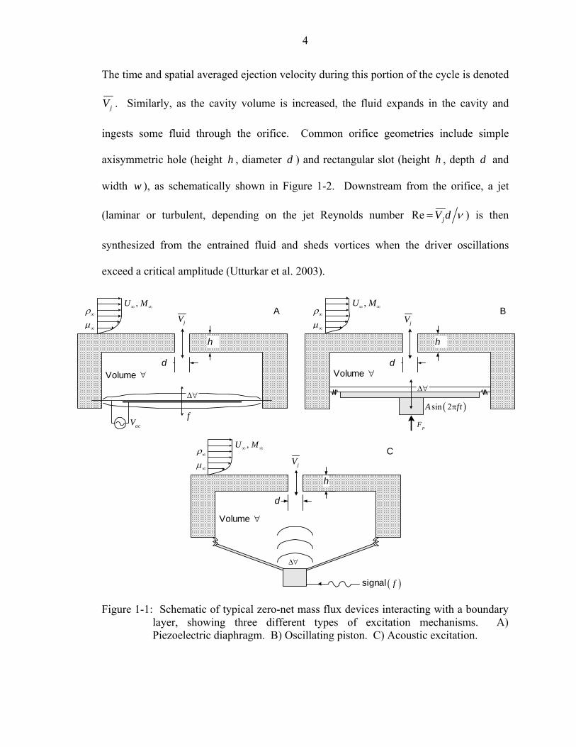
The time and spatial averaged ejection velocity during this portion of the cycle is denoted

jV . Similarly, as the cavity volume is increased, the fluid expands in the cavity and

ingests some fluid through the orifice. Common orifice geometries include simple

axisymmetric hole (height h , diameter d ) and rectangular slot (height h , depth d and

width w ), as schematically shown in Figure 1-2. Downstream from the orifice, a jet

(laminar or turbulent, depending on the jet Reynolds number Re jV d ν= ) is then

synthesized from the entrained fluid and sheds vortices when the driver oscillations

exceed a critical amplitude (Utturkar et al. 2003).

d

h

d

h

( )sin 2A ftπ

pFacV

A B,U M∞ ∞,U M∞ ∞

∞

∞

ρµ

∞

∞

ρµ

d

h

C,U M∞ ∞

∞

∞

ρµ

( )f

∆∀∆∀

∆∀

jV

f

signal

jVjV

Volume ∀ Volume ∀

Volume ∀

Figure 1-1: Schematic of typical zero-net mass flux devices interacting with a boundary

layer, showing three different types of excitation mechanisms. A) Piezoelectric diaphragm. B) Oscillating piston. C) Acoustic excitation.

5

Even though no net mass is injected into the embedded flow during a cycle, a

non-zero transfer of momentum is established with the surrounding flow. The exterior

flow, if present, usually consists of a turbulent boundary layer (since most practical

applications deal with such a turbulent flow) and is characterized by the freestream

velocity U∞ and acoustic speed c∞ , pressure gradient dP dx , radius of curvature R ,

thermal diffusivity α∞ , and displacement δ ∗ and momentum θ thicknesses. Finally, the

ambient fluid is characterized by its density ρ∞ and dynamic viscosity µ∞ .

h

x

y

z

d d h

L

zx

yA B

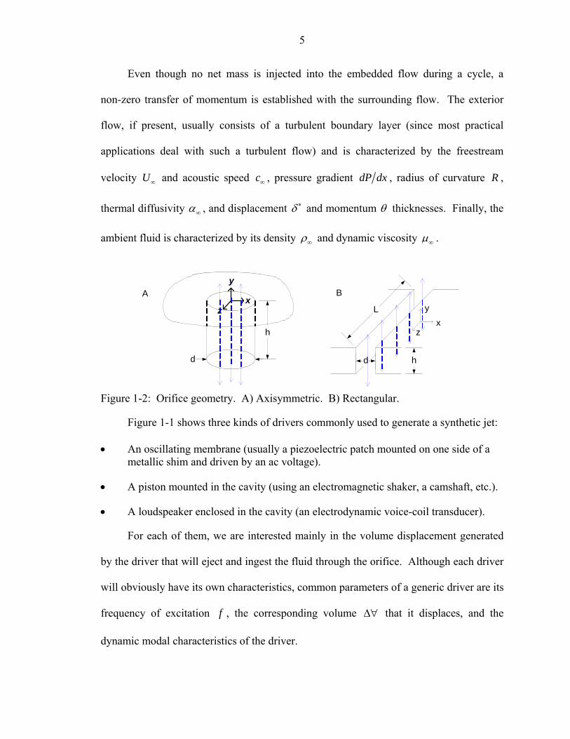
Figure 1-2: Orifice geometry. A) Axisymmetric. B) Rectangular.

Figure 1-1 shows three kinds of drivers commonly used to generate a synthetic jet:

• An oscillating membrane (usually a piezoelectric patch mounted on one side of a metallic shim and driven by an ac voltage).

• A piston mounted in the cavity (using an electromagnetic shaker, a camshaft, etc.).

• A loudspeaker enclosed in the cavity (an electrodynamic voice-coil transducer).

For each of them, we are interested mainly in the volume displacement generated

by the driver that will eject and ingest the fluid through the orifice. Although each driver

will obviously have its own characteristics, common parameters of a generic driver are its

frequency of excitation f , the corresponding volume ∆∀ that it displaces, and the

dynamic modal characteristics of the driver.

6

Figure 1-3: Helmholtz resonators arrays. A) Schematic. B) Application in engine nacelle acoustic liners.

Although noticeable differences exist, it is worthwhile to compare synthetic jets

with the phenomenon of acoustic flow generation, the acoustic streaming, extensively

studied by aeroacousticians in the past (e.g., Lighthill 1978). Acoustic streaming is the

result of a steady flow produced by an acoustic field and is the evidence of the generation

of vorticity by the sound, which occurs for example when sound impinges on solid

boundaries. Quoting Howe (1998, p. 410),

When a sound wave impinges on a solid surface in the absence of mean flow, the dissipated energy is usually converted directly into heat through viscous action. At very high acoustic amplitudes, however, free vorticity may still be formed at edges, and dissipation may take place, as in the presence of mean flow, by the generation of vortical kinetic energy which escapes from the interaction zone by self-induction. This nonlinear mechanism can be important in small perforates or apertures.

This type of flow generation could be relevant in the application of ZNMF devices

where similar nonlinear flow through the orifice is expected. In particular, ZNMF

devices are similar to flow-induced resonators, such as Helmholtz resonators used in

acoustic liners as sound-absorber devices. As Figure 1-3 shows, a simple single degree-

of-freedom (SDOF) liner consists of a perforate sheet backed with honeycomb cavities

and interacting with a grazing flow. Similar liners with a second cavity (or more) are

commonly used in engine nacelles to attenuate the sound noise level. More recently,

Porous face sheet

Honeycomb core Backing sheet

A Acoustic Liners

Inlet

FanNacelle

Exhaust

B

7

Flynn et al. (1990) and Urzynicok and Fernholz (2002) used Helmholtz resonators for

flow control applications. More details will be given in subsequent sections.

Now that an overview of the problem has been presented along with a general

description of a ZNMF device, an in-depth literature survey is given to familiarize the

reader with the existing developments on these subjects and to clearly set the scope of the

current investigation. The objectives of this research are then formulated and the

technical approach described to reach these goals.

Literature Review

This section presents an overview of the relevant research found in the open

literature. The goal is to highlight and extract the principal features of the actuator and

associated fluid dynamics, and to identify unresolved issues. First, the simpler yet

practically significant case in which the synthetic jet exhausts into a quiescent medium is

carefully reviewed. The case in which the synthetic jet interacts with a grazing boundary

layer or crossflow is considered next. The survey reveals available experimental and

numerical simulation data on the local interaction of a ZNMF device with an external

boundary layer. In each subsection, the diverse applications that have employed a ZNMF

actuator are first reviewed, as well as the different modeling approaches used. In the case

of the presence of a grazing boundary layer, examples of applications in the field of fluid

dynamics and aeroacoustics are presented where a parallel with sound absorber

technology is drawn.

Isolated Zero-Net Mass Flux Devices

Numerous studies have addressed the fundamentals and applications of isolated

ZNMF actuators. The list presented next is by no means exhaustive but reflects the major

points and contributions to the understanding of such devices.

8

Applications

Mixing enhancement, heat transfer, or thrust vectoring are the major applications of

isolated ZNMF devices, as opposed to active flow control applications when the actuator

is interacting with an external boundary layer that will be seen in the next section.

Chen et al. (1999) demonstrated the use of ZNMF actuators to enhance mixing in a

gas turbine combustor. They used two streams of hot and cold gas to simulate the mixing

and they measured the temperature distribution downstream of the synthetic jet to

determine the effectiveness of the mixing. Their experiments showed that ZNMF devices

could improve mixing in a turbine jet engine without using additional cold dilution air.

Similarly, modification and control of small-scale motions and mixing processes

via ZNMF actuators were investigated by Davis et al. (1999). Their experiments used an

array of ZNMF devices placed around the perimeter of the primary jet. It was

demonstrated that the use of these actuators made the shear layer of the primary jet

spread faster with downstream distance, and the centerline velocity decreased faster in

the streamwise direction, while the velocity fluctuations near the centerline were

increased.

In a heat transfer application, Campbell et al. (1998) explored the option of using

ZNMF actuators to cool laptop computers. A small electromagnetic actuator was used to

create the jet that was used to cool the processor of a laptop computer. Using optimum

combination of various design parameters, the synthesized jet was able to lower the

processor operating temperature rise by 22% when compared to the uncontrolled case.

Not surprisingly, it was envisioned that optimization of the device design could lead to

further improvement in the performance.

9

Likewise, a thermal characterization study of laminar air jet impingement cooling

of electronic components in a representative geometry of the CPU compartment was

reported by Guarino and Manno (2001). They used a finite control-volume technique to

solve for velocity and temperature fields (including convection, conduction and radiation

effects). With jet Reynolds numbers ranging from 63 to 1500, their study confirmed the

importance of the Reynolds number (rather than jet size) for effective heat transfer.

Proof of the above concept was demonstrated with a numerical model of a laptop

computer.

In a thrust vectoring application, Smith et al. (1999) performed an experiment to

study the formation and interaction of two adjacent ZNMF actuators placed beside the

rectangular conduit of the primary jet. Each actuator had two modes of operation

depending on direction of the synthetic jet with respect to the primary jet. It was

demonstrated that the primary jet could be vectored at different angles by operating only

one or both actuators in different modes. Later, Guo et al. (2000) numerically simulated

these experimental results. Similarly, Smith and Glezer (2002) experimentally studied

the vectoring effect between ZNMF devices near a steady jet with varying velocity, while

Pack and Seifert (1999) did the same by employing periodic excitation.

Others studies focused on characterizing isolated ZNMF actuators (Crook and

Wood 2001; Smith and Glezer 1998). For instance, a careful experimental study by

Smith and Glezer (1998) shows the formation and evolution of two-dimensional synthetic

jets evolving in a quiescent medium for a limited range of jet performance parameters.

The synthetic jets were viewed using schlieren images via the use of a small tracer gas,

10

and velocity fields were acquired by hot wire anemometry at different locations in space,

for phase-locked and long-time averaged signals.

In these experiments, along with those from Carter and Soria (2002), Béra et al.

(2001) or Smith and Swift (2003a), the similarities and differences between a synthetic

jet and a continuous jet have been noted and examined. Specifically, Amitay et al. (1998)

and Smith et al. (1998) confirmed self-similar velocity profiles in the asymptotic regions

via a direct comparison at the same jet Reynolds number.

In terms of design characteristics, it is of practical importance to know if the ZNMF

actuator synthesizes a jet via discrete vortex shedding. Utturkar et al. (2003) derived and

validated a criterion for whether a jet is formed at the orifice exit of the actuator. It is

governed by the square of the orifice Stokes number 2 2S dω ν= and the jet Reynolds

number Re jV d ν= based on the orifice diameter d and the spatially-averaged exit

velocity jV during the expulsion stroke, which holds for both axisymmetric and two

dimensional orifice geometry. Their derivation is based on the criterion that the induced

velocity at the orifice neck must be greater than the suction velocity for the vortices to be

shed; and was verified by numerical simulations and by experiments. Their data support

the jet formation criterion 2Re S K> , where K is ( )1O . In another attempt, Shuster

and Smith (2004) based their criterion from PIV flow visualization for different circular

orifice shape (straight, beveled or rounded) and found that it is governed by the

nondimensional stroke length 0L d and the orifice geometry, where 0L is the fluid

stroke length assuming a slug flow model for the jet velocity profile.

11

Modeling approaches

Few analytical models have yet characterized ZNMF actuator behavior, even for

the simple case of a quiescent medium. Actually, most of the studies have been

performed either via experimental efforts or numerical simulations.

Several attempts have been made to reduce computational costs. For instance, Kral

et al. (1997) performed two-dimensional, incompressible simulations of an isolated

ZNMF actuator. Interestingly, their study was performed in the absence of the actuator

per se. Instead, a sinusoidal velocity profile was prescribed as a boundary condition at

the jet exit in lieu of simulating the actuator, including calculations in the cavity. Both

laminar and turbulent jets were studied, and although the laminar jet simulation failed to

capture the breakdown of the vortex train that is commonly observed experimentally, the

turbulent model showed the counter-rotating vortices quickly dissipating. This suggests

that the modeled boundary condition could capture some of the features of the jet,

without the simulation of the flow inside the actuator cavity.

In another numerical study, Rizzetta et al. (1999) used a direct numerical

simulation (DNS) to solve the compressible Navier-Stokes equations for both 2D and 3D

domain. They calculated both the interior of the actuator cavity and the external

flowfield, where the cavity flow was simulated by prescribing an oscillating boundary

condition at one of the cavity surfaces. However, the recorded profiles of the periodic jet

exit velocity were used as the boundary condition for the exterior domain. Hence, by

using this decoupling technique, they could calculate the exterior flow without

simultaneously simulating the flow inside the actuator cavity. To further reduce the

computational cost, the planes of symmetry were forced at the jet centerline and at the

mid-span location, so only a quarter of the real actuator was simulated. However, the 2D

12

simulations were not able to capture the breakdown of the vortices as a result of the

spanwise instabilities.

Cavity design earned the attention of several researchers, such as Rizzeta et al.

(1999) presented above; Lee and Goldstein (2002), who performed a 2D incompressible

DNS study of isolated ZNMF actuators; and Utturkar et al. (2002), who did a thorough

investigation of the sensitivity of the jet to cavity design using a 2D unsteady viscous

incompressible solver using complex immersed moving boundaries on Cartesian grids.

Utturkar et al. (2002) found that the placement of the driver inside the cavity

(perpendicular or normal to the orifice exit) does not significantly affect the output

characteristics.

The orifice is an important component of actuator modeling. While numerous

parametric studies examined various orifice geometry and flow conditions, a clear

understanding of the loss mechanism is still lacking. Investigations based on orifice

flows have been carried as far back as the 1950s. A comprehensive experimental study

was carried out by Ingard and Ising (1967) that examined the acoustic nonlinearity of the

orifice. It was observed that the relation between the pressure and the velocity transitions

from linear to quadratic nature as the transmitted velocity u′ crosses a threshold value

criticu′ , i.e 0p c uρ′ ′∼ if criticu u′ ′≤ and else 2p uρ′ ′∼ , where ρ is the density, 0c is the

speed of sound and p′ is the sound pressure level. The phase relationship between the

pressure fluctuations and the velocity were also investigated. Later, Seifert and Pack

(1999), in an effort to investigate the effect of oscillatory blowing on flow separation,

developed a simple scaling between the pressure fluctuation inside the cavity and the

velocity fluctuation. This scaling agrees with the work of Ingard and Ising (1967) and

13

states that for low amplitude blowing 0u p cρ′ ′∼ , whereas for high amplitude blowing

u p ρ′ ′∼ .

Recently, similar to the work by Smith and Swift (2003b) who experimentally

studied the losses in an oscillatory flow through a rounded slot, Gallas et al (2004)

performed a conjoint numerical and experimental investigation on the orifice flow for

sharp edges to understand the unsteady flow behavior and associated losses in the

orifice/slot of ZNMF devices exhausting in a quiescent medium. It has been found that

the flow field emanating from the orifice/slot is characterized by both linear and

nonlinear losses, governed by key nondimensional parameters such as Stokes number S,

Reynolds number Re, and stroke length L0.

In terms of the orifice geometry shapes, a large variety has been used, although no

one has determined the most “efficient.” While straight orifices are the most common,

the orifice thickness to diameter ratio is widely varied. It ranges from perforate orifice

plates (see discussion on Helmholtz resonators) having very small thickness with the

viscous effect confined at the edges where the vortices are shed, to long and thick orifices

wherein the flow could be assumed fully-developed (Lee and Goldstein 2002). In the

case of a thick orifice, the flow can be modeled as a pressure driven oscillatory pipe or

channel flow where the so-called “Richardson effect” may appear at high Stokes number

of ( )10O (Gallas et al. 2003a). Furthermore, Gallas (2002) experimentally determined a

limit of the fully-developed flow assumption through a cylindrical orifice in terms of the

orifice aspect ratio 1h d ≥ .

Otherwise, the orifice could also have round edges or a beveled shape (NASA

workshop CFDVal-Case 2, 2004). Another design, referred to as the springboard

14

actuator, has been proposed by Jacobson and Reynolds (1995), in which both a small and

a large gap are used for the slot. In the case of the presence of an external boundary

layer, Bridges and Smith (2001) and Milanovic and Zaman (2005) experimentally studied

different orifice shapes such as clustered, sharp beveled, or with different angles with

respect to the incoming flow. The principal changes in the flow field between the

different orifices studied were mostly found in the local vicinity of the orifice actuator,

and less in the far (or global) field, for the specific flow conditions used. Finally, the

predominant difference between the different orifices is that of a circular orifice versus

rectangular slot. Experimental studies often employ these two geometries, whereas

numerical simulations preferably use the latter for computational cost considerations.

In terms of analytical modeling of ZNMF actuators, few efforts have been

conducted, even for the simple case of a quiescent medium. Nonetheless, Rathnasingham

and Breuer (1997) developed a simple analytical/empirical model that couples the

structural and fluid characteristics of the device to produce a set of coupled, first-order,

non-linear differential equations. In their empirical model, the flow in the slot is assumed

to be inviscid and incompressible and the unsteady Bernoulli equation is used to solve the

oscillatory flow. Crook et al. (1999) experimentally compared Rathnasingham and

Breuer’s simple analytical model and found that the agreement between the predicted and

measured dependence of the centerline velocity on the orifice diameter and cavity height

was poor, although the trends were similar. This discrepancy is mainly due to the lack of

viscous effect in the orifice model, as well as the Stokes number dependence inside the

orifice that is not considered by the flow model and which could lead to a non-parabolic

velocity profile.

15

Otherwise, with the aim of achieving real-time control of synthetic jet actuated

flows, Rediniotis et al. (2002) derived a low-order model of two dimensional synthetic jet

flows using proper orthogonal decomposition (POD). A dynamical model of the flow

was derived via Galerkin projection for specific Stokes and Reynolds number values, and

they accurately modeled the flow field in the open loop response with only four modes.

However, the suitability of this approach as a general analysis/design tool was not

addressed.

More recently in Gallas et al. (2003a), the author presented a lumped element

model of a piezoelectric-driven synthetic jet actuator exhausting in a quiescent medium.

Methods to estimate the parameters of the lumped element model were presented and

experiments were performed to isolate different components of the model and evaluate

their suitability. The model was applied to two prototypical ZNMF actuators and was

found to provide good agreement with the measured performance over a wide frequency

range. The results reveal that lumped element modeling (LEM) can be used to provide a

reasonable estimate of the frequency response of the device as a function of the signal

input, device geometry, and material and fluid properties.

Additionally, based on this modeling approach, Gallas et al. (2003b) successfully

optimized the performance of a baseline ZNMF actuator for specific applications. They

also suggest a roadmap for the more general optimal design synthesis problem, where the

end user must translate desirable actuator characteristics into quantitative design goals.

Zero-Net Mass Flux Devices with the Addition of Crossflow

By now letting a ZNMF actuator interact with an external boundary layer or

grazing flow, a wide range of applications can be envisioned, from active control of

separation in aerodynamics to sound absorber technology in aeroacoustics.

16

Fluid dynamic applications

While the responsible physical mechanism is still unclear, it has been shown that

the interaction of ZNMF actuators with a crossflow can displace the local streamlines and

induce an apparent (or virtual) change in the shape of the surface in which the devices are

embedded and when high frequency forcing is used (Honohan et al. 2000; Honohan

2003; Mittal and Rampuggoon 2002). Changes in the flow are thereby generated on

length scales that are one to two orders of magnitude larger than the characteristic scale

of the jet.

Furthermore, ZNMF devices have been demonstrated to help in the delay of

boundary layer separation on cylinders and airfoils, hence generating lift and reducing

drag or also increasing the stall margin for the latter. For cylinders, the case of laminar

boundary layers has been investigated by Amitay et al. (1997), and the case of turbulent

separation by Béra et al. (1998). For airfoils, research has been conducted, for example,

by Seifert et al. (1993) and Greenblatt and Wygnanski (2002). However, in ZNMF-based

separation control, key issues such as optimal excitation frequencies and waveforms

(Seifert et al. 1996; Yehoshua and Seifert 2003), as well as pressure gradient and

curvature effects still remain to be rigorously investigated (Wygnanski 1997).

For instance, it has been shown by some researchers that control authority varies

monotonically with jV U∞ (Seifert et al. 1993, 1996, 1999; Glezer and Amitay 2002;

Mittal and Rampuggoon 2002) up to a point where a further increase will likely

completely disrupt the boundary layer, and where jV can be the peak, rms or spatial-

averaged jet velocity during the ejection portion of the cycle. On the other hand, control

authority has a highly non-monotonic variation with F + (Seifert and Pack 2000b;

17

Greenblatt and Wygnanski 2003; Glezer et al. 2003. Amitay and Glezer 2002), hence the

existing current debate in choosing the optimum value for F + , where nF f f+ =

represents the jet actuation frequency f that is non-dimensionalized by some natural

frequency nf in the uncontrolled flow. In fact, it is still unclear about what definition of

nf should be used, since it depends on the flow conditions. For example, nf could either

be the characteristic frequency of the separation region, the vortex shedding frequency in

the wake, or the natural vortex rollup frequency of the shear layer, depending on whether

separation “delay” control or separation “alleviation” control is sought (Cattafesta and

Mittal, private communication, 2004).

As noted earlier, another key issue in ZNMF devices is the form of the excitation

signal. Researchers have used single sinusoids, but low-frequency amplitude-modulated

(AM) signals (Park et al. 2001), burst mode signals (Yehoshua and Seifert 2003), and

various envelopes have also been investigated (Margalit et al. 2002; Wiltse and Glezer

1993). From these studies, it seems clear that the input signal waveform should be

carefully chosen function of the natural frequency of uncontrolled flow nf , as discussed

above. In addition, it emphasizes the fact that the dynamics of the actuator should not be

ignored.

Also of interest for flow control applications is the interaction of multiple ZNMF

actuators (or actuator arrays) with an external boundary layer, which has been

experimentally investigated by several researchers (Amitay et al. 1998; Watson et al.

2003; Amitay et al. 2000; Wood et al. 2000; Ritchie and Seitzman 2000). However, the

relative phasing effect between each actuator was usually not investigated. On the other

hand, Holman et al. (2003) investigated the effect of adjacent synthetic jet actuators,

18

including their relative phasing, in an airfoil separation control application. They found

that, for the single flow condition studied, separation control was independent of the

relative phase, and also that for low actuation amplitudes, actuator placement on the

airfoil surface could be critical in achieving desired flow control. Similarly, Orkwis and

Filz (2005) numerically investigated the effect of the proximity between two adjacent

ZNMF actuators in crossflow and found that favorable interactions between the two

actuators could be achieved within a certain distance that separates them, but the optimal

separation is different whether they are in phase or out of phase from each other.

Finally, to the author’s knowledge, besides a first scaling analysis performed by

Rampunggoon (2001) which is based on a parameterization of the successive moments

and skewness of the jet velocity profile, along with the study by McCormick (2000) that

presents an electro-acoustic model to describe the actuator characteristics (in a similar

manner to the lumped element modeling approach used by Gallas et al. 2003b), no other

low-order models have been developed for a ZNMF actuator interacting with an external

boundary layer.

Aeroacoustics applications

For the past fifty years, people in the acoustic community have tried to predict the

flow past an open cavity (Elder 1978; Meissner 1987) or a Helmholtz resonator (Howe

1981b; Nelson et al. 1981). This is a generic denomination for applications such as

aircraft cavities, acoustic liners, open sunroofs, mufflers for intake and exhaust systems,

or simply perforates. This research lies in the domain of acoustics of fluid-structure

interactions which has generated significant attention from numerous researchers.

As noted earlier, a parallel with ZNMF actuators can be draw with the study of

acoustic liners, shown in Figure 1-3B. More specifically, the goal is usually to compute

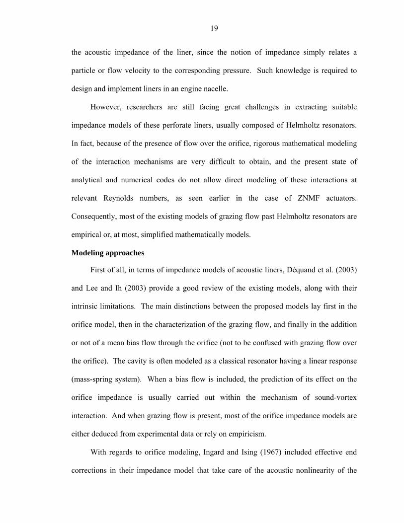
19

the acoustic impedance of the liner, since the notion of impedance simply relates a

particle or flow velocity to the corresponding pressure. Such knowledge is required to

design and implement liners in an engine nacelle.

However, researchers are still facing great challenges in extracting suitable

impedance models of these perforate liners, usually composed of Helmholtz resonators.

In fact, because of the presence of flow over the orifice, rigorous mathematical modeling

of the interaction mechanisms are very difficult to obtain, and the present state of

analytical and numerical codes do not allow direct modeling of these interactions at

relevant Reynolds numbers, as seen earlier in the case of ZNMF actuators.

Consequently, most of the existing models of grazing flow past Helmholtz resonators are

empirical or, at most, simplified mathematically models.

Modeling approaches

First of all, in terms of impedance models of acoustic liners, Déquand et al. (2003)

and Lee and Ih (2003) provide a good review of the existing models, along with their

intrinsic limitations. The main distinctions between the proposed models lay first in the

orifice model, then in the characterization of the grazing flow, and finally in the addition

or not of a mean bias flow through the orifice (not to be confused with grazing flow over

the orifice). The cavity is often modeled as a classical resonator having a linear response

(mass-spring system). When a bias flow is included, the prediction of its effect on the

orifice impedance is usually carried out within the mechanism of sound-vortex

interaction. And when grazing flow is present, most of the orifice impedance models are

either deduced from experimental data or rely on empiricism.

With regards to orifice modeling, Ingard and Ising (1967) included effective end

corrections in their impedance model that take care of the acoustic nonlinearity of the

20

orifice (mainly dependent on the ratio of the acoustic orifice momentum to the boundary

layer momentum when a grazing flow is included). Depending on the flow conditions of

the application, either low frequency or high frequency assumptions are used to model

the flow through the orifice. Also, standard assumption is that the orifice dimensions are

much smaller than the acoustic wavelength of interest.

Another important point to note is on the porosity factor of a perforate plate.

Because of the direct application of such a device to engine nacelle liners, the solution for

a single orifice impedance is usually derived and is then extended to multiple holes

geometry. The simple relation between the specific impedance of a perforate and a single

orifice, 0, 0pZ Z σ= , holds when the orifices are not too close from each other in order to

alleviate any jetting interaction effect between them. Here, the porosity factor is defined

by ( )holes hole area total areaNσ = × , where holesN is the number of orifices in the

perforate. Ingard (1953) states that the resonators can be treated independently of each

others if the distance between the orifices is greater than half of the acoustic wavelength.

Otherwise, to account for the interaction effect between multiple holes, Fok’s function is

usually employed (Melling 1973).

The grazing flow is commonly characterized as a fully-developed turbulent

boundary layer (or fully-developed turbulent pipe flow), although some investigations do

not, which may lead to difficulties for comparison sake. The parameters extracted from

the external boundary layer are usually the Mach number M∞ , friction velocity u∗ , or

boundary layer thickness δ .

Although most of the models are empirical or semi-empirical, some are still

analytical. The first models proposed were based on linear stability analysis where the

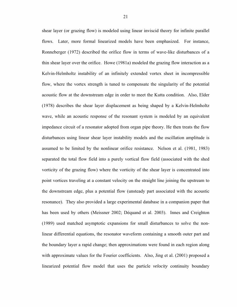
21

shear layer (or grazing flow) is modeled using linear inviscid theory for infinite parallel

flows. Later, more formal linearized models have been emphasized. For instance,

Ronneberger (1972) described the orifice flow in terms of wave-like disturbances of a

thin shear layer over the orifice. Howe (1981a) modeled the grazing flow interaction as a

Kelvin-Helmholtz instability of an infinitely extended vortex sheet in incompressible

flow, where the vortex strength is tuned to compensate the singularity of the potential

acoustic flow at the downstream edge in order to meet the Kutta condition. Also, Elder

(1978) describes the shear layer displacement as being shaped by a Kelvin-Helmholtz

wave, while an acoustic response of the resonant system is modeled by an equivalent

impedance circuit of a resonator adopted from organ pipe theory. He then treats the flow

disturbances using linear shear layer instability models and the oscillation amplitude is

assumed to be limited by the nonlinear orifice resistance. Nelson et al. (1981, 1983)

separated the total flow field into a purely vortical flow field (associated with the shed

vorticity of the grazing flow) where the vorticity of the shear layer is concentrated into

point vortices traveling at a constant velocity on the straight line joining the upstream to

the downstream edge, plus a potential flow (unsteady part associated with the acoustic

resonance). They also provided a large experimental database in a companion paper that

has been used by others (Meissner 2002; Déquand et al. 2003). Innes and Creighton

(1989) used matched asymptotic expansions for small disturbances to solve the non-

linear differential equations, the resonator waveform containing a smooth outer part and

the boundary layer a rapid change; then approximations were found in each region along

with approximate values for the Fourier coefficients. Also, Jing et al. (2001) proposed a

linearized potential flow model that uses the particle velocity continuity boundary

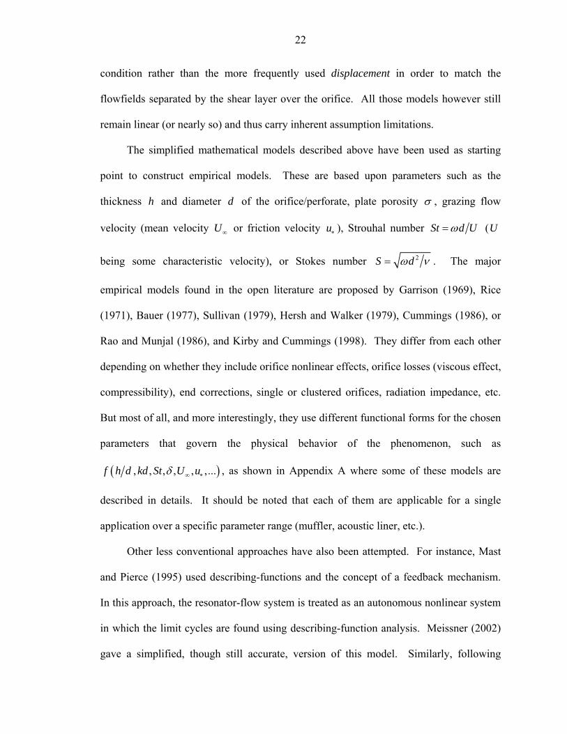
22

condition rather than the more frequently used displacement in order to match the

flowfields separated by the shear layer over the orifice. All those models however still

remain linear (or nearly so) and thus carry inherent assumption limitations.

The simplified mathematical models described above have been used as starting

point to construct empirical models. These are based upon parameters such as the

thickness h and diameter d of the orifice/perforate, plate porosity σ , grazing flow

velocity (mean velocity U∞ or friction velocity u∗ ), Strouhal number St d Uω= (U

being some characteristic velocity), or Stokes number 2S dω ν= . The major

empirical models found in the open literature are proposed by Garrison (1969), Rice

(1971), Bauer (1977), Sullivan (1979), Hersh and Walker (1979), Cummings (1986), or

Rao and Munjal (1986), and Kirby and Cummings (1998). They differ from each other

depending on whether they include orifice nonlinear effects, orifice losses (viscous effect,

compressibility), end corrections, single or clustered orifices, radiation impedance, etc.

But most of all, and more interestingly, they use different functional forms for the chosen

parameters that govern the physical behavior of the phenomenon, such as

( ), , , , , ,...f h d kd St U uδ ∞ ∗ , as shown in Appendix A where some of these models are

described in details. It should be noted that each of them are applicable for a single

application over a specific parameter range (muffler, acoustic liner, etc.).

Other less conventional approaches have also been attempted. For instance, Mast

and Pierce (1995) used describing-functions and the concept of a feedback mechanism.

In this approach, the resonator-flow system is treated as an autonomous nonlinear system

in which the limit cycles are found using describing-function analysis. Meissner (2002)

gave a simplified, though still accurate, version of this model. Similarly, following

23

Zwikker and Kosten’s (1949) theory for propagation of sound in channels, Sullivan

(1979) and Parrott and Jones (1995) used transmission matrices to model parallel-element

liner impedances. In another effort, Lee and Ih (2003) obtained an empirical model via

nonlinear regression analysis of results coming from various parametric tests.

Furthermore, acoustic eduction techniques have been used to determine the acoustic

impedance of liners, such as a finite element method (employed by NASA, see Watson et

al. 1998), that iterates on the numerical solution of the two dimensional convective wave

equation to determine an impedance that reproduces the measured amplitudes and phases

of the complex acoustic pressures; or a grazing flow data analysis program (employed by

Boeing, see Jones et al. (2003) and references therein for details) that conducts separate

computations in different regions to match the acoustic pressure and particle velocity

across the interfaces that determines the modal amplitudes in each of the regions; or also

a two dimensional modal propagation method based on insertion loss measurements

(employed by B. F. Goodrich, see Jones et al. (2003) and references therein for details)

that determines the frequency-dependent acoustic impedance of the test liner. Jones et al.

(2003) reviewed and compared these impedance eduction techniques.

Finally, as noted earlier, a few studies have been performed using numerical

simulations. Indeed, as can be seen in Liu and Long (1998) and Ozyörük and Long

(2000), it is computationally quite expensive, difficult to implement, and strong

limitations on the geometries are required. However, a promising numerical study by

Choudhari et al. (1999) gives valuable insight into the flow physics of these devices, such

as the effect of acoustic nonlinearity on the surface impedance.

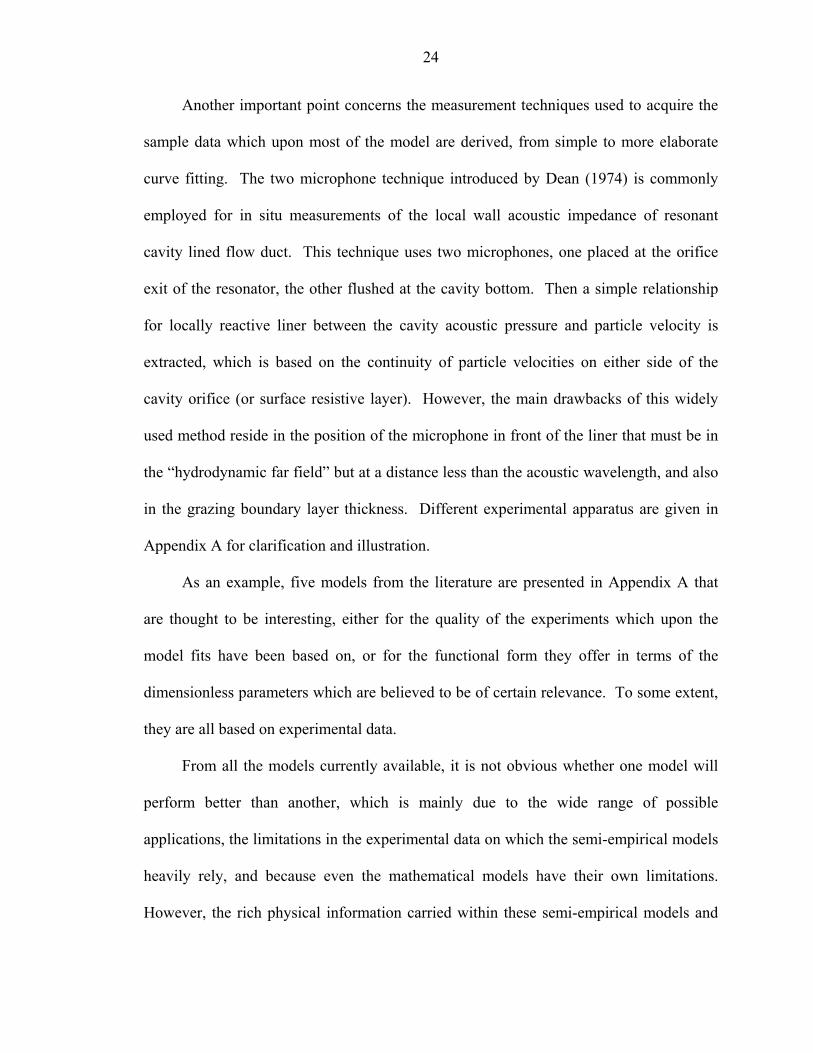
24

Another important point concerns the measurement techniques used to acquire the

sample data which upon most of the model are derived, from simple to more elaborate

curve fitting. The two microphone technique introduced by Dean (1974) is commonly

employed for in situ measurements of the local wall acoustic impedance of resonant

cavity lined flow duct. This technique uses two microphones, one placed at the orifice

exit of the resonator, the other flushed at the cavity bottom. Then a simple relationship

for locally reactive liner between the cavity acoustic pressure and particle velocity is

extracted, which is based on the continuity of particle velocities on either side of the

cavity orifice (or surface resistive layer). However, the main drawbacks of this widely

used method reside in the position of the microphone in front of the liner that must be in

the “hydrodynamic far field” but at a distance less than the acoustic wavelength, and also

in the grazing boundary layer thickness. Different experimental apparatus are given in

Appendix A for clarification and illustration.

As an example, five models from the literature are presented in Appendix A that

are thought to be interesting, either for the quality of the experiments which upon the

model fits have been based on, or for the functional form they offer in terms of the

dimensionless parameters which are believed to be of certain relevance. To some extent,

they are all based on experimental data.

From all the models currently available, it is not obvious whether one model will

perform better than another, which is mainly due to the wide range of possible

applications, the limitations in the experimental data on which the semi-empirical models

heavily rely, and because even the mathematical models have their own limitations.

However, the rich physical information carried within these semi-empirical models and

25

the corresponding data on which they are based will undoubtfully aid the development of

reduced-order models in ZNMF actuator interacting with a grazing flow.

Unresolved Technical Issues

By surveying the literature, i.e. looking at the flow mechanism of isolated ZNMF

actuators to more complex behavior when the actuator is interacting with an incoming

boundary layer, along with examples of sound absorber technology, several key issues

can be highlighted that still remain to be addressed. This subsection lists the principal

ones.

Fundamental flow physics. Clearly, there still exists a lack in the fundamental

understanding of the flow mechanisms that govern the dynamics of ZNMF actuators.

While the cavity design is well understood, the orifice modeling and especially the effect

of the interaction with an external boundary layer requires more in-depth consideration.

Also, whether performing experimental studies or numerical simulations, researchers are

confronted with a huge parameter space that is time consuming and requires expensive

experiments or simulations. Hence the development of simple physics-based reduced-

order models is primordial.

2D vs. 3D. While most of the numerical simulations are performed for two-

dimensional problems, three-dimensionality effects clearly can be important, especially

to model the flow coming out of a circular orifice as shown in Rizzeta et al. (1998) or

Ravi et al. (2004) that also found distinct and non negligible three-dimensional effects of

the flow.

Compressibility effects. Usually, the entire flow field is numerically solved using

an incompressible solver. However, such an assumption, although valid outside the

actuator, may be violated inside the orifice at high jet velocity and, more generally, inside

26

the cavity due to the acoustic compliance of the cavity. Indeed, the cavity acts like a

spring that stores the potential energy produced by the driver motion.

Lack of high-resolution experimental data. Most of the experimental studies

employed either Hot Wire Anemometry (HWA), Particle Image Velocimetry (PIV) or

Laser Doppler Velocimetry (LDV) to measure the flow. However, each of these

techniques has shortcomings, as briefly enumerated below.

In the case of HWA, since the flow is highly unsteady and by definition oscillatory,

its deployment must be carefully envisaged, especially considering the de-rectification

procedure used to obtain the reversal flow. Since it is an intrusive technique that may

perturb the flow, other issues are that it is a single point measurement (hence the need to

traverse the whole flow field), problems arise with measurements near zero velocity

(transition from free to forced convection), and the accuracy may be affected by the

calibration (sensitivity), the local temperature, or some conductive heat loss.

With regards to PIV, although the main advantage resides in the fact that it is a

non-intrusive flow visualization technique that captures instantaneous snapshots of the

flow field, the micro/meso scale of ZNMF devices requires very high resolution in the

vicinity of the actuator orifice in order to obtain reasonable accuracy in the data. This is

difficult to achieve using a standard digital PIV system.

Finally, a large number of samples are required in order to get proper accuracy in

the data from LDV measurement, and excellent spatial resolution is difficult to achieve

due to the finite length of the probe volume. Also, since LDV is a single point

measurement, a traversing probe is required in order to map the entire flow field.

27

Lack of accurate low-order models. Clearly, the few reduced-order models that

are present so far are not sufficient to be able to capture the essential dynamics of the

flow generated by a ZNMF actuator. Better models must be constructed to account for

the slot geometry and the impact of the crossflow on the jet velocity profile. The five

models of grazing flow past Helmholtz resonators summarized in Appendix A reveal the

disparity in the impedance expressions as well as in the range of applications (see Table

A-1). Clearly, the task of extracting a validated semi-empirical model is far from trivial.

But leveraging past experience is critical to yielding accurate low-order models for

implementation of a ZNMF actuator.

Objectives

The literature survey presented above has permitted the identification of key

technical issues that remain to be resolved in order to fully implement ZNMF actuators

into realistic applications. Currently, it is difficult for a prospective user to successfully

choose and use the appropriate actuator that will satisfy specific requirements. Even

though many designs have been used in the literature, no studies have systematically

studied the optimal design of these devices. For instance, how large should the cavity

be? What type of driver is most appropriate to a specific application? Possibilities

include a low cost, low power piezoelectric-diaphragm, an electromagnetic or mechanical

piston that will provide large flow rate but may require significant power, or a voice-coil

speaker typically used in audio applications? What orifice geometry should be chosen?

Options include sharp versus rounded edges, large versus short thickness, an

axisymmetric versus a rectangular slot? Clearly, no validated tools are currently

available for end users to address these questions. Generally, a trial and error method

28

using expensive experimental studies and/or time consuming numerical simulations have

been employed.

The present work seeks to address these issues by providing a clear physical

understanding of how these devices behave and interact with and without an external

flow, and by developing and validating reduced-order dynamical models and scaling

laws. Successful completion of these objectives will ultimately aid in the analysis and

development of design tools for sizing, design and deployment of ZNMF actuators in

flow control applications.

Approach and Outline of Thesis

To reach the stated objectives, the following technical approach has been

employed. First, the identification of outstanding key issues and the formulation of the

problem have been addressed in this chapter by surveying the literature concerning the

modeling in diverse applications of ZNMF actuators and acoustic liner technology. The

relevant information about the key device parameters and flow conditions (like the driver

configuration, cavity, orifice shape, or the external boundary layer parameters) are thus

extracted. Before investigating how a ZNMF device interacts with an external boundary

layer, the case of an isolated ZNMF actuator must be fully understood and documented.

This is the subject of Chapter 2. An isolated ZNMF device is first characterized and the

relevant parameters are defined. Then, the previous work done by the author in Gallas et

al. (2003a) is summarized. Their work discusses a lumped element model of a

piezoelectric-driven ZNMF actuator. One goal of the present work is to extend their

model to more general devices and to remove, as far as possible, some restricting

limitations, especially on the orifice loss coefficient. Consequently, a thorough

nondimensional analysis is first carried out to extract the physics behind such a device.

29

Also, some relevant modeling issues are discussed and reviewed, for instance on

the orifice geometry effects and the driving transducer dynamics. Then, to study in great

details the dynamics of isolated ZNMF actuators, an extensive experimental investigation

is proposed where various test actuator configurations are examined over a wide range of

operating conditions. The experimental setup is described in Chapter 3.

30

CHAPTER 2

DYNAMICS OF ISOLATED ZERO-NET MASS FLUX ACTUATORS

Several key issues were highlighted in the introduction chapter that will be

addressed in this thesis. This Chapter is first devoted to familiarize the reader with the

dynamics of ZNMF actuators, their behavior and inherent challenges in developing tools

to accurately model them. One goal, before addressing the general case of the interaction

with an external boundary layer, is to understand the nonlinear dynamics of an isolated

ZNMF actuator. This chapter is therefore entirely dedicated to the analysis of isolated

ZNMF actuators issuing into a quiescent medium, as outlined below.

The device is first characterized and the relevant parameters defined in order to

clearly define the scope of the present investigation. The previous work performed by

the author in Gallas et al. (2003a) is next summarized. Their work discusses a lumped

element model of a piezoelectric-driven ZNMF actuator that relates the output volume

flow rate to the input voltage in terms of a transfer function. Their model is extended to

more general devices and solutions to remove some restricting limitations are explored.

Based on this knowledge, a thorough dimensional analysis is then carried out to extract

the physics behind an isolated ZNMF actuator. A dimensionless linear transfer function

is also derived for a generic driver configuration, which is thought to be relevant as a

design tool. It is shown that a compact expression can be obtained regardless of the

orifice geometry and regardless of the driver configuration. Finally, relevant modeling

issues pointed out in the first chapter are discussed and reviewed. Some issues are then

addressed, more particularly on the modeling of the orifice flow where a temporal

31

analysis of the existing lumped element model is proposed along with a physically-based

discussion on the orifice loss mechanism. Issues on the dynamics of the driving

transducer are discussed as well. Finally, a test matrix constructed to study the ZNMF

actuator dynamics is presented.

Characterization and Parameter Definitions

Figure 1-1 shows a typical ZNMF actuator, where the geometric parameters are

shown. First of all, it is worthwhile to define some precise quantities of interest that have

been used in the published literature and try to unify them into a generalized form. For

instance, people have used the impulse stroke length, some spatially or time averaged exit

velocities, or Reynolds numbers based either on the circulation of vortex rings or on an

averaged jet velocity to characterize the oscillating orifice jet flow. Here, an attempt to

unify them is made.

The inherent nature of the jet is both a function of time (oscillatory motion) and of

space (velocity distribution across the orifice exit area). It is also valuable to distinguish

the ejection from the ingestion portion of a cycle. Many researchers (Smith and Glezer

1998, Glezer and Amitay 2002) characterize a synthetic jet based on a simple “slug

velocity profile” model that includes a dimensionless stroke length 0L d and a Reynolds

number ReCLV CLV d ν= based on the velocity scale (average orifice velocity) such that

( )/ 2

0 0

T

CL CLV fL f v t dt= = ∫ , (2-1)

where ( )CLv t is the centerline velocity, 1T f= is the period, thereby 2T representing

half the period or the time of discharge for a sinusoidal signal, and 0L is the distance that

32

a “slug” of fluid travels away from the orifice during the ejection portion of the cycle or

period.

In addition, Smith and Glezer (1998) have employed a Reynolds number based on

the impulse per unit length (i.e., the momentum associated with the ejection per unit

width), 0 0ReI I dµ= , where the impulse per unit width is defined as

( )2 2

0 0

T

CLI d v t dtρ= ∫ . (2-2)

Or similarly, following the physics of vortex ring formation (Glezer 1988), a

Reynolds number, 0Re νΓ = Γ , is used based on the initial circulation associated with the

vortex generation process, with 0Γ defined by

( )2 2 2

0 0

1 12 2 2

T

CL CLTv t dt VΓ = =∫ . (2-3)

Alternatively (Utturkar et al. 2003), a spatial and time-averaged exit velocity during

the expulsion stroke is used to define the Reynolds number Re jV d ν= , where the time-

averaged exit velocity jV is defined as

( ) ( )2 2

0 0

2 1 2 ˆ,n

T T

j nSn

V v t x dtdS v t dtT S T

= =∫ ∫ ∫ , (2-4)

where ( )v t is the spatial averaged velocity, nS is the exit area of the orifice neck, and x

is the cross-stream coordinate (see Figure 1-2 for coordinates definition). For general

purposes, instead of limiting ourselves to a simple uniform “slug” profile, the latter

definition is considered throughout this dissertation.

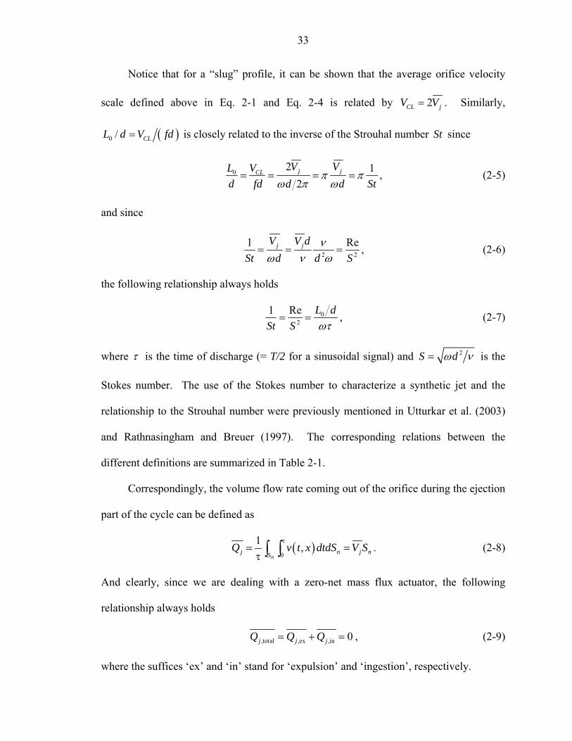
33

Notice that for a “slug” profile, it can be shown that the average orifice velocity

scale defined above in Eq. 2-1 and Eq. 2-4 is related by 2CL jV V= . Similarly,

( )0 / CLL d V fd= is closely related to the inverse of the Strouhal number St since

0 2 12j jCL V VL V

d fd d d Stπ π

ω π ω= = = = , (2-5)

and since

2 2

1 Rej jV V dSt d d S

νω ν ω

= = = , (2-6)

the following relationship always holds

02

1 Re L dSt S ωτ

= = , (2-7)

where τ is the time of discharge (= T/2 for a sinusoidal signal) and 2S d= ω ν is the

Stokes number. The use of the Stokes number to characterize a synthetic jet and the

relationship to the Strouhal number were previously mentioned in Utturkar et al. (2003)

and Rathnasingham and Breuer (1997). The corresponding relations between the

different definitions are summarized in Table 2-1.

Correspondingly, the volume flow rate coming out of the orifice during the ejection

part of the cycle can be defined as

( )0

1 ,n

j n j nSQ v t x dtdS V S

τ= =τ ∫ ∫ . (2-8)

And clearly, since we are dealing with a zero-net mass flux actuator, the following

relationship always holds

,total ,ex ,in 0j j jQ Q Q= + = , (2-9)

where the suffices ‘ex’ and ‘in’ stand for ‘expulsion’ and ‘ingestion’, respectively.

34

Table 2-1: Correspondence between synthetic jet parameter definitions

0Ld

1ωτ

⎛ ⎞→ × →⎜ ⎟⎝ ⎠

2

1 ReSt S

=

0ReI ,

0ReΓ → Re

As seen from the above definitions, once a velocity or time scale has been chosen, a

length scale must be similarly selected for the orifice or slot. Figure 1-3 show two typical

orifice geometries encountered in a ZNMF actuator, and give the geometric parameters

and coordinates definition. Notice that the orifice is straight in both cases. No beveled,

rounded or other shapes are taken into account, although other geometries have been

investigated (Bridges and Smith 2001; Smith and Swift 2003b; Milanovic & Zaman

2005; Shuster and Smith 2004). Throughout this dissertation, the primary length scale

used is the diameter or depth of the orifice d . The spanwise orifice width w is used as

needed for discussions related to a rectangular slot, and the height h is a third

characteristic dimension. Clearly, if d is chosen as the characteristic length scale, then

w d and h d are key nondimensional parameters.

Lumped Element Modeling

Summary of Previous Work

A lumped element model of a piezoelectric-driven synthetic jet actuator exhausting

in a quiescent medium has been recently developed and compared with experiments by

Gallas et al. (2003a). In lumped element modeling (LEM), the individual components of

a synthetic jet are modeled as elements of an equivalent electrical circuit using conjugate

power variables (i.e., power = generalized flow x generalized effort). The frequency

response function of the circuit is derived to obtain an expression for j acQ V , the volume

flow rate per applied voltage. LEM provides a compact analytical model and valuable

35

physical insight into the dependence of the device behavior on geometric and material

properties. Methods to estimate the parameters of the lumped element model were

presented and experiments were performed to isolate different components of the model

and evaluate their suitability. The model was applied to two prototypical synthetic jets

and found to provide very good agreement with the measured performance. The results

reveal the advantages and shortcomings of the model in its present form. With slight

modifications, the model is applicable to any type of ZNMF device.

PiezoceramicComposite Diaphragm

Orifice

Cavity

Vac

1:φa

P

I

MaD

Qd

RaN MaN

MaRad

RaOQc

Qj

Ceb

CaD

CaC

i

I-i

Vac

electricaldomain

acoustic/fluidicdomain

RaD

electroacousticcoupling

d

h( )∀

Figure 2-1: Equivalent circuit model of a piezoelectric-driven synthetic jet actuator.

The equivalent circuit model is shown in Figure 2-1. The structure of the

equivalent circuit is explained as follows. An ac voltage acV is applied across the

piezoceramic to create an effective acoustic pressure that drives the diaphragm into

oscillatory motion. This represents a conversion from the electrical to the acoustic

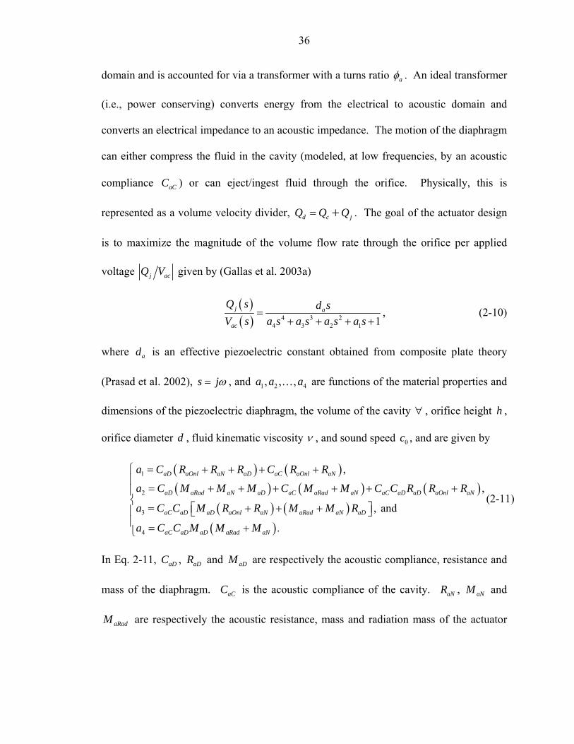
36

domain and is accounted for via a transformer with a turns ratio aφ . An ideal transformer

(i.e., power conserving) converts energy from the electrical to acoustic domain and

converts an electrical impedance to an acoustic impedance. The motion of the diaphragm

can either compress the fluid in the cavity (modeled, at low frequencies, by an acoustic

compliance aCC ) or can eject/ingest fluid through the orifice. Physically, this is

represented as a volume velocity divider, d c jQ Q Q= + . The goal of the actuator design

is to maximize the magnitude of the volume flow rate through the orifice per applied

voltage j acQ V given by (Gallas et al. 2003a)

( )( ) 4 3 2

4 3 2 1 1j a

ac

Q s d sV s a s a s a s a s

=+ + + +

, (2-10)

where ad is an effective piezoelectric constant obtained from composite plate theory

(Prasad et al. 2002), s jω= , and 1 2 4, , ,a a a… are functions of the material properties and

dimensions of the piezoelectric diaphragm, the volume of the cavity ∀ , orifice height h ,

orifice diameter d , fluid kinematic viscosity ν , and sound speed 0c , and are given by

( ) ( )( ) ( ) ( )

( ) ( )( )

1

2

3

4

,

,

, and

.

aD aOnl aN aD aC aOnl aN

aD aRad aN aD aC aRad aN aC aD aD aOnl aN

aC aD aD aOnl aN aRad aN aD

aC aD aD aRad aN

a C R R R C R R

a C M M M C M M C C R R R

a C C M R R M M R

a C C M M M

= + + + +⎧⎪

= + + + + + +⎪⎨

= + + +⎡ ⎤⎪ ⎣ ⎦⎪ = +⎩

(2-11)

In Eq. 2-11, aDC , aDR and aDM are respectively the acoustic compliance, resistance and

mass of the diaphragm. aCC is the acoustic compliance of the cavity. aNR , aNM and

aRadM are respectively the acoustic resistance, mass and radiation mass of the actuator

37

orifice, while aOnlR represents the nonlinear resistance term associated with the orifice

flow discharge and is a function of the volume flow rate jQ .

0 500 1000 1500 2000 2500 30000

5

10

15

20

25

30

35

Frequency (Hz)

Mag

nitu

de o

f max

imum

vel

ocity

(m/s

)

0 500 1000 15000

10

20

30

40

50

60

70

Frequency (Hz)

Mag

nitu

de o

f max

imum

vel

ocity

(m/s

) Figure 2-2: Comparison between the lumped element model and experimental frequency

response measured using phase-locked LDV for two prototypical synthetic jets (Gallas et al. 2003a).

The lumped parameters in the circuit in Figure 2-1 represent generalized energy

storage elements (i.e., capacitors and inductors) and dissipative elements (i.e., resistors).

Model parameter estimation techniques, assumptions, and limitations are discussed in

Gallas et al. (2003a). The capability of the technique to describe the measured frequency

response of two prototypical synthetic jets is shown in Figure 2-2. The case in the left

half of the figure reveals the 4th-order nature of the frequency response. The two

resonance peaks are related to the diaphragm natural frequency df and the Helmholtz

frequency Hf , thereby demonstrating the potential significance of compressibility

effects. The case in the right half of the figure reveals how the model can be “tuned” to

produce a device with a single resonance frequency with large output velocities.

The important point is that the model gives a reasonable estimate of the output of

interest (typically within ±20%) with minimal effort. The power of LEM is its simplicity

38

and its usefulness as a design tool. LEM can be used to provide a reasonable estimate of

the frequency response of the device as a function of the signal input, device geometry,

and material and fluid properties.

Limitations and Extensions of Existing Model

The study performed in Gallas et al. (2003a) was restricted to axisymmetric orifice

geometry and the oscillating pressure driven flow inside the pipe was assumed to be

laminar and fully-developed. Also, a piezoelectric-diaphragm was chosen to drive the

actuator.

A straightforward extension of their model is that of a rectangular slot model.

Appendix C provides a derivation of the solution of oscillating pressure driven flow in a

2D channel, assuming the flow is laminar, incompressible and fully-developed. The low

frequency approximation then yields the lumped element parameters. Hence, for a 2D

channel orifice the acoustic resistance and mass are found to be, respectively,

( )33

2 2aN

hRw dµ

= , and ( )

35 2aN

hMw dρ

= . (2-12)

Similarly, also of interest is the acoustic radiation impedance for a rectangular slot. The

acoustic radiation mass aRadM is modeled for 1kd < as a rectangular piston in an infinite

baffle by assuming that the rectangular slot is mounted in a plate that is much larger in

extent than the slot size (Meissner 1987),

( ) ( )

02 2

1ln 2 2 1 6aRad aRad

c w dX M kdwd d w k wρω

π π

⎡ ⎤⎢ ⎥= = +

−⎢ ⎥⎣ ⎦, (2-13)

where aRadX corresponds to the acoustic radiation reactance.

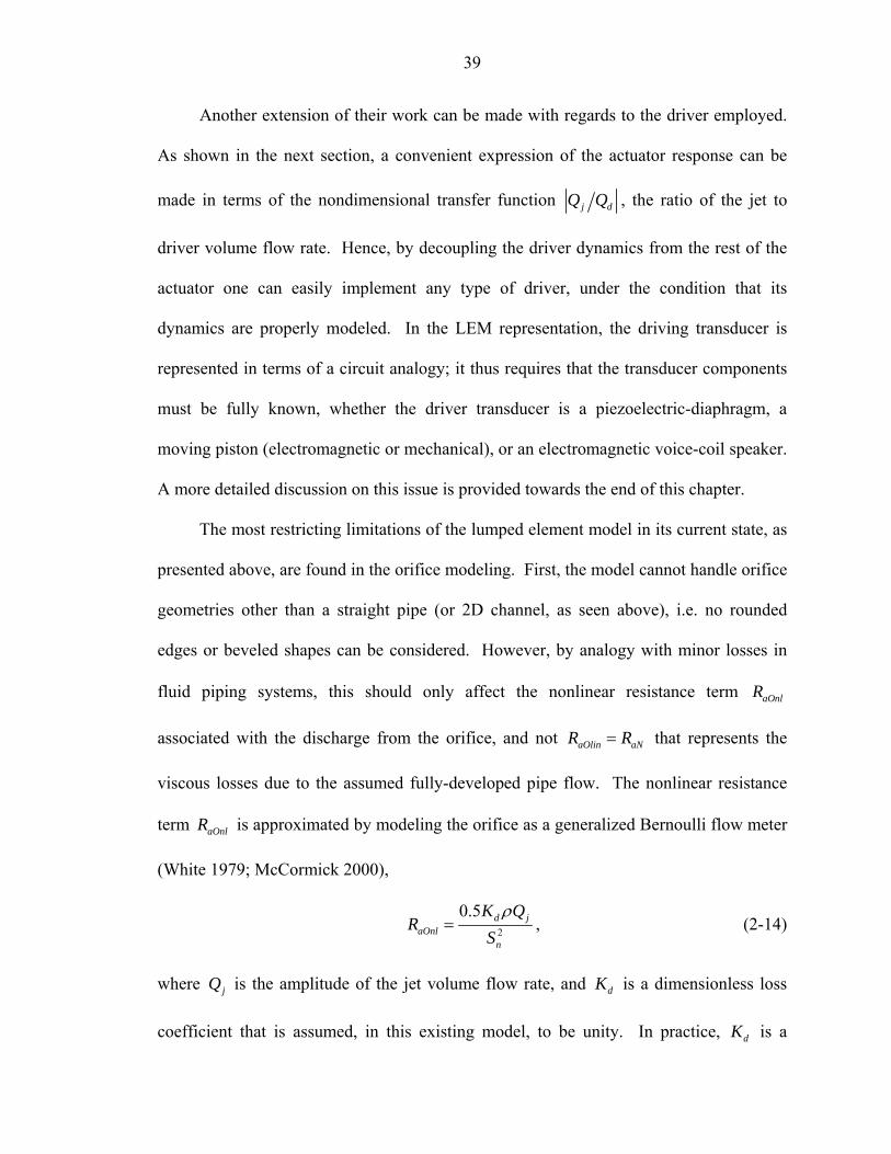
39

Another extension of their work can be made with regards to the driver employed.

As shown in the next section, a convenient expression of the actuator response can be

made in terms of the nondimensional transfer function j dQ Q , the ratio of the jet to

driver volume flow rate. Hence, by decoupling the driver dynamics from the rest of the

actuator one can easily implement any type of driver, under the condition that its

dynamics are properly modeled. In the LEM representation, the driving transducer is

represented in terms of a circuit analogy; it thus requires that the transducer components

must be fully known, whether the driver transducer is a piezoelectric-diaphragm, a

moving piston (electromagnetic or mechanical), or an electromagnetic voice-coil speaker.

A more detailed discussion on this issue is provided towards the end of this chapter.

The most restricting limitations of the lumped element model in its current state, as

presented above, are found in the orifice modeling. First, the model cannot handle orifice

geometries other than a straight pipe (or 2D channel, as seen above), i.e. no rounded

edges or beveled shapes can be considered. However, by analogy with minor losses in

fluid piping systems, this should only affect the nonlinear resistance term aOnlR

associated with the discharge from the orifice, and not aOlin aNR R= that represents the

viscous losses due to the assumed fully-developed pipe flow. The nonlinear resistance

term aOnlR is approximated by modeling the orifice as a generalized Bernoulli flow meter

(White 1979; McCormick 2000),

2

0.5 d jaOnl

n

K QR

Sρ

= , (2-14)

where jQ is the amplitude of the jet volume flow rate, and dK is a dimensionless loss

coefficient that is assumed, in this existing model, to be unity. In practice, dK is a

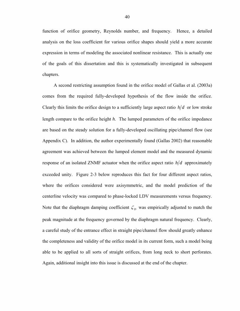
40

function of orifice geometry, Reynolds number, and frequency. Hence, a detailed

analysis on the loss coefficient for various orifice shapes should yield a more accurate

expression in terms of modeling the associated nonlinear resistance. This is actually one

of the goals of this dissertation and this is systematically investigated in subsequent

chapters.

A second restricting assumption found in the orifice model of Gallas et al. (2003a)

comes from the required fully-developed hypothesis of the flow inside the orifice.

Clearly this limits the orifice design to a sufficiently large aspect ratio h d or low stroke

length compare to the orifice height h. The lumped parameters of the orifice impedance

are based on the steady solution for a fully-developed oscillating pipe/channel flow (see

Appendix C). In addition, the author experimentally found (Gallas 2002) that reasonable

agreement was achieved between the lumped element model and the measured dynamic

response of an isolated ZNMF actuator when the orifice aspect ratio h d approximately

exceeded unity. Figure 2-3 below reproduces this fact for four different aspect ratios,

where the orifices considered were axisymmetric, and the model prediction of the

centerline velocity was compared to phase-locked LDV measurements versus frequency.

Note that the diaphragm damping coefficient Dζ was empirically adjusted to match the

peak magnitude at the frequency governed by the diaphragm natural frequency. Clearly,

a careful study of the entrance effect in straight pipe/channel flow should greatly enhance

the completeness and validity of the orifice model in its current form, such a model being

able to be applied to all sorts of straight orifices, from long neck to short perforates.

Again, additional insight into this issue is discussed at the end of the chapter.

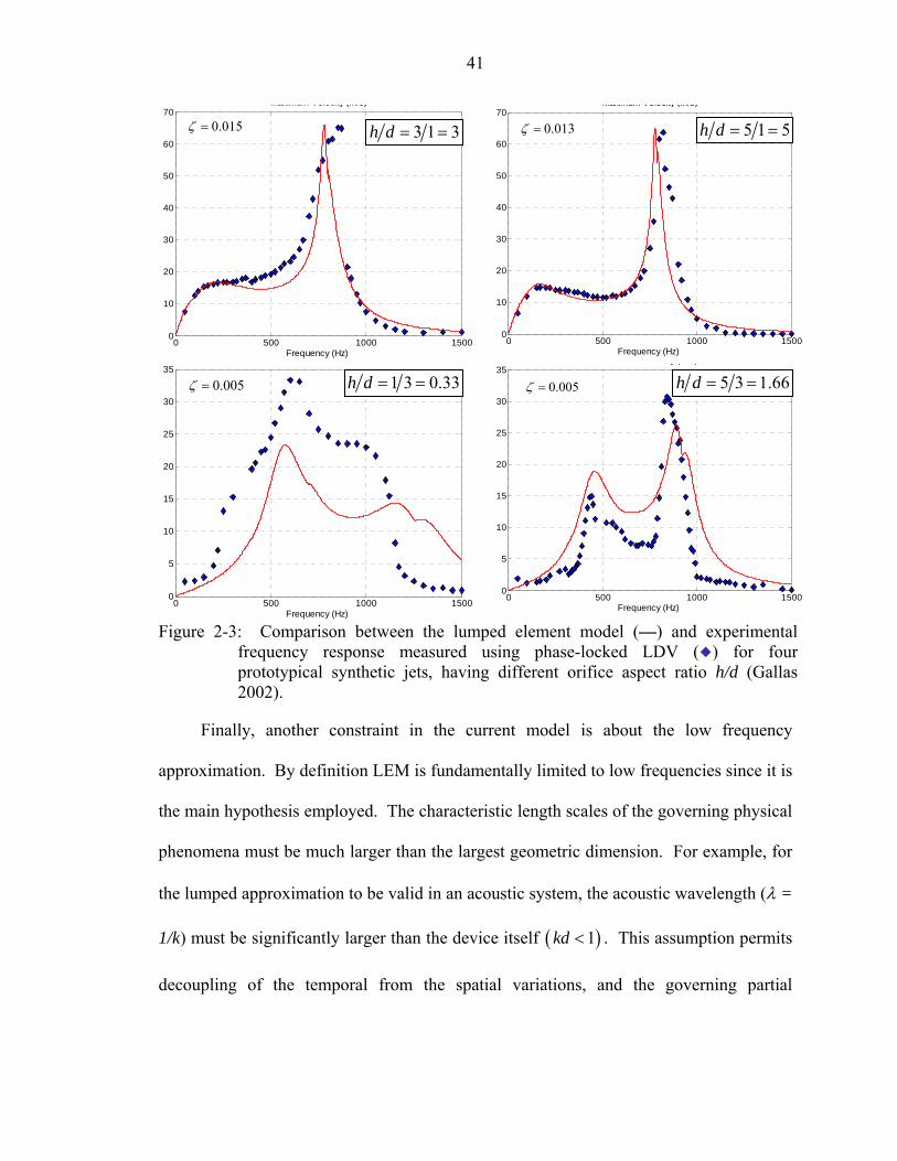
41

0 500 1000 15000

10

20

30

40

50

60

70

Frequency (Hz)

Maximum Velocity (m/s)

0.015ζ =

0 500 1000 15000

10

20

30

40

50

60

70

Frequency (Hz)


0.015ζ =

0 500 1000 15000

10

20

30

40

50

60

70

Frequency (Hz)


0.013ζ =

0 500 1000 15000

10

20

30

40

50

60

70

Frequency (Hz)


0.013ζ =

0 500 1000 15000

5

10

15

20

25

30

35

Frequency (Hz)

y ( )

0.005ζ =

0 500 1000 15000

5

10

15

20

25

30

35

Frequency (Hz)

y ( )

0.005ζ =

0 500 1000 15000

5

10

15

20

25

30

35

Frequency (Hz)

y ( )

0.005ζ =

0 500 1000 15000

5

10

15

20

25

30

35

Frequency (Hz)

y ( )

0.005ζ =

Figure 2-3: Comparison between the lumped element model (—) and experimental frequency response measured using phase-locked LDV ( ) for four prototypical synthetic jets, having different orifice aspect ratio h/d (Gallas 2002).

Finally, another constraint in the current model is about the low frequency

approximation. By definition LEM is fundamentally limited to low frequencies since it is

the main hypothesis employed. The characteristic length scales of the governing physical

phenomena must be much larger than the largest geometric dimension. For example, for

the lumped approximation to be valid in an acoustic system, the acoustic wavelength (λ =

1/k) must be significantly larger than the device itself ( )1kd < . This assumption permits

decoupling of the temporal from the spatial variations, and the governing partial

3 1 3h d = = 5 1 5h d = =

1 3 0.33h d = = 5 3 1.66h d = =

42

differential equations for the distributed system can be “lumped” into a set of coupled

ordinary differential equations.

0 0.2 0.4 0.6 0.8 10

0.1

0.2

0.3

0.4

0.5

0.6

0.7

0.8

0.9

1

x/(d/2)

v/v m

ax

S=1S=12S=20S=50

Figure 2-4: Variation in velocity profile vs. S = 1, 12, 20, and 50 for oscillatory pipe

flow in a circular duct.

However, it is well known that the flow inside a long pipe/channel is frequency

dependent, as shown in Figure 2-4 and Figure 2-5. From Figure 2-4, it can be seen that,

as the Stokes number S goes to zero, the velocity profile asymptotes to Poiseuille flow,

while as S increases, the thickness of the Stokes layer decreases below 2d , leading to

an inviscid core surrounded by a viscous annular region where a phase lag is also present

between the pressure drop across the orifice and the velocity profile. Figure 2-5 shows

that the ratio of the spatial average velocity ( )ˆ jv t to the centerline velocity ( )CLv t , which

is 0.5 for Poiseuille flow, is strongly dependant on the Stokes number. Although it has

been shown (Gallas et al. 2003a) that the acoustic reactance is approximately constant

with frequency, the acoustic resistance, which does asymptote at low frequencies to the

steady value given by the lumped element model, gradually increases with frequency.

43

Therefore, this frequency-dependence estimate should not be disregarded, and care must

be taken in the frequency range at which ZNMF actuators are running to apply LEM. For

instance, the frequency dependence given by Figure 2-5 can be easily implemented in the

present model to provide estimates for the acoustic impedance of the orifice, as discussed

in Gallas et al. (2003a).

1 10 1000.5

0.55

0.6

0.65

0.7

0.75

0.8

0.85

0.9

0.95

1

S=(ωd2/ν)1/2

v / v

CL

⟨

Figure 2-5: Ratio of spatial average velocity to centerline velocity vs. Stokes number for

oscillatory pipe flow in a circular duct.

To summarize this section, the model given in Gallas et al. (2003a) has been

presented and reviewed, and it has been shown that it could be extended to more general

device configurations, particularly in terms of orifice geometry and driver configuration.

Also, some of their restricting assumption limits could be, if not completely removed, at

least greatly attenuated, and this is further analyzed and discussed in the last part of this

chapter. But before, a general dimensional analysis of an isolated actuator is carried out

in the next section that gives valuable insight on the parameter space and on the system

response behavior.

44

Dimensional Analysis

Definition and Discussion

In the first section of this chapter, the primary output variables of interest have been

defined, and specifically the spatial and time-averaged ejection velocity of the jet jV

defined in Eq. 2-4. It is then interesting to rewrite them in terms of pertinent

dimensionless parameters. Using the Buckingham-Pi theorem (Buckingham 1914), the

dependence of the jet output velocity can be written in terms of nondimensional

parameters. The derivation is presented in full in Appendix D and the results are

summarized below:

3, , , , , ,Re

j d

H d

Q Qh wSt fn kd Sd d d

ω ωω ω

⎫⎪ ⎛ ⎞∆∀⎪ =⎬ ⎜ ⎟

⎝ ⎠⎪⎪⎭

. (2-15)

The quantities in the left hand side of the functional are possible choices that the

dependent variable jV can take. j dQ Q represents the ratio of the volume flow rate of

the driver ( )d dQ ω= ∆∀ to the jet volume flow rate of the ejection part. St is the

Strouhal number and Re is the jet Reynolds number defined earlier. Notice the close

relationship between the jet Reynolds number, the Stokes number and the Strouhal

number that were given by Eq. 2-7 and found again here by manipulation of the Π -

groups (see Appendix D for details). Therefore, for a given geometric configuration,

either the Strouhal or the Reynolds numbers along with the Stokes number could suffice

to characterize the jet exit behavior. It is also interesting to view Eq. 2-7 as the basis for

the jet formation criterion defined by Utturkar et al. (2003). Actually, it is intrusive to

look at the different physical interpretations that the Strouhal number can take. In the

45

fluid dynamics community, it is usually defined as the ratio of the unsteady to the steady

inertia. However, it can also be interpreted as the ratio of 2 length scales or 2 time scales,

such that

0

oscillation

convection

j j

j j

d d dStLV V

tdSttV V d

ωω

ω ω

⎧ = = ≈⎪⎪⎨⎪ = = ≈⎪⎩

(2-16)

where 0d L is the ratio of a typical length scale d of the orifice to the particle excursion

L0 through the orifice. The Strouhal number can also be the ratio of the oscillation time

scale to the convective time scale.

The physical significance of each term in the RHS of Eq. 2-15 is described below:

• Hω ω is the ratio of the driving frequency to the Helmholtz frequency

0H nc S h′= ∀ω (see Appendix B for a complete discussion on the definition and derivation of Hω ), a measure of the compressibility of the flow inside the cavity.

• h d is the orifice/slot height to diameter aspect ratio.

• w d is the orifice/slot width to diameter aspect ratio.

• dω ω is the ratio of the operating frequency to the natural frequency of the driver.

• 3d∆∀ is the ratio of the displaced volume by the driver to the orifice diameter cubed.

• kd d λ= is the ratio of the orifice diameter to the acoustic wavelength.

• 2S d= ω ν is the Stokes number, the ratio of the orifice diameter to the unsteady

boundary layer thickness in the orifice ν ω .

It is evident that in the case of an isolated ZNMF actuator, the response is strongly

dependant on the geometric parameters , , ,H h d w d kdω ω and the operating

46

conditions 3, ,d d Sω ω ∆∀ . In fact, from the functional form described by Eq. 2-15

and for a given device with fixed dimensions and a given fluid, the actuator output is only

dependent on the driver dynamics ( ),dω ∆∀ and the actuation frequency ω .

Although compressibility effects in the orifice are neglected in this dissertation, it

warrants a few lines. Compressibility will occur in the orifice for high Mach number

flows and/or for high density flows. If the compressibility of the fluid has to be taken

into account, it follows by definition that density must be considered as a new variable.

For instance, the pressure is now coupled to the temperature and density through the

equation of state. Similarly, the continuity equation is no longer trivial. Also,

temperature is important, and one has to reminder that the variation of the thermal

conductivity k and dynamic viscosity µ - that are transport quantities – with temperature

may be important.

Dimensionless Linear Transfer Function for a Generic Driver

Valuable physical insight into the dependence of the device behavior on geometry

and material properties is provided by the frequency response of the ZNMF actuator

device. In order to obtain an expression of the linear transfer function of the jet output to

the input signal to the actuator, the compact nonlinear analytical model given by LEM is

used in a similar manner as described and introduced in the previous section, since it was

shown to be a valuable design tool. Notice however that the nonlinear part of the model

in its present form -only confined in the orifice- is neglected for simplicity in this

analysis. Figure 2-6 shows a schematic representation of a ZNMF actuator having a

generic driver using LEM. This representation enables us to bypass the need of an

47

expression for the acoustic impedance aDZ of the driving transducer, although it lacks its

dynamics modeling.

QdZaD

ZaC ZaO

(Qd-Qj)

Qj

Figure 2-6: Schematic representation of a generic-driver ZNMF actuator.

In this case, a convenient representation of the transfer function is to normalize the

jet volume flow rate by the driver volume flow rate, j dQ Q , and obtain an expression via

the current/flow divider shown in Figure 2-6,

( )( )

2

11

1

1

j aC aC

d aC aO aC aO aO

aC aO

aO

aC aO aO

Q s Z sCQ s Z Z sC R sM

C MR s s

C M M

= =+ + +

=+ +

(2-17)

assuming that the acoustic orifice impedance aO aO aOZ R M= + only contains the linear

resistance aNR and the radiation mass aRadM is neglected or added to aOM .

Knowing that the Helmholtz resonator frequency of the actuator is defined by

1H

aC aOC Mω = , (2-18)

and the damping ratio of the system by

12

aCaN

aO

CRM

ζ = , (2-19)

by substituting in Eqs. 2-18 and 2-19, Eq. 2-17 can then be rewritten as

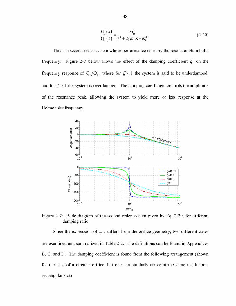
48

( )( )

2

2 22j H

d H H

Q sQ s s s

ωζω ω

=+ +

. (2-20)

This is a second-order system whose performance is set by the resonator Helmholtz

frequency. Figure 2-7 below shows the effect of the damping coefficient ζ on the

frequency response of j dQ Q , where for 1ζ < the system is said to be underdamped,

and for 1ζ > the system is overdamped. The damping coefficient controls the amplitude

of the resonance peak, allowing the system to yield more or less response at the

Helmoholtz frequency.

10-1

100

101

-60

-40

-20

0

20

40

Mag

nitu

de (d

B)

10-1

100

101

-200

-150

-100

-50

0

Pha

se (d

eg)

ω/ωH

ζ=0.01ζ=0.1ζ=0.5ζ=1

-40 dB/decade

Figure 2-7: Bode diagram of the second order system given by Eq. 2-20, for different

damping ratio.

Since the expression of Hω differs from the orifice geometry, two different cases

are examined and summarized in Table 2-2. The definitions can be found in Appendices

B, C, and D. The damping coefficient is found from the following arrangement (shown

for the case of a circular orifice, but one can similarly arrive at the same result for a

rectangular slot)

49

( )

( )( ) ( )( )

2 2 2 20

4 2

1 8 642 2 4 3 2

ch hd h d

ρµ µζπ ρ π

⎛ ⎞ ∀= =⎜ ⎟

⎜ ⎟⎝ ⎠ 2π 8d

( )6 20

3c

πρ∀ 2d

16 hρ

42

22 22

2 2 4 2 2 4 20

1 S1

16768 1443

H

h hd c d d c d

ω

ν ω ν ωπ ω π ω∞

∀ ∀⎛ ⎞= =⎜ ⎟⎝ ⎠

(2-21)

that is,

2

112H Sωζω

= . (2-22)

Table 2-2: Dimensional parameters for circular and rectangular orifices Circular orifice Rectangular slot

dQ (m3/s) djω ∆∀ djω ∆∀

Hω (rad/s) ( )2 203 2

4d c

hπ

∀

( ) 205 2

3w d c

h∀

aCC (s2.m4/kg) 20cρ

∀ 20cρ

∀

aNR (kg/m4.s) ( )48

2h

dµ

π

( )33

2 2h

w dµ

aNM (kg/m4) ( )24

3 2h

dρ

π

( )3

5 2h

w dρ

12

aCaN

aN

CRM

ζ = 2

112H Sωω

2

15H Sωω

Notice that the damping coefficient has the same fundamental expression whether

the orifice is circular or rectangular, the difference being incorporated in a multiplicative

constant. Substituting these results into Eq. 2-20 and replacing the Laplace variable

s jω= yields the final form for a generic driver and a generic orifice

( )

22

1

11

j j

d

H H

Q QQ j

jS

ωω ω ω

ω ω

=∆∀ ⎡ ⎤ ⎡ ⎤⎛ ⎞ ⎛ ⎞

− +⎢ ⎥ ⎢ ⎥⎜ ⎟ ⎜ ⎟⎢ ⎥⎝ ⎠ ⎝ ⎠⎣ ⎦⎣ ⎦

. (2-23)

50

Clearly, the advantage of non-dimensionalizing the jet volume flow rate by the

driver flow rate allows us to isolate the driver dynamics from the main response, thereby

decoupling the effect of the various device components from each other. Eq. 2-23 is an

important result in predicting the linear system response in terms of the nondimensional

parameters dω ω , Hω ω , and S as a function of the driver performance. It yields such

interesting results that actually a thorough analysis of Eq. 2-23 is provided in details in

Chapter 5 where the reader is referred to for completeness.

To summarize, this section has provided a dimensional analysis of an isolated

ZNMF actuator. A compact expression, in terms of the principal dimensionless

parameters, has been found for the nondimensional transfer function that relates the

output to the input of the actuator. Most importantly, such an expression was derived

regardless of the orifice geometry and regardless of the driver configuration. Actually, as

an example, a piezoelectric-driven ZNMF actuator exhausting into a quiescent medium is

also considered in Appendix E where the idea is to find the same general expression as

derived above in Eq. 2-15 for a generic ZNMF device, but starting from the specific and

already known transfer function of a piezoelectric-driven synthetic jet actuator as given in

Gallas et al. (2003a). Appendix E presents the full assumptions and derivation of the

non-dimensionalization and the derivation of the linear transfer function for this case.

Next, with this knowledge gained, the modeling issues presented earlier in the

introduction chapter and at the beginning of this chapter are further considered.

51

Modeling Issues

Cavity Effect

The cavity plays an important role in the actuator performance. Intuitively, an

actuator having a large cavity may not act in a similar fashion to one having a very small

cavity. As mentioned above, the cavity of a ZNMF actuator permits the compression and

expansion of fluid. It is more obvious when looking at the equivalent circuit of a ZNMF

device (see Figure 2-1 for instance), where the flow produced by the driver is split into

two branches: one for the cavity where the fluid undergoes successive compression and

expansion cycles, the other one for the orifice neck where the fluid is alternatively ejected

and ingested. The question arises as to when, if ever, an incompressible assumption is

valid. The definition of the cavity incompressibility limit is actually two-fold. First,

from the equivalent circuit perspective, a high cavity impedance will prevent the flow

from going into the cavity branch, thereby allowing maximum flow into and out of the

orifice neck, thus maximizing the jet output. Or from another point of view, the

incompressible limit occurs for a stiff cavity, hence for zero compliance in the cavity,

which should yield to 1j dQ Q → . On the other hand, from a computational point of

view, it is rather essential to know whether the flow inside the cavity can be considered

as incompressible, the computation cost being quite different between a compressible and

an incompressible solver.

Actually, because of its importance in numerical simulations and relevance in the

physical understanding of a ZNMF actuator, Chapter 5 is entirely dedicated to the

question of the cavity modeling. The reader is therefore referred to Chapter 5 for a

thorough investigation on the role of the cavity in a ZNMF actuator.

52

Orifice Effect

The orifice is one of the major components of a ZNMF actuator device. Its shape

will greatly contributes in the actuator response, and knowledge of the nature of the flow

at the orifice exit is determinant in predicting the system response. The LEM technique

presented earlier was shown to be a satisfactory tool in this way, but has still fundamental

limitations, especially in the expression of the orifice nonlinear loss coefficient Kd.

Similarly, the existing lumped element model is employed in the frequency domain.

Because of the oscillatory nature of the actuator response, it may also be instructive to

study the response of ZNMF actuator in the time domain.

Lumped element modeling in the time domain

The LEM technique presented above and used throughout this work identifies a

transfer function in the Laplace domain, consequently in the frequency domain as well by

assuming s j jσ ω ω= + ⇒ . Note that this variable substitution is only correct when an

input function ( )g t is absolutely integrable, that is if it satisfies

( )g t dt∞

−∞< ∞∫ , (2-24)

i.e., the signal must be causal and that the system is stable -conditions that are always met

in this work. For a given transfer function of the system (ZNMF actuator) relating the

output (jet velocity) to the input (driver signal) in the frequency domain, it could

therefore be of interest to gain some insight from the time domain response.

Referring to Figure 2-6 and Eq. 2-17, the equation of motion for the ZNMF

actuator is given by

( )j aO aC d aCQ Z Z Q Z+ = , (2-25)

53

where again 1aC aCZ j Cω= is the acoustic impedance of the cavity, and

( )aO aOlin aOnl j aOZ R R Q j Mω= + + is the acoustic orifice impedance. The orifice mass

aOM includes the contributions from the radiation and inertia, while the orifice

resistances are distinguished between the linear terms aOlin aNR R= (viscous losses) and

nonlinear ( )aOnl jR f Q= (“dump loss”) defined by Eq. 2-14. Also, j j nQ y S= is the jet

volume flow rate, d d dQ y S= is the volume velocity generated by the driver, and jy and

dy are, respectively, the fluid particle displacement at the orifice and the vibrating driver

displacement. Notice that jy can take positive or negative values, which corresponds

respectively to the time of expulsion and ingestion during a cycle, as seen in Figure 2-8.

Therefore, since the nonlinear resistance is associated to the time of discharge and

considering the coefficient Kd as a constant independent of Qj, it takes the form

2

0.5 0.5d j daOnl j nl j

n n

K Q KR y A yS Sρ ρ

= = = . (2-26)

x

y

+yd

-yd

+yj

-yj

A

timeexpulsionstarts

maxexpulsion

ingestionstarts

maxingestion

O

O

O

O

jyC

ZaD

ZaC ZaO∆Pc

Qd

Qc

Qj+

-

+

-

B

Figure 2-8: Coordinate system and sign convention definition in a ZNMF actuator. A)

Schematic of coordinate system. B) Circuit representation. C) Cycle for the jet velocity.

The following expression for the equation of motion of a fluid particle can then be

easily derived

54

1 dn j aOnl aOlin aO d

aC aC

SS y R R j M yj C j C

ωω ω

⎛ ⎞+ + + =⎜ ⎟

⎝ ⎠. (2-27)

But since frequency and time domain are related through j d dtω → and 1 j dtω → ∫ ,

and assuming a sinusoidal motion for the source term, i.e. ( )0 sindy W tω= , with 0W

corresponding to the driver centerline amplitude, then the equation of motion in the time

domain is written as

( )0 sinn dj n j nl j n aOlin j n aO j

aC aC

S Sy S y A y S R y S M y W tC C

ω+ + + = , (2-28)

or by rearranging the terms,

( )01 sind

aO j nl j j aOlin j jaC aC n

SM y A y y R y y W tC C S

ω+ + + = . (2-29)

Similarly, the pressure cP∆ across the orifice can be derived from continuity,

( )c j aO d j aCP Q Z Q Q Z∆ = = − . (2-30)

Thus, substituting in Eq. 2-30 and rearranging yields

1 1c d aC j aC d d n j

aC aC

P Q Z Q Z S y S yj C j Cω ω

⎛ ⎞ ⎛ ⎞∆ = − = −⎜ ⎟ ⎜ ⎟

⎝ ⎠ ⎝ ⎠, (2-31)

and finally the pressure drop takes the following expression

( ) ( )00

sinsin d n jd n

c jaC aC aC

S W t S yS SP W t yC C C

ωω

−∆ = − = . (2-32)

To validate this temporal approach of the lumped element model, three test cases

are now considered having three different orifice shapes to also gain insight into the

orifice geometric effects. First, the response of a ZNMF actuator having a simple straight

rectangular orifice shape and a high aspect ratio h d is viewed, and that corresponds to

55

Case 1 in the NASA LaRC workshop (CFDVal 2004), as shown in Figure 2-9. Then,

Case 2 of the same workshop (CFDVal 2004) is considered since the orifice of this

ZNMF actuator has a rounded beveled shape ( 2D d = , see Figure 2-10 for geometric

definition) and an aspect ratio less than unity, where high values of the orifice discharge

coefficient are expected. The actuator geometry is shown in Figure 2-10. A third

example is taken from the results provided by Choudhari et al. (1999), in which they

perform a numerical simulation of flow past Helmholtz resonators for acoustic liners,

with the orifice aspect ratio h d equal to unity.

Figure 2-9: Geometry of the piezoelectric-driven ZNMF actuator from Case 1 (CFDVal 2004). 1.27d mm= , 0.59d D = , 10.6h d = , 28w d = , 445f Hz= . (Reproduced with permission)

Figure 2-10: Geometry of the piston-driven ZNMF actuator from Case 2 (CFDVal

2004). 6.35d mm= , 0.5d D = , 0.68h d = , 150f Hz= . (Reproduced with permission)

slot

56

Because of their special orifice shape, pipe theory was used to model the

dimensionless “dump loss” coefficient dK in the acoustic orifice impedance for Case 1

and Case 2 (CFDVal 2004). From pipe theory (White 1979), the dump loss coefficient

for the orifice is

( ) 241d DK Cβ

−

= − , (2-33)

with d Dβ = is the ratio of the exit to the entrance orifice diameter, and with the

discharge coefficient taking the form

( )0.50.9975 6.53 ReDC β= − , (2-34)

for a beveled shape, Re being the Reynolds number based on the orifice exit diameter d .

For each case, the Reynolds number given by the experimental data provided in the

workshop (CFDVal 2004) is used in Eq. 2-34, although it should be rigorously

implemented in a converging loop since this variable is usually not known beforehand.

For Case 1, it was found that 0.884dK = , while for Case 2, 0.989dK = . This is to be

compared with the value 1dK = that is used in Gallas et al. (2003a). Notice though that

Eq. 2-34 is specifically defined for high Reynolds number, which may not always be the

case. Similarly, Eqs. 2-33 and 2-34 only account for the expulsion part of the cycle.

During the ingestion part the flow sees an “inversed” orifice shape, hence the discharge

coefficient should take a different form. How to account for the oscillatory behavior on

the orifice shape, i.e. to separate the expulsion to the ingestion phase for the flow

discharge, is investigated in the next chapters of this dissertation. Yet, these results

validate the approach used and provide valuable insight into the nonlinear behavior.

57

The nonlinear ODE that describes the motion of the fluid particle at the orifice, Eq.

2-29, is numerically integrated using a 4th order Runge-Kutta method with zero initial

conditions for ( ) ( )0 0 0j jy y= = . The integration is carried out until a steady-state is

reached. The jet orifice velocity, pressure drop across the orifice via Eq. 2-32, and the

driver displacement are shown in Figure 2-11 for Case 1. All quantities exhibit

sinusoidal behavior, and it can be seen that the cavity pressure is in phase with the driver

displacement, while the jet orifice velocity lags the driver displacement by 90° . Once

the pressure reaches its maximum (maximum compression, the fluid cavity starts to

expand), the fluid is ingested from the orifice, then reaches its maximum ingestion when

the cavity pressure is zero and finally, as the fluid inside the cavity starts to be

compressed, the fluid is ejected from the orifice.

0 45 90 135 180 225 270 315 360-1

-0.8

-0.6

-0.4

-0.2

0

0.2

0.4

0.6

0.8

1

phase

driver displacementpressure dropjet orifice velocity

Figure 2-11: Time signals of the jet orifice velocity, pressure across the orifice, and

driver displacement during one cycle for Case 1. The quantities are normalized by their respective magnitudes for comparison.

Nor

mal

ized

qua

ntiti

es

58

The other test case response, namely Case 2, is plotted in Figure 2-12, where the jet

orifice displacement and velocity, pressure drop across the orifice, and the driver

displacement are shown for both the a) linear and the b) nonlinear solutions of the

equation of motion Eqs. 2-29 and 2-32. The linear solution is obtained by setting

0aOnlR = and is performed to verify the physics of the device behavior and thus confirm

the modeling approach used. The linear solution in Figure 2-12A shows that the pressure

inside the cavity (which equals the pressure drop across the orifice) and the driver motion

are almost out of phase. All quantities exhibit sinusoidal behavior. The jet orifice

velocity jy lags the cavity pressure for both the linear and the nonlinear solution. Figure

2-12B shows the effect of the nonlinearity of the orifice resistance. Its main effect is to

shift the pressure signal such that the fluid particle velocity and the cavity pressure are

out of phase. Also, those two signals exhibit obvious nonlinear behavior due to the

nonlinear orifice resistance.

Figure 2-12: Time signals of the jet orifice velocity, pressure across the orifice and driver

displacement during one cycle for Case 2. A) Linear solution. B) Nonlinear solution. The quantities are normalized by their respective magnitudes for comparison.

0 45 90 135 180 225 270 315 360-1

-0.8

-0.6

-0.4

-0.2

0

0.2

0.4

0.6

0.8

1

phase

Nonlinear Solution

0 45 90 135 180 225 270 315 360-1

-0.8

-0.6

-0.4

-0.2

0

0.2

0.4

0.6

0.8

1

phase

Linear Solution driver displacementpressure dropjet orifice velocity

B A

Nor

mal

ized

qua

ntiti

es

59

Then, Figure 2-13 shows the numerical results from Choudhari et al. (1999), with

their notation reproduced, where the reference signal shown corresponds to that measured

at the computational boundary where the acoustic forcing is applied, and the x-axis in the

plot is normalized by the period T of the incident wave. Notice that they used a

perforate plate having a porosity σ equal to 5%. In a similar trend as for the previous

case, the pressure drop and jet orifice velocity exhibit distinct nonlinearities in their time

signals. From Figure 2-13A, it is seen that the pressure perturbations at each end of the

orifice are almost out of phase, while in Figure 2-13B, the velocities at different locations

in the orifice are in phase with each other. Also, it appears that the pressure and velocity

perturbations have about a 90° phase difference, similar to Case 1 above.

Figure 2-13: Numerical results of the time signals for A) pressure drop and B) velocity

perturbation at selected locations along the resonator orifice. The subscripts i , c , and e refer to the orifice opening towards the impedance tube (exterior), the orifice center, and the orifice opening towards the backing cavity, respectively. 2.54d mm= , 1h d = , 566f Hz= , 0.05σ = . (Reproduced with permission from Choudhari et al. 1999)

Clearly, the orifice shape does have a significant impact on the nonlinear signal

distortion in the orifice region. It should be noted that the actuation frequency and

amplitude are also important, as discussed in Choudhari et al. (1999), and mentioned in

the introduction chapter where Ingard and Ising (1967) and later Seifert et al. (1999)

A) Disturbance pressure 0p cρ B) Streamwise velocity perturbation 0u c

60

showed that for low actuation amplitude the pressure fluctuations and the velocity scale

as 0u p cρ′ ′∼ , whereas for high amplitude u p ρ′ ′∼ . However, it still emphasizes

the need to accurately model the orifice discharge coefficient in terms of the flow

conditions.

As mentioned before, also of interest is the fully-developed assumption for the flow

inside the orifice. Clearly, while Case 1 (CFDVal 2004) has an orifice geometry that

justifies such an approximation, it seems quite doubtful for Case 2 (CFDVal 2004) and

perhaps the Helmholtz resonator geometry from Choudhari et al. (1999). It is expected

that a developing region exists at the orifice opening ends, where a different relationship

relates the pressure drop and the fluid velocity, the velocity being now dependant on the

longitudinal location inside the orifice. In this regard, the next subsection provides more

details on this entrance region.

Finally, another orifice issue that may not be negligible is the radius of curvature at

the exit plane. In fact, the formation and subsequent shedding of the vortex ring (pair) at

the orifice (slot) exit relies on the curvature of the exit plane. Sharp edges facilitate the

formation and roll-up of the vortices, due to a local higher pressure difference, while

smooth edges having a large radius of curvature lessen the formation of vortices at the

exit plane, as shown in the recent work by Smith and Swift (2003b) who experimentally

studied the losses in an oscillatory flow through a rounded slot. This parameter, R d ,

may enter in the present nondimensional analysis for completeness, although it is omitted

in this dissertation.

61

Loss mechanism

In this subsection, an attempt is made to physically describe the flow mechanism

inside the orifice. The flow inside the orifice is by nature unsteady and is exhibiting

complex behavior as demonstrated in the literature review. One approach to understand

the nature of the flow physics is to consider known simpler cases. First it is instructive to

consider the simpler case of steady flow through a pipe where losses arise due to different

mechanisms. In any undergraduate fluid mechanics textbook, these losses are

characterized as “major” losses in the fully developed flow region and “minor” losses

associated with entrance and exit effects, etc. For laminar flow, the pressure drop p∆ in

the fully-developed region is linearly proportional to the volume flow rate jQ or average

spatial velocity jV , while the nonlinear minor pressure losses are proportional to the

dynamic pressure 2

0.5 jVρ . Similarly, for the case of unsteady, laminar, fully-developed,

flow driven by an oscillatory pressure gradient, the complex flow impedance, p Q∆ , can

be determined analytically and decomposed into linear resistance and reactive

components as already discussed above. Unfortunately, no such solution is yet available

for the nonlinear, and perhaps dominant, losses associated with entrance and exit effects.

It then appears that the orifice flow can be characterize by three dominant regions,

as shown schematically in Figure 2-14, where the first region is dominated by the

entrance flow, then follows a linear or fully-developed region away from the orifice ends,

to finally include an exit region. Notice that this is for one half of the total period, but by

assuming a symmetric orifice the flow will undergo a similar development as it reverses.

Also shown schematically in Figure 2-14 are the pathlines or particle excursions for three

62

different running conditions. The first one corresponds to the case where the stroke

length is much smaller than the orifice height ( )0L h -recall that the stroke length is

simply related to the Strouhal number via Eq. 2-7. In this case it is expected that the flow

inside the orifice may easily reach a fully-developed state, thus having losses dominated

by the “major” linear viscous loss rather than the nonlinear “minor” ones associated with

the entrance and exit regions. A second case occurs when the stroke length is this time

much larger than the orifice height ( )0L h . In this scenario, the losses are now

expected to be largely dominated by the minor nonlinear losses due to entrance and exit

effects, the entrance region basically extending all the way through the orifice length.

Finally, in the case where the stroke length and orifice height have the same order of

magnitude ( )0L h∼ , the linear losses due to the fully-developed region should compete

with the nonlinear losses from the entrance and exit effects. Notice that here, “fully-

developed” means that there exists a region within the orifice away from either exit,

where the velocity profile at a given phase during the cycle is not a function of axial

position y.

X

X

XXX X

XX

h

L0 >> h

L0 << h

L0 ~ h

viscous loss(fully-developed flow)

exit & entrance losses

Figure 2-14: Schematic of the different flow regions inside a ZNMF actuator orifice.

63

Thus to refine the existing lumped element model presented above that uses the

frequency-dependent analytical solution for the linear resistance, the impedance of the

nonlinear losses associated with the entrance and exit regions should be extracted.

However, the relative importance and scaling of the linear and nonlinear components

versus the governing dimensionless parameters is unknown and remains a critical

obstacle for designers of ZNMF actuators at this stage. To achieve such a goal i.e., to

improve the current understanding of the orifice flow physics and consequently to

improve the accuracy of low-order models, a careful experimental investigation is

conducted and the extracted results are presented in the subsequent chapters.

Driving-Transducer Effect

Most of the numerical simulations impose a moving boundary condition in order to

model the kinematics of the ZNMF driver that generates the oscillating jet in the orifice

neck. However, this approach does not capture the driver dynamics and in most

instances, crude models of the mode shape are employed (Rizzetta et al. 1999; Orkwis

and Filz 2005). Although this might not be critical if the actuator is driven far from any

resonance frequency, the information provided by the driver is relevant from a design

perspective, with the frequency response (magnitude and phase) dictating the overall

performance of the system and thus its desirable application. The approach used in this

dissertation is to decouple the dynamics of the driver from the rest of the device via the

analysis of a dimensionless transfer function. Hence, accurate component models can be

sought that will provide useful information on the overall behavior of the actuator. In this

regard, LEM has been shown to be a suitable solution, as discussed below, for any type

of drive configuration, i.e. piston-like diaphragm, piezoelectric diaphragm, etc.

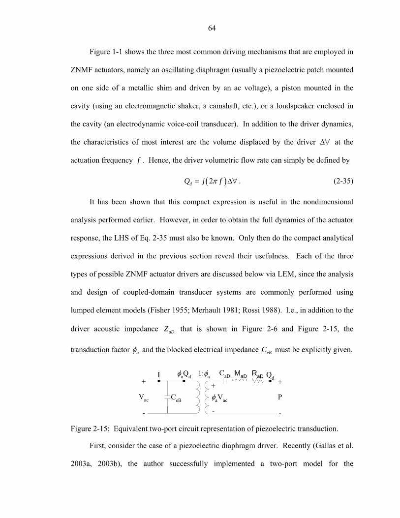
64

Figure 1-1 shows the three most common driving mechanisms that are employed in

ZNMF actuators, namely an oscillating diaphragm (usually a piezoelectric patch mounted

on one side of a metallic shim and driven by an ac voltage), a piston mounted in the

cavity (using an electromagnetic shaker, a camshaft, etc.), or a loudspeaker enclosed in

the cavity (an electrodynamic voice-coil transducer). In addition to the driver dynamics,

the characteristics of most interest are the volume displaced by the driver ∆∀ at the

actuation frequency f . Hence, the driver volumetric flow rate can simply be defined by

( )2dQ j fπ= ∆∀ . (2-35)

It has been shown that this compact expression is useful in the nondimensional

analysis performed earlier. However, in order to obtain the full dynamics of the actuator

response, the LHS of Eq. 2-35 must also be known. Only then do the compact analytical

expressions derived in the previous section reveal their usefulness. Each of the three

types of possible ZNMF actuator drivers are discussed below via LEM, since the analysis

and design of coupled-domain transducer systems are commonly performed using

lumped element models (Fisher 1955; Merhault 1981; Rossi 1988). I.e., in addition to the

driver acoustic impedance aDZ that is shown in Figure 2-6 and Figure 2-15, the

transduction factor aφ and the blocked electrical impedance eBC must be explicitly given.

+

-

Vac

+

-

P

I QdφaQd

φaVac

+

-

CeB

1:φa CaD RaDMaD

Figure 2-15: Equivalent two-port circuit representation of piezoelectric transduction.

First, consider the case of a piezoelectric diaphragm driver. Recently (Gallas et al.

2003a, 2003b), the author successfully implemented a two-port model for the

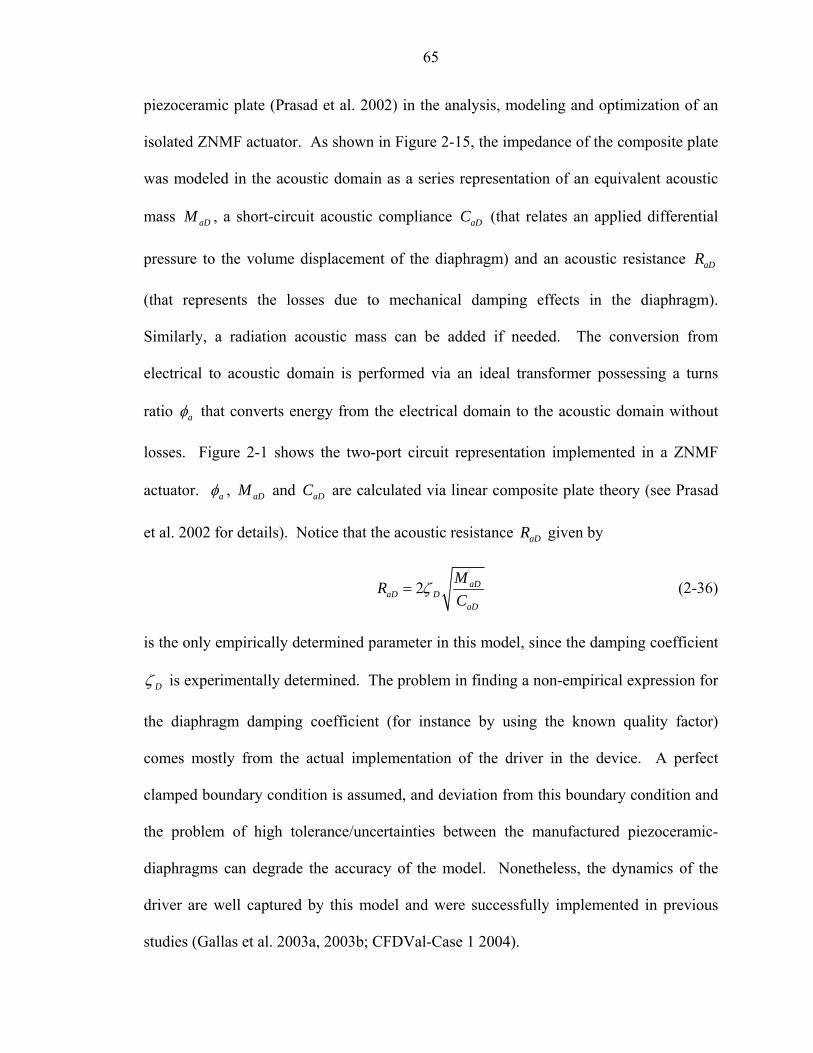
65

piezoceramic plate (Prasad et al. 2002) in the analysis, modeling and optimization of an

isolated ZNMF actuator. As shown in Figure 2-15, the impedance of the composite plate

was modeled in the acoustic domain as a series representation of an equivalent acoustic

mass aDM , a short-circuit acoustic compliance aDC (that relates an applied differential

pressure to the volume displacement of the diaphragm) and an acoustic resistance aDR

(that represents the losses due to mechanical damping effects in the diaphragm).

Similarly, a radiation acoustic mass can be added if needed. The conversion from

electrical to acoustic domain is performed via an ideal transformer possessing a turns

ratio aφ that converts energy from the electrical domain to the acoustic domain without

losses. Figure 2-1 shows the two-port circuit representation implemented in a ZNMF

actuator. aφ , aDM and aDC are calculated via linear composite plate theory (see Prasad

et al. 2002 for details). Notice that the acoustic resistance aDR given by

2 aDaD D

aD

MRC

ζ= (2-36)

is the only empirically determined parameter in this model, since the damping coefficient

Dζ is experimentally determined. The problem in finding a non-empirical expression for

the diaphragm damping coefficient (for instance by using the known quality factor)

comes mostly from the actual implementation of the driver in the device. A perfect

clamped boundary condition is assumed, and deviation from this boundary condition and

the problem of high tolerance/uncertainties between the manufactured piezoceramic-

diaphragms can degrade the accuracy of the model. Nonetheless, the dynamics of the

driver are well captured by this model and were successfully implemented in previous

studies (Gallas et al. 2003a, 2003b; CFDVal-Case 1 2004).

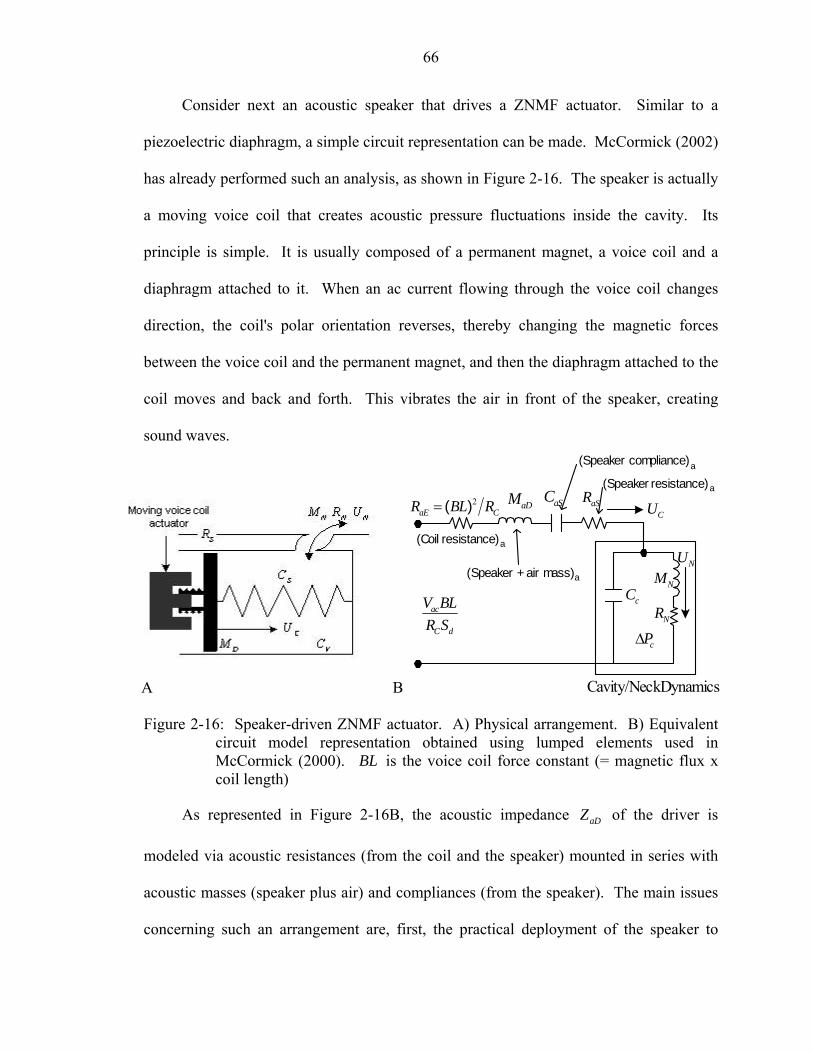
66

ac

C d

V BLR S

aSC2aE CR BL R= ( ) aSR

CU

cP∆

NM

NRcC

NU

Cavity/Neck Dynamics

aDM

(Coil resistance)a

(Speaker + air mass)a

(Speaker compliance)a

(Speaker resistance)a

Consider next an acoustic speaker that drives a ZNMF actuator. Similar to a

piezoelectric diaphragm, a simple circuit representation can be made. McCormick (2002)

has already performed such an analysis, as shown in Figure 2-16. The speaker is actually

a moving voice coil that creates acoustic pressure fluctuations inside the cavity. Its

principle is simple. It is usually composed of a permanent magnet, a voice coil and a

diaphragm attached to it. When an ac current flowing through the voice coil changes

direction, the coil's polar orientation reverses, thereby changing the magnetic forces

between the voice coil and the permanent magnet, and then the diaphragm attached to the

coil moves and back and forth. This vibrates the air in front of the speaker, creating

sound waves.

Figure 2-16: Speaker-driven ZNMF actuator. A) Physical arrangement. B) Equivalent

circuit model representation obtained using lumped elements used in McCormick (2000). BL is the voice coil force constant (= magnetic flux x coil length)

As represented in Figure 2-16B, the acoustic impedance aDZ of the driver is

modeled via acoustic resistances (from the coil and the speaker) mounted in series with

acoustic masses (speaker plus air) and compliances (from the speaker). The main issues

concerning such an arrangement are, first, the practical deployment of the speaker to

A B

67

drive the ZNMF actuator in a desired frequency range. Also, a loudspeaker creates

pressure fluctuations whose characteristics (amplitude and frequency) depend on the

speaker dynamics. For example, if the speaker is mounted in a large cavity enclosure

(whose size is greater than the acoustic wavelength), it might excite the acoustic modes

of the cavity, thereby resulting in three-dimensionality of the flow in the slot.

sealingmembrane

shaker

bottomcavity

cavity

orifice ventchannel

Figure 2-17: Schematic of a shaker-driven ZNMF actuator, showing the vent channel between the two sealed cavities.

Finally, consider a piston-like driver. It could be operated either mechanically, for

instance by a camshaft or by other mechanical means, or by using an electromagnetic

shaker. Here, we turn our attention to the latter application. An electromagnetic piston

usually consists of a moving voice coil shaft that drives a rigid piston plate and, in

essence, follows the same concept as presented above for the case of a voice coil

loudspeaker. Although the previous discussion on the LEM representation remains the

same here, the major difference comes from the nature of the piston itself. In fact, while

the top face of the piston is facing the cavity of the ZNMF actuator, another cavity on the

opposite side of the piston is present, as shown in Figure 2-17. This cavity may or may

not be vented to the other cavity. If sealed, when the ZNMF device is running at a

specific condition, an additional pressure load is created on the piston plate to account for

the static pressure difference between the cavities that may deteriorate the nominal

transducer performance. To alleviate this effect, the ZNMF cavity and the bottom cavity

68

could be vented together, in a similar manner to that employed for a microphone design.

Also, this bottom cavity should be added in series with the ZNMF cavity (since they

share the same common flow) in the circuit representation of the actuator that is shown in

Figure 2-18.

Qd( ) :1BL

eU

Z aC

Qd-Qv-Qj

Qj

Z aO

∆Pc

electromagnetic moving-coil transducer

electrodynamic coupling

electricalsource

Z aC b

ot

Z aVen

t

Qv

Figure 2-18: Circuit representation of a shaker-driven ZNMF actuator, where aCZ is the

acoustic impedance of the ZNMF cavity, botaCZ is the acoustic impedance of the bottom cavity, and aVentZ is the acoustic impedance of the vent channel.

Even though tools are available using lumped element modeling, the ZNMF

actuator driver must be modeled with care, especially when deployed in a physical

apparatus. However, once the driver dynamics have been successfully modeled, its

implementation in the dimensionless analytical expressions derived in this chapter can

yield powerful insight into the analysis and the design of a ZNMF actuator. This method

can then be extended by including the effect of an external boundary layer, as shown in

Chapter 7.

Now that some insight has been gained on the dynamics of a ZNMF actuator in still

air, a test matrix is constructed to carefully investigate both experimentally and

numerically the unresolved features of these types of devices, especially on refining the

nonlinear loss coefficient of the orifice.

69

Test Matrix

A significant database forms the basis of a test matrix that includes direct numerical

simulations and experimental results. The test matrix is comprised of various test

actuator configurations that are examined to ultimately assess the accuracy of the

developed reduced-order models over a wide range of operating conditions.

The goal is to test various actuator configurations in order to cover a wide range of

operating conditions, in a quiescent medium, by varying the key dimensionless

parameters extracted in the above dimensional analysis. Available numerical simulations

are used along with experimental data performed in the Fluid Mechanics Laboratory at

the University of Florida on a single piezoelectric-driven ZNMF device exhausting in still

air. Table 2-3 describes the test matrix. The first six cases are direct numerical

simulations (DNS) from the George Washington University under the supervision of

Prof. Mittal. They use a 2D DNS simulation whose methodology is detailed in Appendix

F. Case 8 comes from the first test case of the NASA LaRC workshop (CFDVal 2004).

Then, Case 9 to Case 72 are experimental test cases performed at the University of

Florida for axisymmetric piezoelectric-driven ZNMF actuators. The experimental setup

is described in details in Chapter 3, and the results are systematically analyzed and

studied in Chapter 4, Chapter 5, and Chapter 6.

Table 2-3: Test matrix for ZNMF actuator in quiescent medium

Case Type f (Hz) d (mm)

h (mm) w/d ∀

(mm3) S Re St f/fH f/fd Jet

1 CFD 0.38 1 1 ∞ 800 25.0 262 2.4 0.13 — X 2 CFD 0.38 1 2 ∞ 800 25.0 262 2.4 0.15 — X 3 CFD 0.06 1 0.68 ∞ 360 10.0 262 0.4 0.01 — J 4 CFD 0.20 0.1 0.1 ∞ 800 5.0 63.6 0.4 0.00 — J 5 CFD 0.80 0.1 0.1 ∞ 800 10.0 255 0.4 0.01 — J 6 CFD 1.99 0.1 0.1 ∞ 800 15.8 477 0.5 0.03 — J 7 CFD 1.99 0.1 0.1 ∞ 800 15.8 636 0.4 0.03 — J 8 exp/cfd 446 1.27 13.5 28 7549 17.1 861 0.3 2.65 0.99 J 9 exp. 39 1.9 1.8 — 7109 7.6 8.79 6.6 0.06 0.06 X

70


h (mm) w/d ∀


10 exp. 39 1.9 1.8 — 7109 7.6 12.0 4.8 0.06 0.06 J 11 exp. 39 1.9 1.8 — 7109 7.6 22.6 2.5 0.06 0.06 J 12 exp. 39 1.9 1.8 — 7109 7.6 33.2 1.7 0.06 0.06 J 13 exp. 39 1.9 1.8 — 7109 7.6 39.8 1.4 0.06 0.06 J 14 exp. 39 1.9 1.8 — 7109 7.6 46.5 1.2 0.06 0.06 J 15 exp. 39 1.9 1.8 — 7109 7.6 52.5 1.1 0.06 0.06 J 16 exp. 39 1.9 1.8 — 7109 7.6 59.7 1.0 0.06 0.06 J 17 exp. 39 1.9 1.8 — 7109 7.6 66.0 0.9 0.06 0.06 J 18 exp. 39 1.9 1.8 — 7109 7.6 73.7 0.8 0.06 0.06 J 19 exp. 39 1.9 1.8 — 7109 7.6 81.6 0.7 0.06 0.06 J 20 exp. 39 1.9 1.8 — 7109 7.6 88.2 0.6 0.06 0.06 J 21 exp. 780 1.9 1.8 — 7109 34.0 192 6.0 1.24 1.23 X 22 exp. 780 1.9 1.8 — 7109 34.0 242 4.8 1.24 1.23 J 23 exp. 780 1.9 1.8 — 7109 34.0 374 3.1 1.24 1.23 J 24 exp. 780 1.9 1.8 — 7109 34.0 513 2.2 1.24 1.23 J 25 exp. 780 1.9 1.8 — 7109 34.0 637 1.8 1.24 1.23 J 26 exp. 780 1.9 1.8 — 7109 34.0 750 1.5 1.24 1.23 J 27 exp. 780 1.9 1.8 — 7109 34.0 825 1.4 1.24 1.23 J 28 exp. 780 1.9 1.8 — 7109 34.0 930 1.2 1.24 1.23 J 29 exp. 780 1.9 1.8 — 7109 34.0 1131 1.1 1.24 1.23 J 30 exp. 780 1.9 1.8 — 7109 34.0 1120 1.0 1.24 1.23 J 31 exp. 780 1.9 1.8 — 7109 34.0 1200 1.0 1.24 1.23 J 32 exp. 780 1.9 1.8 — 7109 34.0 1264 0.9 1.24 1.23 J 33 exp. 780 1.9 1.8 — 7109 34.0 1510 0.8 1.24 1.23 J 34 exp. 780 1.9 1.8 — 7109 34.0 1589 0.7 1.24 1.23 J 35 exp. 780 1.9 1.8 — 7109 34.0 1683 0.7 1.24 1.23 J 36 exp. 780 1.9 1.8 — 7109 34.0 1774 0.6 1.24 1.23 J 37 exp. 780 1.9 1.8 — 7109 34.0 1842 0.6 1.24 1.23 J 38 exp. 780 1.9 1.8 — 7109 34.0 1876 0.6 1.24 1.23 J 39 exp. 780 1.9 1.8 — 7109 34.0 2755 0.4 1.24 1.23 J 40 exp. 1200 1.9 1.8 — 7109 42.1 90.8 19.5 1.91 1.90 X 41 exp. 39 2.98 1.05 — 7109 11.9 40.6 3.49 0.04 0.06 J 42 exp. 39 2.98 1.05 — 7109 11.9 47.3 2.99 0.04 0.06 J 43 exp. 39 2.98 1.05 — 7109 11.9 63.4 2.23 0.04 0.06 J 44 exp. 500 2.98 1.05 — 7109 42.6 1959 0.93 0.55 0.79 J 45 exp. 500 2.98 1.05 — 7109 42.6 2615 0.69 0.55 0.79 J 46 exp. 780 2.98 1.05 — 7109 53.2 109 26.0 0.86 1.23 X 47 exp. 780 2.98 1.05 — 7109 53.2 254 11.2 0.86 1.23 X 48 exp. 780 2.98 1.05 — 7109 53.2 571 4.96 0.86 1.23 J 49 exp. 780 2.98 1.05 — 7109 53.2 1439 1.97 0.86 1.23 J 50 exp. 780 2.98 1.05 — 7109 53.2 2022 1.40 0.86 1.23 J 51 exp. 39 2.96 4.99 — 7109 11.8 29.8 4.69 0.06 0.06 J 52 exp. 39 2.96 4.99 — 7109 11.8 43.0 3.25 0.06 0.06 J 53 exp. 39 2.96 4.99 — 7109 11.8 55.7 2.51 0.06 0.06 J 54 exp. 39 2.96 4.99 — 7109 11.8 71.9 1.94 0.06 0.06 J 55 exp. 780 2.96 4.99 — 7109 52.9 125 22.3 1.25 1.23 X 56 exp. 780 2.96 4.99 — 7109 52.9 318 8.79 1.25 1.23 X 57 exp. 780 2.96 4.99 — 7109 52.9 867 3.22 1.25 1.23 J 58 exp. 780 2.96 4.99 — 7109 52.9 2059 1.36 1.25 1.23 J 59 exp. 780 2.96 4.99 — 7109 52.9 3039 0.92 1.25 1.23 J

71


h (mm) w/d ∀


60 exp. 39 1.0 5.0 — 7109 4.0 132 0.12 0.16 0.06 J 61 exp. 39 1.0 5.0 — 7109 4.0 157 0.10 0.16 0.06 J 62 exp. 39 1.0 5.0 — 7109 4.0 205 0.08 0.16 0.06 J 63 exp. 500 1.0 5.0 — 7109 14.3 286 0.72 2.10 0.79 J 64 exp. 500 1.0 5.0 — 7109 14.3 461 0.44 2.10 0.79 J 65 exp. 730 1.0 5.0 — 7109 17.3 269 1.11 3.07 1.16 J 66 exp. 730 1.0 5.0 — 7109 17.3 611 0.49 3.07 1.16 J 67 exp. 730 1.0 5.0 — 7109 17.3 893 0.33 3.07 1.16 J 68 exp. 730 1.0 5.0 — 7109 17.3 1081 0.28 3.07 1.16 J 69 exp. 730 1.0 5.0 — 7109 17.3 1361 0.22 3.07 1.16 J 70 exp. 39 0.98 0.92 — 7109 3.9 49.6 0.31 0.09 0.06 J 71 exp. 39 0.98 0.92 — 7109 3.9 112 0.14 0.09 0.06 J 72 exp. 39 0.98 0.92 — 7109 3.9 179 0.09 0.09 0.06 J

To conclude this chapter, the existing lumped element model from Gallas et al.

(2003a) has been presented and reviewed, and it has been shown that it could be extended

to more general device configurations, particularly in terms of orifice geometry and

driver configuration. Then, a dimensional analysis of an isolated ZNMF actuator was

performed. A compact expression, in terms of the principal dimensionless parameters,

was found for the nondimensional linear transfer function that relates the output to the

input of the actuator, regardless of the orifice geometry and of the driver configuration.

Next, some modeling issues have been investigated for the different components of a

ZNMF actuator. Specifically, the LEM technique has been used in the time domain to

yield some insight on the orifice shape effect, and a physical description on the associated

orifice losses has been provided. Finally, since one of the goals of this research is to

develop a refined low-order model, which is presented in Chapter 6 and that builds on the

results presented in the subsequent chapters, a significant database forms the basis of a

test matrix that is comprised of direct numerical simulations and experimental results.

72

CHAPTER 3

EXPERIMENTAL SETUP

This chapter provides the details on the design and the specifications of the ZNMF

devices used in the experimental study. Descriptions of the cavity pressure, driver

deflection, and actuator exit velocity measurements are provided, along with the dynamic

data acquisition system employed. Then, the data reduction process is presented with

some general results. A description of the Fourier series decomposition applied to the

phase-locked, ensemble average time signals is presented next. Finally, a description of

the flow visualization technique employed to determine if a synthetic jet is formed is then

provided.

Experimental Setup

In this dissertation, two different experiments are performed. The first one,

referred to as Test 1, is used in the orifice flow analysis presented in Chapter 4 and the

corresponding test cases are listed in Table 2-3. The second test, Test 2, is used in the

cavity compressibility analysis (presented in Chapter 5). Test 1 consists of phase-locked

measurements of the velocity profile at the orifice, cavity pressure, and diaphragm

deflection, and the device uses a large diaphragm and has an axisymmetric straight

orifice. On the other hand, in Test 2 only the frequency response of the centerline

velocity and driver displacement are acquired, and the device uses a small diaphragm and

the orifice is a rectangular slot. However, since the two tests share the same equipment

and basic setup and Test 1 requires additional equipment, only Test 1 is detailed below.

73

PMTs colorseparator

bellowsextender

200 mmmicro lens

to processor

syntheticjet Z

Y

3 componenttraverse

X

Y

X

Z

probe

from laser

Side View

Top View

to processor

mic 1

displacement sensor

piezoelectricdiaphragm

mic 2

Figure 3-1: Schematic of the experimental setup for phase-locked cavity pressure,

diaphragm deflection and off-axis, two-component LDV measurements.

diaphragmmount

body platetop plate clamp plate

orifice plate

d

h

cavity ( )∀

diaphragm(φ = 37 mm)

+-

Figure 3-2: Exploded view of the modular piezoelectric-driven ZNMF actuator used in

the experimental test.

74

Figure 3-1 shows a schematic of the complete experimental setup, where a large

enclosure ( )2 1 1m m m× × is constructed with a tarp to house the ZNMF actuator device,

the LDV transmitting and receiving optics, and the displacement sensor. The ZNMF

actuator consists of a piezoelectric diaphragm driver mounted on the side of the cavity,

and has an axisymmetric straight orifice. The commercially available diaphragm (APC

International Ltd. Model APC 850) consists of a piezoelectric patch (PZT 5A) which is

bonded to a metallic shim (made of brass). The diaphragm is clamped between two

plates and have an effective diameter equals to 37 mm. Figure 3-2 gives an exploded

view of the device and Table 3-1 summarizes the geometric dimensions.

Only the orifice top plate is changed to allow five orifice aspect ratio

configurations, and the input voltage and actuation frequency are also varied to yield a

large parameter space investigation in terms of the following dimensional parameters:

3; ;Re; ; ; ;H dh d S kd dω ω ω ω ∆∀ . An emphasis is made in the orifice aspect ratio

variation, hence the five different orifices used, and the input sinusoidal voltage applied

to the driver varies from 4 Vpp to 60 Vpp, the frequencies being set to 39, 500, 730 and

780 Hz. This device is constructed specifically to operate in the low-to-moderate Stokes

number range, 60S < . The signal source is provided by an Agilent model 33120A

function generator. The signal from the function generator is applied to a Trek amplifier

(model 50/750), and the amplified sinusoidal input voltage signal is then applied to the

driver via a small wire soldered to the piezoceramic patch, which converts the voltage

into a mechanical deflection.

Since the two variable input parameters are the frequency of oscillation, the

amplitude of the forcing signal, and the different orifice plates, the change in these

75

dimensional parameters can be converted into a change in dimensionless numbers like the

Stokes number S, the actuation-to-Helmholtz frequency ratio Hf f , the driving-to-

diaphragm natural frequency df f , the dimensionless wavenumber kd , and the

dimensionless driver amplitude 3d∆∀ .

Table 3-1: ZNMF device characteristic dimensions used in Test 1 Cavity Volume ∀ (m3) 7.11×10-6 Orifice Diameter d (mm) 1.0 2.0 3.0 1.0 1.0 Height h (mm) 5.0 1.8 1.0 0.9 5.0 Piezoelectric diaphragm Shim (Brass) Elastic modulus (Pa) 8.963×1010 Poisson’s ratio 0.324 Density (kg/m3) 8700 Thickness (mm) 0.10 Diameter (mm) 37 Piezoceramic (PZT-5A) Elastic modulus (Pa) 6.3×1010 Poisson’s ratio 0.31 Density (kg/m3) 7700 Thickness (mm) 0.11 Diameter (mm) 25 Relative dielectric constant 1750 d31 (m/V) -1.75×10-10 Cef (nF) 76

Cavity Pressure

The pressure fluctuations inside the cavity are measured simultaneously at two

locations using flush-mounted Brüel and Kjær (B&K) 1 8′′ diameter condenser type

microphones (Model 4138) powered by B&K 2670 pre-amplifiers and a B&K 2804

power supply. Before each test, the microphones are calibrated using a B&K

pistonphone type 4228. The operational frequencies of the ZNMF device are usually

from about 30 Hz to 1 kHz in this test, which is well within the frequency range of the

76

microphone, from 6.5 Hz to 140 kHz (± 2 dB). The nominal sensitivity of the B&K 4138

type microphones is 60 1.5− ± dB (ref. 1V/Pa), or 1.0 mV/Pa. When assembling the

device parts together, all leaks are carefully minimized by sealing the parts with RTV,

and the pressure ports are properly sealed. Figure 3-3 shows a schematic of the two

microphone measurement locations inside the cavity. Notice that for the highest

frequency of operation (780 Hz), the ratio of the wavelength ( )0 2c f kλ π= = to the

distance ( )28.7l mm= separating the two microphones in the cavity is less than unity

( )0.41kl < , implying that the acoustic pressure waves inside the cavity change very little

because the distance between microphones is small compared with the acoustic

wavelength.

12.5 mm

28.7 mm

37.0 mm

Mic 1

Mic 2

3.6 mmOrifice

Diaphragm

18.5 mm

22.7 mm

Figure 3-3: Schematic (to scale) of the location of the two 1 8′′ microphones inside the

ZNMF actuator cavity.

Diaphragm Deflection

The deflection of the diaphragm is measured using a laser displacement sensor

Micro-Epsilon Model ILD2000-10. The sensitivity is 1 V/mm, with a full-scale range of

10 mm and a resolution of ~0.1 µm. The sensor bandwidth is 10 kHz, and the spot size

of the laser is 40 µm. Figure 3-4 gives the displacement sensor sign convention between

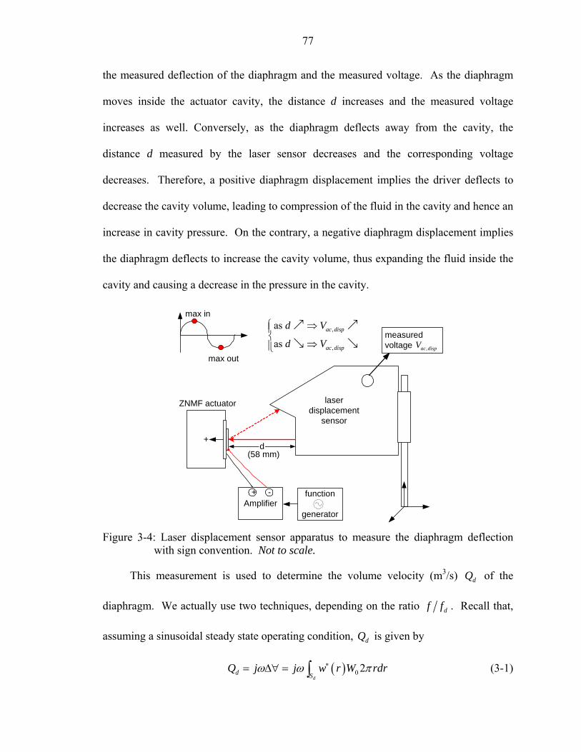
77

the measured deflection of the diaphragm and the measured voltage. As the diaphragm

moves inside the actuator cavity, the distance d increases and the measured voltage

increases as well. Conversely, as the diaphragm deflects away from the cavity, the

distance d measured by the laser sensor decreases and the corresponding voltage

decreases. Therefore, a positive diaphragm displacement implies the driver deflects to

decrease the cavity volume, leading to compression of the fluid in the cavity and hence an

increase in cavity pressure. On the contrary, a negative diaphragm displacement implies

the diaphragm deflects to increase the cavity volume, thus expanding the fluid inside the

cavity and causing a decrease in the pressure in the cavity.

Amplifier

+

laserdisplacement

sensor

ZNMF actuator

measuredvoltage

,

,

as

as ac disp

ac disp

d V

d V

⎧ ⇒⎪⎨

⇒⎪⎩ ,ac dispV

max in

max out

(58 mm)

function

generator

+ -

d

Figure 3-4: Laser displacement sensor apparatus to measure the diaphragm deflection

with sign convention. Not to scale.

This measurement is used to determine the volume velocity (m3/s) dQ of the

diaphragm. We actually use two techniques, depending on the ratio df f . Recall that,

assuming a sinusoidal steady state operating condition, dQ is given by

( ) 0 2d

d SQ j j w r W rdrω ω π∗= ∆∀ = ∫ (3-1)

78

where ( ) ( ) 0w r w r W∗ = is the transverse displacement of the diaphragm normalized by

the centerline amplitude 0W . Therefore, if one knows the diaphragm mode shape, then

only 0W is required via measurement to calculate dQ by virtue of Eq. 3-1. If the mode

shape is not known, then it must also be measured. The former technique is thus a single-

point measurement, where only the centerline displacement of the oscillating diaphragm

is acquired phased-locked to the drive signal. The mode shape is computed using the

static linear composite plate theory described in Prasad et al. (2002). This model is only

valid from frequencies ranging from DC up to the first natural frequency df , hence the

importance of the frequency ratio df f . This piezoelectric diaphragm has its first

natural frequency at about 632df Hz . Then from Eq. 3-1, the diaphragm volume flow

rate can be determined by simply integrating the mode shape of the circular piezoelectric

diaphragm.

In the case where the frequency ratio df f is greater than one, the static mode

shape is no longer valid, so a second measurement technique is employed to

experimentally acquire the mode shape by systematically traversing the laser

displacement sensor across the diaphragm radius. The root-mean-square value of the

diaphragm deflection is computed for each position, and assuming a sinusoidal signal the

amplitude is obtained by multiplying the rms value by a factor 2 . This sinusoidal

assumption was visually checked during the time of acquisition for all signals, and on

some test cases a Fourier series decomposition was performed that validated this

assumption, as described at the end of this Chapter. Figure 3-5 shows the measured and

computed mode shape of the piezoelectric diaphragm at several forcing frequencies. In

79

the case where 1df f ≤ , the comparison between the experimentally determined mode

shape and the linear model shows good agreement. Similarly, the figure shows the

diaphragm deflection along versus radius for the highest frequency used in this

experimental test, 780f Hz= , which clearly indicates the breakdown of the static model.

The slope discontinuity in the experimental data near the position 0.65r a = corresponds

to the edge of the piezoelectric patch that is bonded via epoxy on the metallic shim and is

a result of optical diffraction of the laser beam at this location.

0 0.2 0.4 0.6 0.8 10

0.01

0.02

0.03

0.04

0.05

0.06

normalized radius

mag

nitu

de (m

m)

exp. datalinear mode shape

f/fd=0.79

f/fd=0.06

f/fd=1.23

Figure 3-5: Diaphragm mode shape comparison between linear model and experimental

data at three test conditions: 0.06df f = and pp60 VacV = , 0.79df f = and

pp50 VacV = , and 1.23df f = and pp20 VacV = .

Velocity Measurement

Velocity measurements of the flowfield emanating from the ZNMF orifice are

obtained using Laser Doppler Velocimetry (LDV), the details of which are listed in Table

3-2. The synthetic jet actuator is mounted to a three-axis traverse with sub-micron spatial

resolution to move the orifice with respect to the fixed laser probe volume location. The

80

traverse is traversed in either 0.1 mm or 0.05 mm steps across the orifice, yielding a total

of 31 to 41 positions at which the phase-locked velocities are measured, depending on the

orifice diameter.

The enclosure shown in Figure 3-1 is seeded with LeMaitre haze fluid using a

LeMaitre Neutron XS haze machine, where the haze particles have a mean diameter

small enough that it does not influence on the measured flow field (this is verified by

computing the time constant τ of the particle and then by showing that the particle

response, which is like a 1st-order system, faithfully tracks velocity fluctuations at

frequencies well below 1 τ . The reader is referred to Holman (2005) for the details and

analysis on the seed particle dynamics).

Probe

Combined 514.5 nm488 nm beams

Separate 514.5 nmand 488 nm beams inthe horizontal plane

LDV 1LDV 2

Syntheticjet actuator

v

u

(front view)(side view)

Figure 3-6: LDV 3-beam optical configuration.

The 488 and 514.5 nm wavelengths of a Spectra-Physics 2020 argon-ion laser are

used to obtain coincident, two-component velocity measurements using a Dantec

FiberFlow system Typically, the beam strength is approximately 30 ~ 50 mW for the

green (514.5 nm) and 15 ~ 20 mW for the blue (488 nm). As shown in Figure 3-6, a

three-beam optical combiner configuration is used to facilitate velocity measurements at

81

the exit plane surface of the synthetic jet actuator. Due to mounting constraints, the

actuator is mounted at a 45o angle with respect to the horizontal such that the scattered

light from the probe volume may reach the receiving optics. A direction cosine

transformation is then applied to the acquired velocity components LDV 1 and LDV 2 to

extract the axial and radial velocity components.

A 200 mm micro lens and bellows extender collects lights at 90º off-axis in order to

improve the spatial resolution since only a slice of the probe volume is “seen” by the

optics. Scattered light from the probe volume is focused and passed through a 100 µm

diameter pinhole aperture. The resulting field of view was imaged using a micro-ruler

and found to be approximately 10 µm, indicating that the effective length of the probe

volume dz has been reduced by over an order of magnitude from that listed in Table 3-2.

After the pinhole, a color separator splits the 514.5 nm and 488 nm wavelengths and

transmits the light to two separate photomultiplier tubes (PMTs), which convert the

Doppler signal to a voltage, and it is then passed through a high-pass filter to remove the

Doppler pedestal. An additional band-pass filter is then applied to remove noise in the

signal outside of the expected velocity range. Next, the FFT of the signals is computed,

and the velocity is then computed from the measured Doppler frequency and the fringe

spacing. Finally, since two components of velocity are measured, a coincidence filter is

applied to ensure that a Doppler signal is present on both channels at the same instant in

time. At each radial measurement position, 8192 samples are acquired in both LDV1 and

LDV2, which yields approximately 200 velocity values at each phase bin. Note that each

data point has a time of arrival relative to the trigger signal that denotes the zero phase

82

angle. The LDV data are then divided into phase bins with 15o spacing, as explained in

more details in the data processing section.

Table 3-2: LDV measurement details Property LDV 1 LDV 2 Wavelength (nm) 514.5 488 Focal length (mm) 120 120 Beam diameter (mm) 1.35 1.35 Beam spacing (mm) 26.9 26.9 Number of fringes 25 25 Fringe spacing (µm) 2.31 2.19 Beam half-angle (deg) 6.39 6.39 Probe volume – dx (mm) 0.058 0.056 Probe volume – dy (mm) 0.058 0.055 Probe volume – dz (mm) 0.523 0.496

Data-Acquisition System

Figure 3-7 shows a flow chart of the experimental setup. The piezoelectric

diaphragm is actuated using an Agilent 33120A function generator with a Trek amplifier

(Model 50/750). Using the sync signal of the function generator, the measured quantities

are acquired in a phase-locked mode. A National Instruments model NI-4552 dynamic

signal analyzer (DSA) PCI card is used for data acquisition (DAQ). It is a 16-bit, sigma-

delta DAQ card that can sample up to 4 channels of analog input simultaneously and has

a bandwidth of approximately 200 kHz. In addition, a built-in analog and digital anti-

aliasing filter is used. The low-pass analog filter has a fixed cutoff frequency of 4 MHz,

which is well above the frequencies considered here and may be considered to have zero

phase offset in the passband. The digital filter removes all frequency components above

the desired Nyquist frequency in the oversampled signal and then decimates the resulting

signal to achieve the desired sampling rate.

Similarly, since the signals are ac coupled to remove any dc offset and to increase

the resolution in the signal measurements, any slight amplitude attenuation and phase

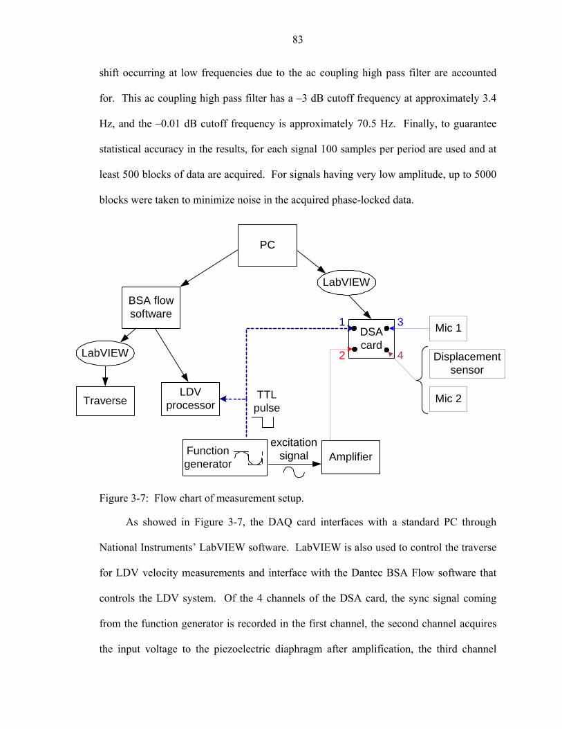
83

shift occurring at low frequencies due to the ac coupling high pass filter are accounted

for. This ac coupling high pass filter has a –3 dB cutoff frequency at approximately 3.4

Hz, and the –0.01 dB cutoff frequency is approximately 70.5 Hz. Finally, to guarantee

statistical accuracy in the results, for each signal 100 samples per period are used and at

least 500 blocks of data are acquired. For signals having very low amplitude, up to 5000

blocks were taken to minimize noise in the acquired phase-locked data.

PC

BSA flowsoftware

LDVprocessor

LabVIEW

Traverse

LabVIEW

Amplifier

TTLpulse

DSAcard

Mic 1

Displacementsensor

Mic 2

1

2

3

4

Functiongenerator

excitationsignal

Figure 3-7: Flow chart of measurement setup.

As showed in Figure 3-7, the DAQ card interfaces with a standard PC through

National Instruments’ LabVIEW software. LabVIEW is also used to control the traverse

for LDV velocity measurements and interface with the Dantec BSA Flow software that

controls the LDV system. Of the 4 channels of the DSA card, the sync signal coming

from the function generator is recorded in the first channel, the second channel acquires

the input voltage to the piezoelectric diaphragm after amplification, the third channel

84

monitors the pressure fluctuations from microphone 1 situated at the bottom of the cavity,

and the fourth channel acquires either the signal from the displacement sensor or from the

second microphone located in the side of the cavity.

0 45 90 135 180 225 270 315 360

-1

-0.8

-0.6

-0.4

-0.2

0

0.2

0.4

0.6

0.8

1

phase

Nor

mal

ized

qua

ntiti

es

0 45 9

-1

-0.8

-0.6

-0.4

-0.2

0

0.2

0.4

0.6

0.8

1

Nor

mal

ized

qua

ntiti

es

Figure 3-8: Phase-locked signalstrigger signal, displaceCase 70, f = 39 Hz. B)

df f<

A

df f>

B

input signal trigger signal diaph disp Mic 1 Mic 2

input signal trigger signal diaph disp Mic 1 Mic 2

0 135 180 225 270 315 360phase

acquired from the DSA card, showing the normalized ment signal, pressure signals and excitation signal. A) Case 65, f = 730 Hz.

85

Two sample graphs of the trigger signal, displacement signal, pressure signals and

excitation waveform coming from the DSA card during one cycle are shown in Figure

3-8. Figure 3-8A is representative of a test case in which the driving signal frequency is

below the resonance frequency of the diaphragm df , and it can be seen that the

diaphragm displacement is out of phase with the input voltage. On the other hand, when

the device is actuated beyond df , a 180o phase shift occurs in the diaphragm frequency

response, hence the input signal and the displacement signal are nearly in phase, as

shown in Figure 3-8B. Similarly, this means that a positive voltage from the function

generator results in a diaphragm deflection out from the cavity. Note that this is a

relevant observation when comparing the experimental results with the low-dimensional

model discussed in later chapters. The dynamics of the diaphragm can also be seen from

Figure 3-8 as it deflects in and out of the cavity. An increase in the diaphragm deflection

results in a rise in cavity pressure (with a phase lag), and vice versa, which confirms the

sign convention shown previously in Figure 3-4.

Data Processing

Once the data have been simultaneously acquired for the cavity pressures,

diaphragm displacement, and the velocity profile from the setup described above, it then

needs to be carefully processed in order to have great confidence in using the results.

First, the pressure and diaphragm signals are averaged using a vector spectral averaging

technique to eliminate noise from the synchronous signals. This averaging technique, in

contrast with the more common RMS averaging technique that reduces signal

fluctuations but not the noise floor, computes the average of complex quantities directly,

separating the real from the imaginary part, which then reduces the noise floor since

86

random signals are not phase-coherent from one data block to the next. For instance,

using the vector averaging technique, the power spectrum is computed such that

(National Instruments 2000)

*G X X= ⋅ , (3-2)

where X is the complex FFT of a signal x, *X is the complex conjugate of X, and X is

the average of X, real and imaginary parts being averaged separately. In contrast, the

RMS averaging technique used the following equation for the power spectrum,

*G X X= ⋅ . (3-3)

Then, once the velocity data is acquired with the LDV system, the velocity profiles

must be integrated spatially and temporally to determine the average volume flow rate

jQ and hence jV , via

( )0

1 ,n

j n j nSQ v t x dtdS V S

τ

τ= =∫ ∫ , (3-4)

where 0 t τ< < is the time of expulsion portion of the cycle. However, an important

issue is statistical analysis of the LDV data. Velocity measurements “arrive” at random

points during a cycle, and like all experimental measurements, random noise also exists.

Therefore, the velocity data points must be sorted into phase bins to generate a

phase-locked velocity profile. Each bin is a representation of the mean and uncertainty

for all of the velocity points that fall within that bin. Therefore, to know the optimum bin

width to minimize the combined random and bias errors in the LDV measurements,

Figure 3-9 illustrates the percent error in the computed quantity jV from simulated LDA

data, for several simulated signal-to-noise ratios (SNR) and where 8192 samples are

87

acquired. As expected, for very large bin widths – on the order of 45o – the error in jV is

quite large. However, in the bin width range 5-20o, the error appears to be minimized. In

this plot, the mean value of the error is indicative of the bias error due to the size of the

bin width, while the error bars indicate the random error component. Not surprisingly, as

the SNR is increased, this random error decreases. Most notably, however, the optimum

phase bin width does not appear to be a function of the SNR. Based on this plot, an

acceptable trade-off in the experimental test is found by choosing a bin width of 15o,

which is equivalent to sampling 24 points per period.

0 10 20 30 40 50-5

0

5

10

15

20

25

Bin width (deg)

Vj e

rror (

%)

SNR=0.5dBSNR=2dBSNR=8dBSNR=32dBSNR=128dB

Figure 3-9: Percentage error in jV from simulated LDV data at different signal to noise

ratio, using 8192 samples.

Next, an outlier rejection technique is applied on the raw velocity data to ensure

high quality experimental data. The modified Tau-Thomson outlier rejection criterion is

extended for two joint probability distribution function (pdf) distributions, corresponding

to the two set of data from LDV1 and LDV2, and a 99.9% confidence interval is retained.

Basically, the value of the joint pdf is computed for each data pair and is compared to a

88

look-up table that is generated depending on the percentage confidence interval from a

joint Gaussian pdf. This table gives the locus of points on the bounding ellipse and if a

point falls outside the ellipse, it is considered as an outlier. The details of this outlier

rejection criterion can be found in Holman (2005).

Another source of uncertainty comes from the phase resolution in each of the

signals. As seen above, the volume flow rate at the exit has a phase resolution of

15φ φ= °± ∆ , where φ∆ corresponds to half the bin width, i.e. 7.5º. Similarly, the data

acquired by the DSA card (trigger signal, diaphragm displacement and pressure

fluctuations) are acquired with 100 samples per period. That yields a phase uncertainty

of ±1.8º in these signals. Thus, the net uncertainty in the phase between the pressure and

the volume flow rate at the orifice is then estimated to be

,jQ Pφ φ δφ∆ = ∆ ± , (3-5)

where φ∆ is the phase difference in Qj and P∆ , and 7.5 1.8 9.4δφ = + = ° .

Next, the phase-locked profiles are spatially integrated to determine the periodic

volume flow rate since

( ) ( ),n

j nSQ t v t x dS= ∫ . (3-6)

The spatial integration is numerically performed using a trapezoidal integration

scheme. Figure 3-10 illustrates a set of typical phase-locked axial velocity profiles

during four different phases separated by 90º in the cycle, corresponding approximately

to maximum expulsion, maximum ingestion, and the two phases half way between.

Figure 3-10A plots the vertical velocity component, while the radial component is plotted

in Figure 3-10B, and Figure 3-10C gives the corresponding volume flow rate after

integration across the orifice. The error bars represent an estimate of the 95% confidence

89

interval for each velocity measurement and are obtained using a perturbation technique

(Schultz et al. 2005) that yields the same nominal values of uncertainty as a standard

Monte Carlo technique but with significantly less computational time.

Figure 3-10: Phase-locked velocity profiles and corresponding volume flow rate

acquired with LDV for Case 14 ( 8S = , pp28 VacV = , Re 46.5 3%= ± ), acquired at 0.05y d = . A) Vertical velocity component. B) Horizontal velocity component. C) Volume flow rate.

This method is employed to estimate the uncertainty in the averaged volume flow

rate. The 95% confidence interval estimate of jQ , in turn, is used to estimate the

-0.6 -0.4 -0.2 0 0.2 0.4 0.6-0.5

-0.4

-0.3

-0.2

-0.1

0

0.1

0.2

0.3

0.4

0.5

r/d

horizontal velocity u (m/s)

φ=0°φ=90°φ=180°φ=270°

-0.4 -0.2 0 0.2 0.4 0.6-0.8

-0.6

-0.4

-0.2

0

0.2

0.4

0.6

0.8

1

1.2

r/d

vertical velocity v (m/s)

φ=0°φ=90°φ=180°φ=270°

B

0 45 90 135 180 225 270 315 360-2

-1.5

-1

-0.5

0

0.5

1

1.5

2x 10

-6

Phase φ (deg)

Vol

ume

flow

rate

Qj (m

3 /s)

C

A

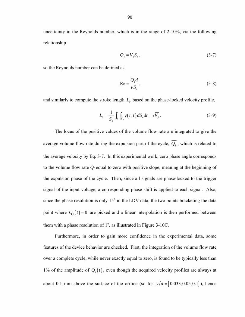
90

uncertainty in the Reynolds number, which is in the range of 2-10%, via the following

relationship

j j nQ V S= , (3-7)

so the Reynolds number can be defined as,

Re j

n

Q dSν

= , (3-8)

and similarly to compute the stroke length 0L based on the phase-locked velocity profile,

( )0 0

1 ,n

n jSn

L v r t dS dt VS

ττ= =∫ ∫ . (3-9)

The locus of the positive values of the volume flow rate are integrated to give the

average volume flow rate during the expulsion part of the cycle, jQ , which is related to

the average velocity by Eq. 3-7. In this experimental work, zero phase angle corresponds

to the volume flow rate Qj equal to zero with positive slope, meaning at the beginning of

the expulsion phase of the cycle. Then, since all signals are phase-locked to the trigger

signal of the input voltage, a corresponding phase shift is applied to each signal. Also,

since the phase resolution is only 15o in the LDV data, the two points bracketing the data

point where ( ) 0jQ t = are picked and a linear interpolation is then performed between

them with a phase resolution of 1o, as illustrated in Figure 3-10C.

Furthermore, in order to gain more confidence in the experimental data, some

features of the device behavior are checked. First, the integration of the volume flow rate

over a complete cycle, while never exactly equal to zero, is found to be typically less than

1% of the amplitude of ( )jQ t , even though the acquired velocity profiles are always at

about 0.1 mm above the surface of the orifice (so for [ ]0.033;0.05;0.1y d = ), hence

91

entraining some mass flow that could affect the volume flow rate. But this is not

surprising since a previous study has shown that a synthetic jet appears to remain zero-net

mass-flux even up to 0.4y d = (Smith and Glezer 1998); or actually as long as the

distance above the orifice is small compared to the stroke length ( )0y L .

Similarly for the cavity pressure measurements, the pressure signal sometimes is

“noisy” at the low frequency and low amplitude (or Reynolds number) cases, which is

principally due to 60 Hz line noise contamination. However, the signal is at least an

order of magnitude higher than the microphone noise floor, as shown in Figure 3-11 for

Case 52, and the Fourier series decomposition to the vector-averaged signal described

next still provides a good fit to the time signal, while rejecting contaminated noise.

0 45 90 135 180 225 270 315 360-2.5

-2

-1.5

-1

-0.5

0

0.5

1

1.5

2

2.5

phase

Pre

ssur

e (P

a)

noise floorpressure from microphone 1

Figure 3-11: Noise floor in the microphone measurements compared with Case 52.

Finally, repeatability in the extracted experimental data is an important issue to be

considered. Thus, to ensure fidelity in this experimental setup, several cases were retaken

at different periods in time. For instance, Case 20 and Case 29 have been experimentally

tested twice four months apart, while Case 62 and Case 69 have also been taken twice

92

within a time frame of weeks. Table 3-3 compares the results between these cases for the

principal governing parameters. As can be seen, the results are within the estimated

confidence interval. It should be pointed out though that for Case 20 and Case 29, the

velocity measurements were acquired at a slightly different distance from the surface

( 0.07y d = and 0.05y d = , respectively) that could explain the larger difference seen

in jQ in these cases.

Table 3-3: Repeatability in the experimental results cP∆ (Pa) Case # S Re

Mic 1 Mic 2 dQ (m3/s)

7.6 88.2 4%± 3.59 13%± 3.2 14%± 63.48 10 7%−× ± 20 7.6 85.0 4%± 3.26 10%± - 63.79 10 7%−× ± 33.9 1131 10%± 414.9 16%± 365.6 16%± 56.41 10 11%−× ± 29 33.9 968.8 6%± 331.5 10%± - 56.27 10 10%−× ± 3.9 204.9 4%± 39.9 11%± 43.0 12%± 64.09 10 6%−× ± 62 3.9 192.9 3%± 45.1 3%± 49.3 3%± 64.18 10 1%−× ± t 17.3 1361 5%± 1610 4%± 1957 3%± 44.48 10 2%−× ± 69 17.3 - 1685 4%± 1974 3%± 44.59 10 2%−× ±

Fourier Series Decomposition

Typical results of the phase-locked measurements are shown in Figure 3-12 for

four test cases, where the jet volume flow rate and the pressure fluctuations from

microphone 1 and microphone 2 are plotted as a function of phase during one full cycle

of operation. Clearly, while the jet volume flow rate is nearly sinusoidal, the cavity

pressure fluctuations deviate significantly from a sinusoid for Cases 44 and 72 in this

example, indicating significant nonlinearities. Therefore, a Fourier series decomposition

via least squares estimation is performed to determine the number of significant harmonic

components for all the trace signals.

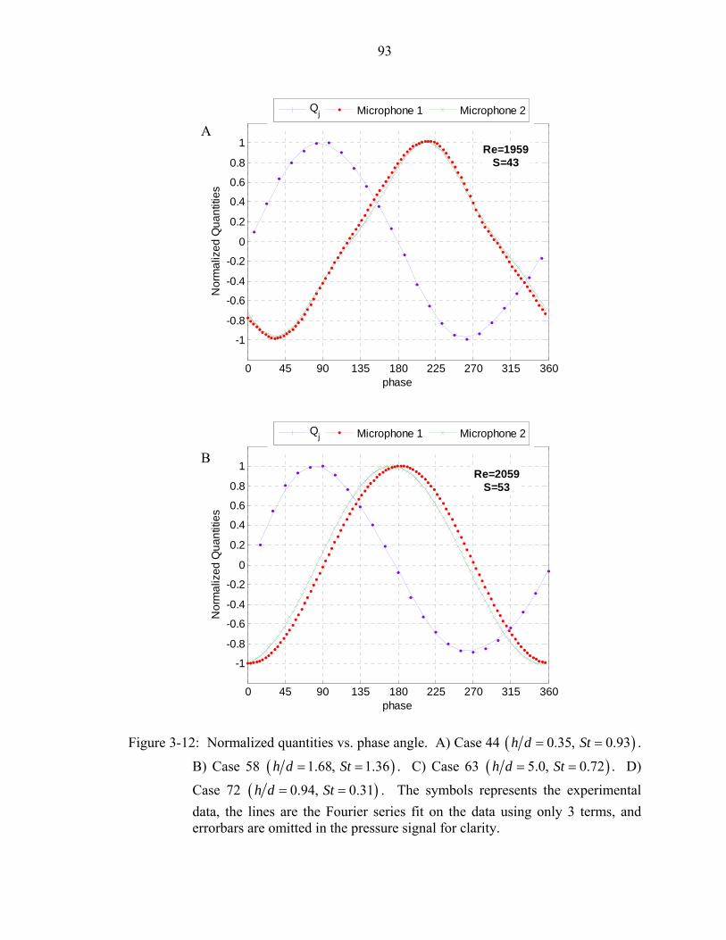
93

0 45 90 135 180 225 270 315 360

-1

-0.8

-0.6

-0.4

-0.2

0

0.2

0.4

0.6

0.8

1

phase

Nor

mal

ized

Qua

ntiti

es

Re=1959S=43

0 45 90 135 180 225 270 315 360

-1

-0.8

-0.6

-0.4

-0.2

0

0.2

0.4

0.6

0.8

1

phase

Nor

mal

ized

Qua

ntiti

es

Re=2059S=53

Figure 3-12: Normalized quantities vs. phase angle. A) Case 44 ( )0.35, 0.93h d St= = .

B) Case 58 ( )1.68, 1.36h d St= = . C) Case 63 ( )5.0, 0.72h d St= = . D)

Case 72 ( )0.94, 0.31h d St= = . The symbols represents the experimental data, the lines are the Fourier series fit on the data using only 3 terms, and errorbars are omitted in the pressure signal for clarity.

B

A

Qj Microphone 1 Microphone 2


94

0 45 90 135 180 225 270 315 360

-1

-0.8

-0.6

-0.4

-0.2

0

0.2

0.4

0.6

0.8

1

phase

Nor

mal

ized

Qua

ntiti

es

Re=286S=14

0 45 90 135 180 225 270 315 360

-1

-0.8

-0.6

-0.4

-0.2

0

0.2

0.4

0.6

0.8

1

phase

Nor

mal

ized

Qua

ntiti

es

Re=179 S=4

Figure 3-12: Continued.

To determine the number of relevant harmonics that capture the principal features

of the signal, a vector averaged power spectrum analysis is performed for each individual

case, as shown for four cases in Figure 3-13, and Table G-1 in Appendix G summarizes

the percentage power contained in the fundamental and each harmonic along with the

corresponding square of the residual norm. Clearly, although more than 90% of the total

C

D



95

power in the signal is present at the fundamental, the contribution from subsequent

harmonics may not be negligible, especially from the 2nd harmonic (at 03 f ). There exist

several criteria to determine the degree of confidence in the relevant harmonics to keep in

the Fourier series reconstruction. Here, we use the residual of the least squares fit, where

the signal is decomposed into k components until the least square estimation of the

(k+1)th harmonic only fits noise, hence reaching a negligible residual value. This can be

seen from Figure 3-13. Once the number of significant harmonics retained in the signal

has been validated for each case, the Fourier series fit to the waveforms for the volume

flow rate and the two pressure signals are plotted on top of the data points as a function of

phase, as shown in Figure 3-12 for selected cases. In these cases, only the first 3

harmonics in the signals are kept.

0 1000 2000 3000 4000 5000

100

105

[Pa rm

s2

]

Power spectrum - Case 44

Microphone 1Microphone 2

010

-15

10-10

[ µm

rms

2]

Diaphragm

Figure 3-13: Power spectrdisplacement. A

( 1.68, 1.h d St= =

( 0.94, 0h d St= =

0 500f Hz=

A

1000 2000 3000 4000 5000Frequency (Hz)

um of the two pressure recorded and the diaphragm ) Case 44 ( )0.35, 0.93h d St= = . B) Case 58

)36 . C) Case 63 ( )5.0, 0.72h d St= = . D) Case 72

).31 . The symbols are exactly at the harmonics locations.

96

0 1000 2000 3000 4000 5000 6000 7000

100

105

[Pa rm

s2

]



0 100

10-10

[ µm

rms

2]

Diaphragm

0 1

100

[Pa rm

s2

]

010

-15

10-10

[ µm

rms

2]


0 780f Hz=

B

C

0 2000 3000 4000 5000 6000 7000Frequency (Hz)

000 2000 3000 4000 5000



Diaphragm0 500f Hz=

1000 2000 3000 4000 5000Frequency (Hz)

97

0 50 100 150 200 250 300 350

100

[Pa rm

s2

]



0 50

10-15

[ µm

rms

2]

Diaphragm


In addition to the above

ZNMF actuator device unde

visualization of the flow beh

ascertain whether a jet is form

region it can fall within.

Lasersource

Light sheoptics

Figure 3-14: Schematic of the

0 39f Hz=

D

100 150 200 250 300 350Frequency (Hz)

Flow Visualization

experimental setup that provides quantitative results on the

r a wide range of operating conditions, a qualitative

avior emanating from the orifice is performed, mainly to

ed or not, and if indeed a jet is formed, under which flow

Glasstank

et ZNMFactuator

Seededflow field

Lightsheet

flow visualization setup.

98

Figure 3-14 shows a schematic of the flow visualization setup, where a continuous-

watt argon-ion laser is used in conjunction with optical lenses to form a thin light sheet

centered on the orifice axis, and atomized haze fluid is introduced into the tank to seed

the flow. The topology of the orifice flow behavior is simply noted and Table 2-3 in

Chapter 2 lists the results for most of the cases. The nomenclature presented in this

dissertation is crude and far from exhaustive. The reader is referred to the detailed work

preformed by Holman (2005) for a complete qualitative and quantitative study on the

different topological regimes of ZNMF actuators exhausting into a quiescent medium.

The topological regimes identified through this test matrix only include the no flow

regime or a distinct flow pattern present at the orifice exit. In Table 2-3, it is referred to

as follows:

• X: no jet formed • J: jet formed

To conclude this chapter, an extensive experimental investigation has been

described, the results of which are used throughout this dissertation. In particular,

Chapter 4 focuses on orifice flow physics, hence presenting the results of the LDV

measurements and the flow visualization. The cavity pressure and diaphragm deflection

measurements are presented in Chapter 5 where the cavity behavior is thoroughly

investigated. Finally, Chapter 6 leverages all the information gathered and uses all these

results for the development of a refined reduced-order model.

99

CHAPTER 4

RESULTS: ORIFICE FLOW PHYSICS

This chapter presents the results of the experimental and numerical investigation

described in Chapter 3 and Appendix F, respectively. It focuses on the rich and complex

flow physics of a ZNMF actuator exhausting into a quiescent medium. The local flow

field at the orifice exit is first examined via the numerical simulations that provide useful

information on the flow pattern inside the actuator, followed by the results of the

experimentally acquired velocity profiles. Some results on the jet formation are

presented next. A detailed investigation is then performed on the influence of the

governing parameters on the orifice flow field and more generally on the actuator

performance. Finally, the diverse mechanisms that can generate non-negligible

nonlinearities in the actuator behavior are reviewed and the related limitations addressed.

Ultimately, this investigation on the orifice flow behavior will help in developing

physics-based reduced-order models of ZNMF actuators exhausting into quiescent air for

both modeling and design purposes, as detailed in Chapter 6.

The test matrix tabulated in Table 2-3 is designed to cover a significant parameter

space, in terms of nondimensional parameters, where a total of 8 numerical simulations

and 62 different experimental cases are considered. The dimensional parameters varied

in this study are the orifice diameter d and height h , the actuation frequency ω , and the

input voltage amplitude (i.e., driver amplitude). Hence, in terms of dimensionless

parameters, this corresponds to varying the orifice aspect ratio h d , the jet Reynolds

100

number Re jV d ν= , the Stokes number 2S dω ν= , the dimensionless volume

displaced by the driver 3d∆∀ , the actuation-to-Helmholtz frequency ratio Hω ω , the

actuation-to-diaphragm frequency ratio dω ω , and the dimensionless wavenumber kd .

Recall that the Reynolds, Stokes, and Strouhal numbers are related via 2 ReSt S= so

that knowledge of any two dictates the remaining quantity. The available numerical

simulations are from the George Washington University (lead by Prof. Mittal) in a

collaborative joint effort between our two groups. The methodology of the 2D numerical

simulations is provided in Appendix F. Next, the experimental setup is presented in

detail in Chapter 3, and this investigation provides information on the velocity profile

across the orifice – hence jet volume flow rate, cavity pressure oscillations, and driver

volume flow rate as a function of phase angle and in terms of the above dimensionless

parameters.

Local Flow Field

Velocity Profile through the Orifice: Numerical Results

The major limitation in the experimental setup is that it is spatially limited, in the

sense that data cannot be acquired inside the orifice. Therefore, the role of numerical

simulations that can provide information anywhere inside the computed domain is

relevant in this study. The direct numerical simulations described in detail in Appendix F

are used to understand the flow behavior inside the orifice, particularly to examine the

evolution of the velocity profile inside the slot. The test cases of interest correspond to

Case 1, 2 & 3 in Table 2-3. They have the same Reynolds number Re = 262, but have

different Stokes number (S = 25 or S = 10) and orifice aspect ratio h/d (1, 2, and 0.68, for

101

Cases 1, 2, and 3, respectively). Note also that they share a straight rectangular slot for

the orifice and that the simulations are two-dimensional.

d

h

y

x

y/h = -1

y/h = -0.5y/h = -0.75

y/h = -0.25y/h = 0

B) Case 2

D

L0/h=1.32 L0/h=0.66

L0/h=12C) Case 3

Figure 4-1: Numerical results of the orifice flow pattern showing axial and longitudinal velocities, azimuthal vorticity contours, and instantaneous streamlines at the time of maximum expulsion. A) Case 1 (h/d = 1, St = 2.38, S = 25). B) Case 2 (h/d = 2, St = 2.38, S = 25). C) Case 3 (h/d = 0.68, St = 0.38, S = 10). D) Actuator schematic with coordinate definition.

A) Case 1

102

Figure 4-1 shows the flow pattern inside the orifice for A) Case 1, B) Case 2 and C)

Case 3. The azimuthal vorticity contours are plotted along with the axial and longitudinal

velocities and some instantaneous streamlines, during the time of maximum expulsion.

Also, Figure 4-1D shows a schematic of the actuator configuration and provides the

coordinate definition and labels used. Notice the recirculation zones inside the orifice for

the cases of low stroke length L0 (Case 1 and Case 2). Clearly, the orifice flow undergoes

significant changes as a function of the geometry and actuation conditions. Therefore,

the vertical velocity profile is probed at five different locations along the orifice height

from y/h = 0 to y/h = -1 and at different phases during one cycle, as schematized in Figure

4-1D.

Figure 4-2, Figure 4-3, and Figure 4-4 show the computed vertical velocity profiles

at various locations in the orifice and corresponding at four different times during the

cycle, for Case 1, Case 2, and Case 3, respectively. Also for clarification, the azimuthal

vorticity contours are shown in each figure. First of all, it can be seen that Case 1 and

Case 2 are qualitatively similar, although the three cases show that the velocity profile

undergoes significant development along the orifice length. In particular, Figure 4-2 and

Figure 4-3 show a strong phase dependence in the velocity profile inside the orifice,

which is not the case for Case 3. Similarly, the Stokes number dependency in the shape

of the velocity profile is clearly denoted. In particular, the velocity profiles at the exit

(y/h = 0) during the time of maximum expulsion are nearly identical for Case 1 and Case

2 that have the same Stokes number, as shown in Figure 4-2B and Figure 4-3B,

respectively.

103

φC

95φ = °

Figure 4-2: =(vc

2φ = ° A B

269φ = ° 177= ° D

Velocity profile at different locations inside the orifice for Case 1 (h/d = 1, St 2.38, S = 25). A) Beginning of expulsion (2o). B) Maximum expulsion 95o). C) Beginning of ingestion (177o). D) Maximum ingestion (269o). The ertical velocity is normalized by jV . Also shown are the azimuthal vorticity ontours for each phase.

104

For the low stroke length – or high Strouhal number - cases at the maximum

expulsion time (Cases 1 and 2 in Figure 4-2B and Figure 4-3B, respectively), the

variation in the boundary layer thickness at the walls (from thin to thick as the fluid

moves toward the orifice exit), along with the variation of the core region is indicative of

the flow acceleration inside the orifice. This tangential acceleration of fluid at the

boundary wall generates vorticity (Morton 1984). Also, notice the smoother profiles near

the walls along the orifice length for the time of beginning of the expulsion stroke (Figure

4-2A and Figure 4-3A) and beginning of the ingestion stroke (Figure 4-2C and Figure

4-3C), compared when the cycle reaches its maximum expulsion and ingestion (Figure

4-2B and Figure 4-2D, and Figure 4-3B and Figure 4-3D). At the time of maximum

expulsion velocity ( )90φ = ° , for these two cases of high Strouhal number where no jet is

formed, the velocity profiles are influenced by the vorticity that is not expelled at the exit

(or inlet during maximum ingestion) and is trapped inside the orifice, leading to

secondary vortices.

In the case of a larger stroke length (L0/h = 12), as seen in Figure 4-4, the flow is

always reversed near the walls. Interestingly, in Case 3 the flow is “similar” along the

orifice height – roughly independent of y, but is still dependant of the phase angle, hence

of time. Notice that in this case where the stroke length is much larger than the orifice

height, the flow is dominated by entrance and exit losses, where viscous effects are

confined at the walls and the core region is moving in phase at each y location along the

orifice. In this case, the flow never reaches a fully developed stage, as shown in Figure

4-4C.

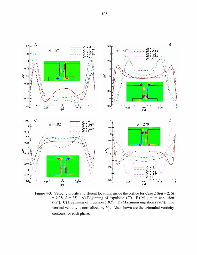
105

A B

C D

2φ = ° 92φ = °

182φ = ° 270φ = °

Figure 4-3: Velocity profile at different locations inside the orifice for Case 2 (h/d = 2, St = 2.38, S = 25). A) Beginning of expulsion (2o). B) Maximum expulsion (92o). C) Beginning of ingestion (182o). D) Maximum ingestion (270o). The vertical velocity is normalized by jV . Also shown are the azimuthal vorticity contours for each phase.

106

A

0φ = °

D

φ =

C

180φ = °

Figure 4-4: Velocity profile at different locations inside0.68, St = 0.38, S = 10). A) Beginning of expulsion (90o). C) Beginning of ingestion (1(270o). The vertical velocity is normalized azimuthal vorticity contours for each phase.

90φ = °

B

270°

the orifice for Case 3 (h/d = expulsion (0o). B) Maximum 80o). D) Maximum ingestion by jV . Also shown are the

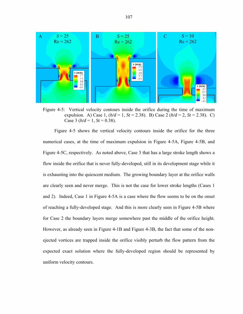
107

S = 25

Re = 262 A B C

Figure 4-5: Vertical velocity contours inside the orifice during the time of maximum

expulsion. A) Case 1, (h/d = 1, St = 2.38). B) Case 2 (h/d = 2, St = 2.38). C) Case 3 (h/d = 1, St = 0.38).

Figure 4-5 shows the vertical velocity contours inside the orifice for the three

numerical cases, at the time of maximum expulsion in Figure 4-5A, Figure 4-5B, and

Figure 4-5C, respectively. As noted above, Case 3 that has a large stroke length shows a

flow inside the orifice that is never fully-developed, still in its development stage while it

is exhausting into the quiescent medium. The growing boundary layer at the orifice walls

are clearly seen and never merge. This is not the case for lower stroke lengths (Cases 1

and 2). Indeed, Case 1 in Figure 4-5A is a case where the flow seems to be on the onset

of reaching a fully-developed stage. And this is more clearly seen in Figure 4-5B where

for Case 2 the boundary layers merge somewhere past the middle of the orifice height.

However, as already seen in Figure 4-1B and Figure 4-3B, the fact that some of the non-

ejected vortices are trapped inside the orifice visibly perturb the flow pattern from the

expected exact solution where the fully-developed region should be represented by

uniform velocity contours.

S = 10 Re = 262

S = 25 Re = 262

108

On the other hand, one can interpret the flow pattern shown in Figure 4-5 with a

different point of view. For instance, a vena contracta can be seen in Case 1 and Case 2

(Figure 4-5A and Figure 4-5B, respectively), but a core flow moving in phase in Case 3

(Figure 4-5C). None of these three cases are “fully-developed” in the strict sense

(velocity profile invariant of position y). Clearly, Cases 1 and 2 are affected by the

trapped z-vorticity that is generated at the wall and at the orifice leaps; and in the absence

of this z-vorticity, the flow would appear to be fully-developed. Contrarily, for Case 3

(Figure 4-5C) the vena contracta extends the full height of the orifice and the flow never

reaches a fully-developed stage.

On the vorticity dynamics inside the orifice, the generation of the azimuthal or z-

vorticity comes from the pressure gradient present at the sharp edges of the orifice exit

(and inlet), and of the fluid tangential acceleration at the wall boundary inside the orifice.

This generation process is instantaneous and inviscid (Morton 1984). However, the

“decay” or “destruction” of vorticity only results from the cross-diffusion of the two

vorticity fluxes that are of opposite sense and that occurs at the center line. Here, the

diffusion time scale for vorticity to diffuse across the slot is

2vist d ν∼ , (4-1)

and the convective time scale for a fluid particle to travel the orifice height is given by

conv jt h V∼ . (4-2)

Therefore, the ratio of the time scales,

2

Rejvis

conv

Vt d dt h hν

∼ ∼ , (4-3)

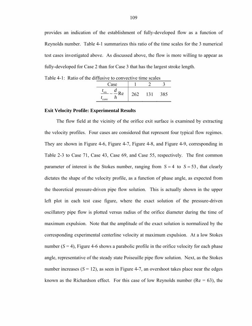
109

provides an indication of the establishment of fully-developed flow as a function of

Reynolds number. Table 4-1 summarizes this ratio of the time scales for the 3 numerical

test cases investigated above. As discussed above, the flow is more willing to appear as

fully-developed for Case 2 than for Case 3 that has the largest stroke length.

Table 4-1: Ratio of the diffusive to convective time scales Case 1 2 3

Revis

conv

t dt h

∼ 262 131 385

Exit Velocity Profile: Experimental Results

The flow field at the vicinity of the orifice exit surface is examined by extracting

the velocity profiles. Four cases are considered that represent four typical flow regimes.

They are shown in Figure 4-6, Figure 4-7, Figure 4-8, and Figure 4-9, corresponding in

Table 2-3 to Case 71, Case 43, Case 69, and Case 55, respectively. The first common

parameter of interest is the Stokes number, ranging from 4S = to 53S = , that clearly

dictates the shape of the velocity profile, as a function of phase angle, as expected from

the theoretical pressure-driven pipe flow solution. This is actually shown in the upper

left plot in each test case figure, where the exact solution of the pressure-driven

oscillatory pipe flow is plotted versus radius of the orifice diameter during the time of

maximum expulsion. Note that the amplitude of the exact solution is normalized by the

corresponding experimental centerline velocity at maximum expulsion. At a low Stokes

number (S = 4), Figure 4-6 shows a parabolic profile in the orifice velocity for each phase

angle, representative of the steady state Poiseuille pipe flow solution. Next, as the Stokes

number increases (S = 12), as seen in Figure 4-7, an overshoot takes place near the edges

known as the Richardson effect. For this case of low Reynolds number (Re = 63), the

110

Figure 4-6: Experimental vertical velocity profiles across the orifice for a ZNMF

actuator in quiescent medium at different instant in time for Case 71: Re 112= , 0.94h d = , 0.1y d = . The solid line in the upper left plot is the exact solution of oscillatory pipe flow, normalized by the experimental centerline velocity, at maximum expulsion. The zero phase corresponds to the start of the expulsion cycle.

velocity profile seems to be slightly different from expulsion to ingestion times in the

cycle. As the Stokes number increases further, as in Figure 4-8 where S = 17, the

overshoot is less pronounced, but the Reynolds number is much higher (Re = 1361) and

now the ingestion and expulsion profiles exhibit less variation in their profiles. Notice

also that in this case, the orifice aspect ratio is 5h d = and 0 0.9L h = is less than unity

so the flow is expected to reach a fully-developed state, compared with Case 43 in Figure

-0.6 -0.4 -0.2 0 0.2 0.4 0.6-1.8

-1.6

-1.4

-1.2

-1

-0.8

-0.6

-0.4

-0.2

0

0.2

∆φ=15°

φ

-0.6 -0.4 -0.2 0 0.2 0.4 0.6-1.8

-1.6

-1.4

-1.2

-1

-0.8

-0.6

-0.4

-0.2

0

0.2

∆φ=15°

φ

-0.6 -0.4 -0.2 0 0.2 0.4 0.60

0.5

1

1.5

2

2.5

3

3.5

4

4.5

φ

∆φ=15°

-0.6 -0.4 -0.2 0 0.2 0.4 0.60

0.5

1

1.5

2

2.5

3

3.5

4

4.5

exactsolution

∆φ=15°

φ

π/2

π

3π/2

0

π/4π/2

π

3π/2

0

3π/4

π/2

π

3π/2

05π/4

π/2

π

3π/2

0

7π/4

S=4 St=0.14

vertical velocity (m/s) vertical velocity (m/s)

r/d r/d

111

4-7 where for a similar Stokes number (S = 12), the orifice aspect ratio is less than unity

and the stroke length is greater than the orifice height ( )0 1.3L h = , meaning that the flow

may not reach a fully-developed state and is dominated by entrance and exit region

effects. Finally, the case of highest Stokes number (S = 53) shows a nearly slug velocity

profile, as seen in Figure 4-9. Note that in this case, no jet is formed at the orifice lip.


actuator in quiescent medium at different instant in time for Case 43: Re 63= , 0.35h d = , 0.03y d = . The solid line in the upper left plot is the exact

solution of oscillatory pipe flow, normalized by the experimental centerline velocity, at maximum expulsion. The zero phase corresponds to the start of the expulsion cycle.

-0.6 -0.4 -0.2 0 0.2 0.4 0.6

-0.5

-0.4

-0.3

-0.2

-0.1

0

0.1∆φ=15°

φ

-0.6 -0.4 -0.2 0 0.2 0.4 0.6

-0.5

-0.4

-0.3

-0.2

-0.1

0

0.1∆φ=15°

φ

-0.6 -0.4 -0.2 0 0.2 0.4 0.6-0.1

0

0.1

0.2

0.3

0.4

0.5

0.6

0.7

0.8exact

solution

∆φ=15°

φ

-0.6 -0.4 -0.2 0 0.2 0.4 0.6-0.1

0

0.1

0.2

0.3

0.4

0.5

0.6

0.7

0.8

∆φ=15°

φ

π/2

π

3π/2

0

7π/4

π/2

π

3π/2

05π/4

π/2

π

3π/2

0

3π/4π/2

π

3π/2

0

π/4

S=12 St=2.23

r/d r/d

vertical velocity (m/s) vertical velocity (m/s)

112

Another interesting result comes from a comparison of these experimental velocity

profiles with the theoretical ones, as shown in each figure in the upper left plot. Notice

that the overall profile, particularly the overshoot near the wall if present, is well

represented. However, because of the finite distance off the orifice surface at which the

LDV data have been acquired (y/d = 0.1, 0.03, 0.1, and 0.03 for Case 71, 43, 69, and 55,

respectively), the profiles cannot exactly match at the orifice edge. An additional reason

for the difference noticed between the exact solution and the experimental results is that

the flow may not be fully-developed by the time it reaches the orifice exit. Recall that the

theoretical solution assumes a fully-developed flow inside the orifice, meaning the

boundary layer forming at the orifice entrance has finally merged. If not, the flow is still

evolving along the length of the orifice. Hence, it would be like having an effective

diameter -less than the actual one- for which the exact solution should be valid (a change

in the diameter d will change the Stokes number S and the shape of the velocity profile).

This remark is important for modeling purposes.

For the four cases represented here, and actually for all the experimental test cases

considered in this study, notice the large velocity gradients near the edge of the orifice

that the LDV experimental setup is able to accurately capture. Especially for the large

Reynolds number case (Case 69) in Figure 4-8, where the vertical velocity jumps from

about zero to 40 m/s over a length scale of 0.3 mm. Similarly, it can be seen from these

plots that, although the edges of the orifice are at 0.5r d = ± , the velocity tends to a zero

value beyond the orifice lip. This is due to the fact that the LDV data have been acquired

at a finite distance y d above the orifice surface, and that fluid entrainment is significant

near the edge of the axisymmetric orifice. Indeed, although not shown here for these

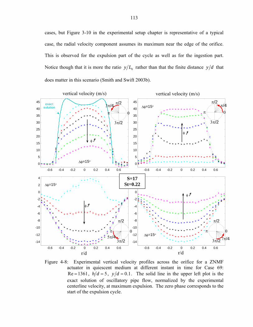
113

cases, but Figure 3-10 in the experimental setup chapter is representative of a typical

case, the radial velocity component assumes its maximum near the edge of the orifice.

This is observed for the expulsion part of the cycle as well as for the ingestion part.

Notice though that it is more the ratio 0y L rather than that the finite distance y d that

does matter in this scenario (Smith and Swift 2003b).


actuator in quiescent medium at different instant in time for Case 69: Re 1361= , 5h d = , 0.1y d = . The solid line in the upper left plot is the exact solution of oscillatory pipe flow, normalized by the experimental centerline velocity, at maximum expulsion. The zero phase corresponds to the start of the expulsion cycle.

-0.6 -0.4 -0.2 0 0.2 0.4 0.6

-14

-12

-10

-8

-6

-4

-2

0

2

4

φ

∆φ=15°

-0.6 -0.4 -0.2 0 0.2 0.4 0.6

-14

-12

-10

-8

-6

-4

-2

0

2

4

φ

∆φ=15°

-0.6 -0.4 -0.2 0 0.2 0.4 0.6

0

5

10

15

20

25

30

35

40

45

φ

exactsolution

∆φ=15°

-0.6 -0.4 -0.2 0 0.2 0.4 0.6

0

5

10

15

20

25

30

35

40

45

φ

∆φ=15°

S=17 St=0.22

r/d

vertical velocity (m/s) π/2

π

3π/2

0

π/4π/2

π

3π/2

0

3π/4

π/2

π

3π/2

05π/4

π/2

π

3π/2

0

7π/4

vertical velocity (m/s)

r/d

114


actuator in quiescent medium at different instant in time for Case 55: Re 125= , 1.68h d = , 0.03y d = . The solid line in the upper left plot is the exact solution of oscillatory pipe flow, normalized by the experimental centerline velocity, at maximum expulsion. The zero phase corresponds to the start of the expulsion cycle.

Next, in terms of phase angle during an entire cycle, as seen in all these plots, the

velocity profiles are clearly phase dependent. Notice also that the profiles are not

symmetric from the expulsion to the ingestion periods, especially in magnitude, the

ingestion part having usually a broader velocity profile with decreased amplitude.

Clearly, during the expulsion phase the flow is ejected into quiescent medium similar to a

-0.6 -0.4 -0.2 0 0.2 0.4 0.6

-0.8

-0.7

-0.6

-0.5

-0.4

-0.3

-0.2

-0.1

0

0.1

0.2

∆φ=15°

φ

-0.6 -0.4 -0.2 0 0.2 0.4 0.6

-0.8

-0.7

-0.6

-0.5

-0.4

-0.3

-0.2

-0.1

0

0.1

0.2

∆φ=15°

φ

-0.6 -0.4 -0.2 0 0.2 0.4 0.6-0.1

0

0.1

0.2

0.3

0.4

0.5

0.6

0.7

0.8

0.9exact

solution

φ

∆φ=15°

-0.6 -0.4 -0.2 0 0.2 0.4 0.6-0.1

0

0.1

0.2

0.3

0.4

0.5

0.6

0.7

0.8

0.9

φ

∆φ=15°

S=53 St=22.3


r/d r/d


π/2

π

3π/2

0

7π/4

π/2

π

3π/2

05π/4

π/2

π

3π/2

0

π/4

π/2

π

3π/2

0

3π/4

115

steady jet, whereas during the ingestion phase, the flow is similar to that in the entrance

region of a steady pipe flow. This observation corroborates our global approach outlined

in Chapter 2 in making a clear distinction between the expulsion and the ingestion portion

of the cycle. Also, it is worthwhile to note that all the test cases considered in this

dissertation are close to zero-net mass flux. For instance, for the four experimental cases

discussed above, the ratio between totQ , the total volume flow rate during one cycle, and

jQ , the volume flow rate during the expulsion part of the cycle, is equal to 0.17, 0.01,

0.39, and 0.09, for Cases 71, 43, 69, and 55, respectively. The total volume flow rate

being at least an order of magnitude lower than that during the expulsion part, the zero-

net mass flux condition is indeed verified.

Finally, another interesting observation is found in the relationship between the

centerline velocity ( )CLV t at the exit and the corresponding mean – or spatially averaged

– velocity ( ) ( )2j jV t Vπ= . This is shown in Figure 4-10A and Figure 4-10B where the

ratio of the two time-averaged velocities is plotted versus Stokes number and Reynolds

number, respectively. For instance, it is expected that 2 2CL j jV V V= = for the steady

Poseuille flow, which is seen in Figure 4-10A, while for high Stokes number where the

velocity profile is expected to be slug-like, it should asymptotes to unity. Recall the

analytical solution for an oscillatory pipe flow shown in Figure 2-5 and plotted again in

Figure 4-10A. However, there is no such well-defined behavior for all the cases studied

here that will dictate a scaling law for this velocity ratio.

116

1 10 1000.5

0.6

0.7

0.8

0.9

1

1.1

1.2

1.3

1.4

S

Vj /

Vj,C

L

0<Re<100100<Re<200200<Re<500500<Re<900900<Re<14002000<Re<3000

solution forfully-developed

pipe flow

0 500 1000 1500 2000 2500 3000 35000.5

0.6

0.7

0.8

0.9

1

1.1

1.2

1.3

1.4

Re

Vj /

Vj,C

L

S=4S=12S=14S=17S=43S=53

Figure 4-10: Experimental results of the ratio between the time- and spatial-averaged

velocity jV and time-averaged centerline velocity ,j CLV . A) Versus Stokes number S. B) Versus Reynolds number Re.

Jet Formation

Next, the question whether a jet is formed or not at the orifice exit is investigated,

since it has been shown in the previous sections that this criterion may influence on the

orifice flow dynamics. Past simulations and experiments have shown that the vorticity

A

B

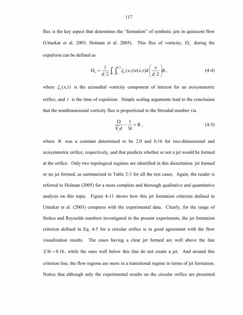
117

flux is the key aspect that determines the “formation” of synthetic jets in quiescent flow

(Utturkar et al. 2003, Holman et al. 2005). This flux of vorticity, vΩ during the

expulsion can be defined as

2

0 0

1 ( , ) ( , )2 2

d

v zxx t v x t d dt

d dτ

ξ⎛ ⎞

Ω = ⎜ ⎟⎝ ⎠

∫ ∫ , (4-4)

where ( , )z x tξ is the azimuthal vorticity component of interest for an axisymmetric

orifice, and τ is the time of expulsion. Simple scaling arguments lead to the conclusion

that the nondimensional vorticity flux is proportional to the Strouhal number via

1

j

KStV d

Ω>∼ , (4-5)

where K was a constant determined to be 2.0 and 0.16 for two-dimensional and

axisymmetric orifice, respectively, and that predicts whether or not a jet would be formed

at the orifice. Only two topological regimes are identified in this dissertation: jet formed

or no jet formed, as summarized in Table 2-3 for all the test cases. Again, the reader is

referred to Holman (2005) for a more complete and thorough qualitative and quantitative

analysis on this topic. Figure 4-11 shows how this jet formation criterion defined in

Utturkar et al. (2003) compares with the experimental data. Clearly, for the range of

Stokes and Reynolds numbers investigated in the present experiments, the jet formation

criterion defined in Eq. 4-5 for a circular orifice is in good agreement with the flow

visualization results. The cases having a clear jet formed are well above the line

1 0.16St = , while the ones well below this line do not create a jet. And around this

criterion line, the flow regions are more in a transitional regime in terms of jet formation.

Notice that although only the experimental results on the circular orifice are presented

118

here, the numerical simulations featuring a rectangular slot and shown in Table 2-3 do

satisfy the jet formation criterion as well. Consequently, this investigation on the jet

formation criterion, validated through the flow visualization results, gives confidence in

using this criterion for the description of the orifice flow behavior.

101 102 103 104100

101

102

103

104

S2

Re

jet

no jet

1/St=0.16

Figure 4-11: Experimental results on the jet formation criterion.

Influence of Governing Parameters

In this section, the governing parameters extracted from the dimensional analysis

and described in Chapter 2 are applied in this experimental investigation in order to

confirm their validity and also investigate their respective influence on the ZNMF

actuator behavior. The functional form (Eq. 2-15) is reproduced for illustration,

3, , , , , ,Re

j d

H d

Q Qh wSt fn kd Sd d d

ω ωω ω

⎫⎪ ⎛ ⎞∆∀⎪ =⎬ ⎜ ⎟

⎝ ⎠⎪⎪⎭

. (4-6)

Note that the role of the Helmholtz frequency and of the cavity size and driver

characteristics ( )3; ; ;H dd kdω ω ω ω∆∀ is not addressed in this section, the next

119

chapter being entirely dedicated to them. Since the experimental test only uses

axisymmetric orifices, the functional form for fixed driver/cavity parameters can be

recast as

,ReSt hfn S

d⎫ ⎛ ⎞=⎬ ⎜ ⎟

⎝ ⎠⎭. (4-7)

So any two parameters between the Strouhal number, Reynolds number and Stokes

number, plus the orifice aspect ratio should suffice in describing the ZNMF actuator flow

characteristics. For completeness, as mentioned at the end of Chapter 2 in the description

of the different regimes of the orifice flow, recall the dimensionless stroke length that is

simply related to the above parameters by

02

Re 1L d dh h S h St

π π⎛ ⎞ ⎛ ⎞= =⎜ ⎟ ⎜ ⎟⎝ ⎠ ⎝ ⎠

, (4-8)

where the constant π ωτ= comes from the assumption of a sinusoidal jet velocity.

Before presenting some results on the experimental data, a remark should be made

concerning their interpretation. As explained previously, the cavity pressure fluctuations

are used in lieu of the pressure drop across the orifice since experimentally, it is rather

difficult to acquire the dynamic pressure drop across the orifice for such small devices.

However, the acquired cavity pressure may deviate from the actual pressure drop through

the orifice. This will be discussed further in Chapter 5.

Empirical Nonlinear Threshold

First of all, the “current” approach to characterize or “calibrate” an oscillatory

fluidic actuator that was first indirectly addressed by Ingard and Labate (1950) and more

recently by Seifert and Pack (1999) is applied here, which uses the simple empirical

observation that the cavity pressure fluctuation p∆ is linearly proportional to the

120

centerline exit velocity fluctuation CLv at low forcing levels, and to 2CLv (i.e., nonlinear) at

sufficiently high forcing levels. Figure 4-12 shows the variation of the averaged jet

velocity jV to the cavity fluctuating pressure cP∆ for a specific Stokes number. Notice

that two scaling regions can be extracted from this plot, i.e. as the pressure amplitude

increases the jet velocity varies from a linear to a nonlinear scaling dependence.

10-1

100

101

102

103

104

10-2

10-1

100

101

102

∆Pc/ρ

Vj

S=4S=8S=17S=53

Vj2 ~ ∆Pc/ρc0

Vj ~ ∆Pc/ρ

Figure 4-12: Averaged jet velocity vs. pressure fluctuation for different Stokes number.

However, the threshold level from which the linear proportionality can be

distinguished from the nonlinear one varies as a function of the Stokes number. Clearly,

this “calibration” curve is Stokes number dependant and practically useless. This

analysis is based only on the velocity and pressure information and thus lacks crucial

nondimensional parameters to be taken into account to capture more physics. This

motivates the dimensional analysis performed in Chapter 2, and the dependency of the

actuator behavior on those parameters is investigated next.

121

Strouhal, Reynolds, and Stokes Numbers versus Pressure Loss

Consider the loss mechanisms inside the orifice, especially the minor nonlinear

losses. Nonlinear losses are known to be dependant on the flow parameters and, in the

case of steady flow, empirical laws already exist (White 1991). However, for an

oscillatory pipe or channel flow, this topic is still the focus of current research. Here, a

physics-based qualitative description on the nonlinear loss mechanism is attempted. The

nonlinear loss coefficient can be written as

20.5

cd

j

PKVρ

∆= , (4-9)

where cP∆ represents the cavity pressure fluctuations which is equivalent to the pressure

drop across the orifice for a ZNMF actuator (see Chapter 5 for more details on the

pressure equivalence), and 2

0.5 jVρ is the dynamic pressure based on the time and

spatial-averaged expulsion velocity at the orifice exit jV .

The experimentally determined loss coefficient dK is plotted versus St h d⋅ ,

which is equivalent to the ratio of the stroke length to the orifice height, is shown in

Figure 4-13A and Figure 4-13B using linear and logarithmic scales, respectively. Notice

that the 3 numerical simulation results discussed above are also included for comparison.

From the linear scale, Figure 4-13A, the pressure loss data asymptote to a constant value

of order of magnitude ( )1O as ( )0St h d h L⋅ ∝ decreases beyond a certain value. This

suggests that when the fluid particle excursion or stroke length is much larger than the

orifice height h, minor “nonlinear” losses due to entrance and exit effects dominate the

flow. However, the magnitude of these losses and the degree of nonlinear distortion is

likely to be strongly dependent on Reynolds number, in a similar manner as for the steady

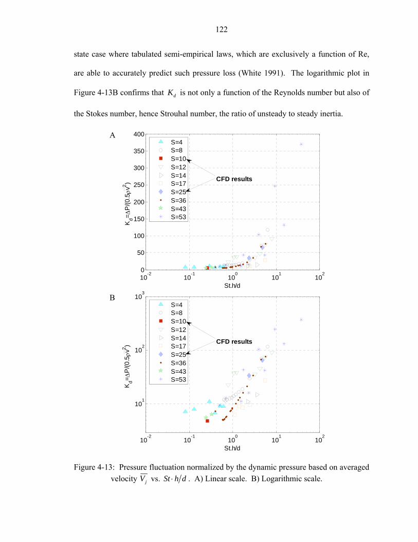
122

state case where tabulated semi-empirical laws, which are exclusively a function of Re,

are able to accurately predict such pressure loss (White 1991). The logarithmic plot in

Figure 4-13B confirms that dK is not only a function of the Reynolds number but also of

the Stokes number, hence Strouhal number, the ratio of unsteady to steady inertia.

10-2

10-1

100

101

102

0

50

100

150

200

250

300

350

400

St.h/d

Kd= ∆

P/(0

.5ρv

2 )

S=4S=8S=10S=12S=14S=17S=25S=36S=43S=53

CFD results

10-2

10-1

100

101

102

101

102

103

St.h/d

Kd= ∆

P/(0

.5ρv

2 )

S=4S=8S=10S=12S=14S=17S=25S=36S=43S=53

CFD results

Figure 4-13: Pressure fluctuation normalized by the dynamic pressure based on averaged velocity jV vs. St h d⋅ . A) Linear scale. B) Logarithmic scale.

A

B

123

10-2

10-1

100

101

102

0

50

100

150

200

250

300

350

400

St

Kd= ∆

P/(0

.5ρv

2 )

S=4S=8S=10S=12S=14S=17S=25S=36S=43S=53

CFD results

10-2

10-1

100

101

102

101

102

103

St

Kd= ∆

P/(0

.5ρv

2 )

S=4S=8S=10S=12S=14S=17S=25S=36S=43S=53

CFD results

Figure 4-14: Pressure fluctuation normalized by the dynamic pressure based on averaged

velocity jV vs. Strouhal number. A) Linear scale. B) Logarithmic scale.

Interestingly, the loss coefficient is again shown in Figure 4-14 in a linear and

logarithmic scale, but this time as a function of the Strouhal number only. Notice the

linear plot shows better collapse in the data for high Strouhal number, i.e. for unsteady

inertia greater than steady inertia, while for low Strouhal numbers, not much difference is

noticed. This suggests that their exists 2 distinct regimes in which the loss coefficient

B

A

124

dK is primarily a function of the Strouhal number for high St, while for low St, a

dimensionless stroke length may be more appropriate in describing the variations in dK .

S = 25

Re = 262 S = 25

Re = 262

A B

Figure 4-15: Vorticity contours during the maximum expulsion portion of the cycle from

numerical simulations. A) Case 1 (h/d = 1, St = 2.38). B) Case 2 (h/d = 2, St = 2.38). C) Case 3 (h/d = 1, St = 0.38).

As previously discussed in Gallas et al. (2004), the results of numerical simulations

allow detailed investigation of these issues. Again, CFD simulations have the capability

to provide information everywhere in the computed domain. Figure 4-15 shows the

variation of the spanwise vorticity for the three computational cases (Case 1, 2 and 3) at

the time of maximum expulsion. As already shown in Figure 4-11 on the jet formation

criterion, for Cases 1 and 2 no jet is formed (Figure 4-15A and Figure 4-15B), whereas

for Case 3 a clear jet is formed (Figure 4-15C). The spanwise vorticity contours show

that the vortices formed during the expulsion cycle for Case 1 and 2 are ingested back

S = 10 Re = 262

C

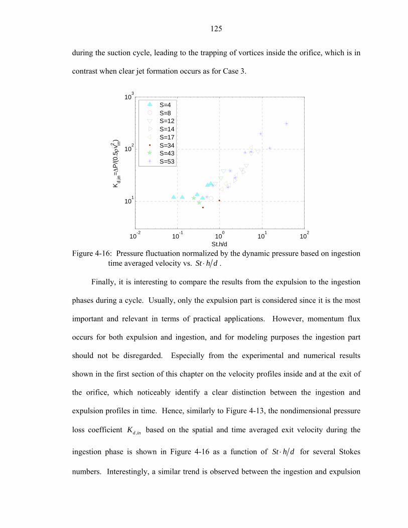
125

during the suction cycle, leading to the trapping of vortices inside the orifice, which is in

contrast when clear jet formation occurs as for Case 3.

10-2

10-1

100

101

102

101

102

103

St.h/d

Kd,

in= ∆

P/(0

.5ρv

in2)

S=4S=8S=12S=14S=17S=34S=43S=53

Figure 4-16: Pressure fluctuation normalized by the dynamic pressure based on ingestion

time averaged velocity vs. St h d⋅ .

Finally, it is interesting to compare the results from the expulsion to the ingestion

phases during a cycle. Usually, only the expulsion part is considered since it is the most

important and relevant in terms of practical applications. However, momentum flux

occurs for both expulsion and ingestion, and for modeling purposes the ingestion part

should not be disregarded. Especially from the experimental and numerical results

shown in the first section of this chapter on the velocity profiles inside and at the exit of

the orifice, which noticeably identify a clear distinction between the ingestion and

expulsion profiles in time. Hence, similarly to Figure 4-13, the nondimensional pressure

loss coefficient ,d inK based on the spatial and time averaged exit velocity during the

ingestion phase is shown in Figure 4-16 as a function of St h d⋅ for several Stokes

numbers. Interestingly, a similar trend is observed between the ingestion and expulsion

126

time of the cycle. This observation is further validated via the analysis of the numerical

data, where similarly to the data presented in Figure 4-15, the spanwise vorticity contours

occurring during the maximum ingestion are shown for Cases 1, 2 and 3 in Figure 4-17.

S = 25

Re = 262 S = 25

Re = 262

S = 10 Re = 262

A B

C

Figure 4-17: Vorticity contours during the maximum ingestion portion of the cycle from

numerical simulations. A) Case 1 (h/d = 1, St = 2.38). B) Case 2 (h/d = 2, St = 2.38). C) Case 3 (h/d = 1, St = 0.38).

This is an important result that will be used later on when developing the reduced-

order models of ZNMF actuators in Chapter 6. Indeed, the analysis of the oscillatory

flow through a symmetric orifice (i.e., same geometry on both ends) can be simplified as

follows: whatever is true during the expulsion stroke will be valid for the ingestion

stroke as well. The experimental setup only permits measurement of the exhaust flow

during expulsion and inlet flow during ingestion. During the expulsion phase, the flow at

the orifice exit sees a baffled open medium where the flow exhausts, while during the

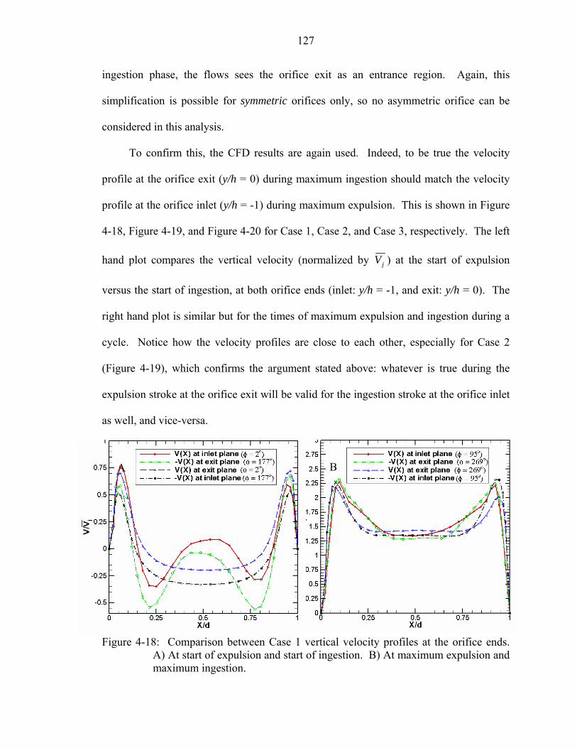
127

ingestion phase, the flows sees the orifice exit as an entrance region. Again, this

simplification is possible for symmetric orifices only, so no asymmetric orifice can be

considered in this analysis.

To confirm this, the CFD results are again used. Indeed, to be true the velocity

profile at the orifice exit (y/h = 0) during maximum ingestion should match the velocity

profile at the orifice inlet (y/h = -1) during maximum expulsion. This is shown in Figure

4-18, Figure 4-19, and Figure 4-20 for Case 1, Case 2, and Case 3, respectively. The left

hand plot compares the vertical velocity (normalized by jV ) at the start of expulsion

versus the start of ingestion, at both orifice ends (inlet: y/h = -1, and exit: y/h = 0). The

right hand plot is similar but for the times of maximum expulsion and ingestion during a

cycle. Notice how the velocity profiles are close to each other, especially for Case 2

(Figure 4-19), which confirms the argument stated above: whatever is true during the

expulsion stroke at the orifice exit will be valid for the ingestion stroke at the orifice inlet

as well, and vice-versa.

Figure 4-18: Comparison between Case 1 vertical velocity profiles at the orifice ends.

A) At start of expulsion and start of ingestion. B) At maximum expulsion and maximum ingestion.

B A

128





Nonlinear Mechanisms in a ZNMF Actuator

In view of the experimental results, the effect of the different nonlinear

mechanisms present in the system may be a critical issue that needs to be addressed if one

B A

B A

129

wants to gain confidence in the interpretation and the use of the experimental data. If one

“takes a ZNMF actuator apart,” it is basically comprised of the driver (a piezoelectric

diaphragm in the case of the current experimental tests), the cavity, and the orifice.

Hence, by considering the pressure fluctuation signal as the output signal of interest,

nonlinearities in this signal can arise due to:

1. orifice nonlinearities 2. cavity nonlinearities 3. driver nonlinearities

First, the oscillatory nature of the flow through the orifice can generate

nonlinearities in the pressure signal due to the entrance and exit regions. These

nonlinearities are the focus of this dissertation, the goal being to isolate them in order to

develop a suitable reduced-order model that accounts for these types of nonlinearities in

the pressure signal. Before proceeding down this path, we first need to understand how

nonlinearities due to the cavity pressure fluctuations and the driver scale with operating

conditions.

Starting with the cavity pressure fluctuations, nonlinearities in the signal can arise

due to deviations of the sound speed from the isentropic small-signal sound speed

(Blackstock 2000, pp. 34-35). The general isentropic equation of state

( ) 0p p p pρ ′= = + can be expressed in terms of a Taylor series expansion, such that

( ) ( )( )

20

2

0

0 0 0

1 1 21

2! 3!c

ppγ γ γγ ρ ρρ

ρ ρ ρ

⎡ ⎤− − − ⎛ ⎞′ ′′ ′ ⎢ ⎥= + + +⎜ ⎟

⎢ ⎥⎝ ⎠⎣ ⎦… , (4-10)

where γ is the ratio of specific heats, and the superscript / denotes fluctuating quantities

and the subscript 0 denotes nominal values. Here, the small-signal isentropic sound

130

speed is defined as 0 0 0c pγ ρ= that is strictly speaking only valid in the limit as

0ρ ρ→ . It is therefore of interest to apply Eq. 4-10 in the case of the ZNMF actuator

having a closed cavity to isolate its effect. For a closed cavity, the conservation of mass

can be directly written as

( ) 0tρ∂∀ =

∂, (4-11)

or,

0d ddt dtρ ρ ∀

∀ + = , (4-12)

which is simply equivalent to

d dρ ρρ ρ′ ∀= = −

∀. (4-13)

By then substituting Eq. 4-13 in Eq. 4-10, and for an adiabatic gas, Figure 4-21 can

be generated that shows the variation between the linear small-signal approximation and

the exact nonlinear solution, as a function of the change of volume inside the cavity.

Hence, significant nonlinearities due to the departure of the cavity small-signal

approximation will not arise for pressures below ~160 dB, and/or for change in the cavity

volume 0.02d∀ ∀ < . Notice that the change in volume is dictated by the driver volume

flow rate dQ jω= ∆∀ , where here d∆∀ = ∀ . The maximum change in cavity volume

and pressure seen in our experiments is for Case 69, where 0.014d∀ ∀ = and the

pressure is equal to 64 dB, which is well below the departure of the small-signal

approximation. This effect is therefore not an issue in our experiments.

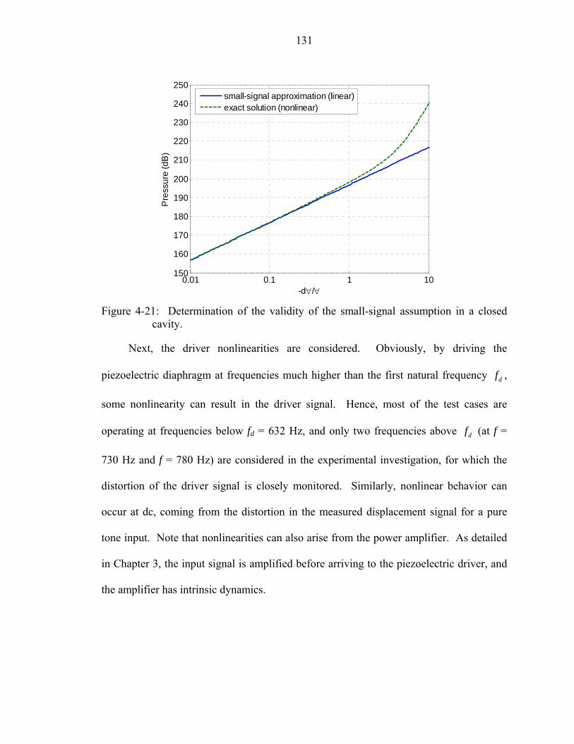
131

0.01 0.1 1 10150

160

170

180

190

200

210

220

230

240

250

-d∀/∀

Pre

ssur

e (d

B)

small-signal approximation (linear)exact solution (nonlinear)

Figure 4-21: Determination of the validity of the small-signal assumption in a closed

cavity.

Next, the driver nonlinearities are considered. Obviously, by driving the

piezoelectric diaphragm at frequencies much higher than the first natural frequency df ,

some nonlinearity can result in the driver signal. Hence, most of the test cases are

operating at frequencies below fd = 632 Hz, and only two frequencies above df (at f =

730 Hz and f = 780 Hz) are considered in the experimental investigation, for which the

distortion of the driver signal is closely monitored. Similarly, nonlinear behavior can

occur at dc, coming from the distortion in the measured displacement signal for a pure

tone input. Note that nonlinearities can also arise from the power amplifier. As detailed

in Chapter 3, the input signal is amplified before arriving to the piezoelectric driver, and

the amplifier has intrinsic dynamics.

132

10-5

10-4

10-3

10-2

10-1

10-6

10-4

10-2

100

102

104

d∀/∀

THD

in ∆

Pc (%

)

S=4S=12S=14S=17S=43S=53

0 0.5 1 1.5 2 2.5 3 3.510

-6

10-4

10-2

100

102

104

ω/ωH

THD

in ∆

Pc (%

)

S=4S=12S=14S=17S=43S=53

Figure 4-22: Log-log plot of the cavity pressure total harmonic distortion in the

experimental time signals. A) Versus d∀ ∀ . B) Versus Hω ω .

After being identified, these nonlinearities must also be extracted and quantified to

determine their effect on the actuator behavior. A useful tool in the investigation of

nonlinear effects is found in the study of the total harmonic distortion (THD). The THD

is defined as the ratio of the sum of the powers of all harmonic frequencies above the

fundamental frequency to the power of the fundamental one (National Instruments 2000):

A

B

133

( ) ( )( ) ( )1

0

THD % 100N

kkG

Gω

ω== ×∑ , (4-14)

where k = 1…N is the number of harmonics and k = 0 represents the fundamental

frequency. The results of the spectral analysis of the time signal presented in Chapter 3

are used in this investigation. Note that in this analysis the THD contains the measured

total harmonic distortion up to and including the highest harmonic at 10ω (N = 10), hence

is not limited to the first few harmonics. First, Figure 4-22 shows the THD present in the

cavity pressure (taken with microphone 1, see Chapter 3 for definition) as a function of

the change in the cavity volume d∀ ∀ and function of the ratio of the Helmholtz to

actuation frequency Hω ω . Clearly, the distortions in the cavity pressure signal are not

affected by the change in cavity volume, as shown in Figure 4-22A and described above.

Similarly, compressibility effects appear to not play a role in the cavity pressure signal

distortion, as seen from Figure 4-22B. The next chapter (Chapter 5) discusses the cavity

compressibility effect in more details.

Next, Figure 4-23 shows the THD variation in the time signals as a function of the

Strouhal number for different Stokes numbers. From the pressure signal (acquired by

microphone 1, see Figure 3-3 in Chapter 3 for definition) plotted in Figure 4-23A,

significant nonlinearities are present especially at the low Strouhal number cases. This is

in accordance with the time traces already seen in Figure 3-1. . Figure

4-23B shows the THD in the jet volume velocity which, besides a few cases at low

Strouhal numbers, is less than 1%. This means that the majority of the cases can have jQ

accurately represented by a pure sinusoidal signal. Finally, the THD present in the

diaphragm signal is shown in Figure 4-23C. Clearly, the motion of the diaphragm

134

displacement in time can be correctly assumed to be sinusoidal for all the cases

considered, a negligible percent of nonlinearities in the signal being present. Therefore,

practically the nonlinearities present in the experimental signal mostly come from the

orifice, no cases are found to be strongly affected by nonlinearities that are not due just to

the orifice.

10-2

10-1

100

101

102

10-6

10-4

10-2

100

102

104

St

THD

in ∆

Pc (%

)

S=4S=12S=14S=17S=43S=53

10-2

10-1

100

101

102

10-2

10-1

100

101

St

THD

in Q

j (%)

S=4S=12S=14S=17S=43S=53

Figure 4-23: Log-log plot of the total harmonic distortion in the experimental time

signals vs. Strouhal number as a function of Stokes number. A) Cavity pressure. B) Jet volume flow rate. C) Driver volume flow rate.

A

B

135

10-2

10-1

100

101

102

10-3

10-2

10-1

100

101

St

THD

in Q

d (%)

S=4S=12S=14S=17S=43S=53


To summarize this chapter, a joint experimental and numerical investigation of the

velocity profiles, at the orifice exit as well as inside the orifice, has been performed.

Numerical simulations are a useful tool to elucidate the orifice flow physics in ZNMF

actuators and complement the experimental results. Clearly, the orifice flow is far from

trivial, especially for such small orifices and flow conditions, and it exhibits a rich and

complex behavior that is a function of the location inside the orifice and a function of

phase angle during the cycle.

Next, the influence of the governing parameters, such as the orifice aspect ratio h/d,

Stokes number S, Reynolds number Re, Strouhal number St, or stroke length L0, has been

experimentally and numerically investigated. It has been found that a dimensionless

stroke length – equivalent to the Strouhal number times h/d - is the main parameter in

describing the losses associated with the pressure drop across the orifice.

Finally, a survey of the possible sources of nonlinearities present in the time signals

of interest (pressure, jet volume flow rate) has been performed. Potential nonlinear

C

136

sources were identified and evaluated; their overall influence on the actuator performance

has been quantified through a total harmonic distortion analysis. The information

gathered through this study on the orifice flow results will aid in the understanding and

the development of a physics-based reduced-order model of such actuators in subsequent

chapters.

137

CHAPTER 5

RESULTS: CAVITY INVESTIGATION

This chapter discusses the cavity behavior of a ZNMF actuator device, based on the

experimental results presented in the previous chapter and using available numerical

simulation results. A discussion is first provided on the measured and computed cavity

pressure field, based on experimental and numerical results. Then follows a careful

analysis of the compressibility effects occurring inside the cavity where it is shown that

the Helmholtz frequency is the critical parameter to be considered. Finally, the driver,

cavity and jet volume velocities are considered, specifically their respective roles and

how they interact and couple with each other. Ultimately, this investigation on the cavity

will give valuable insight and help in the understanding of the physical behavior of

ZNMF actuators in quiescent air for both modeling and design purposes.

Cavity Pressure Field

The knowledge of the pressure inside the cavity is of great interest since it dictates

the orifice flow behavior, which is naturally a pressure-driven oscillatory flow. In fact,

the cavity pressure fluctuations are approximately equivalent to the pressure drop across

the orifice; hence it plays a central role in the overall actuator response. Specifically, the

magnitude and the phase of the pressure signal are of interest, and comparing the data

from two separate microphones placed at different locations inside the cavity, as shown

in Figure 3-3, provide some answers. Moreover, since a characteristic feature of the

reduced-lumped element model presented in Chapter 2 is to assume that the pressure drop

across the orifice is equivalent to the cavity pressure, it is of great importance to know

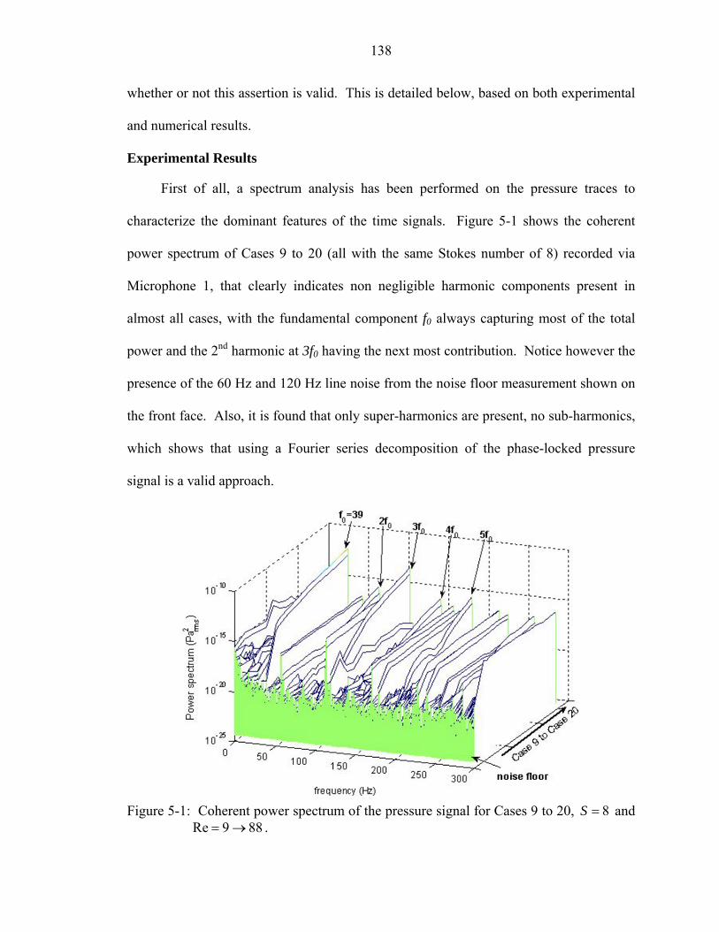
138

whether or not this assertion is valid. This is detailed below, based on both experimental

and numerical results.

Experimental Results

First of all, a spectrum analysis has been performed on the pressure traces to

characterize the dominant features of the time signals. Figure 5-1 shows the coherent

power spectrum of Cases 9 to 20 (all with the same Stokes number of 8) recorded via

Microphone 1, that clearly indicates non negligible harmonic components present in

almost all cases, with the fundamental component f0 always capturing most of the total

power and the 2nd harmonic at 3f0 having the next most contribution. Notice however the

presence of the 60 Hz and 120 Hz line noise from the noise floor measurement shown on

the front face. Also, it is found that only super-harmonics are present, no sub-harmonics,

which shows that using a Fourier series decomposition of the phase-locked pressure

signal is a valid approach.

Figure 5-1: Coherent power spectrum of the pressure signal for Cases 9 to 20, 8S = and

Re 9 88= → .

139

Figure 5-2: Phase plot of the normalized pressures taken by microphone 1 versus

microphone 2. A) Case 46. B) Case 49. C) Case 59. D) Case 62.

Next, the phase difference between the two microphones is analyzed. Four

different cases are examined, one when the two pressure signals appear quite sinusoidal

and similar in shape as in Case 46 ( )Re 109, 26St= = and Case 49 ( )Re 1439, 2St= = ,

another one (Case 59, Re 3039, 0.9St= = ) when one microphone exhibits some

distortion while the other is rather sinusoidal, and finally the scenario when both signals

are clearly nonlinear, as in Case 62 ( )Re 157, 0.1St= = . Figure 5-2 shows the phase

plots of these four cases, where the pressure data is normalized by subtracting the mean

µ and dividing by the standard deviation σ . Cleary, in each scenario the phase between

the two microphones is surprisingly invariant, with the exception of Case 59. And

( )Re 157, 0.1St= =( )Re 3039, 0.9St= =

( )Re 109, 26St= = ( )Re 1439, 2St= =

A B

C D

140

although only four cases are reported here, this behavior is typical for all cases. As for

Case 59, Figure 5-3 plots the phase locked pressure signals during one cycle, and the

phase difference observed from the phase plot is clearly seen here when crossing the zero

axis, but the peak amplitudes occur at the same phase for each signal, i.e. at the maximum

expulsion and maximum ingestion time of the cycle.

0 45 90 135 180 225 270 315 360-800

-600

-400

-200

0

200

400

600

800

phase (degree)

Pre

ssur

e (P

a)

Microphone 1

Microphone 2

Figure 5-3: Pressure signals experimentally recorded by microphone 1 and microphone 2

as a function of phase in Case 59 ( )53, Re 3039, 0.9S St= = = .

The amplitude of the pressure inside the cavity is investigated next. While the

phase seems spatially invariant inside the cavity, a change in amplitude is noted. This is

already seen in Figure 5-3 for Case 59, but is also represented for all cases in Figure 5-4

that plots the ratio of the total amplitude between microphone 2 and 1, as a function of

the inverse of the Strouhal number. Noticeably, referring to Figure 3-3 for the

microphone locations, whether the pressure amplitude is recorded on the side or on the

bottom of the cavity does matter. Notice that by plotting ,2 ,1c cP P∆ ∆ against 1 St , one

can also infer the influence of the jet formation criterion on the pressure data. Certainly,

141

whether a jet is formed or not may affect the pressure amplitude variation inside the

cavity. Moreover, when looking at the value of kH - the wavenumber times the largest

cavity dimension - for these cases, and indicated in the legend of Figure 5-4, it is clear

that for the high Stokes number cases, the compact acoustic source approximation may

not be valid anymore, meaning that the cavity does not act like a pure compliance and

some mass, or inertia, terms may come into play.

10-2

10-1

100

101

102

0.2

0.4

0.6

0.8

1

1.2

1.4

1/St

∆P

c, 2

/ ∆

Pc,

1

S=4, kH=0.029S=12, kH=0.029S=14, kH=0.37S=17, kH=0.55S=43, kH=0.37S=53, kH=0.58

No jet Jet

Figure 5-4: Ratio of microphone amplitude (Pa) vs. the inverse of the Strouhal number,

for different Stokes number. The vertical line indicates the jet formation criterion.

Numerical Simulation Results

Numerical simulations are a useful tool, especially when experiments fail. Indeed,

in the present context it is really difficult, if not impossible, to measure the actual

pressure drop across the orifice - hence the two microphones placed inside the cavity.

Therefore, the importance of the CFD results takes its entire place for cavity flows.

142

Computational fluid dynamics

To confirm the experimental observations, available numerical simulation data is

thus analyzed. These data have been previously reported in Gallas et al. (2004), the

methodology for the numerical simulations is given in Appendix F, and Case 2

( )Re 262, 2.4St= = and Case 3 ( )Re 262, 0.4St= = in the test matrix (Table 2-3) are

considered here. Notice however that this simulation uses an incompressible solver for

the cavity where the pressure field is computed by solving the Poisson equation, and that

it assumes a 2D sinusoidal vibrating membrane at the bottom of the cavity, thereby

neglecting any three-dimensional effects. Yet the solution can be considered valid since

the actuation frequency is far below the Helmholtz frequency (the next section describes

this compressibility effect in great detail), and since the cavity size is much smaller than

the wavelength. Also, previous work (Utturkar et al. 2002) showed that the ZNMF

actuator performance was rather insensitive to the driver placement inside the cavity.

The pressure distribution at one instant in time is first given for Case 2, where

Figure 5-5A corresponds to 45o during the expulsion portion of the cycle (0o

corresponding to the onset of jet expulsion), and Figure 5-5B is at the beginning of the

ingestion cycle. In this case where no jet is formed, the pressure is fairly uniform inside

the cavity away from the orifice entrance. On the other hand, in the case where a clear jet

is formed, as for Case 3, the pressure inside the cavity has a more disturbed pattern, as it

can be seen in Figure 5-6 where contours of the pressure field is shown at different

phases during the ingestion portion of the cycle. Nodes are present inside the cavity as a

function of phase, which is mainly due to the high stroke length that is characteristic of

this case. During the ingestion process, fluid particle reach and impinge on the bottom of

143

the cavity, hence generating some circulation at the corners that quickly dissipates as the

driver starts a new cycle.

Figure 5-5: Pressure contours in the cavity and orifice for Re 262= and 2.4St = (Case 2) from numerical simulations. A) 45o during expulsion. B) Beginning of the suction cycle, referenced to Qj.

phase

Qj

180o0o 360o

expulsion ingestion

A

phase

Qj

180o0o 360o

expulsion ingestion

B

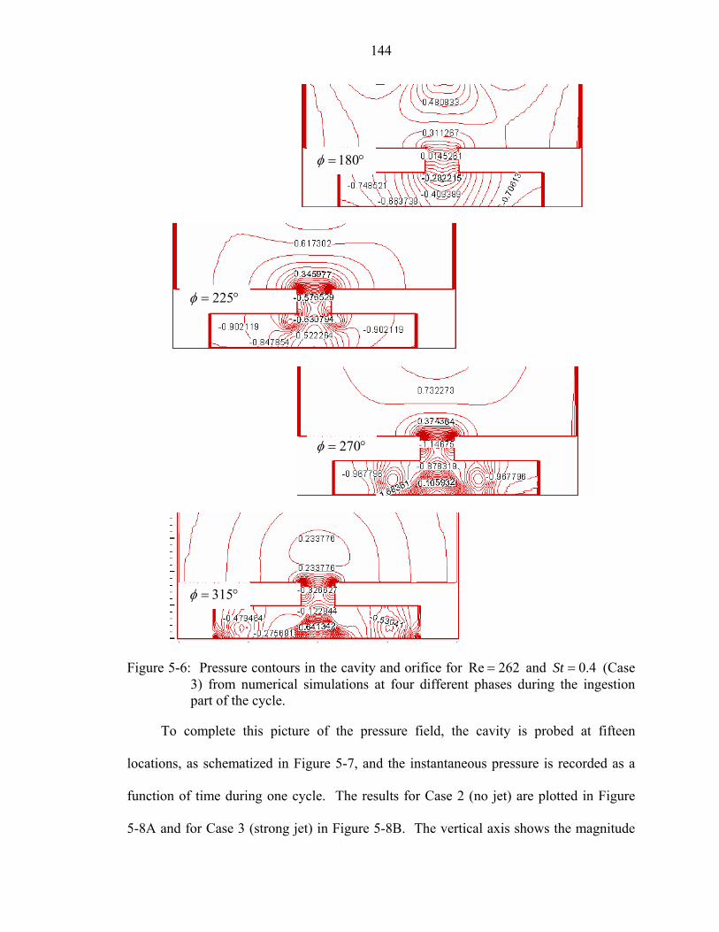
144

Figure 5-6: Pressure contours i3) from numerical spart of the cycle.

To complete this picture

locations, as schematized in Fig

function of time during one cyc

5-8A and for Case 3 (strong jet)

180φ = °

225φ = °

315φ = °

270φ = °

n the cavity and orifice for Re 262= and 0.4St = (Case imulations at four different phases during the ingestion

of the pressure field, the cavity is probed at fifteen

ure 5-7, and the instantaneous pressure is recorded as a

le. The results for Case 2 (no jet) are plotted in Figure

in Figure 5-8B. The vertical axis shows the magnitude

145

of the pressure normalized by 2

jVρ , on one of the horizontal axes is the phase angle and

on the other one the five slices corresponding to the five cuts made parallel to the driver

up to the orifice inlet, as schematized in Figure 5-7. For each slice, the side, middle and

center probes are plotted on top of each other. In these two examples, the effect of a jet

being formed at the orifice exit, and hence at the orifice inlet as well, does appear to

influence the pressure field inside the cavity.

centerprobes

middleprobes

sideprobes

orifice

driver

X XX

X XX

X XX

X XX

X XX

X pressure probe

Figure 5-7: Cavity pressure probe locations in a ZNMF actuator from numerical

simulations.

Actually, to try comparing the CFD data with the experimental results, although the

driver is not on the same side of the cavity and is modeled as a 2D vibrating membrane,

the three locations corresponding to the positions of the two microphones in the

experimental setup plus just at the orifice entrance are extracted from the above figures

and are shown in Figure 5-9. Clearly, as one move towards the orifice, the pressure

decreases and increasing distortion in the time signals are noted for the large stroke

length case. Also, the pressure is much larger in amplitude for the higher Stokes number

case, although the two cases have the same jet Reynolds number. Note that the phase

between the different pressure probes is again spatially invariant.

146

Figure 5-8: Normalized pressure inside the cavity during one cycle at 15 different probe locations from numerical simulation results. A) Case 2 (no jet formed). B) Case 3 (jet formed).

A

B

147

Figure 5-9: Cavity pressure normalized by

2

jVρ vs. phase from numerical simulations corresponding to the experimental probing locations. A) Case 2 (no jet formed). B) Case 3 (jet formed).

Femlab

Finally, a simple calculation was also performed in FEMLAB to check the pressure

field inside the cavity. The geometry of the device utilized in the experiments is used to

construct a 3D simulation. A time-harmonic analysis is then applied on the meshed

domain that solve the Helmholtz equation

2

20

1 0pp qc

ωρ ρ

⎛ ⎞∇ ⋅ − ∇ + − =⎜ ⎟

⎝ ⎠, (5-1)

where q is a dipole source. Sound hard boundaries are applied on the walls (normal

derivative of the pressure is zero on the boundary), an impedance boundary condition is

prescribed at the orifice exit that is based on the experimental results, and the diaphragm

is simply modeled as an accelerating boundary in an harmonic manner, the three-

dimensional mode shape being modeled via a Bessel function (representative of the

solution of the wave equation for a clamped membrane). The steady state wave equation

is then solved for a specified driving frequency, i.e. the pressure p is equal to i tpe ω . Note

(a) (b) 0 45 90 135 180 225 270 315 360

-15

-10

-5

0

5

10

15

phase

Microphone 1Microphone 2Orifice entrance

0 45 90 135 180 225 270 315 360-1.5

-1

-0.5

0

0.5

1

1.5

2

2.5

phase


Re 262, 0.4St= = Re 262, 2.4St= =

A B

Normalized pressure Normalized pressure

148

that even though the orifice is present in the geometry, viscous effects are completely

ignored and only the acoustic field is considered. Two experimental cases are simulated,

namely Case 55 ( )39f Hz= and Case 58 ( )780f Hz= .

Figure 5-10: Contours of pressure phase inside the cavity by numerically solving the 3D

wave equation using FEMLAB. A) Case 55. B) Case 58.

The results are shown in Figure 5-10 and Figure 5-11, where Figure 5-10 shows the

contour plot of the pressure phase inside the cavity which can be seen to be invariant

throughout the entire domain. Similarly, Figure 5-11 shows the pressure amplitude

versus phase for the probe points that correspond to the locations of the microphones, as

well as the point right at the orifice inlet, in the same manner as described above in

Figure 5-9. Clearly, the pressure is fairly uniform at these two driving frequencies, f = 39

Hz and f = 780 Hz. It should be pointed out that the pressure recorded here does not

match the experimental results since this simulation is kept at a simple level, bypassing

the complex structural and fluidic interactions that occur in the real device, only the wave

equation being solved here. The all point of this exercise is to infer the uniformity of the

max = 2.534min = 2.541

max = 2.637min = 2.275

39f Hz= 780f Hz=

A B

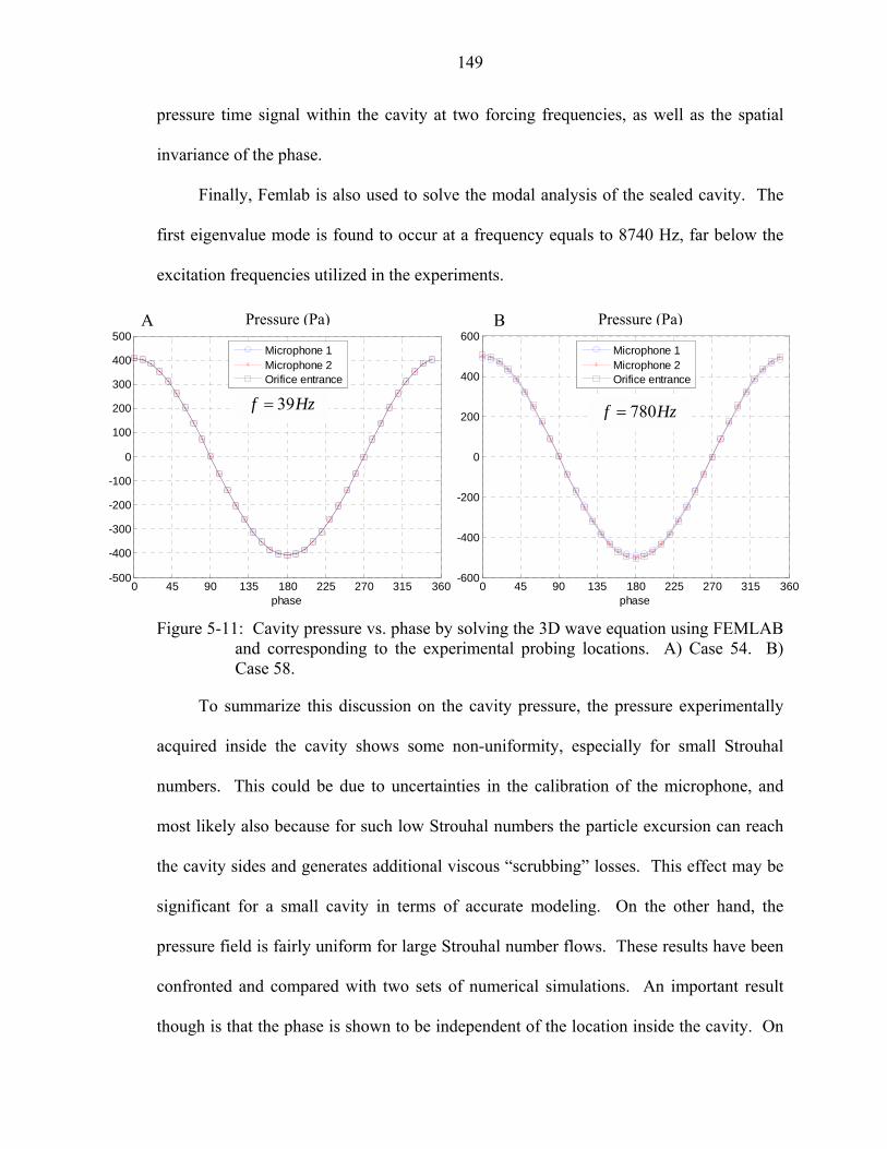
149

pressure time signal within the cavity at two forcing frequencies, as well as the spatial

invariance of the phase.

Finally, Femlab is also used to solve the modal analysis of the sealed cavity. The

first eigenvalue mode is found to occur at a frequency equals to 8740 Hz, far below the

excitation frequencies utilized in the experiments.

Figure 5-11: Cavity pressure vs. phase by solving the 3D wave equation using FEMLAB

and corresponding to the experimental probing locations. A) Case 54. B) Case 58.

To summarize this discussion on the cavity pressure, the pressure experimentally

acquired inside the cavity shows some non-uniformity, especially for small Strouhal

numbers. This could be due to uncertainties in the calibration of the microphone, and

most likely also because for such low Strouhal numbers the particle excursion can reach

the cavity sides and generates additional viscous “scrubbing” losses. This effect may be

significant for a small cavity in terms of accurate modeling. On the other hand, the

pressure field is fairly uniform for large Strouhal number flows. These results have been

confronted and compared with two sets of numerical simulations. An important result

though is that the phase is shown to be independent of the location inside the cavity. On

0 45 90 135 180 225 270 315 360-600

-400

-200

0

200

400

600

phase

Pre

ssur

e (P

a)


0 45 90 135 180 225 270 315 360-500

-400

-300

-200

-100

0

100

200

300

400

500

phase


39f Hz= 780f Hz=

Pressure (Pa) Pressure (Pa) A B

150

the contrary, the amplitude of the pressure fluctuations does depend on the probe

location, and the pressure amplitude just at the orifice entrance seems to be always

slightly different than anywhere else inside the cavity. In fact, the microphones are

measuring not only the dynamic pressure fluctuation due to the oscillating flow within

the orifice, but also any hydrodynamics and acoustics effects, such as radiation. This fact

has to be taken into account for impedance estimation of the orifice since LEM assumes

an equal pressure inside the cavity to that across the orifice. In practice, one should place

the microphones in a similar way to what is commonly employed in tabulated orifice

flow meters that use corner pressure tap (White 1979). Therefore, the quantitative

experimental results based on the cavity pressure should be considered with cautious.

Compressibility of the Cavity

The question of the validity of an incompressible assumption for modeling the

cavity is of great interest and practical importance. First, from a computational point of

view, it is rather essential to know whether the flow inside the cavity can be considered

as incompressible, the computational approach being quite different for a compressible

and an incompressible solver. Second, from the equivalent circuit perspective of the

lumped element model presented in Chapter 2, a high cavity impedance (which occurs for

a “stiff” or incompressible cavity) will prevent the flow from going into the cavity

branch. On the other hand, a “compliant” or compressible cavity will draw fluid flow

hence reducing the output response. The compressibility behavior is explored via

illustrative cases, both analytically and experimentally. The LEM prediction serves in

providing the general trend and behavior in the frequency domain, while experimental

data are used here to validate these findings.

151

LEM-Based Analysis

First, consider some analytical examples. They are Case 1 described in Gallas et al.

(2003a) and Case 1 of the NASA Langley workshop CFDVal2004 (2004). Both

examples have a piezoelectric-diaphragm driver and are thus expected to exhibit two

resonant frequencies. The acoustic impedance of the cavity aCZ is systematically varied

through the cavity volume variable ∀ since, assuming an isentropic ideal gas, they are

directly related via

201

aCaC

cZj C j

ρω ω

= =∀

, (5-2)

and the frequencies that govern the system response are recorded and compared. From

Eq. 5-2, it is expected that as the cavity volume decreases and tends to zero, the acoustic

compliance aCC also tends to zero, and the cavity becomes “stiff”. These frequencies are

defined as follows. In particular, 1f and 2f are the first and second resonance

frequencies, respectively, in the synthetic jet frequency response and are defined in

Gallas et al. (2003a)

( )2 2 2 2 21 0d H d Hf f f fψ ψ⎡ ⎤− + + + =⎣ ⎦C , (5-3)

where aD aCC C=C is the compliance ratio, and 2ifψ = . The two roots of the quadratic

equation Eq. 5-3 are the square of the natural frequencies of the synthetic jet, i.e. 21f and

22f . Here, 2H Hf ω π= is the Helmholtz frequency of the synthetic jet resonator and

since

1H

aO aCM Cω = , (5-4)

152

is directly proportional to the cavity and orifice geometrical dimensions via both the

acoustic mass of the orifice aOM and the acoustic compliance of the cavity aCC ∝∀ (see

Eq. 5-2). Similarly, 2d df ω π= is the natural frequency of the actuator diaphragm. In

general 1 or H df f f≠ and 2 or d Hf f f≠ , and only for the limiting cases when 1f and 2f

are widely separated in frequency do the two peaks approach the driver and Helmholtz

frequencies. Nevertheless, these two frequencies are always constrained via 1 2 d Hf f f f= .

With this information as background, consider Case 1 from Gallas et al. (2003a), in

which all parameters are fixed to their respective nominal values and the cavity volume is

progressively decreased. The baseline case is such that H df f< , and the natural

frequency of the diaphragm along with the orifice dimensions are held constant.

Table 5-1 shows the impact of the decrease of the cavity volume on the frequency

response of the system, and is illustrated in the log-log plot in Figure 5-12. The first

frequency 1f is clearly governed by the diaphragm natural frequency and tends to a fixed

value equal to df as the volume decreases, while the second frequency 2f is influenced

by the Helmholtz frequency Hf that tends to infinity as the volume is decreased. Notice

however that LEM breaks down for high frequencies since the assumption of 1kd is

no longer valid.

153

Table 5-1: Cavity volume effect on the device frequency response for Case 1 (Gallas et al. 2003a) from the LEM prediction.

( )2114df Hz= ( )Hf Hz ( )1f Hz ( )2f Hz

Baseline: ( )6 30 2.5 10 m−∀ = × 941 918 2,167

0 2∀ =∀ 1,331 1,254 2,243

0 5∀ =∀ 2,104 1,685 2,640

0 10∀ =∀ 2,976 1,832 3,434

0 20∀ =∀ 4,208 1,885 4,719

0 50∀ =∀ 6,654 1,911 7,363

0 100∀ =∀ 9,410 1,918 10,372

0 500∀ =∀ 21,042 1,924 23,123

0 1000∀ =∀ 29,757 1,924 32,690

100

101

102

103

104

105

10-2

10-1

100

101

102

Frequency (Hz)

Cen

terli

ne v

eloc

ity (m

/s)

∀0=2.6e-6 m3

∀=∀/5∀=∀/100∀=∀/100

fd

+20 dB / d

ecade

-20 dB/decade

-60 dB/decade

∀ ↓

Figure 5-12: Log-log frequency response plot of Case 1 (Gallas et al. 2003a) as the cavity volume is decreased from the LEM prediction.

154

Table 5-2: Cavity volume effect on the device frequency response for Case 1 (CFDVal 2004) from the LEM prediction.

( )460df Hz= ( )Hf Hz ( )1f Hz ( )2f Hz

Baseline: ( )6 30 7.4 10 m−∀ = × 1,985 446.2 2,048

0 2∀ =∀ 2,808 446.5 2,894

0 5∀ =∀ 4,440 446.7 4,574

0 10∀ =∀ 6,279 446.8 6,468

0 20∀ =∀ 8,880 446.8 9,146

0 50∀ =∀ 14,044 446.9 14,461

0 100∀ =∀ 19,856 446.8 20,451

0 500∀ =∀ 44,400 446.8 45,729

0 1000∀ =∀ 62,791 446.8 64,671

100

101

102

103

104

105

10-4

10-3

10-2

10-1

100

101

102

Frequency (Hz)

Cen

terli

ne v

eloc

ity (m

/s)

∀0=2.6e-6 m3

∀=∀/5∀=∀/100∀=∀/1000

fd

+20dB/decade

-60dB/decade

∀ ↓

-20dB/decade

Figure 5-13: Log-log frequency response plot of Case 1 (CFDVal 2004) as the cavity volume is decreased from the LEM prediction.

155

Similarly, as a second example, all parameters are based on Case 1 of the NASA

workshop CFDVal2004 (2004), and the cavity volume is again progressively decreased

from its nominal value. This time, the baseline case is such that H df f> , and Table 5-2

and Figure 5-13 are generated to illustrate the behavior of the actuator frequency

response. In this case, the first resonant frequency is governed by the cavity resonant

frequency Hf that tends to infinity as the cavity volume is decreased, while the second

frequency is limited by the natural frequency of the diaphragm df . This case is actually

the continuation of the previous example but starting with Hf already greater than df ,

hence starting with a smaller cavity.

Interestingly, in both cases the system exhibits a 20 dB/decade rise at low

frequencies, and has a -60 dB/decade roll off at high frequencies representative of a

system with a pole-zero excess of 3. In between the two resonant frequencies 1f and 2f ,

the response decreases at a rate of 20 dB/decade, similar to a 1st-order system. The

influence of the cavity volume is clearly confined to one of the peaks in the actuator

response. For both cases, as the cavity volume shrinks to zero, a single low frequency

peak near the diaphragm natural frequency is obtained. The second peak progressively

moves to higher frequencies as the cavity volume is decreased, and since 1Hf ∝ ∀ the

following limit behavior is observed

( )( )

10

20

lim

lim

d

H

f f

f f∀→

∀→

→⎧⎪⎨

→ →∞⎪⎩. (5-5)

156

Experimental Results

This interesting behavior is now experimentally verified. In the experimental

investigation described in Chapter 3, this is referred to as Test 2 in the setup. A nominal

synthetic jet device is taken and the cavity volume is systematically decreased to yield

four different actuators, with all other components held fixed. The dimensions and test

conditions of the devices are listed in Table 3-1. The phase-locked centerline velocity is

then acquired at different frequencies using LDV measurements, in the same manner as

discussed in Chapter 3.

Table 5-3: ZNMF device characteristic dimensions used in Test 2 Property: Case A Case B Case C Case D Cavity volume ∀ (m3) 4.49×10-6 2.42×10-6 1.09×10-6 0.71×10-6 Orifice diameter d (mm) 1.5 Orifice thickness h (mm) 2.7 Orifice width w (mm) 11.5 Diaphragm diameter (mm) 23 Input sine voltage acV (Vpp) 30 Diaphragm natural frequency

df (Hz) 2114

Helmholtz frequency Hf (Hz) * 1275 1738 2586 3221

(*) computed from Eq. 5-6

The results are plotted in a log-log scale in Figure 5-14 and Figure 5-15 gives a

close-up view of the peak locations in a linear plot. Also, Table 5-4 lists the different

frequencies of interest. Two sets of frequencies are compared: ones that are

experimentally measured, the others that are analytically computed. The frequency

response plot in Figure 5-15 provides 1,expf and 2,expf the two natural frequencies of the

system. For the two test cases that have a cavity wide enough to allow the insertion of a

microphone inside (Case A and Case B), the Helmholtz frequency is experimentally

determined by a simple “blowing test” (effect of blowing over an open bottle) where the

157

spectra of the microphone is recorded while the actuator is passively excited by blowing

air at the orifice lip. Then, analytically 1f and 2f are computed solving Eq. 5-3 that only

requires the knowledge of the diaphragm and cavity acoustic compliances and df and

Hf . Here, Hf is calculated from its acoustical definition, i.e.,

( )0

0

12

nH

Sf ch hπ

=+ ∀

, (5-6)

where 0 0.96 nh S= is the orifice effective length for an arbitrary aperture (see Appendix

B). Note also that in this experimental setup, the largest dimension of the device is the

cavity height H equals to 26.8mm. The frequency limit under which Eqs. 5-4 and 5-6 are

still valid corresponds to about 1kH < , or 1/ 6H λ < . In terms of frequency, this means

that the LEM assumption in these test cases is only valid for frequencies 2200f Hz< ,

i.e. about up to the natural frequency of the diaphragm. And clearly, as seen in Table 5-4,

this assumption is violated for the 2 smallest cavities, hence the discrepancy between the

experimental and analytical 1f and 2f .

Table 5-4: Effect of the cavity volume decrease on the ZNMF actuator frequency response for Cases A, B, C, and D.

from experiments from analytical equations

( )2114df Hz= ( )Hf Hz ( )1f Hz ( )2f Hz ( )Hf Hz ( )1f Hz ( )2f Hz

Case A 1272 1200 2100 1275 1253 2152

Case B 1732 1600 2000 1738 1651 2226* Case C N/A 1700 2400 2586* 1972 2774* Case D N/A 1700 2600 3221* 2014 3383*

* LEM assumption no longer valid: lim, 2200LEMf Hz≈

158

101

102

103

10-3

10-2

10-1

100

101

Frequency (Hz)

fd

∀ = 4.49 x 10-6 m3

∀ = 2.42∀ = 1.09∀ = 0.71

Cen

terli

ne v

eloc

ity a

mpl

itude

(m/s

)

Figure 5-14: Experimental log-log frequency response plot of a ZNMF actuator as the

cavity volume is decreased for a constant input voltage.

1000 1500 2000 2500 3000

2

6

10

13

Frequency (Hz)

Cen

terli

ne v

eloc

ity a

mpl

itude

(m/s

) fd fH, DfH, A fH, B fH, C

Figure 5-15: Close-up view of the peak locations in the experimental actuator frequency

response as the cavity volume is decreased for a constant input voltage. The arrows point to the analytically determined Helmholtz frequency Hf for each case. ( ) Case A: 6 34.49 10 m−∀ = × , ( ) Case B: 6 32.42 10 m−∀ = × , ( ) Case C: 6 31.09 10 m−∀ = × , ( ) Case D: 6 30.71 10 m−∀ = × .

159

An identical behavior seen in the lumped element model applied above for the two

examples is seen in the results. First the overall dynamic response is still characterized

by a +20 dB/decade rise at the low frequencies and -60 dB/decade roll off for the high

frequencies. Also, the system response exhibits two frequency peaks. Figure 5-15 shows

a close-up view of the peak locations, where the arrows indicate the Helmholtz frequency

location given by Eq. 5-6. As the cavity volume decreases, Hf increases while df

remains constant. Also, if 1H df f < , Hf is easily distinguished from df (as in Case A

or Case B), and the actual peak frequencies 1f and 2f are close to Hf and df . However,

when 1H df f ∼ , the experimentally determined peaks 1f and 2f tend to move away

from df (Case C and Case D). As H df f→ , 1f and 2f approach each other. Then as

Hf exceeds df , they separate again, and eventually 1f tends to df . Then, as the cavity

volume is further decreased, 2f and the Helmholtz frequency move toward higher

frequencies, while 1f tends to df , as in Case D. Notice also how the frequency response

is unaffected by the cavity size -hence compressibility effects- for frequencies smaller

than Hf of Case A, as seen in Figure 5-14. This suggests that their exists a threshold

limit below which the actuator response is independent of the Helmholtz frequency, or

for 0.5Hf f < .

To further confirm this trend experimentally, a smaller cavity size would have been

ideal, but physical constraints in the actuator configuration prevented it; Case D already

has the smallest feasible cavity. Nonetheless, the experimental results validate the

lumped element model analysis presented above, where a similar change in the frequency

160

response of a ZNMF actuator occurs due to the cavity volume variation, hence affecting

the Helmholtz frequency peak location, as described by Eq. 5-5.

Figure 5-16: Normalized quantities vs. phase of the jet volume rate, cavity pressure and

centerline driver velocity. A) Case 20: Re 102, 7S= = . B) Case 70: Re 50, 4S= = . C) Case 46: Re 109, 53S= = . D) Case 65: Re 269, 17S= = .

Actually, the results from Test 1 described in Chapter 3 where the pressure

fluctuations are recorded inside the cavity can also give additional proof in the above

analysis. This is shown in Figure 5-16 where the normalized jet volume flow rate, cavity

0 50 100 150 200 250 300 350

-1

-0.8

-0.6

-0.4

-0.2

0

0.2

0.4

0.6

0.8

1

phase

0 50 100 150 200 250 300 350

-1

-0.8

-0.6

-0.4

-0.2

0

0.2

0.4

0.6

0.8

1

phase

0 50 100 150 200 250 300 350

-1

-0.8

-0.6

-0.4

-0.2

0

0.2

0.4

0.6

0.8

1

phase

0 50 100 150 200 250 300 350

-1

-0.8

-0.6

-0.4

-0.2

0

0.2

0.4

0.6

0.8

1

phase

Vd ∆PcavQj

A

C 0.86Hf f = 3.28Hf f =

0.09Hf f =0.06Hf f =

D

B

161

pressure and driver centerline velocity are plotted phase-locked for four different Hf f

ratios. Notice that in these plots the small errobars are omitted for better illustration. For

cases actuated at a frequency away from the Helmholtz frequency, as seen in Figure

5-16A and Figure 5-16B, the volume flow rate and centerline driver velocity are nearly in

phase, indicating that the flow is incompressible. In contrast, for cases of driver

frequencies close to or greater than Hf as in Figure 5-16C and Figure 5-16D, the orifice

volume flow rate is not in phase with the driver velocity, ostensibly due to

compressibility effects in the cavity. If the flow in the cavity is incompressible, it has the

effect of not delaying the time signals.

The driver-to-Helmholtz frequency ratio Hf f is thus the key parameter in this

analysis. Recall from Eq. 5-2 and Eq. 5-4 that a small cavity volume with a large

Helmholtz frequency is equivalent to having an incompressible cavity. Therefore, if the

actuation frequency of the ZNMF actuator is well below its Helmholtz frequency, the

flow within the cavity of the device can be treated as incompressible, whereas if the

actuator is excited near its Helmholtz frequency or above some critical frequency

0.5Hf f > , certainly the flow inside the cavity is compressible, which then has to be

consistently considered for modeling purposes. This is an important result that can be

summarized by stating that

0.5 incompressible cavity

otherwise compressible cavityH

ff

⎧ < ⇒⎪⎨⎪ ⇒⎩

(5-7)

This criterion should be taken into account for numerical simulations and design

considerations.

162

Driver, Cavity, and Orifice Volume Velocities

The previous analysis shows the impact of the actuation to Helmholtz frequency

ratio Hf f on the frequency response of a ZNMF actuator in quiescent air that results in

a criterion for the cavity incompressibility limit. However, more results can be extracted

from this experimental investigation in terms of the actuator response magnitude. As

suggested from Figure 5-14, the variation in amplitude of the jet velocity is a direct

function of the Helmholtz frequency. To have a first estimate of these variations, the

dimensionless linear transfer function derived in Chapter 2 for a generic driver and

orifice (see Eq. 2-23) that gives a scaling argument for j dQ Q is considered and

reproduced below:

( )

22

1

11

j j

d

H H

Q QQ j

jS

ωω ω ω

ω ω

= ≈∆∀ ⎡ ⎤ ⎡ ⎤⎛ ⎞ ⎛ ⎞

− +⎢ ⎥ ⎢ ⎥⎜ ⎟ ⎜ ⎟⎢ ⎥⎝ ⎠ ⎝ ⎠⎣ ⎦⎣ ⎦

. (5-8)

Recall that this expression used Eq. (5-4) to define the Helmholtz frequency, hence

neglecting the radiation mass that results in an effective length. Also, Eq. 5-8 was

derived assuming a linear model, neglecting any nonlinear resistance terms. Yet this

expression is still valid for scaling arguments. Eq. 5-8 shows that the system is expected

to be governed by the driver response, and when df f∼ (the actuation frequency

matches the natural frequency of the driver) j dQ Q is a 2nd order system that is a

function of Hf f and S. In the incompressible limit, as seen from the previous section,

this is equivalent to 0∀→ or Hf →∞ . And while 1Hf f , the actuator output

j dQ Q tends to 1; i.e. the jet flow rate is directly proportional to the driver performance.

163

On the other hand, in the compressible case, aCC is finite (i.e. the gas in the cavity has an

acoustic compliance and can be compressed). Hence, Hf is finite and, near the cavity

resonance ( Hf f∼ ), the actuator output amplitude jQ is expected to be larger than that

of the driver volume flow rate dQ ( j dQ Q ) and to be out of phase; the system produces

a larger amplitude with higher Stokes number.

Once again, experimental results are used to validate this analytical analysis. First,

Test 2 in the experimental setup (Cases A, B, C, and D) is considered. In addition to the

centerline velocities acquired in a frequency sweep at a single input voltage, jet velocity

profiles have been acquired at selected frequencies to compute jQ and jQ , and the

diaphragm flow rate dQ has also been recorded at each frequency. Notice that in this

analysis the time averaged jQ is employed, which is related to the jet volume flow rate

amplitude jQ by

2j jQ Qπ

= (5-9)

for a sinusoidal signal.. But since only an order of magnitude -or scaling- analysis is

performed here, the overhead bar is dropped for convenience. The reader is referred to

the data processing section in Chapter 3 for a clear definition on how these different

quantities are defined and computed.

Figure 5-17 plots the ratio between the input flow rate dQ and the output flow rate

jQ of the ZNMF actuator as a function of the driver to Helmholtz frequency Hf f , for

these four experimental cases where the cavity volume is systematically decreased. The

response predicted by the linear transfer function in Eq. 5-8 is clearly seen here, where at

164

low frequency j dQ Q∼ , then around Hf f= , j dQ Q and finally at Hf f , j dQ Q< .

However, in these cases it has been shown that the two dominant frequency peaks 1f and

2f tend to overlap (see discussion above), and that the Helmholtz frequency Hf

overpredicts the peak location (see Table 5-4, the LEM assumption being no longer valid

for the high frequency cases). Therefore, Figure 5-17B plots again the ratio of the driver

to jet volume flow rate but as a function of 1f f for Case A and Case B (where

H df f< ), and as a function of 2f f for Cases C and D where H df f> . This shows the

similar observed trend but with the data more collapsed. Note that there is still some

scatter since the experimentally determined peaks 1f and 2f have a resolution of 100 Hz

only.

0.2 0.4 0.6 0.8 1 1.2 1.4 1.6 1.80

2

4

6

8

10

12

Qj/Q

d

f/fH

∀ = 4.49, fH<<fd∀ = 2.42, fH<fd∀ = 1.09, fH>fd∀ = 0.71, fH>>fd

Qj/Qd = 1

Figure 5-17: Experimental results of the ratio of the driver to the jet volume velocity

function of dimensionless frequency as the cavity volume decreases. A) Function of Hf f . B) Function of 1f f for 6 34.49 10 m−∀ = × and

6 32.42 10 m−∀ = × , and function of 2f f for 6 31.09 10 m−∀ = × and 6 30.71 10 m−∀ = × .

A

165

0.2 0.4 0.6 0.8 1 1.2 1.4 1.6 1.80

2

4

6

8

10

12

Qj/Q

d

(f/f1) or (f/f2)

∀ = 4.49, f/f1∀ = 2.42, f/f1∀ = 1.09, f/f2∀ = 0.71, f/f2

Qj/Qd = 1


To confirm these results, the test cases coming from Test 1, ranging from Case 41

to Case 72, are also used where the driver volume velocity is compared to the jet volume

flow rate. Figure 5-18A shows the variation in the ratio of the two quantities as a

function of Hf f where the symbols are grouped by Stokes number. Figure 5-18B is

identical except that j dQ Q is plotted for different Reynolds numbers. First, note that

j dQ Q is close to unity when Hf f< , then is greater than unity near 1Hf f , and is

much less than unity for Hf f . This is exactly what is seen in Figure 5-17 which was

for a fixed input voltage. With reference to Eq. 5-8, the Stokes number dependence can

be seen in Figure 5-18A where j dQ Q is at a maximum for high Stokes number near

1Hf f . Also, Figure 5-18B shows that an increase in Reynolds number results in a

decrease in the ratio j dQ Q near 1Hf f . This is due to the nonlinear damping terms

present in the orifice that are proportional (in part, see Chapter 5 for more details) to the

B

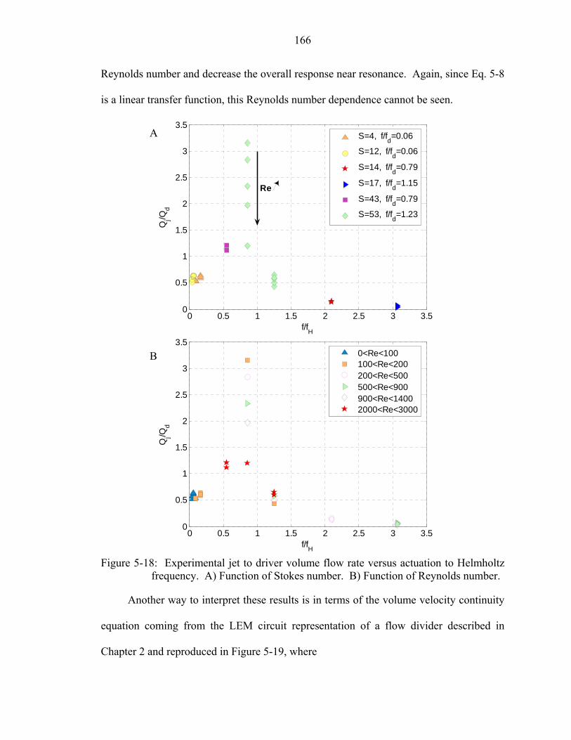
166

Reynolds number and decrease the overall response near resonance. Again, since Eq. 5-8

is a linear transfer function, this Reynolds number dependence cannot be seen.

0 0.5 1 1.5 2 2.5 3 3.50

0.5

1

1.5

2

2.5

3

3.5

f/fH

Qj/Q

d

S=4, f/fd=0.06

S=12, f/fd=0.06

S=14, f/fd=0.79

S=17, f/fd=1.15

S=43, f/fd=0.79

S=53, f/fd=1.23

Re

0 0.5 1 1.5 2 2.5 3 3.50

0.5

1

1.5

2

2.5

3

3.5

f/fH

Qj/Q

d

0<Re<100100<Re<200200<Re<500500<Re<900900<Re<14002000<Re<3000

Figure 5-18: Experimental jet to driver volume flow rate versus actuation to Helmholtz

frequency. A) Function of Stokes number. B) Function of Reynolds number.

Another way to interpret these results is in terms of the volume velocity continuity

equation coming from the LEM circuit representation of a flow divider described in

Chapter 2 and reproduced in Figure 5-19, where

A

B

167

d c jQ Q Q= + , (5-10)

the driver volume velocity being split into the cavity and the orifice branches. Recall that

the Q’s are represented via phasors as complex variables. In view of the above results,

the role of the cavity in this flow divider depends on the value of the cavity impedance

that, as shown above, is related to the Helmholtz frequency. In the limit when the cavity

acoustic impedance aCC tends to zero or for 1Hf f , the impedance 1aC aCZ j Cω=

takes high values and then discourages the flow from going into its branch, which

therefore minimizes the cavity volume velocity cQ since aC c cZ P Q= ∆ . This is the case

when the cavity can be assumed to be incompressible and yields j dQ Q∼ , as seen in the

previous figures. However when the cavity acoustic impedance aCZ takes finite values,

some non-negligible flow enters the cavity branch in Figure 5-19, and in this case where

the cavity is clearly compressible two different scenarios can take place, whether the

actuator is driven near cavity resonance or not. At resonance, the reactance of the

complex impedance in the loop formed with the cavity and the orifice branches is

identically zero and the flow is purely resistive. This case then allows jQ to be greater

than dQ via an acoustic lever arm. At frequencies away from resonance –and/or for

really large cavities- the acoustic impedance of the cavity goes to zero, thus letting the

cavity volume velocity cQ be non-negligible when compared to the other Q’s, thus

yielding a small output flow rate jQ compared to the input dQ . Further consideration on

this matter will be to experimentally compute the cavity volume flow rate. But this is a

non-trivial problem because of the inherent complex nature of the quantity to measure,

and is the subject of future work.

168

ZaD

Z aC

Qc

Qj

∆Pc Z aO

Qd1:φa

PVac

-

+

+

-

+

-

+

-

Figure 5-19: Current divider representation of a piezoelectric-driven ZNMF actuator.

Similarly, another important aspect of this flow divider representation is in the

conservation of power through the different branches of the circuit in Figure 5-19. Power

is defined as the multiplication of an “effort” variable and a “flow” variable. Practically,

it is rather difficult to experimentally estimate the power delivered to the driver, and

especially in the cavity. Nonetheless, the lumped element model should provide

reasonable estimates of the power, and it is shown in Figure 5-20, where again Case 1

from Gallas et al. (2003a) has been used for illustration purposes. In LEM, the governing

equations are written in conjugate power variable form by assuming sinusoidal steady

state operating conditions. Ideally, the piezoelectric diaphragm actuator driver is

modeled as a lossless transformer, which has an input power defined by

d dPw Q P= ⋅ , (5-11)

where P is related to the piezoelectric diaphragm via the two-port element model by

a acP Vφ= ⋅ . (5-12)

The power in the cavity branch is given by

c c cPw Q P= ⋅∆ , (5-13)

and at the orifice exit the power takes the form

j j cPw Q P= ⋅∆ . (5-14)

169

For the power to be conserved in the circuit, the following identity should hold at

any frequency,

j c dPw Pw Pw+ = , (5-15)

and this is plotted in Figure 5-20 where the real and imaginary part of the power is shown

as a function of frequency, taking the parameters from Case 1 (Gallas et al. 2003a).

0 500 1000 1500 2000 2500-0.4

-0.2

0

0.2

0.4

Rea

l

[Pwj + Pwc] - Pwd

0 500 1000 1500 2000 2500-0.4

-0.2

0

0.2

0.4

Imag

inar

y

Frequency (Hz)

fH fd

Figure 5-20: Frequency response of the power conservation in a ZNMF actuator from the

lumped element model circuit representation for Case 1 (Gallas et al. 2003a).

Note that the power is in fact conserved at all frequencies, especially at cavity

resonance when Hf f= . However, at the mechanical resonance, df f= , a jump is

observed which is primarily due to the fact that the piezoelectric diaphragm is modeled as

a lossless transformer that is valid only up to its natural frequency, and beyond this

frequency, the main assumption of LEM fails.

To summarize this chapter, it has been found that the cavity plays an important role

in the actuator response, in terms of geometric parameters and operating frequency.

More particularly, it was found that the pressure inside the cavity may not be equal to the

LEM validity

limit

170

pressure across the orifice, as the LEM assumes it, at least quantitatively in terms of

amplitude. Therefore, care must be taken when using the experimental cavity pressure.

Next, the linear dimensionless transfer function developed from LEM has been

experimentally validated and can be used as a starting guess in a design tool. It is shown

that the cavity can either have a passive role by not affecting the device output, or can

greatly enhance the actuator performance. This is a function of the driver-to-Helmholtz

frequency as well as the Stokes and Reynolds numbers, and for piezoelectric-driven

devices the diaphragm frequency may have a non-negligible impact when df is close to

Hf . More interestingly, large output can be expected ( )j dQ Q at the cavity resonance

but only at low forcing level, the nonlinear orifice resistance tending then to decrease the

output as the input amplitude increases. This says that the optimal response is not simply

given by just maximizing the actuator input. A tradeoff between the cavity design and

actuation amplitude must be made, depending on the desired output to be achieved.

Notice also that this analysis has been made for a piezoelectric-diaphragm driver.

Obviously, using an electromagnetic driver will remove the dimensionless frequency

df f , but the above results still hold and Eq. 5-8 can still be applied since the driver

dynamics are confined in the LHS. Nevertheless, the major impact of this analysis is that

by operating near Hf , the device produces greater output flow rates than the driver due to

the acoustic resonance. An added benefit is that the driver is not operated at mechanical

resonance where the device may have less tolerance to failure.

171

CHAPTER 6

REDUCED-ORDER MODEL OF ISOLATED ZNMF ACTUATOR

In this chapter, the lumped element model of an isolated ZNMF actuator presented

in Chapter 2 is refined based on an investigation of the orifice flow physics. More

precisely, the orifice impedance model is improved to account for geometric and flow

parameter dependence. This refined model stems from a control volume analysis of the

unsteady orifice flow. The results from the experimental setup presented in Chapter 3,

along with the discussion on the orifice and cavity flow physics given in Chapter 4 and

Chapter 5, are used to construct a scaling law of the pressure loss across the orifice,

which is found to be essentially a function of the product of the Strouhal number and the

orifice aspect ratio h/d. This improved lumped element model is then compared along

with the existing previous version (Gallas et al. 2003a) to some experimental test cases.

Orifice Pressure Drop

In the existing lumped element model of an isolated ZNMF actuator presented in

Chapter 2, the major limitation is found in the expression of the nonlinear acoustic orifice

resistance that is directly related to the loss coefficient dK such that,

, 2

0.5 d jaO nl

n

K QR

Sρ

= . (6-1)

A primary goal of this effort is to provide a physical understanding of the orifice flow

behavior, along with a more accurate expression for the coefficient dK in terms of

dimensionless geometric and flow parameters, i.e., in terms of the orifice aspect ratio h/d,

Reynolds number Re, and Strouhal number St. Note that in the existing version of the

172

lumped element model, the coefficient dK is set to unity (McCormick 2000; Gallas et al.

2003a).

In this section, a control volume analysis of the unsteady pressure-driven

oscillatory pipe flow is presented. Figure 6-1 shows a schematic of the control volume

with the coordinate definitions. The governing equations are first derived to obtain an

expression of the pressure drop coefficient across the orifice. Then, the analytical results

are validated via available numerical simulations, which are also used to examine the

relative importance of each term in the governing equation for the orifice pressure drop.

h

boundary layer

δ

potential core fully developed flow

y/h = 0y/h = -1

y

x

ambientregion

cavity

Figure 6-1: Control volume for an unsteady laminar incompressible flow in a circular

orifice, from y/h = -1 to y/h = 0.

Control Volume Analysis

Assuming an unsteady, incompressible, laminar flow and a nondeformable control

volume, as shown in Figure 6-1, the continuity equation becomes

0CV CS CS

d V dA V dAt

ρ ρ∂= ∀+ ⋅ = ⋅∂ ∫ ∫ ∫ , (6-2)

173

or simply inlet exitQ Q= . Since the y location of the outflow boundary is arbitrary, it

directly follows that ( )Q Q y≠ or ( )Q Q t= . Similarly, the y-momentum equation

becomes

yCV CS

F vd v V dAt

ρ ρ∂= ∀+ ⋅∂∑ ∫ ∫ , (6-3)

or, for an axisymmetric orifice,

( ) ( )00

22

y

y n FD FDCV CS

dp p S y dy vd v V dAt

τ τ τ π ρ ρ∂⎛ ⎞− − + − = ∀+ ⋅⎡ ⎤ ⎜ ⎟⎣ ⎦ ∂⎝ ⎠∫ ∫ ∫ , (6-4)

where the subscript ‘FD’ signifies ‘fully developed,’ τ is the wall shear stress, and

( )22nS dπ= is the circular orifice area. Since density is assumed to be constant, the

volume integral can be expressed as follows

( ) ( ) ( )2 2

2 20 0

0 0 0 0

2 2 2 22 2

d dy y

y n FD FD y

Q const

d dp p S y dy y v xdx dy v v xdxt

π τ τ π τ ρ π π

=

⎡ ⎤⎢ ⎥∂

− − − − = ⎢ + − ⎥⎡ ⎤⎣ ⎦ ∂⎢ ⎥⎢ ⎥⎣ ⎦

∫ ∫ ∫ ∫ . (6-5)

Since the volume flow rate is independent of the location y inside the orifice, ( )Q Q y≠ ,

( ) ( ) ( )2

2 20 0

0 0

2 2 22 2

dy

y n FD FD yd d Qp p S y dy y y u u xdx

tπ τ τ π τ ρ π

⎡ ⎤∂− − − − = + −⎡ ⎤ ⎢ ⎥⎣ ⎦ ∂⎢ ⎥⎣ ⎦

∫ ∫ . (6-6)

Then, assuming that the jet volume flow rate is sinusoidal, ( )sinjQ Q tω= , and using

again the time- and spatial- averaged exit velocity during the expulsion stroke jV as the

characteristic velocity, i.e.,

174

( )2

0 0 0

1 12 sin

2 2 2 .

d

j y jn n

Q

j jj

n n

V v xdxdt Q t dtS S

Q QV

S S

π ω π ωω ωπ ωπ π

ωπ ω π π

= =

= = =

∫ ∫ ∫ (6-7)

Next, the integral momentum equation can be written in nondimensional form as

( ) ( ) ( )2 22 1

0 02 2 22

0 0

42 cos 4

1 2 2 2 20.52

y dy yFD FD

jj j jj

p p v vy y x xd y t dd d d dVV V VV

τ τ τ ωπ ωρ ρρ

⎛ ⎞− −− ⎛ ⎞ ⎛ ⎞⎜ ⎟− − = +⎜ ⎟ ⎜ ⎟⎜ ⎟⎛ ⎞ ⎝ ⎠ ⎝ ⎠⎝ ⎠⎜ ⎟⎝ ⎠

∫ ∫ .(6-8)

By using the definition of the Strouhal number jSt d Vω= , and the skin friction

coefficient 2

0.5f jC Vτ ρ= , and defining the normalized pressure drop across the orifice

by

02

0.5y

p

j

p pc

Vρ

−∆ = , (6-9)

Eq. 6-8 can then be rewritten as

( ) ( )2 21

0, , 2

0 0

44 cos 42 2

y dy

p f f FD f FD

jII IIII

IV

v vy y y x xc C C d C St t dd d d d dV

π ω⎛ ⎞− ⎛ ⎞⎛ ⎞ ⎜ ⎟∆ = − + + + ⎜ ⎟⎜ ⎟ ⎜ ⎟⎝ ⎠ ⎝ ⎠⎝ ⎠

∫ ∫ .(6-10)

Eq. 6-10 shows that the pressure drop across the orifice is comprised of four terms:

I = excess shear contribution to the pressure drop II = fully-developed shear contribution III = unsteady inertia term (= 0 if flow is steady) IV = nonlinear unsteady pressure drop to accelerate the flow (convective term) Notice that the first two terms (I and II) can be recombined to yield the total skin friction

coefficient integral, ( )0

4y d

fC d y d∫ , in the pressure drop expression.

175

It should be pointed out that this analysis in derived for an isentropic flow, and that

since only the continuity and momentum equations are used, no assumptions are taken for

the heat transfer. From the energy equation, a simple scaling analysis for the pipe flow

(see end of Appendix C for details) shows that the viscous and thermal boundary layer

are of the same order of magnitude assuming a Prandtl number (ratio of viscous to

thermal diffusivity) of unity for air. However, since no significant heat source is present,

the thermal effect are neglected in this analysis. Notice that Choudhari et al. (1999)

performed a theoretical analysis (confirmed with numerical simulations) on the influence

of the viscothermal effect on flow through the orifice of Helmholtz resonators. They

showed that the thermal effect can be neglected for such flows.

Next, before examining the physics behind the expression for the orifice pressure

drop, one can examine each term in Eq. 6-10 from a numerical simulation to validate this

theoretical analysis and evaluate their relative importance.

Validation through Numerical Results

Once again, the 2D numerical simulations from the George Washington University

described in Appendix F are used to evaluate the analytical expression for the orifice

pressure drop derived above. Three test cases are employed and are referred to as Case 1

(S = 25, St = 2.38, h/d = 1, no jet is formed), Case 2 (S = 25, St = 2.38, h/d = 2, no jet is

formed), and Case 3 (S = 10, St = 0.38, h/d = 0.68, a jet is formed) in the test matrix

shown in Table 2-3. Figure 6-2 shows the variations during one cycle of each of the

terms in Eq. 6-10, for Case 1, Case 2, and Case 3 (Figure 6-2A, Figure 6-2B, and Figure

6-2C, respectively). Actually, the terms I and II in Eq. 6-10 have been recombined

together to remove the explicit fully-developed part and to yield only the total wall shear

stress contribution, since the fully-developed region may not be well defined in these test

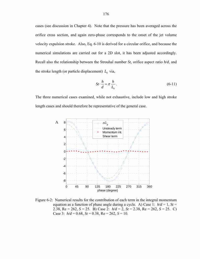
176

cases (see discussion in Chapter 4). Note that the pressure has been averaged across the

orifice cross section, and again zero-phase corresponds to the onset of the jet volume

velocity expulsion stroke. Also, Eq. 6-10 is derived for a circular orifice, and because the

numerical simulations are carried out for a 2D slot, it has been adjusted accordingly.

Recall also the relationship between the Strouhal number St, orifice aspect ratio h/d, and

the stroke length (or particle displacement) 0L via,

0

h hStd L

π⋅ = . (6-11)

The three numerical cases examined, while not exhaustive, include low and high stroke

length cases and should therefore be representative of the general case.

0 45 90 135 180 225 270 315 360

-8

-6

-4

-2

0

2

4

6

8

phase (degree)

∆Cp

Unsteady termMomentum int.Shear term

Figure 6-2: Numerical results for the contribution of each term in the integral momentum equation as a function of phase angle during a cycle. A) Case 1: h/d = 1, St = 2.38, Re = 262, S = 25. B) Case 2: h/d = 2, St = 2.38, Re = 262, S = 25. C) Case 3: h/d = 0.68, St = 0.38, Re = 262, S = 10.

A

177

0 45 90 135 180 225 270 315 360

-15

-10

-5

0

5

10

15

phase (degree)

∆Cp


0 45 90 135 180 225 270 315 360-1

-0.5

0

0.5

1

1.5

phase (degree)

∆Cp



Clearly, it can be seen that the unsteady inertia term – that is directly proportional

to the Strouhal number - is by far the most important contribution in the pressure drop in

the orifice, which is not surprising since the two first cases have a large Strouhal number.

The momentum integral (or convective) and friction coefficient integral terms seem quite

small but actually should not be completely neglected since they contribute in the balance

B

C

178

of the pressure drop, especially for the low Strouhal number Case 3. Notice also how the

pressure drop is shifted by almost 90o (referenced to the volume velocity) which is

primarily due to the unsteady term, but also by the shear stress contribution, the

momentum integral term being in phase with the jet volume flow rate. However, it

should be noted that the results for Case 3 (Re = 262, S = 10, St = 0.38, h/d = 0.68), even

though shown here in Figure 6-2C, should be regarded with caution as some non-

negligible residuals may be present in the computed pressure drop that may be due to

grid/time resolution for extracting the shear stress component and velocity momentum

integral (private communication with Dr. Mittal, 2005). Nonetheless, the results for the

orifice pressure drop magnitude are still used, as seen later.

0 90 180 270 360

0 90 180 270 360

Vex it

Ventrance

Figure 6-3: Definition of the approximation of the orifice entrance velocity from the orifice exit velocity.

Next, the goal is to extend this analysis to practical experimental results. However,

there are no such results available for the velocity profiles at the orifice inlet adjacent to

the cavity or for the friction coefficient along the orifice wall. What are known are the

, ,

, ,

ex inlet in exit

in inlet ex exit

V V

V V

⎧ −⎪⎨

−⎪⎩

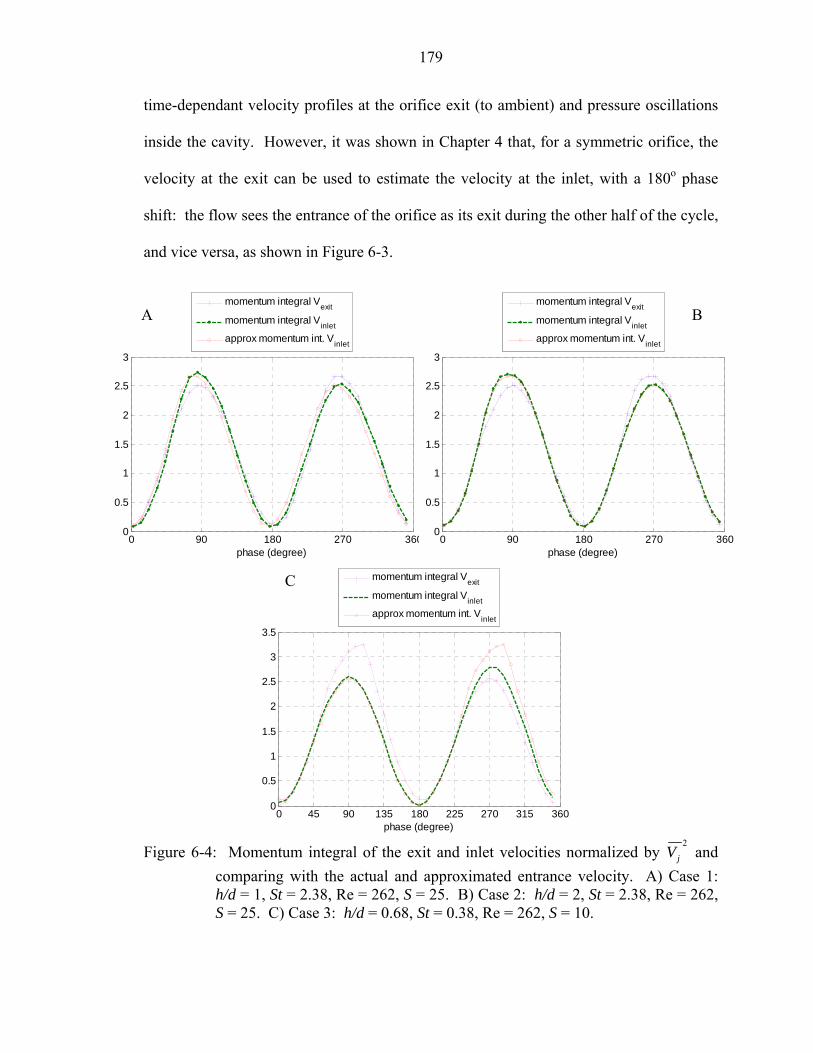
179

time-dependant velocity profiles at the orifice exit (to ambient) and pressure oscillations

inside the cavity. However, it was shown in Chapter 4 that, for a symmetric orifice, the

velocity at the exit can be used to estimate the velocity at the inlet, with a 180o phase

shift: the flow sees the entrance of the orifice as its exit during the other half of the cycle,

and vice versa, as shown in Figure 6-3.

0 45 90 135 180 225 270 315 3600

0.5

1

1.5

2

2.5

3

3.5

phase (degree)

momentum integral Vexit

momentum integral Vinlet

approx momentum int. Vinlet

Figure 6-4: Momentum integral of the exit and inlet velocities normalized by

2

jV and comparing with the actual and approximated entrance velocity. A) Case 1: h/d = 1, St = 2.38, Re = 262, S = 25. B) Case 2: h/d = 2, St = 2.38, Re = 262, S = 25. C) Case 3: h/d = 0.68, St = 0.38, Re = 262, S = 10.

0 90 180 270 3600

0.5

1

1.5

2

2.5

3

phase (degree)




0 90 180 270 3600

0.5

1

1.5

2

2.5

3

phase (degree)




A B

C

180

This approximation for the entrance velocity is further verified via Case 1, Case 2,

and Case 3. The normalized momentum integral of the exit and inlet velocities, defined

by 21 021 2

j

v xddV−

⎛ ⎞⎜ ⎟⎝ ⎠

∫ and 2

1

21 2y h

j

v xddV

=

−

⎛ ⎞⎜ ⎟⎝ ⎠

∫ are plotted in Figure 6-4A and Figure 6-4B, and

Figure 6-4C, respectively for Case 1, Case 2, and Case 3, during one cycle along with the

approximated momentum integral of the inlet velocity. As can be seen, the result for the

approximated inlet velocity is in fair agreement with the actual entrance velocity,

although for the large stroke length case (Case 3) the inlet velocity is slightly

overpredicted by the approximated one but only during the ingestion stroke. It should be

emphasized that this is only valid for a symmetric orifice.

Finally, the sum of the source terms in Eq. 6-10 that balance the pressure drop pc∆

are plotted as a function of time for the first two numerical test cases (as noted above,

Case 3 is not shown here). Results from using both the actual and approximate entrance

velocity are also shown in Figure 6-5. Clearly, the CFD results confirm the validity of

Eq. 6-10. Therefore, Eq. 6-10 can be used with confidence to compute the pressure drop

across the orifice, and the orifice entrance velocity can also be computed from the orifice

exit velocity in the experimental results, and the corresponding time- and spatial-

averaged velocity can be defined as

, ,

, ,

ex inlet in exit

in inlet ex exit

V V

V V

⎧ −⎪⎨

−⎪⎩. (6-12)

181

0 90 180 270 360-10

-8

-6

-4

-2

0

2

4

6

8

10

phase (degree)

∆cp

Tunsteady + actual(Tmomentum) + Tshear

Tunsteady + approx(Tmomentum) + Tshear

0 90 180 270 360-20

-15

-10

-5

0

5

10

15

20

phase (degree)

∆cp

Tunsteady + actual(Tmomentum) + Tshear

Tunsteady + approx(Tmomentum) + Tshear

Figure 6-5: Total momentum integral equation during one cycle, showing the results

using the actual and approximated entrance velocity. A) Case 1: h/d = 1, St = 2.38, Re = 262, S = 25. B) Case 2: h/d = 2, St = 2.38, Re = 262, S = 25.

Discussion: Orifice Flow Physics

Now that Eq. 6-10 has been validated via numerical simulations, it is worthwhile to

examine the physics behind each term that compose Eq. 6-10, as discussed below.

A

B

182

I = excess shear contribution to the pressure drop

This is a linear contribution to the pressure drop. It corresponds to the excess shear

needed to reach a fully developed state (in which the time-dependent velocity profile is

invariant along the length of the orifice). In particular, it corresponds to the viscous

effect in a starting orifice flow and is expected to have both dissipative (resistance) and

inertial (mass) components since it will affect the magnitude and phase of the pressure

drop. This is in accordance with the discussion provided on the velocity profiles shown

in Chapter 4 in Figure 4-2, Figure 4-3, and Figure 4-4 for Case 1, Case 2, and

Case 3 , respectively. However, as seen from the numerical results (Figure 6-2), this term

appears to be negligible for the low and large Strouhal number cases examined. It is

therefore neglected in the rest of this analysis.

II = fully developed shear contribution to the pressure drop

This is again a linear contribution to the pressure drop. In fact, the friction

coefficient term comes from viscous effects at the orifice walls that are linear by nature.

In the case of a fully developed, steady orifice flow, the corresponding pressure loss can

be written as

2

,142f FD j

hP C Vd

ρ∆ = , (6-13)

or, since ( ), 16 Re 16jf FD jV

C V d ν= = and j jV V= for a steady pipe flow (White 1991),

it directly follows that

2

2

324 16 12

jj

j

hVhP Vd dV d

µρ

ν∆ = = , (6-14)

which can be recast in terms of an acoustic impedance

183

( ) ,44

128 82

aO aO linj

P h hZ RQ d d

µ µπ π

∆= = = = . (6-15)

This is exactly the linear acoustic resistance ,aO linR of the orifice due to viscous

effect derived previously in Chapter 2. Hence, the shear term II in Eq. 6-10 corresponds

to the viscous linear resistance in the existing lumped element model. As a validation,

the numerical data from Case 1 and Case 2 are again used. In Figure 6-6A and Figure

6-6B the total shear stress contribution (terms I and II) from the numerical data for Case 1

and Case 2, respectively, are compared with the corresponding acoustic linear resistance

,aO linR that actually only models term II. Clearly, the magnitude of the fully developed

contribution (term II) is dominant, while the main effect of the excess shear is believed to

add a small phase lag in the signal. This result provides confidence in the assumption of

neglecting the excess shear contribution, i.e. term I.

Figure 6-6: Numerical results of the total shear stress term versus corresponding lumped

linear resistance during one cycle. A) Case 1: h/d = 1, St = 2.38, Re = 262, S = 25. B) Case 2: h/d = 2, St = 2.38, Re = 262, S = 25.

0 45 90 135 180 225 270 315 360-1.5

-1

-0.5

0

0.5

1

1.5

phase (degree)

Total shear term (I + II)RaO,linear <=> Shearfully developed (II)

0 45 90 135 180 225 270 315 360

-0.5

-0.4

-0.3

-0.2

-0.1

0

0.1

0.2

0.3

0.4

0.5

phase (degree)

Total shear term (I + II)RaO,linear <=> Shearfully developed (II)

B A

184

III = unsteady inertia term

This is again a linear contribution to the orifice pressure drop, with a 90o phase

shift referenced to the volume flow rate (or velocity). In a similar manner as above, the

unsteady term contribution can be rewritten such that

21

2 jhP St Vd

π ρ∆ = , (6-16)

or in terms of an acoustic impedance,

212 3 4 3

4 3 42

jj

aO aNj n n

j n

h d Vd VP h hZ M

Q S SV S

ωπ ρωρ ρω ωπ

∆= = = = = , (6-17)

where aNM is the linear acoustic mass of the orifice associated with the fully developed

pipe flow. Therefore, the unsteady inertia term is equivalent to a mass (or inertia) in the

orifice. Notice that Eq. 6-17 is derived for a circular orifice and that in the case of a 2D

slot the multiplicative constant is equal to 5/6 instead of 3/4.

Figure 6-7: Numerical results of the unsteady term versus corresponding lumped linear

reactance during one cycle. A) Case 1: h/d = 1, St = 2.38, Re = 262, S = 25. B) Case 2: h/d = 2, St = 2.38, Re = 262, S = 25.

0 45 90 135 180 225 270 315 360-15

-10

-5

0

5

10

15

phase (degree)

(∆cp)Unsteady term

ω.5/6.MaN

0 45 90 135 180 225 270 315 360-8

-6

-4

-2

0

2

4

6

8

phase (degree)

(∆cp)Unsteady term

ω.5/6.MaN

B A

185

Again, the CFD data are compared with the corresponding linear lumped parameter

aNM , as shown in Figure 6-7A and Figure 6-7B for Case 1 and Case 2, respectively.

This term along with the skin friction integral (term I, which is also frequency dependant

when the flow is not steady) are the sources of the reactance term in the linear acoustic

total orifice impedance model aO aO aOZ R j Mω= + .

IV = momentum integral term

The momentum integral that comes from the convective term is the nonlinear term

that is the source of the distortion in the orifice pressure loss signal. As a simple

example, if the flow is steady and if the location y is chosen such that the flow is fully

developed, then the velocity is given by

( )( ) ( )

2 2

2 22 1 12 2y j j

x xv x V Vd d

π⎛ ⎞ ⎛ ⎞

= − = −⎜ ⎟ ⎜ ⎟⎜ ⎟ ⎜ ⎟⎝ ⎠ ⎝ ⎠

, (6-18)

and, by assuming a uniform velocity profile at the orifice inlet, the last integral (term IV

in Eq. 6-10) would be simply 2/3, exactly that found for the case of steady flow in the

inlet of ducts derived in White (1991, p. 291). However, in the general case, this term is

both resistive and reactive i.e., it has a magnitude and a phase component, as shown from

the numerical results of Case 1 and Case 2 in Figure 6-8A and Figure 6-8B, respectively.

The magnitude of this nonlinear term is clearly non-negligible at low St h d⋅ (or high

dimensionless stroke length 0L h ) as seen in Figure 6-2. Also, as shown in Figure 6-8,

the momentum integral clearly exhibits a 3ω component. This suggests that the

nonlinear term IV cannot be only modeled by a nonlinear resistor, but should also have a

reactance component.

186

In this regard, one can use a zero-memory “square-law with sign” model in the

momentum integral expression (Bendat 1998), which is defined by

Y X X= , (6-19)

where the output Y would correspond to the output pressure drop and the input X is the

spatial averaged velocity at any location y inside the orifice. It can be easily shown (see

Bendat (1998) who performed a similar derivation but for an input white noise) that by

assuming the input X as a sine wave given by

( ) ( )sinX t A tω φ= + , (6-20)

where A is the magnitude and the phase ( π φ π− ≤ ≤ ) is uniformly distributed, and by

minimizing the mean square estimate, then this square-law with sign model can be

successfully approximated by a cubic polynomial Y of the form

316 3215 15

AY X X X XAπ π

= ≅ + . (6-21)

Notice that the ratio between the two polynomial coefficients is equal to 22 A , which is

over the inverse of the power in the input sine wave. Substituting Eq. 6-20 in Eq. 6-21,

the output of the zero-memory square-law with sign nonlinear model takes the form

( ) ( ) ( )28 1sin sin 3 3

3 5AY t t tω φ ω φπ

⎡ ⎤= + − +⎢ ⎥⎣ ⎦. (6-22)

The square law with sign produces a cubic nonlinearity. The nonlinear system

redistributes energy to the fundamental (ω) and to the 2nd harmonic (3ω). Notice also the

relative magnitude between the two contributions in Eq. 6-22 such that it looks like the

nonlinear contribution is small while the linear contribution is large. This principal

feature of the model can clearly be seen in the numerical results shown in Figure 6-8.

187

How to correlate this square-law with sign model with the momentum integral (term IV in

Eq. 6-10) is investigated in the next section.

Figure 6-8: Numerical results of the normalized terms in the integral momentum

equation as a function of phase angle during a cycle. A) Case 1: h/d = 1, St = 2.38, Re = 262, S = 25. B) Case 2: h/d = 2, St = 2.38, Re = 262, S = 25. Each term has been normalized by its respective magnitude.

In summary, a physical explanation has been given of each of the term that

composes the equation of the orifice pressure drop given by Eq. 6-10. Each term was

related to its lumped element counterpart. It was found that the excess shear contribution

from the starting flow (term I) can be neglected in comparison to the magnitude of the

other terms, the fully developed shear stress component (term II) is equivalent to the

linear acoustic resistance from LEM, and the unsteady inertia term (term III) corresponds

to the acoustic linear orifice reactance. Finally, the momentum integral (term IV) is the

only nonlinear contribution to the pressure drop and can be represented by a nonlinear

system having both a resistive ( ),aO nlR and a reactive ( ),aO nlM part. Therefore, if one is

able to find a correlation for this nonlinear term (term IV) as a function of the governing

dimensionless parameters, then it can be implemented into the existing low-order lumped

0 45 90 135 180 225 270 315 360-1

-0.8

-0.6

-0.4

-0.2

0

0.2

0.4

0.6

0.8

1

phase (degree)

∆Cp

Unsteady term (III)Momentum int. (IV)Shear term (I+II)

0 45 90 135 180 225 270 315 360-1

-0.8

-0.6

-0.4

-0.2

0

0.2

0.4

0.6

0.8

1

phase (degree)

∆Cp

Unsteady term (III)Momentum int. (IV)Shear term (I+II)

B A

188

model. These findings are shown schematically in Figure 6-9, where a physical parallel

is provided between each of the terms in the acoustic orifice impedance of a ZNMF

actuator and the control volume analysis described above.

Figure 6-9: Comparison between lumped elements from the orifice impedance and

analytical terms from the control volume analysis.

Development of Approximate Scaling Laws

Experimental results

Now that an analytical expression of the pressure drop across the orifice has been

derived and validated, the experimental data presented in Chapter 3 and used throughout

this dissertation are used to develop scaling laws of the orifice pressure drop coefficient,

LEM

( ) ( ), , , ,aO aO linear aO nonlinear aO linear aO nonlinearj

PZ R R j M MQ

ω ∆= + + + =

Con

trol v

olum

e an

alys

is

( ) ( )2 2

20

,

10

,0

c 4o42

4 s2

y d

f f F Fpy

j

D f Dy v v x xdC

d d dyC C d y Sc t

d Vt

dπ ω∆ = + + +⎛ ⎞− ⎜ ⎟

⎝ ⎠

⎛ ⎞− ⎛ ⎞⎜ ⎟ ⎜ ⎟⎜ ⎟ ⎝ ⎠⎝ ⎠∫ ∫

aNRfaCR0

,aO nlR faCM0

aNM

,

linear resistance due to starting developing viscous flow (neglected)

linear resistance due to fully-developed viscous flow nonlinear resistance due to velocity momentum react

faC

aN

aO nl

aN

R

RR

Mω

⇒

⇒⇒

⇒

,

ance due to flow unsteadinessreactance due to starting developing viscous flow (neglected)

nonlinear reactance due to velocity momentumfaC

aO nl

M

M

ω

ω

⎧⎪⎪⎪⎪⎨⎪⎪ ⇒⎪⎪ ⇒⎩

,aO nlM

189

to improve the existing lumped element model. In Chapter 4, the experimentally

determined orifice pressure loss coefficient has already been plotted versus the Strouhal

number as well and the nondimensional stroke length 0St h d h Lπ= . However, large

scatter in the pressure data were noted, since it was assumed that the pressure inside the

cavity is equivalent to the pressure drop across the orifice. This is not always a valid

assumption, as discussed in the first part of Chapter 5. Therefore, the RHS of Eq. 6-10 is

now used explicitly to compute the orifice pressure drop pc∆ . Notice however that the

shear stress contribution is neglected in this experimentally-based investigation, simply

because no such information is available and also since, as discussed above, the CFD

results suggest that this term is indeed negligible. Likewise, as validated in the previous

section, the entrance velocity is approximated by the exit velocity via Eq. 6-12 to

compute the velocity momentum integral (term IV in Eq. 6-10).

Figure 6-10 shows the experimental results of the total orifice pressure drop

coefficient for different Stokes number and as a function of St h d⋅ . The pc∆ is

computed from the control volume analysis (using the RHS of Eq. 6-10 less the shear

term). However, the pc∆ measured from the cavity pressure data using Microphone 1 or

Microphone 2 is also shown only for illustration purposes. In addition to the

experimental results, the results for the numerical simulations used above are included.

The experimental results using the theoretical control volume analysis show good

collapse of the data over the whole range of interest. This is especially true even at high

St h d⋅ (or low dimensional stroke length by recalling that 0St h d h Lπ⋅ = ⋅ ) where the

orifice pressure drop linearly increases with St h d⋅ . This is in accordance with the fact

190

that the unsteady term in Eq. 6-10 is a function of St h d⋅ and was shown to be the

dominant term. However, at lower values ( )1St h d⋅ < , the collapse in the data is less

pronounced since for such low Strouhal numbers the nonlinear term becomes significant

due to jet formation, as confirmed from the CFD data and shown previously in Gallas et

al. (2004). In this scenario at low St h d⋅ , the orifice flow may be seen as quasi-steady

and/or as a starting flow due to the large stroke length; hence the pressure drop should

asymptote to the solution of steady pipe flow, which is mainly a function of geometry and

Reynolds number. Notice also that the case of low St h d⋅ may also be due to a very

thin orifice design, similar to a perforate, for which the orifice flow is always in a

developing state.

On the other hand, the scatter in the data using the experimental cavity pressure is

made evident when joining the corresponding data from Mic 1 to Mic 2 to estimate the

uncertainty in the pressure data. Although the orifice pressure drop is overestimated for

certain experimental data cases when using the cavity pressure information, given the

large uncertainty in the pressure drop data, the overall trend is well-defined over the

intermediate-to-high range of St h d⋅ , while the lower range shows an asymptotic

behavior to a constant value. In any case, the two distinct regions are well defined. At

low dimensionless stroke length, the flow is clearly unsteady, while for high

dimensionless stroke length the flow is quasi-steady, as delimited by the dotted line in

Figure 6-10, which corresponds to 0.62St h d⋅ , or 0 5L h .

191

10-2

10-1

100

101

102

10-1

100

101

102

103

St.h/d = π .h/L0

∆c p= ∆

P/(0

.5ρV

j2 )

S=4S=10S=12S=14S=17S=25S=43S=53

∆p using Control Volume∆p using Mic 1

∆p using Mic 2

CFD

0.62

Figure 6-10: Experimental results of the orifice pressure drop normalized by the dynamic

pressure based on averaged velocity jV versus St h d⋅ for different Stokes numbers. The pressure drop is computed using either the control volume analysis (terms III and IV) or the experimental cavity pressure (Mic 1 and Mic 2).

Next, each term in Eq. 6-10 - less term I that is neglected - is also plotted versus the

dimensionless stroke length St h d⋅ using the experimental data. Practically, the

nonlinear momentum integral (term IV) is computed from the exit velocity profile and

using the approximation discussed above to compute the orifice entrance velocity (recall

the equivalence with the nonlinear acoustic resistance RaO,nl and mass MaO,nl). The

unsteady inertia component (term III) is directly computed via its definition (equivalent

to the acoustic mass MaN). Then, the fully developed friction coefficient contribution

(term II) is also computed from its definition (recall the equivalence with the linear

acoustic resistance RaN). The experimental results for these three terms are shown in

Figure 6-11.

192

10-1

100

101

102

0

0.5

1

1.5

2

2.5

3

3.5

4

4.5

St.h/d

S=4S=10S=12S=14S=17S=25S=43S=53

Figure 6-11: Experimental results of each term contributing in the orifice pressure drop coefficient vs. St h d⋅ . A) Term II: friction coefficient integral due to fully developed flow. B) Term III: unsteady inertia. C) Term IV: nonlinear momentum integral from convective term.

First of all, the contribution of the friction coefficient integral from the fully

developed pipe flow that corresponds to the linear acoustic resistance in the LEM is

shown in Figure 6-11A. Not surprisingly, it has a rather small effect overall and linearly

increases with St h d⋅ . Note that the data will collapse if one plots it as a function of

( ) Reh d (recall that 2 ReSt S= ). Then, shown in Figure 6-11B, is the contribution of

10-2

10-1

100

101

102

10-1

100

101

102

103

St.h/d

S=4S=10S=12S=14S=17S=25

10-2

10-1

100

101

102

10-3

10-2

10-1

100

101

St.h/d

S=4S=12S=14S=17S=43S=53

A B

Unsteady inertia Fully developed flow friction coefficient integral

C Nonlinear momentum integral

193

the unsteady inertia effects that varies linearly with St h d⋅ , and which is clearly the

dominant feature in the total orifice pressure loss, especially for 0.62St h d⋅ > . Figure

6-11C shows next the variations of the nonlinear momentum integral as a function of the

dimensionless stroke length. It can first be noted that the data seem scattered and that no

obvious trend can be discerned. Notice also that the data oscillate around a value of

unity, which is the assumed value for the nonlinear loss coefficient Kd in the existing

lumped model. Finally, Figure 6-12 shows the relative magnitudes of each term in the

pressure loss equation for the intermediate to low St h d⋅ cases. It confirms that the

nonlinear term is only really significant for low values of 3St h d⋅ < , where above this

value the unsteady inertia term (term III) dominates and takes on a value greater than 10

(see Figure 6-11C), while term IV never exceeds 2 (and is usually less than that).

0 0.5 1 1.5 2 2.5 3 3.5 4 4.50

10

20

30

40

50

60

70

80

90

100

St.h/d

perc

enta

ge (%

)

Fully developed shear (term II)Unsteady inertia (term III)Mometum integral (term IV)

Figure 6-12: Experimental results of the relative magnitude of each term contributing in

the orifice pressure drop coefficient vs. intermediate to low St h d⋅ .

Therefore, based on these experimental results from the control volume analysis,

the next step to be undertaken is to obtain a correlation of the nonlinear term in the

194

pressure drop expression, which is ultimately to be related to the nonlinear coefficient Kd

from the LEM defined in previous chapters. The other terms in Eq. 6-10 are already

defined, as shown in Figure 6-9. Then the scaling law will be implemented in the

existing lumped model from Gallas et al. (2003a) to yield a refined model.

Nonlinear pressure loss correlation

In the previous section, it was shown that the nonlinear part of the pressure loss

coefficient can be successfully approximated by a square-law with sign model, which has

both magnitude and phase information. The experimental results are then used to find a

correlation for the magnitude. However, it is difficult to obtain accurate phase

information at the present time. Since we are primarily interested in the magnitude of the

actuator output, we will concentrate on the nonlinear resistance component. Applications

that require accurate phase information (e.g., feedback flow control models) will

ultimately require this aspect to be addressed.

As shown in Figure 6-11C, there is no such obvious correlation for the magnitude

from the data over the entire range of St h d⋅ . However, as noted earlier, two regions of

operation can be distinguished from each other. A quasi-steady flow for high

dimensionless stroke length ( )0 5L h > and unsteady flow for intermediate to lower

0L h .

In the former case where the nonlinear term IV is important, a different functional

form should be envisaged from known steady pipe flow solutions that usually rely on the

orifice geometry and flow Reynolds number. For instance, when studying flows in the

inlet of ducts, White (1991, p. 291) describes a correlation of the pressure drop in the

entrance of a duct for a laminar steady flow as a function of ( ) Rey d . Also, another

195

common approach employed is from orifice flow meters. There, from pipe theory

(Melling 1973; White 1979), the steady pipe flow dump loss coefficient for a generalized

nozzle is given by

( ) 241d DK Cβ

−

= − , (6-23)

with d Dβ = is the ratio of the exit to the entrance orifice diameter, and where DC is

the discharge coefficient that takes the form

( )0.50.9975 6.53 ReDC β= − (6-24)

for high Reynolds number Re . The problem however resides in the facts that Eq. 6-23 is

based on a beveled-type of orifice, and that it is valid only for high Reynolds number

( )4Re 10> .

Here, a similar approach is used to correlate the quasi-steady cases. This is shown

in Figure 6-13 where the experimentally determined nonlinear loss (∆cp)nonlinear is plotted

against the Reynolds number Re in Figure 6-13A and against ( ) Reh d in Figure 6-13B.

In these plots, the circled data are the ones of interest since they occur at a low St h d⋅

i.e., 0.62St h d⋅ < or 0 5L h > . Note that a distinction has been made on the orifice

aspect ratio h/d (small h/d are in red symbols, intermediate h/d are in green, and large h/d

are in blue). Once again, the 3 numerical test cases have been added to the figures for

completeness. An estimate can then be found for the low St h d⋅ range in terms of

( ) Reh d , as shown by the regression line in Figure 6-13B. The two outliers in Figure

6-13B are Case 60 (S = 4, h/d = 5, Re = 132, St = 0.12) and Case 61 (S = 4, h/d = 5, Re =

157, St = 0.10).

196

101

102

103

104

0

0.5

1

1.5

2

2.5

3

3.5

4

4.5

Re

Kd =

( ∆c p) N

onlin

ear

S=4, h/d=0.94S=4, h/d=5S=10, h/d=0.68S=12, h/d=1.68S=12, h/d=0.35S=14, h/d=5S=17, h/d=5S=25, h/d=1S=25, h/d=2S=43, h/d=0.35S=53, h/d=0.35S=53, h/d=1.68

small h/dintermediate h/d

large h/d

0 0.01 0.02 0.03 0.04 0.05 0.060

0.5

1

1.5

2

2.5

3

3.5

4

4.5

(h/d)/Re

Kd =

( ∆c p) N

onlin

ear

S=4, h/d=0.94S=4, h/d=5S=10, h/d=0.68S=12, h/d=1.68S=12, h/d=0.35S=14, h/d=5S=17, h/d=5S=25, h/d=1S=25, h/d=2S=43, h/d=0.35S=53, h/d=0.35S=53, h/d=1.68

small h/d

intermediate h/d

large h/d

Kd=(1-20(h/d)/Re)/(0.4+300(h/d)/Re)

Figure 6-13: Experimental results for the nonlinear pressure loss coefficient for different Stokes number and orifice aspect ratio. A) Versus Reynolds number Re. B) Versus ( ) Reh d . The circled data correspond to 0 5L h > .

On the other hand, for the case of intermediate to high St h d⋅ , one can find a

crude correlation as a function of St h d⋅ , as shown in Figure 6-14, that should be able to

represent the principal variations in the nonlinear part of the orifice pressure loss. Once

A

B

(∆c p

) non

linea

r (∆

c p) n

onlin

ear

197

again, the 3 numerical test cases have been added to the figure for completeness. The

two outliers in Figure 6-14 are Case 48 (S = 53, h/d = 0.35, Re = 571, St = 4.96) and Case

56 (S = 53, h/d = 1.68, Re = 318, St = 8.79).

10-1

100

101

102

0

0.5

1

1.5

2

2.5

3

3.5

4

4.5

St.h/d

Kd =

( ∆c p) N

onlin

ear

S=4S=10S=12S=14S=17S=25S=43S=53

Kd=0.43+(St.h/d)-1

0.62

Figure 6-14: Nonlinear term of the pressure loss across the orifice as a function of

St h d⋅ from experimental data. The straight line shows a curve fit to the data in the intermediate to high St h d⋅ range.

Therefore, based on these simple regressions performed on the data, a rough

correlation on the amplitude of the nonlinear pressure loss coefficient can be obtained as

a function of St h d⋅ . At low values of St h d⋅ , the nonlinear coefficient varies with

( ) Reh d , while for intermediate to high values, the nonlinear pressure drop coefficient

is a function of St h d⋅ . Thus, the following scaling law of the amplitude of the

dimensionless orifice pressure loss is proposed

(∆c p

) non

linea

r

198

0,

-10

,

1 20Re for 0.62 or 5

0.4 300Re

0.43 for 0.62 or 5

p nl

p nl

h dLhc St

h d d h

Lh hc St Std d h

⎧ ⎛ ⎞− ⎜ ⎟⎪ ⎝ ⎠⎪ ∆ = ⋅ < >⎛ ⎞⎪ + ⎜ ⎟⎨ ⎝ ⎠⎪

⎪ ⎛ ⎞∆ = + ⋅ ⋅ ≥ ≤⎪ ⎜ ⎟⎝ ⎠⎩

. (6-25)

Notice that these scaling laws are not optimal since they do not overlap at 0.62St h d⋅ = .

Although for high St h d⋅ it seems accurate, the functional form for the scaling law for

low St h d⋅ can be greatly refined from an extended available database.

Then, based on this development of a scaling law for the nondimensional pressure

loss inside the orifice of an isolated ZNMF actuator, the next logical step is to implement

it into the existing reduced-order lumped element model. This is described in the

following section.

Refined Lumped Element Model

Implementation

The lumped element model presented in Chapter 2 has been derived from the

hypothesis of fully developed pipe or channel flow. The acoustic impedance of the

orifice, which is the component to be improved, is defined as a complex quantity that has

both a resistance and a reactance term (Gallas et al. 2003a),

, ,aO aO lin aO nl aOZ R R j Mω= + + , (6-26)

where ,aO linR and aOM are, respectively, the linear acoustic resistance and mass (i.e.,

reactance) terms from the exact solution for steady fully-developed pipe flow. The

nonlinear acoustic resistance, ,aO nlR , is defined as

, 2

0.5 d jaO nl

n

K QR

Sρ

= , (6-27)

199

where Kd is the dimensionless orifice loss coefficient that is assumed to be unity

(McCormick 2000) in the existing version of the lumped element model.

From the previous analysis using a control volume, the correspondence between the

lumped elements and the pressure drop terms was shown in Figure 6-9. All terms were

appropriately modeled via lumped elements except for the nonlinear term that is the focus

of this effort and that has both a resistance and a reactance. From the scaling law

developed next, only the magnitude was successfully correlated with the main

nondimensional geometric and flow parameters, not the phase. The magnitude and phase

of the nonlinear term are related to the resistance and mass in the LEM impedance

analogy via the following relationships. Since the acoustic impedance is defined as

aO aO aOj

PZ R j MQ

ω ∆= + = , (6-28)

and that the orifice pressure drop is

20.5

p

j

PcVρ

∆∆ = , (6-29)

then, the correspondence between LEM and the control volume analysis is given by

jaO p

j n

VPZ cQ S

ρπ

⎛ ⎞∆= = ∆⎜ ⎟⎜ ⎟

⎝ ⎠. (6-30)

However, the nonlinear pressure drop from the momentum integral was shown to be

accurately modeled via a square-law with sign model (see Eq. 6-22). So accounting only

for the nonlinear part, Eq. 6-30 becomes

200

( ) ( )

, , , ,

315

nl nl

jaO nl aO nl aO nl p nl

n

j t A j t Anl

VZ R j M c

S

A e eω ω

ρω

π

+∠ +∠

⎛ ⎞= + = ∆⎜ ⎟⎜ ⎟

⎝ ⎠⎧ ⎫= ⋅ −⎨ ⎬⎩ ⎭

(6-31)

where ( ) ,nl j n p nlA V S cρ π= ∆ . Notice also that the relationship between the

dimensionless orifice loss coefficient Kd defined in Eq. 6-27 and the nonlinear part of

pc∆ defined in Eq. 6-29 is such as

2

,2

d p nlK cπ⎛ ⎞= ∆⎜ ⎟⎝ ⎠

. (6-32)

Hence, the parameters introduced in Eq. 6-31 are related to each other via,

( ) ( )2 22

, ,

,

,

cot

nl aO nl aO nl

aO nlnl

aO nl

A R M

MA

R

ω

ω

⎧ = +⎪⎪⎨ ⎛ ⎞∠ =⎪ ⎜ ⎟⎜ ⎟⎪ ⎝ ⎠⎩

. (6-33)

The problem resides in the fact that, even though a scaling law was developed for

the nonlinear magnitude nlA , insufficient information is available to model the nonlinear

phase component nlA∠ . Hence the system of equation Eq. 6-33 cannot be solved for both

,aO nlR and ,aO nlM . Nonetheless, as a first pass, the phase lag from the nonlinear term is

neglected, so that the scaling law developed above in Eq. 6-25 for ,p nlc∆ is directly

implemented into the total orifice acoustic impedance ZaO through the refined nonlinear

acoustic resistance ,aO nlR via Eqs. 6-31 and 6-32.

201

start

input actuatordesign

frequency loopf > flim

compute lumpedparameters:

,, , ,aD aC aO aO linZ Z M R

computenonlinear lumped

parameters:,d aO nl aOK R Z→ →

initial guess

compute jet volume flow rateac a

jaC aD aC aO aO aD

VQZ Z Z Z Z Z

φ=

+ +

end

newguess

Newton-Raphsonalgorithm

compute jet velocityj j nV Q S=

convergencecriterion

F

T

T

F

Figure 6-15: Implementation of the refined LEM technique to compute the jet exit velocity frequency response of an isolated ZNMF actuator.

202

Comparison with Experimental Data

The problem being now closed, the refined lumped element model can now be

implemented and compared to experimental data. Notice that Kd is now a function of the

output flow, so it should be implemented in an iterative converging loop. Also, LEM

provides a frequency response of the actuator output (strictly speaking, it is an impulse

response since the system is nonlinear). The actual sequence to compute the jet exit

velocity using the refined LEM technique is depicted in the flowchart shown in Figure

6-15. The nonlinear terms in the orifice acoustic impedance are computed via a Newton-

Raphson algorithm.

Next, the refined low-order model is implemented and compared with available

frequency response experimental data. The two test cases that were used to validate the

first version of the lumped model in Gallas et al. (2003) are again utilized for

comparison. These two cases are already shown in Chapter 2 (see Figure 2-2), and the

reader is referred to Gallas et al. (2003a) for the details of the experimental setup and

actuator configuration. In Figure 6-16 and Figure 6-17, the impulse response of the jet

exit velocity acquired at the centerline of the orifice is compared with the two lumped

element models: the “previous LEM” corresponds to the model developed in Gallas et al.

(2003a), and the “refined LEM” corresponds to the refined model developed in this

chapter. Each model prediction is applied to Case I and Case II, as shown in Figure

6-16A and Figure 6-17A, respectively. Notice that here the only empirical factor – the

diaphragm damping coefficient Dζ - has been adjusted so that the refined model matches

the peak magnitude at the frequency governed by the diaphragm natural frequency.

203

Before discussing the results, it should be pointed out that the experimental data are

for the centerline velocity ( )CLV t of the ZNMF device. The lumped element model gives

a prediction of the jet volume flow rate amplitude (or spatial-averaged exit velocity

( )jV t ) which is like a “bulk” velocity. And as seen in Chapter 4, there is no simple

relationship between ( )jV t and ( )CLV t (see Figure 4-10) for the test cases considered in

this study. Therefore, in order to represent this uncertainty, the two minima from the

theoretical ratio j CLV V for a fully developed pipe flow, that is already shown in Figure

2-5, are bounding the refined LEM prediction, as seen in Figure 6-16A and Figure 6-17A.

0 500 1000 1500 2000 2500 30000

5

10

15

20

25

30

35

frequency (Hz)

cent

erlin

e ve

loci

ty (m

/s)

exp. dataprevious LEMrefined LEM

bounds in the expectedvalue of V

CL for LEM

Figure 6-16: Comparison between the experimental data and the prediction of the refined

and previous LEM of the impulse response of the jet exit centerline velocity. A) Centerline velocity versus frequency, where the LEM prediction is bounded by the minima of the theoretical ratio j CLV V . B) Jet Reynolds number versus S2. C) Nonlinear pressure loss coefficient versus S2. Actuator design corresponds to Case I from Gallas et al. (2003a).

A

204

0 500 1000 1500 2000 2500 3000 3500 4000 45000

500

1000

1500

2000

2500

3000

3500

4000

S2

Rey

nold

s nu

mbe

r

exp. datarefined LEM

Re based on VCL

Re based on Vj

/ \

0 500 1000 1500 2000 2500 3000 3500 4000 45000

0.2

0.4

0.6

0.8

1

1.2

S2

Kd


Similarly, the Reynolds number based either on CLV for the experimental data or jV

for the LEM prediction is plotted versus the Stokes number squared, as shown in Figure

6-16B and Figure 6-17B. And finally, Figure 6-16C and Figure 6-17C show the

C

B

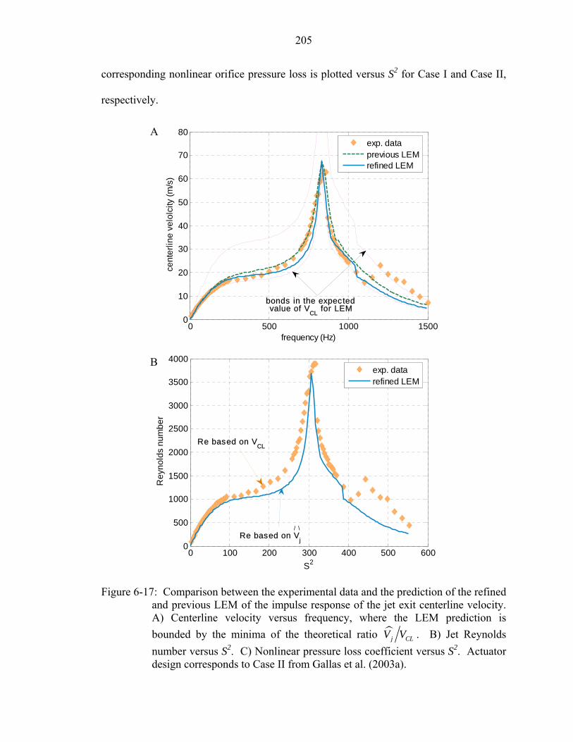
205

corresponding nonlinear orifice pressure loss is plotted versus S2 for Case I and Case II,

respectively.

0 500 1000 15000

10

20

30

40

50

60

70

80

frequency (Hz)

cent

erlin

e ve

lolc

ity (m

/s)

exp. dataprevious LEMrefined LEM

bonds in the expectedvalue of V

CL for LEM

0 100 200 300 400 500 6000

500

1000

1500

2000

2500

3000

3500

4000

S2

Rey

nold

s nu

mbe

r


Re based on VCL

Re based on Vj

/ \

Figure 6-17: Comparison between the experimental data and the prediction of the refined and previous LEM of the impulse response of the jet exit centerline velocity. A) Centerline velocity versus frequency, where the LEM prediction is bounded by the minima of the theoretical ratio j CLV V . B) Jet Reynolds number versus S2. C) Nonlinear pressure loss coefficient versus S2. Actuator design corresponds to Case II from Gallas et al. (2003a).

A

B

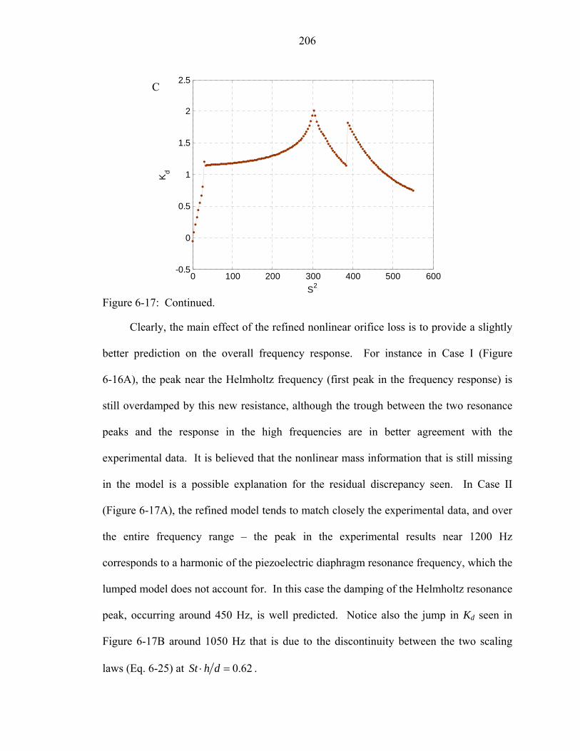
206

0 100 200 300 400 500 600-0.5

0

0.5

1

1.5

2

2.5

S2

Kd


Clearly, the main effect of the refined nonlinear orifice loss is to provide a slightly

better prediction on the overall frequency response. For instance in Case I (Figure

6-16A), the peak near the Helmholtz frequency (first peak in the frequency response) is

still overdamped by this new resistance, although the trough between the two resonance

peaks and the response in the high frequencies are in better agreement with the

experimental data. It is believed that the nonlinear mass information that is still missing

in the model is a possible explanation for the residual discrepancy seen. In Case II

(Figure 6-17A), the refined model tends to match closely the experimental data, and over

the entire frequency range – the peak in the experimental results near 1200 Hz

corresponds to a harmonic of the piezoelectric diaphragm resonance frequency, which the

lumped model does not account for. In this case the damping of the Helmholtz resonance

peak, occurring around 450 Hz, is well predicted. Notice also the jump in Kd seen in

Figure 6-17B around 1050 Hz that is due to the discontinuity between the two scaling

laws (Eq. 6-25) at 0.62St h d⋅ = .

C

207

However, this refined lumped element model fails in predicting some ZNMF

actuator configurations, as shown in Figure 6-18. Although the uncertainty in the

centerline velocity may explain some of the discrepancy, there are yet some deficiencies

in the current lumped model. Some possible explanations would be first on the lack in

the nonlinear mass that is non negligible for low St h d⋅ , which corresponds to the

frequencies above 300 Hz in Figure 6-18B. Similarly, it was shown that, in the time-

domain, the nonlinear term includes the generation of 3ω terms given a forcing at ω.

While this is true in a time-domain, it may not be exactly similar in the frequency domain

method employed above. The amplitude does match for the frequency domain, but the

phase information is incorrect, which affects the impedance prediction via Eq. 6-33. This

is further investigated next.

Figure 6-18: Comparison between the experimental data and the prediction of the refined

and previous LEM of the impulse response of the jet exit centerline velocity. A) Centerline velocity, where the refined LEM prediction is bounded by the minima of the theoretical ratio j CLV V . B) Nonlinear pressure loss coefficient Kd. Actuator design is from Gallas (2002) and is similar to Cases 41 to 50 (h/d = 0.35).

0 500 1000 15000

0.5

1

1.5

2

2.5

frequency(Hz)

B A

Centerline velocity (m/s) Kd

0 500 1000 15000

5

10

15

20

25

30

35

frequency (Hz)

exp dataprevious LEMrefined LEM

bounds in the expectedvalue of VCL for LEM

208

The above analysis is performed on the frequency response of the actuator output.

However, as outlined in Chapter 2, the LEM technique can be easily implemented in the

time domain to then provide the time signals of the jet exit volume flow rate at a single

frequency of operation. Subsequently it can be easily compared with some of the

experimental test cases listed in Table 2-3.

The equation of motion in the time domain of an isolated ZNMF actuator has been

previously derived in Chapter 2 in Eq. 2-29 that is reproduced here for convenience

( )00.5 1 sind d

aO j j j aOlin j jn aC aC n

K SM y y y R y y W tS C C S

ρ ω+ + + = . (6-34)

In the previous lumped model Kd was set to unity, so the second term in the LHS of Eq.

6-34 is a constant. However, Kd is now a function of either St h d⋅ or ( ) Reh d via Eq.

6-25, so that the equation of motion should be rearranged accordingly.

Then, the nonlinear ODE (Eq. 6-34) that describes the motion of the fluid particle

at the orifice is numerically integrated using a 4th order Runge-Kutta algorithm with zero

initial conditions for the particle displacement and velocity, as outlined in Chapter 2, until

a steady state is reached. The results of the jet volume velocity at the orifice exit are

compared with two experimental test cases, namely Case 29 and Case 41, which are

shown in Figure 6-19A and Figure 6-19B, respectively. Again, note that zero phase

corresponds to the onset of the expulsion stroke. While the magnitude of the jet volume

flow rate is clearly well predicted by the refined model, especially for Case 41 (Figure

6-19B), the distortion seen in Case 29 (Figure 6-19A) is not captured by the low-order

model that remains nearly sinusoidal. The distortions in the signal are presumably due to

the phase distortions that are not completely accounted for in this refined model. Note

209

that at this particular frequency the frequency domain method described above gives a

similar value for the jet volume flow rate amplitude.

0 45 90 135 180 225 270 315 360-4

-3

-2

-1

0

1

2

3

4

5x 10

-5

phase (degree)


0 45 90 135 180 225 270 315 360-2.5

-2

-1.5

-1

-0.5

0

0.5

1

1.5

2

2.5x 10

-6

phase (degree) Figure 6-19: Comparison between the refined LEM prediction and experimental data of

the time signals of the jet volume flow rate. A) Case 29: S = 34, Re = 1131, St = 1.1, h/d = 0.95. B) Case 41: S = 12, Re = 40.6, St = 3.49, h/d = 0.35.

In conclusion, a refined lumped element model as been presented to predict the

response of an isolated ZNMF actuator. The model builds on a control volume analysis

A Je

t vol

ume

flow

rate

(m3 /s

) Je

t vol

ume

flow

rate

(m3 /s

)

B

210

of the unsteady orifice flow to yield an expression of the dimensionless pressure drop

across the orifice as a function of the Reynolds number Re, Strouhal number St and

orifice aspect ratio h/d. The model was validated via numerical simulations, and then a

scaling law of the orifice pressure loss was developed based on experimental data. Next,

the refined pressure loss coefficient was implemented into the existing low-dimensional

lumped element model that predicts the actuator output. The new model was then

compared with some experimental test cases in both the frequency and time domain.

This refined model is able to reasonably predict the magnitude of the jet velocity. Notice

however that this model can be applicable to any type of ZNMF devices, meaning the

driver and cavity of the actuator are well modeled, the only refinement made being for

the orifice flow. And as seen in Chapter 4, it exhibits a rich and complex dynamics

behavior that the refined model developed above is in essence able to capture, while still

lacking in the details. Clearly, the reduced-order model as presented in this chapter will

greatly beneficiate from a larger available high quality database, both numerically and

experimentally.

211

CHAPTER 7

ZERO-NET MASS FLUX ACTUATOR INTERACTING WITH AN EXTERNAL BOUNDARY LAYER

This chapter is dedicated to the interaction of a ZNMF actuator with an external

boundary layer, in particular with a laminar, flat-plate, zero pressure gradient (ZPG)

boundary layer. First, a qualitative discussion is provided concerning grazing flow

interaction effects. This discussion is based on the numerical simulations performed by

Rampuggoon (2001) for the case of a ZNMF device interacting with a Blasius laminar

boundary layer and also on studies of other applications such as acoustic liners. Next, the

nondimensional analysis performed in Chapter 2 for the case of an actuator issuing into

ambient air is extended to include the grazing flow interaction effects. Based on these

results, two approaches to develop reduced-order models are proposed and discussed.

One model builds on the lumped element modeling technique that was previously applied

to an isolated device and leverages the semi-empirical models developed in the acoustic

liner community for grazing flow past Helmholtz resonators. Next, two scaling laws for

the exit velocity profile behavior are developed that are based on available computational

data. Each model is developed and discussed, and the effects of several key parameters

are investigated.

On the Influence of Grazing Flow

As mentioned in Chapter 1, most applications of ZNMF devices involve an external

boundary layer. Intuitively, the performance of a ZNMF actuator will be strongly

affected by some key grazing flow parameters that need to be identified. Rampuggoon

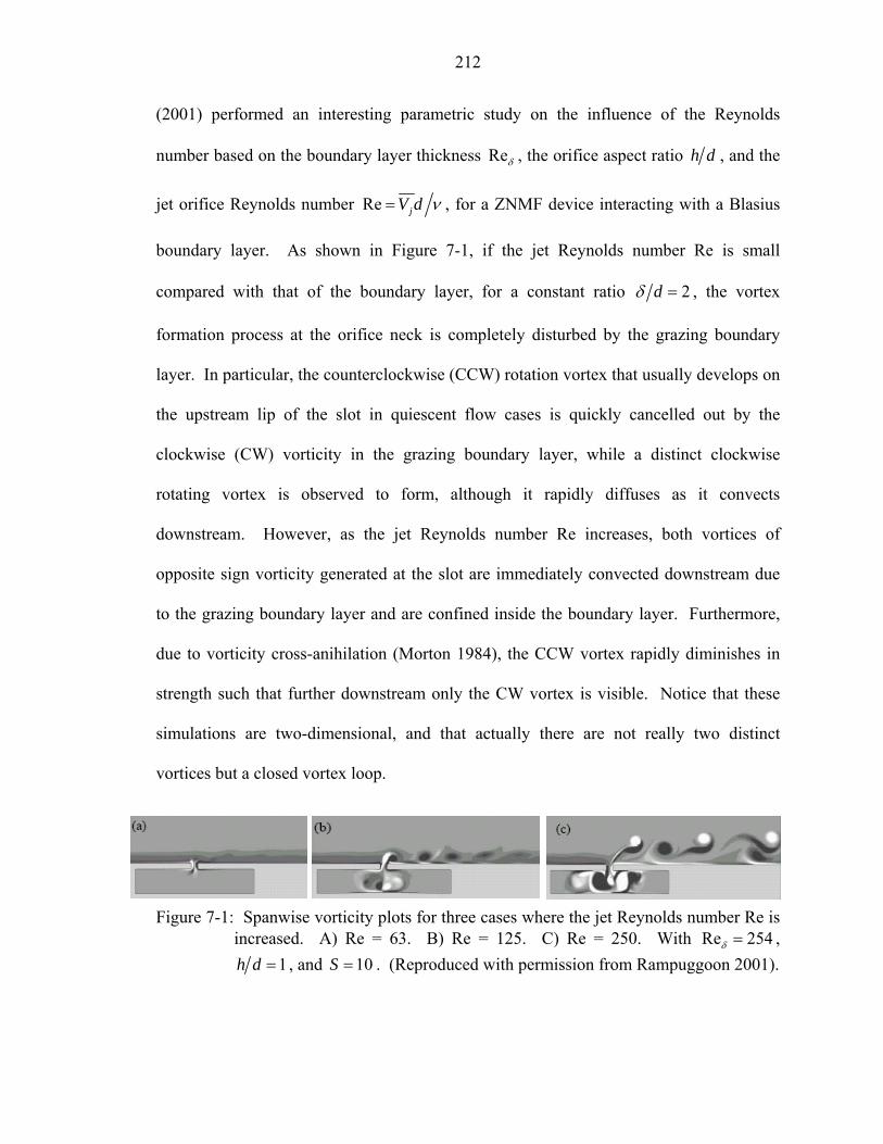
212

(2001) performed an interesting parametric study on the influence of the Reynolds

number based on the boundary layer thickness Reδ , the orifice aspect ratio h d , and the

jet orifice Reynolds number Re jV d ν= , for a ZNMF device interacting with a Blasius

boundary layer. As shown in Figure 7-1, if the jet Reynolds number Re is small

compared with that of the boundary layer, for a constant ratio 2dδ = , the vortex

formation process at the orifice neck is completely disturbed by the grazing boundary

layer. In particular, the counterclockwise (CCW) rotation vortex that usually develops on

the upstream lip of the slot in quiescent flow cases is quickly cancelled out by the

clockwise (CW) vorticity in the grazing boundary layer, while a distinct clockwise

rotating vortex is observed to form, although it rapidly diffuses as it convects

downstream. However, as the jet Reynolds number Re increases, both vortices of

opposite sign vorticity generated at the slot are immediately convected downstream due

to the grazing boundary layer and are confined inside the boundary layer. Furthermore,

due to vorticity cross-anihilation (Morton 1984), the CCW vortex rapidly diminishes in

strength such that further downstream only the CW vortex is visible. Notice that these

simulations are two-dimensional, and that actually there are not really two distinct

vortices but a closed vortex loop.

Figure 7-1: Spanwise vorticity plots for three cases where the jet Reynolds number Re is

increased. A) Re = 63. B) Re = 125. C) Re = 250. With Re 254δ = , 1h d = , and 10S = . (Reproduced with permission from Rampuggoon 2001).

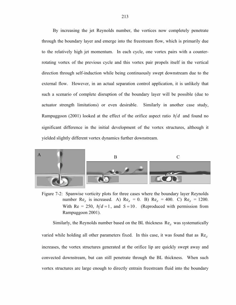
213

By increasing the jet Reynolds number, the vortices now completely penetrate

through the boundary layer and emerge into the freestream flow, which is primarily due

to the relatively high jet momentum. In each cycle, one vortex pairs with a counter-

rotating vortex of the previous cycle and this vortex pair propels itself in the vertical

direction through self-induction while being continuously swept downstream due to the

external flow. However, in an actual separation control application, it is unlikely that

such a scenario of complete disruption of the boundary layer will be possible (due to

actuator strength limitations) or even desirable. Similarly in another case study,

Rampuggoon (2001) looked at the effect of the orifice aspect ratio h d and found no

significant difference in the initial development of the vortex structures, although it

yielded slightly different vortex dynamics further downstream.

Figure 7-2: Spanwise vorticity plots for three cases where the boundary layer Reynolds

number Reδ is increased. A) Reδ = 0. B) Reδ = 400. C) Reδ = 1200. With Re = 250, 1h d = , and 10S = . (Reproduced with permission from Rampuggoon 2001).

Similarly, the Reynolds number based on the BL thickness Reδ was systematically

varied while holding all other parameters fixed. In this case, it was found that as Reδ

increases, the vortex structures generated at the orifice lip are quickly swept away and

convected downstream, but can still penetrate through the BL thickness. When such

vortex structures are large enough to directly entrain freestream fluid into the boundary

A B C

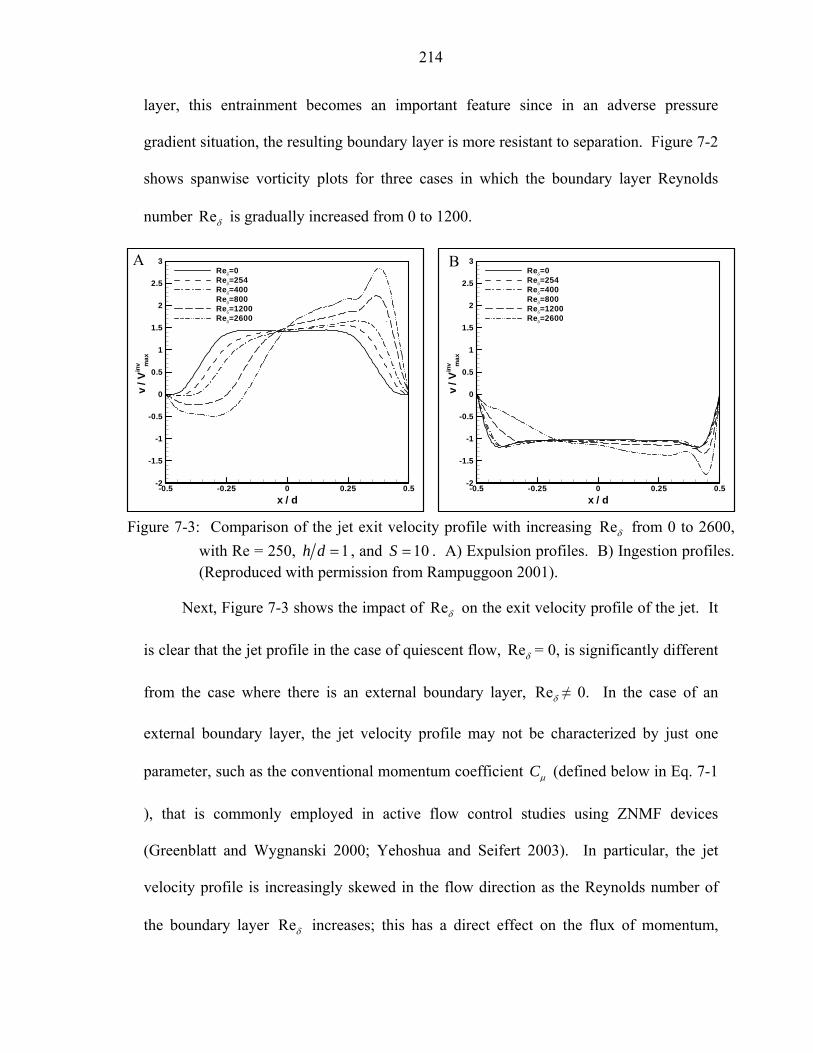
214

layer, this entrainment becomes an important feature since in an adverse pressure

gradient situation, the resulting boundary layer is more resistant to separation. Figure 7-2

shows spanwise vorticity plots for three cases in which the boundary layer Reynolds

number Reδ is gradually increased from 0 to 1200.

x / d

v/V

inv m

ax

-0.5 -0.25 0 0.25 0.5-2

-1.5

-1

-0.5

0

0.5

1

1.5

2

2.5

3Reδ=0Reδ=254Reδ=400Reδ=800Reδ=1200Reδ=2600

x / d

v/V

inv m

ax

-0.5 -0.25 0 0.25 0.5-2

-1.5

-1

-0.5

0

0.5

1

1.5

2

2.5

3Reδ=0Reδ=254Reδ=400Reδ=800Reδ=1200Reδ=2600

Figure 7-3: Comparison of the jet exit velocity profile with increasing Reδ from 0 to 2600, with Re = 250, 1h d = , and 10S = . A) Expulsion profiles. B) Ingestion profiles. (Reproduced with permission from Rampuggoon 2001).

Next, Figure 7-3 shows the impact of Reδ on the exit velocity profile of the jet. It

is clear that the jet profile in the case of quiescent flow, Reδ = 0, is significantly different

from the case where there is an external boundary layer, Reδ ≠ 0. In the case of an

external boundary layer, the jet velocity profile may not be characterized by just one

parameter, such as the conventional momentum coefficient Cµ (defined below in Eq. 7-1

), that is commonly employed in active flow control studies using ZNMF devices

(Greenblatt and Wygnanski 2000; Yehoshua and Seifert 2003). In particular, the jet

velocity profile is increasingly skewed in the flow direction as the Reynolds number of

the boundary layer Reδ increases; this has a direct effect on the flux of momentum,

B A

215

vorticity, and energy from the slot. Therefore, from the point of view of parameterization

of the jet velocity profile, the skewness appears to be an important parameter that should

be considered, and is introduced in the next section. Similarly, it was shown (Utturkar et

al. 2002) that the momentum coefficient differs during the ingestion versus the expulsion

portion of the stroke and both are different from the ambient case.

The above discussion permits one to gain significant insight on the influence of

several key dimensionless parameters on the overall behavior of a ZNMF actuator

interacting with an external boundary layer. However, Rampuggoon’s study was limited

to the special case of a Blasius boundary layer, which is an incompressible, laminar, zero

pressure gradient boundary layer over a flat plate. Hence, a further discussion is provided

below based on the work performed on flow past Helmholtz resonators over a wider

range of flow conditions.

As previously discussed in Chapter 1, research involving flow-induced resonators

has been mainly triggered by the desire to suppress oscillations, such as those occurring

for example on automobile sunroofs (Elder 1978; Meissner 1987), or in sound absorbing

devices, such as mufflers (Sullivan 1979) or acoustic liners in engine nacelles (Malmary

et al. 2001). Others have also suggested that an array of Helmholtz resonators driven by

a grazing flow can modify a turbulent boundary layer (Flynn et al. 1990). Even though

these flow-induced resonators are passive, as compared to active ZNMF actuators, their

major findings are of interest and warrant a discussion. It should also be noted that the

key parameter that has been widely used by researchers to quantify the interaction

between the acoustic field and the grazing flow at the orifice exit is the specific acoustic

216

impedance of the treated surface. Conveniently, this is similar to that of our previous

research for isolated ZNMF actuators in using LEM.

Choudhari et al. (1999) performed an interesting study by comparing their

numerical simulation results of flow past a Helmholtz resonator to published

experimental data. Three different configurations for the resonator were studied, as listed

in Table 7-1. The two-dimensional or axisymmetric laminar compressible Navier-Stokes

equations were solved using an-house, node-based finite volume Cartesian grid solver.

When applicable, a turbulent model was used based on the one-equation Spalart-Allmaras

model (Spalart and Allmaras 1992). The reader is referred to their paper for a discussion

of the numerical scheme that was employed. Although not reproduced here, the

numerical simulations compared well, both qualitatively and quantitatively, with the

experimental data from Hersh and Walker (1995) and Melling (1973).

Table 7-1: List of configurations used for impedance tube simulations used in Choudhari et al. (1999).

Reference

Orifice diameter

(or width) ( )d mm

Thickness to

diameter ratio h d

Open area ratio

( )%σ

Acoustic amplitude

( )SPL dB

Cavity height ( )H mm

Freq. ( )f Hz

Hersh & Walker (1995) Single circular orifice

9.52

1.33

3.5

95 126

22.23**

250-600

Melling (1973) Perforate 153 A/00

1.27

0.5

7.5

114 162*

25.4 4λ=

3400

LaRC (1998-1999) Slot Perforate

2.54 2.54

1 2.5

5 5

linear 114 148*

76.2 76.2 4λ=

566 1139

*Free space SPL **Tuned for 500f Hz=

As previously discussed in Chapter 4, although incomplete in terms of essential

dimensionless parameters, two different regimes were identified in terms of the sound

217

pressure level (SPL): one for low-amplitude that is termed “linear” and one for high

acoustic amplitude it is nonlinear. The computation from Choudhari et al. (1999) showed

that in the linear regime, the fully-developed unsteady pipe flow theory applied to

perforates with an ( )1O aspect ratio h d gave reasonable estimates, although the flow

near the orifice edges is dominated by the rapid acceleration around the corners. Also,

they were able to show that the dissipation occurring in the orifice is mainly due to

viscous effects rather than thermal dissipation. In the nonlinear regime, clear distortion

in the probe signals (pressure fluctuation, orifice velocity) are present as already shown in

the first part of Chapter 5 in Figure 5-9. When a laminar boundary layer interacts with

the liner surface, as shown in Figure 7-4, the inflow part of the cycle exhibits a narrower

“vena contracta” than for the outflow phase. This supports the hypethesis reported in

earlier experimental studies (e.g., Budoff and Zorumski 1971) that, in the presence of

grazing flow, the resistance to blowing into the flow is significantly less than the

resistance to suction from the stream. Physically, this is equivalent in comparing the

expulsion phase from a “quiescent medium” inside the resonator to the ingestion phase

that directly interacts with a grazing flow. Such a result is relevant and should be taken

into account when modeling a ZNMF actuator.

Therefore, from the study of previous work performed in aerodynamics as well as

in aeroacoustics, some main features of the interaction of a grazing flow with a

Helmholtz resonator and/or a ZNMF actuator can be extracted that yield more insight

into the flow physics of such complex interaction behavior. In this regard, a

nondimensional analysis is first described below, followed by the development of

physics-based reduced-order models.

218

Figure 7-4: Pressure contours and streamlines for mean A) inflow, and B) outflow through a resonator in the presence of grazing flow (laminar boundary layer at Re 3120δ = , 1dδ ≈ , 0.5h d ≈ , and average inflow/outflow velocity 10%≈ of grazing velocity). (Reproduced with permission from Choudhari et al. 1999)

Dimensional Analysis

In Chapter 2, the actuator output parameters of interest were identified and defined

from the time- and spatial-averaged jet velocity jV during the expulsion portion of a

cycle defined in Eq. 2-4. Examples of such quantities are the jet Reynolds number Re, or

amplitude of the jet output volume flow rate jQ . Another quantity of interest in the case

of a grazing boundary layer is the oscillatory momentum coefficient. In the presence of a

grazing boundary layer, to quantify the addition of momentum by the actuator and

following the definition suggested by Greenblatt and Wygnanski (2000), the total (mean

plus oscillatory) momentum coefficient of the periodic excitation is defined as the ratio of

the momentum flux of the jet to the freestream dynamic pressure times a reference area.

For a 2-D slot,

2rms

21 2j n

ref

u SC

U Sµ

ρρ∞ ∞

= , (7-1)

219

where the subscript j refers to the jet, nS d w= × is the slot area, refS L w= × is a

reference area with L being any relevant length scale of either the airfoil model or the

grazing BL (chord length c, boundary layer momentum thickness θ , displacement

thickness δ ∗ , etc.). Notice that since no net mass is injected from the jet to the exterior

medium (indeed, the jet is “synthesized” from the working ambient fluid), and if the

turbulent boundary layer is assumed incompressible along with the flow through the

orifice, then no significant density variations are expected, neither in the incoming

boundary layer nor in the jet orifice. Therefore the fluid density of the jet can be

considered as the same as the ambient fluid, i.e. jρ ρ∞≅ . Similarly, even though the jet

velocity contains both mean and oscillatory components, here only the oscillatory part of

Cµ is retained since the mean component is identically zero for a zero-net mass flux

device. Thus, for incompressible flow and after time-averaging, the momentum

coefficient is defined as

2rms2

2u dCUµ θ∞

= , (7-2)

where 2rmsu is the mean square value of the oscillatory jet velocity normal component, and

the boundary layer momentum thickness θ is chosen as the relevant local boundary layer

length scale. Based on the experimental results on the orifice flow described in Chapter

4, a clear distinction between the ejection and the ingestion part of the cycle exists. Thus,

the momentum coefficient defined in Eq. 7-2 can be rewritten such as

, ,ex inC C Cµ µ µ= + , (7-3)

220

where the subscripts “ex” and “in” refer to, respectively, the expulsion and ingestion

portions of the cycle.

Yet other parameters, such as energy or vorticity flux, etc. might also play an

important role in determining the effect of the jet on the boundary layer, not limiting

ourselves to the momentum coefficient as in previous studies (Amitay et al. 1999; Seifert

and Pack 1999; Yehoshua and Seifert 2003). In this current work, a more general

approach to characterizing the jet behavior via successive moments of the jet velocity

profile is thus advocated, following Rampuggoon (2001). The nth moment of the jet is

defined as 12 12

n njCφ φ

= V , where jV is the jet velocity normalized by a suitable velocity

scale (e.g., freestream velocity) and 12φ

⋅ represents an integral over the jet exit plane and

a phase average of njV over a phase interval from 1φ to 2φ . This leads to the following

expression

( )2

1212 1

1 1 ,n

nnj nS

n

C t x d dSS

φ

φ φφ

φ φ⎡ ⎤= ⎣ ⎦− ∫ ∫ V . (7-4)

Note the similarity with the definition of the jet velocity jV given by Eq. 2-4

previously defined, where one period of the cycle and the phase interval are related by

2 1T φ φ= − , and the normalized jet velocity is related by

( ) ( ),, j

j

v t xt x

U∞

=V , (7-5)

if one takes, for instance, the freestream velocity U∞ as a suitable velocity scale.

As observed from the discussion above, preliminary simulations (Rampunggoon

2001; Mittal et al. 2001) indicate that the jet velocity profile is significantly different

221

during the ingestion and expulsion phases in the presence of an external boundary layer.

Defining the moments separately for the ingestion and expulsion phases, they are denoted

by ninC and n

exC , respectively. Furthermore, it should be noted that this type of

characterization is not simply for mathematical convenience, since these moments have

direct physical significance. For example, 1 1in exC C+ corresponds to the jet mass flux

(which is identically equal to zero for a ZNMF device). The mean normalized jet

velocity during the expulsion phase is 1exC . Furthermore, 2 2

in exC C+ corresponds to the

normalized momentum flux of the jet, while 3 3in exC C+ represents the jet kinetic energy

flux. Finally, for n →∞ , ( )1/ nnexC corresponds to the normalized maximum jet exit

velocity.

In addition to the moments, the skewness or asymmetry of the velocity profile

about the center of the orifice is found to be useful (see Rampuggoon 2001) and can be

estimated as

( ) ( )2

121

2

02 1

1 1 , ,2

d

j jX x x d dxd

φ

φ φφ φ φ

φ φ⎡ ⎤= − −⎣ ⎦− ∫ ∫ V V . (7-6)

Assuming the external boundary layer to be flowing in the positive x direction, if

120Xφ > the jet velocity profile is skewed towards the positive x, i.e. the jet has higher

velocity in the downstream portion of the orifice than in its upstream part, while for

120Xφ < the trend is inversed. If

120Xφ = , the jet velocity profile is symmetric about the

orifice center in an average sense, which would, for example, correspond to the no-

grazing flow or ambient case. Similarly, the flux of vorticity can be defined as (Didden

1979),

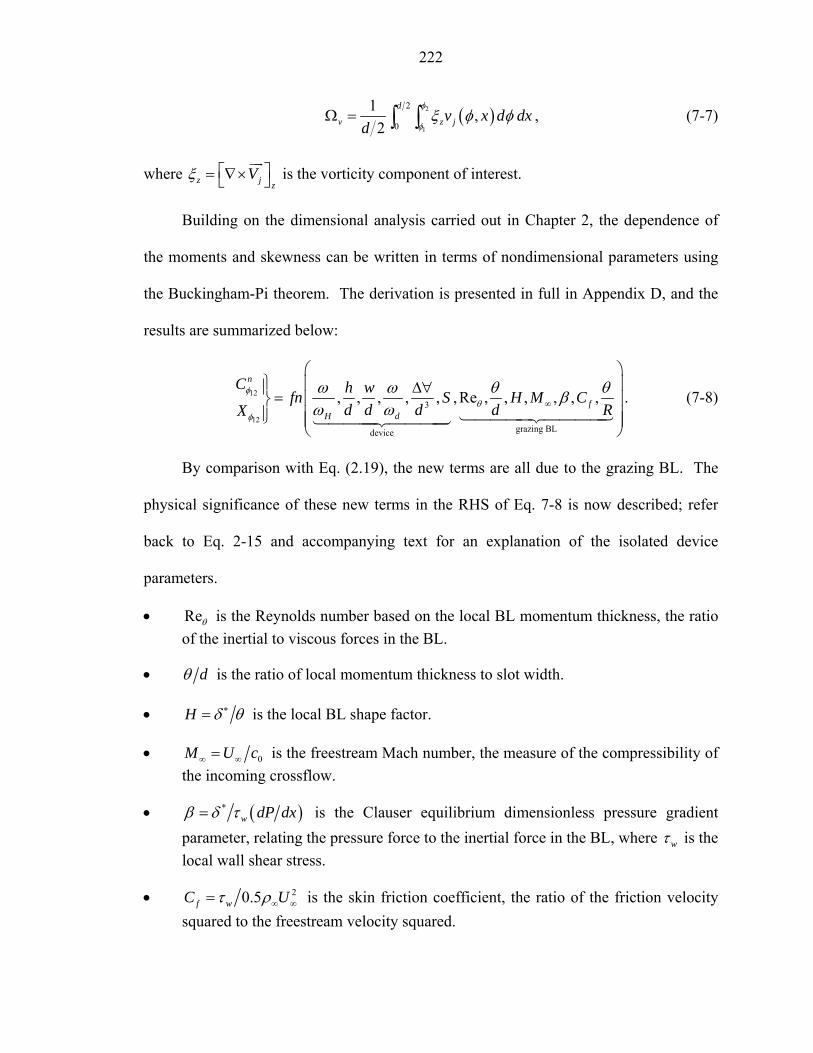
222

( )2

1

2

0

1 ,2

d

v z jv x d dxd

φ

φξ φ φΩ = ∫ ∫ , (7-7)

where z j zVξ ⎡ ⎤= ∇×⎣ ⎦ is the vorticity component of interest.

Building on the dimensional analysis carried out in Chapter 2, the dependence of

the moments and skewness can be written in terms of nondimensional parameters using

the Buckingham-Pi theorem. The derivation is presented in full in Appendix D, and the

results are summarized below:

12

12

3

grazing BLdevice

, , , , , , Re , , , , , ,n

fH d

C h wfn S H M Cd d d d RX

φθ

φ

ω ω θ θβω ω ∞

⎛ ⎞⎫ ⎜ ⎟∆∀⎪ = ⎜ ⎟⎬⎪ ⎜ ⎟⎭ ⎜ ⎟

⎝ ⎠

. (7-8)

By comparison with Eq. (2.19), the new terms are all due to the grazing BL. The

physical significance of these new terms in the RHS of Eq. 7-8 is now described; refer

back to Eq. 2-15 and accompanying text for an explanation of the isolated device

parameters.

• Reθ is the Reynolds number based on the local BL momentum thickness, the ratio of the inertial to viscous forces in the BL.

• dθ is the ratio of local momentum thickness to slot width.

• H δ θ∗= is the local BL shape factor.

• 0M U c∞ ∞= is the freestream Mach number, the measure of the compressibility of the incoming crossflow.

• ( )*w dP dx=β δ τ is the Clauser equilibrium dimensionless pressure gradient

parameter, relating the pressure force to the inertial force in the BL, where wτ is the local wall shear stress.

• 20.5f wC Uτ ρ∞ ∞= is the skin friction coefficient, the ratio of the friction velocity squared to the freestream velocity squared.

223

• Rθ is the ratio of the local momentum thickness to the surface of curvature.

Notice that the parameters based on the BL momentum thickness have been

selected versus the BL thickness or displacement thickness, by analogy with the LEM-

based low dimensional models developed in this dissertation. Also, it is fairly obvious

that the parameter space for this configuration is extremely large and some judicious

choices have to be made to simplify the parametric space. For instance, in the case of a

ZNMF actuator interacting with an incompressible, zero pressure gradient laminar

boundary layer (i.e., a Blasius boundary layer), the functional form of Eq. 7-8 takes the

form

12

12

3

Blasius

, , , , , , Re ,n

H d

C h wfn Sd d d dX

φθ

φ

ω ω θω ω

⎫ ⎛ ⎞∆∀⎪ =⎬ ⎜ ⎟⎝ ⎠⎪⎭

, (7-9)

which is the situation for which the low-order models described next are restricted to.

Reduced-Order Models

From the discussion provided in the previous sections, two approaches can be

sought to characterize the interaction of a ZNMF actuator with an external boundary

layer. One approach is an extension of the lumped element model to account for the

grazing flow on the orifice impedance. However, this method does not provide any

details regarding the velocity profile. A second approach is thus to develop a scaling law

of the velocity profile at the orifice exit and its integral parameters that will represent the

local interaction of the ZNMF actuator with the incoming grazing boundary layer. Both

of these are discussed below.

224

Lumped Element Modeling-Based Semi-Empirical Model of the External Boundary Layer

Definition

As a first model, the LEM technique previously introduced, described, and

validated for a ZNMF actuator exhausting into still air is extended to include the effect of

a grazing boundary layer. Figure 7-5 shows a typical LEM equivalent circuit

representation of a generic ZNMF device interacting with a grazing boundary layer,

where the parameters are specified in the acoustic domain (as denoted by the first letter a

in the subscript). The boundary layer impedance is introduced in series with the orifice

impedance, since they share the same volume flow rate jQ , the ZNMF actuator

exhausting into the grazing boundary layer.

ZaD

Z aC

Qd-Qj

Qd Qj

existing modelcrossflowaddition

∆Pc

ZaOZ aB

L

Figure 7-5: LEM equivalent circuit representation of a generic ZNMF device interacting with a grazing boundary layer.

For clarification, each component of the equivalent circuit shown in Figure 7-5 is

briefly summarized below. First, the acoustic driver impedance aDZ is inherently

dependant on the dynamics of the utilized driver, although the volumetric flow rate dQ

that it generates can be generalized to be equal to

( )0 sind dQ j j S W t= ∆∀=ω ω ω . (7-10)

225

The acoustic impedance of the cavity is modeled as an acoustic compliance

1caC

d j aC

PZQ Q j Cω∆

= =−

, (7-11)

where the cavity acoustic compliance is given by

20

aCCcρ∀

= . (7-12)

Then, the acoustic impedance of the orifice is defined by (see previous Chapter for

details)

, ,aO aO lin aO nl aOZ R R j Mω= + + , (7-13)

where the linear acoustic resistance ,aO linR corresponds to the viscous losses in the orifice

and is set to be

aOlin aNR R= , (7-14)

which takes a different functional form depending on the orifice geometry as described in

Chapter 2 and Appendix E. As discussed in Chapter 2 and in great detail in Chapter 6,

the nonlinear acoustic resistance ,aO nlR represents the nonlinear losses due to the

momentum integral and is given by

, 2

0.5 d jaO nl

n

K QR

Sρ

= , (7-15)

where dK is the nonlinear pressure drop coefficient that is a function of the orifice shape,

Stokes number and jet Reynolds number (see Chapter 6 for details). Finally, the acoustic

orifice mass aOM groups the effect of the mass loading (or inertia effect) aNM and that of

the acoustic radiation mass aRadM , such that

aO aN aRadM M M= + , (7-16)

226

where again each quantity is a function of the orifice geometry (see Appendix E).

The new term is the acoustic boundary layer impedance, which takes the form

aBL aBL aBLZ R jX= + , (7-17)

where the acoustic resistance aBLR and reactance aBLX will be defined further below.

The total acoustic impedance of the orifice, including the grazing boundary layer effect is

then defined by

,c

aO t aO aBLj

PZ Z ZQ∆

= + = . (7-18)

where the boundary layer impedance is in series with the isolated orifice impedance since

they share a common flow. Note that in the ZNMF actuator lumped element model, the

pressure inside the cavity cP∆ is equal to the pressure drop across the orifice (see

discussion on the pressure field in Chapter 5). Also, the radiation impedance of the

orifice is modeled as a circular (rectangular) piston in an infinite baffle for an

axisymmetric (rectangular) orifice, and only the mass contribution is taken into account,

since at low wavenumbers, kd , the radiation resistance term is almost negligible

(Blackstock 2000, p. 459).

The goal here is to find an analytical expression for the acoustic grazing boundary

layer impedance aBLZ that will capture the main contributions of the grazing boundary

layer, i.e. increase the resistance of the orifice and reduce the effective mass oscillating in

the orifice. From the dimensionless analysis carried out in Chapter 2 and in the previous

section, a large parameter space has been revealed that should be sampled.

Based on the acoustic liner literature reviewed in Chapter 1 and Appendix A, the

so-called NASA Langley ZKTL (Betts 2000) is first implemented in the application of a

227

ZNMF device to extract a simple analytical expression. Specifically, the impedance

model is derived from the boundary conditions used in the ZKTL impedance model (see

Eqs. A-12 and A-13), which finds its origins in the work done by Hersh and Walker

(1979), Heidelberg et al. (1980) for the resistance part, and by Rice (1971) and Motsinger

and Kraft (1991) for the reactance part of the impedance. With slight modifications and

rearrangements discussed below, the model is extended to the present problem to yield

the following impedance model in the acoustic domain

( )

0

2 1.256aBL

n

c MRS

d

ρδ

∞=+

, (7-19)

for the acoustic resistance part and

03

1 0.851 305aBL

n D

c kdXS C Mρ

∞

=+

, (7-20)

to characterize the acoustic reactance of the grazing impedance. The quantity 0 nc Sρ

corresponds to the characteristic acoustic impedance of the medium and is used for

normalization to express the results in the acoustic domain, DC is the orifice discharge

coefficient that has been previously introduced, and 0 0.96 nh S= is an orifice end

correction (see Appendix B for details). Notice that the original expressions, Eqs. A-12

and A-13, are functions of the porosity factor. However, the resistance part was

originally derived from first principles for a single orifice (Hersh and Walker 1979) and

then extended to an array of independent orifices (hence perforated plate) via the simple

relation

0, single orifice0, perforate

ZZ

σ= , (7-21)

where the porosity is defined by

228

( )holes hole areatotal area

Nσ

×= , (7-22)

and holesN is the number of holes in the perforate. Eq. 7-21 is applicable when assuming

that the orifices are not too close to each other in order to alleviate any interactions

between them. Ingard (1953) states that the resonators can be treated independently of

each other if the distance between the orifices is greater than half of the acoustic

wavelength. This statement can be related to the discussion in Chapter 4 on the influence

of the dimensionless stroke length. The porosity factor in the resistance expression of Eq.

A-12 can then be disregarded to yield Eq. 7-19. Similarly, the end correction

0.85 1 0.7 dσ⎡ ⎤−⎣ ⎦ in the reactance expression from Eq. A-13 is found from Ingard

(1953) when perforate plates are used and should be compared with the single orifice end

correction 0.85d for a circular orifice (see Appendices A and B). Thus, the acoustic

reactance due to the grazing flow effect takes the form of Eq. 7-20.

It is worthwhile to note that the boundary layer model in its present form is

primarily a function of the grazing flow Mach number M∞ , the ratio between the orifice

diameter and the acoustic wavelength 2kd dπ λ= , and the ratio of the boundary layer

thickness to the orifice diameter dδ , the latter mainly limiting the resistance

contribution. Also, the orifice effect is represented by the discharge coefficient DC in the

reactance expression. Furthermore, it is sometimes useful to denote the specific

reactance in terms of the effective length 0h , such that

0 0X hρω= . (7-23)

229

From Eq. 7-20 and Eq. 7-23, it can be seen that when the specific reactance is

normalized by the orifice area, it yields the reactance expression in the acoustic domain.

The effect of the grazing boundary layer tends to decrease the “no crossflow” orifice

effective length 0 0.96 nh S (see Appendix B for a complete definition of 0h ) by the

quantity ( )31 305DC M∞+ , which is a function of the orifice shape, flow parameters, and

freestream Mach number.

Before directly implementing this grazing boundary layer impedance into the full

lumped element model of a ZNMF actuator and observing its effect on the device

behavior, the model is compared to previous data for flow past Helmholtz resonators in

order to validate it.

Boundary layer impedance implementation in Helmholtz resonators

In Appendix A, five different models of grazing flow past Helmholtz resonators are

presented in detail, and Table A-1 summarizes the operating conditions. A large

variation in operating conditions for a range of applications is considered. However, in

the process of gathering suitable data to compare the impedance model presented above,

two main difficulties appeared:

• First, proper documentation of the experimental setup and operating conditions (especially the grazing BL) is often deficient. Therefore, some available experimental databases were not used because one or more variable definitions were lacking.

• Second, since practical applications of acoustic liners often deal with a thin face sheet perforate, the orifice ratio h d is usually much less than unity. As seen from the results of modeling of a ZNMF actuator in a quiescent medium, this can yield complex orifice flow patterns and thus represents a limiting case of 0h d → in the impedance model.

230

Nonetheless, two datasets from two different publications were found to suit our

purpose. The first database comes from the extensive experimental study performed by

Hersh and Walker (1979). Only the thick orifice investigation is used here in order to

fulfill the model assumption of 1h d ≥ . The two-microphone impedance test data is

summarized herein for the five orifice resonator configurations described in Table 7-2.

The complete dataset can be found in Hersh and Walker (1979), and Figure A-2 in

Appendix A gives the schematic of the test apparatus that was used. It is basically an

effort divider, as shown in Figure 7-6.

Table 7-2: Experimental operating conditions from Hersh and Walker (1979). Resonator

model ( )cD mm ( )H mm ( )d mm ( )h mm h d

1 31.75 12.7 1.78 0.51 0.28 2 “ “ “ 1.01 0.57 3 “ “ “ 1.03 1.14 4 “ “ “ 4.06 2.28 5 “ “ “ 8.13 4.56

2 2cd Dσ = ( )f Hz ( )T K∞ ( )P kPa∞ dδ

1 0.003 552 292.04 101.93 4.8 2 “ 530 295.93 101.83 “ 3 “ 414 292.04 100.07 “ 4 “ 333 297.04 101.93 “ 5 “ 255 296.48 101.93 “

ZaO

Pi

Qj

Z aC

ZaBL

Pc

effort divider

Figure 7-6: Schematic of an effort divider diagram for a Helmholtz resonator.

231

The data is presented for different values of incident pressure iP and grazing flow

velocity U∞ in terms of the total resonator area-averaged specific resistance and

reactance normalized by the specific medium impedance, respectively 0 0R cρ and

0 0X cρ . The resistance and reactance were computed by measuring the amplitude of

the incident iP and cavity cP sound waves, and also by measuring the phase difference

between the incident sound field and the cavity sound field icφ . These values are

substituted into Eqs. 7-24 and 7-26 given below, respectively, for the resistance and

reactance

( ) ( )

( )

SPL SPL0 20

0 0

sin10sin

i cicR

c H cφσ

ρ ω

−⎡ ⎤= ⎢ ⎥

⎢ ⎥⎣ ⎦, (7-24)

following the effort divider depicted in Figure 7-6,

1 1

0

0

Re Rec aCnC nC

i aO aBL aC

R P ZZ Zc P Z Z Zρ

− −⎧ ⎫ ⎧ ⎫⎛ ⎞ ⎛ ⎞⎪ ⎪ ⎪ ⎪= =⎨ ⎬ ⎨ ⎬⎜ ⎟ ⎜ ⎟+ +⎝ ⎠ ⎝ ⎠⎪ ⎪ ⎪ ⎪⎩ ⎭ ⎩ ⎭, (7-25)

and

( ) ( )

( )

SPL SPL0 20

0 0

cos10sin

i cicX

c H cφσ

ρ ω

−⎡ ⎤= ⎢ ⎥

⎢ ⎥⎣ ⎦, (7-26)

where ( ) ( )SPL SPLi c− represents the sound pressure level difference (in dB ) between

the incident sound field and the cavity sound field, H is the cavity depth of the resonator,

n cS Sσ = is an averaged area (ratio of the orifice-to-cavity cross sectional area), and

nCZ is the area-averaged normalized acoustic cavity impedance such that

0

nnC aC

SZ Zc

σρ

⎛ ⎞= ⎜ ⎟

⎝ ⎠, (7-27)

232

0nS cρ being the characteristic impedance of the medium in the acoustic domain.

For each resonator tested, the frequency was adjusted to achieve resonance at

70iP dB= and 0U∞ = , by seeking the frequency for which the phase difference between

the incident and cavity sound pressure fields were 90o. The results presented hereafter

are from the five orifice models as listed in Table 7-2. The normalized area-averaged

impedance, defined by jζ θ χ= + for a single orifice, as a function of the grazing flow

Mach number are plotted in Figure 7-7A to Figure 7-7E. Specifically, the total specific

resistance 0R of the resonator is normalized by the characteristic impedance of the

medium 0cρ , and the cavity reactance is subtracted from the total resonator reactance

such that

0 , 0 ,0 0

0 0 0 0 0

cotO t O tCX XX X Hc c c c c

ωσρ ρ ρ ρ

⎛ ⎞= + = − ⎜ ⎟

⎝ ⎠, (7-28)

where 0OX is the specific orifice reactance that includes the inertia effect and the BL

contribution,

( )0

0

cotCX kHc

σρ

= − (7-29)

is the normalized specific reactance of the cavity, and 0k cω= is the wavenumber.

Notice that Eq. 7-29 is similar to the definition of the acoustic cavity impedance aCZ

given by Eqs. 7-11 and 7-12, since for 1kH the Maclaurin series expansion of the

cotangent function can be truncated to its first term, such that

( )13 3

0 0

0

cot ...3

CX ck HkH kHc H

σ σ σρ ω

−⎛ ⎞

= − = − + − −⎜ ⎟⎝ ⎠

, (7-30)

and the normalized acoustic cavity impedance is given by

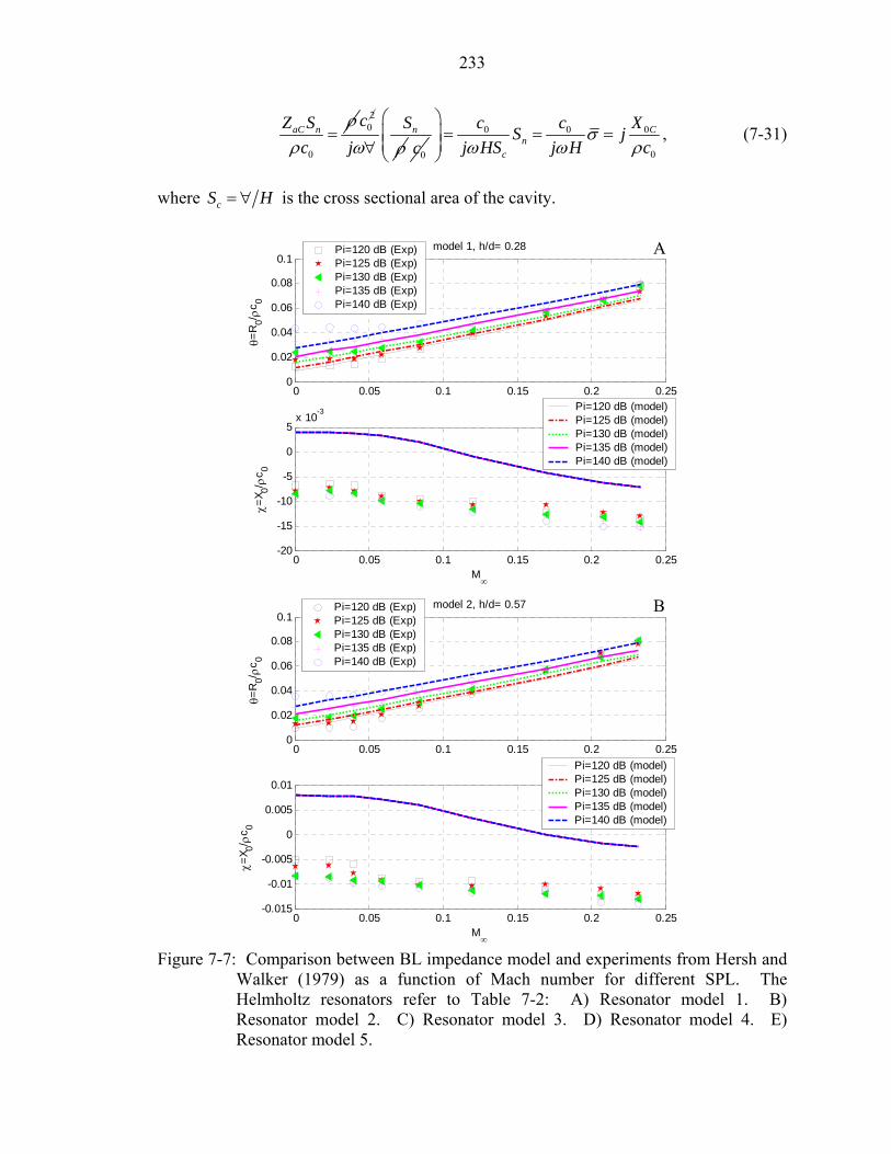
233

0

aC nZ Sc

ρρ

=2

0cnS

jω ρ∀ 0c0 0 0

0

Cn

c

c c XS jj HS j H c

σω ω ρ

⎛ ⎞= = =⎜ ⎟⎜ ⎟

⎝ ⎠, (7-31)

where cS H= ∀ is the cross sectional area of the cavity.

0 0.05 0.1 0.15 0.2 0.250

0.02

0.04

0.06

0.08

0.1θ=

R0/ ρ

c 0model 1, h/d= 0.28

0 0.05 0.1 0.15 0.2 0.25-20

-15

-10

-5

0

5x 10-3

M∞

χ=X 0/ ρ

c 0Pi=120 dB (Exp)Pi=125 dB (Exp)Pi=130 dB (Exp)Pi=135 dB (Exp)Pi=140 dB (Exp)

Pi=120 dB (model)Pi=125 dB (model)Pi=130 dB (model)Pi=135 dB (model)Pi=140 dB (model)

0 0.05 0.1 0.15 0.2 0.250

0.02

0.04

0.06

0.08

0.1

θ=R

0/ ρc 0

model 2, h/d= 0.57

0 0.05 0.1 0.15 0.2 0.25-0.015

-0.01

-0.005

0

0.005

0.01

M∞

χ=X 0/ ρ

c 0

Pi=120 dB (Exp)Pi=125 dB (Exp)Pi=130 dB (Exp)Pi=135 dB (Exp)Pi=140 dB (Exp)


Figure 7-7: Comparison between BL impedance model and experiments from Hersh and

Walker (1979) as a function of Mach number for different SPL. The Helmholtz resonators refer to Table 7-2: A) Resonator model 1. B) Resonator model 2. C) Resonator model 3. D) Resonator model 4. E) Resonator model 5.

B

A

234

0 0.05 0.1 0.15 0.2 0.250

0.02

0.04

0.06

0.08

0.1

θ=R

0/ ρc 0

model 3, h/d= 1.14

0 0.05 0.1 0.15 0.2 0.25-20

-15

-10

-5

0

5x 10-3

M∞

χ=X 0/ ρ

c 0

Pi=120 dB (Exp)Pi=125 dB (Exp)Pi=130 dB (Exp)Pi=135 dB (Exp)

Pi=120 dB (model)Pi=125 dB (model)Pi=130 dB (model)Pi=135 dB (model)

0 0.05 0.1 0.15 0.2 0.250

0.02

0.04

0.06

0.08

0.1

θ=R

0/ ρc 0

model 4, h/d= 2.28

0 0.05 0.1 0.15 0.2 0.25-10

-5

0

5x 10-3

M∞

χ=X 0/ ρ

c 0

Pi=115 dB (Exp)Pi=120 dB (Exp)Pi=125 dB (Exp)Pi=130 dB (Exp)

Pi=115 dB (model)Pi=120 dB (model)Pi=125 dB (model)Pi=130 dB (model)


C

D

235

0 0.05 0.1 0.15 0.2 0.250

0.02

0.04

0.06

0.08

0.1

θ=R

0/ ρc 0

model 5, h/d= 4.56

0 0.05 0.1 0.15 0.2 0.25-0.015

-0.01

-0.005

0

0.005

0.01

M∞

χ=X 0/ ρ

c 0

Pi=115 dB (Exp)Pi=120 dB (Exp)Pi=125 dB (Exp)Pi=130 dB (Exp)Pi=135 dB (Exp)



Clearly, the resistance is well captured, although the experimental data suggest a

nonlinear increase with the grazing flow Mach number. The resistance tends to not vary

for very low Mach numbers but increases after a threshold in the Mach number is

reached, and this is true for all models with different orifice aspect ratio h d . It also

appears that the effect of the incident pressure is primarily felt for low Mach numbers and

tends to saturate for higher values.

With regards to the reactance, the data are consistently overpredicted by the model

and start in the positive axis for the no flow condition, but the trend of a nearly constant

value with a slight decrease for higher Mach numbers is well captured. Also, the

reactance model is insensitive to the incident pressure amplitude. Note that although no

information was provided in Hersh and Walker (1979) about the grazing flow boundary

layer for the different Mach number tested, it was assumed that the boundary layer

thickness was held constant from the nominal case such that 7.62mmδ = for all tests.

E

236

Another suitable experimental dataset is that of Jing et al. (2001). Their set up is

shown in Figure 7-8, and Table 7-3 summarizes the test conditions and device geometry.

A grazing flow of Mach number varying from 0 to 0.15 was introduced through a square-

section wind tunnel of internal width 120.0 mm. A boundary layer survey was performed

using a Pitot-static tube and they show that the profile agrees with the well-known one-

seventh order power law for a turbulent boundary layer. The amplitudes of the sound

pressures measured by the two microphone method and their phase difference were then

utilized to compute the acoustic impedance of the tested sample in a similar manner as

presented above.

Table 7-3: Experimental operating conditions from Jing et al. (2001). ( )d mm ( )h mm ( )cD mm ( )H mm ( )%σ ( )f Hz ( )mmδ

3 2 32 150 2.94 200 30

Flowperforated plate

cylindricalcavity

microphones

A/Dcomputer

noisesource

Pitot-statictube

35mm

30 mm

150 mm

Figure 7-8: Experimental setup used in Jing et al. (2001). (Arranged from Jing et al. 2001)

237

0 0.02 0.04 0.06 0.08 0.1 0.12 0.14 0.16-0.02

-0.01

0

0.01

0.02

0.03

0.04

0.05

0.06

0.07

M∞

Z 0/ ρc 0

h/d= 0.66

Re(Z0/ρc0) ExperimentRe(Z0/ρc0) modelIm(Z0/ρc0) ExperimentIm(Z0/ρc0) model

Figure 7-9: Comparison between model and experiments from Jing et al. (2001). The

resonator design refers to Table 7-3.

Figure 7-9 compares the present model with the experimental data from Jing et al.

(2001), where the normalized impedance is plotted as a function of the grazing flow

Mach number. As in the previous example, the resistance model agrees with the

experimental data for low Mach numbers, while the overall reactance trend is captured as

well (nearly constant value as the Mach number increases). However, the resistance data

do not follow the same trend as in the previous example, since no plateau in the

resistance curve is observed in the low Mach number region for the data from Jing et al.

(2001).

It should be pointed out, however, that all these experimental data should be

regarded with some skepticism. They rely on the two microphone impedance technique

(Dean 1974) and no uncertainty estimates are provided. Also, good reactance data are

more difficult to obtain than resistance data, since the method principally relies on the

phase difference knowledge which, for instance, can be systematically altered by

238

instrumentation equipment data acquisition hardware and hydrodynamic effects in the

cavity. Also, the data were usually acquired when the device was operating near

resonance, when the radiated sound pattern can clearly extend to several orifice diameters

away from the resonator (typically, at resonance a Helmholtz resonator scattering cross

sectional area scales with the wavelength squared), hence resulting in a different acoustic

mass near the orifice exit. Proper placement of the microphone near the orifice is

therefore of great importance in order to retrieve the correct mass due to the end

correction. As generally concluded by the acoustic liner community, more accurate

calculations of the variation of the resonator resistance and reactance could only be made

if more flow details in the vicinity of the orifice are known.

Nevertheless, it should be emphasized that the goal of this exercise was not to

validate the grazing flow impedance model via available experimental data, since at the

present time no one has been able to accomplish this goal. The validation of low-order

models for flow past Helmholtz resonators is not the focus of this research. However, the

above discussion improves our understanding of the BL impedance model in its present

form and gives us some confidence in its use, while keeping in mind its limitations and

shortcomings.

Boundary layer impedance implementation in ZNMF actuator

In order to fully appreciate the effect of the key parameters present in the BL

impedance model, such as the Mach number M∞ , the boundary layer thickness to orifice

length ratio dδ , or kd , on the frequency response of a ZNMF actuator, the synthetic jet

design used in the NASA Langley workshop (CFDVal 2004) and denoted as Case 1 is

modeled and employed. In a similar way, the actuator designed by Gallas et al. (2003a)

239

and referred therein as Case 1 is also used, since the two resonant peaks that characterize

their dynamic behavior are reversed. In particular, in Case 1 (CFDVal 2004) the first

peak is due to the natural frequency of the diaphragm while the second one is governed

by the Helmholtz frequency of the resonator, while the opposite is true in Case 1 from

Gallas et al. (2003a). The first peak is dictated by the Helmholtz frequency while the

second peak corresponds to the piezoelectric-diaphragm natural frequency. The reader is

referred to the discussion in Chapter 5 on the cavity compressibility effect, where a

similar comparison between these two cases has already been performed; this discussion

gives a clear definition of the different governing frequencies of the system and their

respective effects.

0 500 1000 1500 2000 2500 30000

0.1

0.2

0.3

0.4

0.5

0.6

0.7

0.8

0.9

1

Frequency [Hz]

VC

L(LE

M) /

VC

L(exp

)

M∞

= 0

M∞

= 0.05

M∞

= 0.1

M∞

= 0.2

M∞

= 0.3

d = 1.27 mmδBL

= 10 mm

M∞

Figure 7-10: Effect of the freestream Mach number on the frequency response of the

ZNMF design from Case 1 (CFDVal 2004) using the refined LEM. The centerline velocity is normalized by the experimental data at the actuation frequency.

240

0 500 1000 1500 2000 2500 30000

5

10

15

20

25

30

35

40

45

50

Frequency [Hz]

Cen

terli

ne V

eloc

ity [m

/s]

M∞

= 0

M∞

= 0.05

M∞

= 0.1

M∞

= 0.2

M∞

= 0.3

d = 1.65 mmδBL

= 10 mm

M∞

Figure 7-11: Effect of the freestream Mach number on the frequency response of the

ZNMF design from Case 1 (Gallas et al. 2003a).

Figure 7-10 shows the effect of varying the freestream Mach number M∞ on the

centerline velocity of the actuator versus frequency for the Case 1 (CFDVal 2004) design,

while Figure 7-11 is for the Case 1 (Gallas et al. 2003a) design. The incoming grazing

flow is assumed to be characterized by a boundary layer 10mmδ = and a freestream

Mach number ranging from 0 to 0.3.

Clearly, the effect of the freestream Mach number is principally experienced at the

Helmholtz frequency peak, while a global decrease in magnitude is still seen over the

entire frequency range due to the increase in the total orifice resistance. Recalling the

definition of the Helmholtz frequency, Eqs. B-1 and B-2, the shift in frequency of the

peak is explained by the modification of the acoustic mass by the boundary layer or, more

specifically, by the decrease of the effective orifice length 0h . Since aBLM and aOM are

weak functions of the grazing flow parameters (only M∞ ), the Helmholtz frequency that

strongly depends of the acoustic masses in the system will therefore be only slightly

241

affected by the external BL. Hence, the cavity compressibility criterion described in

Chapter 5 should not be greatly affected and can be generalized to a ZNMF actuator with

an external boundary layer. Also, letting the ratio dδ vary will affect the overall

magnitude of the device response since it is present in the acoustic BL resistance

expression, although it will not affect the location of the frequency peaks since the

acoustic BL mass expression does not contain the ratio dδ .

Velocity Profile Scaling Laws

Despite the power of LEM that resides in its simplicity and reasonable estimate

(typically within 20%± ) achieved with minimal effort, it unfortunately does not provide

any information on the profile or shape of the jet exit velocity which is also strongly

phase dependant as seen in Chapter 4. In this regard, a low-dimensional model or

description of the jet velocity shape is needed, i.e. a parameterization of the profile in

terms of the key parameters that capture the important dynamic and kinematic features of

the orifice flow, as well as scaling laws that relate these parameters to the other flow

variables. In the first section of this chapter, it is proposed that the successive moments

and skewness of the jet velocity profile can be useful in characterizing ZNMF actuators.

However, dimensional analysis revealed a large parameter space (see Eq. 7-8). To be

applicable, some restrictions need to be employed since a candidate jet profile should be

low dimensional and also capable of reasonably matching the observed and measured jet

profile characteristics. Therefore, as a first step, a Blasius boundary layer is assumed to

characterize the incoming grazing flow that reduces the parameter space to

12

12

3, , , , , ,Re ,n

H d

C h wfn Sd d d dX

φθ

φ

ω ω θω ω

⎫ ⎛ ⎞∆∀⎪ =⎬ ⎜ ⎟⎝ ⎠⎪⎭

. (7-32)

242

Two approaches are described next that yield two different scaling laws of a ZNMF

actuator issuing into a grazing boundary layer. One focuses on fitting the velocity profile

( ),v x t at the actuator exit, while the other one employs a model based on the local

integral parameters of the actuator, such as the successive moments 12

nCφ and skewness

12Xφ , as shown in Figure 7-12.

Table 7-4: Tests cases from numerical simulations used in the development of the velocity profiles scaling laws

Case h d dθ S Re j Reθ jV U∞ W d H d 0W d

I 1 0.266 20 188 133 0.375 3 1.5 0.393 II 1 0.266 20 281 133 0.563 3 1.5 0.393 III 1 0.266 20 375 133 0.75 3 1.5 0.393 IV 1 0.133 20 188 133 0.188 3 1.5 0.393 V 1 0.399 20 62 133 0.188 3 1.5 0.393 VI 1 0.532 20 47 133 0.188 3 1.5 0.393 VII 1 0.266 20 24 33 0.188 3 1.5 0.393 VIII 1 0.266 20 47 66 0.188 3 1.5 0.393 IX 1 0.266 20 188 266 0.188 3 1.5 0.393 X 1 0.266 5 94 133 0.188 3 1.5 0.393 XI 1 0.266 10 94 133 0.188 3 1.5 0.393

XII* 1 0.266 20 94 133 0.188 4 1.5 0.393 XIII 1 0.266 50 94 133 0.188 3 1.5 0.393

* Nominal / Test case

To develop these scaling laws, numerical simulations from the George Washington

University, courtesy of Prof. Mittal, are again used in a joint effort. The 2D numerical

simulations described in Appendix F are employed to construct the test matrix given in

Table 7-4. It consists of 13 cases, all based on a nominal flow condition (Case XII), 4

flow parameters being systematically varied around the nominal case. In Cases I to III,

the ratio jV U∞ is varied from about 0.2 to 0.75. Case IV to Case VI vary dθ , whereas

243

in Cases VII to IX the jet Reynolds number is varied. Finally the Stokes number is varied

in Cases X to XIII.

The velocity profile scaling laws are next detailed. For both approaches, the idea is

to first assume a candidate jet velocity profile and, based on the test matrix comprised of

CFD simulation results (summarized in Table 7-4), the candidate jet velocity profile is

refined, and a regression analysis is then performed to yield a scaling law that predicts

either the velocity profile or the integral parameters as a function of the main

dimensionless numbers. The candidate profile is adapted from Rampuggoon (2001) who

performed a similar study on modeling the velocity profile of ZNMF actuator exhausting

in an external crossflow (his motivation was to try to match the integral parameters of his

test cases). He assumed a candidate velocity profile of the form

( ) ( ) ( ), sinj x t T x tω=V , (7-33)

where 2x x d= is the normalized spatial coordinate across the orifice. However, his

chosen profile ( )T x was just a parabolic-type profile of steady channel flow. Here, this

work is extended to a more general approach, where the choice of ( )T x is motivated by

the results of the investigation outlined in Chapter 4 on the 2D slot flow physics of a

ZNMF actuator in a quiescent medium. It takes the form

( )( )( )

cosh 21

cosh 2

x S jT x

S j

⎧ ⎫−⎪ ⎪= −⎨ ⎬−⎪ ⎪⎩ ⎭

, (7-34)

which satisfies the no-slip condition at the orifice walls and is already Stokes-number

dependant in accordance with pressure-driven oscillatory flow in a channel (White 1991).

Each scaling law is now detailed.

244

( ) ( ) ( )( ), sinx t T x t T xω= ⋅ +∠V

Figure 7-12: jet

Scaling law b

This ap

exit, as a fun

summarized in

In the f

since the velo

component –

such that

Then, b

magnitude, an

squares curve

for each comp

Jet exit scaling laws based on
Match the velocityprofile
Schematic of the two approaches used to exit velocity profile.

ased on the jet exit velocity profile

proach focuses on the shape of the velo

ction of the phase angle. The methodo

Figure 7-13 and is comprised of 5 steps.

irst step, a candidate velocity profile is

city profile is sinusoidal in nature, it ca

equivalent to an average – plus a magnit

( ) ( ) ( ), sindecomp dc magx t x x= + ⋅V V V

ased on the candidate jet velocity profil

d phase angle are extracted from the C

fit is performed to yield a corrected can

onent.

( ),x tV

Match the integral parameters

develop the scaling laws from the

city profile at the actuator orifice

logy to develop a scaling law is

chosen, as detailed above. Next,

n be simply decomposed by a dc

ude and phase angle components,

( )( )argt xω + V . (7-35)

e ( ),T x t , the local average (dc),

FD results, and a nonlinear least-

didate velocity profile, ( )mod ,T x t

3, , , ,vC X Cµ Ω …

245

( ) ( )( )

cosh 21

cosh 2

x S jT x

S j

−= −

−

( ) ( )arg, sindecomp dc magx t tω= + +V V V V

( )

arg

find , , such that

find , such that

find , , such that sin

cxmag

hxdc

a b c T a be

d e T dx e

g h i i gx e

⎧ = +⎪⎪ −∠ = +⎨⎪

=⎪⎩

V

V

V

( )mod mod, mod, mod,argsindc magT T t Tω= + +V

mod,cx

magT T a be= +

mod,argT T dx e= ∠ + +

( ) mod, sin hxdcT i gx e=

( ) ( ) ( ) ( )

41 2 3

00 0 0 0

, ,Re, ,Re

, ,

bb b b

j

j

a b cV Uh d dd e a

h d d V Ug h i

θ

θ

θθ

∞

∞

⎧ ⎫ ⎡ ⎤⎡ ⎤ ⎡ ⎤ ⎡ ⎤⎪ ⎪ ⎢ ⎥= ⋅ ⋅ ⋅ ⋅⎢ ⎥ ⎢ ⎥ ⎢ ⎥⎨ ⎬ ⎢ ⎥⎢ ⎥ ⎢ ⎥ ⎢ ⎥⎪ ⎪ ⎣ ⎦ ⎣ ⎦ ⎣ ⎦ ⎣ ⎦⎩ ⎭

Figure 7-13: Methodology for the development of the velocity profile based scaling law.

Candidate velocity profile

Decompose CFD velocity profile

Fit low-order models for each components via nonlinear least square curve fits

Nonlinear regression analysis to obtain an empirical scaling

law of the form:

246

The results are shown in Figure 7-14, Figure 7-15, Figure 7-16, Figure 7-17, Figure

7-18, Figure 7-19, and Figure 7-20 for Case I, Case III, Case V, Case VII, Case IX, Case

XI, and Case XIII, respectively; Table 7-5 summarizes the value that all 8 coefficients

take for each test case. For each figure, the comparison between the candidate velocity

profile ( ),T x t , decomposed into its magnitude T and argument T∠ , is compared with

the equivalent model ( mod,magT and mod,argT , respectively) and the CFD data. The choice of

the three models, namely

( )

mod,

mod,arg

mod, sin

cxmag

hxdc

T T a be

T T dx e

T i gx e

⎧ = +⎪⎪ = ∠ + +⎨⎪

=⎪⎩

(7-36)

is motivated so that it yields the “best fit” for all cases studied. For instance, the ratio of

the amplitudes, mag TV , has usually large gradients near the edge of the orifice but

remains quite “flat” in the center. Similarly, it is found that the phase difference

arg T−∠V varies linearly over the slot depth. Finally, notice that the dc value of the

decomposed velocity profile, which can be thought of as the velocity average across the

orifice, is usually an order of magnitude less than the amplitude value and has a

sinusoidal-type shape. Although not perfect, the modeled profiles are in agreement with

the CFD data.

247

0.1

0.15

model = i.sin(gx).ehx

CFDTmod

Figu

-1 -0.5 0 0.5 10.5

1

1.5

2

x/(d/2)

ampl

itude

ratio model = a + becx

-1 -0.5 0 0.5 10

0.5

1

1.5

ampl

itude

T Tmod CFD

-1 -0.5 0 0.5 1-50

0

50

x/(d/2)

phas

e di

ff (d

eg)

model = dx+e

-1 -0.5 0 0.5 1-50

0

50

100

phas

e (d

eg) T

TmodCFD

Re 188=⎧

A B

-1 -0.5 0 0.5 1-0.1

-0.05

0

0.05

x/(d/2)

aver

age

re 7-14: Nonlinear least square curve fit on the decomposed jet velocity profile for Case I. A) Amplitude. B) Phase angle. C) dc components. The blue curves are for the components of the candidate profile ( ),T x t ; the green curves are

for the components of the modeled profile ( )mod ,T x t ; the red curves are the CFD results.

Re 13320S

θ⎪ =⎨⎪ =⎩

C

248

0.05

0.1

0.15model = i.sin(gx).ehx

Figu

-1 -0.5 0 0.5 10.5

1

1.5

2

x/(d/2)

ampl

itude


-1 -0.5 0 0.5 10

0.5

1

1.5

ampl

itude

TTmodCFD

-1 -0.5 0 0.5 1-50

0

50

x/(d/2)

phas

e di

ff (d

eg)

model = dx+e

-1 -0.5 0 0.5 1-50

0

50

100

phas

e (d

eg) T

TmodCFD

Re 375=⎧

A B

-1 -0.5 0 0.5 1-0.2

-0.15

-0.1

-0.05

0

x/(d/2)

aver

age

CFDTmod

re 7-15: Nonlinear least square curve fit on the decomposed jet velocity profile for Case III. A) Amplitude. B) Phase angle. C) dc components. The blue curves are for the components of the candidate profile ( ),T x t ; the green curves are


Re 13320S

θ⎪ =⎨⎪ =⎩

C

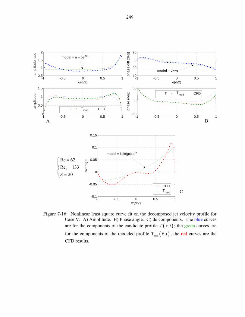
249

0.05

0.1

0.15

e


Figure

-1 -0.5 0 0.5 10.5

1

1.5

2

x/(d/2)

ampl

itude


-1 -0.5 0 0.5 10

0.5

1

1.5

ampl

itude

T Tmod CFD

-1 -0.5 0 0.5 1-40

-20

0

20

x/(d/2)

phas

e di

ff (d

eg)

model = dx+e

-1 -0.5 0 0.5 1-50

0

50

phas

e (d

eg) T Tmod CFD

Re 62=⎧

A B

-1 -0.5 0 0.5 1-0.1

-0.05

0

x/(d/2)

aver

ag

CFDTmod

7-16: Nonlinear least square curve fit on the decomposed jet velocity profile for Case V. A) Amplitude. B) Phase angle. C) dc components. The blue curves are for the components of the candidate profile ( ),T x t ; the green curves are


Re 13320S

θ⎪ =⎨⎪ =⎩

C

250

0.02

0.04

0.06CFDTmod

Figure

-1 -0.5 0 0.5 10.5

1

1.5

2

x/(d/2)

ampl

itude


-1 -0.5 0 0.5 10

0.5

1

1.5

ampl

itude

T Tmod CFD

-1 -0.5 0 0.5 1-20

-10

0

10

x/(d/2)

phas

e di

ff (d

eg)

model = dx+e

-1 -0.5 0 0.5 1-50

0

50

phas

e (d

eg)

T Tmod CFD

Re 24=⎧

A B

-1 -0.5 0 0.5 1-0.06

-0.04

-0.02

0

x/(d/2)

aver

age


7-17: Nonlinear least square curve fit on the decomposed jet velocity profile for Case VII. A) Amplitude. B) Phase angle. C) dc components. The blue curves are for the components of the candidate profile ( ),T x t ; the green

curves are for the components of the modeled profile ( )mod ,T x t ; the red curves are the CFD results.

C

Re 3320S

θ⎪ =⎨⎪ =⎩

251

0.05

0.1

0.15

e


CFDTmod

Fi

-1 -0.5 0 0.5 10

1

2

3

x/(d/2)

ampl

itude


-1 -0.5 0 0.5 10

1

2

ampl

itude

T Tmod CFD

-1 -0.5 0 0.5 1-100

-50

0

50

x/(d/2)

phas

e di

ff (d

eg)

model = dx+e

-1 -0.5 0 0.5 1-50

0

50

100

phas

e (d

eg) T

TmodCFD

Re 188=⎧

B A

-1 -0.5 0 0.5 1-0.1

-0.05

0

x/(d/2)

aver

ag

gure 7-18: Nonlinear least square curve fit on the decomposed jet velocity profile for Case IX. A) Amplitude. B) Phase angle. C) dc components. The blue curves are for the components of the candidate profile ( ),T x t ; the green curves are


Re 26620S

θ⎪ =⎨⎪ =⎩

C

252

0.05

0.1

e


Figure

-1 -0.5 0 0.5 10

2

4

6

x/(d/2)

ampl

itude

ratio

model = a + becx

-1 -0.5 0 0.5 10

1

2

ampl

itude

T Tmod CFD

-1 -0.5 0 0.5 1-100

-50

0

50

x/(d/2)

phas

e di

ff (d

eg)

model = dx+e

-1 -0.5 0 0.5 1-50

0

50

100

phas

e (d

eg) T Tmod CFD

Re 94=⎧

A

B

-1 -0.5 0 0.5 1-0.1

-0.05

0

x/(d/2)

aver

ag

CFDTmod

7-19: Nonlinear least square curve fit on the decomposed jet velocity profile for Case XI. A) Amplitude. B) Phase angle. C) dc components. The blue curves are for the components of the candidate profile ( ),T x t ; the green curves are


C

Re 13310S

θ⎪ =⎨⎪ =⎩

253

0

0.2

0.4

e

CFDTmod

Fi

-1 -0.5 0 0.5 10.5

1

1.5

2

x/(d/2)

ampl

itude


-1 -0.5 0 0.5 10

0.5

1

1.5

ampl

itude

T Tmod CFD

-1 -0.5 0 0.5 1-20

-10

0

10

x/(d/2)

phas

e di

ff (d

eg)

model = dx+e

-1 -0.5 0 0.5 1-20

0

20

40

phas

e (d

eg) T

TmodCFD

Re 94=⎧

A B

-1 -0.5 0 0.5 1-0.6

-0.4

-0.2

x/(d/2)

aver

ag


gure 7-20: Nonlinear least square curve fit on the decomposed jet velocity profile for Case XIII. A) Amplitude. B) Phase angle. C) dc components. The blue curves are for the components of the candidate profile ( ),T x t ; the green

curves are for the components of the modeled profile ( )mod ,T x t ; the red curves are the CFD results.

C

Re 13350S

θ⎪ =⎨⎪ =⎩

254

Table 7-5: Coefficients of the nonlinear least square fits on the decomposed jet velocity profile

Case a b c d e g h i I 2.46 -1.45 0.11 -27.57 -5.18 -3.15 7.29 -5.10-5 II 2.71 -1.66 0.13 -25.97 -11.82 -1.29 -1.28 -0.05 III 0.56 0.34 1.09 -28.13 -10.44 -2.82 -0.37 -0.08 IV 0.38 1.33 0.52 -59.83 6.71 -3.12 0.22 0.11 V 0.91 0.002 6.48 -12.91 -6.49 -0.43 0.49 -0.15 VI 0.90 0.003 5.67 -6.70 -6.42 4.89 1.39 -0.02 VII 0.89 0.003 5.69 -6.82 -7.08 -12.56 5.18 5.10-5 VIII 0.90 0.002 6.01 -13.02 -5.63 -3.12 10.78 -2.10-5 IX 0.81 0.01 5.40 -43.95 -5.03 -3.49 -0.40 0.084 X 0.68 0.01 6.80 -13.06 -23.61 -1.61 -0.16 -0.05 XI 0.70 0.02 5.81 -41.91 -3.32 -0.61 -0.311 -0.09 XII 0.93 0.002 6.09 -33.17 -5.69 -0.32 1.34 -0.18 XIII 0.85 0.006 4.82 -0.07 -8.69 -2.65 0.89 0.24

Next, the 4th step shown in Figure 7-13 consists of recombining each component of

the modeled profile developed above, such that the final modeled velocity profile takes

the form

( ) ( ) ( ) ( )( )mod mod, mod, mod,arg, sindc magx t T x T x t T xω= + ⋅ +V , (7-37)

and is a function of the 8 parameters , , , , , , ,a b c d e g h i . Notice that Eq. 7-37 is time and

spatial dependant and that it needs at least these 8 parameters to represent it. Figure 7-21

compares the velocity profiles at the orifice exit from the CFD results, the decomposition

of the velocity decompV defined in Eq. 7-35, and the modeled velocity profile modV defined

by Eq. 7-37. First of all, it can be seen that the velocity profile decomposition in terms of

a dc term plus a sinusoidal time variation is a good approximation of the velocity profile

at the orifice exit from the CFD results for all cases studied. Similarly, following the

discussion above, the overall modeled profiles tend to be in agreement with the CFD

data, and again at each instant in time during a cycle (although only four phase angles

have been shown in Figure 7-21 for clarity). Clearly, the choice of the candidate velocity

255

profile that is Stokes number dependent is able to capture the Richardson effect

(overshoot near the orifice edge) that is present in all cases. Notice also how different

can the velocity profiles be among the test cases considered, and still this 8-parameters

candidate velocity profile model is capable of representing a large variety of velocity

profiles, some being completely skewed, others nearly symmetric. Thus, based on this

finding, the nest step in developing a scaling law can be taken and is described next.

Figure 7-21: Comparison between CFD velocity profile, decomposed jet velocity profile, and modeled velocity profile, at the orifice exit, for four phase angles during a cycle. A) Case I. B) Case II. C) Case III. D) Case IV. E) Case V. F) Case VI. G) Case VII. H) Case VIII. I) Case IX. J) Case X. K) Case XI. L) Case XIII. The velocity in the vertical abscise is normalized by U∞ .

-1 -0.5 0 0.5 1-1.5

-1

-0.5

0

0.5

1

1.5

2x/d

CFD Vdecomp Vmod

φ = 0°

φ = 92°

φ = 229°

φ = 266°

-1 -0.5 0 0.5 1-1.5

-1

-0.5

0

0.5

1

1.5

2x/d

CFD Vdecomp Vmod

φ = 0°

φ = 92°

φ = 229°

φ = 266°A B

256


-1 -0.5 0 0.5 1-1.5

-1

-0.5

0

0.5

1

1.5

2x/d

CFD Vdecomp Vmod

φ = 0°

φ = 92°

φ = 229°

φ = 266°

-1 -0.5 0 0.5 1-1.5

-1

-0.5

0

0.5

1

1.5

2x/d

CFD Vdecomp Vmod

φ = 0°

φ = 92°

φ = 229°

φ = 266°G H

-1 -0.5 0 0.5 1-1.5

-1

-0.5

0

0.5

1

1.5

2x/d

CFD Vdecomp Vmod

φ = 0°

φ = 92°

φ = 229°

φ = 266°

-1 -0.5 0 0.5 1-1.5

-1

-0.5

0

0.5

1

1.5

2x/d

CFD Vdecomp Vmod

φ = 0°

φ = 92°

φ = 229°

φ = 266°E F

-1 -0.5 0 0.5 1-2

-1.5

-1

-0.5

0

0.5

1

1.5

2x/d

CFD Vdecomp Vmod

φ = 0°

φ = 92°

φ = 229°

φ = 266°

-1 -0.5 0 0.5 1-1.5

-1

-0.5

0

0.5

1

1.5

2x/d

CFD Vdecomp Vmod

φ = 0°

φ = 92°

φ = 229°

φ = 266°C D

257


As shown in Figure 7-13, the next logical step is to extract a scaling law relating

the computed values of the parameters , , , , , , ,a b c d e g h i to the dimensionless flow

parameters. Because the relationship among the involved parameters and the target

values, i.e. the family set , , , , , , ,a b c d e g h i , is nonlinear as can be seen by inspection, a

nonlinear regression technique is sought for deriving an empirical scaling law, which can

be implemented in any available commercial statistical calculation software such as SPSS

-1 -0.5 0 0.5 1-2

-1.5

-1

-0.5

0

0.5

1

1.5

2x/d

CFD Vdecomp Vmod

φ = 0°

φ = 92°

φ = 229°φ = 266°

-1 -0.5 0 0.5 1-2

-1.5

-1

-0.5

0

0.5

1

1.5

2

2x/d

CFD Vdecomp Vmod

φ = 0°

φ = 92°

φ = 229°

φ = 266°K L

-1 -0.5 0 0.5 1-2

-1.5

-1

-0.5

0

0.5

1

1.5

2

2x/d

CFD Vdecomp Vmod

φ = 0°

φ = 92°

φ = 229°

φ = 266°

-1 -0.5 0 0.5 1-2

-1.5

-1

-0.5

0

0.5

1

1.5

2

2x/d

CFD Vdecomp Vmod

φ = 0°

φ = 92°

φ = 229°

φ = 266°

I J

258

(Statistical Analysis System). Taking into account the effect of the most important

parameters, such as the orifice aspect ratio h d , the Stokes number S (already present in

the functional form of the velocity profile), the BL momentum thickness to orifice

diameter dθ , the BL Reynolds number Reθ and the nominal jet-to-freestream velocity

ratio jV U∞ , an empirical scaling law for the 8 coefficients of the modeled velocity

profile in Eq. 7-37 can be obtained by the regression analysis. The chosen target function

takes the general form

( ) ( ) ( ) ( )

41 2 3

00 0 0 0

, ,Re, ,Re

, ,

bb b b

j

j

a b cV Uh d dd e a

h d d V Ug h i

θ

θ

θθ

∞

∞

⎧ ⎫ ⎡ ⎤⎡ ⎤ ⎡ ⎤ ⎡ ⎤⎪ ⎪ ⎢ ⎥= ⋅ ⋅ ⋅ ⋅⎢ ⎥ ⎢ ⎥ ⎢ ⎥⎨ ⎬ ⎢ ⎥⎢ ⎥ ⎢ ⎥ ⎢ ⎥⎪ ⎪ ⎣ ⎦ ⎣ ⎦ ⎣ ⎦ ⎣ ⎦⎩ ⎭

, (7-38)

where 0a and ib are the regression coefficients (with 1,2,3,4i = ). Here, 0a is the

respective “nominal” value of a, b, c, d, e, g, h, or i, while the b’s are the exponent of

each nondimensional term.

These regression coefficients are determined by the nonlinear regression analysis

with the data provided in Table 7-5, i.e. for 12 cases since the test case (Case XII) is left

out of this regression analysis for verification purposes. The results are given in Table

7-6 where R2 is the correlation coefficient. Before commenting on these results, it should

be pointed out that this problem is clearly over-parameterized, i.e., the family set contains

8 parameters for only 12 numerical cases to do the regression analysis. Therefore, the

next steps are explained only for illustration purposes.

259

Table 7-6: Results from the nonlinear regression analysis for the velocity profile based scaling law R2 a0 b1 b2 b3 b4

a 0.225 0.903 1.0 0.276 -0.0182 0.490b 0.102 -0.123 1.0 1.028 0.300 1.161c 0.786 4.983 1.0 0.533 -0.0969 -4.402d 0.730 -20.70 1.0 -1.526 1.046 0.238e 0.122 -6.182 1.0 0.668 -0.085 0.405g 0.163 0.010 1.0 -3.502 3.078 -11.02h 0.303 8 x10-10 1.0 32.43 -0.0375 -0.576i 0.267 1.772 1.0 0.087 -1.008 -0.329

First of all, notice the small correlation coefficients R2 for all parameters but c and

d, far from unity, indicative of the poor confidence level in the corresponding regression

coefficients. Clearly, such low correlation coefficients indicate a sub-optimal regression

form. One way to increase the R2 values is to increase the test matrix, by more covering

the parametric space used here. Keeping in mind the poor level of confidence in these

parameters, it is still worthwhile to examine the relative values of the coefficients a0 and

bi, a0 being representative of the importance of the parameter a to i. It can be seen from

the parameter a that the dc part of the profile (parameters g, h, and i) does not have a

significant influence on the overall profile, compared with d and e from the phase angle

or a, b and c from the magnitude. Next, the constant value for the coefficient b1 is due to

the fact that the ratio h d has not been varied in the test cases used in this analysis, as

shown in Table 7-4. Finally, at this stage it is quite difficult to draw firm conclusions

concerning the other coefficients b2, b3, and b4, with such low associated R2 values.

Nonetheless, for verification purposes the test case (Case XII) is used to evaluate

the velocity profile based scaling law. The results are shown in Figure 7-22 where the

numerical data are plotted along with the scaling law of the velocity profile obtained by

260

applying the results in Table 7-6 into the modeled profile defined in Eq. 7-37. Only four

phase angles 0; ;5 4;3 2π π π are plotted for clarity. Clearly, the proposed scaling law

fails to accurately predict the actual velocity profile. Although the velocity is in

agreement near the upstream edge of the orifice, it is clearly over-predicted near the

downstream orifice edge. This should mainly come from the functional form chosen for

the magnitude term mod,cx

magT T a be= + which has really poor associated regression

coefficients R2. Recall however that this all analysis has been performed on only 12

cases, which is a modest but valuable start in view of the results presented in this section.

It is clearly not enough if one considers the wide parameter space to span and the strongly

coupled interactions between each dimensionless parameter.

-1 -0.5 0 0.5 1-8

-6

-4

-2

0

2

4

6

8

2x/d

velo

city

(vj/U

∞)

CFDscaling law

φ = 0°φ = 92°

φ = 229°φ = 266°

Figure 7-22: Test case comparison between CFD data and the scaling law based on the

velocity profile at four phase angles during a cycle. Case XII: S = 20, Re = 94, 0.26dθ = , Re 133θ = .

261

Scaling law based on the jet exit integral parameters

The first scaling law previously presented is using the spatial velocity profile at the

orifice exit, but disregards the integral parameters (momentum coefficient, skewness,

vorticity flux,…). Another approach - presented next - is to base the scaling law on these

integral parameters, regardless of the actual velocity profile. The methodology of this

approach is outlined in Figure 7-23. First, a candidate velocity profile is chosen, in a

similar fashion as already explained above. Because of the zero-net mass flux nature of

the device, the dc or average component of the velocity should be identically zero in a

time average sense. Hence, the candidate profile is refined such that the new low-order

model for the velocity profile takes the form

( ) ( ) ( )( )mod arg, sinmagx t x t xω= ⋅ +V V V , (7-39)

where the magnitude and argument of the velocity are defined by

( ) ( ) ( )( ) ( ) ( )

2

arg

mag x ax bx c T x

x bx c T x

⎧ = + + ⋅⎪⎨

= + ⋅∠⎪⎩

V

V (7-40)

Notice that ( )mod ,x tV is a low-parameterized model since it is only function of 3

parameters: a, b, and c. Again, this functional form is motivated by the results of the

investigation outlined in Chapter 4 on the 2D slot flow physics of a ZNMF actuator in a

quiescent medium. But since only the integral parameters are of interest in here, the

shape of the velocity profile is not considered as crucial and thus does not have a more

complex functional form as seen in the previous scaling law.

262

( ) ( )( )

cosh 21

cosh 2

x S jT x

S j

−= −

−

( ) ( )( ) ( )

2

arg

mag ax bx c T x

bx c T x

⎧ = + +⎪⎨

= + ∠⎪⎩

V

V

( )mod argsinmag tω= +V V V

2 3, / , / / / /, , , ,j ex in ex in ex in ex in ex inC X Cµ ΩV

( ) ( )1 , ,mod , ,mod , ,

2 22 , / , mod , /

3 / ,mod /

4 / ,mod /

3 35 / ,mod /

0

000

0

j ex j in j ex j in

ex in ex in

ex in ex in

ex in ex in

ex in ex in

f

f C Cf X Xf

f C C

µ µ

⎧ = + − + =⎪⎪ = − =⎪⎪ = − =⎨⎪ = Ω −Ω =⎪⎪ = − =⎪⎩

V V V V

( ) ( ) ( ) ( )

41 2 3

00 0 0 0

Re, ,Re

bb b b

j

j

V Uh d da b c ah d d V U

θ

θ

θθ

∞

∞

⎡ ⎤⎡ ⎤ ⎡ ⎤ ⎡ ⎤⎢ ⎥= ⋅ ⋅ ⋅ ⋅⎢ ⎥ ⎢ ⎥ ⎢ ⎥⎢ ⎥⎢ ⎥ ⎢ ⎥ ⎢ ⎥⎣ ⎦ ⎣ ⎦ ⎣ ⎦ ⎣ ⎦

Figure 7-23: Methodology for the development of the integral parameters based scaling

law.

Nonlinear regression analysis to obtain an empirical scaling

law of the form:

Candidate velocity profile

Compute integral parameters from CFD simulations

find a, b, c such that

263

The requirements of this model profile are:

1. zero-net mass flux (identically satisfied by the assumed functional form)

2. match momentum coefficient

( )2 1 2

0 1

1 1 ,2 2

xC x d dd d

π

µ φ φπ θ −

⎛ ⎞= ⎜ ⎟

⎝ ⎠∫ ∫ V (7-41)

3. match skewness coefficient

( ) ( )2 1

0 0

1 , ,2 2

xX x x d dd

πφ φ φ

π⎛ ⎞

= − −⎡ ⎤ ⎜ ⎟⎣ ⎦⎝ ⎠

∫ ∫ V V (7-42)

4. match vorticity flux

( ) ( ) ( )2 1 2 2

0 1 0

1, , 0,2 2v

d xv x v x d d v ddx d

π πφ φ φ φ φ

−

⎛ ⎞⎛ ⎞Ω = − ⋅ =⎜ ⎟⎜ ⎟⎝ ⎠ ⎝ ⎠

∫ ∫ ∫ (7-43)

5. match jet kinetic energy flux

( )2 1 33

0 1

1 1 ,2 2

xC x d dd d

πφ φ

π θ −

⎛ ⎞= ⎜ ⎟

⎝ ⎠∫ ∫ V (7-44)

Recall that ( ) ( ), ,x v x Uφ φ ∞=V is the normalized velocity and that Eqs. 7-41,

7-42, 7-43, and 7-44 are derived for a 2D slot orifice geometry. Also, the vorticity flux

should be nondimensionalized with, for instance, the quantity jV d .

As outlined in Figure 7-23, the procedure is thus to compute these integral

parameters from the CFD data of the test cases tabulated in Table 7-4, and then to solve

for the coefficients a, b, and c from the modeled velocity profile (Eq. 7-39) to match

them. This yields a system of 5 equations and 3 unknowns to solve, that can be written as

264

( ) ( )1 , ,mod , ,mod , ,

2 22 , / ,mod , /

3 / ,mod /

4 , / ,mod , /

3 35 / ,mod /

0

0

find , , such that 00

0

j ex j in j ex j in

ex in ex in

ex in ex in

v ex in v ex in

ex in ex in

f

f C C

a b c f X Xf

f C C

µ µ

⎧ = + − + =⎪⎪ = − =⎪⎪ = − =⎨⎪ = Ω −Ω =⎪⎪ = − =⎪⎩

V V V V

(7-45)

Eq. 7-45 is clearly an over-determined system, with more equations than

unknowns. Recall also that the suffix ‘ex’ and ‘in’ stand for ‘expulsion’ and ‘ingestion’.

So one can actually compute the equations f2, f3, f4, or f5 for either the expulsion part or

the ingestion part of the cycle, which can add the number of equations up to 9.

Therefore, some choices have to be made to reduce the number of equations in Eq. 7-45

First of all, f1 can be removed since it insures the zero-net mass flux criterion, which is

automatically satisfied by the assumed functional form (Eqs. 7-39 and 7-40). Then, the

momentum flux can be recast to account for both the expulsion and ingestion parts, and

only the expulsion parts of the skewness coefficient and normalized vorticity flux are

retained. The new nonlinear system to be solved can then be written as

( ) ( )2 2 2 2

1 , ,mod , ,mod , ,

2 ,mod

3 , ,mod ,

0

find , , such that 0

0

ex in ex in

ex ex

v ex j v ex j

f C C C C

a b c f X X

f V d V d

µ µ µ µ⎧ = + − + =⎪⎪ = − =⎨⎪

= Ω −Ω =⎪⎩

. (7-46)

These 3 coefficients are numerically obtained via the Matlab function FSOLVE.

The results are summarized in Table 7-7 showing the results for the 3 parameters a, b,

and c, along with the corresponding equations f1, f2, and f3 from Eq. 7-46. Also, Table

7-8 shows the resulting integral parameters computed from the CFD data and the low-

order model. Clearly, the candidate velocity profile is able to accurately predict the

integral parameters when compared with the CFD data for the expulsion and ingestion

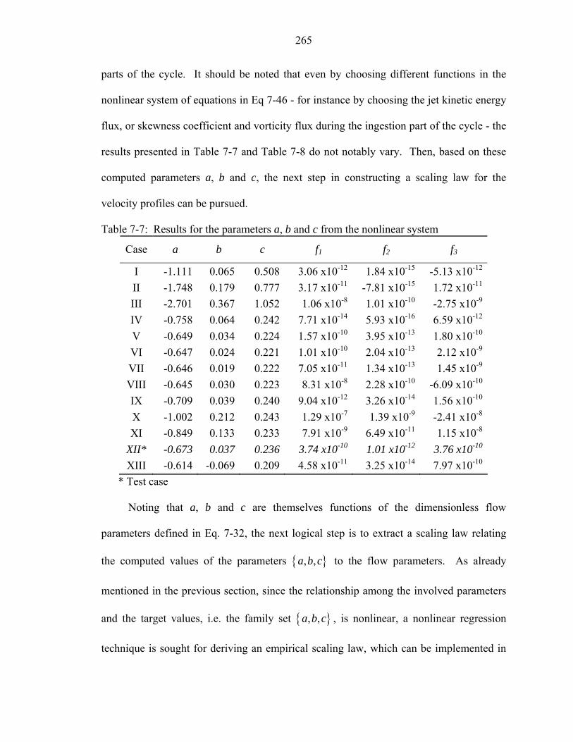
265

parts of the cycle. It should be noted that even by choosing different functions in the

nonlinear system of equations in Eq 7-46 - for instance by choosing the jet kinetic energy

flux, or skewness coefficient and vorticity flux during the ingestion part of the cycle - the

results presented in Table 7-7 and Table 7-8 do not notably vary. Then, based on these

computed parameters a, b and c, the next step in constructing a scaling law for the

velocity profiles can be pursued.

Table 7-7: Results for the parameters a, b and c from the nonlinear system

Case a b c f1 f2 f3

I -1.111 0.065 0.508 3.06 x10-12 1.84 x10-15 -5.13 x10-12

II -1.748 0.179 0.777 3.17 x10-11 -7.81 x10-15 1.72 x10-11

III -2.701 0.367 1.052 1.06 x10-8 1.01 x10-10 -2.75 x10-9

IV -0.758 0.064 0.242 7.71 x10-14 5.93 x10-16 6.59 x10-12

V -0.649 0.034 0.224 1.57 x10-10 3.95 x10-13 1.80 x10-10

VI -0.647 0.024 0.221 1.01 x10-10 2.04 x10-13 2.12 x10-9

VII -0.646 0.019 0.222 7.05 x10-11 1.34 x10-13 1.45 x10-9

VIII -0.645 0.030 0.223 8.31 x10-8 2.28 x10-10 -6.09 x10-10

IX -0.709 0.039 0.240 9.04 x10-12 3.26 x10-14 1.56 x10-10

X -1.002 0.212 0.243 1.29 x10-7 1.39 x10-9 -2.41 x10-8

XI -0.849 0.133 0.233 7.91 x10-9 6.49 x10-11 1.15 x10-8

XII* -0.673 0.037 0.236 3.74 x10-10 1.01 x10-12 3.76 x10-10

XIII -0.614 -0.069 0.209 4.58 x10-11 3.25 x10-14 7.97 x10-10

* Test case

Noting that a, b and c are themselves functions of the dimensionless flow

parameters defined in Eq. 7-32, the next logical step is to extract a scaling law relating

the computed values of the parameters , ,a b c to the flow parameters. As already

mentioned in the previous section, since the relationship among the involved parameters

and the target values, i.e. the family set , ,a b c , is nonlinear, a nonlinear regression

technique is sought for deriving an empirical scaling law, which can be implemented in

266

any available commercial statistical calculation software such as SPSS (Statistical

Analysis System).

Table 7-8: Integral parameters results Cµ ,modCµ X modX Case

ex in ex in ex in ex in I 0.114 0.106 0.110 0.110 0.017 -0.008 0.017 -0.017 II 0.281 0.258 0.257 0.282 0.069 -0.031 0.069 -0.076 III 0.662 0.441 0.538 0.565 0.171 -0.069 0.171 -0.179 IV 0.037 0.034 0.037 0.035 0.027 -0.061 0.027 -0.026 V 0.027 0.027 0.0267 0.027 0.010 0.004 0.010 -0.010 VI 0.025 0.026 0.025 0.026 0.004 -0.003 0.004 -0.004 VII 0.025 0.026 0.026 0.026 0.001 -0.006 0.001 -0.001 VIII 0.025 0.026 0.025 0.027 0.007 0.001 0.007 -0.008 IX 0.031 0.031 0.029 0.032 0.011 -0.038 0.011 -0.012 X 0.035 0.031 0.033 0.033 0.072 -0.056 0.072 -0.072 XI 0.035 0.030 0.033 0.033 0.055 -0.047 0.055 -0.055

XII* 0.029 0.028 0.028 0.028 0.011 0.008 0.011 -0.011 XIII 0.028 0.034 0.029 0.033 -0.051 -0.049 -0.051 0.056

v jV dΩ ,modv jV dΩ 3C 3modC Case

ex in ex in ex in ex in I 0.856 1.252 0.856 0.856 0.049 -0.042 0.033 -0.033 II 1.384 1.053 1.384 1.375 0.173 -0.156 0.109 -0.122 III 2.328 1.183 2.328 2.325 0.705 -0.352 0.201 -0.212 IV 1.514 1.221 1.514 1.516 0.009 -0.009 -0.0001 0.0001 V 0.846 0.864 0.846 0.846 0.005 -0.005 0.001 -0.001 VI 0.908 0.922 0.908 0.907 0.005 -0.005 0.001 -0.001 VII 0.890 0.934 0.890 0.890 0.005 -0.005 0.001 -0.001 VIII 0.858 0.895 0.858 0.857 0.005 -0.005 0.001 -0.001 IX 1.057 1.238 1.057 1.053 0.007 -0.008 0.001 -0.001 X 1.429 1.201 1.429 1.429 0.010 -0.008 0.002 -0.002 XI 1.612 1.244 1.612 1.612 0.0010 -0.007 0.001 -0.001

XII* 0.834 1.267 0.834 0.834 0.006 -0.006 0.001 -0.001 XIII 1.771 0.337 1.770 1.764 0.006 -0.009 -0.002 0.002

* Test case

Taking into account the effect of the most important parameters, such as the orifice

aspect ratio h d , the Stokes number S (already present in the functional form of the

velocity profile), the BL momentum thickness to orifice diameter dθ , the BL Reynolds

number Reθ and the jet to freestream velocity ratio jV U∞ , an empirical scaling law for

267

the coefficients , ,a b c of the modeled velocity profile in Eq. 7-39 can be obtained by

the nonlinear regression analysis. The chosen target function takes the general form

( ) ( ) ( ) ( )

41 2 3

00 0 0 0

Re, ,Re

bb b b

j

j

V Uh d da b c ah d d V U

θ

θ

θθ

∞

∞

⎡ ⎤⎡ ⎤ ⎡ ⎤ ⎡ ⎤⎢ ⎥= ⋅ ⋅ ⋅ ⋅⎢ ⎥ ⎢ ⎥ ⎢ ⎥⎢ ⎥⎢ ⎥ ⎢ ⎥ ⎢ ⎥⎣ ⎦ ⎣ ⎦ ⎣ ⎦ ⎣ ⎦

(7-47)

where 0a and ib are the regression coefficients (with 1,2,3,4i = ). Again, 0a is the

respective “nominal” value of a, b, or c, while the b’s are the exponent of each

nondimensional term. These regression coefficients are determined by the nonlinear

regression analysis with the data provided in Table 7-7, i.e. for 12 cases since the test

case (Case XII) is left out of this regression analysis for verification purposes. The

results are given in Table 7-9 where R2 is the correlation coefficient.

Table 7-9: Results from the nonlinear regression analysis for the integral parameters based velocity profile

R2 a0 b1 b2 b3 b4 a 0.945 -0.698 1.0 -0.124 0.059 0.928 b 0.625 0.042 1.0 -0.620 0.291 1.494 c 0.999 0.232 1.0 -0.068 0.041 1.093

Recall that the parameters a, b, and c are the coefficient of the quadratic term in

front of the amplitude of the modeled velocity, and that the same b and c parameters are

the coefficients for the linear term in front of the argument of the modeled velocity

profile. First of all, notice the large correlation coefficients R2 for the a and c parameters,

close to unity, indicative of the good confidence level in the corresponding regression

coefficients. On the other hand, although acceptable, the correlation coefficients for the b

parameters indicate that the assumed regression form is sub-optimal.

268

-0.2

0

0.2

0.4

0.6

0.8

1

1.2

1.4CFD datascaling law

Cµ X

Ωv

C3

ex in ex in ex in ex in

-0.02

-0.01

0

0.01

0.02

0.03

0.04CFD datascaling law

Cµ X Ωv C3

ex in ex in ex in ex in Figure 7-24: Comparison between the results of the integral parameters from the scaling

law and the CFD data for the test case. Case XII: S = 20, Re = 94, 0.26dθ = , Re 133θ = . A) Full view. B) Close-up view.

Consider next the relative values of the coefficients a0 and bi, a0 being

representative of the importance of the parameter a, b or c. It can be seen that the

parameter a does have the most significant influence on the overall profile, especially

compared with b. Next, the constant value for the coefficient b1 is due to the fact that the

ratio h d has not been varied in the test cases used in this analysis, as shown in Table

A

B zoom in

269

7-4. The coefficient b2 weights the momentum thickness influence, which clearly has a

dominant influence on the parameter b, although one has to be cautious with respect to

the associated correlation coefficient, and a minor influence on the parameter c.

Similarly, the Reynolds number associated with the boundary layer mainly influences the

parameter b of the profile, which shows that the skewness of the velocity profile is

strongly dependant on the momentum of the incoming boundary layer. Finally, it can be

seen that the ratio of the jet-to-freestream velocity equally weights all velocity profile

parameters.

Next, the test case (Case XII) is used to evaluate the scaling law. The results are

shown in Figure 7-24 where the integral parameters from the numerical data are plotted

along with those from the scaling law of the velocity profile obtained by applying the

results shown in Table 7-9. Clearly, the scaling law in its present form is globally able to

provide reasonable estimates of the principal integral parameters, for both the expulsion

and the ingestion part of the cycle. More particularly, the momentum coefficient Cµ

predicted by the scaling law closely matches the numerical data. However, the ingestion

part is poorly represented in terms of the skewness X. This can be explained by the low

correlation coefficient associated with the parameter b. As for the vorticity flux vΩ , the

scaling law predicts an equal value for both the expulsion and the expulsion part, which is

not quite true as seen from the CFD data. Finally, the jet kinetic energy flux 3C ,

although only shown here for verification purposes since it does not enter in the system

of equations to be solved, is under-estimated by the scaling law. Recall however that this

all analysis has been performed on only 12 cases, which is a modest but valuable start in

view of the results presented in this section. It is clearly not enough if one considers the

270

wide parameter space to span and the strongly coupled interactions between each

dimensionless parameter.

Validation and Application

The next step in developing these scaling laws of a ZNMF actuator interacting with

a grazing boundary layer is to first validate them, and then apply them in practical

applications. Here, a road map is presented to achieve such a goal.

First of all, in order to be valid the two scaling laws developed above need to be

refined based on a larger database, especially the scaling law that is based on the velocity

profile and for whom the nonlinear regression analysis gives unsatisfactory regression

coefficients R2. Next, the scaling laws must be implemented in practical cases. Recall

that one goal in developing such reduced-order models is to use them in a numerical

simulation as a boundary condition in lieu of resolving the local flow details near the

actuator. This is illustrated in Figure 7-25, where the concept is to use the results of the

scaling law presented above and set it as the boundary condition for a simple application

(e.g. flow over a flat plate). Then, the numerical results for the full computational

domain (flow over the airfoil plus the whole ZNMF actuator) are compared with the

numerical results where the actuator is only modeled as a time-dependant boundary

condition at the orifice exit. Computed flow parameters at specific locations are probed -

i.e., right at the orifice edge to see the local flow region, and farther downstream for the

global flow region – to check the correspondence between the two simulations.

Once this validation of the current scaling law presented above in the previous

sections has been accomplished, the model can be extended to include more

dimensionless parameters, such as pressure gradient, surface curvature, etc., hence to be

271

extended to more general flow conditions (e.g., flow past an airfoil). This requires a

more important test matrix of available numerical simulations.

ZNMFactuator

computational domain

M∞

Reθ

integral parametersto probe

ZNMFactuator

ZNMFactuator

computational domain

M∞

Reθ

integral parametersto probe

ZNMF actuator boundary condition(scaling law)

Figure 7-25: Example of a practical application of the ZNMF actuator reduced-order

model in a numerical simulation of flow past a flat plate. A) Computational domain is flow over the plate + actuator. B) Computational domain is flow over the plate only.

Finally, the next logical step to be undertaken would be to compute the impedance

aBLZ (see Eq. 7-17) from the scaling law based jet exit velocity profiles. This impedance

is then to be compared with the results from the extension of the low-dimensional lumped

elements that include a boundary layer impedance from the Helmholtz resonator analogy.

Such a comparison will help in validating both approaches, as well as refining the LEM-

based reduced-order model. However, the scaling law must first be sufficiently accurate

before taking this next step.

To conclude this chapter, the interaction of a ZNMF actuator with an external

boundary layer has been investigated in great detail, starting from a physical description

A

B

272

of the different interactions and the effects on the local velocity profile, and then

followed by a dimensional analysis used to extract the governing parameters. Since the

parameter space is extremely large, as a first step a variation in some of the dimensionless

numbers have been neglected, such as the surface curvature and shape factor.

Next, two reduced-order models have been presented. The first one is an extension

of the LEM detailed in the previous chapters for a ZNMF actuator in quiescent flow,

where the effects of an external boundary layer have been added to the model. This

model is based on the work done in the acoustic liner community and looks promising,

although it is only a function of few flow parameters (kd, Cd, dδ , and M∞ ). A logical

extension to this model would be to include the jet-to-freestream velocity ratio jV U∞ , a

boundary layer Reynolds number, such as Reθ , and the BL integral parameter dθ

instead of dδ .

The second low-dimensional model is based on a regression analysis on available

numerical data that provides the jet velocity profile as a function of 5 dimensionless

parameters ( S , h d , dθ , Reθ , and jV U∞ ). Two scaling laws are developed, one

based on the jet velocity profile at the orifice exit, the other one on the integral

parameters of the local flow at the orifice exit. The results are encouraging, but more test

cases are needed to ensure a better validation of the results due to the nonlinear

relationship between the correlation coefficients and also due to the large parameter

space. Finally, a discussion is provided on the next steps that have to be taken in order to

fully appreciate the usefulness of such reduced-order models of a ZNMF actuator

interacting with a grazing boundary layer.

273

CHAPTER 8

CONCLUSIONS AND FUTURE WORK

This chapter summarizes the work presented in this dissertation. Concluding

remarks are provided along with suggestions for future research.

Conclusions

The dynamics governing the behavior of zero net mass flux (ZNMF) actuators

interacting with and without an external flow have been presented and discussed, and

physics-based low-order models have been developed and compared with an extensive

database from numerical simulations and experimental results. The objective was to

facilitate the physical understanding and to provide tools to aid in the analysis and

development of tools for sizing, design and deployment of ZNMF actuators in flow

control applications.

From the standpoint of an isolated ZNMF actuator issuing into a quiescent medium,

a dimensional analysis highlighted identified the key dimensionless parameters. An

extensive experimental setup, along with some available numerical simulations, has

permitted us to gain a physical understanding on the rich and complex behavior of ZNMF

actuators. The results of the numerical simulations and experiments both revealed that

care must be exercised concerning modeling the flow physics of the device. Based on

these findings, a refined reduced-order, lumped model was successfully developed to

predict the performance of candidate devices and was shown to be in reasonable

agreement with experimental frequency response data.

274

In terms of interacting with an external flow, a dimensional analysis revealed

additional relevant flow parameters, and the interaction mechanism was qualitatively

discussed. An acoustic impedance model of the grazing boundary layer influence based

on the NASA ZKTL model (Betts 2000) was then evaluated and implemented in the

original lumped element model described in Gallas et al. (2003a). Its validation must

await a future investigation. Next, two scaling laws were developed for the time-

dependent jet velocity profile of a ZNMF actuator interacting with an external Blasius

boundary layer. Although the preliminary results seem promising, further work is still

required.

The main achievements of this work are summarized below.

• Orifice flow physics (Chapters 4 and 5)

The rich and complex orifice flow field of an isolated ZNMF actuator has been

thoroughly investigated using numerical and experimental results, both in terms of the

velocity and pressure fields. The straight orifice exit velocity profile is primarily a

function of Strouhal number St (or, alternatively, the dimensionless particle stroke

length), Reynolds number Re, and orifice aspect ratio h/d.

• Actuator design (Chapters 2, 4, and 5)

An analytical criterion has been developed on the incompressibility assumption of

the cavity, based on the actuation-to-Helmholtz frequency ratio Hf f . This is especially

relevant for computational studies that seek to model the flow inside the cavity.

A simple linear dimensionless transfer function relating the jet-to-driver volume

flow rate is developed, regardless of the driver dynamics. It can be used as a starting

point as a design tool. It is found that by operating near acoustic resonance, the device

275

can produce greater output flow rates than the driver, hence revealing an “acoustic” lever

arm that can be leveraged in practical applications where actuation authority is critical

An added benefit is that the driver is not operated at mechanical resonance where the

device may have less tolerance to failure.

The sources of nonlinearities present in a ZNMF actuator have been systematically

investigated. Nonlinearities from the driver arise due to the driving-transducer dynamics

and depend on the type of driver used (piezoelectric, electromagnetic …). Nonlinearities

from large cavity pressure fluctuations can arise due to a departure from the isentropic

speed of sound assumption, but this effect was found to be negligible for the test

conditions considered in this study. Finally, appropriately modeling the nonlinearities

from the orifice is the main focus of the current reduced-order models.

• Reduced-order model of an isolated ZNMF actuator (Chapter 6)

Based on a control volume analysis for an unsteady orifice flow, a refined physics-

based, low-order model of the actuator orifice has been successfully developed that

accounts for the nonlinear losses in the orifice that are a function of geometric (orifice

aspect ratio h/d) and flow parameters (Strouhal St and Reynolds Re numbers). Two

distinct flow regimes are identified. The first one is for high dimensionless stroke length

where the flow can be considered as quasi-steady and where nonlinear effects may

dominate the orifice pressure drop. Another regime occurs at intermediate to low stroke

length where the pressure losses are clearly dominated by the flow unsteadiness. The

refined lumped element model builds on two approximate scaling laws that have been

developed for these two flow regimes.

276

• Reduced-order models of a ZNMF actuator interacting with a grazing boundary layer (Chapter 7)

Reduced-order models of a ZNMF actuator interacting with a grazing Blasius

boundary layer have been developed. One model is based on the orifice acoustic

impedance and leverages the work done in the acoustic liner community. Two others are

based on scaling laws for the exit velocity profile: one using the velocity profile

information, the other one using the integral parameters of the jet exit velocity. While

promising, these models need further validation. These models can be used to provide

approximate, time-dependent boundary conditions for ZNMF actuators based on

computed upstream dimensionless parameters of the flow. This approach frees up

computational resources otherwise required to resolve the local details of the actuator

flow to instead resolve the “global” effects of the actuators on the flow.

Recommendations for Future Research

The physics-based low-order models presented and developed in this dissertation

can always be refined and will certainly benefit from a larger high quality database, both

numerically and experimentally. This database should cover a wide range of flow

parameters such as Strouhal and Reynolds number (hence Stokes number) and geometric

parameters such as the orifice aspect ratio. The following discussion indicates some

directions for future work that are envisioned to enhance and complete the present

physical understanding of ZNMF actuator behavior and to improve the low-order models

developed in this dissertation.

Need in Extracting Specific Quantities

The reduced-order model of the isolated actuator case mainly suffers from the lack

of an appropriate model of the nonlinear reactance associated with the momentum

277

integral given in Eq. 6-10. In order to have a valuable indication of how this component

scales with the flow parameters, careful numerical simulations are required. An

oscillatory orifice flow can be simulated for various Strouhal and Reynolds numbers and

orifice aspect ratios - where flows having large and small stroke lengths must be

explored. Then the quantities of interest to be extracted are the time-dependent (1)

velocity profiles at the orifice entrance and exit, (2) pressure drop across the orifice, and

(3) wall shear stress along the orifice. Note that some of these quantities are small and

converged stationary statistics are required to extract the magnitude and phase of these

terms.

Proper Orthogonal Decomposition

Besides the reduced-order models presented in chapter 5, another low-order

modeling technique can be developed using proper orthogonal decomposition (POD) to

characterize the interaction of a ZNMF actuator with an external flow. POD is a model-

reduction method based on singular value decomposition. It identifies the modes that, on

average, contain the most kinetic energy. POD, also known as the Karhunen-Loève

decomposition, is a classical tool in probability theory and was introduced into the study

of turbulent flows by Lumley (1967). The heart of this method is that, given an ensemble

of data from either numerical or experimental database, a modal decomposition is

performed to extract a set of eigenfunctions (or modes) representing a spatial basis.

These eigenfunctions physically represent the flow characteristics, and also have the

property of being the optimal orthogonal basis in terms of a minimal energy

representation. Sirovich (1987) introduced the “snapshot” application of the POD to

model the coherent structures in turbulent flows. When looking at a series of snapshots

(either from experimental or computational data), each taken at a different instant in time,

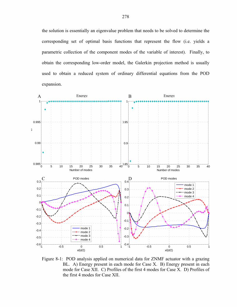
278

the solution is essentially an eigenvalue problem that needs to be solved to determine the

corresponding set of optimal basis functions that represent the flow (i.e. yields a

parametric collection of the component modes of the variable of interest). Finally, to

obtain the corresponding low-order model, the Galerkin projection method is usually

used to obtain a reduced system of ordinary differential equations from the POD

expansion.

Figure 8-1: POD analysis applied on numerical data for ZNMF actuator with a grazing

BL. A) Energy present in each mode for Case X. B) Energy present in each mode for Case XII. C) Profiles of the first 4 modes for Case X. D) Profiles of the first 4 modes for Case XII.

0 5 10 15 20 25 30 35 400.85

0.9

0.95

1

Number of modes

Ene

rgy

0 5 10 15 20 25 30 35 400.985

0.99

0.995

1

Number of modes

gy

A B Energy Energy

-1 -0.5 0 0.5 1-0.6

-0.5

-0.4

-0.3

-0.2

-0.1

0

0.1

0.2

0.3

x/(d/2)

POD modes

mode 1mode 2mode 3mode 4

-1 -0.5 0 0.5 1-0.4

-0.3

-0.2

-0.1

0

0.1

0.2

0.3

0.4

x/(d/2)

POD modes

mode 1mode 2mode 3mode 4

D C

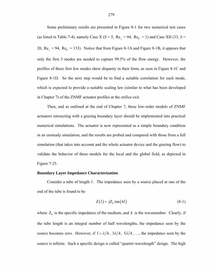
279

Some preliminary results are presented in Figure 8-1 for two numerical test cases

(as listed in Table 7-4), namely Case X (S = 5, Re j = 94, Reθ = 1) and Case XII (33, S =

20, Re j = 94, Reθ = 133). Notice that from Figure 8-1A and Figure 8-1B, it appears that

only the first 3 modes are needed to capture 99.5% of the flow energy. However, the

profiles of these first few modes show disparity in their form, as seen in Figure 8-1C and

Figure 8-1D. So the next step would be to find a suitable correlation for each mode,

which is expected to provide a suitable scaling law (similar to what has been developed

in Chapter 7) of the ZNMF actuator profiles at the orifice exit.

Then, and as outlined at the end of Chapter 7, these low-order models of ZNMF

actuators interacting with a grazing boundary layer should be implemented into practical

numerical simulations. The actuator is now represented as a simple boundary condition

in an unsteady simulation, and the results are probed and compared with those from a full

simulation (that takes into account and the whole actuator device and the grazing flow) to

validate the behavior of these models for the local and the global field, as depicted in

Figure 7-25.

Boundary Layer Impedance Characterization

Consider a tube of length l . The impedance seen by a source placed at one of the

end of the tube is found to be

( ) ( )0 tanZ l jZ kl= (8-1)

where 0Z is the specific impedance of the medium, and k is the wavenumber. Clearly, if

the tube length is an integral number of half wavelengths, the impedance seen by the

source becomes zero. However, if 4l λ= , 3 4λ , 5 4λ , …, the impedance seen by the

source is infinite. Such a specific design is called “quarter-wavelength” design. The high

280

impedance of a quarter-wavelength open tube is sometimes used for applications, such as

the study of sound propagation in a duct in which the air is moving, as shown in Figure

8-2.

Source

Air in Air out

Air flow

λ/4 λ/4

Figure 8-2: Use of quarter-wavelength open tube to provide an infinite impedance.

(Adapted from Blackstock 2000)

Here, consider the case in which the cavity depth of a ZNMF device is a quarter of

the wavelength of interest. The cavity impedance becomes infinite, thereby leaving only

the boundary layer impedance of the crossflow superimposed on the orifice impedance.

If the orifice dimensions are judiciously chosen such that the flow inside the orifice is

well behaved and has a validated model, it will then be possible to isolate the BL

impedance for analysis, thereby extracting a low-order model to be implemented as a

design tool.

MEMS Scale Implementation

Several previous works on ZNMF actuators have proposed the use of MEMS

devices (Mallison et al. 2003, 2004) as opposed to the meso-scale devices usually

employed, as in this dissertation. MEMS-based actuators consist of devices that have

been fabricated using silicon micromachining technology (see for example Madou

(1997)). A candidate MEMS ZNMF actuator can be designed using fundamental

structural models and lumped element models previously developed, such as

thermoelastic (Chandrasekaran et al. 2003) and piezoelectric (Wang et al. 2002)

actuators.

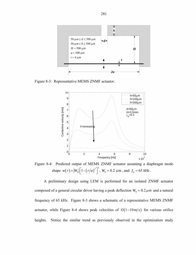
281

d

h

H

t

2a

50 500 50 500

500 500 4

m d mm h m

H ma mt m

µ ≤ ≤ µµ ≤ ≤ µ= µ= µ= µ

Figure 8-3: Representative MEMS ZNMF actuator.

0 2 4 6 8 10

x 104

0

1

2

3

4

5

6

7

8

9

10

Frequency [Hz]

Cen

terli

ne v

eloc

ity [m

/s]

h=50µmh=100µmh=500µm

d=50µmH=0.5mmζd=0.1

h increasing

Figure 8-4: Predicted output of MEMS ZNMF actuator assuming a diaphragm mode

shape ( ) ( )22

0 1w r W r a⎡ ⎤= −⎣ ⎦ , 0 0.2 W mµ= , and 65 df kHz= .

A preliminary design using LEM is performed for an isolated ZNMF actuator

composed of a general circular driver having a peak deflection 0 0.2W mµ= and a natural

frequency of 65 kHz. Figure 8-3 shows a schematic of a representative MEMS ZNMF

actuator, while Figure 8-4 shows peak velocities of ( )1 10O m s− for various orifice

heights. Notice the similar trend as previously observed in the optimization study

282

performed in Gallas et al. (2003b). These promising results suggest that a MEMS ZNMF

actuator is capable of producing a reasonable velocity jet.

An interesting analysis will be to investigate the effect of scaling the results found

in this dissertation for the meso-scale down to the MEMS scale, and to examine the

corresponding effects with the intrinsic limitations. Also, an appropriate review on the

relevance of such micro-devices in flow-control applications must be discussed.

Design Synthesis Problem

In Gallas et al. (2003b), the author performed an optimization of an isolated ZNMF

actuator, decoupling the driver optimization to the actuator cavity and orifice

optimization. However, it was limited to improving an existing baseline design. A more

interesting, though more challenging, case is the optimal design synthesis problem. In

this problem, the designer seeks to achieve a desired frequency response function. Due to

the nonlinear nature of the system, the design objective can be approximated by a linear

transfer function that is valid at a particular driving voltage. A key challenge here is that

the end user must be able to translate desirable actuator characteristics into quantitative

design goals.

283

Equation Chapter 1 Section 1 APPENDIX A

EXAMPLES OF GRAZING FLOW MODELS PAST HELMHOLTZ RESONATORS

It should be noted that this discussion is far from exhaustive. Even several versions

may exist for each model presented. The first model presented is from Rice (1971) and is

based on the continuity and momentum equations through the orifice while the cavity is

lumped as a simple spring model. The results yield the following model of the

normalized specific impedance of the orifice subjected to grazing flow

( )p pj jζ θ χ σ θ χ= + = + , (A-1)

where the normalized specific resistance pθ of an array of resonators is given by

0,

0 0grazing flowviscous losses

0.381pp

R Mhc d c

νωθρ σ σ

∞⎛ ⎞= = + +⎜ ⎟⎝ ⎠

, (A-2)

and the normalized specific reactance pχ for an array of resonators is

( )0,

30

0.85 1 0.7

1 305p

p

X k hc M

σχ

ρ σ ∞

⎡ ⎤−⎢ ⎥= = +⎢ ⎥+⎣ ⎦

. (A-3)

Here 0, pR and 0, pX represent, respectively, the specific resistance and reactance of

the perforate, 0cρ is the characteristic impedance of the medium, ν is the kinematic

viscosity, σ is the porosity of the perforate, d is the orifice diameter, h is the thickness

of the orifice, ω is the radian frequency, and k is the wavenumber, and M∞ is the

grazing flow Mach number. The model is validated with data using the two-pressure

284

measurement method obtained by Pratt & Whitney (see Garrison 1969) and the Boeing

Company. Rice (1971) made the following remark regarding the data provided: “The

data at 0U∞ = are questionable since the electro-pneumatic driver provided substantial

air flow which had to be bled off before reaching the sample and recirculating flows

resulted (conversation with Garrison).” Therefore, this model may not work well at

0M∞ = .

Next, Bauer (1977) proposed the following empirical normalized specific

impedance model containing the influence of crossflow velocity:

( ) ( )0

0 0

1.15 0.258 0.31 1 bu c k h dMp h jc u c d

χθ

µωζ

ρ σ σ σ σ∞

⎡ ⎤⎛ ⎞ +⎡ ⎤′ ⎛ ⎞= = + + + +⎢ ⎥⎜ ⎟ ⎢ ⎥⎜ ⎟⎜ ⎟′ ⎝ ⎠⎢ ⎥ ⎣ ⎦⎝ ⎠⎣ ⎦, (A-4)

where p′ and u′ are respectively the acoustic pressure and particle velocity, and bu is

the bias flow velocity through the perforate (steady flow). Notice that in this model, the

grazing flow affects only the resistance part of the impedance and not the reactance.

Figure A-1 shows the test apparatus used. The liners were tested using the two

microphone technique, a microphone being mounted at the bottom of the liner cavity and

another one on the liner surface. The incoming grazing flow has become fully turbulent

by the time it has reached the test panel and a boundary layer survey showed a velocity

profile close to the 1/7 power shape.

285

absorptive liners

test panel

acoustic wave fronts

microphone

sirenhorn

air inlet

ductflow

Figure A-1: Acoustic test duct and siren showing a liner panel test configuration. (Adapted from Bauer 1977).

Another model is presented by Hersh and Walker (1979). They derive a semi-

empirical impedance model for a single orifice, where it is assumed that the sound

particle enters the resonator cavity in a spherical, radically manner during the inflow half-

cycle, following a vena contracta path. For non-zero grazing flow, they predict the

following orifice area-averaged normalized resistance and reactance

( )

0

0 1.87 0.17R Mc dρ δ

∞=+

, (A-5)

and

( ) ( )

( )

1 3

0 0

0

0.14 2.07 0.43ln 3.7 2.63

1.19 0.11

d E EX cc d

ω ε α ε

ρ δ

⎡ ⎤− − −⎢ ⎥⎣ ⎦=

+, (A-6)

where the quantity ( ) 8D iE C d Pε ρ ω 2= , with iP being the incident pressure, and

( ) ( )2 8H D eC d dα ω ω= , with the orifice inertial length being defined by

( )0.85 1 1.25e cd h d d D= + − . Here ( ) 0 0 cR A A p u′ ′= ℜ and ( ) 0 0 cX A A p u′ ′= ℑ

are respectively the area-averaged (ratio of orifice to cavity cross sectional area) specific

resistance and reactance of the orifice. Notice that in this model representation, the

286

grazing flow effects is only seen in the resistance part of the impedance, and that no

viscous losses in the orifice are represented. A schematic of the apparatus setup and

instrumentation hardware used is given in Figure A-2. Extensive experimental data have

been reported, from single to clustered orifices, thin perforate plate to thick orifices and

within a large range of SPL and grazing flow velocity. For the purpose of this

dissertation, only the thick orifices database is taken, as documented in Table A-1 at the

end of this Appendix.

0.125 m Mic.

0.125 m Mic.

0.10 m 0.125 m

d

0.25 m

τ

L

DPc

Pi

Orifice

HorncouplerDriver

poweramplifier oscillator digital

phase

Synch.FilterMtr.

DVM 1/10 Oct.analyser

Figure A-2: Schematic of test apparatus used in Hersh and Walker (1979). (Adapted from Hersh and Walker 1979)

287

Following the previous work done by Cummings (1986), Kirby and Cummings

(1998) measured the acoustic impedance of perforates with and without a porous

backing. An empirical model of perforates without porous backing is given by

0.169

0 26.16 20 4.055f c uhfd d fd

θ −∗

⎧ ⎫⎪ ⎪⎛ ⎞= − −⎨ ⎬⎜ ⎟⎝ ⎠⎪ ⎪⎩ ⎭

, (A-7)

for the normalized flow induced resistance of the orifice, and the mass end correction by

0

0

1 0.18

1 0.6 exp 0.18 1.8 0.6 0.18

uh dh fh h

uh h h du d hfh h dh d d fh h

∗

∗∗

⎧ ′ ⎛ ⎞= ≤⎪ ⎜ ⎟

⎝ ⎠⎪⎨

⎧ ⎫′ ⎛ ⎞⎛ ⎞⎛ ⎞ ⎛ ⎞⎪ = + − − + − >⎨ ⎬⎜ ⎟ ⎜ ⎟⎜ ⎟ ⎜ ⎟⎪ ⎝ ⎠⎝ ⎠ ⎝ ⎠ ⎝ ⎠⎩ ⎭⎩

.(A-8)

The acoustic impedance is normalized such that

00

0f

Z ic

ζ θ θ χρ

= = + + , (A-9)

where ( )( )0 0, p cZ A A p u′ ′= is the specific area-averaged impedance of the perforate,

0, pA being here the total area of all orifices in the perforate test sample and cA the cavity

cross-sectional area. Here the orifice resistance due to viscous loss is given by

00

8 ,hc dνωθ = (A-10)

and the normalized orifice reactance can be obtained from the end correction ratio 0h h′

given by Eq. A-8 and by the following relation,

( )0

0.85hk h dh

χ⎡ ⎤′

= +⎢ ⎥⎣ ⎦

, (A-11)

288

Power amplifier

Thandar TG503signal

generator

Ono SokkiCF-35OZ FFT

analyser

test cavityJBL 2445Jcompressor driver

air in

duct

2.5 m 0.4 m

33 mm33 mm

72 mm 72 mm

duct

cavity

perforate

Bruel & Kjoer1/2" condensermicrophonesType 4134

sectionthrough duct

and test cavity

Figure A-3: Apparatus for the measurement of the acoustic impedance of a perforate used by Kirby and Cummings (1998). (Adapted from Kirby and Cummings 1998)

289

under the assumption that the end correction length without flow is approximately equal

to 0.85d for an isolated orifice if d λ , λ being the wavelength. This last assumption

is discussed in more rigorous details by Ingard (1953) and is used to eliminate the jetting

interaction effect due to closely spaced orifices in a flat plate. In this model the friction

velocity is a function of the rectangular duct area based Reynolds number, as discussed

by Cummings (1986). Notice that this model is a function of the inverse of Strouhal

number based on the grazing flow friction velocity and on either the diameter or the

thickness of the orifice, and shows two different regimes for the reactance model function

of the orifice aspect ratio. The experiments were performed for different Helmholtz

resonator configurations as listed in Table A-1, the grazing flow being fully turbulent by

the time it reaches the test section. The experimental setup is shown in Figure A-3.

Finally, the last model presented in this dissertation is the so-called NASA Langley

Zwikker-Kosten Transmission Line Code (ZKTL), and is presented in Betts (2000). It is

based on transmission matrix theory, and the contribution from the grazing flow can be

taken from the boundary condition of the problem. The full normalized orifice

impedance of the perforate sheet (including bias flow into the orifice) is given below by

( ) ( )

02

0 00

12 2 1.256

f bp a

D

R c uv Mc cc C d

θδρ σ σ

∞

⎡ ⎤= + + +⎢ ⎥

+⎣ ⎦ (A-12)

for the resistance part, and by

30

0.85 1 0.721 305D

dfX hc C M

σπσ ∞

⎡ ⎤⎡ ⎤−⎣ ⎦⎢ ⎥= +⎢ ⎥+⎣ ⎦

(A-13)

for the reactance part. Here, av is a dimensionless acoustic particle velocity, bu is the

bias flow velocity through the orifice, and fR corresponds to a linear input flow

290

resistance of the perforated sheet. This model finds its origins in the work done by Hersh

and Walker (1979) (presented above) and Heidelberg et al. (1980) for the resistance part,

and by Rice (1971) (see above) and Motsinger and Kraft (1991) for the reactance part of

the impedance. The database used in this model is directly taken from previous works,

most of which being already listed herein. Figure A-4 depicts a typical acoustic liner and

the NASA impedance tube.

1. High pressure air2. Traversing mic.3. Acoustic drivers4. Plenum

5. Reference mic.6. Test section with liner7. Termination8. To vacuum pumps

1

2

5 6 7 843

Figure A-4: Sketch of NASA Grazing Impedance Tube. (Adapted from Jones et al.

2003).

Table A-1: Experimental database for grazing flow impedance models References M∞ σ (%) d (mm) Rice (1971) 0 0.26 0.01 0.21 1.19 2.51 Bauer (1977) 0.2 0.6 0.21 1.2 Hersh & Walker (1979) 0 0.23 single orifice 1.78 Kirby & Cummings (1986)

0.47 2.19 (based on u∗ )

0.20 0.27

2.8 3.5

t (mm) f (Hz) iP (dB) Rice (1971) 1.29 6.35 1600 2600 130 168 Bauer (1977) 0.64 800 1400 116 136 Hersh & Walker (1979) 0.5 8.9 197 552 70 140 Kirby & Cummings (1986) 1.0 1.5 70 1000 N/A

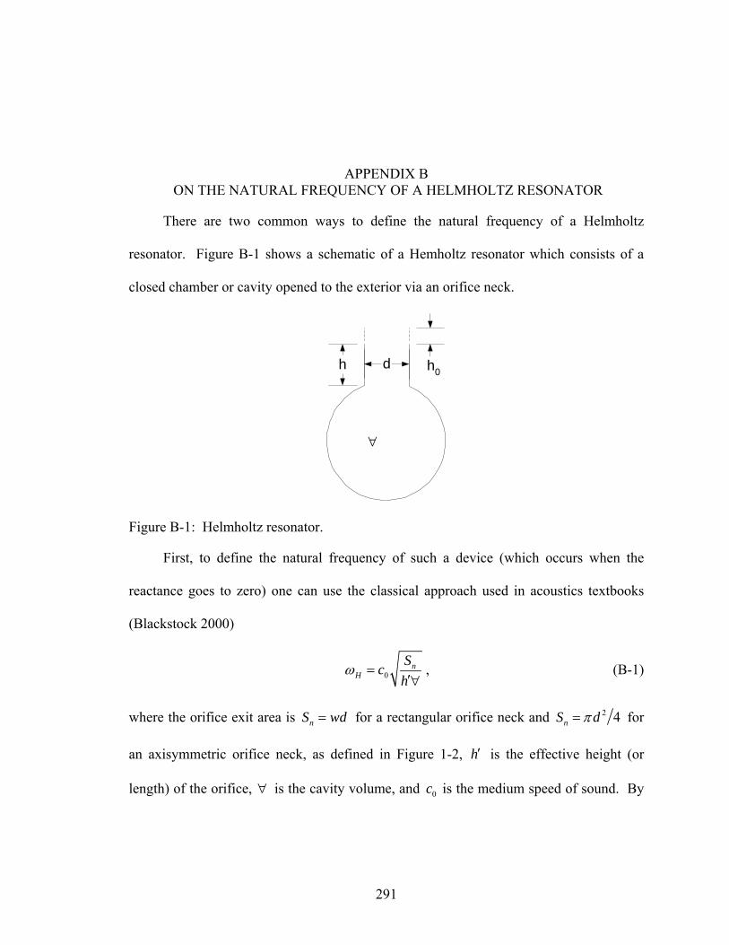
291

Equation Chapter 2 Section 1 APPENDIX B

ON THE NATURAL FREQUENCY OF A HELMHOLTZ RESONATOR

There are two common ways to define the natural frequency of a Helmholtz

resonator. Figure B-1 shows a schematic of a Hemholtz resonator which consists of a

closed chamber or cavity opened to the exterior via an orifice neck.

h d

∀

h0

Figure B-1: Helmholtz resonator.

First, to define the natural frequency of such a device (which occurs when the

reactance goes to zero) one can use the classical approach used in acoustics textbooks

(Blackstock 2000)

0n

HSch

ω =′∀

, (B-1)

where the orifice exit area is nS wd= for a rectangular orifice neck and 2 4nS dπ= for

an axisymmetric orifice neck, as defined in Figure 1-2, h′ is the effective height (or

length) of the orifice, ∀ is the cavity volume, and 0c is the medium speed of sound. By

292

definition, the effective length of the orifice is 0h h h′ = + , where 0h corresponds to the

“end correction.” Ingard (1953) provides a general definition,

Usually the end correction is indiscriminately taken as the mass end correction for a plane circular piston in an infinite plane, which equals ( ) 0 016 3 1.7r rπ , where 0r is the radius of the piston or the circular aperture. To make it applicable for an arbitrary aperture, the end correction is sometimes written 0 0.96 nh S= … A careful analysis should actually consider different end corrections on the two sides of the aperture so that 0 0, 0,e ih h h= + , the sum of an exterior end correction 0,eh and an interior correction 0,ih .

Thus, in the case of a circular orifice, the value for the exterior end correction can

be taken as 0, 0.85 0.96e nh d S . The interior correction can be approximated for low

values of ξ ( 0.4ξ < , the ratio of the orifice diameter to the cavity diameter) by

( )0, 0.48 1 0.25i nh S ξ− , and tends to zero for ξ close to one, as found in Ingard (1953)

for concentric circular and square apertures in a tube.

On the other hand, one can define the Helmholtz frequency of a resonator by

directly using lumped elements: the fluid inside the closed cavity in Figure B-1 acts like a

spring and that in the orifice neck like a mass, the system thus behaves like a simple

oscillator. The natural frequency of the resonator being that at which the reactive part of

the impedance vanishes,

1H

aC aNC Mω = , (B-2)

where 20aCC cρ= ∀ is the acoustic compliance of the cavity and aNM is the acoustic

mass of the neck. As derived in Appendix C, aNM is given by

( )2axisym.

4

3 2aN

hMdρ

π= , and

( )rect.

35 2

aNhM

dwρ

= . (B-3)

293

Thus, the Helmholtz frequency for an axisymmetric and for a rectangular orifice is,

respectively

( )

220

0axisym.

32 0.86

4n

H

d cSc

h h

πω

⎛ ⎞⎜ ⎟⎝ ⎠= =

∀ ∀, (B-4)

and

( )20

0rect.

52 0.91

3n

H

dw cSc

h hω

⎛ ⎞⎜ ⎟⎝ ⎠= =∀ ∀

. (B-5)

It is interesting to compare Eqs. B-4 and B-5 with Eq. B-1, which only differ by the

end correction effect. For example, consider a Helmholtz resonator in still air at STP

conditions having a cavity volume 31000mm∀ = and first a circular orifice of

dimensions ( ) ( ), 2,5d h mm= , and then a rectangular orifice of dimensions

( ) ( ), , 2,5,10d h w mm= . Substituting in the above equations yield the results listed in

Table B-1. Clearly, the two definitions give similar results and can be used

interchangeably.

Table B-1: Calculation of Helmholtz resonator frequency. Eq. B-1 Eq. B-4 Eq. B-5

axisym. 1189 1184

2H

Hfωπ

= [Hz] rect. 3000 3160

Therefore, for a general purpose discussion, to within a constant multiplier, the

Helmholtz frequency scales as

0 0n n

HS Sc ch h

ω = ∝′∀ ∀

, (B-6)

294

where nS wd= for a rectangular slot and 2 4nS dπ= for an axisymmetric orifice, and

0h h h′ = + with the end correction 0 0.96 nh S= . Eq. B-6 is used throughout this

dissertation for scaling analysis unless specifically stated, while Eqs. B-1, B-4 or B-5 are

employed as needed to estimate dimensional values.

295

APPENDIX C

DERIVATION OF THE ORIFICE IMPEDANCE OF AN OSCILLATING PRESSURE DRIVEN CHANNEL FLOW

h

wx

y

z

d

Figure C-1: Rectangular slot geometry and coordinate axis definition

Assuming a fully-developed, laminar, unsteady, and incompressible flow through a

two-dimensional channel, the continuity equation confirms that the only non-zero

velocity is ( )v v x= .

The y −momentum equation gives

v ut

ρ ρ∂+

∂v vvx y

ρ∂ ∂+

∂ ∂

2 2

2 2

p v vy x y

µ∂ ∂ ∂= − + +

∂ ∂ ∂

⎛ ⎞⎜ ⎟⎜ ⎟⎝ ⎠

, (C-1)

which reduces to

2

2

v p vt y x

ρ µ∂ ∂ ∂= − +

∂ ∂ ∂, (C-2)

having boundary conditions:

4. ( )0v x = < ∞ (finite velocity at the centerline)

5. ( )2 0v x d= ± = (no-slip condition) The solution of Eq. C-2 takes the form

296

complimentary

particular( , ) ( )

i t

i t

v

p P ey h

v x t A x e v

ω

ω

∂ ∆⎧ = −⎪∂⎪⎨

= +⎪⎪⎩

(C-3)

First, substituting complimentaryv in Eq. C-2 gives

2

2

A i PAx h

ωρµ µ

∂ ∆− = −

∂, (C-4)

and by letting α ωρ µ= and P hβ µ= −∆ , Eq. C-4 then becomes

A i Aα β′′ − = , (C-5)

which has for its solution ( ) ( ) ( )1 2cosh sinhA x C x C xγ γ= + . Applying the

boundary condition (i) yields 2 0C = and 2i dγ = , where 1i = − is the complex

number and 1C is a constant of integration to be determined later. Therefore, the

complimentary solution of Eq. C-3 is

( )complimentary , ( ) coshi t i tv x t A x e C i x eω ωρων

⎛ ⎞= = ⎜ ⎟⎜ ⎟

⎝ ⎠. (C-6)

Similarly, the particular solution of Eq. C-3 can easily be found to be

( )particular , i tPv x t i eh

ω

ωρ∆

= − . (C-7)

Next, substituting Eqs. C-6 and C-7 in Eq. C-3, applying the boundary condition

(ii) and solving for the constant 1C gives

1

cosh2

PC idh i ρωρω

µ

∆=

⎛ ⎞⎜ ⎟⎝ ⎠

. (C-8)

Therefore, the solution of Eq. C-2 for a rectangular channel is finally given by

297

cosh

( , ) 1cosh

2

i t

x iPv x t i eh d i

ω

ρωµ

ρω ρωµ

⎧ ⎫⎛ ⎞⎪ ⎪⎜ ⎟

∆ ⎪ ⎪⎝ ⎠= − −⎨ ⎬⎛ ⎞⎪ ⎪⎜ ⎟⎪ ⎪⎝ ⎠⎩ ⎭

. (C-9)

A special case of interest arises for low operational frequencies. For 1ω , then

1iω ν , and since the Taylor series expansion of the hyperbolic cosine is given by

2 4

cosh( ) 1 ...2 24x xx = + + + , (C-10)

therefore, for small ω , Eq. C-9 can be rewritten as

2

2

12( , ) 1

12 2

i ti xPv x t i e

h di

ω

ων

ρω ων

⎧ ⎫⎪ ⎪+∆ ⎪ ⎪= − −⎨ ⎬

⎛ ⎞⎪ ⎪+ ⎜ ⎟⎪ ⎪⎝ ⎠⎩ ⎭

, (C-11)

or,

( ) ( ) ( ) ( ) 2 2

2

2, cos sin

21

2 2

d xPv x t t i th di

ω ωρν ω

ν

⎡ ⎤⎢ ⎥−∆ ⎢ ⎥= +⎢ ⎥⎛ ⎞+⎢ ⎥⎜ ⎟

⎝ ⎠⎣ ⎦

. (C-12)

Taking the real part,

( ) ( )

( )( ) ( ) ( ) ( )2 2 2

42 2

2 2 2Re , cos sin

24 2

P d x dv x t t t

h d

ν ωω ω

νρ ν ω

⎡ ⎤∆ − ⎧ ⎫⎪ ⎪⎣ ⎦= +⎨ ⎬+ ⎪ ⎪⎩ ⎭

, (C-13)

and since for small ω , 2 1ω , cos( ) 1tω ≈ and sin( ) 0tω ≈ , hence

2

2( )2 2

P dv x xhµ⎡ ⎤∆ ⎛ ⎞= −⎢ ⎥⎜ ⎟⎝ ⎠⎢ ⎥⎣ ⎦

, (C-14)

which is, as expected, the solution for the steady channel flow.

298

Now, assuming low operational frequencies ( )0 1kd d cω= , one can extract the

corresponding lumped parameters as follow:

Since jQ represents the volume flow rate of the orifice, thus

22

2 2

0 2 2( ) 1

2 2 2w d d

j d d

I

w P d xQ v x dxdz dxh dµ− −

⎡ ⎤⎛ ⎞∆ ⎛ ⎞= = −⎢ ⎥⎜ ⎟⎜ ⎟⎝ ⎠ ⎢ ⎥⎝ ⎠⎣ ⎦

∫ ∫ ∫ , (C-15)

and the integral I is found to be

( )

23

2

2

43 23 2

d

d

x dI xd

−

⎡ ⎤ ⎛ ⎞= − =⎢ ⎥ ⎜ ⎟⎝ ⎠⎢ ⎥⎣ ⎦

. (C-16)

Therefore,

( )32 23j

w P dQ

hµ∆

= . (C-17)

The dissipative term aNR , that represents the acoustic resistance due to viscous

losses in the orifice, is represented in LEM with effort-flow variables by

aNj

e PRf Q

∆= = . (C-18)

Hence, one can obtain the expression of the viscous resistance in the 2D slot:

( )33

2 2aN

hRw dµ

= . (C-19)

The kinetic energy of the fully-developed flow in the channel can be expressed by

222

2 20

2

1 1 12 2 2

d

KE aN jd

I

xW M Q h v wdxd

ρ−

′

⎧ ⎫⎛ ⎞⎪ ⎪= = −⎨ ⎬⎜ ⎟⎝ ⎠⎪ ⎪⎩ ⎭

∫ , (C-20)

where

299

22

0 02

412 3 2

d

jd

x w dQ v wdx vd−

⎛ ⎞⎛ ⎞ ⎛ ⎞⎜ ⎟= − =⎜ ⎟ ⎜ ⎟⎜ ⎟ ⎝ ⎠⎝ ⎠⎝ ⎠∫ , (C-21)

and 0v being the centerline velocity given by

2

0 2 2P dvhµ

∆ ⎛ ⎞= ⎜ ⎟⎝ ⎠

. (C-22)

Then, since the integral I ′ is equal to

( ) ( )

23 5

2 4

2

2 1 163 5 15 22 2

d

d

x x dI xd d

−

⎡ ⎤ ⎛ ⎞′ = − + =⎢ ⎥ ⎜ ⎟⎝ ⎠⎢ ⎥⎣ ⎦

, (C-23)

the kinetic energy can be rewritten such as

( )

( )( )

( )

2 202

2

202

0

2

16 21 12 2 15

16 21 32 4 2 15

1 3 .2 5 2

jKE aN j

j

j

j

Q v dW M Q w w

Q

v dwQ h w

wv d

Q hw d

ρ

ρ

ρ

⎛ ⎞⎛ ⎞= = ⎜ ⎟⎜ ⎟⎜ ⎟⎝ ⎠⎝ ⎠

⎛ ⎞⎛ ⎞= ⎜ ⎟⎜ ⎟⎜ ⎟⎝ ⎠⎝ ⎠

=

(C-24)

Therefore, the expression of the acoustic mass of the rectangular orifice is given by

( )

35 2aN

hMw dρ

= . (C-25)

Oscillatory pressure-driven pipe flow:

In a similar manner, the solution of oscillating pressure driven pipe flow is derived

for a circular orifice geometry and can be found to be

300

0

0

( , ) 1

2

i t

iJ rPv r t i eh d iJ

ω

ων

ωρ ων

⎧ ⎫⎛ ⎞−⎪ ⎪⎜ ⎟

∆ ⎪ ⎪⎝ ⎠= − −⎨ ⎬⎛ ⎞⎪ ⎪−⎜ ⎟⎪ ⎪⎝ ⎠⎩ ⎭

, (C-26)

where 0J is a Bessel function of zero order. Again via a low frequency assumption, the

velocity profile becomes that of a Poiseuille flow:

2

2( )4 2

P dv r rhρν⎡ ⎤∆ ⎛ ⎞= −⎢ ⎥⎜ ⎟⎝ ⎠⎢ ⎥⎣ ⎦

. (C-27)

From there, the lumped element parameters are extracted, and the acoustic

resistance and mass of the orifice impedance are given by, respectively

( )48

2aN

hRdµ

π= , and

( )24

3 2aN

hMdρ

π= . (C-28)

Another special case of interest occurs for very high frequencies. In this case, the

zero-order Bessel function can be approximate by

( )02 cos

4J z z

zπ

π⎛ ⎞= −⎜ ⎟⎝ ⎠

. (C-29)

So the velocity can be rewritten as

( )

2 cos4

, 12 2 cos

2 4

cos421

cos2 4

i t

i t

irr iPv r t i e

h d id i

irdPi e

h r d i

ω

ω

ω πνπ ω ν

ωρ ω πνπ ω ν

ω πν

ωρ ω πν

⎧ ⎫⎛ ⎞−−⎪ ⎪⎜ ⎟

−∆ ⎪ ⎪⎝ ⎠= − −⎨ ⎬⎛ ⎞⋅ −⎪ ⎪−⎜ ⎟⎪ ⎪− ⎝ ⎠⎩ ⎭

⎧ ⎫⎛ ⎞−−⎪ ⎪⎜ ⎟

∆ ⎪ ⎪⎝ ⎠= − −⎨ ⎬⎛ ⎞−⎪ ⎪−⎜ ⎟⎪ ⎪⎝ ⎠⎩ ⎭

(C-30)

Using some trigonometric identity,

301

4 4 4 4

2 4 2 4 2 24 4

cos4

cos2 4

i i i ir r r r

d i d i d i d i

ire e e e e e

d ie e e e e e

ω π ω π ω ωπ πν ν ν ν

ω π ω π ω ωπ πν ν ν ν

ω πν

ω πν

− − − −− − + −−

− − − −− − + −−

⎛ ⎞−−⎜ ⎟

+ ⋅ + ⋅⎝ ⎠ = =⎛ ⎞−

− + ⋅ + ⋅⎜ ⎟⎝ ⎠

, (C-31)

and since ( )4 1 2e iπ− = + , and ( )4 1 2ii e iπ−− = = − , Eq. C-31 becomes

( )( )

( )( )1 1

2 2cos

4 1 1

cos2 4

i r i rir

i e i e

d i

ω ων ν

ω πν

ω πν

+ − +⎛ ⎞−

−⎜ ⎟− + +⎝ ⎠ =

⎛ ⎞−−⎜ ⎟

⎝ ⎠( )

( )( )

( )1 12 2 2 21 1d di i

i e i eω ων ν

+ − +− + +

( ) ( )1 22

i r de

ων

+ −= , (C-32)

where the two terms vanished at high frequency ( )1ω . Substituting Eq. C-32 in Eq.

C-30 yields

( )( ) ( )1 2

22, 1i r di t dPv r t i e e

h r

ωω ν

ωρ+ −⎧ ⎫∆ ⎪ ⎪= − −⎨ ⎬

⎪ ⎪⎩ ⎭, (C-33)

or by expending the exponential terms,

( ) ( ) ( )

2 2

, cos sin

21 cos sin2 2 2 2

dr

Pv r t i i t th

d d de r i rr

ων

ω ωωρ

ω ων ν

⎛ ⎞−⎜ ⎟⎝ ⎠

∆= − − +⎡ ⎤⎣ ⎦

⎧ ⎫⎡ ⎤⎛ ⎞ ⎛ ⎞⎪ ⎪⎛ ⎞ ⎛ ⎞⋅ − − + −⎢ ⎥⎜ ⎟ ⎜ ⎟⎨ ⎬⎜ ⎟ ⎜ ⎟⎜ ⎟ ⎜ ⎟⎝ ⎠ ⎝ ⎠⎢ ⎥⎝ ⎠ ⎝ ⎠⎪ ⎪⎣ ⎦⎩ ⎭

(C-34)

Taking the real part of Eq. C-34 gives then the final expression of the velocity in

the large frequency range,

( ) ( ) 2 22, sin sin2 2

drd dPv r t i t e t rh r

ων ωω ω

ωρ ν

⎛ ⎞−⎜ ⎟⎝ ⎠

⎧ ⎫⎛ ⎞∆ ⎪ ⎪⎛ ⎞= − − ⋅ − −⎜ ⎟⎨ ⎬⎜ ⎟⎜ ⎟⎝ ⎠⎝ ⎠⎪ ⎪⎩ ⎭. (C-35)

Viscothermal analysis:

The nondimensional energy equation for a circular pipe, assuming an ideal gas

( )p RTρ= , small perturbations and time harmonic wave field, can be reduced to

302

( )2

22 2 2

1 1Pr

T T pkdt S y t

γγ

∗ ∗ ∗

∗ ∗ ∗

∂ ∂ − ∂= +

∂ ∂ ∂, (C-36)

where Pr ν α= is the Prandtl number (the ratio of the viscous to thermal diffusivity), S

is the Stokes number and γ is the ratio of specific heats. Furthermore, neglecting higher-

order terms, the equation of state for an ideal gas reduces to

p Tρ∗ ∗ ∗= + . (C-37)

After manipulations and simplifications, if one assumes the tube is small in

comparison with the wave length (kd << 1), the temperature profile is given by

( )1 Pr

21 1j S y

T y p eγγ

∗+−

∗∞

⎛ ⎞−= −⎜ ⎟⎜ ⎟

⎝ ⎠. (C-38)

The thermal boundary layer is then

6.5Pr Prthν δδ

ω≈ = . (C-39)

Since in air the Prandtl number is about 0.7, the viscous boundary layer δ and the

thermal boundary layer thδ are of the same order of magnitude and have the same

frequency dependence.

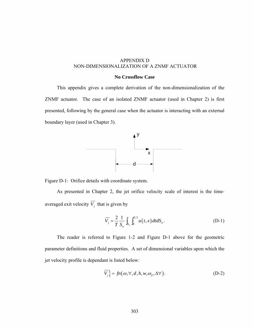
303

Equation Chapter 4 Section 1 APPENDIX D

NON-DIMENSIONALIZATION OF A ZNMF ACTUATOR

No Crossflow Case

This appendix gives a complete derivation of the non-dimensionalization of the

ZNMF actuator. The case of an isolated ZNMF actuator (used in Chapter 2) is first

presented, following by the general case when the actuator is interacting with an external

boundary layer (used in Chapter 3).

d

x

y

Figure D-1: Orifice details with coordinate system.

As presented in Chapter 2, the jet orifice velocity scale of interest is the time-

averaged exit velocity jV that is given by

( )2

0

2 1 ,n

T

j nSn

V u t x dtdST S

= ∫ ∫ . (D-1)

The reader is referred to Figure 1-2 and Figure D-1 above for the geometric

parameter definitions and fluid properties. A set of dimensional variables upon which the

jet velocity profile is dependant is listed below:

( ), , , , , ,j dV fn d h wω ω= ∀ ∆∀ . (D-2)

304

The Buckingham-Pi theorem (Buckingham 1914) is then used to construct the Π -

groups in terms of the independent dimensional units M, L and T, respectively for Mass,

Length and Time. Table D-2 lists the dimensions of all variables. The number of

parameters is 11n = , and the rank of the matrix is 3. Thus 11 3 8− = Π -groups are

expected. The 3 primary variables chosen are the length scale d , the time scale ω , and

the density ρ (for mass scale).

Table D-1: Dimensional matrix of parameter variables for the isolated actuator case. [M] [L] [T]

jV 0 1 -1

ω 0 0 -1

∀ 0 3 0

d 0 1 0

h 0 1 0

w 0 1 0

dω 0 0 -1

∆∀ 0 3 0

0c 0 1 -1 ρ 1 -3 0 µ 1 -1 -1

The 14 Π -groups are computed as follow:

• 1ja b c

j

VV d

dω ρ

ωΠ = = .

• 2 3a b cd

dω ρ ∀

Π =∀ = .

• 3a b c hhd

dω ρΠ = = .

• 4a b c wwd

dω ρΠ = = .

• 5a b c d

Dd ωω ω ρω

Π = = .

305

• 6 3a b cd

dω ρ ∆∀

Π = ∆∀ = .

• 07 0

a b c cc dd

ω ρω

Π = = .

• 8 2 2a b cd

d dµ νµ ω ρ

ρω ωΠ = = = .

However, these Π -groups are not the only possible choice and, as long as all

primary Π -groups are used and appear in the linear product rearrangements, different

combinations can be made as shown below. For example, a new Π -group, i′Π , must

contain iΠ .

• 11

1

j

d StVω′Π = = =

Π is the Strouhal number.

• 2

2 32 2 3 2

4 7 0 0 H

h d d hd d w c wdc

ω ωωω

⎛ ⎞Π Π ∀ ∀′Π = = = =⎜ ⎟Π Π ⎝ ⎠ is the ratio of the driving

frequency to the Helmholtz frequency scales as 0H c wd h= ∀ω (see Appendix B for a complete discussion on Hω ), the measure of the compressibility of the flow in the cavity.

• 3 3hd

′Π = Π = is the orifice aspect ratio.

• 4 4wd

′Π = Π = is the orifice exit cross section aspect ratio.

• 55

1

d

′Π = =Π

ωω

is the ratio of the operating frequency to the natural frequency of

the driver.

• 3

66 3

2

dd

Π ∆∀ ∆∀′Π = = =Π ∀ ∀

is the ratio of the displaced volume by the driver to the

cavity volume.

• 77 0

1 d d kdcω

λ′Π = = = =

Π is the ratio of the orifice diameter to the acoustic

wavelength.

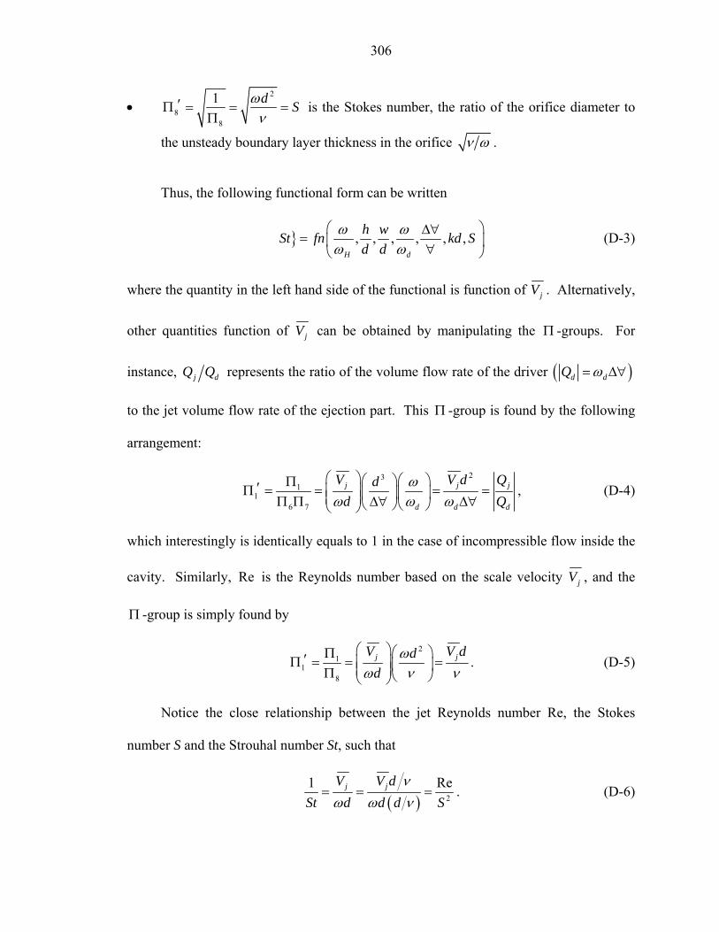
306

• 2

88

1 d Sων

′Π = = =Π

is the Stokes number, the ratio of the orifice diameter to

the unsteady boundary layer thickness in the orifice ν ω .

Thus, the following functional form can be written

, , , , , ,H d

h wSt fn kd Sd d

ω ωω ω⎛ ⎞∆∀

= ⎜ ⎟∀⎝ ⎠ (D-3)

where the quantity in the left hand side of the functional is function of jV . Alternatively,

other quantities function of jV can be obtained by manipulating the Π -groups. For

instance, j dQ Q represents the ratio of the volume flow rate of the driver ( )d dQ ω= ∆∀

to the jet volume flow rate of the ejection part. This Π -group is found by the following

arrangement:

23

11

6 7

j j j

d d d

V V d Qdd Q

ωω ω ω

⎛ ⎞ ⎛ ⎞⎛ ⎞Π′Π = = = =⎜ ⎟ ⎜ ⎟⎜ ⎟⎜ ⎟Π Π ∆∀ ∆∀⎝ ⎠⎝ ⎠⎝ ⎠, (D-4)

which interestingly is identically equals to 1 in the case of incompressible flow inside the

cavity. Similarly, Re is the Reynolds number based on the scale velocity jV , and the

Π -group is simply found by

2

11

8

j jV V ddd

ωω ν ν

⎛ ⎞⎛ ⎞Π′Π = = =⎜ ⎟⎜ ⎟⎜ ⎟Π ⎝ ⎠⎝ ⎠. (D-5)

Notice the close relationship between the jet Reynolds number Re, the Stokes

number S and the Strouhal number St, such that

( ) 2

1 Rej jV V dSt d d d S

νω ω ν

= = = . (D-6)

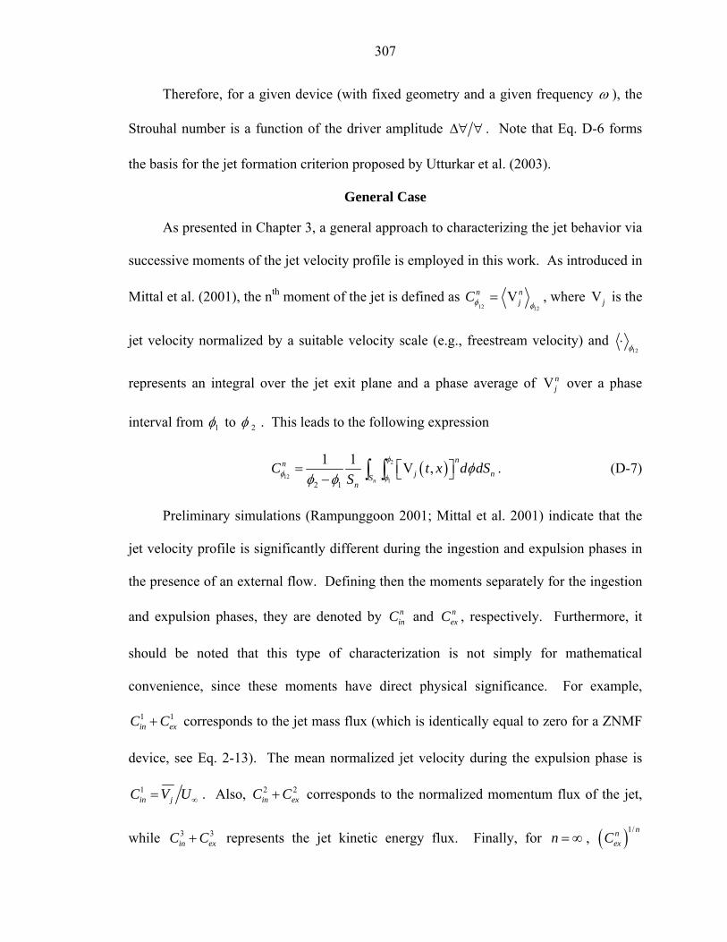
307

Therefore, for a given device (with fixed geometry and a given frequency ω ), the

Strouhal number is a function of the driver amplitude ∆∀ ∀ . Note that Eq. D-6 forms

the basis for the jet formation criterion proposed by Utturkar et al. (2003).

General Case

As presented in Chapter 3, a general approach to characterizing the jet behavior via

successive moments of the jet velocity profile is employed in this work. As introduced in

Mittal et al. (2001), the nth moment of the jet is defined as 12 12

n njCφ φ

= V , where jV is the

jet velocity normalized by a suitable velocity scale (e.g., freestream velocity) and 12φ

⋅

represents an integral over the jet exit plane and a phase average of njV over a phase

interval from 1φ to 2φ . This leads to the following expression

( )2

1212 1

1 1 ,n

nnj nS

n

C t x d dSS

φ

φ φφ

φ φ⎡ ⎤= ⎣ ⎦− ∫ ∫ V . (D-7)

Preliminary simulations (Rampunggoon 2001; Mittal et al. 2001) indicate that the

jet velocity profile is significantly different during the ingestion and expulsion phases in

the presence of an external flow. Defining then the moments separately for the ingestion

and expulsion phases, they are denoted by ninC and n

exC , respectively. Furthermore, it

should be noted that this type of characterization is not simply for mathematical

convenience, since these moments have direct physical significance. For example,

1 1in exC C+ corresponds to the jet mass flux (which is identically equal to zero for a ZNMF

device, see Eq. 2-13). The mean normalized jet velocity during the expulsion phase is

1in jC V U∞= . Also, 2 2

in exC C+ corresponds to the normalized momentum flux of the jet,

while 3 3in exC C+ represents the jet kinetic energy flux. Finally, for n = ∞ , ( )1/ nn

exC

308

corresponds to the normalized maximum jet exit velocity. Similarly, the skewness or

asymmetry of the velocity profile about the orifice center can be estimated as

( ) ( )2

1212 1

1 1 , ,n

j j nSn

X x x d dSS

φ

φ φφ φ φ

φ φ⎡ ⎤= − −⎣ ⎦− ∫ ∫ V V . (D-8)

A set of dimensional variables upon which the jet velocity profile is dependant is

listed below:

12

12

*0

7 device parameters 9 flow parameters

, , , , , , , , , , , , , , ,n

d w

Cfn d h w U c dP dx R

Xφ

φ

ω ω θ δ ρ µ τ∞ ∞ ∞

⎛ ⎞⎫⎪ ⎜ ⎟= ∀ ∆∀⎬⎜ ⎟⎪⎭ ⎝ ⎠

(D-9)

where the quantities in the left hand side of the functional form are the successive

moments and skewness of the jet velocity profile. The right hand side quantities are

either parameters of the actuator device or of the boundary layer.

Table D-2: Dimensional matrix of parameter variables for the general case. [M] [L] [T]

jV 0 1 -1 ω 0 0 -1 ∀ 0 3 0 d 0 1 0 h 0 1 0 w 0 1 0

dω 0 0 -1 ∆∀ 0 3 0 U∞ 0 1 -1 θ 0 1 0

*δ 0 1 0

0c 0 1 -1

∞ρ 1 -3 0

∞µ 1 -1 -1 dP dx 1 -2 -2

wτ 1 -1 -2

R 0 1 0

309

The Buckingham-Pi theorem (Buckingham 1914) is then used to construct the Π -

groups in terms of the independent dimensional units M, L and T, respectively for Mass,

Length and Time. Table D-2 lists the dimensions of all variables. The number of

parameters is 17n = (16 independent and 1 dependant), and the rank of the matrix is 3.

Thus 17 3 14− = Π -groups are expected. The 3 primary variables chosen are the length

scale d , the time scale ω , and the density ∞ρ (for mass scale).

The 14 Π -groups are computed as follow:

• 1ja b c

j

VV d

dω ρ

ω∞Π = = .

• 2 3a b cd

d∞

∀Π = ∀ =ω ρ .

• 3a b c hhd

d∞Π = =ω ρ .

• 4a b c wwd

d∞Π = =ω ρ .

• 5a b c d

Dd ∞Π = =ωω ω ρω

.

• 6 3a b cd

d∞∆∀

Π = ∆∀ =ω ρ .

• 7a b c UU d

d∞

∞ ∞Π = =ω ρω

.

• 8a b cd

d∞Π = =θθ ω ρ .

• *

*9

a b cdd∞Π = =δδ ω ρ .

• 010 0

a b c cc dd∞Π = =ω ρ

ω.

• 11 2 2a b cd

d d∞∞

Π = = =µ νµ ω ρ

ρ ω ω.

• ( )12 2

a b c dP dxdP ddx d∞

∞

Π = =ω ρρ ω

.

• 13 2 2a b c w

wdd∞

∞

Π = =ττ ω ρω ρ

.

310

• 14a b c RRd

d∞Π = =ω ρ .

However, these Π -groups are not the only possible choice and, as long as all

primary Π -groups are used and appear in the linear product rearrangements, different

combinations can be made as shown below:

• ( )( )

2 2221

1 2 27 8

j jV V dd d Cd U U µ

ωω θ θ∞ ∞

⎛ ⎞Π ⎛ ⎞′Π = = = =⎜ ⎟ ⎜ ⎟⎜ ⎟Π Π ⎝ ⎠⎝ ⎠ is the momentum coefficient.

• 2

2 32 2 3 2

4 10 0 0 H

h d d hd d w c wdc

⎛ ⎞Π Π ∀ ∀′Π = = = =⎜ ⎟Π Π ⎝ ⎠

ω ωωω

is the ratio of the driving

frequency to the Helmholtz frequency scales as 0H c wd h= ∀ω (see Appendix B for a complete discussion on Hω ), the measure of the compressibility of the flow in the cavity.

• 3 3hd

′Π = Π = is the orifice aspect ratio.

• 4 4wd

′Π = Π = is the orifice exit cross section aspect ratio.

• 55

1

d

′Π = =Π

ωω

is the ratio of the operating frequency to the natural frequency of

the driver.

• 3

66 3

2

dd

Π ∆∀ ∆∀′Π = = =Π ∀ ∀

is the ratio of the displaced volume by the driver to the

cavity volume.

• 2

7 87

11

ReU Udd d∞ ∞Π Π′Π = = = =

Π θθθ ω

ω ν ν is the Reynolds number based on the local

momentum thickness, the ratio of the inertial to viscous forces in the BL.

• 8 8 d′Π = Π =

θ is the ratio of local momentum thickness to slot width.

• * *

99

8

d Hd

Π′Π = = = =Π

δ δθ θ

is the local BL shape factor.

311

• 710

10 0 0

U Ud Md c c∞ ∞

∞

Π′Π = = = =Π

ωω

is the freestream Mach number, the measure of

the compressibility of the incoming crossflow.

• 2

1111

1 d S′Π = = =Π

ων

is the Stokes number, the ratio of the orifice diameter to

the unsteady boundary layer thickness in the orifice ν ω .

• ( ) ( )2 2* *

12 912 2

13 w w

dP dx d dP dxd d

∞

∞

Π Π′Π = = = =Π

ρ ωδ δ βρ ω τ τ

is the Clauser’s equilibrium

dimensionless pressure gradient parameter, relating the pressure force to the inertial force in the BL, where wτ is the local wall shear stress.

• 2

1313 2 2 2

7

w wf

d Cd U U∞ ∞ ∞ ∞

⎛ ⎞Π′Π = = = =⎜ ⎟Π ⎝ ⎠

τ τωρ ω ρ

is the skin friction coefficient, the ratio

of the friction velocity squared to the freestream velocity squared.

• 814

14

dd R R

Π′Π = = =Π

θ θ is the ratio of the local momentum thickness to the surface

of curvature.

Thus, the following functional form then can be written

, , , , , Re , , , , , , ,fH d

h wC fn H M S Cd d d Rµ θ

ω ω θ θβω ω ∞

⎛ ⎞∆∀= ⎜ ⎟∀⎝ ⎠

. (D-10)

312

APPENDIX E

NON-DIMENSIONALIZATION OF A PIEZOELECTRIC-DRIVEN ZNMF ACTUATOR WITHOUT CROSSFLOW

Problem Formulation

In this appendix, the example of a piezoelectric-driven ZNMF actuator exhausting

in a quiescent medium is used. A formal non-dimensionalization is presented that is used

to validate the general result derived for a generic ZNMF device which has been carried

out in Chapter 2. This analysis starts from the specific but already known transfer

function of a piezoelectric-driven synthetic jet actuator as derived in Gallas et al. (2003a).

A schematic of a piezoelectric-driven ZNMF actuator is already given in Figure 2-1. All

previous results are found in the paper by Gallas et al. (2003a).

It has been shown that a transfer function relating the output volumetric flow rate

jQ coming out of the orifice (during the expulsion part of the cycle) to the input voltage

acV applied onto the piezoelectric diaphragm can be found to be (with s jω= ):

( )( ) 4 3 2

4 3 2 1 1j a aD

ac

Q s C sV s a s a s a s a s

=+ + + +

φ , (E-1)

where

( ) ( )( ) ( ) ( )

( ) ( )( )

1

2

3

4

,

,

, and

aD aOnl aN aD aC aOnl aN

aD aRad aN aD aC aRad aN aC aD aD aOnl aN

aC aD aD aOnl aN aRad aN aD

aC aD aD aRad aN

a C R R R C R R

a C M M M C M M C C R R R

a C C M R R M M R

a C C M M M

= + + + +⎧⎪

= + + + + + +⎪⎨

= + + +⎡ ⎤⎪ ⎣ ⎦⎪ = +⎩

(E-2)

where all parameters are defined in Gallas et al. (2003a).

313

The lumped parameters are a function of the device geometry. However, because

some key parameters differ whether the orifice is circular or rectangular, the following

analysis is first employed for a straight cylindrical pipe orifice and then for the case of a

straight rectangular slot. A more general expression will then be sought.

Circular Orifice

Nondimensional Analysis

The above lumped parameters are function of the device geometry. For instance,

the acoustic resistances are defined as 2aD D aD aDR M Cζ= (for the diaphragm),

( )48 2aNR h d= µ π (the circular orifice acoustic resistance due to viscous effects) and

( )420.5 2aOnl D jR K Q d= ρ π (the nonlinear circular orifice acoustic resistance). The

acoustic masses are defined as 28 3aRadM d= ρ π (the acoustic radiation mass of a

circular orifice) and ( )24 3 2aNM h d= ρ π (the acoustic mass for circular orifice).

The set of dimensional parameters is thus

( )0, , , , , , , , , ,j ac aD aD aQ f V c d h M C= ∀ω ρ µ φ , (E-3)

where aDM , aDC and aφ are given by the piezoelectric-diaphragm characteristics, and

a a aDd C=φ is the effective acoustic piezoelectric coefficient (see Prasad 2002 for details

on the piezoelectric diaphragm modeling).

By using the Buckingham-Pi theorem (Buckingham 1914), taking for the four

dependant variables acV (charge dependence [Q]), ω (time scale [T]), d (length scale

[L]) and ρ (mass scale [M]), a total of eight Π -groups are expected. Table E-1 lists the

dimension of the variables defined in Eq. E-3.

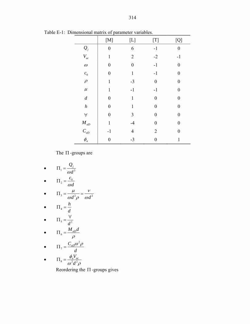
314

Table E-1: Dimensional matrix of parameter variables. [M] [L] [T] [Q]

jQ 0 6 -1 0

acV 1 2 -2 -1

ω 0 0 -1 0

0c 0 1 -1 0 ρ 1 -3 0 0 µ 1 -1 -1 0

d 0 1 0 0

h 0 1 0 0

∀ 0 3 0 0

aDM 1 -4 0 0

aDC -1 4 2 0

aφ 0 -3 0 1

The Π -groups are

• 1 3jQ

dΠ =

ω

• 02

cd

Π =ω

• 3 2 2d dΠ = =

µ νω ρ ω

• 4hd

Π =

• 5 3d∀

Π =

• 6aDM d

Π =ρ

• 2

7aDC

dΠ =

ω ρ

• 8 2 2a acVd

Π =φω ρ

Reordering the Π -groups gives

315

• 1 1 37 8

1 jQ

d′Π = Π =

Π Π ωd

2aDC ω ρ

2ω 2d ρ j j

a ac a ac d

Q QV d V Q

= =φ ω

, the ratio of the jet to

the driver flow rate

• 2 5 4 32

1d∀′Π = Π Π =

Π

2 2h ddω

2

22 2 20 0

1 H

H

hc d c

∝

∀= ∝

ω

ωωω

, the ratio of the operating

frequency to the Helmholtz frequency of the device

• 2

33

1 d S′Π = = =Π

ων

, the Stokes number, i.e. the ratio of the orifice diameter to

the unsteady boundary layer thickness in the orifice

• 4 4hd

′Π = Π = , the orifice ratio

• ( )2 22 237 2 0 0

55

aD aDaD

aC

C c c Cd Cd d Cω ρ ρ

ωΠ Π ⎛ ⎞′Π = = = = =⎜ ⎟Π ∀ ∀⎝ ⎠

C , the ratio between the

compliances of the system

• 7 26 3 4 2 4

6

aD aN

aD aD aD

C Rh hM d d d d M d R

ω ρρ ν µω

Π′Π = Π Π = = =Π

R , the ratio of the

resistances in the system

• 2

27 6 7

aD aDaD aD

d

M d C M Cdω ρ ωω

ρ ω′Π = Π Π = = = , the ratio of the operating

frequency to the natural frequency of the diaphragm

• 2 3

7 88 2 2

5

aD a ac a acC V d Vdd d

Π Π ∆∀′Π = = = ∝Π ∀ ∀ ∀

ω ρ φω ρ

, the ratio of the volume displaced

by the diaphragm to the cavity volume

Thus, the functional equality finally takes the form

, , , , , ,j

d H d

Q hfn SQ d

ω ωω ω

⎛ ⎞ ⎛ ⎞∆∀=⎜ ⎟ ⎜ ⎟∀⎝ ⎠ ⎝ ⎠

C R , (E-4)

316

which is indeed the same as for the generic-driver case given in Chapter 2, with only two

additional terms (the last two ones) that reflect and take into account the piezoelectric-

diaphragm dynamics, while the parameter kd is confined in these two new terms.

Dimensionless Transfer Function

For simplicity, this derivation is for the simple case where only the linear resistance

in the orifice is present ( )0aOnlR = , and where the radiation impedance is neglected

( )0aRadM = since it is usually smaller than aNM .

The transfer function takes the form

( )

( ) 4 3 24 3 2 1 1

j

a aD ac

Q s sC V s a s a s a s a s

=+ + + +φ

, (E-5)

where

( )( )

( )

1

2

3

4

,

,

, and.

aD aN aD aC aN

aD aN aD aC aN aC aD aD aN

aC aD aD aN aN aD

aC aD aD aN

a C R R C R

a C M M C M C C R R

a C C M R M Ra C C M M

= + +⎧⎪

= + + +⎪⎨

= +⎪⎪ =⎩

(E-6)

Substituting the coefficients into the original expression,

( )[ ] [ ]

[ ] [ ]

4 3

2

1...

... 1

j

a aD ac aC aD aD aN aC aD aD aN aC aD aN aD

aD aN aD aD aC aN aC aD aD aN aD aN aD aD aC aN

Q ss C V C C M M s C C M R C C M R s

C M C M C M C C R R s C R C R C R s

=+ + +

+ + + + + + + +

φ (E-7)

or with s jω= ,

( )( ) ( ) ( )

( ) [ ]( )

43

2 2 2 2

22 2

1

...

1 1... 1

j

a aD ac aC aN aD aD

H d d H

aC aN aD aD aD aN aD aN aD aD aC aNd H

Q jj C V j C R C R j

C R C R C M j C R C R C R j

ωω φ ω

ωω ω ω ω

ω ωω ω

=⎡ ⎤

+ + +⎢ ⎥⎣ ⎦

⎡ ⎤+ + + + + + + +⎢ ⎥⎣ ⎦

(E-8)

317

since the diaphragm resonant frequency is defined by 1d aD aDM Cω = and the

Helmholtz resonator frequency is 1H aN aCM C=ω .

But for a circular orifice, the acoustic resistance and mass in the orifice are

respectively

( )48

2aN

hRdµ

π= and

( )24

3 2aN

hMdρ

π= . (E-9)

The acoustic cavity compliance is 2aCC cρ= ∀ , and the Helmholtz frequency for a

round orifice geometry is (see Appendix B)

220

axisym.

32

4H

d c

h

πω

⎛ ⎞⎜ ⎟⎝ ⎠=

∀. (E-10)

The piezoelectric-diaphragm parameters are given by the acoustic mass aDM , the

acoustic compliance aDC , and the acoustic resistance 2aD D aD aDR M Cζ= , where Dζ is

the diaphragm damping ratio. Other quantities of interest are defined as

• aN

aD

MM

=M , the ratio of the masses of the system

• aD

aC

CC

=C , the compliance ratio

• aN

aD

RR

=R , the resistance ratio

From these, the identity 2 2d Hω ω=C M is easily verified.

Combining some of those quantities together yields the following relationships

(derived exclusively for a circular orifice):

318

( ) ( ) ( )4 4 22 22 20 0 0

2 2

8 8 3 4 4842 2 3 2

124 ,

aC aN

H

h h hC Rc dd c d c d

S

µ ν ω ν ωρ ω ωπ π π

ωω

⎛ ⎞∀ ∀ ⋅ ∀ ⎛ ⎞= = = ⎜ ⎟⎜ ⎟⎜ ⎟⎝ ⎠⎝ ⎠

=

(E-11)

2 2 2aD DaD aD aD D D aD aD

aD d

MC R C M CC

ζζ ζω

= = = , (E-12)

2aN

aD aN aD aDaD d

MC M C MM ω

= =M , (E-13)

and

2aN DaD aN aD aD

aD d

RC R C RR

ζω

= = R , or 2 224aD aN aC aNH

C R C RSω

ω= =C C . (E-14)

Thus,

2 2

2 2

24 12 122

aN dH

aD D D D H H D d

R SR S S

ωω ω ω ωζ ω ζ ω ω ζ ω

= = = =C C M

R . (E-15)

By substituting these results into Eq. E-8, the dimensionless form of the transfer

function becomes

( )( ) ( ) ( )

( ) ( )

43

2 2 2 2 2 2

22 2 2 2 2 2 2

1

1 1 124 2 ...

1 1 1 1... 24 2 2 2 24 1

j

a ac D

dH d d H H

D D D

d d dd H H D H

Q jj d V j

jS

j jS S

ωω ω ζω ω

ωω ω ω ω ω

ζ ζ ζω ωω ωω ω ωω ω ω ω ω

=⎡ ⎤

+ + +⎢ ⎥⎣ ⎦

⎡ ⎤ ⎡ ⎤+ + + + + + + +⎢ ⎥ ⎢ ⎥

⎣ ⎦⎣ ⎦

MR

(E-16)

and rearranging term by term,

( )3 34 4 2 2 2

2 2 2 2 2 2 2 2 2 2 2

2

2 2

12 4824 ...

2 24... 2 1

j

D Da ac

H d H d d H d H d H d

D D

d nD H

Q jj d V j j

S S

j j jS

ωζ ω ζ ωω ω ω ω ωω

ω ω ω ω ω ω ω ω ω ω ω

ζ ω ζ ω ωω ω ω

=− − − − − − +

+ + + +

C

R

(E-17)

319

or,

( )

342

2 2 2 2 2 2

34 2

2 2 2 2 2 2

148 1 1 1 ...

2 224 24... 1

j

d D

H d d H H d

D D

H d d H H d

QQ

S

jS S

ζ ωω ωω ω ω ω ω ω

ζ ω ζ ωω ωω ω ω ω ω ω

=⎡ ⎤⎛ ⎞+

− − + + +⎢ ⎥⎜ ⎟⎝ ⎠⎣ ⎦

⎡ ⎤+ − − + + +⎢ ⎥

⎣ ⎦

M

R

(E-18)

where the driver volume flow rate is defined by d a acQ j d Vω= .

At last, one can obtain the final dimensionless expression when dealing with a

circular orifice:

[ ]

[ ]

22 2

2 2 2

22

2 2 2

1

481 1 1 ...

24 24... 2 2 1

j

dD

H d d d

D DH d d d

QQ

S

jS S

ζω ω ω ωω ω ω ω

ω ω ω ωζ ζω ω ω ω

=⎧ ⎫⎡ ⎤⎛ ⎞ ⎛ ⎞⎪ ⎪⎢ ⎥− − + − + + +⎨ ⎬⎜ ⎟ ⎜ ⎟

⎢ ⎥⎝ ⎠ ⎝ ⎠⎪ ⎪⎣ ⎦⎩ ⎭

⎧ ⎫⎡ ⎤⎛ ⎞ ⎛ ⎞⎪ ⎪⎢ ⎥+ − − + +⎨ ⎬⎜ ⎟ ⎜ ⎟⎢ ⎥⎝ ⎠ ⎝ ⎠⎪ ⎪⎣ ⎦⎩ ⎭

M

R

(E-19)

which is indeed a function of the dimensionless numbers Hω ω , dω ω , S , M , and R .

Rectangular Slot

Nondimensional Analysis

For a rectangular orifice, the only change is found in the orifice impedance where

now the acoustic resistance and mass in the orifice are respectively

( )3

32 2

aNhR

w d=

µ and ( )

35 2aN

hMw d

=ρ . (E-20)

Notice the addition of the length scale w which is the spanwise length of the orifice.

From a straightforward dimensional analysis, it is clear that the derivation above for the

case of a circular orifice to obtain the non-dimensional Π -groups will be exactly the

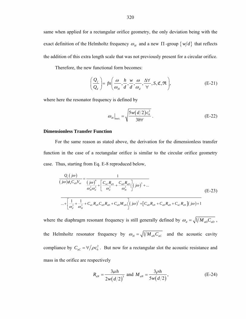
320

same when applied for a rectangular orifice geometry, the only deviation being with the

exact definition of the Helmholtz frequency Hω and a new Π -group w d that reflects

the addition of this extra length scale that was not previously present for a circular orifice.

Therefore, the new functional form becomes:

, , , , , , ,j

d H d

Q h wfn SQ d d

ω ωω ω

⎛ ⎞ ⎛ ⎞∆∀=⎜ ⎟ ⎜ ⎟∀⎝ ⎠ ⎝ ⎠

C R , (E-21)

where here the resonator frequency is defined by

( ) 20

rect.

5 23H

w d ch

ω =∀

. (E-22)

Dimensionless Transfer Function

For the same reason as stated above, the derivation for the dimensionless transfer

function in the case of a rectangular orifice is similar to the circular orifice geometry

case. Thus, starting from Eq. E-8 reproduced below,

( )( ) ( ) ( )

( ) [ ]( )

43

2 2 2 2

22 2

1

...

1 1... 1

j

a aD ac aC aN aD aD

H d d H




ωω φ ω

ωω ω ω ω

ω ωω ω

=⎡ ⎤

+ + +⎢ ⎥⎣ ⎦

⎡ ⎤+ + + + + + + +⎢ ⎥⎣ ⎦

(E-23)

where the diaphragm resonant frequency is still generally defined by 1d aD aDM Cω = ,

the Helmholtz resonator frequency by 1H aN aCM C=ω and the acoustic cavity

compliance by 20aCC cρ= ∀ . But now for a rectangular slot the acoustic resistance and

mass in the orifice are respectively

( )3

32 2

aNhR

w d=

µ and ( )

35 2aN

hMw d

=ρ , (E-24)

321

and the Helmholtz frequency is given by Eq. E-22 when specifically expressed in terms

of the geometric parameters. Again, the piezoelectric-diaphragm parameters are given by

the acoustic mass aDM , the acoustic compliance aDC , and the acoustic resistance

2aD D aD aDR M Cζ= , where Dζ is the diaphragm mechanical damping ratio. Similarly,

other quantities of interest are the ratio of the masses of the system aN aDM M=M , the

compliance ratio aD aCC C=C , and the resistance ratio aN aDR R=R .

Combining some of those quantities together yields the following relationships

(now derived exclusively for a rectangular slot):

( ) ( ) ( )

22

3 32 2 220 00

11

2 2

3 3 5 4 33 2 5 22 2 2 2

110 ,

H

aC aN

S

H

h h hC Rc c w d dw d c w d

S

ω

µ ν ω ν ωρ ω ω

ωω

⎛ ⎞∀ ∀ 3⋅ ∀ ⎛ ⎞= = = ⎜ ⎟⎜ ⎟⎜ ⎟⎝ ⎠⎝ ⎠

=

(E-25)


aD d

MC R C M CC

ζζ ζω

= = = , (E-26)

2aN

aD aN aD aDaD d

MC M C MM ω

= =M , (E-27)

and

2aN DaD aN aD aD

aD d

RC R C RR

ζω

= = R , or 2 210aD aN aD aNH

C R C RSω

ω= =C C . (E-28)

Thus,

2 2

2 2

10 5 52

aN dH

aD D d D H H D d

R SR S S

ωω ω ω ωζ ω ζ ω ω ζ ω

= = =C C M

R . (E-29)

By substituting these results above, the dimensionless form of the transfer function

given by Eq. E-23 becomes

322

( )( ) ( ) ( )

( ) ( )

43

2 2 2 2 2 2

22 2 2 2 2 2 2

1

1 1 110 2 ...

2 21 1 10 10... 2 1

j

a ac D

dH d nD H H

D D D

d d dnD H H d H

Q jj d V j

jS

j jS S

ωω ω ζω ω

ωω ω ω ω ω

ζ ζ ζω ωω ωω ω ωω ω ω ω ω

=⎡ ⎤

+ + +⎢ ⎥⎣ ⎦

⎡ ⎤ ⎡ ⎤+ + + + + + + +⎢ ⎥ ⎢ ⎥

⎣ ⎦⎣ ⎦

MR

(E-30)

and rearranging term by term,

( )3 34 4 2 2 2

2 2 2 2 2 2 2 2 2 2 2

2

2 2

12 2010 ...

2 10... 2 1

j

D Da ac


D D

d d H

Q jj d V j j

S S

j j jS

ωζ ω ζ ωω ω ω ω ωω


ζ ω ζ ω ωω ω ω

=− − − − − − +

+ + + +

M

R

(E-31)

or,

( )

342

2 2 2 2 2 2

34 2

2 2 2 2 2 2

120 1 1 1 ...

2 210 10... 1

j

d D

H d d H H d

D D

H d d H H d

QQ

S

jS S

ζ ωω ωω ω ω ω ω ω

ζ ω ζ ωω ωω ω ω ω ω ω

=⎡ ⎤⎛ ⎞+

− − + + +⎢ ⎥⎜ ⎟⎝ ⎠⎣ ⎦

⎡ ⎤+ − − + + +⎢ ⎥

⎣ ⎦

M

R

(E-32)

where the driver volume flow rate is defined by d a acQ j d Vω= .

At last, one can obtain the final dimensionless expression

[ ]

[ ]

22 2

2 2 2

22

2 2 2

1

201 1 1 ...

10 10... 2 2 1

j

dD

H d d d

D DH d d d

QQ

S

jS S

ζω ω ω ωω ω ω ω

ω ω ω ωζ ζω ω ω ω

=⎧ ⎫⎡ ⎤⎛ ⎞ ⎛ ⎞⎪ ⎪⎢ ⎥− − + − + + +⎨ ⎬⎜ ⎟ ⎜ ⎟

⎢ ⎥⎝ ⎠ ⎝ ⎠⎪ ⎪⎣ ⎦⎩ ⎭

⎧ ⎫⎡ ⎤⎛ ⎞ ⎛ ⎞⎪ ⎪⎢ ⎥+ − − + +⎨ ⎬⎜ ⎟ ⎜ ⎟⎢ ⎥⎝ ⎠ ⎝ ⎠⎪ ⎪⎣ ⎦⎩ ⎭

M

R

(E-33)

which is indeed a function of the dimensionless numbers Hω ω , dω ω , S , M , and R .

323

It is instructive to note that the main difference between the expressions derived for

a circular orifice and a rectangular slot lie exclusively in a constant in front of the square

root of the Stokes number. This critical information allows us to seek a more general

expression that will enclose both geometries, as discussed below.

General Orifice Geometry

The non-dimensional analysis will not be taken here for the general case, since it

has already been shown (see Chapter 2) that the introduction of generic length scale in

lieu of the diameter and of the width and length for respectively the circular and

rectangular orifice geometries is insufficient to collapse the Π -groups into an unified

format. The analysis of the dimensionless transfer function for the general orifice

geometry is however of interest, as shown here.

For simplicity, this derivation is for the simple case where only the linear resistance

in the orifice is present and where the radiation impedance is not taken into account.

As previously demonstrated, the following expression for the transfer function is

easily obtained (see Eq. E-8):

( )( ) ( ) ( )

( ) [ ]( )

43

2 2 2 2

22 2

1

...

1 1... 1

j

a aD ac aC aN aD aD

H d d H




ωω φ ω

ωω ω ω ω

ω ωω ω

=⎡ ⎤

+ + +⎢ ⎥⎣ ⎦

⎡ ⎤+ + + + + + + +⎢ ⎥⎣ ⎦

(E-34)

By combining some of the lumped parameters together in their most general form

and by not expressing those in terms of the geometric parameters (which depend of the

orifice geometry) yield to the following relationships:

2 2 2aNaC aN aC aN aC

aC H

MC R C M CC

ζζ ζω

= = = , (E-35)

324


aD d

MC R C M CC

ζζ ζω

= = = , (E-36)

2aN

aD aN aD aDaD d

MC M C MM ω

= =M , (E-37)

and

2aN DaD aN aD aD

aD d

RC R C RR

ζω

= = R , (E-38)

or

2aD aN aD aNH

C R C R ζω

= =C C (E-39)

Thus,

d

D H

ωζζ ω

=R . (E-40)

Substituting these results above, the dimensionless form of the transfer function,

Eq. E-34, becomes

( )( ) ( ) ( ) ( )

( )

43 2

2 2 2 2 2 2 2

1

1 1 1 12 2 2 2 ...

... 2 2 2 1

j

a ac D D

H d H dH d d H d H d

d D D

D H d d H

Q jj d V j

j j

j

ωω ω ζ ζζ ζω ω

ω ω ω ωω ω ω ω ω ω ω

ω ζ ζζ ζ ωζ ω ω ω ω

=⎡ ⎤ ⎡ ⎤

+ + + + + + +⎢ ⎥ ⎢ ⎥⎣ ⎦ ⎣ ⎦

⎡ ⎤+ + + +⎢ ⎥⎣ ⎦

M

(E-41)

and rearranging terms by terms,

( )3 24 3 2 2 2

2 2 2 2 2 2 2

12 42 ...

2... 2 2 1

j

D Da ac


D

H d H

Q jj d V j j

j j j

ωζ ω ζζ ωω ζω ω ω ωω


ζ ωζω ζωω ω ω

=− − − − − − +

+ + + +

M

(E-42)

325

or,

242

2 2 2 2

33

2 2

14 1 1 1 ...

2 22 4...

j

d D

H d d H H d

D D

H d d H H d

QQ

j

ζζ ωω ωω ω ω ω ω ω

ζ ω ζ ωζω ζωω ω ω ω ω ω

=⎡ ⎤⎛ ⎞+

− − + + +⎢ ⎥⎜ ⎟⎝ ⎠⎣ ⎦

⎡ ⎤+ − − + +⎢ ⎥

⎣ ⎦

M

(E-43)

where the driver volume flow rate is again defined by d a acQ j d V= ω .

At last, one can obtain the final dimensionless expression:

[ ]22 2

2 2

2

1

1 4 1 1 ...

... 2 2 2 2

j

d

DH d H d d

D DH H d d d

QQ

j

ω ω ω ω ωζζω ω ω ω ω

ω ω ω ω ωζ ζ ζω ω ω ω ω

=⎧ ⎫⎡ ⎤⎛ ⎞ ⎛ ⎞⎛ ⎞⎪ ⎪⎢ ⎥− − − + + +⎨ ⎬⎜ ⎟ ⎜ ⎟⎜ ⎟

⎢ ⎥ ⎝ ⎠⎝ ⎠ ⎝ ⎠⎪ ⎪⎣ ⎦⎩ ⎭

⎧ ⎫⎡ ⎤⎡ ⎤⎛ ⎞ ⎛ ⎞⎛ ⎞⎪ ⎪⎢ ⎥⎢ ⎥+ + − +⎨ ⎬⎜ ⎟ ⎜ ⎟⎜ ⎟⎢ ⎥⎢ ⎥⎝ ⎠⎝ ⎠ ⎝ ⎠⎪ ⎪⎣ ⎦⎣ ⎦⎩ ⎭

M

(E-44)

which is indeed a function of the dimensionless numbers Hω ω , dω ω , S , M , and R ,

with the relationship Dζ ζ =R MC , as found in the nondimensional analysis.

Eq. E-44 can be rewritten by frequency power groups to yield

4 22 2 2 2 2

32 2

141 1 1 1 ...

2 22 4...

j

d D

H d H d H d d

D D

H d H d H d

QQ

j

ζζω ωω ω ω ω ω ω ω

ζ ζζ ζω ωω ω ω ω ω ω

=⎧ ⎫⎡ ⎤ ⎡ ⎤⎪ ⎪− + + + + +⎨ ⎬⎢ ⎥ ⎢ ⎥⎪ ⎪⎣ ⎦ ⎣ ⎦⎩ ⎭

⎧ ⎫⎡ ⎤ ⎡ ⎤⎪ ⎪− + − +⎨ ⎬⎢ ⎥ ⎢ ⎥⎪ ⎪⎣ ⎦ ⎣ ⎦⎩ ⎭

M

(E-45)

Thus, a general orifice geometry form of the dimensionless transfer function has

been successively found and expressed in terms of the principal nondimensional

parameters.

326

APPENDIX F

NUMERICAL METHODOLOGY

This section provides background on the numerical scheme employed to simulate

the test cases outlined in Chapter 5. This work has been performed at the George

Washington University under the guidance of Dr. Mittal, and is reproduced here with

permission. First, the numerical scheme employed is discussed in details, and then the

implementation details are described.

VICAR3D, a Cartesian grid solver based on immersed boundary method is used for

simulating the flow inside and outside the ZNMF actuators. The incompressible Navier-

Stokes equations, is written in tensor form as

210;

Rei ji i i

i j i j j

u uu u upx t x x x x

∂∂ ∂ ∂∂= + = − +

∂ ∂ ∂ ∂ ∂ ∂ (F-1)

where the indices 1,2,3i = represent the x, y and z directions, respectively; while the

velocity components are denoted by ( )1for u u , ( )2for v u , and ( )3for w u , respectively.

The equations are non-dimensionalized with the appropriate length and velocity scales

where Re represents the Reynolds number. The Navier-Stokes equations are discretized

using a cell-centered, collocated (non-staggered) arrangement of the primitive variables

( ),u p . In addition to the cell-center velocities ( )u , the face-center velocities U , are

computed. Similar to a fully staggered arrangement, only the component normal to the

cell-face is calculated and stored. The face-center velocity is used for computing the

volume flux from each cell. The advantage of separately computing the face-center

327

velocities has been initially proposed by Zang et al. (1994) and discussed in the context

of the current method by Ye et al. (1999). The equations are integrated in time using the

fractional step method. In the first step, the momentum equations without the pressure

gradient terms are first advanced in time. In a second step, the pressure field is computed

by solving a Poisson equation. A second-order Adams-Bashforth scheme is employed

for the convective terms while the diffusion terms are discretized using an implicit

Crank-Nicolson scheme that eliminates the viscous stability constraint. The pressure

Poisson equation is solved with a Krylov-based approach.

A multi-dimensional ghost-cell methodology is used to incorporate the effect of the

immersed boundary on the flow. The schematic in Figure F-1A shows a solid body with

a curved boundary moving through a fluid, illustrating the current typical flow breadth of

problem of interest (Ghias et al. 2004). The general framework can be considered as

Eulerian-Lagrangian, wherein the immersed boundaries are explicitly tracked as surfaces

in a Lagrangian mode, while the flow computations are performed on a fixed Eulerian

mesh. Hence, we identify cells that are just inside the immersed boundaries as “ghost

cells”. The discrete equations for these cells are then formulated as to satisfy the imposed

boundary condition on the nearby flow boundary to second-order accuracy. These

equations are then solved in a fully coupled manner with the governing flow equations of

the regular fluid cells. Care has been taken to ensure that the equations for the ghost cells

satisfy local and global mass conservation constraints as well as pressure-velocity

compatibility relations. The solver has been designed to take geometrical input from

conventional CAD program. The code has been well validated by comparisons against

established experimental and computational data (Najjar and Mittal 2003).

328

Figure F-1: Schematic of A) the sharp-interface method on a fixed Cartesian mesh, and

B) the ZNMF actuator interacting with a grazing flow. (Reproduced with permission from Dr. Mittal)

Next, the implementation details are described. The typical 3D setup for a

rectangular ZNMF actuator in grazing flows is shown in Figure F-1B. The rectangular

cavity is defined by the width ( )1W , depth ( )2W , and height ( )H . A slot type is chosen

for the jet and is characterized by the width ( )d , height ( )h , and span ( )w . Fluid is

periodically expelled and entrained from and into the cavity by the oscillation of the

diaphragm characterized by the deflection amplitude ( )0W and angular frequency ( )dω .

For the numerical simulations, a pulsatile boundary condition instead of a moving

diaphragm is provided at the bottom of the cavity, ( )0 sin dv W tω= , is provided in order

to generate a flow at the slot exit. The geometrical and the flow parameters are chosen

based on a scaling analysis of various parameters, including the jet Reynolds number

Re invj jV d ν= , and Stokes number 2S dω ν= , where, 0 1 22inv

jW WWV

wdπ= is the average

Jet Exit

U∞

Inflow

h

d

W1

W2

H

Vibrating Diaphragm

w

A B

329

inviscid jet exit velocity and is strictly equal to jV for an incompressible flow. The rest

of the parameters are computed based on the ratios of h d and 1W d .

Figure F-2: Typical mesh used for the computations. A) 2D simulation. B) 3D simulation. (Reproduced with permission from Dr. Mittal)

Figure F-3: Example of 2D and 3D numerical results of ZNMF interacting with a grazing boundary layer. A) Vorticity contours for 2D grazing flow. B) Iso-surface of the vorticity for 3D grazing flow over a circular orifice. (Reproduced with permission from Dr. Mittal)

A B

A B

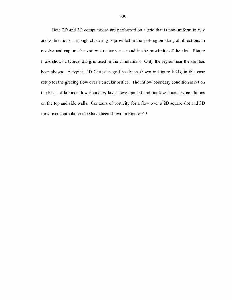
330

Both 2D and 3D computations are performed on a grid that is non-uniform in x, y

and z directions. Enough clustering is provided in the slot-region along all directions to

resolve and capture the vortex structures near and in the proximity of the slot. Figure

F-2A shows a typical 2D grid used in the simulations. Only the region near the slot has

been shown. A typical 3D Cartesian grid has been shown in Figure F-2B, in this case

setup for the grazing flow over a circular orifice. The inflow boundary condition is set on

the basis of laminar flow boundary layer development and outflow boundary conditions

on the top and side walls. Contours of vorticity for a flow over a 2D square slot and 3D

flow over a circular orifice have been shown in Figure F-3.

331

APPENDIX G

EXPERIMENTAL RESULTS: POWER ANALYSIS

This appendix presents the experimental results of the Fourier series decomposition

performed on the phase-locked measurements described in Chapter 3. Table G-1

summarizes the percentage power contained in the fundamental and each harmonic along

with the corresponding square of the residual norm. For each experimental test case, the

percentage of power present at the fundamental frequency and the subsequent harmonics

(up to the 8th harmonic) is listed for Q, the jet volume flow rate, and Mic 1 and Mic 2, the

pressure signals recorded by the microphone 1 and microphone 2, respectively. Here, the

percentage value is computed from

( )%100

PowerPowerMSV

=×

(G-1)

where MSV stands for Mean Square Value. Also given is the corresponding square of the

residual norm 2R coming from the Fourier series decomposition “fit” at each harmonic.

Then, the magnitude (in m3/s for the jet volume flow rate and in Pascal for the pressures)

and phase (in degree) are similarly listed. Finally, the first column of data corresponds to

the total power present in the time series, or the MSV of the residuals.

332

Table G-1: Power in the experimental time data. funda-mental harmonics

case

Total Power

or MSV k = 1 k = 2 k = 3 k = 4 k = 5 k = 6 k = 7 k = 8

Q 6.52E-32 99.40 99.75 99.76 99.77 99.77 99.77 99.77 99.77 Power (%) Mic 1 2.42E-02 99.72 99.74 99.74 99.74 99.75 99.75 99.75 99.75

Q 2.07E-14 3.66E-15 5.40E-16 4.34E-16 4.14E-16 4.13E-16 4.07E-16 4.07E-16 3.89E-16 2R

Mic 1 4.73E-03 1.30E-03 1.22E-03 1.21E-03 1.20E-03 1.17E-03 1.16E-03 1.16E-03 1.16E-03

Q 2.03E-07 1.20E-08 2.43E-09 -1.09E-09 -2.39E-10 -5.89E-10 -1.60E-11 9.90E-10 Magnitude (m3/s) (Pa) Mic 1 0.097 -0.001 0.000 -0.001 0.001 0.000 0.000 0.000

Q 1.43 0.27 0.00 0.08 0.00 0.00 0.00 0.00

9

Phase (o) Mic 1 -0.31 -0.33 -1.00 -0.60 -0.62 -1.09 -1.01 -1.21

Q 9.07E-32 99.26 99.70 99.71 99.71 99.71 99.71 99.71 99.71 Power (%) Mic 1 1.09E-04 99.87 99.88 99.89 99.90 99.90 99.91 99.91 99.91

Q 3.81E-14 8.48E-15 9.52E-16 7.77E-16 7.72E-16 7.13E-16 7.04E-16 6.94E-16 6.93E-16 2R

Mic 1 8.36E-03 1.11E-03 9.90E-04 8.76E-04 8.64E-04 7.93E-04 7.85E-04 7.84E-04 7.66E-04

Q 2.75E-07 1.83E-08 1.69E-09 5.32E-10 -1.80E-09 -7.19E-10 7.12E-10 2.53E-10 Magnitude (m3/s) (Pa) Mic 1 0.129 -0.002 -0.002 0.000 0.001 0.000 0.000 0.001

Q 1.44 0.42 0.48 0.00 0.00 0.00 0.04 -0.02

10

Phase (o) Mic 1 -0.40 -0.45 1.14 -10.94 -1.18 1.13 0.10 0.96

Q 6.74E-33 98.72 99.96 99.96 99.97 99.97 99.97 99.97 99.97 Power (%) Mic 1 1.58E-03 99.75 99.77 99.93 99.93 99.94 99.94 99.95 99.95

Q 1.28E-13 5.90E-14 1.24E-15 9.64E-16 7.80E-16 7.30E-16 7.27E-16 7.12E-16 7.09E-16 2R

Mic 1 2.75E-02 6.75E-03 6.26E-03 1.95E-03 1.89E-03 1.53E-03 1.52E-03 1.46E-03 1.41E-03

Q 5.03E-07 5.63E-08 3.21E-09 -3.43E-09 -1.81E-09 3.71E-10 8.11E-10 4.56E-10 Magnitude (m3/s) (Pa) Mic 1 0.234 -0.003 -0.009 -0.001 0.003 -0.001 -0.001 0.001

Q 1.45 0.64 0.24 0.09 -0.09 0.02 0.09 -0.01

11

Phase (o) Mic 1 -0.49 -0.42 0.43 -1.20 -0.55 -1.34 0.44 1.47

Q 1.55E-31 98.51 99.95 99.95 99.96 99.96 99.96 99.96 99.96 Power (%) Mic 1 4.95E-02 99.36 99.39 99.93 99.93 99.95 99.95 99.95 99.96

Q 2.73E-13 1.45E-13 3.88E-15 3.84E-15 2.04E-15 2.01E-15 1.98E-15 1.97E-15 1.95E-15 2R

Mic 1 5.85E-02 3.71E-02 3.56E-02 4.11E-03 3.84E-03 3.10E-03 3.03E-03 2.68E-03 2.60E-03

Q 7.33E-07 8.86E-08 4.09E-10 -5.92E-09 -1.39E-09 -1.28E-09 -6.51E-10 -1.08E-09 Magnitude (m3/s) (Pa) Mic 1 0.341 -0.005 -0.025 -0.002 0.004 -0.001 -0.003 0.001

Q 1.47 0.77 0.45 -0.20 0.05 0.01 -0.04 0.00

12

Phase (o) Mic 1 -0.55 -0.22 0.72 -1.16 0.12 -1.13 0.78 1.55

Q 6.32E-31 98.48 99.93 99.93 99.95 99.96 99.96 99.96 99.96 Power (%) Mic 1 9.27E-03 98.46 98.57 99.92 99.94 99.95 99.95 99.95 99.95

Q 3.95E-13 2.17E-13 8.59E-15 8.50E-15 3.18E-15 2.79E-15 2.79E-15 2.75E-15 2.74E-15 2R

Mic 1 9.70E-02 1.46E-01 1.36E-01 7.51E-03 5.34E-03 5.21E-03 4.90E-03 4.63E-03 4.47E-03

Q 8.83E-07 1.07E-07 -2.23E-09 -1.26E-08 -4.12E-09 -1.16E-09 -1.72E-09 -3.36E-10 Magnitude (m3/s) (Pa) Mic 1 0.437 -0.014 -0.051 -0.007 0.002 -0.003 -0.002 -0.002

Q 1.48 0.84 0.17 -0.98 -0.43 -0.19 -0.06 -0.02

13

Phase (o) Mic 1 -0.53 -0.07 1.17 -0.91 -0.11 -0.82 1.19 -0.41

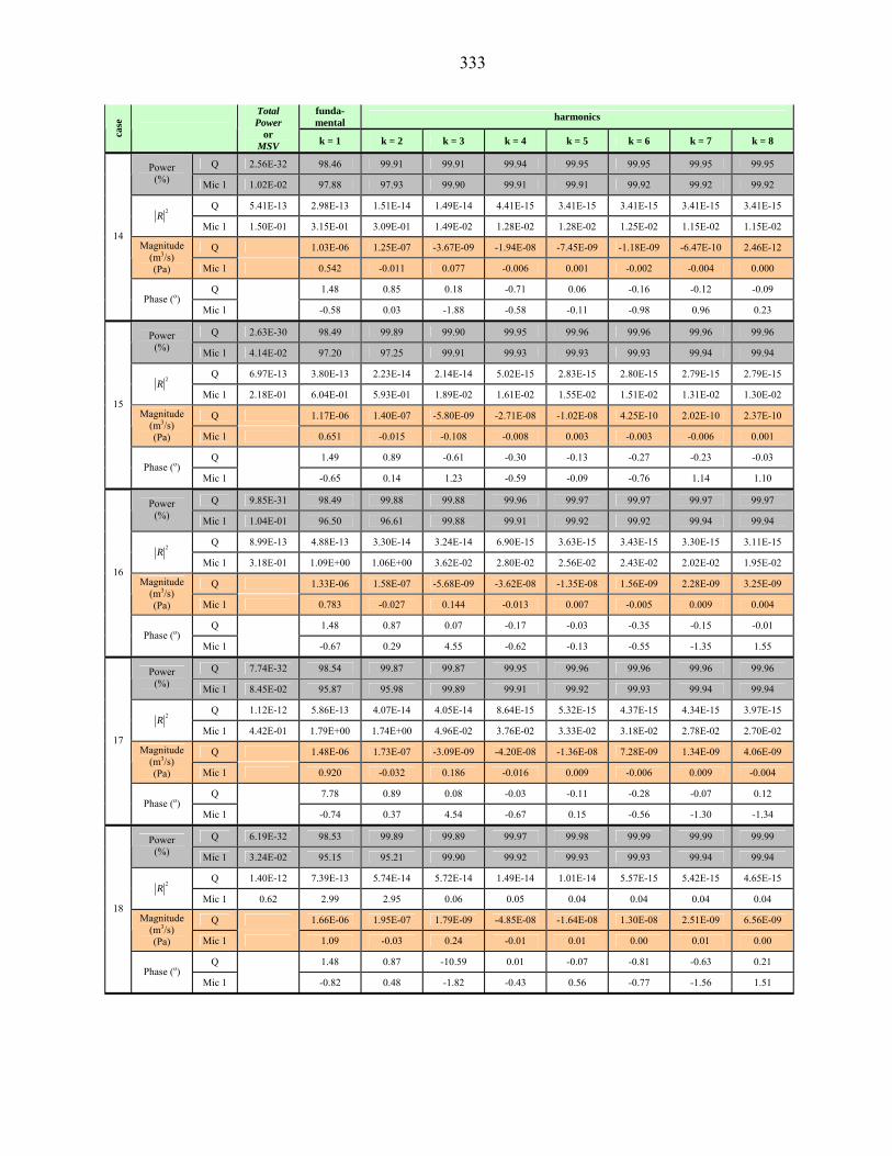
333

funda-mental harmonics

case

Total Power

or MSV k = 1 k = 2 k = 3 k = 4 k = 5 k = 6 k = 7 k = 8

Q 2.56E-32 98.46 99.91 99.91 99.94 99.95 99.95 99.95 99.95 Power (%) Mic 1 1.02E-02 97.88 97.93 99.90 99.91 99.91 99.92 99.92 99.92

Q 5.41E-13 2.98E-13 1.51E-14 1.49E-14 4.41E-15 3.41E-15 3.41E-15 3.41E-15 3.41E-15 2R

Mic 1 1.50E-01 3.15E-01 3.09E-01 1.49E-02 1.28E-02 1.28E-02 1.25E-02 1.15E-02 1.15E-02

Q 1.03E-06 1.25E-07 -3.67E-09 -1.94E-08 -7.45E-09 -1.18E-09 -6.47E-10 2.46E-12 Magnitude (m3/s) (Pa) Mic 1 0.542 -0.011 0.077 -0.006 0.001 -0.002 -0.004 0.000

Q 1.48 0.85 0.18 -0.71 0.06 -0.16 -0.12 -0.09

14

Phase (o) Mic 1 -0.58 0.03 -1.88 -0.58 -0.11 -0.98 0.96 0.23

Q 2.63E-30 98.49 99.89 99.90 99.95 99.96 99.96 99.96 99.96 Power (%) Mic 1 4.14E-02 97.20 97.25 99.91 99.93 99.93 99.93 99.94 99.94

Q 6.97E-13 3.80E-13 2.23E-14 2.14E-14 5.02E-15 2.83E-15 2.80E-15 2.79E-15 2.79E-15 2R

Mic 1 2.18E-01 6.04E-01 5.93E-01 1.89E-02 1.61E-02 1.55E-02 1.51E-02 1.31E-02 1.30E-02

Q 1.17E-06 1.40E-07 -5.80E-09 -2.71E-08 -1.02E-08 4.25E-10 2.02E-10 2.37E-10 Magnitude (m3/s) (Pa) Mic 1 0.651 -0.015 -0.108 -0.008 0.003 -0.003 -0.006 0.001

Q 1.49 0.89 -0.61 -0.30 -0.13 -0.27 -0.23 -0.03

15

Phase (o) Mic 1 -0.65 0.14 1.23 -0.59 -0.09 -0.76 1.14 1.10

Q 9.85E-31 98.49 99.88 99.88 99.96 99.97 99.97 99.97 99.97 Power (%) Mic 1 1.04E-01 96.50 96.61 99.88 99.91 99.92 99.92 99.94 99.94

Q 8.99E-13 4.88E-13 3.30E-14 3.24E-14 6.90E-15 3.63E-15 3.43E-15 3.30E-15 3.11E-15 2R

Mic 1 3.18E-01 1.09E+00 1.06E+00 3.62E-02 2.80E-02 2.56E-02 2.43E-02 2.02E-02 1.95E-02

Q 1.33E-06 1.58E-07 -5.68E-09 -3.62E-08 -1.35E-08 1.56E-09 2.28E-09 3.25E-09 Magnitude (m3/s) (Pa) Mic 1 0.783 -0.027 0.144 -0.013 0.007 -0.005 0.009 0.004

Q 1.48 0.87 0.07 -0.17 -0.03 -0.35 -0.15 -0.01

16

Phase (o) Mic 1 -0.67 0.29 4.55 -0.62 -0.13 -0.55 -1.35 1.55

Q 7.74E-32 98.54 99.87 99.87 99.95 99.96 99.96 99.96 99.96 Power (%) Mic 1 8.45E-02 95.87 95.98 99.89 99.91 99.92 99.93 99.94 99.94

Q 1.12E-12 5.86E-13 4.07E-14 4.05E-14 8.64E-15 5.32E-15 4.37E-15 4.34E-15 3.97E-15 2R

Mic 1 4.42E-01 1.79E+00 1.74E+00 4.96E-02 3.76E-02 3.33E-02 3.18E-02 2.78E-02 2.70E-02

Q 1.48E-06 1.73E-07 -3.09E-09 -4.20E-08 -1.36E-08 7.28E-09 1.34E-09 4.06E-09 Magnitude (m3/s) (Pa) Mic 1 0.920 -0.032 0.186 -0.016 0.009 -0.006 0.009 -0.004

Q 7.78 0.89 0.08 -0.03 -0.11 -0.28 -0.07 0.12

17

Phase (o) Mic 1 -0.74 0.37 4.54 -0.67 0.15 -0.56 -1.30 -1.34

Q 6.19E-32 98.53 99.89 99.89 99.97 99.98 99.99 99.99 99.99 Power (%) Mic 1 3.24E-02 95.15 95.21 99.90 99.92 99.93 99.93 99.94 99.94

Q 1.40E-12 7.39E-13 5.74E-14 5.72E-14 1.49E-14 1.01E-14 5.57E-15 5.42E-15 4.65E-15 2R

Mic 1 0.62 2.99 2.95 0.06 0.05 0.04 0.04 0.04 0.04

Q 1.66E-06 1.95E-07 1.79E-09 -4.85E-08 -1.64E-08 1.30E-08 2.51E-09 6.56E-09 Magnitude (m3/s) (Pa) Mic 1 1.09 -0.03 0.24 -0.01 0.01 0.00 0.01 0.00

Q 1.48 0.87 -10.59 0.01 -0.07 -0.81 -0.63 0.21

18

Phase (o) Mic 1 -0.82 0.48 -1.82 -0.43 0.56 -0.77 -1.56 1.51

334


case

Total Power

or MSV k = 1 k = 2 k = 3 k = 4 k = 5 k = 6 k = 7 k = 8

Q 9.75E-31 98.52 99.89 99.89 99.95 99.97 99.97 99.97 99.97 Power (%) Mic 1 2.37E-02 94.64 94.71 99.91 99.92 99.94 99.94 99.95 99.95

Q 1.72E-12 9.0827E-13

6.5496E-14

6.3768E-14 1.86E-14 1.1727E-

14 8.473E-15 8.162E-15 7.2939E-15 2R

Mic 1 0.86 4.56 4.51 0.08 0.07 0.05 0.05 0.05 0.05

Q 1.84E-06 2.16E-07 9.80E-09 -4.76E-08 -1.93E-08 1.15E-08 3.22E-09 6.94E-09 Magnitude (m3/s) (Pa) Mic 1 1.28 -0.03 0.30 -0.01 0.02 0.00 0.01 0.00

Q 7.78 0.88 0.04 0.21 0.11 -1.00 -1.65 0.25

19

Phase (o) Mic 1 -0.82 0.65 -1.65 -0.16 1.04 -0.51 -1.12 -1.14

Q 2.68E-32 98.55 99.88 99.89 99.95 99.96 99.96 99.96 99.96 Power (%) Mic 1 2.09E-02 94.07 94.14 99.92 99.93 99.95 99.95 99.96 99.96

Q 2.07E-12 1.07E-12 7.96E-14 7.34E-14 2.06E-14 1.30E-14 9.61E-15 9.53E-15 8.43E-15 2R

Mic 1 1.18 6.93 6.85 0.10 0.08 0.06 0.06 0.05 0.05

Q 2.02E-06 2.34E-07 1.79E-08 -4.92E-08 -1.85E-08 1.38E-08 2.13E-09 7.82E-09 Magnitude (m3/s) (Pa) Mic 1 1.49 -0.04 0.37 -0.02 0.02 0.00 0.01 -0.01

Q 1.48 0.83 0.27 0.27 0.13 -0.26 0.05 0.31

20

Phase (o) Mic 1 -0.86 0.70 10.94 -0.17 1.25 -0.67 -0.98 -0.97

Q 5.69E-33 99.71 99.97 99.97 99.98 99.98 99.98 99.98 99.98 Power (%) Mic 1 1.45E-03 99.97 99.98 99.99 99.99 99.99 100 100 100

Q 9.73E-12 1.01E-12 1.04E-13 9.62E-14 5.66E-14 5.54E-14 5.40E-14 5.40E-14 5.37E-14 2R

Mic 1 1171.9 37.66 19.62 12.76 9.49 7.79 6.32 5.38 4.72

Q 4.40E-06 2.24E-07 6.60E-09 4.42E-08 -8.22E-09 8.53E-09 5.58E-10 2.59E-09 Magnitude (m3/s) (Pa) Mic 1 48.41 0.60 0.37 0.26 -0.19 -0.17 -0.14 -0.12

Q -1.82 0.58 -11.71 0.74 0.16 0.03 -1.84 -10.56

21

Phase (o) Mic 1 -0.72 -0.99 -1.08 -1.54 1.34 0.96 0.67 0.29

Q 3.32E-31 98.42 99.94 99.97 99.99 100.00 100.00 100.00 100.00 Power (%) Mic 1 2.05E-03 99.97 99.98 99.99 99.99 99.99 100.00 100.00 100.00

Q 1.67E-11 9.49E-12 3.85E-13 1.75E-13 5.02E-14 2.63E-14 2.40E-14 1.75E-14 1.62E-14 2R

Mic 1 2324.1 70.94 36.45 23.68 16.80 14.36 11.60 9.81 8.53

Q 5.73E-06 7.11E-07 1.08E-07 8.18E-08 -3.87E-08 -1.14E-08 1.87E-08 8.38E-09 Magnitude (m3/s) (Pa) Mic 1 68.17 0.83 0.51 0.37 0.22 0.24 0.19 -0.16

Q -1.81 -0.57 1.10 0.56 -0.45 0.20 -4.41 0.03

22

Phase (o) Mic 1 -0.68 -0.75 -0.73 -1.04 -1.19 -1.35 -1.56 1.27

Q 2.77E-31 98.75 99.95 99.98 99.99 99.99 99.99 100 100 Power (%) Mic 1 8.83E-03 99.98 99.99 99.99 100 100 100 100 100

Q 3.92E-11 1.76E-11 6.59E-13 3.38E-13 1.44E-13 1.41E-13 8.78E-14 4.54E-14 4.04E-14 2R

Mic 1 3396.4 83.46 38.92 24.10 16.63 14.62 11.81 9.80 8.66

Q 8.80E-06 9.71E-07 1.34E-07 1.03E-07 -1.36E-08 -5.41E-08 4.33E-08 1.38E-08 Magnitude (m3/s) (Pa) Mic 1 82.41 0.95 0.55 0.39 0.20 0.24 0.20 0.15

Q -1.94 -0.56 0.96 0.67 0.26 -0.65 -1.49 -0.76

23

Phase (o) Mic 1 -0.67 -0.30 -0.08 0.05 0.49 0.34 0.48 0.60

335


case

Total Power

or MSV k = 1 k = 2 k = 3 k = 4 k = 5 k = 6 k = 7 k = 8

Q 1.10E-31 98.97 99.98 99.99 99.99 99.99 100 100 100 Power (%) Mic 1 5.61E-02 99.92 99.97 99.98 99.99 99.99 99.99 99.99 99.99

Q 7.27E-11 2.69E-11 5.67E-13 3.76E-13 1.48E-13 1.45E-13 1.07E-13 9.13E-14 8.59E-14 2R

Mic 1 4732.9 368.60 160.14 98.31 71.25 60.31 48.97 41.34 36.08

Q 1.20E-05 1.21E-06 1.03E-07 1.13E-07 -1.05E-08 -4.49E-08 2.35E-08 -1.45E-08 Magnitude (m3/s) (Pa) Mic 1 97.23 2.06 1.12 0.74 0.47 0.48 0.39 0.33

Q -1.98 -0.67 1.35 0.59 0.31 -0.19 -1.19 0.72

24

Phase (o) Mic 1 -0.65 -0.13 0.15 0.55 1.08 1.07 1.40 -10.94

Q 0.00E+00 98.93 99.98 99.99 99.99 99.99 100 100 100 Power (%) Mic 1 2.10E-02 99.98 99.99 100 100 100 100 100 100

Q 1.07E-10 4.12E-11 8.73E-13 3.82E-13 2.51E-13 2.51E-13 1.07E-13 7.00E-14 5.82E-14 2R

Mic 1 6399.6 147.03 62.17 29.03 21.64 18.68 13.71 11.76 10.44

Q 1.46E-05 1.50E-06 -1.65E-07 8.46E-08 -2.39E-09 -8.94E-08 4.18E-08 -1.68E-08 Magnitude (m3/s) (Pa) Mic 1 113.11 1.31 0.82 0.39 -0.24 -0.32 -0.20 -0.16

Q -2.02 -0.61 -1.11 0.24 0.05 -0.37 -1.38 0.90

25

Phase (o) Mic 1 -0.59 0.12 0.37 1.13 -0.79 -1.04 -0.56 0.01

Q 5.51E-32 98.97 99.98 99.99 99.99 99.99 100.00 100.00 100.00 Power (%) Mic 1 3.13E-02 99.98 99.99 100.00 100.00 100.00 100.00 100.00 100.00

Q 1.45E-10 5.36E-11 9.35E-13 4.48E-13 3.47E-13 3.28E-13 1.70E-13 9.14E-14 8.82E-14 2R

Mic 1 8181.6 190.01 80.15 27.82 19.29 16.83 13.34 10.95 9.79

Q 1.69E-05 1.71E-06 -1.64E-07 7.50E-08 2.49E-08 -9.33E-08 6.30E-08 -1.22E-08 Magnitude (m3/s) (Pa) Mic 1 127.88 1.49 1.03 0.42 -0.22 -0.27 -0.22 -0.15

Q -2.06 -0.59 -0.69 -0.08 0.95 0.05 -0.70 0.41

26

Phase (o) Mic 1 -0.62 0.13 0.43 1.39 -0.74 -0.72 -0.36 0.46

Q 1.45E-30 98.97 99.97 99.98 99.98 99.98 99.99 100.00 100.00 Power (%) Mic 1 4.10E-02 99.98 99.99 100.00 100.00 100.00 100.00 100.00 100.00

Q 1.76E-10 6.52E-11 1.85E-12 1.59E-12 1.16E-12 1.02E-12 6.27E-13 3.10E-13 2.55E-13 2R

Mic 1 9675.5 243.42 90.32 27.31 18.03 15.07 12.94 9.81 8.96

Q 1.87E-05 1.88E-06 -1.22E-07 1.53E-07 -9.02E-08 -1.47E-07 1.32E-07 5.52E-08 Magnitude (m3/s) (Pa) Mic 1 139.06 1.76 1.13 0.43 -0.24 -0.21 -0.25 -0.13

Q -2.10 -0.65 0.54 0.28 -0.56 0.54 -0.68 -1.25

27

Phase (o) Mic 1 -0.64 0.17 0.52 -10.97 -0.67 -0.72 -0.11 0.84

Q 3.08E-30 98.27 99.74 99.76 99.84 99.90 99.94 99.95 99.97 Power (%) Mic 1 5.58E-02 99.97 99.99 100.00 100.00 100.00 100.00 100.00 100.00

Q 2.26E-10 1.40E-10 2.13E-11 1.96E-11 1.27E-11 8.31E-12 5.15E-12 4.19E-12 2.61E-12 2R

Mic 1 11627 356.00 111.45 29.33 19.73 16.00 12.96 9.08 8.17

Q 2.11E-05 2.57E-06 3.15E-07 6.20E-07 -4.91E-07 -4.19E-07 -2.31E-07 2.96E-07 Magnitude (m3/s) (Pa) Mic 1 152.43 2.22 1.29 0.44 -0.27 -0.25 -0.28 -0.14

Q -2.13 -0.60 0.37 1.10 -0.80 0.01 0.92 -1.69

28

Phase (o) Mic 1 -0.65 0.23 0.62 -4.47 -0.59 -0.78 0.29 1.14

336


case

Total Power

or MSV k = 1 k = 2 k = 3 k = 4 k = 5 k = 6 k = 7 k = 8

Q 4.38E-31 97.12 99.33 99.94 99.97 99.98 99.98 99.98 99.99

Mic 1 8.08E-31 99.99 100.00 100.00 100.00 100.00 100.00 100.00 100.00 Power

(%) Mic 2 4.13E-31 99.97 99.97 99.97 99.98 99.98 100.00 100.00 100.00

Q 7.40E-10 5.12E-10 1.19E-10 1.02E-11 5.19E-12 4.20E-12 3.69E-12 3.25E-12 2.27E-12

Mic 1 15207 151.29 62.58 19.47 14.35 12.21 1.74 1.36 1.29 2R

Mic 2 11260 352.95 292.04 291.33 272.32 257.02 0.91 0.73 0.68

Q 3.79E-05 5.73E-06 -3.01E-06 6.46E-07 2.87E-07 -2.07E-07 -1.90E-07 2.85E-07

Mic 1 174.38 -1.33 -0.93 0.32 -0.21 -0.46 0.09 -0.04 Magnitude

(m3/s) (Pa)

Mic 2 150.05 -1.10 -0.12 -0.62 0.55 2.26 0.06 -0.03

Q 0.33 -0.60 1.10 1.57 -1.31 -0.52 -1.27 1.11

Mic 1 -1.94 0.93 -0.51 -0.34 0.93 -0.29 0.42 0.99

29

Phase (o)

Mic 2 -2.00 1.10 0.76 0.04 -0.02 0.09 4.52 -0.26

Q 4.45E-32 98.39 99.87 99.88 99.93 99.96 99.98 99.98 99.99 Power (%) Mic 1 9.74E-02 99.96 99.99 100.00 100.00 100.00 100.00 100.00 100.00

Q 3.18E-10 1.84E-10 1.47E-11 1.43E-11 7.64E-12 4.56E-12 2.61E-12 1.95E-12 1.10E-12 2R

Mic 1 15538 623.34 154.17 31.21 18.94 14.25 8.36 5.19 4.18

Q -2.50E-05 3.07E-06 1.50E-07 6.09E-07 -4.13E-07 -3.29E-07 -1.92E-07 -2.17E-07 Magnitude (m3/s) (Pa) Mic 1 176.16 3.08 1.58 -0.50 -0.31 -0.34 0.25 0.14

Q 0.95 -0.56 -0.64 0.62 -1.18 -0.52 0.60 1.12

30

Phase (o) Mic 1 -0.58 0.53 1.01 -0.63 -0.24 0.22 -7.74 -0.54

Q 3.48E-31 98.40 99.82 99.84 99.92 99.94 99.97 99.97 99.98 Power (%) Mic 1 1.15E-01 99.95 99.99 100.00 100.00 100.00 100.00 100.00 100.00

Q 3.66E-10 2.11E-10 2.40E-11 2.12E-11 1.10E-11 7.62E-12 4.63E-12 3.44E-12 2.12E-12 2R

Mic 1 17913 821.59 188.88 35.97 23.27 16.08 7.05 3.87 3.10

Q -2.69E-05 3.22E-06 3.92E-07 7.54E-07 4.34E-07 -4.07E-07 -2.57E-07 -2.71E-07 Magnitude (m3/s) (Pa) Mic 1 189.13 3.58 1.76 -0.51 -0.38 -0.43 0.25 0.12

Q 0.91 -0.61 -7.75 0.35 -10.98 -0.78 0.08 0.86

31

Phase (o) Mic 1 -0.59 0.66 1.08 -0.35 -0.09 0.32 -1.09 -0.10

Q 2.03E-30 98.28 99.85 99.86 99.94 99.96 99.97 99.97 99.98 Power (%) Mic 1 1.22E-01 99.95 99.99 100.00 100.00 100.00 100.00 100.00 100.00

Q 4.20E-10 2.60E-10 2.33E-11 2.14E-11 8.72E-12 6.16E-12 4.68E-12 3.87E-12 2.35E-12 2R

Mic 1 20313 1057.70 243.28 44.91 34.51 26.25 7.85 3.95 3.23

Q -2.87E-05 3.63E-06 3.23E-07 8.39E-07 -3.77E-07 -2.86E-07 -2.12E-07 -2.91E-07 Magnitude (m3/s) (Pa) Mic 1 201.38 4.06 2.00 -0.46 -0.41 -0.61 0.28 0.12

Q 0.91 -0.52 -0.91 0.82 -0.71 -0.70 0.06 1.12

32

Phase (o) Mic 1 -0.56893 0.83662 1.1985 -0.093646 0.27526 0.60876 -0.55751 0.30401

Q 4.12E-31 98.44 99.86 99.91 99.95 99.96 99.97 99.98 99.99 Power (%) Mic 1 1.13E-01 99.94 99.98 100.00 100.00 100.00 100.00 100.00 100.00

Q 5.51E-10 3.08E-10 2.77E-11 1.75E-11 9.09E-12 8.84E-12 5.33E-12 3.87E-12 2.25E-12 2R

Mic 1 26230 1621.60 415.32 67.72 61.50 56.03 8.08 4.66 3.90

Q -3.29E-05 3.95E-06 -7.55E-07 6.83E-07 1.16E-07 4.42E-07 -2.85E-07 -3.01E-07

33

Magnitude (m3/s) (Pa) Mic 1 228.84 4.94 2.65 -0.35 -0.33 0.98 0.26 0.12

337


case

Total Power

or MSV k = 1 k = 2 k = 3 k = 4 k = 5 k = 6 k = 7 k = 8

Q 0.86 -0.44 0.72 0.22 0.51 1.51 -0.91 0.10 33 Phase (o)

Mic 1 -0.55 1.16 1.43 -0.16 0.91 -1.62 0.56 1.19

Q 2.24E-30 98.51 99.83 99.92 99.96 99.97 99.98 99.98 99.99 Power (%) Mic 1 1.02E-01 99.93 99.98 100.00 100.00 100.00 100.00 100.00 100.00

Q 6.01E-10 3.23E-10 3.75E-11 1.73E-11 8.15E-12 7.60E-12 4.33E-12 3.47E-12 1.70E-12 2R

Mic 1 29852 2035.60 556.02 91.15 83.75 80.73 10.06 7.37 6.65

Q -3.44E-05 3.98E-06 -1.06E-06 7.14E-07 1.74E-07 4.26E-07 -2.18E-07 -3.14E-07 Magnitude (m3/s) (Pa) Mic 1 244.13 5.47 3.06 -0.39 -0.25 1.19 0.23 0.12

Q 0.85 -0.39 0.65 0.00 -0.05 7.71 -0.96 0.00

34

Phase (o) Mic 1 -0.59 1.22 1.41 -0.71 0.90 -1.44 0.75 1.29

Q 4.32E-31 98.55 99.79 99.93 99.97 99.98 99.99 99.99 99.99 Power (%) Mic 1 8.07E-02 99.93 99.98 100.00 100.00 100.00 100.00 100.00 100.00

Q 6.65E-10 3.47E-10 5.01E-11 1.75E-11 6.46E-12 5.91E-12 3.61E-12 2.86E-12 1.63E-12 2R

Mic 1 33665 2488.30 729.51 120.90 105.48 104.98 9.92 9.26 8.75

Q -3.62E-05 4.06E-06 -1.35E-06 7.82E-07 1.76E-07 3.57E-07 2.04E-07 -2.61E-07 Magnitude (m3/s) (Pa) Mic 1 259.28 5.96 3.51 -0.56 0.10 1.39 -0.11 -0.10

Q 0.83 -0.36 0.55 -0.17 0.02 1.39 -4.51 -0.02

35

Phase (o) Mic 1 -0.58 1.39 1.56 -0.94 1.19 -0.95 -1.31 -1.23

Q 3.79E-30 98.51 99.74 99.93 99.98 99.98 99.99 99.99 99.99 Power (%) Mic 1 2.05E-02 99.93 99.98 100.00 100.00 100.00 100.00 100.00 100.00

Q 7.33E-10 3.92E-10 7.00E-11 1.84E-11 5.90E-12 5.53E-12 3.19E-12 2.89E-12 1.60E-12 2R

Mic 1 38139 2553.10 943.74 168.81 131.76 125.37 14.39 11.26 10.53

Q -3.80E-05 4.23E-06 -1.69E-06 8.34E-07 1.44E-07 3.60E-07 1.29E-07 -2.68E-07 Magnitude (m3/s) (Pa) Mic 1 276.06 5.70 3.96 0.87 0.36 1.50 -0.25 -0.12

Q 0.81 -0.30 0.43 -0.22 -0.25 1.56 1.37 -0.41

36

Phase (o) Mic 1 -0.62 1.59 1.53 7.74 0.13 -0.74 0.59 -0.51

Q 7.71E-31 98.62 99.63 99.93 99.98 99.99 99.99 99.99 99.99 Power (%) Mic 1 5.89E-02 99.91 99.97 100.00 100.00 100.00 100.00 100.00 100.00

Q 7.77E-10 3.87E-10 1.03E-10 2.07E-11 4.72E-12 4.21E-12 2.63E-12 2.34E-12 1.56E-12 2R

Mic 1 41843 3645.00 1421.30 214.02 135.43 134.49 19.24 13.34 13.27

Q -3.91E-05 3.97E-06 -2.14E-06 9.42E-07 1.69E-07 2.96E-07 1.28E-07 -2.07E-07 Magnitude (m3/s) (Pa) Mic 1 289.07 6.74 4.96 1.27 -0.14 1.53 -0.35 -0.04

Q 0.79 -0.27 0.43 -0.47 -0.68 1.40 -0.11 -0.76

37

Phase (o) Mic 1 -0.65 1.41 1.52 -4.55 -1.41 -0.70 1.07 0.42

Q 2.86E-30 98.64 99.55 99.90 99.97 99.98 99.98 99.98 99.99 Power (%) Mic 1 1.81E-03 99.92 99.97 100.00 100.00 100.00 100.00 100.00 100.00

Q 8.36E-10 4.10E-10 1.37E-10 3.12E-11 8.31E-12 7.49E-12 5.57E-12 4.90E-12 3.33E-12 2R

Mic 1 48009 3680.00 1349.70 222.33 175.58 173.36 33.20 21.82 20.66

Q -4.06E-05 3.89E-06 -2.43E-06 1.13E-06 2.14E-07 3.26E-07 1.93E-07 -2.96E-07 Magnitude (m3/s) (Pa) Mic 1 309.75 6.86 4.77 0.97 0.21 1.68 -0.48 -0.15

Q 0.79 -0.28 0.56 -0.36 -1.01 1.13 0.58 -0.97

38

Phase (o) Mic 1 -0.61 1.87 -4.54 -4.55 0.61 -0.11 0.99 0.55

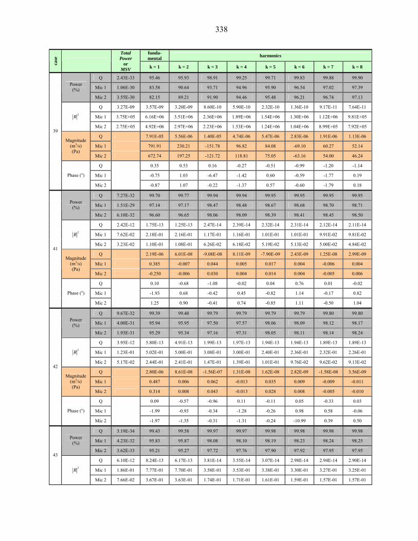
338


case

Total Power

or MSV k = 1 k = 2 k = 3 k = 4 k = 5 k = 6 k = 7 k = 8

Q 2.43E-33 95.46 95.93 98.91 99.25 99.71 99.83 99.88 99.90

Mic 1 1.06E-30 83.58 90.64 93.71 94.96 95.90 96.54 97.02 97.39 Power

(%) Mic 2 3.55E-30 82.15 89.21 91.90 94.46 95.48 96.21 96.74 97.13

Q 3.27E-09 3.57E-09 3.20E-09 8.60E-10 5.90E-10 2.32E-10 1.36E-10 9.17E-11 7.64E-11

Mic 1 3.75E+05 6.16E+06 3.51E+06 2.36E+06 1.89E+06 1.54E+06 1.30E+06 1.12E+06 9.81E+05 2R

Mic 2 2.75E+05 4.92E+06 2.97E+06 2.23E+06 1.53E+06 1.24E+06 1.04E+06 8.99E+05 7.92E+05

Q 7.91E-05 5.56E-06 1.40E-05 4.74E-06 5.47E-06 2.83E-06 1.91E-06 1.13E-06

Mic 1 791.91 230.21 -151.78 96.82 84.08 -69.10 60.27 52.14 Magnitude

(m3/s) (Pa)

Mic 2 672.74 197.25 -121.72 118.81 75.05 -63.16 54.00 46.24

Q 0.35 0.53 0.16 -0.27 -0.51 -0.99 -1.20 -1.14

Mic 1 -0.75 1.03 -6.47 -1.42 0.60 -0.59 -1.77 0.19

39

Phase (o)

Mic 2 -0.87 1.07 -0.22 -1.37 0.57 -0.60 -1.79 0.18

Q 7.27E-32 99.70 99.77 99.94 99.94 99.95 99.95 99.95 99.95

Mic 1 1.51E-29 97.14 97.17 98.47 98.48 98.67 98.68 98.70 98.71 Power

(%) Mic 2 6.10E-32 96.60 96.65 98.06 98.09 98.39 98.41 98.45 98.50

Q 2.42E-12 1.75E-13 1.25E-13 2.47E-14 2.39E-14 2.32E-14 2.31E-14 2.12E-14 2.11E-14

Mic 1 7.62E-02 2.18E-01 2.16E-01 1.17E-01 1.16E-01 1.01E-01 1.01E-01 9.91E-02 9.81E-02 2R

Mic 2 3.23E-02 1.10E-01 1.08E-01 6.26E-02 6.18E-02 5.19E-02 5.13E-02 5.00E-02 4.84E-02

Q 2.19E-06 6.01E-08 -9.08E-08 8.11E-09 -7.90E-09 2.43E-09 1.25E-08 2.99E-09

Mic 1 0.385 -0.007 0.044 0.005 0.017 0.004 -0.006 0.004 Magnitude

(m3/s) (Pa)

Mic 2 -0.250 -0.006 0.030 0.004 0.014 0.004 -0.005 0.006

Q 0.10 -0.68 -1.08 -0.02 0.04 0.76 0.01 -0.02

Mic 1 -1.93 0.68 -0.42 0.45 -0.82 1.14 -0.17 0.82

41

Phase (o)

Mic 2 1.25 0.90 -0.41 0.74 -0.85 1.11 -0.50 1.04

Q 9.67E-32 99.39 99.48 99.79 99.79 99.79 99.79 99.80 99.80

Mic 1 4.00E-31 95.94 95.95 97.50 97.57 98.06 98.09 98.12 98.17 Power

(%) Mic 2 1.93E-31 95.29 95.34 97.16 97.31 98.05 98.11 98.14 98.24

Q 3.95E-12 5.80E-13 4.91E-13 1.99E-13 1.97E-13 1.94E-13 1.94E-13 1.89E-13 1.89E-13

Mic 1 1.23E-01 5.02E-01 5.00E-01 3.08E-01 3.00E-01 2.40E-01 2.36E-01 2.32E-01 2.26E-01 2R

Mic 2 5.17E-02 2.44E-01 2.41E-01 1.47E-01 1.39E-01 1.01E-01 9.76E-02 9.62E-02 9.13E-02

Q 2.80E-06 8.61E-08 -1.56E-07 1.31E-08 1.62E-08 2.82E-09 -1.58E-08 3.56E-09

Mic 1 0.487 0.006 0.062 -0.013 0.035 0.009 -0.009 -0.011 Magnitude

(m3/s) (Pa)

Mic 2 0.314 0.008 0.043 -0.013 0.028 0.008 -0.005 -0.010

Q 0.09 -0.57 -0.96 0.11 -0.11 0.05 -0.33 0.03

Mic 1 -1.99 -0.93 -0.34 -1.28 -0.26 0.98 0.58 -0.06

42

Phase (o)

Mic 2 -1.97 -1.35 -0.31 -1.31 -0.24 -10.99 0.39 0.50

Q 3.19E-34 99.43 99.58 99.97 99.97 99.98 99.98 99.98 99.98

Mic 1 4.23E-32 95.83 95.87 98.08 98.10 98.19 98.23 98.24 98.25 Power

(%) Mic 2 3.62E-33 95.21 95.27 97.72 97.76 97.90 97.92 97.95 97.95

Q 6.10E-12 8.24E-13 6.17E-13 3.81E-14 3.55E-14 3.07E-14 2.98E-14 2.94E-14 2.90E-14

Mic 1 1.86E-01 7.77E-01 7.70E-01 3.58E-01 3.53E-01 3.38E-01 3.30E-01 3.27E-01 3.25E-01

43

2R

Mic 2 7.66E-02 3.67E-01 3.63E-01 1.74E-01 1.71E-01 1.61E-01 1.59E-01 1.57E-01 1.57E-01

339


case

Total Power

or MSV k = 1 k = 2 k = 3 k = 4 k = 5 k = 6 k = 7 k = 8

Q 3.48E-06 1.31E-07 -2.20E-07 1.46E-08 1.91E-08 8.48E-09 -5.88E-09 5.96E-09

Mic 1 0.598 0.012 0.091 -0.010 0.017 -0.013 -0.007 0.007 Magnitude

(m3/s) (Pa)

Mic 2 0.382 0.010 0.061 -0.008 0.014 -0.007 -0.006 -0.001

Q 0.08 -0.51 -0.78 0.06 0.50 -0.03 0.03 0.09

Mic 1 -2.03 -1.35 -0.31 0.72 -0.36 -0.89 0.83 -1.23

43

Phase (o)

Mic 2 -2.00 23.56 -0.33 -0.06 0.15 -1.01 0.62 -0.14

Q 1.03E-32 99.71 99.80 99.95 99.96 100.00 100.00 100.00 100.00

Mic 1 1.06E-30 99.37 99.43 99.98 99.99 99.99 99.99 99.99 99.99 Power

(%) Mic 2 6.75E-32 99.00 99.06 99.99 99.99 100.00 100.00 100.00 100.00

Q 4.83E-09 3.38E-10 2.37E-10 6.38E-11 4.96E-11 5.09E-12 2.98E-12 1.34E-12 1.07E-12

Mic 1 1.13E+04 7.09E+03 6.40E+03 2.05E+02 1.46E+02 8.87E+01 8.30E+01 7.38E+01 6.98E+01 2R

Mic 2 5.06E+03 5.08E+03 4.77E+03 4.40E+01 3.39E+01 2.71E+01 2.69E+01 2.64E+01 2.60E+01

Q 9.82E-05 -2.90E-06 3.80E-06 1.08E-06 1.93E-06 -4.19E-07 3.70E-07 -1.47E-07

Mic 1 149.71 3.72 11.13 -1.08 1.07 0.34 -0.43 -0.28 Magnitude

(m3/s) (Pa)

Mic 2 100.07 2.48 -9.73 -0.45 0.37 0.07 0.10 0.08

Q 0.16 0.97 -1.22 0.22 -0.16 0.81 -0.95 -0.96

Mic 1 -2.10 0.66 2.66 0.58 -0.60 0.56 -0.77 0.80

44

Phase (o)

Mic 2 -2.14 0.42 -0.26 0.11 -0.83 0.59 1.28 -0.68

Q 2.20E-31 98.81 99.04 99.92 99.93 99.97 99.98 99.99 100.00

Mic 1 4.02E-30 98.86 98.90 99.95 99.95 99.96 99.96 99.97 99.97 Power

(%) Mic 2 1.92E-31 98.20 98.20 99.98 99.98 99.98 99.98 99.98 99.98

Q 7.36E-09 2.09E-09 1.70E-09 1.38E-10 1.24E-10 5.42E-11 3.89E-11 1.15E-11 9.04E-12

Mic 1 2.65E+04 3.02E+04 2.93E+04 1.35E+03 1.31E+03 9.91E+02 9.74E+02 9.21E+02 9.00E+02 2R

Mic 2 1.22E+04 2.20E+04 2.19E+04 2.52E+02 2.44E+02 2.22E+02 2.20E+02 2.15E+02 2.15E+02

Q 0.00012062 5.72E-06 1.14E-05 1.08E-06 2.42E-06 1.13E-06 1.51E-06 4.55E-07

Mic 1 229.11 -4.04 23.66 0.95 2.53 -0.59 1.03 0.65 Magnitude

(m3/s) (Pa)

Mic 2 154.66 -1.24 20.81 -0.40 0.66 -0.20 0.30 -0.09

Q 0.36 -1.14 -0.53 1.54 0.86 -0.17 0.36 -0.91

Mic 1 -2.12 -0.38 -40.33 -1.24 1.32 0.48 -0.78 1.06

45

Phase (o)

Mic 2 -2.16 -0.07 -2.55 1.28 1.19 0.56 0.22 0.12

Q 5.43E-31 99.89 99.92 99.92 99.92 99.92 99.92 99.95 99.95

Mic 1 6.87E-32 100.00 100.00 100.00 100.00 100.00 100.00 100.00 100.00 Power

(%) Mic 2 5.27E-32 100.00 100.00 100.00 100.00 100.00 100.00 100.00 100.00

Q 1.96E-11 4.99E-13 3.65E-13 3.58E-13 3.55E-13 3.54E-13 3.46E-13 2.44E-13 2.41E-13

Mic 1 1.84E+02 2.33E-02 2.24E-02 1.03E-02 9.68E-03 8.49E-03 8.28E-03 6.43E-03 6.36E-03 2R

Mic 2 8.63E+01 2.42E-02 1.42E-02 1.03E-02 1.00E-02 7.98E-03 7.87E-03 5.89E-03 5.88E-03

Q 6.26E-06 -1.06E-07 -1.45E-08 9.90E-09 -6.50E-09 -1.72E-08 -9.19E-08 -1.31E-08

Mic 1 19.171 0.004 -0.016 -0.003 0.005 -0.002 -0.006 0.001 Magnitude

(m3/s) (Pa)

Mic 2 13.135 0.014 -0.009 -0.002 0.006 0.001 -0.006 0.000

Q 0.09 0.87 -1.79 1.94 -0.03 1.78 0.57 0.89

Mic 1 -1.63 -0.72 0.82 -1.19 1.20 1.26 1.19 -0.65

46

Phase (o)

Mic 2 -1.63 -0.56 1.03 -1.41 1.29 -1.07 1.17 1.13

340


case

Total Power

or MSV k = 1 k = 2 k = 3 k = 4 k = 5 k = 6 k = 7 k = 8

Q 3.02E-34 99.95 100.00 100.00 100.00 100.00 100.00 100.00 100.00

Mic 1 2.76E-31 100.00 100.00 100.00 100.00 100.00 100.00 100.00 100.00 Power

(%) Mic 2 1.10E-33 100.00 100.00 100.00 100.00 100.00 100.00 100.00 100.00

Q 1.03E-10 1.22E-12 1.07E-13 6.96E-14 1.31E-14 1.26E-14 1.08E-14 1.04E-14 1.02E-14

Mic 1 9.69E+02 1.15E+00 6.61E-02 9.54E-03 7.92E-03 4.41E-03 4.13E-03 4.07E-03 4.02E-03 2R

Mic 2 4.59E+02 1.15E+00 1.43E-02 6.63E-03 5.00E-03 4.42E-03 3.84E-03 3.16E-03 3.12E-03

Q 1.44E-05 -3.05E-07 -5.57E-08 6.57E-08 3.70E-09 7.92E-09 -5.28E-09 -3.40E-09

Mic 1 44.022 -0.147 -0.034 0.006 -0.008 0.002 0.001 -0.001 Magnitude

(m3/s) (Pa)

Mic 2 30.312 -0.151 0.012 -0.006 -0.003 0.003 0.004 -0.001

Q 0.22 0.60 -0.59 0.98 0.54 0.86 0.24 -0.65

Mic 1 -1.62 0.52 -1.19 1.09 -1.05 -1.03 10.96 -0.80

47

Phase (o)

Mic 2 -1.61 0.68 -0.68 -0.80 -1.25 -0.61 -0.76 0.90

Q 2.20E-30 99.96 99.96 99.98 100.00 100.00 100.00 100.00 100.00

Mic 1 6.78E-31 100.00 100.00 100.00 100.00 100.00 100.00 100.00 100.00 Power

(%) Mic 2 5.60E-31 100.00 100.00 100.00 100.00 100.00 100.00 100.00 100.00

Q 5.10E-10 4.68E-12 4.66E-12 2.60E-12 5.44E-13 4.33E-13 2.09E-13 1.67E-13 1.28E-13

Mic 1 4303.2 7.83 2.86 0.67 0.54 0.09 0.03 0.02 0.02 2R

Mic 2 2076.8 5.35 0.82 0.34 0.33 0.23 0.02 0.01 0.01

Q 3.19E-05 -3.00E-08 4.15E-07 4.14E-07 -9.47E-08 -1.37E-07 -5.77E-08 -6.08E-08

Mic 1 92.77 -0.32 0.21 0.05 -0.09 -0.03 0.01 -0.01 Magnitude

(m3/s) (Pa)

Mic 2 64.45 -0.30 0.10 0.02 0.04 -0.06 0.02 0.00

Q 0.15 -0.32 -0.07 -1.54 -0.13 -0.25 -0.90 -0.48

Mic 1 -1.66 0.46 -0.12 0.88 -0.12 -0.07 -0.36 0.76

48

Phase (o)

Mic 2 -1.66 0.53 -1.06 0.88 -0.80 0.99 -4.56 -0.36

Q 2.92E-30 99.59 99.94 99.96 99.98 99.99 99.99 99.99 100.00

Mic 1 0 99.97 99.99 100.00 100.00 100.00 100.00 100.00 100.00 Power

(%) Mic 2 1.55E-30 99.97 100.00 100.00 100.00 100.00 100.00 100.00 100.00

Q 2.54E-09 2.48E-10 3.57E-11 2.42E-11 1.27E-11 6.60E-12 6.05E-12 3.42E-12 1.95E-12

Mic 1 16391 573.63 167.09 7.63 2.70 1.78 0.43 0.17 0.16 2R

Mic 2 8156.4 270.28 8.76 3.66 2.94 2.03 0.68 0.14 0.12

Q 7.11E-05 4.21E-06 9.80E-07 9.78E-07 7.14E-07 2.13E-07 4.68E-07 3.50E-07

Mic 1 181.03 2.85 1.79 0.31 -0.14 -0.16 0.07 -0.02 Magnitude

(m3/s) (Pa)

Mic 2 127.70 2.29 0.32 0.12 -0.13 -0.16 -0.10 -0.02

Q 0.34 -0.52 0.82 -0.05 0.16 0.22 0.62 -0.33

Mic 1 -1.70 -7.74 0.50 1.26 0.14 0.61 1.48 -0.61

49

Phase (o)

Mic 2 -1.74 -1.30 0.32 1.40 0.55 1.26 0.83 -0.53

Q 3.65E-34 99.41 99.93 99.95 99.95 99.99 100.00 100.00 100.00

Mic 1 1.48E-31 99.91 99.97 100.00 100.00 100.00 100.00 100.00 100.00 Power

(%) Mic 2 1.70E-31 99.91 99.99 100.00 100.00 100.00 100.00 100.00 100.00

Q 5.46E-09 7.78E-10 9.82E-11 6.80E-11 6.51E-11 8.82E-12 3.74E-12 1.06E-12 8.27E-13

Mic 1 3.42E+04 3.03E+03 1.17E+03 1.41E+02 1.02E+02 5.08E+01 6.15E+00 1.65E+00 7.09E-01

50

2R

Mic 2 1.71E+04 1.57E+03 1.76E+02 8.13E+01 7.87E+01 7.25E+01 5.05E+00 7.12E-01 4.69E-01

341


case

Total Power

or MSV k = 1 k = 2 k = 3 k = 4 k = 5 k = 6 k = 7 k = 8

Q 0.00010423 7.53E-06 1.59E-06 -4.94E-07 2.17E-06 6.51E-07 4.72E-07 1.40E-07

Mic 1 261.28 6.10 4.53 -0.89 -1.01 0.95 -0.30 0.14 Magnitude

(m3/s) (Pa)

Mic 2 185.11 5.27 1.37 0.23 -0.35 1.16 0.29 0.07

Q 0.27 -0.35 4.56 0.70 0.92 0.03 0.63 10.98

Mic 1 -1.96 -1.41 -4.52 -1.11 1.24 4.49 0.64 -1.03

50

Phase (o)

Mic 2 -2.04 -1.15 -4.53 7.73 -0.17 -0.88 -0.55 -0.66

Q 1.55E-30 99.89 99.89 99.90 99.90 99.90 99.90 99.90 99.90

Mic 1 2.21E-31 98.94 98.96 99.40 99.41 99.44 99.44 99.45 99.46 Power

(%) Mic 2 2.62E-30 36.28 37.31 39.32 41.52 49.46 50.44 50.95 54.68

Q 1.33E-12 3.43E-14 3.18E-14 2.90E-14 2.90E-14 2.88E-14 2.88E-14 2.88E-14 2.88E-14

Mic 1 1.25E-01 1.33E-01 1.31E-01 7.51E-02 7.37E-02 7.05E-02 7.03E-02 6.90E-02 6.81E-02 2R

Mic 2 3.05E-04 1.94E-02 1.91E-02 1.85E-02 1.78E-02 1.54E-02 1.51E-02 1.50E-02 1.38E-02

Q 1.63E-06 -3.85E-09 1.51E-08 -9.51E-10 3.55E-09 1.69E-09 8.04E-10 -1.05E-09

Mic 1 0.50 -0.007 0.033 0.005 0.008 -0.002 -0.005 -0.004 Magnitude

(m3/s) (Pa)

Mic 2 0.015 -0.003 -0.004 0.004 -0.007 0.002 0.002 -0.005

Q 0.04 1.01 0.61 -0.04 -9.91 0.00 -0.01 -0.06

Mic 1 -1.65 -1.15 0.08 -0.69 -0.57 0.53 1.26 0.77

51

Phase (o)

Mic 2 -0.20 0.54 -1.08 -0.76 0.93 -1.51 0.97 1.04

Q 5.41E-31 99.68 99.82 99.96 99.96 99.96 99.96 99.96 99.96

Mic 1 8.52E-31 91.91 91.93 93.33 93.34 93.36 93.36 93.36 93.39 Power

(%) Mic 2 NaN NaN NaN NaN NaN NaN NaN NaN NaN

Q 2.62E-12 2.03E-13 1.11E-13 2.38E-14 2.37E-14 2.33E-14 2.33E-14 2.27E-14 2.27E-14

Mic 1 0.255 2.063 2.059 1.702 1.699 1.695 1.695 1.693 1.685 2R

Mic 2 NaN NaN NaN NaN NaN NaN NaN NaN NaN

Q 2.29E-06 -8.79E-08 -8.44E-08 3.22E-09 4.42E-09 -1.15E-09 -6.13E-09 1.49E-09

Mic 1 0.68 0.009 0.084 -0.008 0.009 0.003 0.006 0.012 Magnitude

(m3/s) (Pa)

Mic 2 NaN NaN NaN NaN NaN NaN NaN NaN

Q 0.01 1.01 -0.98 -0.01 -9.96 -0.01 0.41 -1.94

Mic 1 4.58 1.07 0.27 -0.05 0.25 -0.61 0.99 -0.67

52

Phase (o)


Q 1.16E-30 99.637 99.785 99.994 99.995 99.995 99.995 99.995 99.996

Mic 1 8.92E-31 96.369 96.405 98.784 98.792 98.822 98.823 98.837 98.841 Power


Q 4.5389E-12

3.9586E-13

2.3307E-13

5.8209E-15

5.0713E-15 3.518E-15 3.0998E-

15 2.9485E-

15 2.9023E-

15

Mic 1 0.403 1.463 1.449 0.490 0.487 0.475 0.474 0.469 0.467 2R


Q 3.01E-06 -1.16E-07 -1.38E-07 7.90E-09 6.33E-09 5.42E-09 2.74E-09 1.94E-09

Mic 1 0.88 0.017 0.138 -0.008 0.016 0.003 0.010 0.006 Magnitude

(m3/s) (Pa)


Q 0.01 1.21 -0.90 0.01 0.52 0.15 0.20 -0.03

Mic 1 4.55 0.96 0.28 0.56 0.08 0.70 0.16 1.13

53

Phase (o)


342


case

Total Power

or MSV k = 1 k = 2 k = 3 k = 4 k = 5 k = 6 k = 7 k = 8

Q 4.10E-30 99.49 99.71 99.99 99.99 99.99 100.00 100.00 100.00

Mic 1 7.14E-33 96.29 96.30 98.75 98.76 98.86 98.86 98.88 98.88 Power


Q 7.30E-12 8.96E-13 5.12E-13 1.28E-14 1.00E-14 4.27E-15 3.98E-15 3.76E-15 3.55E-15

Mic 1 0.621 2.304 2.296 0.775 0.768 0.709 0.709 0.696 0.695 2R


Q 3.81E-06 -1.78E-07 -2.04E-07 1.26E-08 2.18E-08 4.58E-09 2.64E-09 4.08E-09

Mic 1 1.09 0.013 0.174 -0.012 0.034 -0.001 0.016 -0.005 Magnitude

(m3/s) (Pa)


Q -0.01 1.12 -0.84 0.86 1.58 0.11 0.30 0.08

Mic 1 -1.78 0.92 0.28 0.21 0.02 -1.41 -0.42 0.42

54

Phase (o)


Q 1.97E-32 99.90 99.91 99.91 99.91 99.92 99.92 99.94 99.94

Mic 1 1.57E-29 100.00 100.00 100.00 100.00 100.00 100.00 100.00 100.00 Power


Q 2.52E-11 6.08E-13 5.55E-13 5.43E-13 5.37E-13 5.01E-13 4.94E-13 3.73E-13 3.67E-13

Mic 1 810.91 0.090 0.090 0.079 0.061 0.060 0.059 0.056 0.054 2R


Q 7.10E-06 -6.44E-08 3.04E-08 2.35E-08 -5.27E-08 2.22E-08 -1.00E-07 2.19E-08

Mic 1 40.27 0.003 0.015 0.019 0.005 0.003 0.008 0.007 Magnitude

(m3/s) (Pa)


Q 0.21 0.21 -0.07 0.00 1.17 -0.59 1.11 -0.28

Mic 1 -1.54 -1.55 -1.56 0.77 -0.18 -1.13 1.56 0.48

55

Phase (o)


Q 4.84E-32 99.57 99.92 99.98 99.98 99.99 99.99 99.99 99.99

Mic 1 3.38E-31 99.94 99.97 99.98 99.99 99.99 99.99 99.99 99.99 Power


Q 1.65E-10 1.70E-11 3.02E-12 8.10E-13 7.19E-13 5.66E-13 5.32E-13 4.66E-13 3.79E-13

Mic 1 4355.4 251.58 116.91 77.59 58.13 47.66 40.05 34.38 30.10 2R


Q 1.81E-05 -1.08E-06 4.29E-07 8.61E-08 1.13E-07 4.85E-08 6.97E-08 8.50E-08

Mic 1 93.31 -1.64 -0.89 0.62 0.46 0.39 -0.34 -0.29 Magnitude

(m3/s) (Pa)


Q 0.03 -0.31 -0.09 -0.90 -1.18 -0.66 -1.16 -1.27

Mic 1 -1.52 0.55 -0.66 1.34 0.12 -1.11 0.82 -0.41

56

Phase (o)


Q 7.30E-32 99.25 99.72 99.83 99.90 99.95 99.97 99.98 99.99

Mic 1 3.30E-32 100.00 100.00 100.00 100.00 100.00 100.00 100.00 100.00 Power

(%) Mic 2 8.63E-33 100.00 100.00 100.00 100.00 100.00 100.00 100.00 100.00

Q 8.25E-10 1.49E-10 5.63E-11 3.44E-11 2.01E-11 1.07E-11 5.95E-12 3.51E-12 1.60E-12

Mic 1 24466 76.48 63.21 3.26 3.23 0.69 0.33 0.31 0.28

57

2R

Mic 2 3744.6 1.58 1.47 0.41 0.36 0.31 0.21 0.18 0.18

343


case

Total Power

or MSV k = 1 k = 2 k = 3 k = 4 k = 5 k = 6 k = 7 k = 8

Q 4.05E-05 -2.78E-06 -1.35E-06 1.09E-06 8.87E-07 6.28E-07 4.51E-07 -3.99E-07

Mic 1 221.20 -0.52 1.09 -0.02 -0.23 0.08 -0.02 0.02 Magnitude

(m3/s) (Pa)

Mic 2 86.54 0.05 0.15 0.03 0.03 -0.05 0.02 -0.01

Q 0.07 0.91 -0.77 1.29 0.28 -0.65 -1.55 0.58

Mic 1 -1.44 -0.11 -0.53 0.22 -0.52 0.36 0.75 1.56

57

Phase (o)

Mic 2 -1.26 10.99 0.86 -1.09 10.97 0.61 -0.30 0.24

Q 7.15E-31 99.281 99.787 99.934 99.962 99.975 99.994 99.996 99.998

Mic 1 1.93E-30 100.00 100.00 100.00 100.00 100.00 100.00 100.00 100.00 Power

(%) Mic 2 2.89E-32 100.00 100.00 100.00 100.00 100.00 100.00 100.00 100.00

Q 4.92E-09 8.48E-10 2.51E-10 7.79E-11 4.42E-11 2.94E-11 7.66E-12 4.68E-12 1.95E-12

Mic 1 112480 480.81 313.69 19.35 19.32 19.08 5.48 4.70 3.14 2R

Mic 2 22642 23.38 11.53 3.83 3.63 3.32 0.67 0.66 0.65

Q 9.88E-05 7.05E-06 3.80E-06 1.67E-06 1.11E-06 1.35E-06 4.98E-07 4.76E-07

Mic 1 474.28 1.83 -2.43 0.02 0.07 0.52 -0.12 -0.18 Magnitude

(m3/s) (Pa)

Mic 2 212.80 0.49 0.39 -0.06 0.08 -0.23 0.02 0.01

Q 0.31 -0.55 -0.43 -1.16 -0.03 -1.12 4.56 4.48

Mic 1 -1.60 -0.07 -0.58 1.35 0.86 1.63 0.68 -0.67

58

Phase (o)

Mic 2 -1.44 -1.38 -0.23 0.20 -1.06 1.18 0.65 -0.50

Q 7.17E-31 99.11 99.61 99.81 99.92 99.94 99.96 99.97 99.99

Mic 1 4.47E-31 99.99 99.99 100.00 100.00 100.00 100.00 100.00 100.00 Power

(%) Mic 2 1.04E-31 98.55 98.82 99.97 100.00 100.00 100.00 100.00 100.00

Q 1.10E-08 2.35E-09 1.02E-09 5.02E-10 2.23E-10 1.50E-10 1.05E-10 9.39E-11 3.91E-11

Mic 1 2.60E+05 4.00E+03 1.51E+03 4.12E+01 4.11E+01 3.99E+01 1.78E+01 1.20E+01 8.49E+00 2R

Mic 2 6.07E+04 8.77E+04 7.19E+04 1.95E+03 2.02E+02 1.56E+02 1.49E+02 1.22E+02 2.04E+01

Q 1.48E-04 1.05E-05 6.57E-06 4.82E-06 2.48E-06 1.94E-06 9.55E-07 2.14E-06

Mic 1 721.20 7.04 -5.43 0.04 0.16 -0.66 -0.34 -0.26 Magnitude

(m3/s) (Pa)

Mic 2 345.75 17.81 -37.40 5.91 -0.97 -0.37 0.74 1.42

Q 0.24 -0.76 -0.33 -1.03 -1.13 4.44 -0.81 -1.62

Mic 1 -1.75 -0.47 -0.80 -0.79 -0.24 -1.21 1.09 -0.29

59

Phase (o)

Mic 2 -1.54 -1.63 0.02 -0.73 0.31 1.03 -0.85 1.37

Q 1.56E-32 97.61 98.75 99.60 99.73 99.86 99.90 99.94 99.95

Mic 1 2.49E-30 97.25 97.31 99.88 99.89 99.99 99.99 100.00 100.00 Power

(%) Mic 2 7.10E-30 97.27 97.33 99.89 99.89 99.99 99.99 100.00 100.00

Q 1.99E-12 1.14E-12 5.96E-13 1.84E-13 1.19E-13 5.31E-14 3.01E-14 1.40E-14 8.33E-15

Mic 1 45.60 125.32 122.64 5.45 5.08 0.45 0.42 0.22 0.21 2R

Mic 2 55.24 151.08 147.76 6.37 5.91 0.45 0.42 0.18 0.17

Q 1.97E-06 2.13E-07 1.85E-07 7.14E-08 7.11E-08 4.22E-08 3.66E-08 1.97E-08

Mic 1 -9.42 -0.23 1.53 -0.09 0.30 0.02 -0.06 -0.01 Magnitude

(m3/s) (Pa)

Mic 2 -10.37 -0.26 1.68 -0.10 0.33 0.03 -0.07 -0.01

Q 0.14 -1.17 1.04 -0.37 0.52 -0.45 -0.17 -0.79

Mic 1 0.34 0.39 -1.19 0.85 -1.89 -10.97 -0.03 0.37

60

Phase (o)

Mic 2 0.38 0.41 -1.19 0.85 -1.89 1.47 -0.04 0.25

344


case

Total Power

or MSV k = 1 k = 2 k = 3 k = 4 k = 5 k = 6 k = 7 k = 8

Q 6.51E-31 97.09 98.51 99.52 99.67 99.84 99.89 99.94 99.95

Mic 1 2.61E-31 97.02 97.09 99.86 99.87 99.99 99.99 100.00 100.00 Power

(%) Mic 2 2.95E-32 97.01 97.09 99.86 99.87 99.99 99.99 100.00 100.00

Q 3.06E-12 2.14E-12 1.09E-12 3.45E-13 2.27E-13 1.03E-13 6.19E-14 2.66E-14 1.49E-14

Mic 1 88.15 263.15 256.50 12.33 11.36 0.94 0.89 0.44 0.39 2R

Mic 2 107.05 320.35 312.06 14.91 13.79 1.18 1.11 0.44 0.32

Q 2.44E-06 2.95E-07 2.49E-07 9.50E-08 1.02E-07 5.58E-08 5.42E-08 2.89E-08

Mic 1 13.08 -0.36 2.21 -0.14 0.46 -0.03 -0.09 -0.03 Magnitude

(m3/s) (Pa)

Mic 2 14.41 -0.41 2.44 -0.15 0.50 -0.04 -0.12 -0.05

Q 0.11 -1.28 1.01 -0.45 0.49 -0.50 0.05 -0.82

Mic 1 -2.81 0.37 -1.07 0.97 -1.58 -7.73 0.57 -0.67

61

Phase (o)

Mic 2 -2.77 0.41 -1.06 0.99 -1.57 -1.44 0.51 -0.64

Q 2.63E-31 97.44 98.53 99.60 99.73 99.89 99.92 99.96 99.98

Mic 1 3.59E-32 97.02 97.16 99.86 99.88 99.99 99.99 100.00 100.00 Power

(%) Mic 2 4.17E-30 96.99 97.14 99.86 99.88 100.00 100.00 100.00 100.00

Q 5.81E-12 3.56E-12 2.05E-12 5.45E-13 3.68E-13 1.45E-13 9.38E-14 3.84E-14 1.87E-14

Mic 1 137.20 409.50 389.50 19.13 16.64 0.81 0.77 0.30 0.25 2R

Mic 2 165.80 498.84 474.00 22.75 19.73 0.84 0.79 0.22 0.17

Q 3.36E-06 3.55E-07 3.54E-07 1.22E-07 1.36E-07 6.08E-08 6.77E-08 3.76E-08

Mic 1 16.32 -0.63 2.72 -0.22 0.56 -0.03 -0.10 -0.03 Magnitude

(m3/s) (Pa)

Mic 2 17.93 -0.70 3.00 -0.25 0.61 -0.03 -0.11 -0.03

Q 0.08 -1.30 1.00 -0.46 0.39 -0.70 0.15 -0.89

Mic 1 -9.09 0.40 -0.87 1.12 -1.27 -1.13 0.84 0.68

62

Phase (o)

Mic 2 -2.76 0.42 -0.86 1.14 -1.27 -1.19 0.86 0.72

Q 1.60E-30 94.836 98.774 99.605 99.864 99.947 99.978 99.989 99.989

Mic 1 1.47E-31 100.00 100.00 100.00 100.00 100.00 100.00 100.00 100.00 Power

(%) Mic 2 3.18E-30 99.99 100.00 100.00 100.00 100.00 100.00 100.00 100.00

Q 1.10E-11 1.36E-11 3.23E-12 1.04E-12 3.58E-13 1.38E-13 5.54E-14 2.34E-14 2.22E-14

Mic 1 2684.4 10.79 7.09 0.61 0.58 0.56 0.56 0.01 0.01 2R

Mic 2 3296.3 28.46 17.26 0.94 0.83 0.35 0.28 0.01 0.01

Q 4.57E-06 9.31E-07 4.27E-07 -2.39E-07 -1.35E-07 -8.29E-08 -4.79E-08 -7.33E-09

Mic 1 73.27 -0.27 0.36 -0.02 -0.02 0.01 -0.10 0.00 Magnitude

(m3/s) (Pa)

Mic 2 81.19 -0.47 0.57 -0.05 0.10 -0.04 -0.07 0.01

Q 0.35 -0.97 -1.65 0.81 0.20 -0.35 -0.91 -0.10

Mic 1 1.64 0.25 4.59 0.03 -0.13 1.55 -0.89 0.56

63

Phase (o)

Mic 2 1.63 0.38 4.50 -1.08 4.51 -0.57 -1.02 0.98

Q 1.72E-30 95.94 98.88 99.52 99.80 99.90 99.96 99.99 100.00

Mic 1 1.41E-31 99.99 100.00 100.00 100.00 100.00 100.00 100.00 100.00 Power

(%) Mic 2 7.97E-31 99.99 100.00 100.00 100.00 100.00 100.00 100.00 100.00

Q 2.83E-11 2.75E-11 7.59E-12 3.29E-12 1.34E-12 6.73E-13 2.40E-13 8.24E-14 3.04E-14

Mic 1 9708.8 70.86 25.41 3.15 3.00 2.71 2.67 0.13 0.13

64

2R

Mic 2 11717 132.43 58.20 5.88 4.96 2.05 1.29 0.05 0.04

345


case

Total Power

or MSV k = 1 k = 2 k = 3 k = 4 k = 5 k = 6 k = 7 k = 8

Q 7.36E-06 1.29E-06 5.98E-07 4.03E-07 2.36E-07 1.90E-07 -1.14E-07 -6.56E-08

Mic 1 139.34 -0.95 -0.67 0.05 0.08 0.03 0.23 0.01 Magnitude

(m3/s) (Pa)

Mic 2 153.07 -1.22 -1.02 0.14 -0.24 0.12 0.16 -0.01

Q 0.47 -0.54 -0.59 -1.06 -1.44 4.50 0.82 0.77

Mic 1 1.49 -1.05 0.47 1.47 0.71 -0.77 -0.31 -10.91

64

Phase (o)

Mic 2 1.47 -0.71 0.43 0.37 -0.95 0.44 -0.62 -0.93

Q 5.16E-30 95.09 99.14 99.81 99.95 99.98 99.99 99.99 99.99

Mic 1 1.38E-31 100.00 100.00 100.00 100.00 100.00 100.00 100.00 100.00 Power

(%) Mic 2 2.50E-31 100.00 100.00 100.00 100.00 100.00 100.00 100.00 100.00

Q 8.33E-12 1.47E-11 2.57E-12 5.59E-13 1.56E-13 5.41E-14 3.71E-14 2.98E-14 2.76E-14

Mic 1 7091.5 24.08 6.99 6.02 5.31 0.21 0.06 0.01 0.01 2R

Mic 2 6796.3 9.71 1.75 0.38 0.10 0.09 0.08 0.01 0.01

Q 3.98E-06 8.22E-07 -3.35E-07 -1.50E-07 -7.50E-08 2.32E-08 1.99E-08 9.08E-09

Mic 1 119.09 0.58 0.14 0.12 -0.32 -0.06 -0.03 0.00 Magnitude

(m3/s) (Pa)

Mic 2 116.59 0.40 0.17 0.07 -0.02 0.01 0.04 0.00

Q 0.23 -1.50 0.57 -0.31 -1.08 1.61 0.22 -0.83

Mic 1 1.51 -0.83 1.34 -0.56 -0.52 0.02 -0.45 -0.02

65

Phase (o)

Mic 2 1.50 -10.93 -4.49 1.88 -0.96 1.32 -1.41 1.00

Q 4.24E-30 93.99 98.05 99.21 99.68 99.86 99.93 99.97 99.99

Mic 1 1.32E-30 100.00 100.00 100.00 100.00 100.00 100.00 100.00 100.00 Power

(%) Mic 2 1.17E-30 99.84 99.86 100.00 100.00 100.00 100.00 100.00 100.00

Q 4.35E-11 6.28E-11 2.04E-11 8.29E-12 3.36E-12 1.48E-12 6.96E-13 3.38E-13 1.35E-13

Mic 1 23483 125.86 43.83 33.04 31.56 3.44 0.04 0.03 0.01 2R

Mic 2 29248 4562.80 4137.60 66.93 47.34 4.02 1.32 0.34 0.23

Q 9.05E-06 1.88E-06 1.00E-06 6.41E-07 3.96E-07 -2.55E-07 -1.72E-07 -1.30E-07

Mic 1 216.71 1.28 -0.46 0.17 0.75 0.26 0.02 -0.02 Magnitude

(m3/s) (Pa)

Mic 2 241.67 2.92 9.02 -0.63 -0.93 0.23 0.14 -0.05

Q 0.52 -0.46 -0.81 -1.28 4.47 0.99 0.70 0.49

Mic 1 1.21 1.28 -0.91 0.50 4.54 2.01 -1.11 0.54

66

Phase (o)

Mic 2 1.38 1.32 0.52 -0.62 -1.26 -0.45 -1.21 0.76

Q 1.86E-31 95.37 98.10 99.08 99.53 99.71 99.84 99.89 99.93

Mic 1 2.45E-30 99.98 100.00 100.00 100.00 100.00 100.00 100.00 100.00 Power

(%) Mic 2 2.17E-30 99.84 99.90 100.00 100.00 100.00 100.00 100.00 100.00

Q 1.05E-10 1.16E-10 4.78E-11 2.31E-11 1.18E-11 7.26E-12 4.09E-12 2.65E-12 1.80E-12

Mic 1 8.03E+04 1.50E+03 3.30E+02 5.19E+01 5.00E+01 4.21E+01 3.54E-01 2.57E-01 2.12E-01 2R

Mic 2 1.10E+05 1.73E+04 1.16E+04 4.82E+02 1.81E+02 3.12E+01 8.89E+00 2.95E+00 1.41E+00

Q 1.41E-05 2.39E-06 1.43E-06 9.74E-07 6.13E-07 5.14E-07 3.47E-07 2.66E-07

Mic 1 400.64 4.84 2.36 0.19 -0.40 0.91 -0.04 0.03 Magnitude

(m3/s) (Pa)

Mic 2 469.45 10.72 14.88 2.45 1.73 -0.67 0.34 0.18

Q 0.49 -0.43 -0.31 -0.70 -0.91 -1.09 -1.38 -1.41

Mic 1 1.09 0.97 0.63 0.21 -0.47 0.10 0.56 -1.18

67

Phase (o)

Mic 2 1.20 1.03 -1.39 0.44 -0.89 -0.06 1.27 -0.42

346


case

Total Power

or MSV k = 1 k = 2 k = 3 k = 4 k = 5 k = 6 k = 7 k = 8

Q 1.32E-32 96.18 99.74 99.85 99.92 99.94 99.98 99.99 99.99

Mic 1 2.38E-30 99.98 99.99 100.00 100.00 100.00 100.00 100.00 100.00 Power

(%) Mic 2 4.44E-30 99.82 99.94 100.00 100.00 100.00 100.00 100.00 100.00

Q 1.52E-10 1.39E-10 9.29E-12 5.30E-12 2.86E-12 2.24E-12 8.54E-13 2.54E-13 2.02E-13

Mic 1 1.89E+05 4.74E+03 1.99E+03 3.87E+02 3.66E+02 3.18E+02 9.52E+00 2.31E+00 1.92E+00 2R

Mic 2 2.68E+05 4.98E+04 1.75E+04 6.22E+02 4.51E+02 1.39E+02 1.38E+01 3.81E+00 3.39E+00

Q 1.71E-05 3.29E-06 5.77E-07 4.50E-07 2.28E-07 3.39E-07 -2.24E-07 6.04E-08

Mic 1 614.17 7.42 -5.66 -0.64 -0.98 2.48 0.38 -0.09 Magnitude

(m3/s) (Pa)

Mic 2 731.92 25.40 18.39 1.85 2.50 -1.59 0.45 -0.09

Q 0.43 -0.84 -0.21 -0.64 -0.67 -1.21 1.05 -0.67

Mic 1 -2.08 0.95 0.60 -1.31 0.53 -0.48 0.30 -0.36

68

Phase (o)

Mic 2 -2.00 0.73 0.28 -0.25 -0.55 -0.99 1.42 -0.51

Q 2.64E-30 96.08 98.65 99.44 99.80 99.88 99.91 99.93 99.95

Mic 1 4.62E-32 99.98 99.98 100.00 100.00 100.00 100.00 100.00 100.00 Power

(%) Mic 2 9.79E-31 99.87 99.99 100.00 100.00 100.00 100.00 100.00 100.00

Q 2.15E-10 2.02E-10 6.97E-11 2.87E-11 1.04E-11 6.07E-12 4.42E-12 3.62E-12 2.55E-12

Mic 1 2.27E+05 4.34E+03 4.00E+03 9.33E+02 3.83E+02 3.28E+02 1.30E+01 9.19E+00 9.17E+00 2R

Mic 2 3.30E+05 4.47E+04 4.76E+03 1.36E+03 7.92E+02 2.15E+02 2.69E+01 4.80E+00 3.71E+00

Q 2.03E-05 3.32E-06 1.85E-06 1.23E-06 6.04E-07 3.71E-07 2.58E-07 2.98E-07

Mic 1 673.35 -2.62 7.83 3.31 1.05 2.51 0.28 -0.02 Magnitude

(m3/s) (Pa)

Mic 2 811.93 28.25 8.25 3.38 3.40 -1.94 0.66 0.15

Q 0.40 -0.86 -0.18 -1.03 -1.38 -1.55 -1.41 -1.31

Mic 1 -2.00 -0.64 -2.67 1.56 7.72 -0.27 0.93 -0.88

69

Phase (o)

Mic 2 -2.00 0.43 -1.07 -0.01 -1.30 -0.20 1.10 0.81

Q 3.48E-31 99.49 99.89 99.94 99.95 99.95 99.95 99.95 99.95

Mic 1 1.12E-31 97.42 97.42 99.85 99.86 99.96 99.96 99.97 99.97 Power

(%) Mic 2 1.81E-30 97.43 97.44 99.85 99.86 99.96 99.96 99.97 99.97

Q 3.58E-13 4.37E-14 8.78E-15 3.86E-15 3.75E-15 3.62E-15 3.60E-15 3.51E-15 3.51E-15

Mic 1 1.27 3.29 3.28 0.19 0.19 0.06 0.06 0.04 0.04 2R

Mic 2 0.90 2.32 2.31 0.13 0.13 0.03 0.03 0.02 0.02

Q 8.44E-07 5.32E-08 2.02E-08 1.27E-09 2.84E-09 -1.25E-09 2.67E-09 -6.01E-10

Mic 1 -1.58 -0.01 0.25 0.01 0.05 0.00 -0.02 0.00 Magnitude

(m3/s) (Pa)

Mic 2 -1.32 -0.01 0.21 0.01 0.04 0.00 -0.01 0.00

Q 0.06 -1.32 0.61 -0.35 0.13 -0.02 0.06 0.01

Mic 1 0.32 -0.08 -0.80 -0.90 -1.35 0.37 -0.09 -0.04

70

Phase (o)

Mic 2 0.37 -0.07 -0.78 -0.85 -1.36 1.03 -0.14 -1.21

Q 3.35E-31 98.81 99.44 99.88 99.90 99.94 99.95 99.96 99.97

Mic 1 3.50E-30 96.31 96.34 99.75 99.75 99.97 99.97 99.99 99.99 Power

(%) Mic 2 5.37E-30 96.31 96.35 99.75 99.75 99.97 99.97 99.99 99.99

Q 1.68E-12 4.80E-13 2.27E-13 4.65E-14 3.90E-14 1.78E-14 1.63E-14 7.22E-15 6.89E-15

Mic 1 17.08 63.11 62.56 4.35 4.26 0.50 0.50 0.16 0.16

71

2R

Mic 2 12.11 44.62 44.22 3.05 2.98 0.34 0.33 0.10 0.10

347


case

Total Power

or MSV k = 1 k = 2 k = 3 k = 4 k = 5 k = 6 k = 7 k = 8

Q 1.82E-06 1.45E-07 1.22E-07 2.12E-08 3.95E-08 1.01E-08 2.51E-08 5.23E-09

Mic 1 -5.74 -0.10 1.08 0.04 0.27 0.01 -0.08 0.00 Magnitude

(m3/s) (Pa)

Mic 2 -4.83 -0.09 0.91 -0.04 0.23 0.01 -0.07 0.00

Q 0.00 -1.57 1.23 -1.08 1.36 -0.44 0.85 -0.04

Mic 1 0.09 -0.27 -0.96 10.89 -1.12 -0.55 1.15 -0.69

Phase (o)

Mic 2 0.15 -0.30 -0.94 7.74 -1.11 -0.54 1.18 -0.52

Q 2.03E-32 98.16 98.89 99.74 99.76 99.90 99.90 99.95 99.96

Mic 1 1.83E-31 95.74 95.75 99.71 99.72 99.96 99.96 99.99 99.99 Power

(%) Mic 2 1.86E-29 95.76 95.77 99.72 99.72 99.96 99.96 99.99 99.99

Q 4.06E-12 1.80E-12 1.07E-12 2.50E-13 2.24E-13 8.77E-14 8.21E-14 3.20E-14 2.88E-14

Mic 1 87.20 371.33 370.33 25.31 24.74 3.71 3.60 1.07 1.02 2R

Mic 2 62.38 264.59 263.76 17.80 17.37 2.64 2.56 0.72 0.68

Q 2.82E-06 2.44E-07 -2.62E-07 4.55E-08 -1.07E-07 1.26E-08 -6.45E-08 9.78E-09

Mic 1 -12.92 -0.14 2.63 -0.11 0.65 0.05 0.23 -0.03 Magnitude

(m3/s) (Pa)

Mic 2 -10.93 -0.13 2.22 -0.09 0.54 0.04 0.19 -0.03

Q 0.21 -1.22 -1.17 0.28 -0.83 1.44 -0.59 -10.37

Mic 1 0.04 -0.53 -1.00 0.90 -1.02 -0.59 -1.34 -0.39

72

Phase (o)

Mic 2 0.08 -0.52 -0.98 0.91 -1.02 -0.57 -1.32 -0.37

348

LIST OF REFERENCES

Amitay, M., and Glezer, A, “Role of Actuation Frequency in Controlled Flow Reattachment over a Stalled Airfoil,” AIAA Journal, Vol. 40, No. 2, February 2002.

Amitay, M., Honohan, A., Trautman, M., and Glezer, A., “Modification of the Aerodynamic Characteristics of Bluff Bodies using Fluidic Actuators,” AIAA Paper 97-2004, 1997.

Amitay, M., Kibens, V., Parekh, D., and Glezer, A., “The Dynamics of Flow Reattachment over a Thick Airfoil Controlled by Synthetic Jet Actuators,” AIAA Paper 99-1001, 1999.

Amitay, M., Pitt, D., Kibens, V., Parekh, D., and Glezer, A., “Control of Internal Flow Separation using Synthetic Jet Actuators,” AIAA Paper 2000-0903, 2000.

Amitay, M., Smith, B.L., and Glezer, A., “Aerodynamic Flow Control using Synthetic Jet Technology,” AIAA Paper 98-0208, 1998.

Bauer, A.B., “Impedance Theory and Measurements on Porous Acoustic Liners,” Journal of Aircraft, Vol. 14, pp 720-728, 1977.

Bendat, J.S., Nonlinear Systems Techniques and Applications, John Wiley & Sons, Inc., New York, NY, pp. 71-76, 1998.

Béra, J.C., Michard, M., Grosjean, N., and Comte-Bellot, G., “Flow Analysis of Two-dimensional Pulsed Jets by Particle Image Velocimetry,” Experiments in Fluids, Vol. 31, pp. 519-532, 2001.

Béra, J.C., and Sunyach, M., “Control of Boundary Layer Separation by Jet Oscillation,” AIAA Paper 98-2373, 1998.

Betts, J.F., “Experiments and Impedance Modeling of Liners Including the Effect of Bias Flow,” PhD Dissertation, Department of Mechanical Engineering, Virginia Polytechnic Institute and State University, Hampthon, Va, 2000.

Blackstock, D.T., Fundamentals of Physical Acoustics, John Wiley & Sons, Inc., New York, NY, 2000.

Bridges, A., and Smith, D.R., “The Influence of Orifice Orientation on the Interaction of Synthetic Jet with a Turbulent Boundary Layer,” AIAA Paper 2001-2774, 2001.

349

Buckingham, E., “On Physically Similar Systems; Illustrations of the Use of Dimensional Equations, Physical Review Series II, Vol. 4, No. 4, pp. 345-376, 1914.

Budoff, M., and Zorumski, W.E., “Flow Resistance of Perforated Plates in Tangential Flow,” NASA TM X-2361, 1971.

Campbell, J.S., Black, W.Z., Glezer, A. and Hartley, J.G., “Thermal Management of a Laptop Computer with Synthetic Air Microjets,” Intersociety Conference on Therm. Phenomenon, IEEE, pp. 43-50, 1998.

Cater, J., and Soria, J., “The Evolution of Round Zero-Net-Mass Flux Jets,” Journal of Fluid Mechanics, Vol. 472, pp. 167-200, 2002.

Chandrasekaran, V., Sankar, B.V., Cattafesta, L., Nishida, T., and Sheplak, M., “An Analytical Model for Thermoelastic Actuation of Composite Diaphragms,” 12th International Conference on Solid-State Sensors and Actuators, Boston, MA, June 2003.

Chen, Y., Liang, S., Aung, K., Glezer, A., and Jagoda, J, “Enhanced Mixing in a Simulated Combustor Using Synthetic Jet Actuators,” AIAA Paper 99-0449, 1999.

Choudhari, M., Khorrami, M.D., and Edwards, J.R., “Computational Study of Micro Fluid Mechanics of Duct Acoustic Treatment,” AIAA Paper 99-1851, 1999.

Crook, A., Sadri, A.M. and Wood, N.J., “The Development and Implementation of Synthetic Jets for the Control of Separated Flow,” AIAA Paper 99–3176, 1999.

Crook, A. and Wood, N.J., “Measurements and Visualizations of Synthetic Jets,” AIAA 2001-0145, 2001.

Cummings, A., “The Effects of Grazing Turbulent Pipe-Flow on the Impedance of an Orifice,” Acustica, Vol. 61, pp. 233-242, 1986.

Davis, S.A. and Glezer, A.. “Mixing Control of Fuel Jets Using Synthetic Jet Technology: Velocity Field Measurement,” AIAA Paper 99-0447, 1999.

Dean, P.D., “An In-Situ Method of Wall Acoustic Impedance Measurements in Flow Ducts,” Journal of Sound and Vibration, Vol. 34, pp. 97-130, May 1974.

Déquand, S., Luo, X., Willems, J., and Hirschberg, A, “Helmholtz-Like Resonator Self-Sustained Oscillations, Part 1: Acoustical Measurements and Analytical Models,” AIAA Journal, Vol. 41, No. 3, pp. 408-415, 2003.

Didden, N., “On the Formation of Vortex Rings: Rolling up and Production of Circulation,” Journal of Applied Mathematics and Physics, Vol. 30, pp. 101-116, 1979.

350

Elder, S.A., “Self-Excited Depth-Mode Resonance for a Wall-Mounted Cavity in Turbulent Flow,” Journal of the Acoustical Society of America, Vol. 64, pp. 877-890, 1978.

Eldredge, R., and Bons, J.P., “Active Control of a Separating Boundary Layer with Steady Vortex Generating Jets – Detailed Flow Measurements,” AIAA Paper 2004-751, 2004.

Fargie, D., and Martin, B.W., “Developing Laminar Flow in a Pipe of Circular Cross-Section,” Proceedings of the Royal Society of London, Series A, Vol. 321, pp. 461-476, 1971.

Fisher, F.A., Fundamentals of Electroacoustics, Interscience Publishers, Inc., New York, NY, Chapter III and XI, 1955.

Flynn, K.P., Panton, R.L., and Bogard, D.G., “Effect of Helmholtz Resonators on Boundary-Layer turbulence,” AIAA Journal, Vol. 28, No. 11, pp. 1857-1858, November 1990.

Gallas, Q., “Lumped Element Modeling of Piezoelectric-Driven Synthetic Jet Actuators for Active Flow Control,” M.S. Thesis, Department of Mechanical and Aerospace Engineering, University of Florida, Gainesville, FL, 2002.

Gallas, Q., Holman, R., Nishida, T., Carroll, B., Sheplak, M., and Cattafesta, L., “Lumped Element Modeling of Piezoelectric-Driven Synthetic Jet Actuators,” AIAA Journal, Vol. 41, No. 2, pp. 240-247, February 2003a.

Gallas, Q., Holman, R., Raju, R., Mittal, R., Sheplak, M., Cattafesta, L., “Low Dimensional Modeling of Zero-Net Mass-Flux Actuators,” AIAA Paper 2004-2413, 2004.

Gallas, Q., Wang, G., Papila, M., Sheplak, M., and Cattafesta, L., “Optimization of Synthetic Jet Actuators,” AIAA Paper 2003-0635, 2003b.

Garrison, G.D., “Suppression of Combustion Oscillations with Mechanical Damping Devices,” Pratt & Whitney Aircraft Rep. PWA-FR-3299, 1969.

Ghias, R., Mittal, R., and Lund, T.S., “A Non-Body Conformal Grid Method for Simulation of Compressible Flows with Complex Immersed Boundaries,” AIAA Paper 2004-, 2004.

Glezer, A., “The Formation of Vortex Rings,” Physics of Fluids, Vol. 31, No. 12, pp. 3532-3552, 1998.

Glezer, A., and Amitay, M., “Synthetic Jets,” Annual Review of Fluid Mechanics, Vol. 34, pp. 503-529, 2002.

351

Glezer, A., Amitay, M., and Honohan, A.M., “Aspect of Low- and High-Frequency Aerodynamic Flow Control,” AIAA Paper 2003-0533, 2003.

Greenblatt, D., and Wygnanski, I., “Effect of Leading-Edge Curvature on Airfoil Separation Control,” Journal of Aircraft, Vol. 40, No. 3, pp. 473-481, May-June 2003.

Greenblatt, D., and Wygnanski, I., “Effect of Leading-Edge Curvature on Separation Control - A Comparison of Two NACA airfoils,” AIAA Paper 2002-0411, 2002.

Greenblatt, D, and Wygnansky, I., “The Control of Flow Separation by Periodic Excitation,” Progress in Aerospace Sciences, Vol. 36, pp. 487-545, 2000.

Guarino, J.R. and Manno, V.P., “Characterization of a Laminar Jet Impingement Cooling in Portable Computer Applications,” 17th IEEE Semi-Therm. Symposium, 2001.

Guo, D., Kral, L.D., and Cary, A.W., “Numerical Simulation of the Interactions of Adjacent Synthetic Jets,” AIAA Paper 2000-2565, 2000.

He, Y.-Y., Cary, A.W. and Peters, D.A., “Parametric and Dynamic Modeling for Synthetic Jet Control of a Post-Stall Airfoil,” AIAA 2001-0733, 2001.

Heidelberg, L. J., Rice, E. J., and Homyak, L., “Experimental Evaluation of a Spinning-Mode Acoustic Treatment Design Concept for Aircraft Inlets,” NASA Technical Paper 1613, 1980.

Hersh, A.S., and Walker, B.E., “Acoustic Behavior of Helmholtz Resonators: Part I. Nonlinear Model,” AIAA Paper 95-0078, 1995.

Hersh, A.S., and Walker, B.E., “Effect of Grazing Flow on the Acoustic Impedance of Helmholtz Resonators Consisting of Single and Clustered Orifices,” NASA CR-3177, 1979.

Holman, R., “An Experimental Investigation of Flows from Zero-Net Mass Flux Actuators,” Ph.D. Dissertation, Department of Mechanical and Aerospace Engineering, University of Florida, Gainesville, FL, 2005.

Holman, R., Gallas, Q., Carroll, B., and Cattafesta, L., “Interaction of Adjacent synthetic Jets in an Airfoil Separation Control Application,” AIAA 2003-3709, 2003.

Holman, R., Utturkar, Y., Mittal, R., Smith, B.L., and Cattafesta, L., “A Formation Criterion for Synthetic Jets,” submitted to AIAA Journal.

Honohan, A.M., “The Interaction of Synthetic Jets with Cross Flow and the Modification of Aerodynamic Surfaces,” Ph.D. Dissertation, Department of Mechanical Engineering, Georgia Institute of Technology, Atlanta, GA, 2003.

352

Honohan, A.M, Amitay, M., and Glezer, A., “Aerodynamic Control Using Synthetic Jets,” AIAA Paper 2000-2401, 2000.

Howe, M.S., Acoustics of Fluid-Structure Interactions, Cambridge University Press, New York, NY, 1998.

Howe, M.S., “On the Theory of Unsteady Shearing Flow over a Slot,” Philosophical Transactions of the Royal Society of London Series A - Mathematical and Physical Sciences, Vol. 303, No. 1475, pp. 151-180, 1981a.

Howe, M.S., “The Influence of Mean Shear on Unsteady Aperture Flow, with Application to Acoustical Diffraction and Self-Sustained Cavity oscillations,” Journal of Fluid Mechanics, Vol. 109, pp. 125-146, 1981b.

Ingard, U., “On the Theory and Design of Acoustic Resonators,” Journal of the Acoustical Society of America, Vol. 25, No 6, pp. 1037-1061, Nov. 1953.

Ingard, U., and Ising, H., “Acoustic Non-Linearity of an Orifice,” Journal of the Acoustical Society of America, Vol. 42, No. 1, pp. 6-17, 1967.

Ingard, U., and Labate, S., “Acoustic Circulation Effects and the Nonlinear Impedance of Orifices,” Journal of the Acoustical Society of America, Vol. 22, No. 2, pp. 211-218, 1950.

Innes, D., and Creighton, D., “On a Non-Linear Differential Equation Modeling Helmholtz Resonator Response,” Journal of Sound and Vibration, Vol. 131, No. 2, pp. 323-330, 1989.

Jacobson, S.A. and Reynolds, W.C., “An Experimental Investigation towards the Active Control of Turbulent Boundary Layer,” Thermosciences Div., Rept TF-64, Stanford, 1995.

Jing, X., Sun, X., Wu, J., and Meng, K., “Effect of Grazing Flow on the Acoustic Impedance of an Orifice,” AIAA Journal, Vol. 39, pp. 1478-1484, 2001.

Jones, M.G., Parrott, T.L., and Watson, W.R., “Comparison of Acoustic Impedance Eduction Techniques for Locally-Reacting Liners,” AIAA Paper 2003-3306, 2003.

Kirby, R., Cummings, A., “The Impedance of Perforated Plates Subjected to Grazing Gas Flow and Backed by Porous Media,” Journal of Sound and Vibration, Vol. 217, pp. 619-636, 1998.

Kral, L.D., Donovan, J.F., Cain, A.B., and Cary, A.W., “Numerical Simulation of Synthetic Jet Actuators,” AIAA Paper 97-1824, 1997.

Lee, C.Y., and Goldstein, D.B., “Two-Dimensional Synthetic Jet Simulation,” AIAA Journal, Vol. 40, No.3, pp. 510-516, March 2002.

353

Lee, C.Y., and Goldstein, D.B., “DNS of Microjets for Turbulent Boundary Layer Control,” AIAA 2001-1013, 2001.

Lee, S.-H., and Ih, J.-G., “Empirical Model of the Acoustic Impedance of a Circular Orifice in Grazing Mean Flow,” Journal of the Acoustical Society of America, Vol. 114, No. 1, pp. 98-113, 2003.

Lighthill, Sir J., “Acoustic Streaming,” Journal of Sound and Vibration, Vol. 61, pp. 391-418, 1978.

Liu, J, and Long, L.N, “Direct Aeroacoustic and Aerodynamic Simulation of Multi-Hole Engine Liners,” AIAA Aeroacoustic Meeting, 1998.

Lumley, J.L., “The Structure of Inhomogeneous Turbulent Flows,” in Atmospheric Turbulence and Radio Wave Propagation, A.M. Yaglon & V.I. Tatarski eds., pp. 166-178, Nauka, Moskow, 1967.

Madou, M., Fundamentals of Microfabrication, CRC Press, New York, NY, 1997.

Mallison, S.G., Kwok, C.Y., and Reizes, J.A., “Numerical Simulation of Micro-fabricated Zero Mass-Flux Jet Actuator,” Sensors and Actuators, Vol. 105, pp. 229-236, 2003.

Mallison, S.G., Reizes, J.A., Hong, G., and Westbury, P.S., “Analysis of Hot-Wire Anemometry Data Obtained in a Synthetic Jet Flow,” Experimental Thermal and Fluid Science, Vol. 28, pp. 265-272, 2004.

Malmary, C., Carbonne, S., Aurégan, Y., and Pagneux, V., “Acoustic Impedance Measurement with Grazing Flow,” AIAA Paper 2001-2193, 2001.

Margalit, S., Greenblatt, D., Seifert, A., and Wygnanski, I., “Active Flow Control of a Delta Wing at High Incidence using Segmented Piezoelectric Actuators,” AIAA Paper, 2002-3270, 2002.

Mast, T.D., and Pierce, A.D., “Describing-Function Theory for Flow Excitation of Resonators,” Journal of the Acoustical Society of America, Vol. 97, No. 1, pp. 163-172, 1995.

McCormick, D.C., “Boundary Layer Separation Control with Directed Synthetic Jets,” AIAA Paper, 2000-0519, 2000.

Meissner, M., “Excitation of Helmoltz resonator by Grazing Air Flow,” Journal of Sound and Vibration, Vol. 256, No. 2, pp. 382-388, 2002.

Meissner, M., “Self-Sustained Deep Cavity Oscillations Induced by Grazing Flow,” Acustica, Vol. 62, pp. 220-228, 1987.

354

Melling, T.H, “The Acoustic Impedance of Perforates at Medium and High Sound Pressure Levels,” Journal of Sound and Vibration, Vol. 29, pp. 1-69, 1973.

Merhaut, J., Theory of Electroacoustics, McGraw-Hill, Inc., New York, NY, Chapter 6, 1981.

Milanovic, I. M., and Zaman, K.B.M.Q., “Synthetic Jets in Cross-Flow,” AIAA Journal, in press.

Mittal, R., and Rampuggoon, P., “On the Virtual Aeroshaping Effect of Synthetic Jets,” Physics of Fluids, Vol. 14, No. 4, pp. 1533-1536, 2002.

Mittal, R., Rampuggoon, P., and Udaykumar, H.S., “Interaction of a Synthetic Jet with a Flat Plate Boundary Layer,” AIAA Paper 2001-2773, 2001.

Morton, B.R., “The Generation and Decay of Vorticity,” Geophys. Astrophys. Fluid Dynamics, Vol. 28, pp.277-308, 1984.

Motsinger, R.E., and Kraft, R.E., “Design and Performance of Duct Acoustic Treatment,” in Aeroacoustics of Flight Vehicles: Theory and Practice, Chapter 14, Volume 2, NASA Reference Publication 1258 ed, pp.176-189, August 1991.

Najjar, F.M., and Mittal, R., “Simulations of Complex Flows and Fluid-Structure Interaction Problems on Fixed Cartesian Grids,” FEDSM 2003-45577, 2003.

National Aeronautics and Space Administration CFDVal, “CFD Validation of Synthetic Jets and Turbulent Separation Control,” NASA Langley Research Center Workshop, Williamsburg, VA, March 29-31, 2004.

National Instruments, “LabView Measurements Manual,” National Instruments Corporation, Austin, TX, 2000.

Nelson, P.A., Halliwell, N.A., and Doak, P.E., “Fluid Dynamics of a Flow Excited Resonance, Part II: Flow Acoustic Interaction,” Journal of Sound and Vibration, Vol. 91, No. 3, 1983, pp.375-402, 1983.

Nelson, P.A., Halliwell, N.A., and Doak, P.E., “Fluid Dynamics of a Flow Excited Resonance, Part I: Experiment,” Journal of Sound and Vibration, Vol. 78, No. 1, pp. 15-38, 1981.

Orkwis, P.D., and Filz, C, “Characterization of Dual Two-Dimensional Synthetic Jets in Cross Flow at Low Mach number,” AIAA Journal, in press.

Ozyörük, Y., and Long, L.N., “Time-Domain Calculation of Sound Propagation in Lined Ducts with Sheared Flows,” AIAA Journal, Vol. 38, No. 5, pp. 768-773, May 2000.

Pack, L.G., and Seifert, A., “Periodic Excitation for Jet Vectoring and Enhanced Spreading,” AIAA Paper 99-0672, 1999.

355

Park, S-H., Lee, I., and Sung, H.J., “Effect of Local Forcing on a Turbulent Boundary Layer,” Experiments in Fluids, Vol. 31, No. 4, pp. 384-393, 2001.

Parrott, T.L., and Jones, M.G., “Parallel-Element Liner Impedances for Improved Absorbtion of Broadband Sound in Ducts,” Journal of Noise Control Eng., Vol. 43, No. 6, pp. 183-195, 1995.

Prasad, S., Horowitz, S., Gallas, Q., Sankar, B., Cattafesta, L., and Sheplak, M., “Two-Port Electroacoustic Model of an Axisymmetric Piezoelectric Composite Plate,” AIAA Paper 2002-1365, 2002.

Raju, R., Mittal, R., Gallas, Q., and Cattafesta, L., “Scaling of Vorticity Flux and Entrance Length Effects in Zero-Net Mass Flux Devices,” AIAA Paper 2005-xxxx, 2005.

Rampunggoon, P., “Interaction of a Synthetic Jet with a Flat-Plate Boundary Layer,” Ph.D. Dissertation, Department of Mechanical Engineering, University of Florida, Gainesville, FL, 2001.

Rao, K.N., and Munjal, M.L., “Experimental Evaluation of Impedance of Perforate with Grazing Flow,” Journal of Sound and Vibration, Vol. 108, pp 283-295, 1986.

Rathnasingham, R. and Breuer, K.S., “Coupled Fluid–Structural Characteristics of Actuators for Flow Control,” AIAA Journal, Vol. 35, No. 5, 1997.

Ravi, B.R., Mittal, R., and Najjar, F.M., “Study of 3-Dimensional Synthetic Jet Flowfields Using Direct Numerical Simulation,” AIAA Paper 2004-0091, 2004.

Rediniotis, O.K., Ko, J. and Kurdila A.J., “Reduced Order Nonlinear Navier-Stokes Models for Synthetic Jets,” Journal of Fluids Engineering, Vol. 124, No. 2, pp. 433-443, 2002.

Rice, E.J., “A Theoretical Study of the Acoustic Impedance of Orifices in the Presence of a Steady Grazing Flow,” NASA TM X-71903, 1976.

Rice, E.J., “A Model for the Acoustic Impedance of a Perforate Plate Liner with Multiple Frequency Excitation,” NASA TM X-67950, 1971.

Ritchie, B.D. and Seitzman, J.M., “Controlled Fuel-Air Mixing Using a Synthetic Jet Array,” AIAA Paper 2000-3465, 2000.

Rizzetta, D.P., Visbal, M.R., and Stanek, M.J., “Numerical Investigation of Synthetic-Jet Flow Fields,” AIAA Journal, Vol. 37, No. 8, pp. 919-927, 1999.

Ronneberger, D., “The Acoustical Impedance of Holes in the Wall of Flow Ducts,” Journal of Sound and Vibration, Vol. 24, No. 1, pp. 133-150, 1972.

356

Rossi, M., Acoustics and Electroacoustics, Artech House, Norwood, MA, pp. 245-373, 1988.

Schultz, T., Cattafesta, L., Nishida, T., and Sheplak, M., “Uncertainty Analysis of the Two-Microphone Method for Acoustic Impedance Testing,” Submitted to Journal of Sound and Vibration.

Seifert, A., Bachar, T., Koss, D., Shepshelovich, M. and Wygnanski, I., “Oscillatory Blowing: A Tool to Delay Boundary-Layer Separation,” AIAA Journal, Vol. 31, No. 11, pp. 2052-2060, 1993.

Seifert, A., Darabi, A., and Wygnanski, I., “Delay of Airfoil Stall by Periodic Excitation,” Journal of Aircraft, Vol. 33, pp. 691-698, 1996.

Seifert, A. and Pack, L.G., “Sweep and Compressibility Effects on Active Separation Control at High Reynolds Numbers,” AIAA Paper 2000-0410, 2000a.

Seifert, A., and Pack, L.G., “Separation Control at Flight Reynolds Numbers – Lessons Learned and Future Directions,” AIAA Paper 2000-2542, 2000b.

Seifert, A. and Pack, L.G., “Oscillatory Control of Separation at High Reynolds Numbers,” AIAA Journal, Vol. 37, No. 9, 1999.

Senturia, S. D., Microsystem Design, Kluwer Academic Publishers, 2001.

Shuster, J.M., and Smith, D.R., “A Study of the Formation and Scaling of a Synthetic Jet,” AIAA Paper 2004-0090, 2004.

Sirovich, L., “Turbulence and the Dynamics of Coherent Structures,” Quarterly of Applied Mathematics, Vol. XLV, No. 3, pp. 561-590, 1987.

Smith, B.L., and Glezer, A., “Jet Vectoring using Synthetic Jets,” Journal of Fluid Mechanics, Vol. 458, pp.1-24, 2002.

Smith, B.L. and Glezer, A., “The Formation and Evolution of Synthetic Jets,” Physics of Fluids, Vol. 10, No. 9, pp. 2281-2297, 1998.

Smith, B.L. and Glezer, A., “Vectoring and Small-Scale Motions Effected in Free Shear Flows Using Synthetic Jet Actuators,” AIAA Paper 97-0213, 1997.

Smith, B.L., and Swift, G.W., “A comparison Between Synthetic Jets and Continuous Jets,” Experiments in Fluids, Vol. 34, pp. 467-472, 2003a.

Smith, B.L., and Swift, G.W., “Power Dissipation and Time-Averaged Pressure in Oscillating Flow Through a Sudden Area Change,” Journal of the Acoustical Society of America, Vol. 113, No. 5, pp. 2455-2463, May 2003b.

357

Smith, B.L., Trautman, M.A., and Glezer, A., “Controlled Interactions of Adjacent Synthetic Jet Actuators,” AIAA Paper 99-0669, 1999.

Smith, D.R., Amitay, M., Kibens, V., Parekh, D.E, and Glezer, A., “Modification of lifting body aerodynamics using synthetic jet actuators,” AIAA Paper 98-0209, 1998.

Sondergaard, R., Rivir, R.B., and Bons, J.P., “Control of Low-Pressure Turbine Separation Using Vortex-Generator Jets,” Journal of Propulsion and Power, Vol. 18, No. 4, pp. 889-895, July-August 2002.

Spalart, P.R., and Alnaras, S.R., “A One-Equation Turbulence Model for Aerodynamics Flows, “AIAA Paper 92-0439, 1992.

Sullivan, J.W., “A Method for Modeling Perforated Tube Muffler Components. II. Application,” Journal of the Acoustical Society of America, Vol. 69, pp. 779-788, 1979.

Urzynicok, F., and Fernholz, H.-H., “Flow-Induced Acoustic Resonators for Separation Control,” AIAA Paper 2002-2819, 2002.

Utturkar, Y., Holman, R., Mittal, R., Carroll, B., Sheplak, M, and Cattafesta, L., “A Jet Formation Criterion for Synthetic Jet Actuators,” AIAA Paper 2003-0636, 2003.

Utturkar, Y., Mittal, R., Rampunggoon, P., and Cattafesta, L., “Sensitivity of Synthetic Jets to the Design of the Jet Cavity,” AIAA Paper 2002-0124, 2002.

Wang, G., Sheplak, M., Cattafesta, L., and Sankar, B.V., “Analysis of Composite Piezoelectric Circular Plate with Initial Stresses for MEMS,” International Mechanical Engineering Congress and Exposition, Paper IMECE2002-39328, November 2002.

Wang, H., and Menon, S., “Fuel-Air Mixing Enhancement by Synthetic Microjets,” AIAA Journal, Vol. 39, No.12, pp. 2308-2319, 2001.

Watson, M., Jaworski, A.J., and Wood, N.J., “Contribution to the Understanding of Flow Interactions between Multiple Synthetic Jets,” AIAA Journal, Vol. 41, No. 4, pp. 747-749, 2003.

Watson, W.R., Tanner, S.E., and Parrott, T.L., “Optimization Method for Educing Variable-Impedance Liner Properties,” AIAA Journal, Vol. 36, No. 1, pp. 18-23, January 1998.

White, F.M., Viscous Fluid Flow, McGraw-Hill, Inc., New York, NY, 2nd ed., 1991.

White, F.M., Fluid Mechanics, McGraw-Hill, Inc., New York, NY, 1979.

358

Wiltse, J.M., and Glezer, A., “Manipulation of Free Shear Flows Using Piezoelectric Actuators,” Journal of Fluid Mechanics, Vol. 249, pp. 261-285, 1993.

Wood, N.J., Sadri, A.M., and Crook, A., “Control of Turbulent Flow Separation by Synthetic Jets,” AIAA Paper 2000-4331, 2000.

Wygnanski, I., “Boundary Layer and Flow Control by Periodic Addition of Momentum,” AIAA Paper 97-2117, 1997.

Ye, T., Mittal, R., Udaykumar, H.S., and Shyy, W., “An Accurate Cartesian Grid Method for Viscous Incompressible Flows with Complex Immersed Boundaries,” Journal of Computational Physics, Vol. 156, pp. 209-240, 1999.

Yehoshua, T., and Seifert, A, “Boundary Condition Effects on Oscillatory Momentum Generators,” AIAA Paper 2003-3710, 2003.

Zang, Y., Street, R.L., and Koseff, J.R., “A non-staggered Grid, Fractional Step Method for Time-Dependent Incompressible Navier-Stokes Equations in Curvilinear Coordinates,” Journal of Computational Physics, Vol. 114, No. 18, 1994.

Zwikker, C., and Kosten, C.W., Sound Absorbing Materials, Elsevier, Amsterdam, 1949.

359

BIOGRAPHICAL SKETCH

Quentin Gallas was born on September 28th, 1977, in Orange, located in the south

of France. He graduated from l’Ecole des Pupilles de l’Air, Grenoble, France, in 1995,

specializing in sciences (major in mathematics and physics). He entered the Université

de Versailles-St Quentin-en-Yvelines in Versailles, and earned his undergraduate degree

in mathematics, informatics and science applications in June 1998. He then moved to

Lyon and earned (in fall 2001) the degree of Engineer from the Engineering School of

Sciences and Technology of Lyon, majoring in mechanics. While finishing his third year

of mechanical engineering studies in Lyon, he moved to the United States and entered the

University of Florida with a graduate research assistantship. There he received his

Master of Science degree in aerospace engineering in August 2002. He is currently

working toward a doctoral degree, concentrating his research effort in the field of fluid

dynamics and experimentation.

on the modeling and design of zero-net mass flux …

Documents