on the influence of charging stations spatial distribution
TRANSCRIPT
1
On the Influence of Charging Stations Spatial
Distribution on Aerial Wireless Networks
Yujie Qin, Mustafa A. Kishk, Member, IEEE, and Mohamed-Slim Alouini,
Fellow, IEEE
Abstract
Using drones for cellular coverage enhancement is a recent technology that has shown a great
potential in various practical scenarios. However, one of the main challenges that limits the performance
of drone-enabled wireless networks is the limited flight time. In particular, due to the limited on-board
battery size, the drone needs to frequently interrupt its operation and fly back to a charging station to
recharge/replace its battery. In addition, the charging station might be responsible to recharge multiple
drones. Given that the charging station has limited capacity, it can only serve a finite number of drones
simultaneously. Hence, in order to accurately capture the influence of the battery limitation on the
performance, it is required to analyze the dynamics of the time spent by the drones at the charging
stations. In this paper, we use tools from queuing theory and stochastic geometry to study the influence of
each of the charging stations limited capacity and spatial density on the performance of a drone-enabled
wireless network.
Index Terms
Stochastic geometry, Poisson Point Process, Poisson Cluster Process, Unmanned Aerial Vehicles.
I. INTRODUCTION
Unmanned aerial vehicles (UAVs, also known as drones) are expected to play an essential
role in potentially enhancing the performance of the next-generation wireless networks [1]–[4].
Because they can easily function as aerial base stations (BSs) with high relocation flexibility
based on dynamic traffic demands, they can be useful in various BS deployment scenarios in
both rural and urban areas, such as providing services to remote Internet of Things users [5]
Yujie Qin, Mustafa A. Kishk, and Mohamed-Slim Alouini are with Computer, Electrical and Mathematical Sciences and
Engineering (CEMSE) Division, King Abdullah University of Science and Technology (KAUST), Thuwal, 23955-6900, Saudi
Arabia (e-mail: [email protected]; [email protected]; [email protected]).
arX
iv:2
104.
0146
1v1
[cs
.NI]
3 A
pr 2
021
2
and improving the quality of service [6]. UAVs can be deployed in dangerous environments
or in natural disasters, such as fires or severe snow storms. In these situations, terrestrial BSs
(TBSs) are more likely to be overloaded or heavily damaged, while drones can provide stable
connectivity, which makes them a feasible and practical alternative. Moreover, at places where the
spatial distributions of active users continuously change with time, UAVs are more flexible than
fixed TBSs, since they have the capability to optimize their locations in real-time. Meanwhile,
drones can assist TBSs to deliver user hotspots with reliable network coverage and complement
existing cellular networks by providing additional capacity [7]. In addition, since the altitude of
UAVs is adjustable, they are more likely to establish line-of-sight (LoS) links with ground users
than TBSs [8], [9].
Despite the various benefits of UAVs, the UAV’s on board energy limitation is one of the
main system’s bottlenecks. UAVs rely on their internal battery for power supply. Hence, the
amount of time they can stay in the air is limited. Consequently, UAVs’ offered service is likely
to be interrupted, and they are forced to fly back to the charging stations before the battery
gets drained. When UAVs recharge, users in UAVs’ coverage area experience lower service
quality [7].
Generally, the total energy consumption of UAVs is composed of two parts: communication-
related power and propulsion-related power [2], [8]. In this work, we consider a scenario where
rotary-wing UAVs are deployed to provide wireless coverage to users located at hotspots [10].
However, hovering is a power-consuming status, and its corresponding propulsion-related energy
highly dominates the communication-related energy. In other words, the reliability, sustainability
and feasibility of UAV-assisted networks are greatly restricted by the limited battery lifetime and
the recharging methods. In this paper, we use tools from stochastic geometry and queuing theory
to study the impact of the capacity of charging stations and their spatial density on the UAV-
enabled wireless network’s performance. More details on the contributions of this paper are
provided in Sec I-B.
A. Related Work
Literature related to this work can be categorized into: (i) flight duration enhancement using
energy harvesting, (ii) innovative system architectures to extend UAV’s endurance, and (iii)
stochastic geometry-based frameworks for UAV wireless networks. A brief discussion on related
works in each of these categories is discussed in the following lines.
3
Energy Harvesting UAVs. One potential solution to enhance the flight duration of the drones in
a UAV-enabled wireless networks is to exploit the advances in the energy harvesting technology.
In urban communication environments, authors in [11] studied a UAV-based relaying system
which harvests energy from ground BSs. For that setup, they derived the lower bound for outage
probability considering various UAV altitudes. Authors in [12] used the radio frequency (RF)
energy harvesting technology to enhance the lifetime of the UAV battery. To maximize the
throughput, dirty paper coding scheme was considered, as well as uplink beamforming and
downlink power control. Energy harvesting from solar or wind resources was analyzed in [13].
Based on their statistic model, authors derived the probability density function (PDF), cumulative
density function (CDF) of the amount of energy harvested from the above renewable energy
resources, and outage probability expressions. Authors in [14] propose the use of solar-powered
charging stations to satisfy the energy need of UAVs, and use matching theory to solve the
allocation problem. In [15], authors improved energy efficiency of UAVs by route planning
based on dynamic programming.
Alternative System Architectures. The system architecture of the UAV-enabled wireless network
can be modified for the sake of a longer flight time [16]. Firstly, the influence of frequently
interrupting and revisiting the charging stations was studied in [17] with emphasis on signal-to-
noise-ratio (SNR) and the assumption that the charging stations have infinite capacity. Authors
in [7], [18], [19], studied a system where the UAV is physically connected to a ground station
through a tether. This tether provides the UAV with a stable power supply and a reliable data
link. However, the tether restricts the mobility of the UAV. Authors in [20]–[23] studied a system
where laser beam directors (LBDs) are located on the ground and directing their laser beams
towards UAVs to provide them with the required energy. Similar to the tethered UAV, laser-
powered UAV still needs to be relatively close to the LBD in order to receive enough energy
through the laser beam and to ensure LoS.
Stochastic Geometry-based Literature. Stochastic geometry is a strong mathematical tool that
enables characterizing the statistics of various large-scale wireless networks [24], [25]. It was
used in [9] to study a heterogeneous network composed of terrestrial and aerial BSs with both
spatially distributed according to two independent Poisson point processes (PPPs). For that setup,
after accurately characterizing the Laplace transform of the interference coming from both aerial
and terrestrial BSs, downlink coverage probability and average data rate were derived. Authors
in [26] derived the coverage probability for a UAV-enabled cellular network where UAVs are
deployed at the centers of user hotspots. The locations of the hotspot centers are modeled as
4
a PPP while the locations of the users are modeled using Matern cluster process (MCP) [27].
Binomial point process was also used to model the locations of a given number of UAVs deployed
in a finite area while assuming static locations in [28], and dynamic locations in [29]. Authors
in [30] considered a setup where a single UAV provides wireless coverage to ground users with
the assistance of randomly-located ground relayes.
While the existing literature focus on enhancing UAV’s performance by using energy harvest-
ing, improving system architectures and stochastic geometry-based tools, there is no work to
analyze the impact of limited charging resources.
B. Contribution
In this paper, our objective is to study the influence of the spatial distribution of the UAV-
charging stations and their capacity (maximum number of UAVs that can be recharged simulta-
neously) on the coverage probability of a UAV-enabled wireless network. Hence, we consider a
setup where hotspot centers and charging/swapping stations are spatially distributed according to
two independent PPPs. More detailed discussion on this paper’s main contributions is provided
next.
Novel Framework and Performance Metrics. We introduce a novel performance metric, the
UAV’s availability probability, which is defined as the probability that the UAV has enough
energy in its battery to hover and provide cellular service. We provide a mathematical definition
for this probability as a function of the battery size, the power consumption, the time required
for recharging/swapping, the distance to the nearest charging station, and the time spent at the
charging station’s queue. Next, given that the last two parameters are random variables, we
compute the average value of the availability probability, using tools from stochastic geometry
and queuing theory.
Coverage Probability. While the coverage probability of a UAV-enabled wireless network
is a well-established result in literature, we revisit its definition by incorporating the UAV’s
availability probability into the coverage probability definition. Hence, our framework leads
to more accurate expressions for the coverage probability that captures the influence of various
system parameters that are typically ignored in literature, such as the battery size and the capacity
and spatial density of the charging stations.
System-Level Insights. Using the reformulated expressions for the coverage probability, our
numerical results reveal various useful system level insights. We show that slightly increasing
the charging station’s capacity significantly reduces the density of charging stations required
5
to achieve a specific level of coverage probability. Furthermore, we show that increasing the
charging station’s capacity is only beneficial upto a specific value, afterwards, the coverage
probability becomes constant.
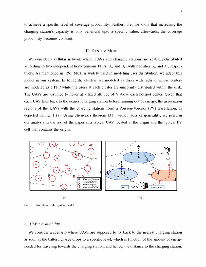
II. SYSTEM MODEL
We consider a cellular network where UAVs and charging stations are spatially-distributed
according to two independent homogeneous PPPs, Φu and Φc, with densities λu and λc, respec-
tively. As mentioned in [26], MCP is widely used in modeling user distribution, we adapt this
model in our system. In MCP, the clusters are modeled as disks with radii rc whose centers
are modeled as a PPP while the users at each cluster are uniformly distributed within the disk.
The UAVs are assumed to hover at a fixed altitude of h above each hotspot center. Given that
each UAV flies back to the nearest charging station before running out of energy, the association
regions of the UAVs with the charging stations form a Poisson-Voronoi (PV) tessellation, as
depicted in Fig. 1 (a). Using Slivnyak’s theorem [31], without loss of generality, we perform
our analysis in the rest of the paper at a typical UAV located at the origin and the typical PV
cell that contains the origin.
Charging StationsAvailable UAVsUser HotspotsCharging UAVs
(a)
Rs,1
Charging StationQueue
hRUo
RU’,n
z
Rs,2
Rcu
Rs,3
(b)
Fig. 1. Illustration of the system model.
A. UAV’s Availability
We consider a scenario where UAVs are supposed to fly back to the nearest charging station
as soon as the battery charge drops to a specific level, which is function of the amount of energy
needed for traveling towards the charging station, and hence, the distance to the charging station.

6
TABLE I
TABLE OF NOTATIONS
Notation Description
Φc, Φc,a; λc, λ′c PPP of charging stations, PPP of active charging stations; density of the charging stations, density of active charging stations
Φu, Φu′ ; λu, λ
′u PPP of UAVs, PPP of available UAVs; density of UAVs, density of available UAVs
Φuo ; Φu′l; Φu
′n
Location of the typical UAV, available LoS UAVs, available NLoS UAVs, respectively
Rs, Rc Horizontal distances between the typical UAV and the typical charging charging station, and the nearest active charging station, respectively
c; N ; Ratio Charging station capacity; the number of UAVs in the typical PV cell; refers to λu/λc
Si, S(i,j); px, Pi Waiting time states, substates; probability that the charging station holds x UAVs, and that it stays in state Si
h; aave UAV altitude; average acceleration while landing/taking off
Vmax, V Maximum velocity while landing or taking off, UAV’s velocity during traveling
Tse, Tse,E Service time, expectation of service time
Tw(i) Waiting time in state i
Ttra, Ttra,E Time required to travel to or from the nearest charging station, expectation of traveling time
Tch, Tland Time used in recharging and landing or taking off, respectively
El, Et Energy consumed in landing or taking off and in traveling, respectively
CRs , CRc Typical charging station which is the nearest to the origin and the nearest active charging station (excluding CRs )
Pa, PC,a, PCrs,a UAV’s availability probability, activity probability of charging stations, and CRs , respectively
Pm, Ps Power consumed during traveling and service, respectively
RUo , RU′,l, RU
′,n Distances between the typical user and the typical UAVs, nearest available LoS UAV, and nearest available NLoS UAV, respectively
Rsu, Rcu Distances between the typical user and CRs and CRc , respectively
ALoS, ANLoS Probability of associating with nearest LoS UAVs and NLoS UAVs, respectively
ACs, ACc Probability of associating with CRs and CRc , respectively
The capacity of each charging stations c is finite, which means they can only charge1 c UAVs
simultaneously. Hence, the UAVs may wait in a queue, and the waiting time Tw depends on the
length of the queue. For the queue analysis, we consider a discrete-time series with the time slot
of length Tch, during which at most c UAVs can be charged simultaneously. To enable analytical
tractability, we assume that the charging process starts at the beginning of each time slot and
the charging UAV leaves at the end of the slot. For a given number of UAVs N in the typical
PV cell, we assume that each of the rest of the UAVs, aside from the typical UAV located at
the origin, have the following probability of being at the typical charging station
Pch(i) =Tch + Tw(i)
Tch + Tw(i) + 2Tland + 2Ttra,E + Tse,E
, (1)
where Tch is the time required for charging, Ttra,E and Tse,E are the average values of the
required time to travel to and from the nearest charging station and the time spent at the hotspot
center to provide service, respectively, and Tland is the time spent during landing or taking off.
Accordingly, Ttra,E, Tse,E, Tland and Tw can be formally defined as follows
Tse,E =Bmax − 2Pm
E[Rs]V− 2El
Ps
, (2)
1In this paper, we use the term ”charging time” to refer to either (i) battery swapping or (ii) battery charging.

7
Ttra,E =E[Rs]
V, (3)
Tland = 2
√2h
aave
, (4)
Tw(i) = i× Tch, (5)
where Bmax is the UAV battery size, Rs is the distance between a UAV and its nearest charging
station, Pm denotes the power consumption during traveling, V is the UAV’s velocity while
traveling, Ps is the power consumption during hovering at the hotspot center, which includes both
the propulsion power and the total communication power, aave is the average acceleration while
landing and taking off, El is the corresponding energy consumption, E[·] denotes expectation
operator, and Tw(i) is the waiting time.
The value of Tw(i) is a function of the state of the queue at the charging station i, which is
explained in the below definition.
Definition 1 (Waiting Time State). We define different states Si and substates S(i,j), in which i
reflects the waiting time Tw(i) = i× Tch, j denotes that there are ci + j UAVs at the charging
station, and j < c holds for all scenarios. Let Pi(t) denote the probability the the charging
stations staying is in state Si at time t, in steady state we have
limt→∞
Pi(t) = Pi.
When the charging station is at the state S(0,j), at most c− j UAVs that arrive during a given
time slot will finish charging before the beginning of the next time slot.
As mentioned, UAVs are available and can provide service to users when they are not traveling
to charging stations or waiting in the queue.
Definition 2 (Availability Probability). We define the event A that indicates the availability of
the typical UAV, which denotes that the UAV is hovering and provides service. Conditioned on
N UAVs in the typical PV cell, the availability probability, which is a fraction of time, of the
UAV is
P(A|N) =∑i
PiEΦc
[Tse(x)
Tse(x) + Tch + Tw(i) + 2Ttra(x) + 2Tland
], (6)
where,
Ttra(x) =Rs(x)
V, (7)
Tse(x) =Bmax − 2Pm
Rs(x)V− 2El
Ps
. (8)

8
Hence, the uncoditioned availability probability is
Pa = EN[P(A|N)], (9)
where x annotates the typical UAV’s location.
In order to enhance the performance of the network and reduce the influence of the frequent
recharging process, we consider a scenario where the UAV can reactivate itself and provide
service as soon as at reaches the charging station. In that case, the charging stations can behave
like a TBS if at least one UAV is recharging.
Definition 3 (Active Charging Station). An active charging station is a charging station that
is occupied by at least one UAV. The point process modeling the locations of active charging
stations is denoted as Φc,a, with density λ′c = λcPC,a, in which
PC,a = 1− PS(0,0),
PS(0,0)=∞∑n=0
P(S(0,0)|N)P(N = n),
where PS(0,0)is the probability the the queuing system staying in state S(0,0). We refer to PC,a
as the activity probability in the rest of the paper.
When the typical UAV is not available, the activity probability of the typical charging station
CRs is different from PC,a and can be computed as follows
PCrs,a = 1− PS(0,0)(1− Pr),
where Pr is the probability that the typical UAV is either charging or waiting at the queue of
the typical charging station, given that the typical UAV is unavailable, which can be computed
as follows
Pr =∑i=0
PiEΦc
[Tw(i) + Tch
2Tland + 2Ttra(x) + Tw(i) + Tch
].
To analyze the coverage probability of this setup, it is important to characterize the distance
distribution between the cluster center and (i) the typical charging station CRs , and (ii) the nearest
active charging station in the point process Φc,a\CRs .
B. Power Consumption
We consider the UAV’s power consumption composed of three parts: (i) service-related power
Ps, including hovering and communication-related power, (ii) traveling power Pm, which denotes
the power consumed in traveling to/from the nearest charging station through the horizontal
9
distance Rs, and (iii) landing and taking off energy El, which owes to the difference in height
between the charging stations and UAV’s altitude.
Based on [10], Pm is a function of the UAV’s velocity V and given by
Pm = P0
(1 +
3V 2
U2tip
)+Piv0
V+
1
2d0ρsAV
3,
where P0 and Pi present the blade profile power and induced power, Utip is the tip speed of
the rotor blade, v0 is the mean rotor induced velocity in hover, ρ is the air density, A is the
rotor disc area, d0 is fuselage drag ratio, and s is rotor solidity. Therefore, the energy consumed
during traveling to or from the charging station is
Et =Rs(x)
VPm
=Rs(x)
V
(P0
(1 +
3V 2
U2tip
)+Piv0
V+
1
2d0ρsAV
3
).
We assume that the optimal value of V that minimizes Et is used. Similarly, the energy consumed
during during landing/taking off is
El =
∫ √2haave
0
Pm(aavet)tdt+
∫ √2haave
0
Pm(Vmax − aavet)tdt,
in which,
Vmax =√
2haave,
where aave denotes the average acceleration while landing or taking off.
C. User Association
Without loss of generality, we focus on a typical user randomly selected from the typical
hotspot centered at the origin. The user associates with the UAV deployed at its hotspot center
if it is available. The set Φuo is composed of only one point, which is the location of the typical
UAV, when it is available, otherwise, Φuo = ∅. If it is unavailable (for charging purposes), the
user associates with the UAV in Φu′ (which presents the locations of all available UAVs) or the
active charging station that provides the largest average received power, as depicted in Fig. 1
(b). The point process Φu′ is constructed by independently thinning Φu with the probability Pa.
Hence, the density of Φu′ is λ′u = Paλu.
When the typical user associates with a UAV, the received power is
pu =
pl = ηlρuGlR−αlu , in case of LoS,
pn = ηnρuGnR−αnu , in case of NLoS,
where ρu is the transmission power of the UAVs, Ru denotes the distance between the typical
user and the serving UAV, αl and αn present the path-loss exponent, Gl and Gn are the fading
10
gains that follow gamma distribution with shape and scale parameters (ml,1ml
) and (mn,1mn
),
ηl and ηn denote the mean additional losses for LoS and NLoS transmissions, respectively. The
probability of establishing an LoS link between the typical user and a UAV at distance Ru is
given in [32] as
Pl(Ru) =1
1 + A exp
(−B
(180π
arctan
(h√
R2u−h2
)− A
)) , (10)
where A and B are two variables that depend on the type of the environment (e.g., urban, dense
urban, and highrise urban), and h is the altitude of the UAV. Consequently, the probability of
NLoS is Pn(Ru) = 1− Pl(Ru).
When the user associates with an active charging station, the received power is
pc = ρuHR−αt
{su,cu},
in which R{su,cu} denotes the distances between the user and CRs and CRc (which are the typical
charging station and the nearest active charging station), respectively, H is the fading gain that
follows exponential distribution with unity mean, and αt presents the path-loss exponent.
The typical user is successfully served if the SINR of the serving link is above a predefined
threshold. We refer to the probability of the SINR greater than this threshold as the coverage
probability.
Definition 4 (Coverage Probability). The total coverage probability is defined as
Pcov = PaPcov,Uo + (1− Pa)Pcov,Uo, (11)
in which,
Pcov,{Uo,Uo} = P(SINR{Uo,Uo} ≥ θ
),
where Pcov,Uo and Pcov,Uoare the coverage probabilities when the typical UAV is available and
unavailable, respectively. Let Φu′l
and Φu′nbe subsets of Φu′ , which denote the locations of LoS
UAVs and NLoS UAVs, respectively. Conditioning on the serving UAV (or active charging station)
located at us, the aggregate interference is defined as
I =∑
Ni∈Φu′n/us
ηnρuGnD−αnNi
+∑
Lj∈Φu′l
/us
ηlρuGlD−αlLj
+∑
Ck∈Φc,a∪{CRs}/us
ρuHD−αtCk
,
in which DNi, DLj
and DCkare the distances between the typical user and the interfering NLoS,
LoS UAVs, and active charging stations, respectively.
III. AVAILABILITY PROBABILITY
To capture the waiting time of the reference UAV in the charging station, we first derive the
probability distribution of the number of UAVs lying in the typical PV cell.

11
The association region of a charging station is the region of the Euclidean plane in which all
UAVs are served by the corresponding charging station. The association cells form the PV cells
generated by Φc. Moreover, the typical UAV is more likely to lie in a larger association cell
than in a smaller one. In other words, the area of the typical PV cell is biased.
Lemma 1 (Number of UAVs Inside a Biased Area). The PMF of the number of UAVs falling
in the typical PV cell is given by
P (N = n) =Γ(a+ n+ 1)
Γ(a)
ba
n!
(λuλc
)n(b+ λu
λc
)a+n+1 , (12)
in which a and b are two fitting parameters for the area of PV cells, and Γ(·) denotes the Gamma
function.
Proof: See Appendix A.
In the rest of the paper, we refer to the ratio λuλc
as Ratio. Having characterized the distribution
of the number of UAVs inside the typical PV cell, we now perform analysis at waiting time
states.
We consider a scenario where the typical cell contains N UAVs, including the typical one.
At the beginning of a new time interval, say tch(1), the system starts at state Si1 and substate
S(i1,j1). If so, there are ci1 +j1 UAVs in that cell and the waiting time is Tw(i1) = i1×Tch. Let m
denotes the number of UAVs that are not in the charging station, which equals to N − ci1 − j1.
If k UAVs come to the charging station during this time slot, then the system transfers to a
new state Si2 and substate S(i2,j2) at the beginning of a the next time slot tch(2). The number of
UAVs arriving to the charging station during (tch(1), tch(2)] is modeled as a Binomial random
variable with an arrival rate Pch(i1).
Lemma 2 (Number of UAVs at charging station). Let pn1(tch(1)) be the probability of the
charging station holds n1 UAVs at time tch(1), in which n1 = ci1 + j1. Consequently, n2 UAVs
present at time tch(2) either arrived during the (tch(1), tch(2)] or were already waiting at time
tch(1). The probability of having n2 UAVs at the charging station at the beginning of a new time
slot tch(2) is
pn2(tch(2)) =
c∑n1=0
pn1(tch(1))
c−n1∑k1=0
(m
k1
)P k1
ch (i1)(1− Pch(i1))m−k1 , n2 = 0,
min(N−c,c+n2)∑n1=0
pn1(tch(1))
(m
k
)P k
ch(i1)(1− Pch(i1))m−k, 0 < n2 < N − c,
12
in which, m = N−ci1−j1, k = n2 +c−n1 and Pch(i) is given in (1). The stationary distribution
of pn2 can be derived as follows
pn2 =
c∑n1=0
pn1
c−n1∑k1=0
(m
k1
)P k1
ch (i1)(1− Pch(i1))m−k1 , n2 = 0,
min(N−c,c+n2)∑n1=0
pn1
(m
k
)P k
ch(i1)(1− Pch(i1))m−k, 0 < n2 < N − c.
Solving the above system of equations, along with∑N
n1=0 pn1 = 1, enables computing the values
of pni .
Proof: The relationships between p(0,n1,...N) can be simply considered as the difference
between new comers and those finished charging during (tch(1), tch(2)]. The corresponding
arrival process is modeled by the binomial distribution B(k, Pch(i)). That is, (tch(1), tch(2)]
is an arbitrary time interval of length Tch, during which k new arrivals will take place with
probability(mk
)P k
ch(i1)(1− Pch(i1))(m−k).
Now we proceed to present the probability of waiting time state.
Lemma 3 (Steady State). The steady state probability Pi is given by
Pi =
c(i+1)−1∑n=ci
pn.
Proof: Observe that pn indicates the probability of n UAVs in the charging station and pci
to pc(i+1)−1 reflect the probability of state Si. Summing pci to pc(i+1)−1 directly completes the
proof.
As stated earlier, Tw(i) has an impact on availability probability and varies from one cell to
the other. Conditioned on a typical PV cell, which contains the typical UAV located at the origin,
we now can derive the conditioned availability probability.
Lemma 4 (Conditioned Availability Probability). For the analysis that follows, let Imax be the
last state that has the longest waiting time, in which Imax = bNcc. Given the value of N , the
availability probability can be written as
P(a|N) =Imax−1∑i=0
Pi
∫ a1a3(i)
a5
1− exp
(− λcπ
(−a1 + a3(i)y
−a2 − a4y
)2)dy, (13)
in which,
a1 = V (Bmax − 2El),
a2 = 2Pm,
13
a3(i) = V
(Bmax − 2El + PsTch(1 + i) + 4Ps
√2h
aave
),
a4 = 2(Ps − Pm),
a5 =2Pma1 − a2V (Bmax − 2El)
2Pma3(i) + a4V (Bmax − 2El).
Proof: See Appendix B
In the following theorem, we derive the availability probability.
Theorem 1 (Availability Probability). The availability probability of the UAV is
Pa =∞∑n=0
P(a|N)P(N = n)
=∞∑n=0
P(a|N)Γ(a+ n+ 1)
Γ(a)
ba
n!
λa+1c λnu
(bλc + λu)a+n+1.
Proof: The above expression follows by substituting (12) and (13) into (9).
IV. COVERAGE PROBABILITY
It can be observed from the previous discussion that after removing the unavailable UAVs form
the original point process Φu, the available UAVs form a new PPP Φu′ with density λ′u = Paλu.
Recalling the association policy in Sec. II-C, the typical user is served by the UAV in its hotspot
center if it is available, otherwise, it associates with the nearest LoS/NLoS UAV or active charging
station, whichever provides the strongest average received power. As stated earlier, the locations
of LoS and NLoS available UAVs are modeled by the PPPs Φu′l, Φu′n
, the location of the typical
UAV is modeled by Φuo (which equals to ∅ when the typical UAV is unavailable), the locations
of the active charging stations (excluding the typical charging station) are modeled by the PPP
Φc,a, and the location of the typical charging station is modeled by CRs.
In order to compute the coverage probability, the distance distribution to the nearest point
in each of these point processes is required, as well as the joint distributions between some of
them, as will be clarified in the following part of the paper.
Lemma 5 (Distance Distribution). The probability density function of the distances between the
typical user and the UAV in its hotspot center, the nearest available NLoS and LoS UAV, denoted
by fRuo(r), fR
u′,n
(r) and fRu′,l(r), respectively, are given by
fRuo(r) =
2r
r2c
, h ≤ r ≤√r2c + h2, (14)
fRu′,n
(r) = 2πλ′
uPn(r)r exp
(− 2πλ
′
u
∫ √r2−h20
zPn(√z2 + h2)dz
), (15)
14
fRu′,l(r) = 2πλ
′
uPl(r)r exp
(− 2πλ
′
u
∫ √r2−h20
zPl(√z2 + h2)dz
), (16)
where Pn(r) and Pl(r) are defined in (10). Recall that Rc and Rs are the distances from the
cluster origin to the nearest active charging station CRc and the typical charging station CRs ,
respectively. Note that Rc is greater than Rs by construction. The PDF of Rc is
fRc(r|Rs) =2πλ
′cr exp(−πλ′cr2)
exp(−πλ′cR2s )
, r ≥ Rs. (17)
Let Rsu and Rcu be the distances between the typical user and CRs and CRc , respectively.
Conditioned on Rs and Rc, their PDFs are given by
fR{su,cu}(r|R{s,c}) =
2r
r2c
, if 0 < r < rc −R{s,c},
2r
πr2c
arccos
(r2 − r2
c +R2{s,c}
2R{s,c}r
), if rc −R{s,c} < r < R{s,c} + rc,
(18)where R{s,c} < rc. Otherwise,
fR{su,cu}(r|R{s,c}) =2r
πr2c
arccos
(r2 − r2
c +R2{s,c}
2R{s,c}r
), if R{s,c} − rc < r < R{s,c} + rc.
(19)Hence, the CDFs of Rsu and Rcu are given by
FR{su,cu}(r|R{s,c}) =
r2
r2c, if 0 < r < rc −R{s,c},
∫ rrc−R{s,c}
2x arccos
(x2−r2c+R
2{s,c}
2R{s,c}x
)dx
πr2c+
(rc −R{s,c})2
r2c, if rc −R{s,c} < r < R{s,c} + rc,
1, if R{s,c} + rc < r,
(20)when R{s,c} < rc. Otherwise,
FR{su,cu}(r|R{s,c}) =
∫ rR{s,c}−rc
2x arccos
(x2−r2c+R2
{s,c}2R{s,c}x
)dx
πr2c
, if R{s,c} − rc < r < R{s,c} + rc,
1, if R{s,c} + rc < r.
(21)
Now that we have derived all the required distance distributions, in the following part, we
aim to characterize the association probability with each of the UAVs and the active charging
stations when the the typical UAV is unavailable.
Lemma 6 (Associate Probability). Let ALoS(r), ANLoS(r), ACs(r) and ACc(r) be the probabil-
ities that the typical user associates with the nearest LoS, NLoS UAV, CRs and CRc at distance
r, respectively. When CRs is active, the association probabilities are given by
ALoS,a(r|Rs, Rc) = ALoS−NLoS(r)ALoS−Cs(r|Rs)ALoS−Cc(r|Rc),
15
ANLoS,a(r|Rs, Rc) = ANLoS−LoS(r)ANLoS−Cs(r|Rs)ANLoS−Cc(r|Rc),
ACs(r|Rs, Rc) = ACs−LoS(r|Rs)ACs−NLoS(r|Rs)ACs−Cc(r|Rs, Rc),
ACc,a(r|Rs, Rc) = ACc−LoS(r|Rc)ACc−NLoS(r|Rc)ACc−Cs(r|Rs, Rc).
When CRs is not active, the association probabilities are given by
ALoS,n(r|Rc) = ALoS−NLoS(r)ALoS−Cc(r|Rc),
ANLoS,n(r|Rc) = ANLoS−LoS(r)ANLoS−Cc(r|Rc),
ACc,n(r|Rc) = ACc−LoS(r|Rc)ACc−NLoS(r|Rc),
in which,
ALoS−NLoS(r) = exp
(− 2πλ
′
u
∫ √d2n(r)−h2
0
zPn(√z2 + h2)dz
),
ANLoS−LoS(r) = exp
(− 2πλ
′
u
∫ √d2l (r)−h2
0
zPl(√z2 + h2)dz
),
A{LoS,NLoS}−{Cs,Cc}(r|R{s,c}) = 1− FR{su,cu}(D{l,n}(r|R{s,c})),
A{Cs,Cc}−{Cc,Cs}(r|R{c,s}) = 1− FR{cu,su}(r|R{c,s}),
A{Cs,Cc}−{LoS,NLoS}(r|R{s,c}) = exp
(− 2πλ
′
u
∫ √D2{l,n}(r)−h2
0
zP{l,n}(√z2 + h2)dz
),
where D{l,n}(r) = rα{l,n}αt η
1αt
{l,n}, Dl(r) = max
(h, r
αtαl η
1αll
), Dn(r) = max
(h, r
αtαn η
1αnn
),
dl(r) =
(ηl
ηn
) 1αl
rαnαl , (22)
and
dn(r) = max
(h,
(ηn
ηl
) 1αn
rαlαn
). (23)
Proof: See Appendix C.
The final requirement to derive the coverage probability is the Laplace transform of the
aggregate interference, which is provided in the following lemma.
Lemma 7 (Laplace Transform of Interference). Using subscripts a and n to capture the events
of the typical charging station is active and inactive, respectively, the Laplace transform of the
interference power conditioned on the serving UAV us located at x is
LI,{a,n}(s, ‖x‖) = exp
(−2πλ
′
u
∫ ∞a(‖x‖)
[1−
(mn
mn + sηnρu(z2 + h2)−αn2
)mn]zPn(√z2 + h2)dz
)× exp
(−2πλ
′
u
∫ ∞b(‖x‖)
[1−
(ml
ml + sηlρu(z2 + h2)−αl2
)ml]zPl(√z2 + h2)dz
)

16
× exp
(−2πλ
′
c
∫ ∞c(‖x‖)
[1−
(1
1 + sρuz−αt
)]zdz
),
in which,
a(‖x‖) =
0, if us ∈ Φuo ,√d2
n(‖x‖)− h2, if us ∈ Φu′l,√
‖x‖2 − h2, if us ∈ Φu′n,√
D2n(‖x‖)− h2, if us ∈ Φc,a ∪ {CRs},
b(‖x‖) =
0, if us ∈ Φuo ,√‖x‖2 − h2, if us ∈ Φu
′l,√
d2l (‖x‖)− h2, if us ∈ Φu′n
,√D2l (‖x‖)− h2, if us ∈ Φc,a ∪ {CRs},
c(‖x‖) =
0, if us ∈ Φuo ,
Dl(‖x‖), if us ∈ Φu′l,
Dn(‖x‖), if us ∈ Φu′n,
Rcu, if us ∈ Φc,a ∪ {CRs} and CRs is inactive,
min(Rsu, Rcu), if us ∈ Φc,a ∪ {CRs} and CRs is active,Proof: See Appendix D.
Now that we have developed expressions for the relevant distances and the association prob-
abilities, we study the coverage probability as explained in Definition 4.
Theorem 2 (Coverage Probability). The coverage probability, provided in (11), can be computed
using the following expressions for the coverage probability when the typical UAV is available
and unavailable, respectively:
Pcov,Uo = Pcov,Uo,l+ Pcov,Uo,n ,
Pcov,Uo= Pcov,U
′l+ Pcov,U′n
+ Pcov,Cs + Pcov,Cc,
where,
Pcov,Uo,l=E{Rs,Rc,Rcu,Rsu}
[ ∫ √h2+r2c
h
ml−1∑k=0
(−mlgl(r))k
k!
×[PC,a
∂k
∂skLσ2+I,a(s, r) + (1− PC,a)
∂k
∂skLσ2+I,n(s, r)
]s=mlgl(r)
Pl(r)2r
r2c
dr
], (24)
17
Pcov,Uo,n =E{Rs,Rc,Rcu,Rsu}
[ ∫ √h2+r2c
h
mn−1∑k=0
(−mngn(r))k
k!
×[PC,a
∂k
∂skLσ2+I,a(s, r) + (1− PC,a)
∂k
∂skLσ2+I,n(s, r)
]s=mngn(r)
Pn(r)2r
r2c
dr
], (25)
Pcov,U′l
=E{Rs,Rc,Rcu,Rsu}
[ ∫ ∞h
ml−1∑k=0
(−mlgl(r))k
k!
(ALoS,a(r|Rs, Rc)PCrs,a
∂k
∂skLσ2+I,a(s, r)
+ALoS,n(r|Rc)(1− PCrs,a)∂k
∂skLσ2+I,n(s, r)
)s=mlgl(r)
fRu′,l(r)dr
], (26)
Pcov,U′n=E{Rs,Rc,Rcu,Rsu}
[ ∫ ∞h
mn−1∑k=0
(−mngn(r))k
k!
(ANLoS,a(r|Rs, Rc)PCrs,a
∂k
∂skLσ2+I,a(s, r)
+ANLoS,n(r|Rc)(1− PCrs,a)∂k
∂skLσ2+I,n(s, r)
)s=mngn(r)
fRu′,n
(r)dr
], (27)
Pcov,Cs =E{Rs,Rc,Rcu}
[ ∫ ∞0
(ACs(r|Rs, Rc)PCrs,aLσ2+I,a(θρ−1
u rαT , r)
)fRsu(r|Rs)dr
], (28)
Pcov,Cc =E{Rs,Rc,Rsu}
[ ∫ ∞0
(ACc,a(r|Rs, Rc)PCrs,aLσ2+I,a(θρ−1
u rαT , r)
+ACc,n(r|Rc)(1− PCrs,a)Lσ2+I,n(θρ−1u rαT , r)
)fRcu(r|Rc)dr
], (29)
in which
gl(r) = θη−1l ρ−1
u rαl ,
gn(r) = θη−1n ρ−1
u rαn , (30)
fRc(r|Rs) is given in (17), and fRs(r) = 2λcπr exp(−λcπr2).
Proof: See Appendix E.
Note that the summations and derivatives in Theorem 2 are obtained fromΓu(m,mg)
Γ(m)= exp(−mg)
m−1∑k=0
(mg)k
k!,
and
EU [exp(−sU)Uk] = (−1)k∂k
∂skLU(s).
Observe that the above expressions require evaluating higher order derivatives of the Laplace
transform. Now we present an approximation for the coverage probability using the upper bound
of the CDF of the Gamma distribution [33].

18
Lemma 8 (Approximated Coverage Probability). Pcov,Uo,{l,n} and Pcov,U′{l,n}
can be approximated
by using the upper bound of the CDF of the Gamma distribution as
Pcov,Uo,{l,n} = E{Rs,Rc,Rcu,Rsu}
[m{l,n}∑k=1
(m{l,n}k
)(−1)k+1
∫ √h2+r2c
h
P{l,n}(r)2r
r2c
×(PC,aLσ2+I,a(kβ2m{l,n}g{l,n}(r), r) + (1− PC,a)Lσ2+I,n(kβ2m{l,n}g{l,n}(r), r)
)dr
], (31)
Pcov,U′{l,n}
= E{Rs,Rc,Rcu,Rsu}
[m{l,n}∑k=1
(m{l,n}k
)(−1)k+1
∫ ∞h
fRu′,{l,n}
(r)
(A{L,NL}oS,a(r|Rs, Rc)×
PCrs,aLσ2+I,a(kβ2mlg{l,n}(r), r) +A{L,NL}oS,n(r|Rc)(1− PCrs,a)Lσ2+I,n(kβ2mlg{l,n}(r), r)
)dr
],
(32)
in which β2 = (m{l,n}!)− 1m{l,n} .
Proof: See Appendix F.
Remark 1. The results in Lemma 8 efficiently reduce the complexity of computing the coverage
probability, since it only requires a simple integral and finite summations. In addition, note that
the fading gain of NLoS is 1 in our system model, we only need to evaluate the integral and no
summations. Besides, it is a tight approximation, whose gap can be ignored, more details will
be shown in Section V.
V. NUMERICAL RESULT
In this section, we validate our analytical results with simulations and evaluate the impact of
various system parameters on the network performance such as the Ratio = λuλc
and the charging
station capacity c. Unless stated otherwise, we use the simulation parameters as listed herein
Table II.
In Fig. 2 we plot the availability probability conditioned on the number of UAVs in the
typical PV cell against the charging station capacity c. For a given value of N , the availability
probability increases with the charging station capacity until the maximum achievable value in
which waiting time equals to 0 min.
The results in Fig. 3 reveal that charging station capacity has a significant impact on the
availability of UAVs. When the capacity is low, the availability probability of UAVs decreases
dramatically with the increase in the Ratio = λuλc
. We also notice that at high values of theλuλc
, say 20, a slight increases in the capacity, from 1 to 2, leads to doubling the availability
probability from 0.2 to 0.4.
19
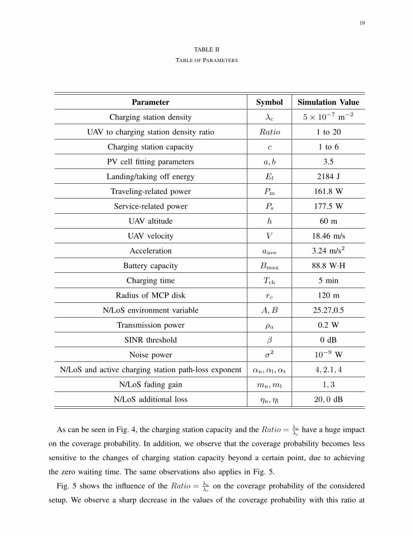
TABLE II
TABLE OF PARAMETERS
Parameter Symbol Simulation Value
Charging station density λc 5× 10⁻⁷ m−2
UAV to charging station density ratio Ratio 1 to 20
Charging station capacity c 1 to 6
PV cell fitting parameters a, b 3.5
Landing/taking off energy El 2184 J
Traveling-related power Pm 161.8 W
Service-related power Ps 177.5 W
UAV altitude h 60 m
UAV velocity V 18.46 m/s
Acceleration aave 3.24 m/s2
Battery capacity Bmax 88.8 W·H
Charging time Tch 5 min
Radius of MCP disk rc 120 m
N/LoS environment variable A,B 25.27,0.5
Transmission power ρu 0.2 W
SINR threshold β 0 dB
Noise power σ2 10−9 W
N/LoS and active charging station path-loss exponent αn, αl, αt 4, 2.1, 4
N/LoS fading gain mn,ml 1, 3
N/LoS additional loss ηn, ηl 20, 0 dB
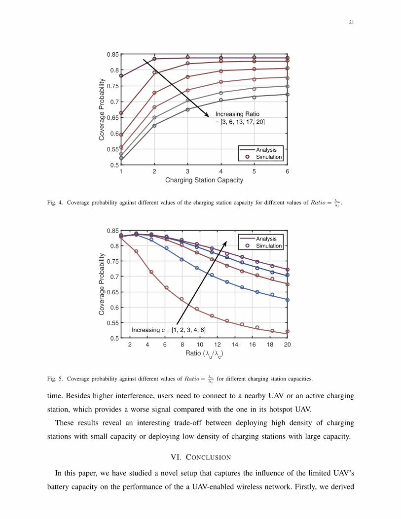
As can be seen in Fig. 4, the charging station capacity and the Ratio = λuλc
have a huge impact
on the coverage probability. In addition, we observe that the coverage probability becomes less
sensitive to the changes of charging station capacity beyond a certain point, due to achieving
the zero waiting time. The same observations also applies in Fig. 5.
Fig. 5 shows the influence of the Ratio = λuλc
on the coverage probability of the considered
setup. We observe a sharp decrease in the values of the coverage probability with this ratio at

20
1 2 3 4 5 6
Charging Station Capacity
0.1
0.2
0.3
0.4
0.5
0.6
0.7
0.8
P(a
|N)
Analysis
Simulation
Increasing N = [7, 14, 19, 25]
Fig. 2. Conditioned availability probability of UAVs for different values of the charging station capacity for different values of
N . Dash line denotes the maximum achievable availability probability in which there is no waiting time at the charging station.
2 4 6 8 10 12 14 16 18 20
Ratio (u/
c)
0.2
0.3
0.4
0.5
0.6
0.7
0.8
0.9
Availa
bili
ty P
robabili
ty
Analysis
Simulation
Increasing Capacity
= [1, 2, 3, 4, 5, 6]
Fig. 3. Probability of availability against different values of the Ratio = λuλc
for different charging station capacities.
smaller values of the charging station capacity. For instance, at c = 1, the coverage probability
drops from 0.83 to 0.52 as we increase the ratio from 1 to 20, which is consistent with sharp
decrease in availability probability. However, the influence becomes much less as we increase the
charging station capacity. Coverage probability increases first due to the fact that the typical user
is more likely to establish a LoS link with serving UAV. However, if we continue increasing the
density of UAVs, availability probability decreases quickly owing to a long queue and waiting
21
1 2 3 4 5 6
Charging Station Capacity
0.5
0.55
0.6
0.65
0.7
0.75
0.8
0.85
Covera
ge P
robabili
ty
Analysis
Simulation
Increasing Ratio
= [3, 6, 13, 17, 20]
Fig. 4. Coverage probability against different values of the charging station capacity for different values of Ratio = λuλc
.
2 4 6 8 10 12 14 16 18 20
Ratio (u/
c)
0.5
0.55
0.6
0.65
0.7
0.75
0.8
0.85
Covera
ge P
robabili
ty
Analysis
Simulation
Increasing c = [1, 2, 3, 4, 6]
Fig. 5. Coverage probability against different values of Ratio = λuλc
for different charging station capacities.
time. Besides higher interference, users need to connect to a nearby UAV or an active charging
station, which provides a worse signal compared with the one in its hotspot UAV.
These results reveal an interesting trade-off between deploying high density of charging
stations with small capacity or deploying low density of charging stations with large capacity.
VI. CONCLUSION
In this paper, we have studied a novel setup that captures the influence of the limited UAV’s
battery capacity on the performance of the a UAV-enabled wireless network. Firstly, we derived
22
the availability probability of a UAV as a function of the battery size, the charging time, the
density of UAVs, the density of the charging stations, and the charging station’s capacity. Next,
we used the availability probability to compute the overall coverage probability of the considered
setup. We have shown how the performance of the considered setup degrades as the capacity of
the charging stations decreases or as the ratio between the density of the UAVs and the density
of the charging stations increases.
This work tapped a new aspect of the performance of UAV-enabled wireless networks, which
can be expanded in various directions. For instance, the performance could be enhanced if each
charging station schedules the arrivals and departures of the UAVs to avoid conflicts. The optimal
scheduling given the locations of the locations of the UAVs, the charging time, and the power
consumption model, is a very interesting open problem.
APPENDIX
A. Proof of Lemma 1
We adopt the two-parameter gamma function in [34] to fit the area of PV cells
f(y) =ba
Γ(a)y(a−1)e−by, (33)
in which, a and b are two fitting parameters. As for a typical UAV, the probability that it locates
in the typcial PV cell is proportional to the area of that cell [35]. The PDF of the biased area
A′c is given by
fA′c(c) =
cfAc(c)
E[Ac]=
ba
Γ(a)λc(cλc)
ae−bcλc , (34)
in which fAc(c) = ba
Γ(a)λc(cλc)
(a−1)e−bcλc is the PDF of the unbiased area.
The number of UAVs per PV cell is a Poisson distributed random variable, that is
P(N = n) = EA′c[P(N = n|A′c)] =
∫ ∞0
P(N = n)fA′c(c)dc
=
∫ ∞0
(λuc)ne−λuc
n!
ba
Γ(a)λc(cλc)
ae−bcλcdc =Γ(a+ n+ 1)
Γ(a)
ba
n!
λa+1c λnu
(bλc + λu)a+n+1. (35)
B. Proof of Lemma 4
Let
P(a|N,S) = EΦc
[Tse
Tse + Tch + Tw(i) + 2Ttra(x) + 2Tland
], (36)
P(a|N,S,Rs) =Tse
Tse + Tch + Tw(i) + 2Ttra(x) + 2Tland
, (37)
23
we refer to event S as conditioned state of waiting time. Substituting (4), (5), (7) and (8) into
(37), that is
P(a|N,S,Rs) =V (Bmax − 2El)− 2PmRs(x)
V
(Bmax − 2El + PsTch(1 + i) + 4Ps
√2ha
)+ 2Rs(x)(Ps − Pm)
=a1 − a2Rs(x)
a3(i) + a4Rs(x), (38)
in which a1, a2, a3(i) and a4 has been defined in Lemma 4.
The CDF of P(a|N,S,Rs) is defined as
FP(a|N,S,Rs)(y) = P
(a1 − a2Rs(x)
a3(i) + a4Rs(x)≤ y
), (39)
given that P(a|N,S,Rs) is a decreasing function of Rs, the preimage can be obtained as follows
FP(a|N,S,Rs)(y) = P
(Rs(x) ≥ −a1 + a3(i)y
−a2 − a4y
)(a)=
∫ ∞−a1+a3(i)y−a2−a4y
2λcπre−λcπr2dr = exp
(− λcπ
(−a1 + a3(i)y
−a2 − a4y
)2), (40)
step (a) follows from the fact that Rs(x) is the first contact distance of PPP. Note that due to
assuming the typical UAV to be at the origin, Rs(x) = ‖x‖. Substituting (40) into (36)
P(a|N,S) = EΦc [P(a|N,S,Rs)] =
∫ ∞0
1− FP(a|N,S,Rs)(y)dy =
∫ a1a3(i)
a5
1− exp
(− λcπ
(−a1 + a3(i)y
−a2 − a4y
)2)dy.
(41)Substituting (41) and 0 ≤ i ≤ Imax − 1 into (6) completes the proof.
C. Proof of Lemma 6
When the typical UAV is unavailable, the typical user associates receives more power from
the nearest LoS UAV than the nearest NLos UAV with the following probability:
ALoS−NLoS(r) = P(ηlρur
−αl > ηnρuR−αn
u′ ,n
)= P
(RU′ ,n > (
ηn
ηl
)1αn r
αlαn
)= P
(RU′ ,n > (
ηn
ηl
)1αn r
αlαn
)= exp
(− 2πλ
′
u
∫ √d2n(r)−h2
0
zPn(√z2 + h2)dz
),
(42)in which dn(r) is given in Lemma 6. The proofs of other association probabilities are similar to
ALoS−NLoS(r), therefore omitted here.
D. Proof of Lemma 7
The aggregate interference power and its corresponding Laplace transform is conditioned on
the serving UAV us located at x, given by
LI,{a,n}(s, ‖x‖) = EI[exp(−sI)]
24
=EΦu′n
[ ∏Ni∈Φ
u′n/us
exp(−sηnρuGnD−αnNi
)
]× EΦ
u′l
[ ∏Lj∈Φ
u′l
/us
exp(−sηlρuGlD−αlLj
)
]
× EΦc,a
[ ∏Ck∈Φc,a∪CRs/us
exp(−sρuHD−αtCk
)
]
=EΦu′n
[ ∏Ni∈Φ
u′n/us
Egn [exp(−sηnρuGnD−αnNi
)]
]× EΦ
u′l
[ ∏Lj∈Φ
u′l
/us
Egl [exp(−sηlρuGlD−αlLj
)]
]
× EΦc,a
[ ∏Ck∈Φc,a∪CRs∪CRs/us
EH[exp(−sρuHD−αtCk
)]
](a)=EΦ
u′n
[ ∏Ni∈Φ
u′n/us
(mn
mn + sηnρuD−αnNi
)mn]× EΦ
u′l
[ ∏Lj∈Φ
u′l
/us
(ml
ml + sηlρuD−αlLj
)ml]
× EΦc,a
[ ∏Ck∈Φc,a∪CRs/us
(1
1 + sρuD−αlCk
)](b)= exp
(−2πλ
′
u
∫ ∞a(‖x‖)
[1−
(mn
mn + sηnρu(z2 + h2)−αn2
)mn]zPn(√z2 + h2)dz
)× exp
(−2πλ
′
u
∫ ∞b(‖x‖)
[1−
(ml
ml + sηlρu(z2 + h2)−αl2
)ml]zPl(√z2 + h2)dz
)× exp
(−2πλ
′
c
∫ ∞c(‖x‖)
[1−
(1
1 + sρuz−αt
)]zdz
), (43)
where step (a) follows from the moment generating function (MGF) of Gamma distribution,
(b) follows from the PGFL of inhomogeneous PPP, a(‖x‖), b(‖x‖) and c(‖x‖) are defined in
Lemma 7.
E. Proof of Theorem 2
When the typical user is associated with the LoS UAV in its hotspot center, the coverageprobability is given by
Pcov,Uo,l= ERuo
[P(ηlρuGlR
−αluo
σ2 + I≥ θ|Ruo
)Pl(Ruo
)
]= ERuo
[P(Gl ≥
θRαluo
(σ2 + I)
ηlρu|Ruo
)Pl(Ruo
)
](a)= ERuo
[Eσ2+I
[Γu(ml,mlgl(Ruo)(σ2 + I))
Γ(ml)
]Pl(Ruo
)
](b)= ERuo
[Eσ2+I
[e−mlgl(Ruo )(σ
2+I)ml−1∑k=0
(mlgl(Ruo)(σ2 + I))k
k!
]Pl(Ruo
)
]
= ERuo
[Pl(Ruo
)
ml−1∑k=0
(mlgl(Ruo))k
k!Eσ2+I
[e−mlgl(Ruo )(σ
2+I)(σ2 + I)k]]
(c)= ERuo
[ml−1∑k=0
(−mlgl(Ruo))k
k!
[PC,a
∂k
∂skLσ2+I,a(s,Ruo
) + (1− PC,a)∂k
∂skLσ2+I,n(s,Ruo
)
]s=mlgl(Ruo )
Pl(Ruo)
](d)=
∫ √h2+r2c
h
ml−1∑k=0
(−mlgl(r))k
k!
∂k
∂sk
[PC,aLσ2+I,a(s, r) + (1− PC,a)Lσ2+I,n(s, r)
]s=mlgl(r)
Pl(r)2r
r2cdr, (44)
25
where gl(r) and gn(r) are defined in (30), step (a) is due to the definition of CCDF of Gamma
function FG(g) = Γu(m,mg)Γ(m)
, with Γu(m,mg) is the upper incomplete Gamma function [9], step
(b) follows from Γu(m,mg)Γ(m)
= exp(−mg)∑m−1
k=0(mg)k
k!, step (c) is obtained by EU [exp(−sU)Uk] =
(−1)k ∂k
∂skLU(s), and step (d) follows the distribution of Ruo defined in (14).
Conditioned on Rs and Rc, and given that the typical UAV is unavailable, the coverage
probability when associating with the nearest LoS UAV Pcov,U′l
can be written as
Pcov,U′l
= ERU′,l
[ALoS,a(Ru′ ,l|Rs, Rc)PCrs,aP
(ηlρuGlR−αl
u′ ,l
σ2 + I≥ θ|Ru′ ,l
)]+ ER
u′,l
[ALoS,n(Ru′ ,l|Rs, Rc)(1− PCrs,a)P
(ηlρuGlR−αl
u′ ,l
σ2 + I≥ θ|Ru′ ,l
)]= ER
u′,l
[ALoS,a(Ru′ ,l|Rs, Rc)PCrs,a
ml−1∑k=0
(−mlgl(Ru′ ,l))k
k!
∂k
∂skLσ2+I,a(s, Ru′ ,l)|s=mlgl(Ru
′,l
)
]
+ ERu′,l
[ALoS,n(Ru′ ,l|Rs, Rc)(1− PCrs,a)
ml−1∑k=0
(−mlgl(Ru′ ,l))k
k!
∂k
∂skLσ2+I,n(s, Ru′ ,l)|s=mlgl(Ru
′,l
)
]
=
∫ ∞h
[ALoS,a(r|Rs, Rc)(1− PCrs,a)
ml−1∑k=0
(−mlgl(r))k
k!
∂k
∂skLσ2+I,n(s, r)|s=mlgl(r)
+ALoS(r|Rs, Rc)PCrs,a
ml−1∑k=0
(−mlgl(r))k
k!
∂k
∂skLσ2+I,a(s, r)|s=mlgl(r)
]fR
u′,l(r)dr. (45)
where fRu′,l(r) is given in (16). Taking the expectation over Rs and Rc completes the proof.
Pcov,U′n, Pcov,Cs and Pcov,Cc follow a similar method, therefore omitted here.
F. Proof of Lemma 8
Given that (44) and (45) require higher-order derivatives of Laplace transform, we here use
the upper bound of the CDF of the Gamma distribution in order to compute a less complicated
approximation. It has been shown in both [9] and [36] that this upper bound provides a tight
approximation to coverage probability, which can be derived as follows
Eσ2+I
[Γu(m{l,n},mlg{l,n}(r)(σ
2 + I))
Γ(m{l,n})
]= Eσ2+I
[1−
Γl(m{l,n},m{l,n}g{l,n}(r)(σ2 + I))
Γ(m{l,n})
]=1− Eσ2+I
[Γl(m{l,n},m{l,n}g{l,n}(r)(σ
2 + I))
Γ(m{l,n})
](a)≈1− Eσ2+I
[(1− e−β2(m{l,n})m{l,n}g{l,n}(r)(σ
2+I)
)m{l,n}](b)=1− Eσ2+I
[m{l,n}∑k=0
(m{l,n}k
)(−1)ke−kβ2(m{l,n})m{l,n}g{l,n}(r)(σ
2+I)
]

26
=
m{l,n}∑k=1
(m{l,n}k
)(−1)k+1Eσ2+I
[e−kβ2(m{l,n})m{l,n}g{l,n}(r)(σ
2+I)
]
=
ml∑k=1
(m{l,n}k
)(−1)k+1Lσ2+I(kβ2(m{l,n})m{l,n}g{l,n}(r), r), (46)
in which Γl(m,mg) denotes the lower incomplete Gamma function [9] and step (a) follows the
upper bound in
(1− e−β1(m)mg)m <Γl(m,mg)
Γ(m)< (1− e−β2(m)mg)m, (47)
in which,
β1(m) =
1, if m > 1,
(m!)−1m , if m < 1,
β2(m) =
(m!)−1m , if m > 1,
1, if m < 1.(48)
Step (b) results from applying Binomial theorem.
In the case of above approximation, Pcov,Uo,lin (44) and Pcov,U
′l
in (45) can be rewritten as
Pcov,Uo,{l,n} =ERuo
[Eσ2+I
[Γu(m{l,n},m{l,n}g{l,n}(Ruo)(σ
2 + I))
Γ(m{l,n})
]P{l,n}(Ruo)
]
=ERuo
[m{l,n}∑k=1
(m{l,n}k
)(−1)k+1
(PC,aLσ2+I,a(kβ2(m{l,n})m{l,n}g{l,n}(Ruo), Ruo)
+ (1− PC,a)Lσ2+I,n(kβ2(m{l,n})m{l,n}g{l,n}(Ruo), Ruo)
)P{l,n}(Ruo)
]=
m{l,n}∑k=1
(m{l,n}k
)(−1)k+1ERuo
[(PC,aLσ2+I,a(kβ2(m{l,n})m{l,n}g{l,n}(Ruo), Ruo)
+ (1− PC,a)Lσ2+I,n(kβ2(m{l,n})m{l,n}g{l,n}(Ruo), Ruo)
)P{l,n}(Ruo)
]=
m{l,n}∑k=1
(m{l,n}k
)(−1)k+1
∫ √h2+r2c
h
(PC,aLσ2+I,a(kβ2(m{l,n})m{l,n}g{l,n}(r), r)
+ (1− PC,a)Lσ2+I,n(kβ2(m{l,n})m{l,n}g{l,n}(r), r)
)P{l,n}(r)
2r
r2c
dr, (49)
Pcov,U′{l,n}
=ERu′,{l,n}
[A(m{L,NL})oS(Ru′ ,{l,n})P
(η{l,n}ρuG{l,n}R−α{l,n}u′ ,{l,n}
σ2 + I≥ θ|Ru′ ,{l,n}
)]=ER
u′,{l,n}
[ALoS(Ru′ ,{l,n})Eσ2+I
[Γu(m{l,n},m{l,n}g{l,n}(Ru′ ,{l,n})(σ
2 + I))
Γ(m{l,n})
]]
=
m{l,n}∑k=1
(m{l,n}k
)(−1)k+1ER
u′,{l,n}
[A{L,NL}oS(Ru′ ,{l,n})×(
PCrs,aLσ2+I,a(kβ2(m{l,n})m{l,n}g{l,n}(Ru′ ,{l,n}), Ru′ ,{l,n})
+ (1− PCrs,a)Lσ2+I,n(kβ2(m{l,n})m{l,n}g{l,n}(Ru′ ,{l,n}), Ru′ ,{l,n})
)]
27
=
m{l,n}∑k=1
(m{l,n}k
)(−1)k+1
∫ ∞h
A{L,NL}oS(r)fRu′,{l,n}
(r)×(PCrs,aLσ2+I,a(kβ2(m{l,n})m{l,n}g{l,n}(r), r)
+ (1− PCrs,a)Lσ2+I,n(kβ2(m{l,n})m{l,n}g{l,n}(r), r)
)dr. (50)
REFERENCES
[1] S. Sekander, H. Tabassum, and E. Hossain, “Multi-tier drone architecture for 5G/B5G cellular networks: Challenges, trends,
and prospects,” IEEE Communications Magazine, vol. 56, no. 3, pp. 96–103, 2018.
[2] M. Mozaffari, W. Saad, M. Bennis, Y.-H. Nam, and M. Debbah, “A tutorial on UAVs for wireless networks: Applications,
challenges, and open problems,” IEEE Communications Surveys & Tutorials, vol. 21, no. 3, pp. 2334–2360, 2019.
[3] B. Li, Z. Fei, and Y. Zhang, “UAV communications for 5G and beyond: Recent advances and future trends,” IEEE Internet
of Things Journal, vol. 6, no. 2, pp. 2241–2263, April 2019.
[4] Y. Zeng, R. Zhang, and T. J. Lim, “Wireless communications with unmanned aerial vehicles: Opportunities and challenges,”
IEEE Communications Magazine, vol. 54, no. 5, pp. 36–42, May 2016.
[5] N. Cheng, F. Lyu, W. Quan, C. Zhou, H. He, W. Shi, and X. Shen, “Space/aerial-assisted computing offloading for
iot applications: A learning-based approach,” IEEE Journal on Selected Areas in Communications, vol. 37, no. 5, pp.
1117–1129, 2019.
[6] H. Liao, Z. Zhou, W. Kong, Y. Chen, X. Wang, Z. Wang, and S. A. Otaibi, “Learning-based intent-aware task offloading
for air-ground integrated vehicular edge computing,” IEEE Transactions on Intelligent Transportation Systems, pp. 1–13,
2020.
[7] M. Kishk, A. Bader, and M.-S. Alouini, “Aerial base station deployment in 6G cellular networks using tethered drones:
The mobility and endurance tradeoff,” IEEE Vehicular Technology Magazine, vol. 15, no. 4, pp. 103–111, Dec. 2020.
[8] A. Fotouhi, H. Qiang, M. Ding, M. Hassan, L. G. Giordano, A. Garcia-Rodriguez, and J. Yuan, “Survey on UAV
cellular communications: Practical aspects, standardization advancements, regulation, and security challenges,” IEEE
Communications Surveys Tutorials, vol. 21, no. 4, pp. 3417–3442, 2019.
[9] M. Alzenad and H. Yanikomeroglu, “Coverage and rate analysis for vertical heterogeneous networks (VHetNets),” IEEE
Transactions on Wireless Communications, vol. 18, no. 12, pp. 5643–5657, Dec. 2019.
[10] Y. Zeng, J. Xu, and R. Zhang, “Energy minimization for wireless communication with rotary-wing UAV,” IEEE Transactions
on Wireless Communications, vol. 18, no. 4, pp. 2329–2345, April 2019.
[11] L. Yang, J. Chen, M. O. Hasna, and H. Yang, “Outage performance of UAV-assisted relaying systems with RF energy
harvesting,” IEEE Communications Letters, vol. 22, no. 12, pp. 2471–2474, 2018.
[12] Y. Dong, J. Cheng, M. J. Hossain, and V. C. M. Leung, “Extracting the most weighted throughput in UAV empowered
wireless systems with nonlinear energy harvester,” in 2018 29th Biennial Symposium on Communications (BSC), 2018,
pp. 1–5.
[13] S. Sekander, H. Tabassum, and E. Hossain, “Statistical performance modeling of solar and wind-powered UAV
communications,” IEEE Transactions on Mobile Computing, 2020, IEEE Network, to appear.
[14] P.-V. Mekikis and A. Antonopoulos, “Breaking the boundaries of aerial networks with charging stations,” in ICC 2019-2019
IEEE International Conference on Communications (ICC). IEEE, 2019, pp. 1–6.
[15] Z. Zhou, J. Feng, B. Gu, B. Ai, S. Mumtaz, J. Rodriguez, and M. Guizani, “When mobile crowd sensing meets uav: Energy-
efficient task assignment and route planning,” IEEE Transactions on Communications, vol. 66, no. 11, pp. 5526–5538,
2018.
28
[16] B. Galkin, J. Kibilda, and L. A. DaSilva, “UAVs as mobile infrastructure: Addressing battery lifetime,” IEEE Communi-
cations Magazine, vol. 57, no. 6, pp. 132–137, 2019.
[17] Y. Qin, M. A. Kishk, and M.-S. Alouini, “Performance evaluation of UAV-enabled cellular networks with battery-limited
drones,” IEEE Communications Letters, to appear.
[18] M. A. Kishk, A. Bader, and M.-S. Alouini, “On the 3-D placement of airborne base stations using tethered UAVs,” IEEE
Transactions on Communications, vol. 68, no. 8, pp. 5202–5215, Aug. 2020.
[19] O. M. Bushnaq, M. A. Kishk, A. Celik, M.-S. Alouini, and T. Y. Al-Naffouri, “Optimal deployment of tethered drones
for maximum cellular coverage in user clusters,” Transactions on Wireless Communications, to appear.
[20] M. Lahmeri, M. A. Kishk, and M.-S. Alouini, “Stochastic geometry-based analysis of airborne base stations with laser-
powered UAVs,” IEEE Communications Letters, vol. 24, no. 1, pp. 173–177, Jan. 2020.
[21] J. Ouyang, Y. Che, J. Xu, and K. Wu, “Throughput maximization for laser-powered UAV wireless communication systems,”
in IEEE ICC Workshops, 2018.
[22] P. D. Diamantoulakis, K. N. Pappi, Z. Ma, X. Lei, P. C. Sofotasios, and G. K. Karagiannidis, “Airborne radio access
networks with simultaneous lightwave information and power transfer (SLIPT),” in IEEE GLOBECOM, 2018.
[23] W. Jaafar and H. Yanikomeroglu, “Dynamics of laser-charged UAVs: A battery perspective,” 2020, available online:
https://arxiv.org/abs/2008.13316.
[24] H. ElSawy, A. Sultan-Salem, M.-S. Alouini, and M. Z. Win, “Modeling and analysis of cellular networks using stochastic
geometry: A tutorial,” IEEE Communications Surveys Tutorials, vol. 19, no. 1, pp. 167–203, Firstquarter 2017.
[25] H. ElSawy, E. Hossain, and M. Haenggi, “Stochastic geometry for modeling, analysis, and design of multi-tier and cognitive
cellular wireless networks: A survey,” IEEE Communications Surveys Tutorials, vol. 15, no. 3, pp. 996–1019, Third 2013.
[26] B. Galkin, J. Kibilda, and L. A. DaSilva, “A stochastic model for UAV networks positioned above demand hotspots in
urban environments,” IEEE Transactions on Vehicular Technology, vol. 68, no. 7, pp. 6985–6996, 2019.
[27] C. Saha, M. Afshang, and H. S. Dhillon, “Enriched k-tier HetNet model to enable the analysis of user-centric small cell
deployments,” IEEE Transactions on Wireless Communications, vol. 16, no. 3, pp. 1593–1608, March 2017.
[28] V. V. Chetlur and H. S. Dhillon, “Downlink coverage analysis for a finite 3-D wireless network of unmanned aerial
vehicles,” IEEE Transactions on Communications, vol. 65, no. 10, pp. 4543–4558, 2017.
[29] S. Enayati, H. Saeedi, H. Pishro-Nik, and H. Yanikomeroglu, “Moving aerial base station networks: A stochastic geometry
analysis and design perspective,” IEEE Transactions on Wireless Communications, vol. 18, no. 6, pp. 2977–2988, 2019.
[30] M. M. Azari, F. Rosas, K. Chen, and S. Pollin, “Ultra reliable UAV communication using altitude and cooperation diversity,”
IEEE Transactions on Communications, vol. 66, no. 1, pp. 330–344, 2018.
[31] M. Haenggi, Stochastic Geometry for Wireless Networks. Cambridge University Press, 2012.
[32] A. Al-Hourani, S. Kandeepan, and S. Lardner, “Optimal LAP altitude for maximum coverage,” IEEE Wireless Communi-
cations Letters, vol. 3, no. 6, pp. 569–572, Dec 2014.
[33] H. Alzer, “On some inequalities for the incomplete gamma function,” Mathematics of Computation, vol. 66, no. 218, pp.
771–778, 1997.
[34] J.-S. Ferenc and Z. Neda, “On the size distribution of poisson voronoi cells,” Physica A: Statistical Mechanics and its
Applications, vol. 385, no. 2, pp. 518 – 526, 2007. [Online]. Available: http://www.sciencedirect.com/science/article/pii/
S0378437107007546
[35] S. Singh, H. S. Dhillon, and J. G. Andrews, “Offloading in heterogeneous networks: Modeling, analysis, and design
insights,” IEEE Transactions on Wireless Communications, vol. 12, no. 5, pp. 2484–2497, May 2013.
[36] T. Bai and R. W. Heath, “Coverage and rate analysis for millimeter-wave cellular networks,” IEEE Transactions on Wireless
Communications, vol. 14, no. 2, pp. 1100–1114, Feb 2015.