1

On the Impact of Granularity of Space-based Urban CO2

Emissions in Urban Atmospheric Inversions: A Case Study for

Indianapolis, IN

Tomohiro Oda1,2*, Thomas Lauvaux3, Dengsheng Lu4, Preeti Rao5, Natasha L. Miles3, Scott J.

Richardson3 and Kevin R. Gurney6

1. Global Modeling and Assimilation Office, NASA Goddard Space Flight Center, Greenbelt,

Maryland, USA

2. Goddard Earth Sciences Technologies and Research, Universities Space Research Association,

Columbia, Maryland, USA

3. Department of Meteorology and Atmospheric Science, The Pennsylvania State University,

University Park, Pennsylvania, USA

4. Michigan State University, East Lansing, Michigan, USA

5. NASA Jet Propulsion Laboratory, Pasadena, California, USA

6. School of Life Sciences, Arizona State University, Tempe, Arizona, USA

In prep for Elementa

Corresponding author: T. Oda (tomohiro.oda@nasa.gov)

Abstract

Quantifying greenhouse gas (GHG) emissions from cities is a key challenge towards

effective emissions management. An inversion analysis from the INdianapolis FLUX experiment

(INFLUX) project, as the first of its kind, has achieved a top-down emission estimate for a single

city using CO2 data collected by the dense tower network deployed across the city. However,

city-level emission data, used as a priori emissions, are also a key component in the atmospheric

inversion framework. Currently, fine-grained emission inventories (EIs) able to resolve GHG city

emissions at high spatial resolution, are only available for few major cities across the globe.

Following the INFLUX inversion case with a global 1×1 km ODIAC fossil fuel CO2 emission

dataset, we further improved the ODIAC emission field and examined its utility as a prior for the

city scale inversion. We disaggregated the 1×1 km ODIAC non-point source emissions using

geospatial datasets such as the global road network data and satellite-data driven surface

imperviousness data to a 30×30 m resolution. We assessed the impact of the improved emission

https://ntrs.nasa.gov/search.jsp?R=20170005270 2018-11-09T09:00:01+00:00Z

2

field on the inversion result, relative to priors in previous studies (Hestia and ODIAC). The

posterior total emission estimate (5.1 MtC/yr) remains statistically similar to the previous

estimate with ODIAC (5.3 MtC/yr). However, the distribution of the flux corrections was very

close to those of Hestia inversion and the model-observation mismatches were significantly

reduced both in forward and inverse runs, even without hourly temporal changes in emissions.

EIs reported by cities often do not have estimates of spatial extents. Thus, emission

disaggregation is a required step when verifying those reported emissions using atmospheric

models. Our approach offers gridded emission estimates for global cities that could serves as a

prior for inversion, even without locally reported EIs in a systematic way to support city-level

Measuring, Reporting and Verification (MRV) practice implementation.

1. Introduction

Cities account for more than 70% of global total greenhouse gas (GHG) emissions.

Quantifying GHG emissions from cities, which are often the smallest administrative unit, is thus a

key challenge towards effective emissions management. Emission inventories (EI) are a

fundamental tool to keep track of emission changes (e.g., national emission inventory (NEI)).

However, most cities do not even compile EIs although they have been recognized as practical

emission reduction target, even when motivated by international consortiums (e.g., C40 cities

climate leadership group). Moreover, EIs are prone to systematic biases from both the emission

calculation methodology and the inadequate quality of the underlying activity data (e.g., Guan et

al. 2012; Liu et al. 2015). In the absence of a transparent protocol to provide reliable activity data

and a robust calibration method, EIs remain uncertain, therefore limited in their ability to measure

GHG emission reduction efforts in metropolitan areas (Hutyra et al., 2014). At the country scale

(e.g., Kyoto Protocol), EIs aim to determine the level of contribution of various sectors to

national carbon budgets thereby supporting the implementation of carbon mitigation for which

accurate quantification of emissions is of major importance. The authors believe it is important

for the science community to contribute to establishing a framework prefacing the

implementation of a complete Monitoring/Reporting/Verification (MRV) practice for cities,

guiding stakeholders and emission management policies.

Cities’ roles for emission management and emission reduction potential have been

identified. However, only few megacities are compiling their EI with the required granularity.

Especially, quantification of emissions from cities is preferably done by developing fine-grained

bottom-up EI where emission accounting and geolocating are available at the same spatial scale,

as done by Gurney et al. (2012) as opposed to most gridded datasets based on disaggregation of

national/sectoral emissions (e.g., Andres et al., 1996; Olivier et al., 2005; Janssens-Maenhout et

3

al., 2012; Rayner et al., 2010; Oda and Maksyutov 2011; Kurokawa et al., 2013; Asefi-

Najafabady et al., 2014). The links between human activities and emissions described in a

bottom-up framework provide more information on energy use than top-down estimates, which

are limited by the ambiguity of mixed source signals in atmospheric observations. However, the

development of fine scale EI is often labor intensive and difficult to be completed in a timely

manner (i.e., annual basis). In fact, such fine-grained city emission datasets are only available for

few locations. Over the continental US, only few EI’s have been compiled at the building-level

resolution: Indianapolis (Gurney et al., 2012), Los Angeles (Feng et al., 2016), Baltimore

(Gurney et al., in preparation) and Salt Lake City (Patarasuk et al., 2016). Furthermore, error

quantification and characterization associated with EI’s is another emerging issue (e.g., Andres et

al., 2016). Especially for fine-grained EI's, uncertainty assessment is non-trivial and involves

complex parametric and structural uncertainties (Gurney et al., same issue). Those information

should be included in city scale inversion to obtain robust city emission estimates (Lauvaux et al.

2016).

Beyond their original use for city emission accounting, EI is also a key component in top-

down methods as they provide a first guess in the optimization problem to help identify the

source distribution (Enting, 1995). The use of atmospheric data to verify EI’s has been

encouraged by several studies (e.g., Nisbet and Weiss, 2010; Pacala et al., 2010) and supported

by the analysis of various types of instrumentation (e.g., Kort et al., 2010, Janardanan et al., 2016

for satellite CO2 data; Basu et al., 2016 for C14 radiocarbon data). Recently, an inversion analysis

from the Indianapolis Flux experiment (INFLUX) project, as the first of its kind, has achieved a

top-down emission estimate for a single city and demonstrated the use of atmospheric CO2 tower

data to constrain urban emissions (Lauvaux et al., 2016). The inversion system used the “Hestia”

fine-grained emission dataset (Gurney et al., 2012, data available from

http://hestia.project.asu.edu/) as a priori emission and derived emission corrections using

atmospheric CO2 data from the dense tower network within the city domain. The inverse

methodology produced 1-km resolution adjustments to the first guess (Hestia) modifying the total

emissions by about 20%, a statistically significant change reflecting possible discrepancies

between the two methods including the presence of additional sources beyond anthropogenic

emitters (e.g., soil respiration - Gurney et al., same issue). The study also illustrated the impact of

assimilating coarser resolution prior emissions taken from the Open-source Data Inventory for

Anthropogenic CO2 (ODIAC) global 1×1 km fossil fuel emissions dataset (Oda and Maksyutov,

2011; Oda et al., 2016, data available from http://db.cger.nies.go.jp/dataset/ODIAC/) and its

impact on the spatial structures of the emission corrections.

4

Potentially being applicable to any cities, top down approaches are currently being tested

across few metropolitan areas (e.g., Feng et al., 2016), mostly due to the lack of atmospheric

GHG networks to constrain city emissions. The deployment of ground-based instruments require

an existing infrastructure (i.e. accessible tall towers or high buildings) and expert knowledge to

calibrate the instruments (Richardson et al., same issue). Other observing strategies such as future

satellite missions (e.g., Orbiting Carbon Observatory-3 - Eldering, 2015; CarbonSAT - Buchwitz

et al., 2013; GeoCARB - Polonsky et al., 2014) are currently under development and could

provide the required constraint on urban emissions in the near future. In this study, we present the

space-based emission field at fine resolution to inform a top-down urban-scale framework. We

evaluate the product against an existing fine-grained EI, Hestia, and assess the impact of the fine-

scale structures on the posterior emissions estimate. The original ODIAC emissions is a global

data set based on disaggregation of national emissions using point source profiles (power plant

emission estimates and geolocation) and satellite-observed nighttime lights (e.g., Oda and

Maksyutov, 2011). The total emission for the Indianapolis domain taken from ODIAC for a

priori was remarkably close to Hestia as shown by Lauvaux et al. (2016), meaning the national

emission disaggregation in ODIAC was sufficient for an annual estimate of the whole-city

emissions. We present here an improved product at a higher level of granularity with the ambition

of achieving the required accuracy in emissions estimates, i.e. sufficient to inform city-scale

mitigation policies (i.e. less than 10% annually). However, the emission disaggregation technique

using proxy geospatial data, while applicable to the large scale, is limited by the spatial

heterogeneity of sources at finer scales. Therefore, proxy data-based emission disaggregation

approaches would not work at higher resolutions, especially at the city level when light intensity

and population are decorrelated from large emitters. We thus focus on creating better emission

spatial structures by determining locations of specific aggregated emission sectors and attempt to

make the method applicable to other metropolitan areas.

2. Methods 2.1 Urban emission field

We created a fine-grained emission field from the ODIAC emissions used in Lauvaux et

al. (2016). Following the emission disaggregation commonly done in global and region gridded

EI studies (e.g. Streets et al. 2000; Janssens-Maenhout et al. 2012; Kueren et al. 2014), city

emission fields can be approximated by three principal emission type components: point, line and

diffused (area) emission sources. Table 1 shows the sector emission breakdown for Hestia.

Values are updated from Gurney et al. (2012). It is often fairly straightforward to categorize

emissions into few major sectors. For Indianapolis, and likely for many other cities over North

5

America, emissions from transportation can account for a major fraction of the city total (about

half - or 49 % - for Indianapolis). In the original ODIAC emissions, power plant emissions, which

are often the major emitting sector at the national scale, are already distributed using geolocation

of power plants taken from CARMA (www.carma.org) (Oda and Maksyutov, 2011; Oda et al.

2016). The transportation sector emissions are distributed as a diffused source. Thus, we

preserved the power plant emission information from the ODIAC dataset and disaggregated the

non-point source emissions (total minus point source emissions) using geospatial datasets. We

used both the global road network data and satellite-data driven surface imperviousness data at

30×30 m resolution to generate a final product at a spatial scale similar to Hestia. We distributed

the residual (non-point emissions) using the Global Roads Open Access Data Set (gROADS) v1

developed by the SocioEconomic Data and Applications Center (SEDAC)

(CIESIN/ITOS/University of Georgia, 2013, http://sedac.ciesin.columbia.edu/data/set/groads-

global-roads-open-access-v1) for transportation sector emissions (i.e. line source emissions) and

used the satellite-data driven 30m surface imperviousness data (National Land Cover Dataset

(NLCD) 2011 http://www.mrlc.gov/nlcd2011.php) for diffused source emissions (i.e. area source

emissions). ODIAC does not distinguish emissions from the different sectors as emission

estimates are based on country scale fuel consumption statistics (Oda et al., 2016). In this study,

we calculated the fraction of transportation emissions using Hestia (see Table 1). The sectoral

emission approach is applicable to any city assuming that sectoral total estimates are available. If

not, an average of sectoral contributions from other cities across the country should provide a

fairly similar distribution. The impervious surface used here indicate four levels of development

(high, medium, low and open space, see Figure 1), but the four categories are aggregated to one

as the surface imperviousness does not directly inform CO2 emission sectors (e.g. industrial,

residential and commercial), but potential locations for area sources. We thus used population

data taken from Census (www.census.gov for the year 2011) to create spatial gradient on sector

emission areas indicated by gROAD data and impervious data. The use of population is a classic

proxy for human emissions (e.g., Andres et al., 1996) even applied for transportation emission

(e.g., Olivier et al., 2002) as population and traffic density are highly correlated. The use of

population data is therefore a reasonable approach as a first order approximation. We found a

difference of 0.3% in total emissions when projecting our 1×1 km ODIAC into the impervious

surface data fields (30m resolution). We corrected the iODIAC emissions of the difference by

adjusting the entire field.

Table 1. A summary of annual total sectoral emissions indicated by Hestia. Values are updated

from Gurney et al. (2012).

6

Hestial emission sector Type Emissions (tC/yr)

Share (%)

OnRoad Line 3,360,000 49.2%

Electricity Production Point 1,362,000 19.9%

Industrial NonPoint Area 492,000 7.2%

NonRoad Area 477,000 7.0%

Residential NonPoint Area 458,000 6.7%

Commercial NonPoint point 369,000 5.4%

Industrial Point Point 188,000 2.8%

Airport Point 82,000 1.2%

Commercial Point point 25,000 0.4%

Railroad Line 21,000 0.3%

Total - 6,835,000 100.0%

2.2 INFLUX urban inversion system

The flux inversion analyses in this study were done using the urban high-resolution

atmospheric CO2 inversion system developed by Lauvaux et al. (2016). The urban inversion

system is built around the Weather Research Forecasting model coupled with Chemistry (WRF-

Chem) modified for passive tracers described as Lauvaux et al. (2012). The version of WRF

model used in Lauvaux et al. (2016) has Four Dimensional Data Assimilation (FDDA) capability

and the World Meteorological Organization (WMO) observations were assimilated in order to

simulate atmospheric CO2 concentration with the best accurate meteorological conditions (Deng

et al., same issue). Lauvaux et al. (2016) used three WRF model grid configurations in nested

mode (9km, 3km and 1km, see Figure 1 of Lauvaux et al., 2016). This study focuses on the

Indianapolis metropolitan area that is defined by 87 × 87 grid points at 1km resolution. The urban

inversion system employs the Lagrangian Particle Dispersion Model (LPDM) described by Uliasz

(1994) as an adjoint model for the WRF-Chem model. Lagrangian particles are released from

CO2 observation locations and transported backward in time to yield the contributions from

surface fluxes and boundary contributions. As in Lauvaux et al. (2016), we used CO2 data from

nine towers of the INFLUX network, all of them operational over the period September 2012 to

April 2013 (Miles et al., same issue). The system assimilates CO2 data and solves for 5-day

corrections to surface anthropogenic emissions over the dormant season during which the

7

biospheric contribution is small (about 5% of the total CO2 emissions, reported by Turnbull et al.,

2015). Additional modeling details are available in Lauvaux et al. (2016).

We will evaluate the different prior emissions by computing the final mismatch in CO2

mixing ratios referred here as goodness-of-fit after inversion, both over the whole city and for

each individual tower site. Because prior error covariances are also constructed according to the

prior emissions, the goodness-of-fit depends on the distribution of sources across the inversion

domain and their associated errors. The error variances will be a function of the emissions for

each pixel whereas the error covariances will correspond to an exponentially decaying function

assuming a correlation length scale of 4 km between urban pixels (similar to Lauvaux et al.,

2016). We note here that inverse emissions depend on the a priori but the relative performances

will reflect the consistency between atmospheric data and the different prior emission products.

Therefore, higher correlations between the posterior mixing ratios and the observations are

evidences of a better agreement between the prior emissions and the true fluxes.

3. Results and discussions

3.1 Impervious data as a proxy for diffused sources

Figure 1 shows the impervious surface data over Indianapolis. We extracted three

categories that indicate the level of development (high, medium and low) and a category for open

space. According to NCDC categorization (http://www.mrlc.gov/nlcd06_leg.php), high density

indicates 80-100% imperviousness, medium indicates 50-79%, low indicates 20-49% and open

space indicates less than 20%. Although a single category is unlikely to correspond to one

particular emissions sector, the city structures are clearly depicted with developed areas and open

spaces, the major road transport network (e.g., beltway and interstate highways) and blocky

patterns in residential areas. Compared to the spatial structures of ODIAC (see Figure 2a), the use

of impervious data significantly reduces the mapping error by distributing the emissions over

well-identified urban areas rather than smoothed zones overlapping with non-emitting areas. The

impervious data might be able to identify particular emission sectors, but no clear relationship

between the imperviousness categories and emission sectors can be established. In this study, we

aggregated the four imperviousness categories and used them with population density maps as a

proxy for diffused emissions.

8

Figure 1. Impervious data over Indianapolis, IN. Data was taken from the National Land Cover

Dataset (NLCD, http://www.mrlc.gov/nlcd2011.php). The impervious data indicates four

different levels of developed surface: high intensity (red), medium intensity (blue), low intensity

(green) and open-space. According to the NCDC categorization

(http://www.mrlc.gov/nlcd06_leg.php), high density indicates 80-100% imperviousness, medium

indicates 50-79%, low indicates 20-49% and open space indicates less than 20%.

3.2 30×30m improved ODIAC emission field (iODIAC)

The 30×30m improved emission field (iODIAC) and the other fields are shown in Figure

2. The emission gradients over the areas depicted by the impervious surface data were driven by

population. Thanks to the use of 1×1km gridded population data, the blocky features are visible

across the area (see Figure 2b). As expected, the emission mapping error is significantly reduced

in iODIAC field compared to ODIAC, with iODIAC field being more closely related to Hestia,

although emission gradients are modeled rather than being determined by sectoral information.

We present a quantitative assessment of the iODIAC emissions in the following section by

performing inversions over the city and by computing statistical metrics to evaluate the improved

representation of urban CO2 emissions.

9

Figure 2. A comparison of three emission fields: 1×1km ODIAC (a), 30×30m improved ODIAC

emission field (iODIAC) (b), and Hestia (c, Marion county only). The Hestia emission map was

adopted from Gurney et al. (2012). The original high-resolution image is available at the Hestia

project web page (http://hestia.project.asu.edu/index.shtml). The box on the ODIAC and iODIAC

roughly indicates the Hestia domain.

3.3 Inversion results

Table 3 shows the summary of the 8-month inverse estimates over Indianapolis.

Assuming Hestia is the best estimate of Indianapolis CO2 emissions, the nightlight-based

disaggregation emissions from ODIAC (only for non-point sources) are performing reasonably

well for a middle-size city like Indianapolis. When the inversion was performed using the

30×30m improved emission field (iODIAC) as a priori, the inverse estimate differed by only 0.4

Mt/yr over 8 months (about 8% of the total emissions) compared to the Hestia-based inversion.

The inversion result with ODIAC was slightly closer to the Hestia inversion result by 0.2 MtC/yr,

within the uncertainty range of 0.6 MtC/yr. The spatial structure of the prior emissions has an

indirect impact on the inverse emissions. Because the error variances are scaled with prior

emissions, specific areas or points may be more or less susceptible to adjustments. Therefore, the

differences in the total emissions will depend on the presence of sources near the observation

locations which defines the degree of freedom of the prior emissions (i.e. error variances of the

prior emissions). Overall, the sharp spatial emission gradients in iODIAC affected the whole-city

inverse emissions producing a lower estimate over the entire period (lower by 0.17 MtC/yr).

Assuming that iODIAC emissions represent the urban area more accurately than ODIAC, this

result shows the sensitivity of the top-down estimate to the fine-scale structure as described by

the prior emissions.

10

Table 2. A summary of three inversion results with different prior emission fields. Values are the

total emissions from the study domain, given in the unit of MtC/yr. *Values are taken from

Lauvaux et al. (2016).

Prior emission Hestia*

(MtC/yr) ODIAC* (MtC/yr)

iODIAC – this study (MtC/yr)

A priori 4.56 4.12 4.15

A posteriori 5.5 5.3 5.13

Figure 3 shows the prior and posterior emission fields for the three inversion cases, i.e.

invHestia, invODIAC and inviODIAC emissions. Although the total inviODIAC emission estimate differs

from invHestia, the two inverse emission distributions shared major spatial patterns especially with

high emissions. The correlation with Hestia was increased from 46% to 52% and the Mean

absolute Error (MAE) was reduced by 14% compared to invODIAC. Both statistics are significant

considering that the increased resolution of iODIAC artificially decreases the correlation (i.e.

increases the MAE) due to misplacements of larger gradients in iODIAC. Smoother structures in

ODIAC tend to have better correlations, attributable to smaller spatial gradients. We also note

here that the power plant emissions were removed to avoid artificially high correlation values (the

three maps share identical power plant information). Figure 3 illustrates the high resemblance

between Hestia and iODIAC (upper row, left and right panels) compared to the smoothed pattern

of emissions in ODIAC (upper row, middle panel). The inversion shows more diffuse emission

corrections when using ODIAC (lower row, middle panel), while emission adjustments are

guided by the spatial patterns in the IODIAC prior field and the error variances constructed

accordingly (lower row, right panel).

11

Figure 3. Spatial distributions of a priori (upper) and a posteriori (lower) emissions over

Indianapolis, IN. Emission corrections were obtained at a 1×1 km resolution. Values are given in

the unit of ktC/yr.

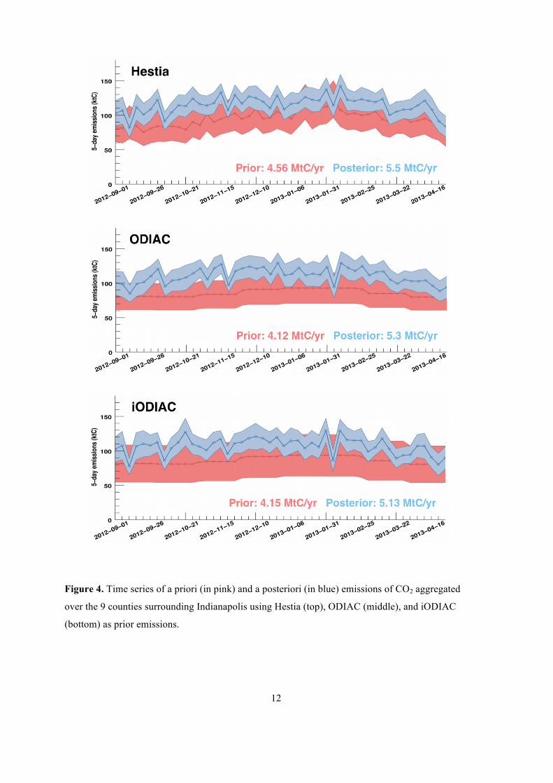
In Figure 4, the temporal variations in the posterior emissions are shown. As shown in

previous inversion cases by Lauvaux et al. (2016), atmospheric data constrain the temporal

variability while prior emissions have no significant impact on the inverse 5-day variations. The

inverse results confirm that while spatial information remains a limiting factor despite the large

number of towers over the city, temporal variations in the emissions being primarily constrained

by observations rather than a priori information. Therefore, the lack of diurnal and sub-monthly

variability in iODIAC is overcome by the observational constraint. This result is discussed further

in Section 4.3 with potential implications for the development of future high resolution EI’s.

12

Figure 4. Time series of a priori (in pink) and a posteriori (in blue) emissions of CO2 aggregated

over the 9 counties surrounding Indianapolis using Hestia (top), ODIAC (middle), and iODIAC

(bottom) as prior emissions.

13

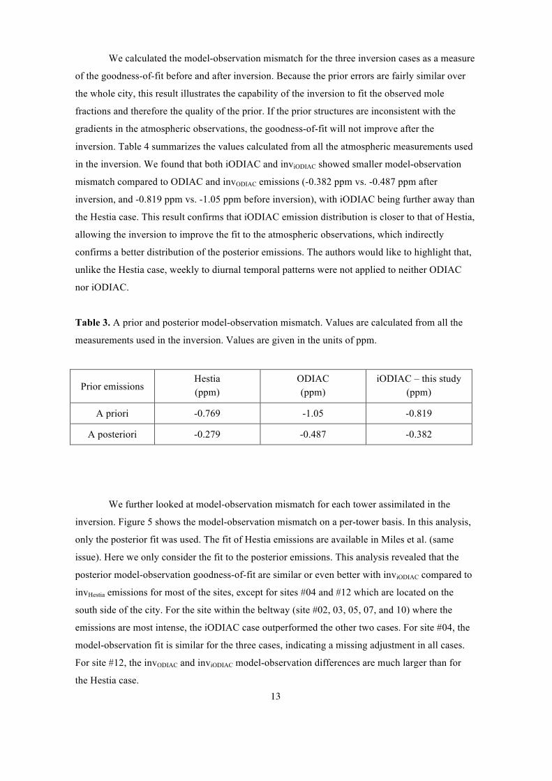
We calculated the model-observation mismatch for the three inversion cases as a measure

of the goodness-of-fit before and after inversion. Because the prior errors are fairly similar over

the whole city, this result illustrates the capability of the inversion to fit the observed mole

fractions and therefore the quality of the prior. If the prior structures are inconsistent with the

gradients in the atmospheric observations, the goodness-of-fit will not improve after the

inversion. Table 4 summarizes the values calculated from all the atmospheric measurements used

in the inversion. We found that both iODIAC and inviODIAC showed smaller model-observation

mismatch compared to ODIAC and invODIAC emissions (-0.382 ppm vs. -0.487 ppm after

inversion, and -0.819 ppm vs. -1.05 ppm before inversion), with iODIAC being further away than

the Hestia case. This result confirms that iODIAC emission distribution is closer to that of Hestia,

allowing the inversion to improve the fit to the atmospheric observations, which indirectly

confirms a better distribution of the posterior emissions. The authors would like to highlight that,

unlike the Hestia case, weekly to diurnal temporal patterns were not applied to neither ODIAC

nor iODIAC.

Table 3. A prior and posterior model-observation mismatch. Values are calculated from all the

measurements used in the inversion. Values are given in the units of ppm.

Prior emissions Hestia (ppm)

ODIAC (ppm)

iODIAC – this study (ppm)

A priori -0.769 -1.05 -0.819

A posteriori -0.279 -0.487 -0.382

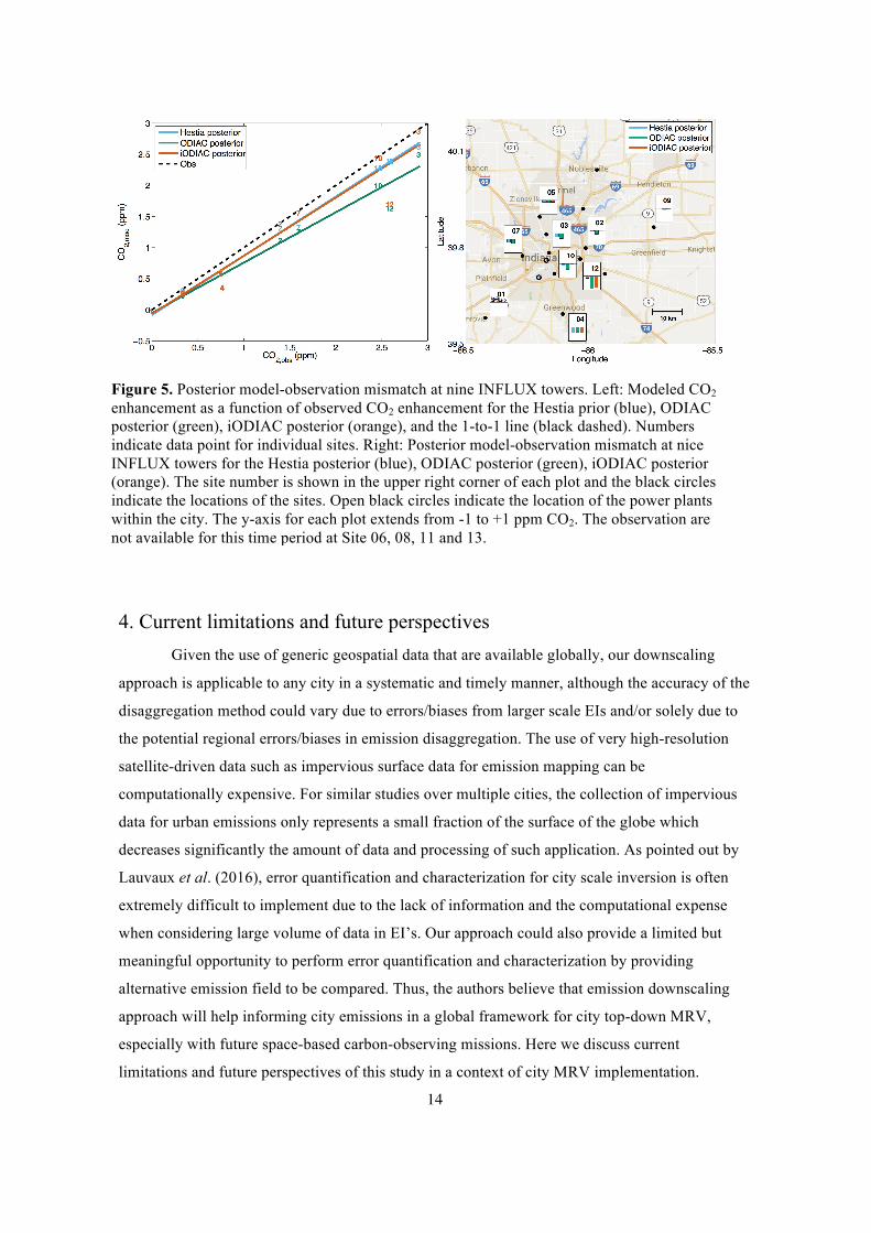
We further looked at model-observation mismatch for each tower assimilated in the

inversion. Figure 5 shows the model-observation mismatch on a per-tower basis. In this analysis,

only the posterior fit was used. The fit of Hestia emissions are available in Miles et al. (same

issue). Here we only consider the fit to the posterior emissions. This analysis revealed that the

posterior model-observation goodness-of-fit are similar or even better with inviODIAC compared to

invHestia emissions for most of the sites, except for sites #04 and #12 which are located on the

south side of the city. For the site within the beltway (site #02, 03, 05, 07, and 10) where the

emissions are most intense, the iODIAC case outperformed the other two cases. For site #04, the

model-observation fit is similar for the three cases, indicating a missing adjustment in all cases.

For site #12, the invODIAC and inviODIAC model-observation differences are much larger than for

the Hestia case.

14

Figure 5. Posterior model-observation mismatch at nine INFLUX towers. Left: Modeled CO2 enhancement as a function of observed CO2 enhancement for the Hestia prior (blue), ODIAC posterior (green), iODIAC posterior (orange), and the 1-to-1 line (black dashed). Numbers indicate data point for individual sites. Right: Posterior model-observation mismatch at nice INFLUX towers for the Hestia posterior (blue), ODIAC posterior (green), iODIAC posterior (orange). The site number is shown in the upper right corner of each plot and the black circles indicate the locations of the sites. Open black circles indicate the location of the power plants within the city. The y-axis for each plot extends from -1 to +1 ppm CO2. The observation are not available for this time period at Site 06, 08, 11 and 13.

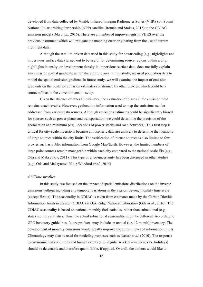
4. Current limitations and future perspectives Given the use of generic geospatial data that are available globally, our downscaling

approach is applicable to any city in a systematic and timely manner, although the accuracy of the

disaggregation method could vary due to errors/biases from larger scale EIs and/or solely due to

the potential regional errors/biases in emission disaggregation. The use of very high-resolution

satellite-driven data such as impervious surface data for emission mapping can be

computationally expensive. For similar studies over multiple cities, the collection of impervious

data for urban emissions only represents a small fraction of the surface of the globe which

decreases significantly the amount of data and processing of such application. As pointed out by

Lauvaux et al. (2016), error quantification and characterization for city scale inversion is often

extremely difficult to implement due to the lack of information and the computational expense

when considering large volume of data in EI’s. Our approach could also provide a limited but

meaningful opportunity to perform error quantification and characterization by providing

alternative emission field to be compared. Thus, the authors believe that emission downscaling

approach will help informing city emissions in a global framework for city top-down MRV,

especially with future space-based carbon-observing missions. Here we discuss current

limitations and future perspectives of this study in a context of city MRV implementation.

15

4.1 Emission information

As pointed out earlier, the lack of EI reported by cities is a fundamental, limiting factor in

city MRV. Although the authors believe that development of a fine-grained EI such as Hestia is

an ideal way to accurately quantify city emissions and inform top down methods in a city MRV

framework, emission accounting for cities via compilation of EIs needs to be more commonly

available and following existing guidelines, such as the Global Protocol for Community-Scale

Greenhouse Gas Emission Inventories (GPC, http://www.ghgprotocol.org/city-accounting). With

sector-specific information, more accurate emission modeling can be implemented instead of

making crude assumptions about sectoral contributions (e.g., applying national-level sectoral

distributions or averaged city sectoral fractions to every city). Spatially defined EIs or geolocation

information will also greatly support the introduction of the complexity and the diversity of

anthropogenic sources in the resulting emission field at fine scale.

The quality of EI is often correlated with the goodness of statistical data collected from

various institutions or directly from private organizations (e.g., Olivier and Peters 2002; Marland,

2008; Andres et al., 2012). Most of the countries that are thought to be producing lower quality

EIs are unlikely to be able to compile high-accuracy EIs at the city scale. Collecting accurate data

at large scales for aggregated EIs (e.g., national and province levels) remains more practical than

city-scale emissions. Therefore, the construction of fine-grained top down estimates to support

city-scale EIs is an attractive solution to produce more accurate estimates in any country, and

possibly offer a monitoring of the reported emissions, consistent with estimates from larger

scales. As an example, Guan et al. (2012) reported a 1Gt CO2 difference between estimates based

on national and province level statistics in China.

4.2 Disaggregation (Mapping) error

Initially, the agreement between ODIAC and Hestia total emissions suggests that the

downscaling approach can give us a reasonable estimate for whole-city emissions (within 10%).

However, disaggregation (mapping) error can be more significant when moving to higher spatial

resolutions. Especially at very high spatial resolution, source locations have to be determined

rather than estimated or approximated using proxy data. As seen in the emission pattern, ODIAC

provides maps of CO2 emissions over areas that are unlikely to be emitting (see Figure 2). Other

than the resolution mismatch (1km vs. 30m), the underlying nightlight data used in ODIAC,

provided by the Defense Meteorological Satellite Program (DMSP) Operational Linescan System

(OLS) nightlight data (https://ngdc.noaa.gov/eog/dmsp.html), have known limitations (e.g.,

Elvidge et al., 2013). The authors are working on applying new nightlight environmental product

16

developed from data collected by Visible Infrared Imaging Radiometer Suites (VIIRS) on Suomi

National Polar-orbiting Partnership (NPP) satellite (Román and Stokes, 2015) to the ODIAC

emission model (Oda et al., 2016). There are a number of improvements in VIIRS over the

previous instrument which will mitigate the mapping error originating from the use of current

nightlight data.

Although the satellite-driven data used in this study for downscaling (e.g., nightlights and

impervious surface data) turned out to be useful for determining source regions within a city,

nightlights intensity, or development density in impervious surface data, does not fully explain

any emission spatial gradients within the emitting area. In this study, we used population data to

model the spatial emission gradient. In future study, we will examine the impact of emission

gradients on the posterior emission estimates constrained by other proxies, which could be a

source of bias in the current inversion setup.

Given the absence of other EI estimates, the evaluation of biases in the emission field

remains unachievable. However, geolocation information used to map the emissions can be

addressed from various data sources. Although emissions estimates could be significantly biased

for sources such as power plants and transportation, we could determine the precision of the

geolocation at a minimum (e.g., locations of power stacks and road networks). This first step is

critical for city-scale inversions because atmospheric data are unlikely to determine the locations

of large sources within the city limits. The verification of intense sources is also limited to few

proxies such as public information from Google Map/Earth. However, the limited numbers of

large point sources remain manageable within each city compared to the national scale EIs (e.g.,

Oda and Maksyutov, 2011). This type of error/uncertainty has been discussed in other studies

(e.g., Oda and Maksyutov, 2011; Woodard et al., 2015)

4.3 Time profiles

In this study, we focused on the impact of spatial emissions distributions on the inverse

emissions without including any temporal variations in the a priori beyond monthly time scale

(except Hestia). The seasonality in ODIAC is taken from estimates made by the Carbon Dioxide

Information Analysis Center (CDIAC) at Oak Ridge National Laboratory (Oda et al., 2016). The

CDIAC seasonality is based on national monthly fuel statistics, rather than subnational (e.g.,

state) monthly statistics. Thus, the actual subnational seasonality might be different. According to

GPC inventory guidelines, future products may include an annual (i.e. 12 month) inventory. The

development of monthly emissions would greatly improve the current level of information in EIs.

Climatology may also be used for modeling purposes such as Nassar et al. (2010). The response

to environmental conditions and human events (e.g., regular weekday/weekends vs. holidays)

should be detectable and therefore quantifiable, if applied. Overall, the authors would like to

17

highlight that the inversion with iODIAC was able to show a very good match with the

atmospheric observations comparable to Hestia inversion case over an 8-month period. Future

work will aim to assess the impact of temporal profiles in the emissions relative to the impact of

finer spatial distributions.

4.4 Error specification

The lack of the error quantification/characterization in the fine-grained emission dataset

was discussed by Lauvaux et al. (2016). As mentioned earlier, many sources of uncertainties can

affect the emissions and need to be carefully considered depending on the flux resolution (e.g.,

time and space) of interest. Most of the emission datasets are based on disaggregation of

emissions (e.g., CDIAC, EDGAR) where proxy data are used at many different levels. The proxy

data are used to approximate the spatial emissions and thus are usually not appropriate at urban

scales where individual processes are identifiable. Emission intercomparison may not be highly

meaningful but given the lack of physical measurements or EIs constructed at comparable spatial

resolutions, model intercomparison remains valid. In the current inversions, the absence of

definition for emissions errors is critical, impairing the ability of top down methods (Lauvaux et

al., 2016). Given the relatively good performance of iODIAC and the presence of detailed spatial

structures, the assessment of emissions errors is a critical objective for urban inversions to

improve both the distribution and the total emissions of the city.

5. Conclusions

We present the first space-based emission field at fine resolution to inform a top-down

urban-scale framework. Following the INFLUX inversion case with a global 1×1 km ODIAC

fossil fuel CO2 emission dataset as a prior, we further improved the 1×1 km emission field from

the global ODIAC dataset to describe higher levels of emission granularity at the city-scale such

as roads and point sources, often missing in coarser resolution products. We approached city

emission fields with three types of geometrical objects to represent the principal emission sector

components: point, line and diffused (area) emission sources. While preserving the point source

information in the ODIAC dataset, we disaggregated the non-point source emissions using

geospatial dataset such as global road network data and satellite-data driven surface

imperviousness data to generate a 30×30 m resolution emission field, comparable to the spatial

scale of Hestia. Our disaggregation theoretically can be applied to any global cities and provide

an emission estimate with spatial distributions even EI are not compiled locally. The posterior

emission estimate summed over the whole city was about 5.1 MtC/yr and remains statistically

similar to the previous inversion using ODIAC (5.3MtC/yr, as reported by Lauvaux et al., 2016).

However, the inversion with the 30×30 m emission field yielded flux corrections with major

18

spatial patterns matched with those of the inverse using a state-of-the-art building-level emission

product, and the optimized model-observation mismatches were similar across the city despite the

absence of hourly variability in the prior emissions.

Although emission disaggregation is not often the best approach to inform emissions at a

high spatial resolution, our result showed that the use of the geospatial data allowed us to improve

the prior emission spatial structure within the city and the potential for providing city emissions

where fine-grained emissions data are not available. Beyond the simple mapping of GHG

emissions, we quantify here the indirect gain of information by using better-informed a priori

emissions, further increasing the potential of the top down approach. This combined approach is

particularly useful as fine-grained emission products like Hestia are rarely available for a vast

majority of the large metropolitan areas across the globe. Currently, city scale emissions are

reported for some cities within local climate action such as Compact of Mayors

(https://www.compactofmayors.org/). If we were to start with such activities using atmospheric

information, the reported EI (often without spatial distributions) needs to be disaggregated, in

order to be incorporated into models. Our method offers a potential approach to a global

verification system of city emissions (MRV) using a disaggregation method and an atmospheric

inversion system at the urban scale. Given the availability of generic geospatial data, our

approach could provide fine-scale city emissions in various locations as future CO2 observations

from ground-based or space missions become more systematically available.

References

Andres RJ, Gregg JS, Losey L, Marland G, Boden TA. 2011. Monthly, global emissions of

carbon dioxide from fossil fuel consumption, Tellus 63B: 309-327.

Andres RJ, Boden TA, Bréon F-M, Ciais P, Davis S, et al. 2012. A synthesis of carbon dioxide

emissions from fossil-fuel combustion, Biogeosciences 9, 1845-1871. doi:10.5194/bg-9-1845-

2012.

Andres RJ, Boden TA, Higdon DM. 2016. Gridded uncertainty in fossil fuel carbon dioxide

emission maps, a CDIAC example, Atmos. Chem. Phys. 16, 14979-14995. doi:10.5194/acp-

16-14979-2016.

19

Asefi-Najafabady S, Rayner PJ, Gurney KR, McRobert A, Song Y. et al. 2014. A multiyear,

global gridded fossil fuel CO2 emission data product: Evaluation and analysis of results. J.

Geophys. Res. Atmos. 119, 10213–10231. doi:10.1002/2013JD021296.

Bovensmann H, Buchwitz M, Burrows, JP, Reuter, M, Krings, T. et al. 2010. A remote sensing

technique for global monitoring of power plant CO2 emissions from space and related

applications. Atmos. Meas. Tech. 3: 781-811.

Buchwitz M, Reuter M, Bovensmann H, Pillai D, Heymann J. et al. 2013. Carbon Monitoring

Satellite (CarbonSat): assessment of atmospheric CO2 and CH4 retrieval errors by error

parameterization. Atmos. Meas. Tech. 6: 3477-3500, doi:10.5194/amt-6-3477-2013.

Center for International Earth Science Information Network - CIESIN - Columbia University, and

Information Technology Outreach Services - ITOS - University of Georgia. 2013. Global

Roads Open Access Data Set, Version 1 (gROADSv1). Palisades, NY: NASA Socioeconomic

Data and Applications Center (SEDAC). http://dx.doi.org/10.7927/H4VD6WCT.

Deng A, Stauffer D, Gaudet B, Dudhia J, Bruyere C. et al. 2009. Update on WRF-ARW end-to-

end multi-scale FDDA system. 10th WRF User’s workshop, NCAR. Boulder, C.O. 14pp.

Duren RM and Miller CE. 2012. Measuring the Carbon Emissions of Megacities. Nature Climate

Change 2: 560–562, doi:10.1038/nclimate1629.

Eldering A. 2015. The OCO-3 Mission: Overview of Science Objectives and Status, 2015

American Geophysical Union (AGU) Fall Meeting, San Francisco.

Elvidge CD, Baugh K, Zhizhin M, Hsu FC. 2013. Why VIIRS data are superior to DMSP for

maping nighttime lights, Proc. the Asia-Pacific Advanced Network 35: 62-69,

http://dx.doi.org/10.7125/APAN.35.7

Enting IG, Trudinger CM and Francey RJ. 1995. A synthesis inversion of the concentration and

d13C atmospheric CO2, Tellus B 47: 35–52.

Feng S, Lauvaux T, Newman S, Rao, P., Ahmadov, R. et al. 2016. Los Angeles megacity: a high-

resolution land–atmosphere modelling system for urban CO2 emissions, Atmos. Chem. Phys.,

16, 9019-9045, doi:10.5194/acp-16-9019-2016.

20

Gately CK, Hutyra LR, Sue Wing I. 2015. Cities, traffic, and CO2: A multi-decadal assessment of

trends, drivers, and scaling relationships. Proc. Natl. Acad. Sci. USA. 112 (16) 4999-

5004. doi: 10.1073/pnas.1421723112.

Guan D, Liu Z, Geng Y, Lindner S, Hubacek K. 2012. The gigatonne gap in China’s carbon

dioxide inventories. Nature Climate Change 2: 672–675.

Gurney KR, Mendoza D, Zhou Y, Fischer M, de la Rue du Can S, Geethakumar S. et al. 2009.

The Vulcan Project: High resolution fossil fuel combustion CO2 emissions fluxes for the

United States. Environment Science and Technology 43: 5535–5541.

Gurney K, Razlivanov I, Song Y, Zhou Y. et al. 2012. Quantification of fossil fuel CO2 emission

on the building/street scale for a large US city. Environ. Sci. & Technol. 46: 12194-12202.

Gurney KR, Liang J, Patarasuk R, O’Keeffe D, Huang J. et al. 2016. Reconciling the differences

between a bottom-up and inverse-estimated FFCO2 emissions estimate in a large US urban

area, submitted to Elementa

Hutyra L, Duren R, Gurney KR, Grimm N, Kort E. et al. 2014. “Urbanization and the carbon

cycle: Current capabilities and research outlook from the natural sciences

perspective”, Earth’s Future, doi:10.1002/2014EF000255.

Janardanan R, Maksyutov S, Oda T, Saito M, Kaiser JW, Ganshin A, Stohl A, Matsunaga T,

Yoshida Y, Yokota T. 2016. Comparing GOSAT observations of localized CO2 enhancements

by large emitters with inventory-based estimates, Geophys. Res. Lett. 43,

doi:10.1002/2016GL067843.

Janssens-Maenhout G, Dentener F, Van Aardenne J, Monni S, Pagliari V, et al. 2012. EDGAR-

HTAP: a Harmonized Gridded Air Pollution Emission Dataset Based on National Inventories.

Ispra (Italy): European Commission Publications Office; 2012. JRC68434, EUR report No

EUR 25 299 - 2012, ISBN 978-92-79-23122-0, ISSN 1831-9424

Kort EA, Frankenberg C, Miller CE, Oda T. 2012. Space-based observations of megacity carbon

dioxide. Geophys. Res. Lett. 39: 17-22.

21

Kuenen J, Visschedijk A, Jozwicka M, Gon H. 2014. TNO-MACC_II emission inventory; a

multi-year (2003– 2009) consistent high-resolution European emission inventory for air

quality modelling, Atmos Chem Phys, 14(20), 10963–10976, doi:10.5194/acp-14-10963-2014.

Kurokawa J, Ohara T, Morikawa T, Hanayama S, Janssens-Maenhout G. et al. 2013. Emissions

of air pollutants and greenhouse gases over Asian regions during 2000–2008: Regional

Emission inventory in ASia (REAS) version 2, Atmos. Chem. Phys. 13: 11019-11058,

doi:10.5194/acp-13-11019-2013.

Lauvaux T. et al. 2016. High-resolution atmospheric inversion of urban CO2 emissions during the

dormant season of the Indianapolis Flux Experiment (INFLUX), J. Geophys. Res.

Atmos., 121, doi:10.1002/2015JD024473.

Liu Z. et al. 2015. Reduced carbon emission estimates from fossil fuel combustion and cement

production in China, Nature 524: 335–8

Marland G. 2008. Uncertainties in Accounting for CO2 From Fossil Fuels. J. Industrial Ecology,

12: 136–139. doi: 10.1111/j.1530-9290.2008.00014.x.

Miles NL. et al. 2016. Detectability and quantification of atmospheric boundary layer greenhouse

gas dry mole fraction enhancements in an urban landscape: Results from the Indianapolis Flux

Experiment (INFLUX) submitted to Elementa

Mills G. 2007. Cities as agents of global change. International Journal of Climatol. 27: 1849-

1857.

Nassar R, Jones DBA, Suntharalingam P, Chen JM, Andres RJ. et al. 2010. Modeling global

atmospheric CO2 with improved emission inventories and CO2 production from the oxidation

of other carbon species. Geosci. Model Dev. 3: 689-716.

Nisbet E. and Weiss R. 2010. Top-down versus bottom-up, Science 328: 1241–1243. doi:

10.1126/science.1189936.

Oda T and Maksyutov S. 2011. A very high-resolution (1km×1km) global fossil fuel CO2

emission emission inventory derived using a point source database and satellite observations

of nighttime lights. Atmos. Chem. and Phys. 11: 543-556.

22

Oda T, Maksyutov S, Andres RJ. 2016. The Open-source Data Inventory for Anthropogenic CO2

(ODIAC) fossil fuel emission model version 3.0 (ODIAC v3.0), submitted to Geosci. Model

Dev.

Olivier JGJ. 2002. On the Quality of Global Emission Inventories: Approaches, Methodologies,

Input Data and Uncertainties, PhD thesis University Utrecht, ISBN 90-393-3103-0

Olivier JGJ, Aardenne JAV, Dentener FJ, Pagliari V, Ganzeveld LN, Peters JAHW. 2005. Recent

trends in global greenhouse gas emissions: Regional trends 1970–2000 and spatial distribution

of key sources in 2000, J. Integr. Env. Sci. 2: 81–99. doi:10.1080/15693430500400345.

Olivier JGJ. and Peters JAHW. 2002. Uncertainties in global, regional, and national emissions

inventories. In Non-CO2 greenhouse gases: Scientific understanding, control options and

policy aspects, edited by: Van Ham J, Baede APM, Guicherit R, and WIlliams-Jacobse JFGM,

Springer, New York, USA, 525–540.

Pacala SW. et al. 2010. Verifying Greenhouse Gas Emissions: Methods to Support International

Climate Agreements. Committee on Methods for Estimating Greenhouse Gas Emissions;

National Research Council, National Academy of Sciences, 124pp.

Patarasuk P, Gurney KR, O’Keeffe D, Song Y. Huang J. et al. 2016. Application of high-

resolution fossil fuel CO2 emissions quantification to urban climate policy in Salt Lake

County, Utah USA, Urban Ecosystems. DOI 10.1007/s11252-016-0553-1.

Polonsky IN, O'Brien DM, Kumer JB, O'Dell CW. and the geoCARB Team:. 2014. Performance

of a geostationary mission, geoCARB, to measure CO2, CH4 and CO column-averaged

concentrations, Atmos. Meas. Tech. 7: 959-981, doi:10.5194/amt-7-959-2014.

Rayner PJ, Raupach MR, Paget M, Peylin, P, Koffi E. 2010. A new global gridded data set of

CO2 emissions from fossil fuel combustion: Methodology and evaluation. J. Geophys. Res.

115, D19306, doi:10.1029/2009JD013439.

Richardson SJ, Miles NL, Davis KJ, Lauvaux L, Martins DK. et al. 2016. CO2, CH4, and CO

tower in situ measurement network in support of the Indianapolis FLUX (INFLUX)

Experiment. submitted to Elementa

23

Román MO and Stokes EC. 2015. Holidays in Lights: Tracking cultural patterns in demand for

energy services. Earth’s Future. doi:10.1002/2014EF000285.

Streets D. et al. 2003. An inventory of gaseous and primary aerosol emissions in Asia in the year

2000, J. Geophys. Res., 108(D21), 8809, doi:10.1029/2002JD003093.

Turnbull JC. et al. 2015. Toward quantification and source sector identification of fossil fuel CO2 emissions from an urban area: Results from the influx experiment. J. Geophys. Res. Atmos.

120: 292–312, doi:10.1002/2014JD022555.

Uliasz M. 1994. Lagrangian particle modeling in mesoscale applications, in Environmental

Modelling II, edited by P. Zanetti, Computational Mechanics Publications, pp.71–102.

Woodard D, Branham M, Buckingham G, Hogue S, Hutchins M. et al. 2014. A spatial

uncertainty metric for anthropogenic CO2 emissions", Greenhouse Gas Measurement and

Management (2014) 2-4, 139-160.

Contributions

TO and TL conceived and designed the study, implemented the analysis and drafted the

manuscript. NLM and SJR acquired atmospheric CO2 data. KRG developed and provided Hestia

emission dataset. PR and DL contributed to geospatial data processing. All the authors

contributed to improve the manuscript.

Acknowledgment The authors would like to thank Junmei Tang for providing her expertise to data processing of

geospatial data.

Funding Information

TO is supported by NASA Carbon Cycle Science program (Grant # NNX14AM76G). TL is

supported by the National Institute for Standards and Technology (INFLUX project

#70NANB10H245) and the National Oceanic and Atmospheric Administration (grant

#NA13OAR4310076).

Competing information

24

The authors have declared that no competing interest exists.

Data accessibility statement The ODIAC global emission dataset is available at

http://db.cger.nies.go.jp/dataset/ODIAC/. “Hestia” fine-grained emission dataset is avaialbe from

http://hestia.project.asu.edu/. The Global Roads Open Access Data Set (gROADS) v1 is available

from http://sedac.ciesin.columbia.edu/data/set/groads-global-roads-open-access-v1. National

Land Cover Dataset (NLCD) 2011 is available from http://www.mrlc.gov/nlcd2011.php. The

atmospheric CO2 tower data used in this study are available at http://sites.psu.edu/influx/data/.