NBER WORKING PAPER SERIES

ON THE HETEROGENEITY OF DOWRY MOTIVES

Raj ArunachalamTrevon D. Logan

Working Paper 12630http://www.nber.org/papers/w12630

NATIONAL BUREAU OF ECONOMIC RESEARCH1050 Massachusetts Avenue

Cambridge, MA 02138October 2006

We are grateful for helpful comments from Pranab K. Bardhan, Chang-Tai Hsieh, Jennifer Johnson-Hanks,Lung-Fei Lee, Ronald D. Lee, David I. Levine, Ian McLean, Manisha Shah, and seminar participantsat UC Berkeley and Ohio State University. We would particularly like to thank J. Bradford DeLong,Audrey L. Light, and Edward Miguel for several useful discussions and encouragement throughout.Hao Shi and Ranjan Shrestha provided excellent research assistance. Corresponding author: Raj Arunachalam,Department of Economics, University of California, Berkeley, 549 Evans Hall #3880, Berkeley, CA94720-3880. Email: arunacha@econ.berkeley.edu The views expressed herein are those of the author(s)and do not necessarily reflect the views of the National Bureau of Economic Research.

© 2006 by Raj Arunachalam and Trevon D. Logan. All rights reserved. Short sections of text, notto exceed two paragraphs, may be quoted without explicit permission provided that full credit, including© notice, is given to the source.

On the Heterogeneity of Dowry MotivesRaj Arunachalam and Trevon D. LoganNBER Working Paper No. 12630October 2006JEL No. C5,D1,J12

ABSTRACT

Dowries have been modeled as pre-mortem bequests to daughters or as groom-prices paid to in-laws.These two classes of models yield mutually exclusive predictions, but empirical tests of these predictionshave been mixed. We argue that the heterogeneity of findings can be explained by a heterogeneousworld--some households use dowries as a bequest and others use dowries as a price. We estimate amodel with heterogeneous dowry motives and use the predictions from the competing theories in anexogenous switching regression to place households in the price or bequest regime. Our empiricalstrategy generates multiple, independent checks on the validity of regime assignment. Using retrospectivemarriage data from rural Bangladesh, we find robust evidence of heterogeneity in dowry motives inthe population; that bequest dowries have declined in prevalence and amount over time; and that bequesthouseholds are better off compared to price households on a variety of welfare measures.

Raj Arunachalam University of California, BerkeleyDepartment of Economics549 Evans Hall #3880Berkeley, CA 94720-3880arunacha@econ.berkeley.edu

Trevon D. LoganThe Ohio State University410 Arps Hall1945 North High StreetColumbus, OH 43210and NBERlogan.155@osu.edu

1 Introduction

In the last decade a sharp debate has emerged over the predominance of dowry in

South Asia. With the historical knowledge that dowries tend to disappear as societies

modernize, the persistence of substantial bride-to-groom marriage transfers has long

been a puzzle for social scientists. Recently, in the wake of increasingly male-favored

sex ratios, and with dowries in South Asia currently representing upwards of several

multiples of a bride’s family’s annual income (Suran, Amin, Huq, and Chowdury,

2004; Rao, forthcoming), accounting for dowry has attained a new urgency for scholars

and policy-makers alike. Attempts to explain this puzzle have centered on the very

understanding of what dowry represents: a price or a bequest.

First formalized by Becker (1981), the price model sees dowries as transfers be-

tween families, in which brides do not directly benefit. Such transfers may be neces-

sary for a number of reasons. Cultural factors such as hypergamy (women marrying

“up” the social ladder) or tendency for brides to marry older men (in the context

of population growth) may create a perpetual scarcity of grooms, such that dowry

emerges to draw high-quality men into the marriage market (Rao, 1993; Anderson,

2003). Else, if rules for division of household output are inflexible, and a woman’s

shadow price in the marriage market exceeds her share of income, dowry will emerge

as an upfront transfer to equilibriate the marriage market (Botticini and Siow, 2003).

Finally, greater heterogeneity in market earnings among men than among women may

produce dowry as a mechanism by which brides attract high-quality grooms (Ander-

son, 2004). Regardless of their differences, these explanations share one feature: they

are grounded in a model of dowry as a price that clears the marriage market.

A competing set of answers to the dowry puzzle, only recently formalized in the

economics literature, views dowry as bequests, in which parents transfer their inheri-

tance to daughters at the time of marriage. If there are institutional or legal barriers to

women’s ability to inherit property, particularly in virilocal societies (where daughters

leave their natal household at marriage), dowry may emerge as a culturally-sanctioned

method of bequest (Zhang and Chan, 1999). Alternatively, in virilocal societies, a

pre-mortem bequest to daughters may emerge as a method of maintaining sons’ in-

centive to exert full effort in maintaining their parents’ estate (Botticini and Siow,

2003). Finally, if such societies are marked by poor protection of women in their

in-laws’ households, dowry may improve brides’ outside option in a bargaining set-

2

ting, and thus mitigate the incidence of domestic violence and other forms of abuse

(Brown, 2003). All of these explanations view dowry as a transfer to the daughter,

and under her control, at the time of marriage.

The policy implications of this debate are critical: if dowries are bequests, they

should be protected, as they represent culturally-sanctioned access to property for

women (Kishwar, 1989; Goody, 1998). More generally, dowry as bequest can improve

brides’ consumption within in-laws’ households, thereby improving women’s welfare.

If dowries are a groom-price, the practice of dowry should arguably be banned, par-

ticularly in South Asia, as it increases the perceived cost of raising daughters and

thus may contribute to worsening sex ratios through selective abortion, infanticide,

and differential child mortality by gender. To date, bans of dowry have taken the

form of largely ineffectual “paper laws,” but momentum is gaining among activists

and policy-makers to make the prohibition of dowries bite, by publicizing regulations,

increasing the penalties for violations, and making reporting to authorities more at-

tractive (Setalvad, 1988; Menski, 1998; Basu, 2005).

With the stakes set so high, the empirical evidence is mixed. To date, no large-

sample survey in South Asia directly asks respondents to identify the recipient of

the dowry transfer, since groom-prices are technically banned. Researchers must

therefore use indirect measures to assess the function of dowry. Such indirect tests,

in South Asia and elsewhere, have yielded contrary results, sometimes within the

same paper (see Table 1). Meanwhile, drawing on village case studies, historians and

anthropologists have argued that the system of dowry in India and Bangladesh has

transformed over the recent decades from bequest to price—yet their reliance on small

samples and sparse archival records renders the generalizability of such conclusions

suspect (Lindenbaum, 1981; Ahmed and Naher, 1987; Sharma, 1984).

We propose a simple explanation for the mixed results in the literature: hetero-

geneity in dowry motives, and develop a theoretical and empirical strategy to deal

with this heterogeneity. All prior large-sample studies take a particular model of

dowry as given, regress dowry amounts on bride, groom and marriage market char-

acteristics, and infer support for the model from the sign of estimated coefficients on

theoretically “important” variables. In the presence of heterogeneity, however, such

a strategy is misguided, precisely because average coefficients are uninformative as

to the actual functioning of dowry. By acknowledging instead that both models may

hold—for different subsets of the population—we use their theoretical predictions to

3

structure a switching regression model with unknown sample separation to sort the

marriage market into “bequest households” and “price households.” More precisely,

we use the theories to help predict households’ probability of regime membership and

estimate a probability-weighted dowry function for each regime.

There are four central findings. First, using retrospective data from the 1996

Matlab Health and Socioeconomic Survey, we find substantial evidence of two dowry

regimes in rural Bangladesh. In particular, of marriages from 1920 to the present in

which a dowry was given, more than a quarter used dowry as bequest. Second, the

function mapping bride household, groom household, and marriage market charac-

teristics to dowry amounts (the dowry function) differs significantly between regimes.

Third, dowries increasingly serve as a groom-price, and while bequest dowries are

falling in size, price dowries are rising. We fail, however, to find evidence of a “mar-

riage squeeze” driving dowry inflation. Finally, bequest households are considerably

better off—in schooling, assets, and other measures of welfare—than price households.

Beyond its contribution to the literature on dowries, our paper presents a general

methodology that can be fruitfully adopted in other debates where there is more than

one model and no clear victor. We offer three methodological advances on similar

papers which proactively use theory in a switching regression framework in order

to locate sources of heterogeneity.1 First, rather than rely on a single characteris-

tic as the predictor of regime membership, we utilize a number of predictions from

the competing theories—thus enabling each estimate to serve as a validity check on

the others. Second, we generate a novel type of prediction of regime membership:

a “non”-membership prediction, which indicates the likelihood that an observation

does not fall within a given regime. As such, we offer a new method of classifying

regime membership which may be more readily derived from economic models than

“membership” predictions. Finally, employing these non-membership predictions (in

the switching equation) as well as predictions regarding regime specifications (in the

regime equations) allows us multiple robustness checks by relaxing different assump-

tions. Our strategy may prove of interest in areas as wide-ranging as unitary vs.

non-income-pooling households, separability vs. non-separability of household pro-

duction and consumption, strategic vs. altruistic bequests, and the permanent income

1Two recent examples of this approach are Kopczuk and Lupton (forthcoming), which investigatesheterogeneity in bequest motives of the elderly, and Vakis, Sadoulet, de Janvry, and Cafiero (2004),which looks at heterogeneity in the separability of household consumption from production.

4

hypothesis, by offering empirical researchers new strategies for using theory to locate

sources of heterogeneity.

2 Two Theories of Dowry

In this section we reformulate existing price and bequest theories in a framework

that highlights the salient distinctions between the two classes of models, and extract

predictions for regime membership which we exploit in the empirical analysis.

2.1 Price Model

Since Becker (1981) broke open the economic modeling of marriage payments and

offered the first formal statement of the price model, a number of authors have de-

veloped various theoretical predictions for aspects and effects of dowries (Rao, 1993;

Grossbard-Shechtman, 1993; Sen, 1998; Mukherjee, 2003; Dasgupta and Mukherjee,

2003; Anderson, 2003, 2004; Dalmia, 2004; Tertilt, 2005; Mukherjee and Mondal,

2006). The model presented below highlights the shared properties of these models

while generating a number of useful predictions which we take to the data. The crit-

ical feature of price models, for our purposes, is that the dowry is transferred from

the bride’s family to the groom’s family to equilibriate the marriage market. As such,

the model yields a dowry function that maps characteristics of the bride, groom, and

their respective families, as well as underlying features of the marriage market, to a

dowry amount.

Marriage decisions are made by the parents (the “family”) of each spouse. Each

family chooses a spouse for their child to maximize utility. The groom’s family

(indexed by G) has utility UG = UG(cG, wS, wD), where cG is parental consump-

tion and wS is the son’s wealth. The groom’s parents choose wD, the wealth of

their desired daughter-in-law, to maximize utility subject to the budget constraint

cG = wG + τ(wD; wS, R), taking wG (the groom’s parents’ pre-transfer wealth), wS,

R, and τ(·) as given. R is a shifter of the dowry function that is not related to the

individual bride or groom’s household (for example, sex ratio, year of marriage, re-

gion, etc.). Here, τ(·) is a function mapping each prospective bride to a transfer that

sustains the match, given wS and R. The solution to this problem yields a schedule

5

of transfers, DG, that sustain each bride-groom pairing acceptable to the groom’s

parents (analogous to an inverse demand function): DG = DG(wD, wS, wG, R). The

bride’s family (indexed by P ) faces a similar problem, except that they pay the trans-

fer. They choose wS to maximize their utility UP = UP (cP , wD, wS) subject to the

budget constraint cP = wP − τ(wS; wD, R), taking wP , wD, R and τ(·) as given.

Again, the solution yields a schedule of transfers that sustain each bride-groom pair-

ing acceptable to the bride’s parents: DP = DP (wD, wS, wP , R).

In equilibrium, the marginal utility of the spouse traits to consumption, for both

bride and groom families, will be equal:

∂UG

∂wD

∂UG

∂cG

=

∂UP

∂wS

∂UP

∂cP

At any given value of R, a bride-groom pairing can only be sustained in equi-

librium when DG = DP . This gives us a dowry function—a schedule mapping each

bride-groom pair to an equilibrium transfer: D∗ = D∗(wD, wS, wP , wG, R). In this

setting, every bride-groom combination is feasible given a transfer of the right amount,

since we have not restricted transfers to be non-negative. Figure 1 demonstrates this

graphically—a woman of wealth wD can match with any man, given the appropriate

dowry.

We now summarize two key predictions of the price model of dowry that we will

use to identify regime membership in the empirical section. First, the dowry that

sustains any particular couple is determined by the characteristics of the bride and

her family (a vector W ), the groom and his family (a vector H), and a vector R of

parameters such as sex ratio that “shift” the dowry function. In reduced form, we

can write:

DΠ = gΠ(H, W, R) (1)

where D is dowry amount, g(·) is the dowry function, and Π indexes the price regime.

Second, we have a non-membership prediction for marriages in the price regime which

should see no dowry transferred:

• DΠ = 0 in a love (or “self-arranged”) marriage.2

2This prediction has a long history in the literature on marriage transfers, going back to Goode(1963) and Becker (1981) and recently discussed by Dasgupta and Mukherjee (2003) and Edlundand Lagerlof (2004). First, and most simply, in a love marriage the selection of the spouse is made

6

Furthermore, a number of authors have made clear predictions about the dowry

function itself. We refer to these as testable predictions—rather than taking them as

given, we will empirically test their substantive significance:

• Ceteris paribus, dowry amount moves inversely with bride’s “positive” char-

acteristics (or “quality”) and positively with groom’s “positive” characteris-

tics. These features may include human capital attainment, ability to make

economic contributions to groom’s household (Becker, 1981; Behrman, Foster,

Rosenzweig, and Vashishtha, 1999), and non-economic characteristics such as

caste (Anderson, 2003). In short, attributes substitute for dowry amount.

• Ceteris paribus, dowry amount moves inversely with the male-to-female sex

ratio (Grossbard-Shechtman, 1993) or age-adjusted sex ratio (Rao, 1993). As

a transfer that equilibriates the marriage market, dowry is a function of excess

supply.

2.2 Bequest Model

The bequest theory does not merely view dowry as an intergenerational transfer—

the idea is that in dowry-giving societies, inheritance is given to a son at the time

of parents’ death but to a daughter upon her marriage. Key to such a model is

the notion that some friction prevents daughters from inheriting upon their parents’

death. Most scholars stress the combination of virilocality and poor property rights:

since women face barriers to inheriting after moving to their in-laws’ household, they

must receive their inheritance at the time of marriage.3

While the bequest explanation has a long tradition in anthropology (Tambiah,

1973, for example), only recently have economists developed the notion that dowry

functions as pre-mortem inheritance into models that can be estimated (Zhang and

Chan, 1999; Edlund, 2001; Botticini and Siow, 2003; Suen, Chan, and Zhang, 2003;

by bride and groom, not by their parents, as the price model requires. Second, such a marriage willnot be under the same market pressures present in the implicit dowry market. Another way to put itis that a model of dowry as price assumes that dowry allows parents of daughters to secure allianceswith high-quality in-laws. Thus, love marriages, where parents are not the decision-makers, shouldsee no dowry transferred.

3Botticini and Siow (2003) maintain the assumption that virilocality is crucial to the existence ofdowry, but posit that parents’ inability to monitor their son’s effort forces them to make an inefficientpre-mortem bequest to their daughter in order to properly incentivize the son’s management of thehousehold estate.

7

Brown, 2003). Of these papers, only Botticini and Siow (2003) develops the idea that

a model of dowry as bequest must be nested within a marriage market—and that

a premarital transfer to their daughter automatically improves the groom she will

attract. We draw from this insight in constructing the model below.

Using subscripts P for bride’s parents, D for the bride, and S for the son-in-law,

the bride’s parents derive utility UP from her marriage such that: UP = U(cP , cD, cS),

a function increasing and concave in all arguments. Here, cP is consumption of the

parents; cD is the “marital wealth” of the daughter (the wealth that she brings into

her marriage), and cS is the marital wealth of the son-in-law. Parents maximize

utility by choosing the size of the dowry transfer τ , which is made to the daughter.

The parental budget constraint is: cP = wP −τ , where wP is the parent’s pre-transfer

wealth, and τ is constrained to be non-negative.4

Now we turn to the daughter. The first key feature of the model is the assumption,

following Lam (1988); Peters and Siow (2002) and Botticini and Siow (2003), that a

bride’s characteristics, such as age, education, and number of siblings, are exogenously

mapped by the marriage market to a scalar which we call “pre-marital wealth”. This

allows us to write: wD = f(XD), where wD is her pre-marital wealth and XD is a

vector of characteristics. This mapping allows us to state the “marital wealth” cD

that the daughter brings into her marriage as: cD = wD + τ .

Finally we consider the son-in-law. The second key feature of the model is that

we nest the choice of dowry amount within a assortative matching framework. Since

brides and grooms can be ranked by marital wealth, each woman of marital wealth

cD attracts a groom of marital wealth cS = h(cD), where the existence of the weakly-

monotonic mapping h(·) follows from assortative mating.5 Substituting, the bride’s

parents choose τ to maximize: UP = U(wP − τ, wD + τ, h(wD + τ)). In the interior,

the optimal τ ∗ gives:

∂U

∂(wP − τ ∗)=

∂U

∂(wD + τ ∗)=

∂U

∂(h(wD + τ ∗))(2)

In addition, the non-negativity constraint on τ yields a possible corner solution τ ∗ = 0.

By the monotonicity of h(·), equation (2) identifies τ ∗. In other words, since

4While we do not formally model the source of the non-negativity constraint on bequests, itarises naturally out of capital market imperfections which prevent daughters from borrowing beforemarriage. Baland and Robinson (2000) make this point in a different context.

5Existence of equilibrium in wealth matching models is shown in Peters and Siow (2002).

8

son-in-law’s marital wealth is simply a function of the daughter’s marital wealth, the

choice of dowry amount will not depend on the son-in-law’s wealth. We can thus write

a schedule of optimal dowry amounts τ ∗ as a function only of parents’ and daughter’s

pre-marital wealth: τ ∗(wP , wD) = τ ∗(wP , f(XD)).

In this setting, unlike in the price model, dowry cannot substitute for groom’s

characteristics. The intuition is straightforward: since the transfer can only be made

to daughters, any attempt to improve parental utility by securing a superior son-in-law

can only occur by improving the daughter’s marital wealth ranking among prospective

brides. We demonstrate this graphically in Figure 2. Vertical axes represent the

marital wealth of brides and grooms. A bride of pre-marital wealth wD will marry

a groom of marital wealth h(wD + τ), where τ is chosen by the bride’s parents to

maximize parental utility, so that the thick line represents the range of possible grooms

a bride may match with.

This result gives us a valuable “reduced-form restriction” which we use in the

estimation:

DB = gB(W ) (3)

where B indexes the bequest regime and gB(•) is the dowry function. That is, the

dowry amount in the bequest regime depends solely on W , the vector of characteristics

of the bride and her family (including XD and wP ). To put it another way, once the

bride’s characteristics and the dowry amount are known, the knowledge of groom’s

characteristics do not add any additional information, and should be excluded from

the estimation.

Furthermore, the logic of the bequest theory yields a number of non-membership

predictions that describe the characteristics of families who will not give a dowry as

bequest:

• DB = 0 if the bride remains within the household after marriage. Virilocality

combined with the cessation of daughters’ ability to inherit drive the pre-mortem

bequest.

• DB = 0 if the bride’s parents have died before her marriage. Again, since

daughters face no barriers to inheritance before moving away, they will have

already inherited.

• DB = 0 if the bride has been previously married, since she will have received

9

her bequest at the time of her first marriage.

• The Botticini and Siow (2003) model offers an additional prediction: DB = 0 if

the brides has no brothers of the age of majority at the time of marriage.6

The bequest theory also offers predictions about the dowry function in this regime:

• Ceteris paribus, dowry amount moves inversely with the bride’s number of

brothers of the age of majority. In the bequest theory, sons do not “attract”

dowry from their in-laws—thus, each brother represents another drain on the

inheritance pool.

• Ceteris paribus, a higher dowry improves the bride’s well-being, both by increas-

ing her marital wealth and by improving the quality of her potential groom.

3 Heterogeneity in Dowry Motives

We argue in this section that the bulk of the historical and anthropological evidence

points toward two models of dowry: bequest and price.7 After a brief discussion of

previous empirical work, highlighting the pitfalls involved in imposing homogeneity of

dowry motive, we provide a simple model which relaxes this assumption. We consider

a bifurcated marriage market in which some unknown fraction of households only use

dowries as bequests (the “bequest regime”), and the rest use dowries as a price (the

“price regime”). This model, grounded in the theoretical predictions stated in the

previous section, serves as the basis for the empirical work that follows.

3.1 Historical and Anthropological Accounts

The earliest reference to dowry in South Asia dates almost two millenia ago—when

Manu decreed stridhan [dowry] to represent the “sixfold property of a woman” (Old-

enburg, 2002). The origins of dowry in South Asia almost certainly lie in a system

6If a bride has no brothers (or if her brothers are below the age of majority at the time of hermarriage), the incentive problem that forces an inefficient pre-mortem bequest is vitiated. Anybequest will be given upon her parents’ death or at the time when any brother reaches the age ofmajority and assumes responsibility for managing the parents’ estate.

7This discussion serves as motivation, but in the empirics we do not require that both regimesexist—on the contrary, the switching regression approach allows us to explicitly test whether thetwo-regime model fits the data better than a single-regime model.

10

of premortem inheritance, but most scholars document a gradual transformation of

dowry from bequest to price beginning sometime in the late nineteenth century (Tam-

biah, 1973; Srinivas, 1984; Banerjee, 1999).8 At any given point in time, however,

there is evidence of heterogeneity of opinion about dowry. Some nineteenth century

observers viewed dowry as an unambiguous bequest: “[I]f the daughter receives some-

thing at the time of her marriage,” a Bengali defender of dowry wrote in 1887, “then

is that not a good thing? When the father is compelled to spend money for his daugh-

ter, and that sum accrues to the in-laws or to the bridegroom, in the ultimate analysis

the daughter is the principal beneficiary” (cited in Majumdar (2004, pgs. 445-446)).

In precisely the same period, critiques of dowry began to proliferate, particularly in

Calcutta, all citing the language of the marketplace to describe the increasing “price”

of grooms (Majumdar, 2004).

Anthropologists’ accounts, generally drawing from long-term fieldwork in a small

number of villages, likewise reflect considerable heterogeneity in dowry motives, both

in the assessment of scholars and in the views of their informants. One anthropologist

who conducted fieldwork in Himachal Pradesh and Punjab during the late 1970s re-

ported that her informants (mostly Hindu) saw dowry as a pre-mortem inheritance to

daughters, yet her own observations led her to conclude that dowry amounts moved as

a price in a marriage market (Sharma, 1984, pg. 351). Another, conducting fieldwork

in the 1980s among urban Protestants in Madras, found that respondents overwhelm-

ingly perceived dowry as a groom-price, noting that dowry amounts fell with aspects

of a bride’s perceived quality (Caplan, 1984).9 As with the historical evidence, an-

thropological accounts almost universally document a transformation of dowry from

bequest to price. This trend is evident in Comilla, the district of Bangladesh from

which our survey data comes. As early as the 1950s, a new form of marriage transfer

emerged in which potential grooms detailed the list of items they would accept in

8Considerable evidence from other dowry-giving societies around the world similarly points tothe coexistence of bequest and price dowries, and the transformation from bequest dowries to pricedowries over time (Kaplan, 1985; Nazzari, 1991).

9Such discussions abound in South Asian literature. For instance, early in Kamala Markandaya’s1954 Nectar in a Sieve, a South Indian mother assesses potential grooms for her daughter: “At lastwe found one who seemed to fulfill our requirements: he was young and well favoured, the only sonof his father from whom he would one day inherit a good portion of land.

‘They will expect a large dowry,’ I said regretfully. ‘One hundred rupees will not win such ahusband, we have no more.’

‘She is endowed with beauty,’ Old Granny said. ‘It will make up for a small dowry—in this case.’” (New York, John Day, pgs. 39-40).

11

exchange for marriage—these payments were often called by the English word “de-

mand,” reflecting the price motive of the dowry (Lindenbaum, 1981; Kabeer, 2001).

Concomitant with the transition in the function of dowry, anthropological work

indicates a change in the form of payment. As bequest dowry declined in prevalence,

dowries increasingly began to be paid in cash, over which brides rarely exercised

control in their in-laws’ household (Sharma, 1984; Caplan, 1984). While the data we

use does not include information about respondents’ control over different types of

dowry, survey data from elsewhere in South Asia support this generalization.10

In sum, a survey of the historical and anthropological evidence on dowry points

not only to heterogeneity of dowry motives, but establishes that there are two (and

only two) predominant explanations for the function of dowry, which correspond to

our price and bequest models. Furthermore, the literature provides two claims we

use as checks to the validity of our empirical results:

• Dowry as bequest has been declining in prevalence over time.

• Dowries as bequests are less likely to be cash-only, since cash is not a resource

over which brides exercise control within the in-laws’ household.

3.2 Previous Empirical Work

Contrary to the evidence presented above, most empirical studies of dowry proceed

by taking either the price or bequest model as given. There are two central problems

with this strategy. First, in the presence of heterogeneity, testing each theory’s pre-

dictions about the specific nature of the dowry function is only feasible once regime

membership has been determined—a point we develop below. Second, tests often

rest on predictions common to both models. Previous tests of the bequest model

adopt a “welfare” approach, focusing on the prediction that ceteris paribus, higher

dowries increase bride’s welfare. Accordingly, the strategy has been to regress mea-

sures of bride’s welfare on dowry amount and a number of controls (Zhang and Chan,

10The Survey on the Status of Women and Fertility in Uttar Pradesh and Tamil Nadu (Smith,Ghuman, Lee, and Mason, 2000) asked randomly-sampled brides about the control they exerciseover different forms of dowry. In marriages where cash dowry was given as dowry, fewer than 10%of respondents reported that they had the “major say” in how the cash was spent, and more than70% reported that they had no say at all. In marriages where jewelry, gold, or silver was given,more than 47% of respondents reported that they had the major say in how it was used or whetherit could be sold, while fewer than 25% reported that they had no say at all.

12

1999; Brown, 2003; Suran, Amin, Huq, and Chowdury, 2004; Esteve-Volart, 2004).11

However, this is not a viable test of the bequest model. Indeed, we generated above

the price model’s prediction that, ceteris paribus, higher dowry attracts higher qual-

ity grooms. If, for example, we accept Zhang and Chan’s (1999) hypothesis that

husbands’ willingness to help with the chores is valued by brides’ families (and thus

improve when her threat point improves), then such measures would also increase the

price of a groom in the price model. As such, a confirmation of the bequest model

using the “welfare” approach is no more than a confirmation that either the price or

bequest theory holds. Our approach is therefore to avoid direct measures of welfare,

instead focusing on the aspects of the theories in which their predictions diverge.

Two recent papers share our concern for considering heterogeneity of dowry mo-

tives, but attack the problem differently: both posit historical reasons for taking

the sample separation as known (Anderson, 2004; Esteve-Volart, 2004).12 We view

our contribution as complementary but methodologically distinct. First, our frame-

work allows us to test for the very existence of two dowry functions, by comparing

the two-regime specification to one in which all households are pooled. Second, our

placement of marriages into regimes is grounded in theory, rather than in historical

evidence, allowing us to use historical predictions as separate validity checks on our

results. Third, by sorting households based on observed behavior, we can examine

the characteristics of households in each regime, rather than assigning households to

regimes by construction. This allows us to test, for example, the claim of opponents

to dowry bans that bequest households are poorer than price households.

3.3 Marriage Market Heterogeneity

We propose a simple model of a bifurcated marriage market which nests these previous

approaches as a special case. Consider a marriage market in which a fraction α of

11The reasoning, although not always explicitly stated, is that dowry improves the bride’s welfareby increasing the overall amount of resources available to her (new) family, as well as by improvingher threat point or bargaining position within the marriage. Zhang and Chan (1999) uses whethera husband helped with the chores as a measure of wife’s welfare; Brown (2003) expands the indicesof welfare to include household consumption of women’s goods; Esteve-Volart (2004) tests Becker’s(1981, pg. 28) observation that one function of dowry is to protect women from divorce; and Suran,Amin, Huq, and Chowdury (2004) looks at levels of reported domestic violence.

12Anderson (2004) separates the sample of Pakistani households into rural and urban; Esteve-Volart (2004), using the same dataset as the one used in our paper, separates the sample into Hinduand Muslim. Both papers estimate separate dowry functions by subsample, and conclude on thebasis of parameter estimates that dowry indeed functions differently in the groups.

13

households only give dowry as a bequest to brides. In this group, the dowry of

each household is given by the function gB(•) given in equation (3), which maps the

household’s characteristics to a dowry amount. The rest of the households, fraction

1 − α, never give a bequest to the daughter at the time of marriage—among these

households, if dowry is given, it serves as a transfer that equilibriates the marriage

market. The function gΠ(•) given in equation (1) maps the characteristics of both

sides, and of the marriage market as a whole, to a dowry amount. Without knowledge

of “regime membership”, any estimate of the dowry function will be biased—indeed,

the estimated coefficient on any given regressor may lie outside the range of true

coefficients in both regimes (Morduch and Stern, 1997).

There are two important restrictions placed by this model. First, there are only

two dowry functions. Here, we note that the price and bequest models represent

the only major theories of dowry in the anthropological, historical, and economics

literature—furthermore, these two explanations subsume all explanations given by

participants in the dowry system. Dowries cannot simply be explained as traditional

behavior, since dowry amounts fluctuate dramatically over time, and since in many

places (including Matlab, as noted above) dowry is a recent phenomenon, emerging

only within the last few decades. Likewise, unlike wedding celebrations (Bloch, Rao,

and Desai, 2004), in rural Bangladesh dowry transactions are made privately and

amounts are often kept fairly secret (Suran, Amin, Huq, and Chowdury, 2004), so

that status is an unlikely candidate to explain dowry amounts.

Second, we restrict any given dowry to fall within one regime. The theoretical jus-

tification follows from our characterization of the regimes: the key difference between

price households and bequest households is that the latter face a constraint in secur-

ing property of inheritance for daughters. It stands to reason that a similar problem

would emerge if a bequest household arranged a match with a price household—how

would bequest parents be assured that the part of the dowry earmarked as bequest

is not expropriated? Under the reasonable assumption that in-laws discuss dowry

before the match, bequest parents will take care to match with other households in

the bequest regime. The threat of social sanctions in the context of a rural marriage

market lends weight to the claim that bequest dowries were not “transformed” into

price dowries by the groom’s family.13

13There is some evidence of a rise in post-marital extortion of dowry beginning around the late1990s—after our 1996 survey (Suran, Amin, Huq, and Chowdury, 2004), a practice which may have

14

4 Empirical Strategy

The goal of our empirical strategy is to answer four questions regarding heterogeneity

in dowry motives. First, are there both bequest and price households in the data?

Second, how many households use dowry as bequest versus as price? Third, what

characteristics can identify whether a given household uses dowry as bequest versus

as price? Fourth, what are the dowry functions, which map characteristics to dowry

amounts, in each regime?

The econometric model we employ is an exogenous switching regression with un-

known sample separation. Switching regressions were introduced to economics by

Quandt (1958) and have been refined subsequently (Goldfeld and Quandt, 1976;

Dickens and Lang, 1985; Lee and Porter, 1984). If subsets of the data are produced

by distinct but unknown data generating processes, switching regressions are used

to classify the observations into their respective regime. We write a three-equation

system that involves two regime equations (one for bequest and one for price), and

a switching equation that assigns to each household a probability of being in each

regime. The system is solved using a maximum likelihood procedure.

Ultimately, the switching regression approach allows us to address our central em-

pirical questions. First, the estimated coefficients in the switching equation identify

characteristics that place households in each regime. Second, we use the estimated

probability of regime membership to slice the sample into “more likely bequest” and

“more likely price” households and then compare their characteristics. Finally, the es-

timated coefficients in the regime equations identify a dowry function for each regime,

using all observations in the sample (where each observation is weighted by its esti-

mated probability of membership in that regime).

Our methodological innovation lies in the way we use theory to structure the

switching regression model. An advantage of the plenitude of predictions given by

the theoretical models is that we can use several separate predictions at once, thereby

simultaneously estimating the model and assessing the validity of regime placement.

In so doing, we hope to address a common skepticism levied at switching regressions

as asking too much of the data when sample separation is unknown. We use a

specification that draws on the most information from theory. We restrict the sample

to positive dowries, which justifies including the non-membership prediction variables

spread from India (Bloch and Rao, 2002).

15

in the switching equation. Simultaneously, we draw from the reduced form theoretical

result that, in bequest households, marriage market and groom-side variables do not

affect the dowry amount. Marriage market as well as bride and groom characteristics

(as well as characteristics of their families) enter the switching and price equations,

but only bride family characteristics enter the bequest equation. We check our results

against the historical and anthropological predictions that bequest dowries are on the

decline and are less likely to be given as cash-only. Finally, we relax the theoretical

restrictions to gauge the robustness of the results.

4.1 Empirical Specification

We represent dowry amount in the price regime as DΠ and in the bequest regime as

DB. The vector x ≡ {H, W, R} contains all characteristics of the marriage that are

theorized to affect dowry amount: characteristics of the bride and her family (W );

characteristics of the groom and his family (H); and features of the marriage market

at the time of marriage (R). The econometric model is a three-equation system:

Price regime: DΠ = xΠβΠ + εΠ

Bequest regime: DB = xBβB + εB

Switching equation: λ∗ = zβλ + ελ

The parameter vectors of interest are βΠ, βB, and βλ. Here, DΠ, DB, and λ∗ are

latent. Only the dowry amount D is observed, given by:

D =

{DΠ if λ∗ < 0

DB if λ∗ ≥ 0

We will turn to the identification of the model in a moment. First, let us consider

the variables that enter each equation. In the price regime, groom-side, bride-side,

and marriage market characteristics enter the dowry function. However, using the

reduced-form restrictions derived from theory, we constrain the bequest regime equa-

tion to include only bride-side variables. This approach of applying theoretical con-

straints to one regime mirrors the identification strategy adopted by Vakis, Sadoulet,

16

de Janvry, and Cafiero (2004). This gives:

xΠ = {H, W, R} = x

xB = {W}

Moving to the switching equation, in addition to the variables in x, we include the non-

membership variables K in the switching equation, to exploit the non-membership

predictions. In form, this strategy resembles that of Lee and Porter (1984) and

Kopczuk and Lupton (forthcoming), with one key difference: our switching equation

identifies the non-membership of marriages within a regime given their existence in

the restricted sample of strictly positive dowries. The idea is that certain households

should not be observed giving dowry if the predictions of one of the theories holds.

Thus, if the household is observed giving dowry, it is more likely to be in the other

regime. In essence, we are identifying household regime by drawing from theoretical

predictions about specific households’ non-participation in the dowry system, due to

their participation in the dowry system.

The logic behind the strategy is as follows. In the theoretical section, we generated

predictions about who will not pay dowries in each regime. Specifically, positive

dowries will not be observed in the “price regime” in a love marriage. As such, if we

observe a love marriage with a dowry, theory would tell us that this is not a price

dowry.14 Similarly, positive dowries will not be observed in the “bequest regime” in a

number of cases: if the bride has no brothers, if a bride marries within the household,

or if a bride’s parents have died. Thus we have:

z = {H, W, R, K}

where K represents variables that identify regime membership but are uncorrelated

with the errors in the regime equations. From the theoretical predictions, we have

a number of such variables: (1) whether the bride had male siblings of the age of

majority at the time of marriage; (2) whether the bride’s parents were alive at the

time of marriage; (3) whether the marriage was self-arranged (a love marriage); and

(4) whether the bride married within the household. Including these variables in

the switching equation allows us to infer (ex post) from the sign of the estimated

14More precisely, throughout, we assume that such marriages in which positive dowry is givenmore likely to be in the other regime.

17

coefficients which regime is which. This in turn gives us an instant validity check on

the outcome of the regression: if the signs of the estimated coefficients “disagree”—in

the sense that if the sign on “bride had brothers of the age of majority at marriage”

points to the second regime as being the bequest regime, while the sign on “bride

married within household” points to the first as being the bequest regime, we will

not be able to identify the regimes.

Is it plausible to exclude all of these variables from the regime equations? The

number of brothers should directly affect a family’s ability to pay a high dowry, partic-

ularly in the price regime, where each brother brings in an amount that may be used

for his sister’s marriage. To deal with this issue, we include the number of brothers

in both the switching and regime equations. Our reasoning here is that the dummy

variable “no brothers” captures the absence of bequest motive, while the number

of brothers will capture the income effect that enters the dowry equation in both

regimes. Similarly, the dowry function remains unchanged in either regime regard-

less of whether the bride’s parents are alive at the time of marriage or whether the

bride marries within the household—theory predicts only that the variables capture

the absence of bequest motive. Finally, “love marriage” is only relevant insofar as it

eliminates the recipient of the transfer in the price regime, and thus a positive dowry

should only be observed in love match if the household is in the bequest regime.

To identify the model, we must place some restrictions on the error terms (Mad-

dala, 1983). We assume that εΠ, εB, and ελ are i.i.d. normal, mean-zero disturbances

with variances σ2Π, σ2

B, and σ2λ respectively, and we normalize σλ = 1. A randomly-

selected marriage i has probability 1−λ = Φ(−xiβλ) of belonging to the price regime,

and probability λ of being in the bequest regime. The probability density function of

observed dowry amounts is therefore a mixture of two distributions:

f(Di) = (1 − λ)φΠ(Di − xΠiβΠ) + λφB(Di − xBiβB)

Here, φΠ and φB are the probability distributions of εΠ and εB. For a sample of

N marriages, the likelihood function becomes:

L(βΠ, βB, βλ, σΠ, σB) =N∏

i=1

f(Di)

There are two points of note about this function. First, if φΠ = φB and βΠ =

18

βB, then εΠ = εB so that the likelihood function reduces to the standard normal

density. Thus, the whole sample specification (no sample separation) is nested in the

unknown sample separation specification, and the log-likelihoods of the two can be

directly compared using a likelihood ratio test (Dickens and Lang, 1985). Second,

the log-likelihood function contains the log of the sum of likelihoods rather than the

sum of log-likelihoods; this additive inseparability renders the problem analytically

intractable. Fortunately, the parameters can be estimated by maximum likelihood

using the expectation-maximization (EM) algorithm (Dempster, Laird, and Rubin,

1977; Hartley, 1978).

5 Data and Results

We estimate the model using data from 1996 Matlab Health and Socioeconomic Sur-

vey (MHSS) in rural Bangladesh.15 We have 5,328 marriages in this dataset in which

year of marriage is reported (or can be constructed from age and age at marriage)

and a total of 1,869 marriages in which dowry was reported. To deflate dowries, we

follow Khan and Hossain (1989) and Amin and Cain (1998) and use the price of rice.

Examining the summary statistics for the whole sample (Table 2), we observe that the

data fits what we would expect given the historical and anthropological evidence: the

proportion of the sample that is Hindu is relatively small, a small share of marriages

are self-arranged, and the majority of husbands and wives have no formal schooling.

There is a significant age differential between husbands and wives—the mean age at

marriage for women is almost ten years younger than for men.16

Before turning to the empirical results, we assess our restriction to positive dowries.

Should positive-dowry-giving marriages be considered within the same model as all

marriages? A priori, we have no sense of whether this should be the case. Our

marriage market model is completely general—yet dowry is an institution that most

households in the world do not adopt, so that we might think that even within a

dowry-giving society, households which use dowry are different in kind from those

which do not. We report kernal density estimates of the probability density function

for dowries in Figure 3, where we label “no dowry given” as zero dowry. As the

15Further discussion of the data construction is in the Data Appendix.16For this reason, we use the eligible sex ratio to test the ”marriage squeeze” hypothesis of (Rao,

1993). . See the Appendix for details of the construction of the series.

19

figure shows, there is no left censoring of dowries—furthermore, there are very few

households that give small dowries. Thus, the distribution of dowries in itself justi-

fies treating non-dowry households separately from dowry-giving households, both in

theory and in empirical estimation.

We now turn to the estimation results. With our specification, we present results

for the pooled regression, where we estimate a dowry function analogous to the ex-

isting empirical scholarship. In terms of our model, this is equivalent to restricting

α, the fraction of bequest households, to be either 1 or 0.17 While the central claim

of this paper is that the results from such a regression are misspecified, we reproduce

them for three reasons: first, to check whether our data resembles that used in other

studies; second, to serve as a point of departure for the two-regime results; and third,

we use the estimated coefficients from the whole sample regression as starting values

for coefficients in the regime equations in the EM procedure.

5.1 Empirical Estimates of Dowry Heterogeneity

Table 3 reports the estimation results. The dependent variable in the switching

equation (Column 2) is the probability of being in the first regime (Column 3). Here,

since we have restricted the second regime (Column 4) to exclude groom-side and

marriage market variables, this means that the first regime is by construction the

price regime, and the second is the bequest regime, as labeled in the table. We begin

by comparing the switching regression results to those of the pooled regression. This

is our first check on the validity of the results: does our model capture the data better

than the pooled model? The brief answer is yes: at any conventional significance level,

a conservative log-likelihood test indicates that the distribution is indeed a mixture.18

Recall that this specification uses two types of theoretical restrictions to improve

17This is the empirical strategy implicitly adopted by Rao (1993); Edlund (2001) and Brown(2003). In Rao’s case, α is set to 0, while Edlund and Brown both set α to 1.

18The log-likelihood from the pooled regression is -1690, while the log-likelihood from the switchingregression is -1560. Twice the difference between log-likelihood for the pooled and mixture modelsis 260. As discussed in the previous section, a comparison of log-likelihoods is feasible because thepooled specification is nested in the likelihood function for the mixture. However, when the switchingmodel is constrained to yield the pooled model—that is, when the regime parameters are restrictedto be equal—several parameters are unidentified. Monte Carlo results indicate that a conservativelikelihood ratio test can be constructed by using the χ2 distribution and setting the degrees offreedom equal to the number of unidentified parameters plus the number of constraints (Goldfeldand Quandt, 1976). For this specification, we have 67 degrees of freedom; at 1% significance levelthis yields a critical value of 96.83, well below our likelihood ratio statistic.

20

the sorting of households into regimes. An especially attractive feature of this frame-

work is that the restrictions can be checked against each other: the reduced form

restrictions require the second regime to be the bequest regime, but the coefficients on

the non-membership predictions—the K variables in Column 2—are not constrained

to match. Thus, we have a validity check on the quality of sorting—if the coefficients

on the non-membership variables point to the “wrong” regime as the bequest regime,

we cannot trust that the procedure is correctly placing marriages, or more precisely

we cannot be assured that the regimes that have been identified correspond to a price

and a bequest regime.

We find that this is not the case. Examining the coefficients on the K variables in

the switching equation: “wife has no brothers over 15 at marriage”; “love marriage”;

“husband from same household”; and “wife’s parents died before marriage,” we find

that all are statistically significant and correspond with Column 4 being the bequest

regime. In the theoretical section, we found that if a bride has no brothers over

15 at the time of marriage, and yet a dowry is exchanged, the household is more

likely to be in the price regime. The coefficient on this variable in the switching

equation is positive (0.126), which points to the first regime (Column 3) as the price

regime. The same logic applies to the estimated coefficients on “husband from the

same household” (0.931) and “wife’s parents died before marriage” (0.176): both are

positive and significant. Likewise, we found that if the marriage is a love marriage,

and yet a dowry is exchanged, it is more likely to be in the bequest regime. The

coefficient on love marriage is negative (-1.121), which points to the second regime

(Column 4) as the bequest regime. The signs on the four variables in the switching

equation therefore identify the first regime as the price regime, and the second regime

as the bequest regime—independent of the reduced-form restriction. That is, the

coefficients all “agree” in the sense that each sign points to the second regime being

the bequest regime, and yet this is not by construction. This is heartening evidence

that the switching regression is correctly identifying regimes.

Second, examining the coefficients on the switching equation (Column 2), we see

that more recent marriages are more likely to be in the price regime (the coefficient

on year of marriage is positive and statistically different from zero). We can be even

more precise; controlling for other variables, each year corresponds to an additional

4.5% probability of being in the price regime. Again, this finding is in accordance with

the overwhelming anthropological and historical evidence of a shift in dowry motive

21

from bequest to price over the last few decades. We find that Hindu marriages are

more likely to be in the bequest regime, a finding that corresponds to the historical

evidence. Relative to being nonliterate, we find that women with some literacy or

some primary education are more likely to be in the price regime, but that more

educated women are more likely to be in the bequest regime. Polygynous marriages

are more likely to use dowry as price.

Third, the coefficients in the regime equations give two separate dowry functions.

The dependent variable in the regime equations is log real dowry. Controlling for

other variables, we see that dowries are rising by 4.5% a year in the price regime, but

are falling by 5.3% a year in the bequest regime. Controlling for other variables, the

older a woman is at the age of marriage, the lower the dowry amount in the price

regime. In contrast, a woman’s age at marriage does not affect the amount of her

dowry in the bequest regime. In the price regime, the coefficient on the number of

the wife’s brothers is positive and marginally significant; this accords with the notion

that households that use dowry as price see sons as an asset—a woman’s brothers

bring in dowries, which then can be used to pay higher dowries in her marriage. In the

bequest regime, in contrast, the number of a woman’s brothers significantly decreases

her bequest amount: as parents divide their bequest among their children, having

more brothers results in a smaller bequest. Finally, the coefficient on the eligible sex

ratio in Column 3 is positive and not significant. Since this variable is measured as

the fraction of eligible men to women, a negative coefficient would indicate evidence

of a marriage squeeze. Although we should be wary of over-interpreting the point

estimate due to lack of precision, this result corroborates Edlund (2000); Rao (2000);

Dalmia (2004) and Esteve-Volart (2004) in finding no evidence of a marriage squeeze

driving dowry amounts.

We now split the sample by the estimated probability of membership in the be-

quest regime to compare the characteristics of households in each regime. First, as

reported in Table 4, we find that 29% (355 of 1220) of positive-dowry marriages use

dowries as bequests.19 This is in accordance with the bulk of evidence discussed

above, which identifies considerable heterogeneity in dowry motive. Examining Table

4 further, we see that real dowries are substantially higher in the bequest regime (see

19Here, we are following Hartley (1978) in assigning regime membership using the cutoff probabilityof 0.5. That is, bequest regime households are those 355 of 1220 households that have a probabilityof greater than 0.5 of being in the bequest regime.

22

also Figure 4). The mean year of marriage is 1975 in the bequest regime, and 1985

in the price regime—a more straightforward way of seeing this is in Figure 5. More

educated individuals (both the bride and groom and their parents) use dowries as

bequests. Bequest households also tend to be wealthier (as measured by value of to-

tal assets) and live in better-off circumstances (as measured by whether the village is

electrified and the number of rooms in the household). The general finding, therefore,

is that poorer, less-educated households are the ones using dowries as a price.

Finally, we can compare our results to claims in the historical literature. One ad-

vantage of using the predictions of the theoretical model, rather than claims grounded

in historical evidence (as in Esteve-Volart (2004) and Anderson (2004)) to sort mar-

riages into regimes is precisely that we can now use historical literature as a validity

check on our results. Figure 5 demonstrates the first claim, that dowry as bequest is

on the decline. The second claim, that dowries as bequest are less likely to be cash-

only, is supported by Figure 6, which clearly recovers the pattern in Figure 4. More

precisely, under 16% of bequest households used cash-only dowries, while over 30%

of price households used cash-only dowries; this difference is statistically significant

at the 1% level.

In sum, our results confirm that there is considerable heterogeneity of dowry mo-

tives. The multiple theoretical predictions all agree in assigning regime membership,

evidence that we are properly sorting households into regimes. Consistent with the

theory, the dowry functions of the two regimes differ in important ways, and the aver-

age characteristics of price and bequest households indicate that bequest households

are better off than price households. Finally, our findings confirm the claims in the

historical and anthropological literature: bequest dowries are declining in prevalence

over time, and bequest dowries are much less likely to be cash-only.

5.2 Robustness: Relaxing the Theoretical Restrictions

Our primary specification used two types of theoretical predictions to identify regimes.

Both types yielded restrictions, about characteristics that predict the non-membership

of a household in a given regime conditional on a positive dowry being given, or about

which variables influence the amount of a bequest dowry. Our robustness checks assess

the sensitivity of our results to these predictions, by using strictly less information

to identify regimes than that given by theory. We relax both restrictions in turn:

23

the first check relaxes the non-membership predictions, so that regimes are identifed

solely by their dowry functions, and second check relaxes the reduced form restric-

tions on the dowry function, so that regimes are identified solely by the information

in the switching equation.

5.2.1 Removing the Non-Membership Predictions

In removing the non-membership predictions from the switching equation, regimes

are identified using only the reduced form restrictions on the dowry functions. One

advantage of this specification is that it does not depend on assumptions about ex-

cludability of additional variables in the switching equation. A disadvantage is that

we have no independent verification of the validity of the sorting. Our system be-

comes:

Price regime: DΠ = xβΠ + εΠ

Bequest regime: DB = xβB + εB

Switching equation: λ∗ = zβλ + ελ

Again, DΠ, DB, and λ∗ are latent. Only the dowry amount D is observed, given by:

D =

{DΠ if λ∗ < 0

DB if λ∗ ≥ 0

Here, we have:

xΠ = {H, W, R} = x

xB = {W}

z = {H, W, R} = x

Table 5 reports the estimation results. Identification is given by the dowry

functions—as before, Column 4 is by construction the bequest regime, which con-

tains only bride-side characteristics. Overall, the results agree with our primary

specification. The sign and magnitude of almost all estimated coefficients in the

regime equations are similar to those in our primary specification. Also, the regime

assignment closely approximates that in our primary specification: the correlation of

the estimated switch point between the two specifications is very high (.958). This

24

robustness check corroborates the existence of heterogeneity of dowry motives; even

without the additional information available to us from the theory, the switching re-

gression places households into two separate dowry regimes. As such, our results are

not sensitive to the assumptions allowing the inclusion of additional variables in the

switching equation.

5.2.2 Relaxing the Reduced Form Restriction

As a second robustness check, we drop the reduced form restriction, so that both

dowry functions include the same variables, but maintain the non-membership pre-

dictions in the switching equation. Here, the only method of identifying the regimes

is by examining the sign of the variables K, which are excluded from the regime

equations. The purpose of this exercise is to examine the robustness of our results

to different theoretical assumptions; here, we are addressing the robustness of our

results to a breakdown of the assortative matching which allowed us to constrain the

bequest regime. Our three-equation system becomes:

Price regime: DΠ = xβΠ + εΠ

Bequest regime: DB = xβB + εB

Switching equation: λ∗ = zβλ + ελ

Again, DΠ, DB, and λ∗ are latent. Only the dowry amount D is observed:

D =

{DΠ if λ∗ < 0

DB if λ∗ ≥ 0

Here, we have:

xΠ = {H, W, R} = x

xB = {H, W, R} = x

z = {H, W, R, K}

Table 6 reports the estimation results. As before, the dependent variable in the

switching equation (Column 2) is the probability of being in the first regime (Column

3). However, since here we impose no reduced form constraints, we must identify

25

the regime from the coefficients on the non-membership K variables in the switching

equation. In this instance, following the logic we used in the main specification, the

coefficient estimates identify the first regime (Column 3) as the bequest regime.20

We see that the sorting remains similar: comparing the estimates to those of the

original specification, we see that all are of the same sign and are again statistically

significant. The sorting is not perfect, however, as seen in the non-zero coefficients on

the groom variables in the bequest regime. Otherwise, the estimated coefficients in

Table 6 all point to qualitatively similar results as those in the original specification.

Another measure of the quality of the fit is the correlation of the estimated switch

point between the primary specification and this one, which is again high (0.87).21

Thus, our results are robust to relaxing the reduced form restriction—we are able to

identify two separate dowry regimes even though they share the same dowry function.

6 Conclusions

Is dowry a bequest or a price? We tackle this question in a novel way, using the

predictions of competing economic theories to investigate the existence and nature

of heterogeneity in dowry motives. We find considerable evidence of heterogeneity—

in every specification, we reject the null hypothesis of a single dowry function. In

particular, we find that more than a quarter of marriages in the sample use dowries

as bequests. We also find that each regime yields a dowry function consistent with

the predictions of our model of a bifurcated marriage market. Interestingly, we find

little evidence that price dowries are driven by a “marriage squeeze,” a subject of re-

cent debate among economists (Rao, 1993; Anderson, forthcoming; Maitra, 2006b,a),

suggesting instead that changes in bride and groom characteristics may be more im-

portant factors in driving up price dowries over time. Our findings are consistent

with broad patterns claimed by observers of the history of dowry in South Asia—in

particular, our predicted bequest dowries are much less likely to involve cash-only

transfers, which anthropologists have argued are rarely under the control of brides.

Underlying the empirical results in this paper is an ongoing debate between defend-

ers of dowry as bequest against an increasingly large group of critics who see dowry

20In Table 6 we label the regimes as “price” and “bequest” for convenience.21Also, in this robustness check and the previous one, the likelihood ratio test reveals that the

mixture model out-performs the pooled regression.

26

as a transaction between households in which brides do not directly benefit—and

who blame the dowry system for increasing the perceived cost of daughters and con-

tributing to sex selective abortion, female infanticide and “dowry murders.” Rather

than enter this debate, we offer evidence indicating a broad shift in dowry motive

that derives directly from the bequest theory. As women’s access to inheritances

improves due to stronger property rights, we should expect a decline in the preva-

lence and size of bequest dowries. Corroborating the wealth of anthropological and

historical evidence, we find that this is indeed the case: dowry increasingly functions

as a price rather than a bequest, and while price dowries reflect “dowry inflation”,

bequest dowries have decreased in amount over time. At the same time, we find

that households that use dowry as bequest are better off as measured by a variety

of socioeconomic indicators, including education and assets. While we have not at-

tempted to generate policy implications, our results, taken together, stand against

the principal claims of opponents to dowry bans.

Finally, our methodology can be applied to a broad range of economic problems

where heterogeneous motives are important. Empirical work typically involves pitch-

ing one model against another, whereas there are often reasons to think that conflict-

ing theories hold for different groups in the population. Our strategy of using theory

to develop multiple predictions to simultaneously separate the sample and validate

the separation can be applied to a wide range of critical debates in economics.

References

Ahmed, R., and M. S. Naher (eds.) (1987): Brides and the Demand System inBangladesh. Centre for Social Studies, Dhaka University, Dhaka.

Amin, S., and M. Cain (1998): “The Rise of Dowry in Bangladesh,” in The ContinuingDemographic Transition, ed. by G. W. Jones, R. M. Douglas, J. C. Caldwell, and R. M.D’Souza. Oxford University Press.

Anderson, S. (2003): “Why Dowry Payments Declined with Modernization in Europe butAre Rising in India,” Journal of Political Economy, 111(1), 269–310.

(2004): “Dowry and Property Rights,” BREAD Working Paper No. 080.

(forthcoming): “Why the Marriage Squeeze Cannot Cause Dowry Inflation,” Jour-nal of Economic Theory.

Baland, J.-M., and J. A. Robinson (2000): “Is Child Labor Inefficient?,” Journal ofPolitical Economy, 108(4), 663–679.

27

Banerjee, K. (1999): “Gender Stratification and the Contemporary Marriage Market inIndia,” Journal of Family Issues, 20(5), 648–676.

Basu, S. (ed.) (2005): Dowry and Inheritance. Zed Books, London.

Becker, G. S. (1981): A Treatise on the Family. Harvard University Press, Cambridge,MA.

Behrman, J. R., A. D. Foster, M. R. Rosenzweig, and P. Vashishtha (1999):“Women’s Schooling, Home Teaching, and Economic Growth,” Journal of Political Econ-omy, 107(4), 682–714.

Bloch, F., and V. Rao (2002): “Terror as a Bargaining Instrument: A Case Study ofDowry Violence in Rural India,” American Economic Review, 92(4), 1029–1043.

Bloch, F., V. Rao, and S. Desai (2004): “Wedding Celebrations as Conspicuous Con-sumption: Signaling Social Status in Rural India,” Journal of Human Resources, 39(3),675–695.

Botticini, M. (1999): “A Loveless Economy? Intergenerational Altruism and the MarriageMarket in a Tuscan Town, 1415-1436,” Journal of Economic History, 59(1), 104–121.

Botticini, M., and A. Siow (2003): “Why Dowries?,” American Economic Review,93(4), 1385–1398.

Brown, P. H. (2003): “Dowry and Intrahousehold Bargaining: Evidence from China,”William Davidson Institute Working Paper 608.

Caplan, L. (1984): “Bridegroom Price in Urban India: Class, Caste and ‘Dowry Evil’Among Christians in Madras,” in Family, Kinship and Marriage in India, ed. byP. Uberoi, pp. 357–382. Oxford University Press 1993, Delhi.

Dalmia, S. (2004): “A Hedonic Analysis of Marriage Transactions in India: EstimatingDeterminants of Dowries and Demand for Groom Characteristics in Marriage,” Researchin Economics, 58, 235–255.

Dasgupta, I., and D. Mukherjee (2003): “Arranged Marriage, Dowry and FemaleLiteracy in a Transitional Society,” CREDIT Research Paper 03/12, University of Not-tingham.

Dempster, A., N. M. Laird, and D. B. Rubin (1977): “Maximum Likelihood fromIncomplete Data via the EM Algorithm,” Journal of the Royal Statistical Society, B(39),1–38.

Dickens, W. T., and K. Lang (1985): “A Test of Dual Labor Market Theory,” AmericanEconomic Review, 75(4), 792–805.

Edlund, L. (2000): “The Marriage Squeeze Interpretation of Dowry Inflation: Comment,”Journal of Political Economy, 108(6), 1327–1333.

28

(2001): “Dear Son—Expensive Daughter: Do Scarce Women Pay to Marry?,”Working Paper, Columbia University.

Edlund, L., and N.-P. Lagerlof (2004): “Implications of Marriage Institutions forRedistribution and Growth,” Working Paper, Columbia University.

Esteve-Volart, B. (2004): “Dowry in Rural Bangladesh: Participation as Insuranceagainst Divorce,” Working Paper, London School of Economics.

Goldfeld, S. M., and R. E. Quandt (1976): “Techniques for Estimating SwitchingRegressions,” in Studies in Non-Linear Estimation, ed. by S. M. Goldfeld, and R. E.Quandt, pp. 3–35. Ballinger, Cambridge.

Goode, W. J. (1963): World Revolution and Family Patterns. Free Press, New York.

Goody, J. (1998): “Dowry and the Rights of Women to Property,” in Property Relations:Renewing the Anthropological Tradition, ed. by C. M. Hann, pp. 201–213. CambridgeUniversity Press.

Grossbard-Shechtman, S. (1993): On the Economics of Marriage: A Theory of Mar-riage, Labor, and Divorce. Westview, Boulder, CO.

Hartley, M. J. (1978): “Estimating Mixture of Normal Distributions and SwitchingRegressions: Comment,” Journal of the American Statistical Association, 73(364), 738–741.

Kabeer, N. (2001): “Ideas, Economics and the Sociology of Supply: Explanations forFertility Decline in Bangladesh,” Journal of Development Studies, 38(1), 29–70.

Kaplan, M. A. (ed.) (1985): The Marriage Bargain: Women and Dowries in EuropeanHistory. Institute for Research in History: Haworth Press, New York.

Khan, A. R., and M. Hossain (1989): The Strategy of Development in Bangladesh.Macmillan and OECD Development Centre.

Kishwar, M. (1989): “Dowry and Inheritance Rights,” Economic and Political Weekly,pp. 587–588.

Kopczuk, W., and J. P. Lupton (forthcoming): “To Leave or Not to Leave: TheDistribution of Bequest Motives,” Review of Economic Studies.

Lam, D. (1988): “Marriage Markets and Assortative Mating with Household Public Goods:Theoretical Results and Empirical Implications,” Journal of Human Resources, 23(4),462–487.

Lee, L.-F., and R. H. Porter (1984): “Switching Regression Models with ImperfectSample Separation Information—With an Application on Cartel Stability,” Economet-rica, 52(2), 391–418.

29

Lindenbaum, S. (1981): “Implications for Women of Changing Marriage Transactions inBangladesh,” Studies in Family Planning, 12(11), 394–401.

Maddala, G. S. (1983): Limited-Dependent and Qualitative Variables in Econometrics.Cambridge University Press.

Maitra, S. (2006a): “Can Population Growth Cause Dowry Inflation: Theory and theIndian Evidence,” Working Paper, Department of Economics, Princeton University.

(2006b): “Population Growth and Rising Dowries: The Mechanism of a MarriageSqueeze,” Working Paper, Department of Economics, Princeton University.

Majumdar, R. (2004): “Snehalata’s death: Dowry and women’s agency in colonial Ben-gal,” Indian Economic and Social History Review, 41(4), 433–464.

Menski, W. (ed.) (1998): South Asians and the Dowry Problem. Trentham, London.

Morduch, J. J., and H. S. Stern (1997): “Using Mixture Models to Detect Sex Bias inHealth Outcomes in Bangladesh,” Journal of Econometrics, 77, 259–276.

Mukherjee, D. (2003): “Human Capital, Marriage, and Regression,” Discussion Paper2003-15, Economic Research Unit, Indian Statistical Institute, Kolkata.

Mukherjee, D., and S. S. Mondal (2006): “Dowry Revisited: A Human Capi-tal Approach,” in Gender Disparity: Manifestations, Causes and Implications, ed. byP. Bharati, and M. Pal, pp. 278–297. Anmol Publications, New Delhi.

Nazzari, M. (1991): Disappearance of the Dowry: Women, Families, and Social Changein Sao Paulo, Brazil (1600-1900). Stanford University Press, Stanford, CA.

Oldenburg, V. T. (2002): Dowry Murder: The Imperial Origins of a Cultural Crime.Oxford University Press.

Peters, M., and A. Siow (2002): “Competing Premarital Investments,” Journal ofPolitical Economy, 110(3), 592–608.

Quandt, R. E. (1958): “The Estimation of the Parameters of a Linear Regression Sys-tem Obeying Two Separate Regimes,” Journal of the American Statistical Association,53(284), 873–880.

Rao, V. (1993): “The Rising Price of Husbands: A Hedonic Analysis of Dowry Increasesin Rural India,” Journal of Political Economy, 101(4), 666–677.

(2000): “The Marriage Squeeze Interpretation of Dowry Inflation: Response,”Journal of Political Economy, 108(6), 1334–1335.

(forthcoming): “The Economics of Dowries in India,” in Oxford Companion toEconomics in India, ed. by K. Basu. Oxford University Press.

30

Sen, B. (1998): “Why does dowry still persist in India? An economic analysis usinghuman capital,” in South Asians and the Dowry Problem, ed. by W. Menski, pp. 75–95.Trentham, London.

Setalvad, A. M. (1988): “Paper Laws,” in 10 Daniel Thorner Memorial Lectures: Land,Labour & Rights, ed. by A. Thorner, pp. 58–69. Tulika Books 2001, New Delhi.

Sharma, U. (1984): “Dowry in North India: Its Consequences for Women,” in Family,Kinship and Marriage in India, ed. by P. Uberoi, pp. 341–356. Oxford University Press1993, Delhi.

Smith, H. L., S. J. Ghuman, H. J. Lee, and K. O. Mason (2000): “Status of Womenand Fertility,” Machine-readable data file.

Srinivas, M. N. (1984): Some Reflections on Dowry. Centre for Women’s DevelopmentStudies, Delhi.

Suen, W., W. Chan, and J. Zhang (2003): “Marital transfer and intra-household al-location: a Nash-bargaining analysis,” Journal of Economic Behavior and Organization,52, 133–146.

Suran, L., S. Amin, L. Huq, and K. Chowdury (2004): “Does Dowry Improve Life forBrides? A Test of the Bequest Theory of Dowry in Rural Bangladesh,” Policy ResearchDivision Working Paper 195, Population Council.

Tambiah, S. J. (1973): “Dowry and Bridewealth and the Property Rights of Women inSouth Asia,” in Bridewealth and Dowry, ed. by J. Goody, and S. J. Tambiah, pp. 59–169.Cambridge at the University Press.

Tertilt, M. (2005): “Polygyny, Fertility, and Savings,” Journal of Political Economy,113(6), 1341–1371.

Vakis, R., E. Sadoulet, A. de Janvry, and C. Cafiero (2004): “Testing for sepa-rability in household models with heterogeneous behavior: A mixture model approach,”University of California, Berkeley, CUDARE Working Paper 990.

Zhang, J., and W. Chan (1999): “Dowry and Wife’s Welfare: A Theoretical and Em-pirical Analysis,” Journal of Political Economy, 107(4), 786–808.

31

Figure 1: Matching in the Price Regime

wd ws

Bride’s Wealth

Groom’s Wealth

(Note: The thick line indicates the potential mates for the bride given her wealth)

Figure 2: Matching in the Bequest Regime

(Note: The thick line indicates the potential mates for the bride given her wealth and parental transfer τ)

wd h(wd)

h(wd + τ)

Bride’s Wealth

wd + τ

Groom’s Wealth

32

0.1

.2.3

.4.5

Den

sity

0 5 10 15Log real dowry (rice kg), log 0 set to 0

Figure 3: Kernel Density of Log Real Dowry

33

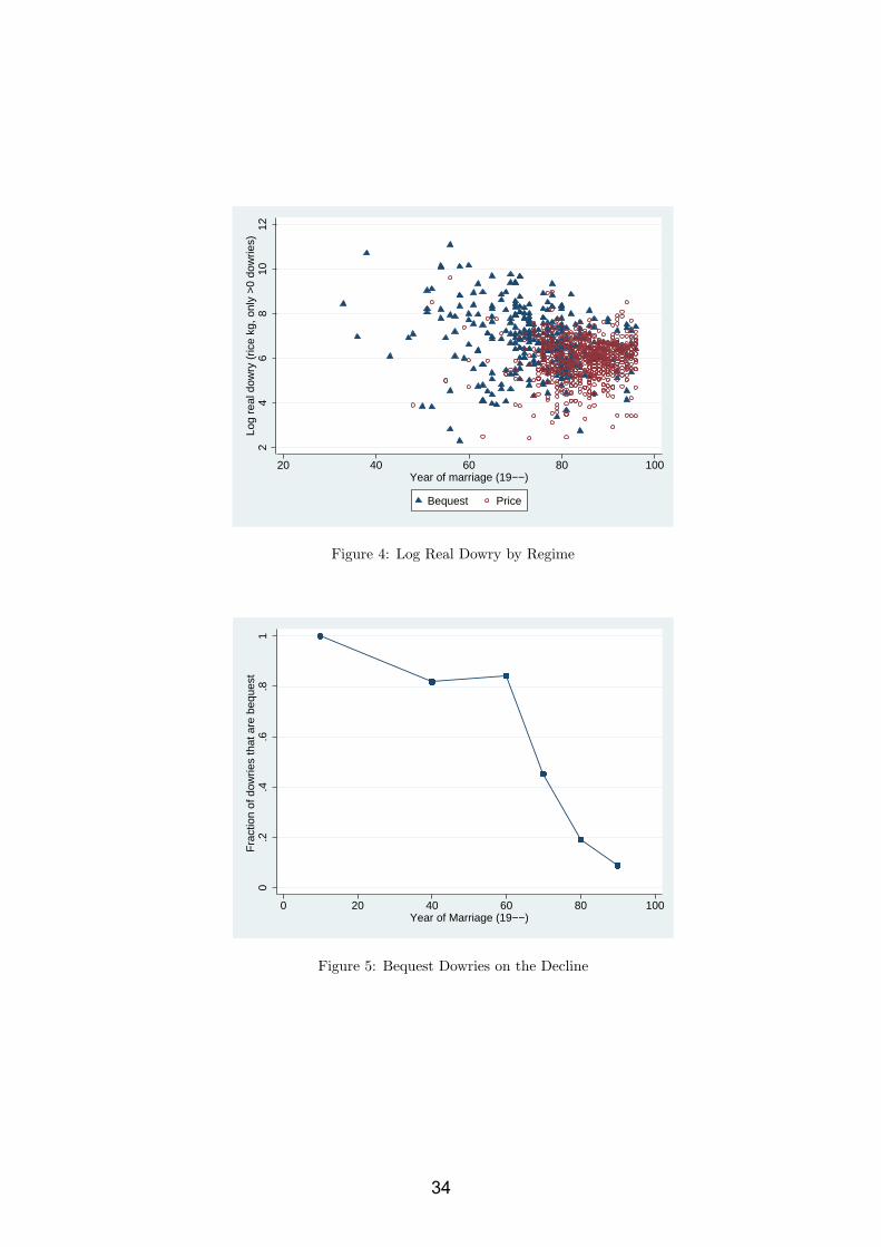
24

68

1012

Log

real

dow

ry (

rice

kg, o

nly

>0

dow

ries)

20 40 60 80 100Year of marriage (19−−)

Bequest Price

Figure 4: Log Real Dowry by Regime

0.2

.4.6

.81

Fra

ctio

n of

dow

ries

that

are

beq

uest

0 20 40 60 80 100Year of Marriage (19−−)

Figure 5: Bequest Dowries on the Decline

34

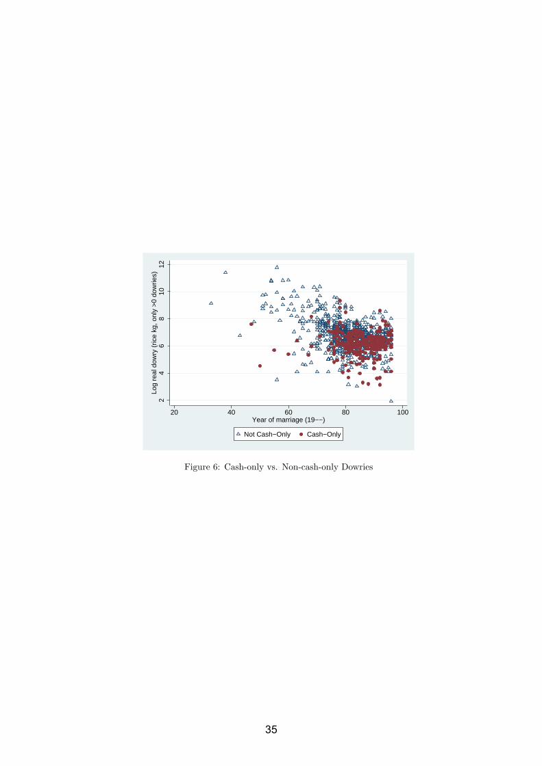
24

68

1012

Log

real

dow

ry (

rice

kg, o

nly

>0

dow

ries)

20 40 60 80 100Year of marriage (19−−)

Not Cash−Only Cash−Only

Figure 6: Cash-only vs. Non-cash-only Dowries

35

Table 1: Some Recent Empirical FindingsFor Price Against Price For Bequest Against Bequest

Rao (1993),Dalmia (2004): India

Edlund (2000): India Edlund (2001): India

Anderson (2004):Urban Pakistan

Anderson (2004):Rural Pakistan

Brown (2003): RuralChinaZhang and Chan (1999):Taiwan

Esteve-Volart (2004):Rural Bangladesh

Esteve-Volart (2004):Rural Bangladesh

Suran et al. (2004):Rural Bangladesh

Botticini (1999):Tuscany 1415-1436

Botticini (1999):Tuscany 1415-1436

36

Table 2: Summary statisticsVariable Mean Std. Dev. N

Year of marriage (19–) 69 16.36 5703Wife’s age 42.3 14.73 5703Wife’s age at marriage 15.3 3.99 5703Husband’s age 47.87 14.23 4181Husband’s age at marriage 24.91 6.47 3758Wife’s BMI 18.71 2.85 5023Wife is underweight 0.51 0.5 5023Wife is normal weight 0.46 0.5 5023Wife is overweight/obese 0.02 0.15 5703Husband’s BMI 18.61 2.44 3502Husband is underweight 0.52 0.5 3502Husband is normal weight 0.46 0.5 3502Husband is overweight/obese 0.01 0.1 5703Wife’s school (years) 1.68 2.71 5616Wife did not attend school 0.62 0.49 5703Wife attended some primary school 0.29 0.45 5703Wife attended some low secondary school 0.07 0.25 5703Wife attended some high secondary school 0.02 0.16 5703Husband’s school (years) 3.22 3.82 3760Husband did not attend school 0.64 0.48 5703Husband attended some primary school 0.2 0.4 5703Husband attended some low secondary school 0.09 0.28 5703Husband some high secondary school 0.07 0.26 5703Hindu 0.1 0.3 5703Love marriage 0.01 0.11 5703Wife’s number of brothers of majority at marriage 1.05 1.26 5703Wife had no brothers of majority at marriage 0.43 0.5 5703Husband’s father was richer than wife’s father 0.38 0.49 5689Wife’s mother’s school (years) 0.61 1.71 5703Wife’s father’s school (years) 2.2 3.48 5703Husband’s mother’s school (years) 0.13 0.77 5703Husband’s father’s school (years) 0.88 2.26 5703Wife’s parents own land 0.25 0.43 5703Wife’s parents’ land value (1996 takas) 58607.66 152758.26 5703Husband’s parents own land 0.37 0.48 5703Husband’s parents’ land value (1996 takas) 81824.98 166599.15 5703Wife was previously married 0.14 0.34 5703Wife’s parents died before her marriage 0.03 0.18 5703Dowry given at marriage 0.3 0.46 5701Nominal dowry (takas) 2451.73 6331.31 5685Real dowry (rice kg) 581.27 4285.52 5685Real dowry (rice kg, only > 0 dowries) 1939.28 7659.17 1704Log real dowry (rice kg, only > 0 dowries) 6.62 1.12 1704

37

Table 3: Pooled and Switching Regression ResultsPooled Switching Price Bequest

(1) (2) (3) (4)Year of marriage (19–) -.022 .045 .045 -.053

(.004)∗∗∗ (.001)∗∗∗ (.005)∗∗∗ (.005)∗∗∗

Wife’s age at marriage -.017 .089 -.034 -.029(.011) (.004)∗∗∗ (.011)∗∗∗ (.014)∗∗

Wife’s BMI .008 .033 .022 .006(.011) (.004)∗∗∗ (.009)∗∗ (.014)

Hindu .767 -.199 .450 1.076(.081)∗∗∗ (.028)∗∗∗ (.075)∗∗∗ (.093)∗∗∗

Wife is literate but did not attend school -.356 -1.072 -.040 -.984(.259) (.090)∗∗∗ (.239) (.203)∗∗∗

Wife attended some primary school .093 .473 .106 .129(.066) (.023)∗∗∗ (.057)∗ (.076)∗

Wife attended some low secondary school .289 .122 .145 .353(.113)∗∗ (.040)∗∗∗ (.092) (.161)∗∗

Wife attended some high secondary school .490 -3.074 1.204 .701(.247)∗∗ (.086)∗∗∗ (.185)∗∗∗ (.188)∗∗∗

Wife’s parents’ land value (1996 takas, ’000s) .001 .000 .000 .001(.000)∗∗ (.000) (.000)∗∗ (.000)∗∗∗

Wife’s mother’s school (years) .021 -.071 -.002 -.003(.018) (.006)∗∗∗ (.022) (.021)

Wife’s father’s school (years) .004 .032 -.013 .035(.010) (.003)∗∗∗ (.008) (.013)∗∗∗

Wife was previously married .192 -.067 .110 .544(.095)∗∗ (.033)∗∗ (.078) (.129)∗∗∗

Wife’s number of brothers of majority at marriage .008 -.040 .035 -.080(.021) (.010)∗∗∗ (.018)∗ (.025)∗∗∗

Husband’s age at marriage -.011 -.013 -.016(.005)∗∗ (.002)∗∗∗ (.004)∗∗∗

Husband’s BMI .022 -.040 .012(.014) (.005)∗∗∗ (.013)

Husband is literate but did not attend school .735 -.963 .900(.289)∗∗ (.100)∗∗∗ (.201)∗∗∗

Husband attended some primary school .227 -.466 .126(.069)∗∗∗ (.024)∗∗∗ (.057)∗∗

Husband attended some low secondary school .275 -.575 .272(.093)∗∗∗ (.032)∗∗∗ (.092)∗∗∗

Husband some high secondary school .699 -1.568 1.008(.118)∗∗∗ (.041)∗∗∗ (.130)∗∗∗

Husband’s parents’ land value (1996 takas, ’000s) .000 .000 .000(.000) (.000)∗∗∗ (.000)

Husband’s mother’s school (years) .025 -.374 -.207(.033) (.011)∗∗∗ (.078)∗∗∗

Husband’s father’s school (years) -.014 -.003 -.010(.012) (.004) (.011)

Husband is polygynous -.538 1.432 -.263(.194)∗∗∗ (.067)∗∗∗ (.192)

Eligible sex ratio (males/females) .711 -1.460 .019(.222)∗∗∗ (.077)∗∗∗ (.272)

Village is electrified .108 -.458 -.004(.059)∗ (.021)∗∗∗ (.054)

Love marriage -1.121(.087)∗∗∗

Husband from same household .931(.041)∗∗∗

Wife’s parents died before her marriage .176(.080)∗∗

Wife had no brothers of majority at marriage .126(.028)∗∗∗

Constant 6.921 -2.671 2.036 10.824(.427)∗∗∗ (.150)∗∗∗ (.470)∗∗∗ (.446)∗∗∗

Obs. 1220 1220 1220 1220Log-likelihood (Pooled) -1690.289Log-likelihood (Mixture) -1559.652R2 .227F statistic 14.049 509.848 20.256 38.363

Note: Dependent variable in columns (1), (3), and (4) is log real dowry in rice kg (sample

mean is 6.165). Dependent variable in column (2) is the probability of being in column (3).

Statistical significance: ∗ 10% ; ∗∗ 5% ; ∗∗∗ 1%. 38

Table 4: Household Characteristics by Predicted RegimeVariable Mean Price Mean Bequest

Real dowry (rice kg, only > 0 dowries) 552.68 2238.93∗∗∗

Cash-only dowry 0.30 0.17∗∗∗

Year of marriage (19–) 84.79 74.73∗∗∗

Wife’s age at marriage 17.27 14.65∗∗∗

Wife’s BMI 18.94 19.06Hindu 0.14 0.23∗∗∗

Wife’s school (years) 1.90 2.46∗∗∗

Wife’s parents’ land value (1996 takas) 53122.9 66310.52Wife’s mother’s school (years) 0.55 1.12∗∗∗

Wife’s father’s school (years) 2.13 3.25∗∗∗

Wife was previously married 0.11 0.11Wife’s number of brothers of majority at marriage 1.25 1.37Husband’s age at marriage 24.62 25.02Husband’s BMI 18.66 18.98∗∗

Husband’s school (years) 2.16 5.64∗∗∗

Husband’s parents’ land value (1996 takas) 86049.96 135329.45∗∗∗

Husband’s mother’s school (years) 0.02 0.59∗∗∗

Husband’s father’s school (years) 1.13 1.85∗∗∗

Husband is polygynous 0.03 0.01∗∗∗

Village is electrified 0.30 0.50∗∗∗

Rooms 2.75 3.12∗∗∗

Love marriage 0.01 0.03∗

Husband from same household 0.07 0.03∗∗∗

Wife’s parents died before her marriage 0.01 0.02Value of all wife’s assets (1996 takas) 40287.32 20290.13Value of wife’s land assets (1996 takas) 24179.53 11453.41Value of all husband’s assets (1996 takas) 80773.38 220820.64∗∗

Value of husband’s land assets (1996 takas) 65789.37 134998.54∗∗∗

Obs. in Predicted Regimes 865 355Note: Statistical significance: ∗ 10% ; ∗∗ 5% ; ∗∗∗ 1%.

39

Table 5: Robustness Check 1: Removing the Non-Membership PredictionsPooled Switching Price Bequest

(1) (2) (3) (4)Year of marriage (19–) -.022 .037 .044 -.059

(.004)∗∗∗ (.001)∗∗∗ (.005)∗∗∗ (.005)∗∗∗

Wife’s age at marriage -.017 .099 -.035 -.020(.011) (.004)∗∗∗ (.011)∗∗∗ (.014)

Wife’s BMI .008 .024 .019 .009(.011) (.004)∗∗∗ (.009)∗∗ (.014)

Hindu .767 -.244 .442 .991(.081)∗∗∗ (.029)∗∗∗ (.075)∗∗∗ (.088)∗∗∗

Wife is literate but did not attend school -.356 -.885 -.239 -.985(.259) (.091)∗∗∗ (.232) (.216)∗∗∗

Wife attended some primary school .093 .246 .091 .059(.066) (.023)∗∗∗ (.057) (.076)

Wife attended some low secondary school .289 -.096 .147 .296(.113)∗∗ (.040)∗∗ (.093) (.154)∗

Wife attended some high secondary school .490 -3.756 1.045 .644(.247)∗∗ (.087)∗∗∗ (.252)∗∗∗ (.192)∗∗∗

Wife’s parents’ land value (1996 takas, ’000s) .0005 -.0001 .0005 .0007(.0002)∗∗ (.00007)∗∗ (.0002)∗∗∗ (.0002)∗∗∗

Wife’s mother’s school (years) .021 -.042 -.002 .001(.018) (.006)∗∗∗ (.022) (.020)

Wife’s father’s school (years) .004 .047 -.011 .042(.010) (.003)∗∗∗ (.008) (.013)∗∗∗

Wife was previously married .192 -.077 .118 .533(.095)∗∗ (.033)∗∗ (.078) (.130)∗∗∗

Wife’s number of brothers of majority at marriage .008 .012 .039 -.038(.021) (.007) (.018)∗∗ (.023)

Husband’s age at marriage -.011 -.013 -.015(.005)∗∗ (.002)∗∗∗ (.004)∗∗∗

Husband’s BMI .022 -.038 .010(.014) (.005)∗∗∗ (.013)

Husband is literate but did not attend school .735 -.643 .871(.289)∗∗ (.102)∗∗∗ (.209)∗∗∗

Husband attended some primary school .227 -.471 .148(.069)∗∗∗ (.024)∗∗∗ (.055)∗∗∗

Husband attended some low secondary school .275 -.628 .255(.093)∗∗∗ (.033)∗∗∗ (.092)∗∗∗

Husband some high secondary school .699 -1.400 .971(.118)∗∗∗ (.041)∗∗∗ (.128)∗∗∗

Husband’s parents’ land value (1996 takas, ’000s) -.0002 .0006 .00006(.0002) (.00006)∗∗∗ (.0002)

Husband’s mother’s school (years) .025 -.364 -.201(.033) (.012)∗∗∗ (.077)∗∗∗

Husband’s father’s school (years) -.014 -.011 -.012(.012) (.004)∗∗∗ (.011)

Husband is polygynous -.538 1.222 -.293(.194)∗∗∗ (.068)∗∗∗ (.193)

Eligible sex ratio (males/females) .711 -1.258 .007(.222)∗∗∗ (.078)∗∗∗ (.271)

Village is electrified .108 -.290 .013(.059)∗ (.021)∗∗∗ (.054)

Love marriage

Husband from same household

Wife’s parents died before her marriage

Wife had no brothers of majority at marriage

Constant 6.921 -2.153 2.257 11.088(.427)∗∗∗ (.150)∗∗∗ (.476)∗∗∗ (.435)∗∗∗

Obs. 1220 1220 1220 1220Log-likelihood (Pooled) -1690.289Log-likelihood (Mixture) -1563.822R2 .227F statistic 14.049 483.223 12.924 38.743Note: Dependent variable in columns (1), (3), and (4) is log real dowry in rice kg (sample

mean is 6.165). Dependent variable in column (2) is the probability of being in column (3).

Statistical significance: ∗ 10% ; ∗∗ 5% ; ∗∗∗ 1%.

40

Table 6: Robustness Check 2: Relaxing the Reduced Form Restrictions

Pooled Switching Bequest Price(1) (2) (3) (4)

Year of marriage (19–) -.022 -.034 .046 -.070(.004)∗∗∗ (.001)∗∗∗ (.006)∗∗∗ (.005)∗∗∗

Wife’s age at marriage -.017 -.116 .007 -.044(.011) (.004)∗∗∗ (.015) (.011)∗∗∗

Wife’s BMI .008 -.019 -.004 .024(.011) (.004)∗∗∗ (.014) (.009)∗∗∗

Hindu .767 .335 .891 .512(.081)∗∗∗ (.028)∗∗∗ (.087)∗∗∗ (.078)∗∗∗

Wife is literate but did not attend school -.356 .003 -1.114 .017(.259) (.089) (.186)∗∗∗ (.266)

Wife attended some primary school .093 -.212 -.055 .091(.066) (.023)∗∗∗ (.079) (.057)

Wife attended some low secondary school .289 -.243 .497 .072(.113)∗∗ (.039)∗∗∗ (.129)∗∗∗ (.102)

Wife attended some high secondary school .490 2.152 .621 -2.299(.247)∗∗ (.086)∗∗∗ (.182)∗∗∗ (.232)∗∗∗

Wife’s parents’ land value (1996 takas, ’000s) .0005 .0001 .0007 .0004(.0002)∗∗ (.00007)∗∗ (.0002)∗∗∗ (.0002)∗∗

Wife’s mother’s school (years) .021 .043 -.014 .020(.018) (.006)∗∗∗ (.019) (.020)

Wife’s father’s school (years) .004 -.017 .039 -.014(.010) (.003)∗∗∗ (.014)∗∗∗ (.009)

Wife was previously married .192 -.126 .721 .124(.095)∗∗ (.033)∗∗∗ (.144)∗∗∗ (.079)

Wife’s number of brothers of majority at marriage .008 -.469 .045 .037(.021) (.010)∗∗∗ (.029) (.019)∗

Husband’s age at marriage -.011 .023 -.027 -.009(.005)∗∗ (.002)∗∗∗ (.005)∗∗∗ (.005)∗

Husband’s BMI .022 .021 .049 .015(.014) (.005)∗∗∗ (.015)∗∗∗ (.013)

Husband is literate but did not attend school .735 .819 .346 .789(.289)∗∗ (.099)∗∗∗ (.254) (.199)∗∗∗

Husband attended some primary school .227 .318 .167 .153(.069)∗∗∗ (.024)∗∗∗ (.088)∗ (.054)∗∗∗

Husband attended some low secondary school .275 .508 .243 .260(.093)∗∗∗ (.032)∗∗∗ (.115)∗∗ (.093)∗∗∗

Husband some high secondary school .699 1.121 .414 .718(.118)∗∗∗ (.041)∗∗∗ (.118)∗∗∗ (.159)∗∗∗

Husband’s parents’ land value (1996 takas, ’000s) -.0002 -.00007 -.0002 .00008(.0002) (.00006) (.0002) (.0002)

Husband’s mother’s school (years) .025 .332 -.025 .009(.033) (.011)∗∗∗ (.029) (.048)

Husband’s father’s school (years) -.014 .054 -.044 -.002(.012) (.004)∗∗∗ (.011)∗∗∗ (.012)

Husband is polygynous -.538 -1.454 .419 -.332(.194)∗∗∗ (.067)∗∗∗ (.328) (.193)∗

Eligible sex ratio (males/females) .711 1.795 .069 -.207(.222)∗∗∗ (.077)∗∗∗ (.235) (.288)

Village is electrified .108 .229 .089 .011(.059)∗ (.021)∗∗∗ (.069) (.054)

Love marriage 1.598(.087)∗∗∗

Husband from same household -.700(.041)∗∗∗

Wife’s parents died before her marriage -.201(.079)∗∗

Wife had no brothers of majority at marriage -.751(.028)∗∗∗

Constant 6.921 2.527 11.268 2.023(.427)∗∗∗ (.149)∗∗∗ (.513)∗∗∗ (.491)∗∗∗

Obs. 1220 1220 1220 1220Log-likelihood (Pooled) -1690.289Log-likelihood (Mixture) -1547.500R2 .227F statistic 14.049 485.459 28.345 18.403

Note: Dependent variable in columns (1), (3), and (4) is log real dowry in rice kg (sample

mean is 6.165). Dependent variable in column (2) is the probability of being in column (3).

Statistical significance: ∗ 10% ; ∗∗ 5% ; ∗∗∗ 1%. 41

Data Appendix

A.1 Matlab Data

The complete dataset is described in Rahman, Menken, Foster, and Gertler (1999).

There are 5312 women for whom year of marriage is reported or can be reconstructed

from age and age at marriage. In addition, we have 391 previous marriages reported,

giving a total of 5703 marriages. Of these, 1731 women report a positive dowry at

the time of marriage. In 562 marriages, the husband confirmed that a dowry was

given, and in 112 marriages, a husband reported a dowry even when the wife did

not.1 This gives a total of 1843 marriages in which dowry was reported. Of these, in

1704 marriages the wife reports the dowry amount (including the value of goods at the

time of marriage). In addition, we have 663 marriages in which the husband reports

the dowry amount but the wife does not. In 556 marriages we have two reports of

dowry; for the results reported, we take the average of the reports.2 All results are

qualitatively similar when we exclude husbands’ dowry reports. Due to other missing

covariates for some marriages, the estimation sample uses 1220 marriages.

Some additional notes on variable construction:

• We use height and weight to calculate Body Mass Index (BMI) and categorize

individuals as underweight, normal weight, or overweight/obese using World

Health Organization guidelines. The vast majority of the sample (97% of women

and 98% of men) have a BMI that is classified as normal or underweight.

• Level of school attainment (primary, low secondary, or high secondary) are as-

signed from the years of schooling, in accordance with Rahman, DaVanzo, and

1In many instances husbands were not interviewed in the survey.2Reported dowry amounts between husband and wife are reasonably correlated; the Pearson

correlation coefficient is 0.62.

42

Razzaque (2003). The omitted category in the regression results is “wife/husband

did not attend school.”

A.2 Rice Prices

No single source contains rice prices for the entire period, so we constructed a se-

ries using the Statistical Abstracts for British India3 for the period 1910-1946; the

Pakistan Central Statistical Office’s Statistical Yearbook 1955 for 1949; the Pakistan

Central Statistical Office’s 20 Years of Pakistan in Statistics for 1950-1967; and the

Statistical Yearbooks of Bangladesh for 1965-1996.4 Duplicate observations for the

years 1964 to 1967 were used to convert between takas and rupees, and overlapping

medium and common rice prices for the years 1950 to 1967 are used to convert between

rice qualities. We used a linear interpolation to cover the missing years (1947-1948).

Real dowries are expressed in (medium quality) rice kilograms.

A.3 Sex Ratio

Constructing a sex ratio time series has proven treacherous in previous dowry work

(Edlund, 2000; Rao, 2000). We adopt a simple approach that takes account of the

mortality trajectory in the years between Census records. We calculate the sex ratio

from the Census Records of India (1931, 1941), Pakistan (1951, 1961), and Bangladesh

(1974, 1984). Where possible, we use the lowest level of geographic detail to corre-

spond with the district in the Matlab study, although this was not possible for early

years of the Census records, particularly the Indian Census records. Taking the count

of males and females in the Census year, we construct the adjusted sex ratio as de-

3Volumes compiled before partition but published afterward are simply called Statistical Abstract,India.

4Details of the sources as well as unit conversions are given in Table A.

43

scribed by Rao (1993), where the adjusted sex ratio gives the number of males aged

20-29 divided by the number of females aged 10-19. We calculate the relevant ratio

for each age group, from ages 10 to age 90, using the same ten year differential.

For the years between the Census years, the cohorts’ age and mortality, particu-

larly child mortality in the earlier years of our records, is pronounced, so the relevant

sex ratio for each age must be adjusted for mortality each year. We use the actual

number of males and females in the Census year, and then use the period lifetable

constructed with the Census records to derive an estimate of survivorship to the next

age (nqx). Since these values will differ for both men and women, the sex ratio will

change for the years between Censuses. For example, males aged 20-29 in 1961 will be

aged 25-34 in 1966, and the best available estimate for the fraction of men surviving

to that age would be the period survival rate for men aged 25-34 in 1961. For the

final Census we use, we create a quasi-synthetic cohort and assume that the course

of mortality over the subsequent years will be the same as for the later cohorts whose

mortality trajectory is recorded in the Census.

Appendix References

Edlund, L. (2000): “The Marriage Squeeze Interpretation of Dowry Inflation: Com-ment,” Journal of Political Economy, 108(6), 1327–1333.

Rahman, M., J. DaVanzo, and A. Razzaque (2003): “When Will BangladeshReach Replacement-level Fertility? The Role of Education and Family PlanningServices,” Working Paper.

Rahman, O., J. Menken, A. Foster, and P. Gertler (1999): “The MatlabHealth and Socioeconomic Survey: Overview and User’s Guide,” DRU-2018/1,RAND, Santa Monica, CA.

Rao, V. (1993): “The Rising Price of Husbands: A Hedonic Analysis of DowryIncreases in Rural India,” Journal of Political Economy, 101(4), 666–677.

(2000): “The Marriage Squeeze Interpretation of Dowry Inflation: Re-sponse,” Journal of Political Economy, 108(6), 1334–1335.

44

Table A: Rice Price Sources

Years covered Source Details

1910-1929 Statistical Abstract for British India 1931 No. 300, pg. 671 [Variations in Average AnnualRetail Prices Current of Food Grains in BritishIndia]. Common rice in Dacca, rupees per maund(base year: 1873= 100 rupees).

1912-1932 Statistical Abstract for British India 1934 No. 301, pgs. 764-765 [Average Annual RetailPrices Current of Food Grains in British India].Common rice in Dacca, rupees per maund.

1930-1939 Statistical Abstract for British India 1941 No. 164, pg. 445 [Average Annual Retail PricesCurrent of Food Grains in British India].Common rice in Dacca, rupees per maund.

1942-1946 Statistical Abstract, India 1949 No. 165, pg. 1238 [Average Annual Retail PricesCurrent of Food Grains in British India].Common rice in Dacca, rupees per maund.

1949 Statistical Yearbook 1955,Pakistan Central Statistical Office

No. 67, pg. 105 [Average (Annual) Retail Pricesof Important Articles Consumed by the IndustrialWorkers at Dacca]. Medium rice, rupees per seer.

1950-1967 20 Years of Pakistan in Statistics,Pakistan Central Statistical Office

Table 11.7 [Average Retail Prices of BasicArticles of Consumption in East Pakistan].Common and medium rice in Dacca, rupees perseer.

1965-1967 Statistical Yearbook of Bangladesh 1975 Table 8.1 [Annual Average Retail Price ofSelected Consumer Goods in Dacca, pg. 195].Medium rice, takas per maund.

1968-1978 Statistical Yearbook of Bangladesh 1979 Table 10.6 [Annual Average Retail Price ofSelected Consumer Goods in Dhaka, pg. 374].Medium rice, takas per maund.

1978-1988 Statistical Yearbook of Bangladesh 1989 Table 10.16 [Annual Average Retail Price ofSelected Consumer Goods in Dhaka, pg. 448].Medium rice, takas per seer.

1987-1996 Statistical Yearbook of Bangladesh 1997 Table 10.16 [Annual Average Retail Price ofSelected Consumer Goods in Dhaka, pg. 477].Medium rice, takas per kilogram.

Unit conversions (2000 Statistical Yearbook of Bangladesh, pgs. 645-650):1 kilogram = 1.071 seer = .0267 maund.

45