on the experimental determination of damping of metals and...
TRANSCRIPT

On the Experimental Determination of Damping of Metals and Calculation of Thermal Stresses in
Solidifying Shells


On the Experimental Determination of Damping of Metals and Calculation of Thermal Stresses in
Solidifying Shells
Jonas Åberg
Doctoral Thesis
Materials Processing Department of Material Science and Engineering
School of Industrial Engineering and Management Royal Institute of Technology SE-10044 Stockholm, Sweden
Akademisk avhandling som med tillstånd av Kungliga Tekniska Högskolan i Stockholm framlägges till offentlig granskning för avläggande av teknologie doktorsexamen, torsdag den
15 juni 2006, kl. 10.15, Sal M3, Brinellvägen 68, KTH, Stockholm.
TRITA-MG 2006-03, ISSN-1104-7127, ISBN 91-7178-377-6
Jonas Åberg, On the Experimental Determination of Damping of Metals and Calculation of Thermal Stresses in Solidifying Shells
School of Industrial Engineering and Management
Department of Materials Science and Technology, Materials Processing
Royal Institute of Technology
SE-100 44 Stockholm, Sweden
TRITA-MG 2006-03
ISSN-1104-7127
ISBN 91-7178-377-6
© Jonas Åberg, juni 2006

v
On the Experimental Determination of Damping of Metals and Calculation of Thermal Stresses in Solidifying Shells Jonas Åberg 2006 Department of Materials Science, Royal Institute of Technology S-100 44 Stockholm, Sweden
Abstract This thesis explores experimentally and theoretically two different aspects of the properties
and behaviour of metals: their ability to damp noise and their susceptibility to crack when solidifying.
The first part concerns intrinsic material damping, and is motivated by increased demands from society for reductions in noise emissions. It is a material’s inherent ability to reduce its vibration level, and hence noise emission, and transform its kinetic energy into a temperature increase. To design new materials with increased intrinsic material damping, we need to be able to measure it. In this thesis, different methods for measurement of the intrinsic damping have been considered: one using Fourier analysis has been experimentally evaluated, and another using a specimen in uniaxial tension to measure the phase-lag between stress and strain has been improved. Finally, after discarding these methods, a new method has been developed. The new method measures the damping properties during compression using differential calorimetry. A specimen is subjected to a cyclic uniaxial stress to give a prescribed energy input. The difference in temperature between a specimen under stress and a non-stressed reference sample is measured. The experiments are performed in an insulated vacuum container to reduce convective losses. The rate of temperature change, together with the energy input, is used as a measure of the intrinsic material damping in the specimen. The results show a difference in intrinsic material damping, and the way in which it is influenced by the internal structure is discussed.
The second part of the thesis examines hot cracks in solidifying shells. Most metals have a brittle region starting in the two-phase temperature range during solidification and for some alloys this region extends as far as hundreds of degrees below the solidus temperature. To calculate the risk of hot cracking, one needs, besides knowledge of the solidifying material’s ability to withstand stress, knowledge of the casting process to be able to calculate the thermal history of the solidification, and from this calculate the stress. In this work, experimental methods to measure and evaluate the energy transfer from the solidifying melt have been developed. The evaluated data has been used as a boundary condition to numerically calculate the solidification process and the evolving stress in the solidifying shell. A solidification model has been implemented using a fixed-domain methodology in a commercial finite element code, Comsol Multiphysics. A new solidification model using an arbitrary Lagrange Eulerian (ALE) formulation has also been implemented to solve the solidification problem for pure metals. This new model explicitly tracks the movement of the liquid/solid interface and is much more effective than the first model.
Descriptors: material damping, measurement methods, calorimetric methods, optical strain gauge measurements, hot cracking, stress in solid shells, ALE

vi

vii
”Intet är som väntanstider…” Fridolins visor, Erik Axel Karlfeldt
"We have a habit in writing articles published in scientific journals to make the work as finished as possible, to cover up all tracks, to not worry about the blind alleys or describe how you had the wrong idea first...So there isn't any place to publish, in a dignified manner, what
you actually did in order to get to do the work."
Richard Feynman, Nobel Lecture 1966

viii
ix
Supplements The thesis includes the following supplements
Supplement 1
Investigation of the Damping in Twelve Metallic Plates Using Frequency Response Jonas Åberg, Björn Widell, Petra Larsson Submitted for publication to Experimental Techniques ISRN KTH-MG-INR-06:04 SE TRITA-MG 2006:04
Supplement 2
Uniaxial material damping measurements using a fiber optic lattice: a discussion of its performance envelope Jonas Åberg, Björn Widell Experimental Mechanics, v 44, n 1, February 2004, p 33-36
Supplement 3
Measurement of intrinsic material damping using differential calorimetry on specimens under uniaxial tension Jonas Åberg, Björn Widell, Thomas Bergström and Hasse Fredriksson Thermochimica Acta, Volume 411, Issue 2, 5 March 2004, Pages 125-131
Supplement 4
Intrinsic Material Damping in Mg, Al and Fe Alloys and a Discussion of its Dependence on the Internal Structure of the Material Jonas Åberg, Björn Widell, Hasse Fredriksson ISRN KTH-MG-INR-06:05 SE TRITA-MG 2006:05
Supplement 5
An On-Site Experimental Heat Flux Study and its Interpretation in a Femlab Finite Element Simulation of Continuous Casting of Copper in The South-Wire Process Jonas Åberg, Michael Vynnycky, Hasse Fredriksson Trans. Indian Inst. Met., vol.58, 2005, pp. 509-515.
Supplement 6
Development of a finite element model for study of the developing stress and strain in a solidifying shell Jonas Åberg, Michael Vynnycky, Hasse Fredriksson ISRN KTH-MG-INR-06:06 SE TRITA-MG 2006:06
Supplement 7
Modelling of Thermal Stresses in Industrial Continuous Casting Processes Jonas Åberg, Michael Vynnycky, Hasse Fredriksson Proceedings of the Femlab Conference, Stockholm, Sweden 2-4 October 2005

x

xi
Contents ABSTRACT .................................................................................................................... V SUPPLEMENTS.......................................................................................................... IX CONTENTS ................................................................................................................ XI 1 INTRODUCTION................................................................................................. 1 2 DAMPING IN METALS .......................................................................................4 2.1 INTRODUCTION............................................................................................................. 4 2.2 EXPERIMENTAL METHODS ............................................................................................ 5 2.2.1 Method 1, Supplement 1.................................................................................................. 5 2.2.2 Results ......................................................................................................................... 7 2.2.3 Discussion..................................................................................................................... 7 2.2.4 Method 2, Supplement 2.................................................................................................. 8 2.2.5 Results ....................................................................................................................... 10 2.2.6 Discussion................................................................................................................... 11 2.2.7 Method 3, Supplement 3 and 4 ....................................................................................... 11 2.2.8 Results ....................................................................................................................... 16 2.2.8.1 Thermoelasticity ...................................................................................................................16 2.2.8.2 Intrinsic damping measurements ...........................................................................................17 2.3 DISCUSSION OF DAMPING MEASUREMENTS ................................................................. 19 3 HOT CRACKS IN SOLIDIFYING SHELLS ...................................................... 21 3.1 INTRODUCTION........................................................................................................... 21 3.2 MATERIAL BEHAVIOUR................................................................................................ 21 3.3 IN SITU INDUSTRIAL MEASUREMENTS .......................................................................... 25 3.3.1 Process description......................................................................................................... 25 3.3.2 Experimental methods................................................................................................... 26 3.3.2.1 Evaluation of measured data .................................................................................................26 3.3.2.2 Simulation solidification models ............................................................................................27 3.3.3 Results ....................................................................................................................... 27 3.3.4 Discussion................................................................................................................... 29 3.4 SIMULATION MODEL 1, SUPPLEMENT 6 ........................................................................ 30 3.4.1 Method....................................................................................................................... 30 3.4.2 Results, Solidification and stress simulation........................................................................ 31 3.5 SIMULATION MODEL 2, SUPPLEMENT 7 ........................................................................ 33 3.5.1 Solidification method for pure metals ................................................................................. 33 3.5.2 Results ....................................................................................................................... 34 3.6 DISCUSSION................................................................................................................. 34 4 THESIS CONCLUSIONS ................................................................................... 35 5 FUTURE WORK.................................................................................................. 36 6 ACKNOWLEDGEMENTS.................................................................................. 37 7 REFERENCES .................................................................................................... 38

xii

1
1 Introduction The thesis you are about to read consist of work in two different areas, damping and hot
crack formation. The two areas might seem totally disparate at first glance but when put into perspective it turns out that although this was not intentional when the work started, it has some connecting points.
When trying to control a material manufacturing process there is a multitude of data and relations to consider to ascertain the highest possible production rate and quality. With a material manufacturing process in this text, it is primarily the production of bulk material that is considered, but the thoughts are general and can be applied to the manufacturing of components as well.
The most fundamental thing to always keep in mind is that the manufacturing process is like an anchor chain – it depends on all the links. The weakest link in a manufacturing process is the step causing the unwanted property – and cannot be fixed by the process steps later in the manufacturing chain. The property can be things like formation of inclusions causing premature failure in rotation machinery, to high oxygen content causing brittleness in copper, to high hydrogen content in the melt during solidification or many other problems. If these problems are not taken care of not to appear they can most often not be fixed later in the production.
In Figure 1 a small tree of boxes are drawn trying to describe how we can work on finding a method to control a process. We will discuss it in the context of avoiding hot cracks. Later we will discuss the appearance of hot cracks in more detail.
During solidification, after the solid shell can start to accept some load but above a certain temperature, most metals are brittle [1, 2]. By this we mean that the material will fracture in a brittle way as opposed to ductile. In a brittle fracture the material does not deform plasticly before it breaks.
The idea is to understand how certain properties appears and can be controlled in manufacturing casting processes. This includes but is not confined to the appearance of hot cracks.
Hot cracks are caused by a combination of low strength and low ductility in a material at elevated temperatures and applied tensile stress. In a cast material the tensile stress can be developed thermally as well as mechanically. Materials are often brittle at high temperatures and undergo a transition to a ductile behaviour at a specific temperature called the ductile-brittle transition temperature, TDB, or the zero ductility temperature, ZDT. The ductile-brittle transition temperature is found below the coherence temperature, were the coherence temperature, Tc, defines the temperature were the material can accept a mechanical load. For a material with a dendritic solidification this temperature is above the solidus temperature of the material. Above the ductile-brittle transition temperature the material is very sensitive for hot tearing when tensile stress is applied.
The proneness to hot cracking is an important property. All metals at one stage have to pass through this temperature range. Fortunately nature has provided us with a number of materials were this is not a practical problem so we have been able to produce a multitude of alloys based on different basic elements such as iron, copper and aluminium. However, as we design new materials with improved properties some of the new materials are much harder to produce and process due to these alloys higher susceptibility to hot cracks. In some cases the

2
new materials can not be produced efficiently at all and sometimes with low productivity. The same problem exists for alloys of all three of the big base alloys, iron copper and aluminium.
A description of the areas that need investigation to be able to tackle the whole chain of events that triggers the non-wished for appearance of hot-cracks can be understood by viewing Figure 1.
The property the algorithm describes is hot cracks but might suite as a general algorithm of how to investigate and build up know-how about how to avoid or achieve a specific property. The concept of a property in Figure 1 has to be read in a wide context. A property can for example be interpreted as the answer to the question “will a hot crack appear?”
Figure 1, How to foresee hot cracks in a process
Below, the letters refer to the letters within brackets in Figure 1. The leftmost branch regards the materials behaviour and how to understand and explain it.
(A) Why is it that some materials are so much more sensitive to cracking at elevated temperatures? This can be that a material for certain alloy compositions during certain solidification conditions (e.g. temperature and solidification speed) undergoes a solid phase transition. This solid phase phase-transition means a momentary change of density which in turn might create cracks.
(B) To investigate this and understand it we have to be able to measure the property. In this case, we need to measure how sensitive the metal is to cracking by making experimental tensile tests at different temperatures below the coherence temperature in the material.
We get to the second, middle branch in Figure 1.
(C) After making the experiments we can form models about why the material behaves the way it does, but also form descriptive models of the material behaviour.
This far, if we allow us to believe in the method of Figure 1, we have understood the material behaviour by making experiments, and we have formed models of the behaviour. The

3
next step is to understand how the process work, and how the process relates to the modelled property.
The rightmost branch of Figure 1 describes the modelling and calculation of data to make it possible to compare with the model of the property to see whether it will appear or not. In the case studied we want to know whether a hot crack will appear or not.
To do this we need to know the tensile stress levels the solidifying melt will experience during solidification and cooling. To do so in this case, we need to know how and at what rate energy is transported away from the melt, and subsequently, from the solid shell. There exists no good theoretical model that is practically possible to use to model the heat transfer from the liquid to the mould in an industrial process. Therefore, we need to measure how the heat is transported away from the melt to the surrounding to use as boundary conditions for the subsequent calculations. We believe it is easier and more realistic to measure rather than to model this very complicated process. However – if this modelling problem is solved it is easy to implement it into this scheme.
(E) We also need to have a model of the solidification to use for our calculations. When we have measured the heat transfer and formed models of it to use in our calculations we can calculate the temperature verses time for the melt and solid (F) and use these data to calculate the evolving stress in the solid shell.
(G) When we have calculated the stress we can compare it to the model of the material property, that is check the stress, temperature derivative and temperature and compare it with the model in (C) and make a prediction whether we will get a crack or not (H).
To make these calculations a number of data about the materials and process is needed which all need to be experimentally determined.
In the presented work the other common denominator for the two parts is the experimental work. In the first part regarding damping a method was developed to study a metals intrinsic material damping to be able to understand how it depends on the internal structure of the material. This could be seen as work in the box marked (B) in Figure 1. The idea is to in the future make models to predict the damping for materials to be able to take this parameter into consideration when designing new materials.
In the second part of the thesis regarding hot crack formation no known methods to measure the heat transfer from a moving mould in an industrial process to use as boundary conditions for numerical simulation of solidification and stress build up in a solidifying shell is known to the authors. In this work a method to measure this energy transfer has been developed. Referring once more to Figure 1, this would correspond to work in box D.

4
2 Damping in metals
2.1 Introduction During the last forty years there has been a continuous strive to reduce sound emissions.
Increased demands from the public and ever steadily increasing requirements from environmental authorities have led to national, European community and international regulations regarding sound emissions.
The industrial revolution has brought a steady development of products. From the start in the early 19th century until today millions of products have been produced reflecting the needs of society. Functionality was the first requirement sought after, later when seeking to expand the market new design requirements such as form, colour, ease of use, safety and many others have appeared.
During the post-war era, the development of vehicles capable of ever-higher speeds, both on ground, at sea and in air has emphasised the need for designs that decrease the sound emissions. Both internal emissions and external is of importance. People like to work and travel in a quiet environment. The truck driver needs a low noise workplace to be able to stay alert at the wheel, the same goes for the aircraft crew as well as the passengers that want to arrive at the destination well rested for the working day or the vacation ahead. The external noise levels are of equal importance. Few people want to live near highly trafficked streets due to the noise levels, and this goes to an even higher extent for living areas around airports.
During the recent decades, noise emissions have been increasingly seen as an environmental issue. Consumers and authorities have both put new demands on the environment [3]. Consumers have regarded low noise levels as a competitive advantage when choosing a car, a way of transportation, electric home appliances such as videocassette recorders. Authorities have put increasing demands and enforced legislation in the field of decreasing the level of noise in all parts of society. Examples are the federal aviation regulations (FAR) [4] and joint aviation requirements (JAR) [5] putting demands on sound emission from aircraft at take off and landing, the European economic community’s demands on sound emissions from the heavy truck industry [6], machinery in general [7] as well as Swedish legislation restricting the maximum allowed noise level in living quarters and during work [8].
Product manufacturers have addressed these demands in different ways. Some have tried to encapsulate the noise-emitting source, some have tried to add sound absorbing materials to the design and others have designed the components as to reduce the sound emission from the product.
Examples of the first kind, encapsulation is to put the sound source in a closed room with walls covered in vibration absorbing material. The second is to clad the vibrating sound emitting source in a high damping material. The third is to make designs without or with few thin sections that otherwise would transfer the vibration energy into the surrounding air, and to use joints within the design that absorbs energy.
Other examples when the methods above are insufficient are passive or active dampers. It has been tried to analyse the frequency and amplitude of the structure and mount small blocks containing a spring, mass and damper system on it. The block is designed to act as a damper for the structure it is mounted on. A second, active method is to continuously measure the

5
frequency spectra near the ear of the person disturbed by the noise, analyse it, produce sound in opposite phase and play it through loudspeakers close to the ear to counteract the noise.
All the above methods take a toll in price, complexity, weight, appearance or functionality. To avoid the above, there are circumventing methods, the first is to design products that do not generate sound and vibration at all. If this is not possible damping can be addressed at the design and development stage of the material. It would therefore be highly desirable to address the problem of damping at an early stage of the design process, the design and production of the material itself.
To be able to meet the demands on materials that fulfil traditional specifications as well as having good damping properties it is necessary to take the material damping property into consideration when designing new materials.
The material damping should be a parameter among others during the product design process. The same way as other material properties such as Young’s modulus, creep curves, yield stress, hardness, density and thermal properties such as thermal conductivity and thermal capacity is tabulated in tables, the damping should be stated.
In order to take the property material damping into consideration when designing new materials, there is a need to know how the internal structure of materials affect it. One has to build models of the damping behaviour, and to build these models there is a need to measure the material damping as a function of the material structure, both on a micro and macro scale.
2.2 Experimental methods In this work several ways to measure damping were considered. The first conclusion was to
regard damping as an intrinsic property of a material. The property sought for was the internal inherent property damping in a material, not the damping due to the shape of the specimen, or the damping due to friction in the joint between the specimen and the adjoining structure, neither damping due to acoustic emissions to the surrounding media.
2.2.1 Method 1, Supplement 1 The realisation came as a result of the work described in supplement 1. The reason for the
method used was plain and simple that a number of material samples were at hand to be tested on. The idea of the test method can be understood by studying Figure 2. A linear system depicted by the box in the picture is fed with a known or measurable input signal 1( )v t [9]. The system will change the input signal in such a way that the output signal from the system is
2 ( )v t . The way the system affects the input signal can be described by a function ( )ωH j .
1( )v t 2 ( )v t1( )G jω 2 ( )G jω( )H jω
Figure 2, Frequency response concept

6
Using this description of the system we can after transforming the input signal write the behaviour of the system as an equation.
ω ω ω=2 1( ) ( ) ( )G j H j G j (1.1)
I turns out that if we take the Fourier transform of the input signal, 1( )v t , and the output signal, 2 ( )v t , ( )ωH j can be calculated as the quotient of the two. The function ( )ωH j , usually called the frequency response function (FRF) is then analysed and a value of the damping can be evaluated.
The input signal is created by hitting the test sample with an impulse hammer with a force transducer in the tip, Figure 3. The output is measured by placing an accelerometer somewhere on the test sample. The calculation of the frequency response function is automatically done by the test equipment used while the evaluation of the damping was done in a computer program written by the authors.
Figure 3, Experimental setup
The neat idea with the method in supplement one is that the analysis is simple in theory. One plots the amplitude spectrum of the frequency response function, finds a peak indicating a resonance, checks the coherence for a validation of the experimental data and then plots the data around the resonance in an argand plane. The position of the circle and the angle pointing out the resonance can be used to interpret the loss factor, Figure 4.
Figure 4, The circle fit method
7
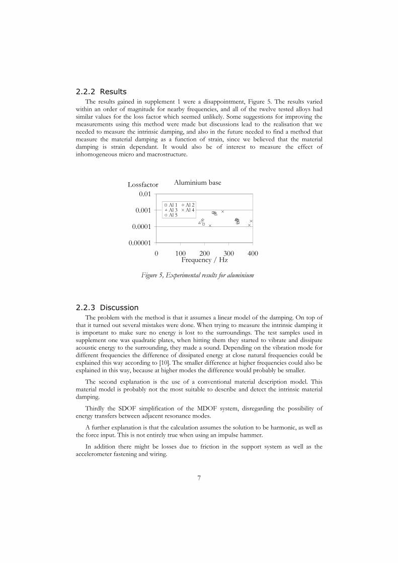
2.2.2 Results The results gained in supplement 1 were a disappointment, Figure 5. The results varied
within an order of magnitude for nearby frequencies, and all of the twelve tested alloys had similar values for the loss factor which seemed unlikely. Some suggestions for improving the measurements using this method were made but discussions lead to the realisation that we needed to measure the intrinsic damping, and also in the future needed to find a method that measure the material damping as a function of strain, since we believed that the material damping is strain dependant. It would also be of interest to measure the effect of inhomogeneous micro and macrostructure.
Aluminium base
0.00001
0.0001
0.001
0.01
0 100 200 300 400Frequency / Hz
Al 1 Al 2Al 3 Al 4Al 5
Lossfactor
Figure 5, Experimental results for aluminium
2.2.3 Discussion The problem with the method is that it assumes a linear model of the damping. On top of
that it turned out several mistakes were done. When trying to measure the intrinsic damping it is important to make sure no energy is lost to the surroundings. The test samples used in supplement one was quadratic plates, when hitting them they started to vibrate and dissipate acoustic energy to the surrounding, they made a sound. Depending on the vibration mode for different frequencies the difference of dissipated energy at close natural frequencies could be explained this way according to [10]. The smaller difference at higher frequencies could also be explained in this way, because at higher modes the difference would probably be smaller.
The second explanation is the use of a conventional material description model. This material model is probably not the most suitable to describe and detect the intrinsic material damping.
Thirdly the SDOF simplification of the MDOF system, disregarding the possibility of energy transfers between adjacent resonance modes.
A further explanation is that the calculation assumes the solution to be harmonic, as well as the force input. This is not entirely true when using an impulse hammer.
In addition there might be losses due to friction in the support system as well as the accelerometer fastening and wiring.
8
An intrinsic limitation of this method is that it cannot detect damping as a function of strain, as the strain is different in different parts of the plate during its bending.
To improve this method and for future work we suggest to use a rod rather than a plate to lessen the loss into acoustic energy and to do the testing in a vacuum chamber.
When the damping is independent of strain, amplitude it is said to be linear [22]. If the damping is linear, the measured value will equal the intrinsic damping as shown in equation (1.2)
1measured l l
V
dVV
η η η= =∫ (1.2)
where measuredη is the measured volume average loss factor, lη is the intrinsic linear loss
factor and V is the volume of the specimen. On the other hand, if the damping is dependent on the strain amplitude, equation (1.3), it is easy to see that ( )measuredη η ε≠
1( ( ))measured
V
x dVV
η η ε= ∫ (1.3)
where ( )η ε is the loss factor as a function of the strain, ε , and x is a vector defining a infinitesimal volume element.
It is easy to appreciate that this makes it impossible to measure the intrinsic material damping unless we know for a fact that the damping is linear or if we use a method that introduces a non-homogeneous strain into the specimen.
2.2.4 Method 2, Supplement 2 A number of methods were considered. One group of methods is based on the damping of
torsional vibration, with or without continuous force input in air or vacuum [11, 12, 13]. It was discarded due to varying strain in different parts of the twisting rod. Different types of pendulums such as found in [14]. Another group is based on the decay of bending beams, also with or without continuous force input [15, 16]. Or other systems based on springs [17] or signal analysis methods [18].Some commercially available systems have also been considered, e.g. the Differential Mechanical Analyser marketed by Netzsch, [19], or the dynamic characterisation test suite supplied by MTS, [20], but they either does not use uniaxial stress or only work for high damping materials.
The decision fell on a development of an experimental setup proposed and evaluated by Kinra et al to measure the damping in uniaxial tension. In a number of articles [21, 22, 23, 24] Kinra et al describes a method to measure damping using the relationship between stress and strain as a function of time. It can be used to determine the damping as the phase difference between the time-harmonic waves representing the load and the corresponding strain. When a periodic excitation is applied, the strain will lag behind the stress. The corresponding phase lag is a direct measurement of the damping in the specimen. Kinra et al found that it is possible to directly measure the phase difference in the time domain for big phase differences between stress and strain. For materials with low damping such as metals, however, where the phase difference is in the order of 10-4 rad, it is virtually impossible to detect this small phase difference in the time domain. They found, however, that in certain cases it is possible to

9
measure the phase angle of the fast Fourier transforms (FFT) of the stress and strain signals individually. The FFT of each signal was calculated and the phase component corresponding to the excitation frequency was recorded. The phase angles were subtracted to give a corresponding value for the phase difference and consequently, the material damping.
In their experiments, they used a tensile test machine with conventional strain gauges for stress and strain, strain-bridge amplifiers, instrument amplifiers and a digital oscilloscope.
One problem with this technique is that great care has to be taken to avoid any reactive components to induce phase shift between the specimen and the finally calculated FFT. This includes all components such as the digital oscilloscope, the instrument amplifier, the strain bridges and the strain gauges themselves. All phase shifting equipment had to be redesigned using better components that do not cause phase shifting. After doing this, Kinra et al reports the accuracy in measuring the phase shift between two sinusoidal waveforms to be 9.59*10-5 radians.
Kinra et al described their problems in avoiding the pitfalls of the phase shift design of the electronic components in their system. Since this seemed troublesome I wanted to use the basic idea to measure the phase shift between stress and strain, but use a non-electric method to avoid electric disturbances in the system. The decision was to use light, since it is well known to be insensitive to electric influence. As reported in [25], it is indeed possible to measure strain using light.
The basic idea is to inscribe an optical fibre Bragg grating along the optic fibre. When transmitting light through the fibre, the wavelength corresponding to the fringe pattern is reflected or transmitted, depending on the design of the fringes; the fringe pattern works as a filter. Let us have a look at Figure 6. If we choose the wavelength of the source, λ, to be close to the characteristic wavelength of the fringe pattern, λ1, we will get a certain reflected or transmitted intensity of light, I1. If we then keep the source wavelength constant λ, represented by the straight vertical line, and strain the fibre, the length between the fringes will increase, and hence its characteristic wavelength λ2. The corresponding intensity I2, together with the original strain level I1, will together with the characteristics of the curve give the change in strain
Wavelength
Intensity
I1
I2
λ1λ2
λ
Figure 6, The principle of an optical strain gauge

10
As is described in some detail in supplement two, a new instrument setup was designed to feed the optical fibres with laser light of a known adjustable wave length, and then feed the response from the optical strain gauges to an apparatus that could directly read the difference in time when the signal reached the centre of the bar.
2.2.5 Results Before funds were invested in some very expensive equipment a fundamental flaw in the
basic design was realized.
To be able to measure the phase lag between stress and strain, it must be possible to measure the stress or at least assume that stress is present before the strain is measured. Kinra et al solved this problem by putting a strain gauge at the beginning and in the middle of the bar. The strain gauge at the beginning was there to indicate the stress, assuming that stress is present along the entire bar more or less instantaneously. The second strain gauge in the middle was there to indicate when the strain appears.
The fundamental problem is that the wave propagation velocity in metals is far from infinite, i.e. typically 5000 meters per second for iron based alloys. Kinra et al claims their
method works down to phase differences of π= -5
16
29.587*10
2, a value based on the phase
resolution of their 16 bit processor oscilloscope. This is most probably an overestimation of the sensitivity of the method.
The stress must reach the strain signal sensor well before the strain sensor gives a reading. The time it takes for the stress wave to propagate will be calculated and then the phase lag will be converted into a time lag, and compared to find the limitations of the method.
The time it takes for the elastic wave from the stress sensor to reach the strain sensor depends on the speed of sound, the wave propagation speed, in the material. Lets call the length between the two sensors l and the speed of sound in the material a. The time it takes for the sound wave to propagate will be
soundlta
= (1.4)
The time equivalent for a certain phase lag, Φ , can be calculated by comparing with the frequency, f, with which the load is applied.
{ } arctan( )tan( )
2 2equivtf f
ηη
π πΦ
= = = Φ = (1.5)
The criterion for success is to make sure that sound equivt t< which gives us the following expression.
η ηπ π
< ⇒ <arctan( ) arctan( )
2 2l l aa f f
(1.6)

11
Different figures for the longitudinal wave propagation velocity exist in the literature, but most metals like iron, magnesium and aluminum alloys have a speed of sound between 5800 and 6400 m/s [26, 27].
As an example it is shown that the derived relation proves that for a loss factor of 10-3 measured at 1 Hz, the sensors should be less than 1 m apart. In the same way, at 10 Hz, less than 0.1 meter apart and at 100 Hz, less than 0.01 meter apart. If the loss factor is an order of magnitude smaller, as can be expected for low damping metals, the situation gets worse by an order of magnitude and the sensors have to be mounted unreasonably close to each other. This calculation is based on the assumption that it is enough if the stress wave arrives first, but that would give inaccurate results, since we would not be able to see the difference in the lag due to the speed of sound and the internal diffusion of energy in the material. It will probably be necessary to get a margin between the time it takes the stress wave to reach the centre and the time it takes for the strain wave to reach it.
2.2.6 Discussion The conclusion of the work leading to the second work presented in this thesis is; the
practical problems of mounting the stress and strain sensors very close to each other make it impossible to use the method unless the damping in the material is high, and the frequency is low.
The method would be excellent if it was possible to somehow measure the stress independently. The authors know of no such method. Another possibility would be to measure the speed of sound in the material independently of the lag between the stress and strain and compensate for the time lag caused by the speed of sound. This seems not possible due to the various speed of sound values reported for various types of transmission of sound in solid materials [26] and [27].
2.2.7 Method 3, Supplement 3 and 4 The method use a basic assumption, according to thermodynamics, that the internal losses
in the material are transformed to other forms of energy, and that this energy can be measured as a temperature increase in the material.
The idea is elemental in its simplicity. A cyclic load is imposed on a bar. The mechanical energy input into the system is carefully measured. The temperature raise of the bar is measured. The internal damping is then essentially the energy corresponding to the temperature increase divided by the mechanical energy input.
One needs to take care of some problems. Heat might escape the bar via its ends. Friction of the ends might work as an energy source input. One needs to measure the load and temperature carefully.

12
Figure 7, Principal set-up
Convection losses are held to a minimum using a vacuum chamber for the experiments. The radiation losses are small due to the small temperature difference, but may be made even smaller by using reflecting surfaces in the future. Conduction loss and gain via the ends is the major concern, but tests indicate that results can be ascertained before the disturbance propagates to the sensors in the middle of the rod, as is shown in supplement 3.
Tests have been carried out showing the temperature increase to be measurable and reproducible.
The relation between the input of energy and heating is then a measure of the damping in the material. Initial calculations were performed to estimate the heating rate as a function of the input of mechanical energy. The basic idea is to impose the load during uniaxial testing. It is evenly distributed within the material without plastic deformation and all energy from damping is converted to heat and measured as a temperature increase. This temperature increase depends on the density, volume and specific heat of the material. It was also assumed that the loss of energy to the surroundings is negligible. The calculations indicate that it should be possible to measure the temperature increase due to the intrinsic internal damping if it is possible to ascertain that only small amounts of energy transfer takes place between the test piece and the surroundings.
Two bars are placed in a vacuum chamber. The test bar is in contact with the top and bottom of the vacuum chamber whilst the reference bar is suspended from a plastic hook in the ceiling, insuring that it does not touch the measured bar or the walls of the test chamber. The temperature of the test bar as a function of time is measured differentially to the reference bar using thermocouples. The vacuum chamber is placed inside an MTS [28] tensile test machine with compression platens. The test bar will thus be cyclically stressed by compression. Two control and measurement systems are used, one to control and measure the load input, the other to measure the temperature increase.
13
Sub-systems: Figure 7 illustrates the general sub-system assembly. It consists of a load-input system in the form of a tensile test machine, a vacuum system to reduce convective heat transfer and a differential temperature measurement system consisting of two bars, thermocouples and a microvolt meter.
Load input system: The system used to impose the compression load on the test bar is a conventional tensile test machine.
Cu
Cu/
Ni
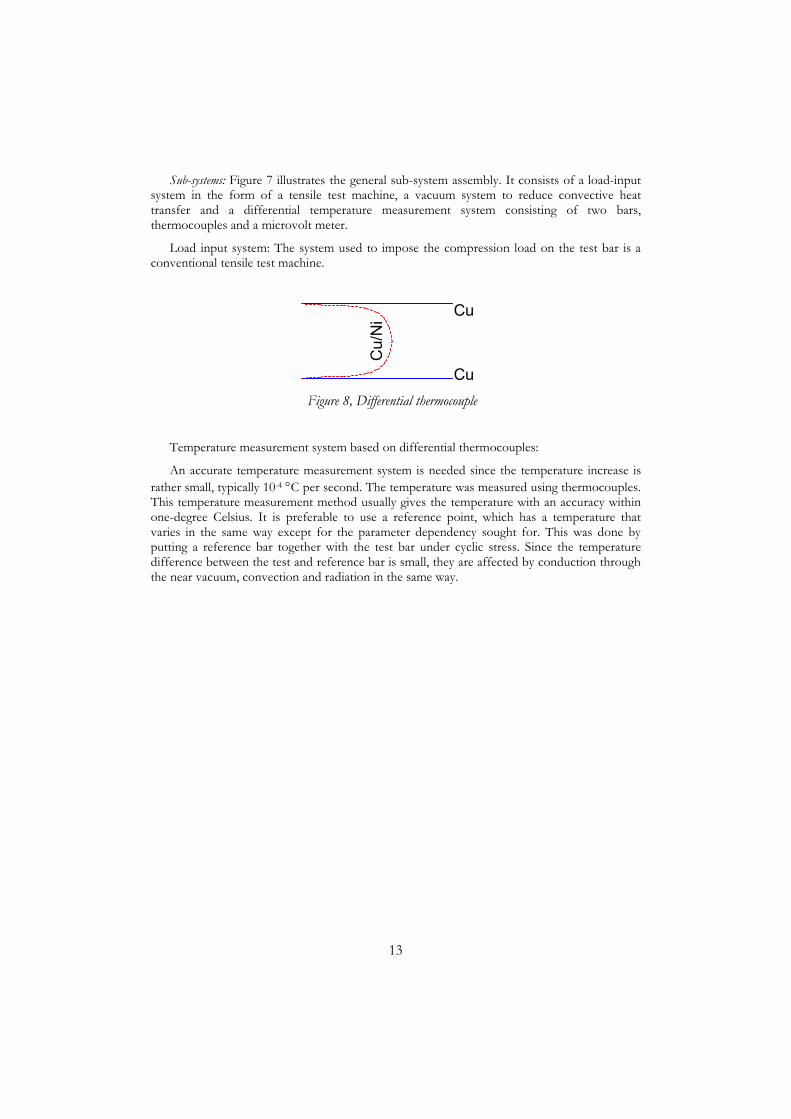
Cu Figure 8, Differential thermocouple
Temperature measurement system based on differential thermocouples:
An accurate temperature measurement system is needed since the temperature increase is rather small, typically 10-4 °C per second. The temperature was measured using thermocouples. This temperature measurement method usually gives the temperature with an accuracy within one-degree Celsius. It is preferable to use a reference point, which has a temperature that varies in the same way except for the parameter dependency sought for. This was done by putting a reference bar together with the test bar under cyclic stress. Since the temperature difference between the test and reference bar is small, they are affected by conduction through the near vacuum, convection and radiation in the same way.

14
Figure 9, The test bars and vacuum chamber
Type-T thermocouples, copper/constantan, with a Seebeck coefficient of about 40.3 μV/°C at 20°C were used [29].The two wires were separated. The blue Cu wires leads from the measurement instrument into the vacuum chamber. The tips of the two blue wires were inter-connected using a red Cu/Ni wire, each connection being a sensor. One was placed on the test bar, the other on the reference bar, Figure 8.
Figure 9 shows the mounting. The thermocouple wires, the cardboard and the paperclip can be seen. It is also possible to observe a hole in the upper part of the shorter reference bar, which is used to hang the bar in. The design of the hole and the hook means that the bar is unable to twist and minimises the risk for contact with the measurement bar or the walls of the vacuum chamber.
The test chamber is a tube with connectors to the vacuum system for the extraction of air, a dummy that is not used and a connector for all the thermocouples, Figure 9. To minimise external electric interference's all the thermocouples were protected with a coaxial shield with common electric ground to the rest of the measurement system.
During initial testing, it was discovered that the MTS machine caused considerable thermal disturbance. After the initial period of time during which the test and reference bar were meant to come to thermal equilibrium, there was still an approximately linear temperature variation in the bar, a few degrees higher at the lower end than at the higher end. At the start of the experiment, the lower end of the bar was heated more than the upper end. This was due to the
15
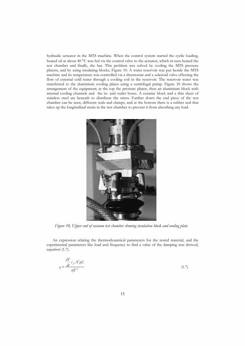
hydraulic actuator in the MTS machine. When the control system started the cyclic loading, heated oil at about 40 °C was fed via the control valve to the actuator, which in turn heated the test chamber and finally, the bar. This problem was solved by cooling the MTS pressure platens, and by using insulating blocks, Figure 10. A water reservoir was put beside the MTS machine and its temperature was controlled via a thermostat and a solenoid valve effecting the flow of external cold water through a cooling coil in the reservoir. The reservoir water was transferred to the aluminium cooling plates using a centrifugal pump. Figure 10 shows the arrangement of the equipment; at the top the pressure platen, then an aluminium block with internal cooling channels and the in- and outlet hoses. A ceramic block and a thin sheet of stainless steel are beneath to distribute the stress. Further down the end piece of the test chamber can be seen, different seals and clamps, and at the bottom there is a rubber seal that takes up the longitudinal strain in the test chamber to prevent it from absorbing any load.
Figure 10, Upper end of vacuum test chamber showing insulation block and cooling plate.
An expression relating the thermodynamical parameters for the tested material, and the experimental parameters like load and frequency to find a value of the damping was derived, equation (1.7).
2p
2
dT c A ρEdtη =πfF
(1.7)

16
Were, dTdt
is the temperature gradient during the test just after applying the cyclic load, pc
is the specific heat at constant pressure, A is the cross sectional area of the bar, ρ the density, E Youngs modulus, f the frequency and F the force used.
From the beginning it was feared that disturbances from the end of the bars would interfere with the measurements. It was thought that friction between the end of the bars and the endplates could produce heat that together with outside temperature changes could result in temperature gradients that propagate through the bar during the experiment. This would give an additional temperature increase, which could be misinterpreted as an increase in the intrinsic damping in the bar.
2.2.8 Results To make a conservative estimate of the time it takes for an external disturbance to
propagate from the end to the sensor in the middle of the test bar, the following method was used. The temperature of the cooling water of the cooling plates was raised by about 20 degrees. The temperature versus time curves for the differential sensors were recorded. It was concluded that it takes about five minutes before this external disturbance reaches the middle and affects the reading for an aluminium alloy, Figure 11. This is a conservative estimate since the external heat source is considerably smaller during an experiment. For steels and cast iron, the undisturbed time is longer due to the lower diffusion rate of heat in these materials. The step function temperature in Figure 11 is scaled down by a factor of 50.
0 500 1000−0.1
0
0.1
0.2
0.3
0.4
0.5
Time / s
T /
K
Water scaled by 50
Thermocouplesat ends
Thermocouple at center of bar
Figure 11, Experimental temperature distribution
Some results from the damping related experiments performed in supplement 3 and 4.
2.2.8.1 Thermoelasticity It was interesting to find that the thermoelastic effect was clearly visible. A instantaneous
load increase results in a instantaneous temperature increase, Figure 12. The temperature

17
amplitude during load shifts was shown to agree reasonably well with classical theory on thermoelasticity, Figure 13.
-0.02
0.00
0.02
0.04
0.06
0 100 200 300 400 500time /s
T / K
Figure 12, The experimental value of an aluminium alloy exposed to a square wave load.
0.E+00
1.E-09
2.E-09
3.E-09
4.E-09
5.E-09
1 4 7 8 13Alloy number
dT/d
p /
K/Δσ
Experiment ΔT/ΔσTheory dT/dp=T*β/(ρ*Cp)
Figure 13, The thermoelastic effect for different materials presented in supplement 4.
2.2.8.2 Intrinsic damping measurements A typical output of a test and its evaluation can be seen in Figure 14 and Figure 15. At first
the system is at rest and the temperature at both ends of the bar and the centre are at the same level. Then at a prescribed time a sinusoidal load is applied, and the losses in the rod make the temperature increase. The ends of the bar will rise in temperature differently compared to the centre since it is in closer contact with the surrounding. It could either be chilled by the surrounding cooling system or be heated by friction between the end of the bar and the end plates. Regardless of the type of disturbance, the important thing is that this disturbance does not interfere with the measured value in the centre of the bar during the duration of the test.

18
Figure 14, Grey Cast Iron, SS0120, sand cast, 35Hz, 0.4-15.4 kN, Temperature - time plot.
0 100 200 300 400 500 600 700-0.5
0
0.5
1
1.5
2
Time / s
Tem
pera
ture
diff
eren
ce /
K
Exponential Temp-Time derivative 0.0029866 K/s 95% Confidence intervalon dTdt 0.88%
Compensated dTdt 0.0029737 K/s
Figure 15, Exponential fit for the grey cast iron in Figure 14 with an error estimate.
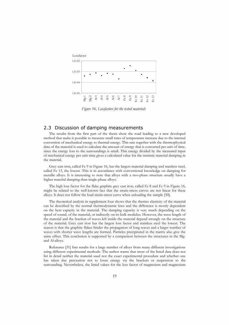
If there is an overall change in temperature, for example a slow rise or decline in the room temperature, then there will be a temperature gradient observable in the graphs prior to the start of the experiment. This gradient is compensated for as shown in Figure 15 where there is a value for the compensated temperature gradient. In Figure 16 a couple of measured and evaluated lossfactors can be observed for some tested alloys.
19
1.E-05
1.E-04
1.E-03
1.E-02
Mg
1
Mg
2
Al 3
Al 4
Al 5
Al 6
Al 7
Fe 8
Fe 9
Fe 1
0
Fe 1
1
Fe 1
2
Fe 1
3
Lossfactor
Figure 16, Lossfactors for the tested materials
2.3 Discussion of damping measurements The results from the first part of the thesis show the road leading to a new developed
method that make it possible to measure small rates of temperature increase due to the internal conversion of mechanical energy to thermal energy. This rate together with the thermophysical data of the material is used to calculate the amount of energy that is converted per unit of time, since the energy loss to the surroundings is small. This energy divided by the measured input of mechanical energy per unit time gives a calculated value for the intrinsic material damping in the material.
Grey cast iron, called Fe 9 in Figure 16, has the largest material damping and stainless steel, called Fe 13, the lowest. This is in accordance with conventional knowledge on damping for metallic alloys. It is interesting to note that alloys with a two-phase structure usually have a higher material damping than single-phase alloys.
The high loss factor for the flake graphite grey cast iron, called Fe 8 and Fe 9 in Figure 16, might be related to the well-known fact that the strain-stress curves are not linear for these alloys. It does not follow the load strain-stress curve when unloading the sample [30].
The theoretical analysis in supplement four shows that the thermo elasticity of the material can be described by the normal thermodynamic laws and the difference is mostly dependent on the heat capacity in the material. The damping capacity is very much depending on the speed of sound, of the material, or indirectly on its bulk modulus. However, the wave length of the material and the fraction of waves left inside the material depend strongly on the structure of the material. Grey cast iron has the largest loss factor and stainless steel the lowest. The reason is that the graphite flakes hinder the propagation of long waves and a larger number of waves with shorter wave lengths are formed. Particles precipitated in the matrix also give the same effect. This conclusion is supported by a comparison between the structures in the Mg- and Al-alloys.
Reference [31] lists results for a large number of alloys from many different investigations using different experimental methods. The author warns that most of the listed data does not list in detail neither the material used nor the exact experimental procedure and whether one has taken due precaution not to loose energy via the brackets or suspension to the surrounding. Nevertheless, the listed values for the loss factor of magnesium and magnesium

20
alloys is in the range from 6*10-6 – 9*10-1, for aluminium and its alloys 1*10-5 – 2*10-1 and for iron base metals between 6*10-7 – 8*10-2. These literature data indicates a huge span for each base element group. This large span in reported loss factor can be seen to reflect both a large dependence on material structure of the tested materials due to differences in alloying, internal structure and indirectly on the manufacture and process parameters. It can also be seen to reflect the different accuracy of the different methods used in the damping measurements leading to the reported values.
Our measurements give values within the reported span, measured with what we consider to be good accuracy. Developing the method further would give even better accuracy and possibility to extend the test parameter envelop.

21
3 Hot cracks in solidifying shells
3.1 Introduction Of key interest is the heat transfer that occurs during solidification, since this is thought to
be responsible for the appearance of surface and half-way cracks within the solidified shell [32, 33, 34, 35, 36]. As a result, a number of attempts have been to compute the levels of thermally induced stresses and strains that develop in the solidifying shell. These works either simplify the problem to one dimension [37], 38, 39] or develop specially-designed geometry-dependent code to solve the structural equilibrium equations to obtain the thermally-induced stresses and strains in the shell [40, 41, 47, 48].
The first of the three last supplements is about the development of a measurement system to measure the energy transfer from the solidifying melt to the moving mould in an industrial process. The data is then used as boundary condition for solidification calculations.
The measurement of boundary conditions relates to D in Figure 1. Since no method exists to accurately predict the heat transfer from the solidifying shell to the surroundings it is necessary to measure it. In the process studied here, the South Wire process, this can be done since the strand is, as we will see, in time wise contact with a mould during the solidification. It is possible to calculate the energy transfer from the shell by measuring the temperature gradient through the mould and by using Fourier’s law of cooling.
The last two papers are about calculating the solidification sufficiently accurate to use as input data for stress calculations in a solidifying shell. A first attempt was used to use existing solidification models using a source term for the latent heat but it was found to be numerically difficult, supplement 6. Instead a new solidification model was used using a moving mesh solution were the mesh boundary movement between the solid shell and the liquid interiors is modelled by a Stefan condition [42].
3.2 Material behaviour It has been described in literature that most metals are brittle at very high temperatures.
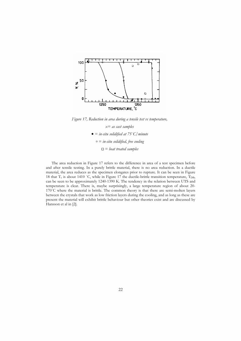
This has been described and discussed by [2, 43, 44, 45]. In general, the material behaviour is as shown in Figure 17 and Figure 18 taken from [1], which are for a carbon steel with a composition of 0.51%C, 0.2%Si, 0.62%Mn, 0.02%P and 0.019%Sn. Figure 17 shows the ultimate tensile stress (UTS) a specimen can take up, prior to rupture, as a function of temperature. In general, the temperature at which the material can take up any load at all, the coherence temperature Tc, is at or above the solidus temperature but lower than the liquidus temperature of the material. For temperatures lower than Tc, the ultimate tensile stress increases as the temperature decreases.
22
Figure 17, Reduction in area during a tensile test vs temperature,
x= as cast samples
•= in-situ solidified at 75˚C/minute
= in-situ solidified, free cooling
= heat treated samples
The area reduction in Figure 17 refers to the difference in area of a test specimen before and after tensile testing. In a purely brittle material, there is no area reduction. In a ductile material, the area reduces as the specimen elongates prior to rupture. It can be seen in Figure 18 that Tc is about 1410 ˚C, while in Figure 17 the ductile-brittle transition temperature, TDB, can be seen to be approximately 1240-1390 K. The tendency in the relation between UTS and temperature is clear. There is, maybe surprisingly, a large temperature region of about 20-170˚C where the material is brittle. The common theory is that there are semi-molten layers between the crystals that work as low friction layers during the cooling, and as long as these are present the material will exhibit brittle behaviour but other theories exist and are discussed by Hansson et al in [2].

23
Figure 18, Ultimate tensile stress vs. temperature
x= as cast samples
•= in-situ solidified at 75˚C/minute
= in-situ solidified, free cooling
= heat treated samples
How these considerations are used can be described by looking at Figure 19, which shows the schematic temperature distribution for a pure single-phase material undergoing one-dimensional solidification. It indicates that the part of the solidified shell with temperature greater than TDB will experience brittle fracture if it is stressed over the ultimate tensile stress. In similar fashion Figure 20 from [46] show two cases in the upper right part of the figure. The curves show the stress as a function of the distance from the mould wall for two different solidification cases. The top point for each curve represents the stress for a certain point experiencing a specific temperature. If one checks in the graph to the upper left, it is possible to see if the stress--temperature value will be above or below the UTS curve. If it is above the curve two cases are possible which can be checked by looking in the bottom left graph. If the temperature is below TDB, the material will deform plastically; if above TDB, it will fracture.

24
T
Cooling water (or mould)
Melt
TDB
Solidificationfront
T 0
Solid shell
TmeltTcoherence
Ductile/brittletransition
Figure 19, A one dimensional view on the crack sensitive region
This material description, the authors believe, makes it possible to use a linear material description model. If we were interested in the behaviour at lower temperatures, we would need to expand the treatment with a material description that handles creep, but in this high temperature range it is not needed.
solid liquid
Stress
xTTc
TDB T
Figure 20, Principle sketch, two cases one leading two a crack, the other not
25
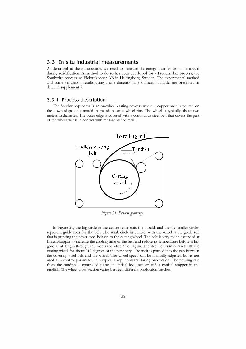
3.3 In situ industrial measurements As described in the introduction, we need to measure the energy transfer from the mould during solidification. A method to do so has been developed for a Properzi like process, the Southwire process, at Elektrokoppar AB in Helsingborg, Sweden. The experimental method and some simulation results using a one dimensional solidification model are presented in detail in supplement 5.
3.3.1 Process description The Southwire-process is an on-wheel casting process where a copper melt is poured on
the down slope of a mould in the shape of a wheel rim. The wheel is typically about two meters in diameter. The outer edge is covered with a continuous steel belt that covers the part of the wheel that is in contact with melt-solidified melt.
Figure 21, Process geometry
In Figure 21, the big circle in the centre represents the mould, and the six smaller circles represent guide rolls for the belt. The small circle in contact with the wheel is the guide roll that is pressing the cover steel belt on to the casting wheel. The belt is very much extended at Elektrokoppar to increase the cooling time of the belt and reduce its temperature before it has gone a full length through and meets the wheel/melt again. The steel belt is in contact with the casting wheel for about 210 degrees of the periphery. The melt is poured into the gap between the covering steel belt and the wheel. The wheel speed can be manually adjusted but is not used as a control parameter. It is typically kept constant during production. The pouring rate from the tundish is controlled using an optical level sensor and a conical stopper in the tundish. The wheel cross section varies between different production batches.
26
3.3.2 Experimental methods
3.3.2.1 Evaluation of measured data The temperature was measured on-site using a number of thermocouples placed in the
casting wheel. A number of industrial measurement campaigns have been performed, each with its own setup, but in principal the following method has been used.
The aim with the measurements has been to evaluate the heat transfer from the hot inner side to the water cooled outside of the mould. To do this we need to use Fourier’s law,
Tq kx∂
=∂
, where q is the energy transfer rate per unit area, k is the coefficient of thermal
conduction, T is temperature and x is the coordinate direction from the hot to the cold side.
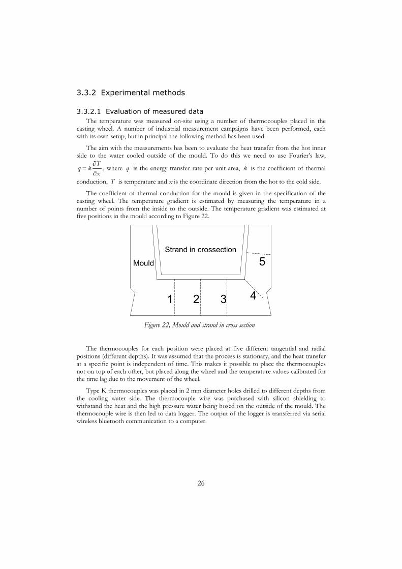
The coefficient of thermal conduction for the mould is given in the specification of the casting wheel. The temperature gradient is estimated by measuring the temperature in a number of points from the inside to the outside. The temperature gradient was estimated at five positions in the mould according to Figure 22.
1 2 3 4
5Strand in crossection
Mould
Figure 22, Mould and strand in cross section
The thermocouples for each position were placed at five different tangential and radial positions (different depths). It was assumed that the process is stationary, and the heat transfer at a specific point is independent of time. This makes it possible to place the thermocouples not on top of each other, but placed along the wheel and the temperature values calibrated for the time lag due to the movement of the wheel.
Type K thermocouples was placed in 2 mm diameter holes drilled to different depths from the cooling water side. The thermocouple wire was purchased with silicon shielding to withstand the heat and the high pressure water being hosed on the outside of the mould. The thermocouple wire is then led to data logger. The output of the logger is transferred via serial wireless bluetooth communication to a computer.
27
3.3.2.2 Simulation solidification models A model was developed to simulate the solidification of pure metals in the finite element
method computer program Femlab. The one dimensional version of the model was verified against an analytical solution to trim the model parameters for optimal accuracy.
A two dimensional version of the model was used with the experimentally evaluated data for the energy transfer rate as a function of time.
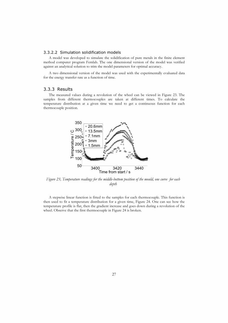
3.3.3 Results The measured values during a revolution of the wheel can be viewed in Figure 23. The
samples from different thermocouples are taken at different times. To calculate the temperature distribution at a given time we need to get a continuous function for each thermocouple position.
3400 3420 344050
100
150
200
250
300
350
Time from start / s
Tem
pera
ture
/ C
20.6mm13.5mm7.1mm3mm1.5mm
Figure 23, Temperature readings for the middle-bottom position of the mould, one curve for each
depth
A stepwise linear function is fitted to the samples for each thermocouple. This function is then used to fit a temperature distribution for a given time, Figure 24. One can see how the temperature profile is flat, then the gradient increase and goes down during a revolution of the wheel. Observe that the first thermocouple in Figure 24 is broken.

28
0 0.005 0.01 0.015 0.02 0.025
100
150
200
250
300
350
Distance from interface
Tem
pera
ture
/ C
03691215182124273033
Figure 24, Temperature profiles for the middle-bottom position during one revolution. Each curve
represents the number of seconds since the melt hit the mould wall indicated by the labels.
It is also of interest to view the three dimensional representation of the heat transport away from the melt, Figure 25.
Figure 25, Surface temperature gradients.
The time axis represents one revolution of the wheel, about 40 seconds. The melt/mould coordinate is the dimensionless distance from the bottom middle of the mould, via the corner up to half the height of the side of the mould. dT/dx indicates the temperature gradient from the hot melt, and is indirectly an indication of the energy transfer rate through the mould, and thus, from the solid shell. Before analysing the result we should note that the completely

29
solidified shell leaves the mould at about 25s, after that the plot is insignificant as it does not give any information about the energy transfer from the strand anymore.
s
Figure 26, The melt/mould coordinate used in Figure 25 is labelled s.
3.3.4 Discussion The interesting thing to note – which has earlier just been suspected – is that the
measurements indicate that the strand when solidifying creates an air gap and then reattaches back and forth. This is indicated by the wavy surface of the graph in Figure 25. The changing heat transfer will create hot and cold spots on the strand which in turn qualitatively indicates the existence of varying thermal stresses on the strand due to the successive cooling, reheating and cooling of the strand surface. These hot and cold spots can sometimes be visible by ocular inspection during casting of the strand as it leaves the casting wheel.
In the results of supplement 5, there is also a comparison with using only one measurement position in the bottom of the mould and the data represented in Figure 25 as boundary condition for a solidification simulation of the process. It turns out that when we only use the bottom measured position we over estimate the energy transfer away from the mould. The reason for this is that we generally have lower heat transfer from the corner, were an air gap is formed early and has lower energy transfer than the flat bottom during the whole solidification process. The results indicate that a surface measurement method of the heat transfer is important to get an accurate understanding of the heat transfer and subsequently, to get accurate solidification simulation results.

30
3.4 Simulation model 1, supplement 6
3.4.1 Method As described in the previous section it was possible to get sufficiently accurate temperature
curves by first comparing with the exact analytical Stefan-solution for a system of a semi-infinite mould and a semi-infinite melt. However, it turns out that this is not good enough for the stress calculations.
The problem is that the classical stress relations used in solid strength mechanics, the Navier equations, are derived for a body with a known reference state. With this is meant that there exists a temperature were the body is stress free. This is described in a thesis [47] and articles[48].
In our case, for a solidifying body, such a state does not exist. In the melt we have a truly shear stress free state but as soon as a solid shell is formed, it will accept loads, and as the temperature sinks the shell will shrink and cause thermal loads. If these thermal loads are tensile, and if the solid shell closer to the melt is in the region were it is brittle and the load is higher than the ultimate tensile stress of the material the material will experience a brittle fracture – a hot crack.
It so turns out, that for linear materials, the Navier equations for a solidifying shell looks exactly the same, just that all the terms are derivatives with respect to time.
This means that we can solve the same solidification problem, use the same numerical methods developed for stationary bodies with a stress free reference state to calculate the parameters in the Navier equation, only that they are not what they seem, instead they are the time derivatives of the same equation.
By taking the results and integrating them for each point in the shell starting from the time the particular point solidified until the time of interest we can get the wanted for parameter.
The algorithm to follow is shown in Figure 27. First we calculate the solidification to get the temperature as a function of time. We then calculate the stress. Unfortunately as mentioned earlier, the structural mechanic calculation subsystem in commercial applications are not adopted for solidification problems. Also, in the software we are using, Comsol Multiphysics, only a plane strain model is easily available. We therefore need to expand the plane strain calculation to a general plane strain model by the assumption that the strain derivative in the out of plane direction is a linear function, as defined in Figure 27. We then get an extra variable to solve for and therefore need an extra equation. We used the integral constraint given in the same figure. The details can be found in supplement 6 and 7.
The problem with the solidification simulation is then that the time derivated version of the Navier equation contains the temperature derivative, and we need the time derivative to be able to integrate it later to get the solution for stress and other problem parameters.
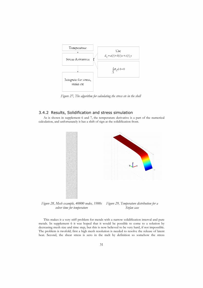
31
( ) ( ) ( )z a t b t x c t yε = + +
0zA
dAσ =∫
Figure 27, The algorithm for calculating the stress etc in the shell
3.4.2 Results, Solidification and stress simulation As is shown in supplement 6 and 7, the temperature derivative is a part of the numerical
calculation, and unfortunately it has a shift of sign at the solidification front.
Figure 28, Mesh example, 40000 nodes, 3300s solver time for temperature
Figure 29, Temperature distribution for a Stefan case
This makes it a very stiff problem for metals with a narrow solidification interval and pure metals. In supplement 6 it was hoped that it would be possible to come to a solution by decreasing mesh size and time step, but this is now believed to be very hard, if not impossible. The problem is twofold; first a high mesh resolution is needed to resolve the release of latent heat. Second, the shear stress is zero in the melt by definition so somehow the stress

32
calculation needs to be turned of in the melt. This is hard to do in a numerically accurate fashion.
As can be seen in Figure 28 were a very dense mesh is used, forcing the time step down in the numerical solution. This particular example has a simulation time of about 3300 s, but no substantial improvements is gained when increasing the number of nodes and subsequently, the solver time to several days. Figure 29 shows the temperature distribution, and the temperature looks qualitatively fine, as is expected from many earlier reported results and also when compared to an analytical solution.
Figure 30, Temperature derivative, cooling wall to the right
Figure 31, Stress, cooling wall to the right
The problem arrives when we get to the temperature derivative. It has a sign shift at the solidification front as can be proved analytically. Sign shifts in gradients are hard to resolve numerically as is clearly shown in Figure 30. The jagged appearance of the graph would not be as evident in a one dimensional graph but is clearly seen here in a two dimensional plot. Since the temperature gradient is integrated this numerical disturbance is multiplied over the whole solidification history and in Figure 31 it is evident that the final result, in this case the stress is far from the correct solution.

33
3.5 Simulation model 2, supplement 7
3.5.1 Solidification method for pure metals Instead of pursuing this line of development a new method has been developed using ALE
– arbitrary Lagrangian Eulerian formulation were the interface between the solid shell and the melt is used in a balance equation were the speed of the solidification front is included. This derived speed is then used to describe the movement of the mesh used in the solution.
s l cs f
s l melt
T T dyk k Hy y dt
T T T
ρ∂ ∂− = Δ∂ ∂= =
s moldT T=
l castT T=0lT
x∂ =∂
( )cy y t=
0sTx
∂ =∂
0, 0xyu τ= = ( ) , 0z xyu t xε τ= =
0, 0xyv τ= =
0, 0y xyσ τ= =
Figure 32, Mesh for ALE case, 250 nodes, 20 s solution time for temperature with the interface between solid and liquid visible
Figure 33, Energy balance at solid liquid interface
The heat balance in Figure 33 is used to model the movement of the solid liquid interface. The details of this new method are described in supplement 7.

34
Figure 34, Agreement between analytical and numerical results
3.5.2 Results The approach using a moving mesh solution gives an exceptional improvement in accuracy
and solving time. The example in Figure 32 with result for the temperature gradient in Figure 34 use 250 nodes and a solver time of 20 s. This is an improvement of more than 160 times in solver time and probably several thousand times when comparing with comparable accuracy.
The second advantage is that we totally separate the liquid and solid domains in the solution, so we do not need to handle the zero strain condition in the melt, we just solve for the stress and strain in the solidified shell.
The agreement between an exact analytical solution and the numerical result for the temperature derivative can be seen in Figure 34. In general, the agreement between simulations and analytical solutions are very good. Further results are presented in supplement 7.
3.6 Discussion To be able to predict whether a material will crack or not due to build-up of thermal
stresses in the shell during solidification one needs, in short hand notation, material data, boundary conditions and a way to calculate the solidification and the stress out of these.
The first part regarding material characterisation and why the material behaves the way it does have been researched by others. The later three of these is addressed in this thesis. A method has been developed to measure the energy transfer to be used as boundary condition, but also to understand the behaviour of the process in a qualitative way.
A conventional solidification model has been found to be usable for temperature calculations during solidification, but not accurate enough for stress calculation. Therefore a better and much faster and more accurate method has been developed using a moving mesh solution for the interface between the solid and liquid.
The ground is thus prepared to feed data from the measurements into the solidification and stress model to calculate the stress.

35
4 Thesis conclusions A number of methods have been considered for measurement of the intrinsic material
damping of metals. Two of these methods have been analysed in detail and experiments evaluated for one of the methods before discarding them, as described in supplement 1 and 2.
A new method based on differential thermal analysis (DTA) during cyclic loading has been developed. The experiments conducted with this method have shown that it is possible to measure the small temperature increase rate due to the internal dissipation of energy. This rate, together with the thermophysical data of the material and the cyclic load data makes it possible to calculate the material damping of the specimen as described in supplement 3.
A number of materials have been tested and the results are discussed in supplement 4.
A method has been developed to measure temperature in a moving mould using wireless transferring of measurement of data and recalculating these for use as a Neumann type boundary condition for solidification simulations.
An existing solidification model has been evaluated by comparing with analytical solutions and found to give reasonable results for temperature but inferior quality for the temperature derivative. This is unacceptable for stress, strain and displacement calculations and the predicted success in future development to solve this seems small for pure metals and alloys with very narrow solidification interval.
Instead, a new solidification and stress calculation model has been developed and checked against analytical solutions with excellent agreement for both temperature, temperature gradient stress and strain when compared to an analytical solution. This new model uses a moving mesh solution for the solidification front and except the very good accuracy; this new model is also much faster.
36
5 Future work Regarding the first part of the thesis regarding damping measurements it would be very
interesting to rebuild the equipment to use uniaxial tension rather than compression. This would make it possible to use thin rods and make it possible to vastly increase the load without risking buckling in compression. The higher load would increase measurement accuracy further as well as make it easier to run frequency and amplitude parameter studies.
It would also be interesting to test anisotropic materials with parameter studies of load and frequency dependence. The purpose of this is would be to build a database relating material parameters to damping for many alloys to find the fundamental relation between material damping and other material parameters.
In the second part regarding hot cracks and stress in solidifying shells it would be interesting to continue the work by replacing the present Stefan case with real measured boundary conditions measured as in supplement 5. Further it would be interesting to expand the ALE formulation to alloys – metals with large two phase areas. It would also be interesting to refine the solidification model to two dimensional calculations and eventually three dimensions.
Regarding the process measurements, it would be interesting to develop this into a industrial process measurement system to control process parameters such as surface coating of the mould, cooling nozzle condition, mould condition, casting belt condition and other process dependant parameters.

37
6 Acknowledgements First, the support of Professors Hasse Fredriksson and Björn Widell at KTH has been
invaluable.
The Scania project group, especially Sven-Eric Stenfors and Manfred Klopotek has made valuable suggestions during discussions.
In the later part regarding hot cracks and developing methods to measure temperatures the initial work by Thomas Bergström and the guidance, support and co-authoring by Associate Professor Michael Vynnycky has been an experience field with joy and fruitful work and also made two good friends.
Thomas Bergström has been an excellent companion during the process both of developing the calorimetric measurement method as well as the early work at Elektrokoppar. He has also been a swell roommate together with our own ballerina primadonna, Karin Hansson Antonsson.
During the many trips to Elektrokoppar during the development of the temperature measurement system Bengt Jonasson, Olof Bergström, Thomas Roslund and all their colleagues has contributed to technical solutions and a terrific friendly and productive atmosphere.
I would also like to express my gratitude to all the other members of the Casting of Metals group at KTH, former and present, for creating an open and productive research environment. The same goes for the inspiring conversations and friendship during my time at the thermodynamic laboratories, LTPCM at INPG in Grenoble, France, whose friendly atmosphere contributed toward this work. I will especially mention Professor Michel Allibert for kindly accepting me.
I also kindly express my gratitude to Scania AB, Elektrokoppar AB and Jernkontoret for funding this work.
Finally, and mostly, Dr Lena Magnusson, my love and life companion.

38
7 References
1 “An investigation on the hot ductility of steels by performing tensile tests on "In situ solidified" samples”, Bo Rogberg, Scand. J. Metall. Vol. 12, no. 2, pp. 51-66. (1983)
2 “On the behaviour of hot crack formation during solidification in Fe-Ni alloys”, K. Hansson, H. Fredriksson, Advanced Engineering Materials, Volume 5, Issue 1-2 (p 66-77) (Jan. 2003)
3 Council Directive 86/188/EEC of 12 May 1986 on the protection of workers from the risks related to exposure to noise at work
4 Code of Federal Regulations (CFR), Title 14, Federal Aviation Regulations chapter 1, part 36 (http://www.faa.gov/avr)
5 Joint Aviation Authorities, Joint aviation requirements (JAR) section 1, JAR-36 (http://www.jaa.nl/)
6 COUNCIL DIRECTIVE 92/97/ EEC of 10 November 1992 amending Directive 70/157/EEC on the approximation of the laws of the Member States relating to the permissible sound level and the exhaust system of motor vehicles
7 Directive 98/37/EC of the European Parliament and of the Council of 22 June 1998 on the approximation of the laws of the Member States relating to machinery
8 Arbetsmiljöverket, Arbetarskyddstyrelsens författningssamling 1992:10 (http://www.av.se)
9 ”Tillämpad signalanalys”, Anders Svärdström, Studentlitteratur, (1987)
10 “Acoustic and internal damping in uniform beams”, R.A. Johnston, A. D.S. Barr, Journal of Mechanical Engineering Science, Vol.11, 117–127 (1969)
11 "A torsional pendulum of low thermal inertia", C.Y. Ang, C. Wert, Journal of Applied Physics", Volume 25, (1954), pp1061
12 ”Torsional pendulum system for measuring the shear modulus and internal friction of magnetoelastic amorphous wires”, S. Atalay; PT Squire, Meas. Sci. Technology. 3, 735 -739. (1992)
13 ”High precision measurement of torsion fiber internal friction at cryogenic temperatures”, R.D. Newman, M.K. Bantel, Journal of Alloys and Compounds (Switzerland). Vol. 310, no. 1-2, pp. 233-242. 28 Sept. (2000)
14 “The inverted pendulum as a probe of anelasticity”, Saulson, P et al, Rev. Sci. Instrum. 65(1), , p 182-191, (1994)
39
15 “Optimal sample shape for internal friction measurements using a dual cantilever beam”, J. Bauer A. Kulik, Journal of Applied Mechanics, vol58, p1485-1492 (1985)
16 “An experimental technique for determining a measure of Structural Damping”, Graeme G. Wren, Vikram K. Kinra, Journal of testing and evaluation JTEVA Vol 16, No 1, pp 77-85, (1988)
17 "Measurement of non-linear internal damping in metals: Processing of decay signals in a uniaxial stress field." A.L Audenino, P.M. Calderale, Journal of Sound and Vibration,(1996), (1984), pp395-409
18 “Modal testing: theory and practice”, D.J. Ewins, Research Studies Press (1984, 1991)
19 Netzsch, www.netzsch.com
20 Measurement Test Systems Inc., Michigan, USA, www.mts.com
21 "Axial damping in metal-matrix composites. A new technique for measuring phase difference to 10-4 radians", Kinra VK, Wren GG, Experimental Mechanics (USA) vol 32, no 2, pp 163-171, (June 1992)
22 "Axial damping in metal-matrix composites. II A theoretical model and its verification", Kinra VK, Wren GG, Experimental Mechanics (USA) vol 32, no 2, pp 172-178, (June 1992)
23 “Modelling and measurement of axial and flexural damping in metal-matrix composites”, Wren GG, Kinra VK, ASTM(USA), pp282-315, (1992)
24 Damping in metal-matrix composites:Theory and experiment”, Kinra, Wren, “ASME(USA), pp25-31, (1991)
25 “UW-Written in-fibre Bragg gratings,” Bennion, I., Williams, J.A.R., Zhang, L., Sugden, K., and Doran, N.J., Optical and Quantum Electronics, 28, 93–135 (1996).
26 “Acoustic microscopy”, A. Briggs, Oxford University Press, ISBN 0-19-851377-1, (1992)
27 CRC, Handbook of Chemistry and Physics, 75ed
28 MTS Systems Corporation, http://www.mts.com
29 “Temperature-electromotive force reference functions and tables for the letter-designated thermocouple types based on the ITS-90”, G.W. Burns, NIST Monograph 175, National Institute of Standards and Technology, (1993)
30 "Cast iron, physical and engineering principles 2nd ed.", H.T. Angus, Butterworths, 1976
40
31 “Damping of materials and members in structural mechanics”, B. Lazan, Pergamon press, 1968
32 “Mathematical analysis of stresses in continuous casting of steel”, A. Grill, J. K. Brimacombe, F. Weinberg, Ironmaking and Steelmaking, 3, 38-47 (1976)
33 “Improvements in mathematical modelling of stresses in continuous casting of steel”, K. Sorimachi, J. K. Brimacombe, Ironmaking and Steelmaking, 4, 240-245 (1977)
34 “Computation of bulging of continuously cast slabs with simple bending theory”, K. Miyazawa, K. Schwerdtfeger, Ironmaking and Steelmaking, 6, 68-74 (1979)
35 “Strand deformation in continuous casting”, B. Barber, A. Perkins, Ironmaking and Steelmaking, 16, 406- 411 (1989)
36 “Finite Element Analysis of roll misalignment during continuous casting”, B. Barber, B. M. Lechenby, B. A. Lewis, Ironmaking and Steelmaking, 18, 431-436 (1991)
37 “Elasto-plastic thermal stresses in a solidifying body”, J. H. Weiner, B. A. Boley, J. Mech. Phys. Solids, 11, 145-154 (1963).
38 “Theory of thermal stresses and air-gap formation during the early stages of solidification in a rectangular mold”, O. Richmond, R. H. Tien, J. Mech. Phys. Solids, 19, 273-284 (1971)
39 “Thermal stresses in the early stage of solidification”, J.-O. Kristiansson, J. Thermal Stresses, 5, 315-330 (1982)
40 ”Thermomechanical finite-element model of shell behavior in continuous casting of steel”, C. Li, B. G. Thomas, Metall. Mater. Trans. B., 35B, 1151-1172 (2004)
41 “A model for prediction of cracks in a solidifying shell”, Lagerstedt, A; Fredriksson, H, Materials Science and Engineering A. Vol. 413-414, pp. 37-43. (15 Dec. 2005)
42 “Modeling in materials processing”, J.A. Dantzig, C.L Tucker, Cambridge, (2001)
43 “Influence of cooling rate on the hot cracking formation of nickel rich alloys”, S K Kim, Y.D. Lee, K. Hansson, H. Fredriksson, ISIJ International (Japan). Vol. 42, no. 5, 512-519 (2002)
44 “On the mechanism of liquid copper penetration into iron grain boundaries”, H. Fredriksson,K Hansson, A. Olsson, Scandinavian Journal of Metallurgy (Denmark). Vol. 30, no. 1, 41-50 (Feb 2001)

41
45 “Hot ductility of an Fe-10%Ni alloy during penetration of copper”, K. Hansson, M Droujevski, H Fredriksson, Scandinavian Journal of Metallurgy (Denmark). Vol. 31, no. 4, 256-267 (Aug. 2002)
46 “A model for prediction of cracks in a solidifying shell”, A. Lagerstedt, H. Fredriksson. Materials Science and Engineering: A, Volumes 413-414, 15 (Dec 2005), Pages 37-43
47 “Spannungen und Deformationen in Elektro-Schlacke-Umschmelzblöcken während des Umschmelzens, der nachfolgenden Abkühlung und der sich anschließenden Wärmebehandlung”, Dr Ing. PhD. Thesis, A. Jablonka, Technische Universität Claustahl, Claustahl Zellerfeldt, Germany, (1995 )
48 ”Stress formation in solidifying bodies. Solidification in a round continous casting mold”, K. Schwerdtfeger, M. Sato, K-H Tacke, Metall. Mater. Trans. B, 29B, 1057-1068, (1998)