on the existence of sunspot equilibria in an overlapping generations model

JOURNAL OF ECONOMIC THEORY 4, 1942 (1988)

n the Existence of Sunspot ~~~i~i~~~~ in an Overlapping Generations I

JAMES PECK*

Department qf Managerial Economics and Decision Sciences, J. L. Kellogg Graduate School of Management, Northwestern Uk~er.sify.

Evanston, Illinois 60201

Received August 26, 1986; revised February 19. 1987

The existence of sunspot equilibria is shown in a one-commodity overlapping generations model without stationarity assumptions on preferences, endowments, or nominal taxes. The essential assumption is that there is a continuum of perfect foresight equilibria. The technique is also useful for constructing stationary sunspot equilibria when they exist. Consumption in a sunspot equilibrium is shown to he within the range consistent with perfect foresight. Journal of Economic Literature Classification Numbers: 021, 022, 023, 026. ICI 1988 Academic Press. Inc.

I. I~V~ROIXJCTO~ ~iw SWMARY

There are several aspects of dynamic economies that the Arrow-Debreu model does not satisfactorily capture. The open-ended time horizon introduces an infinite number of consumers and commodities, causing the failure of the first welfare theorem. Second, markets take place in time, so consumers are naturally restricted to trade only in those markets which operate during their lifetime. This restricted participation poses no problem under the assumption of perfect foresight; see Shell [17]. bined with the uncertainty created by an unknown future, restricted market participation cannot be analyzed within the standard arrow-webbed model.

Samuelson [16] constructs a model in the general equiljb~um trad~~~~~ with overlapping generations of finitely lived consumers. There are an infinite number of markets, but consumers only trade and receive utility when they are alive. The overlapping generations model has been extended and advanced by Gale [12], Cass, Okuno, and Zilcha [S], and and Shell 05, 61. These models capture the double infinity of consumers

* Financial support from the National Science Foundation under Grant SES-83-08450 is ackn’owledged. I would like to thank Karl She!1 for his thoughtful advice, as well as Costas Azariadis, Larry Benveniste, Dave Cass, Jean-Michei Crandmon?, Andy Postlewaite, Mike Woodford, Uves Younes, and an anonymous referee for helpful comments.

19 @x2-0531/w $3.00

Copyright ,c 1988 by Academic Press. lnc All rights of reproduction in any form reserved.

20 JAMES PECK

and commodities resulting from an infinite time horizon, along with the potential for a multiplicity of equilibria. However, the perfect foresight assumption requires consumers to know all prices, and the natural restrictions imposed by time are inessential without uncertainty.

Modelling the uncertainty created by an unknown future is a difficult task. The first attempt to attack this problem from a general equilibrium perspective was a joint research project by David Cass and Karl Shell, as reported in Shell Cl S] and Cass and Shell [9]. The Shell [ 183 paper provides an overlapping generations economy in which preferences and endowments are stationary but consumption depends on a random variable unrelated to the rest of the economy. This extrinsic uncertainty affects the economy even though consumers have rational expectations. Cass and Shell [9] analyze a static model with the only uncertainty being realizations of sunspots. They find that if some individuals are excluded from trading contingent securities based on sunspots, then there are rational expectations equilibria in which sunspots affect consumption levels. Azariadis [2] studies the overlapping generations ‘model from a macroeconomic perspective, in the tradition of Lucas [13]. He shows that there can be self-fulfilling prophecies in the sense that cycles persist because people believe they will persist.

This paper provides the framework to study the effects of extrinsic uncertainty in a more systematic way than has previously been attempted in the overlapping generations literature. Prices and consumption levels in period t = 1, 2, 3, . . . are specified for each history of sunspot realizations through period 1. For a given sunspot history, consumers will not in general know tomorrow’s price, since it may depend on tomorrow’s sunspot realization. However, if they know the probability of each realization and the associated prices, they can act so as to maximize expected utility. An equilibrium is a set of prices and consumption levels in which, for all sequences of sunspot realizations, markets clear and consumers maximize expected utility. If sunspots affect the allocation of resources for some consumer given some history of sunspot realizations, we have a sunspot equilibrium.

In Azariadis [2] and Spear [ZO], extrinsic uncertainty is required to have a stationary effect on the economy. As a result, they require preferences, endowments, and the money supply to be stationary, and income effects must be strong enough to cause the offer curve to bend backwards. I am able to establish the existence of sunspot equilibria with weaker assumptions on preferences and endowments, assumptions which are quite standard in the overlapping generations literature. The crucial assumption is that there be a range of perfect foresight equilibria. The indeterminacy of perfect foresight equilibrium, commonly found in monetary models, allows me to establish the existence of sunspot equilibria.

SUNSPOT EQUILIBRIA 21

commonly found in monetary models, allows me to establish the existence of sunspot equilibria.

Here we develop a technique for generating sunspot equilibria in a model that is more general than those of the literature. However, it shoui

noted that the present technique can be used to construct stationary sunspot equilibria when they exist. Farmer and Woodford [ll] consider a model with real government expenditures and independently construct stationary sunspot equilibria. For the economy they consider, the present technique generates stationary as well as nonstationary sunspot equilibria (see Theorem 2a). Stationary sunspot equilibria may be interesting in their own right, making the additional restrictions and assumptions wQrthwbi~e. For example, there is a relationship between stationary sunspot equilibria and deterministic cycles, as explored by Azariadis and Guesnerie [3].

Too much should not be made over the issue of stationarity. Equilibria that appear to be nonstationary could in fact be stationary space. In an economy with two or more commodities random endowments, Spear [I211 shows that genericall exist (stationary) equilibria where the price is function of the curreni

endowment. When the state space is expand to include the current endowment and the previous price, Spear and ivastava [22] show tha; an equilibrium probability measure exists.

The presence of sunspot equilibria is not an artifact of the rational expectations assumption. In a temporary equilibrium framework, or some other framework that does not assume rational expectations, extrinsic uncertainty is bound to play a role. By requiring rational expectations, H have tied my bands and made the existence of sunspot equilibria as difficult as

sible. Even here, expectations cannot be endogenize kes,” sunspot equilibria arise from the indeterm

Qver~~~~i~g generations models. Sunspots can affect the economy in much the same way animal spirits affect the economy in Keynes’ [14] “ Theory.“’ In actual, complicated, nonstationary economies, ration tations may be a strong assumption, but relaxing the ~es~~ict~~~ that consumers know the model should increase and not crease the role for extrinsic uncertainty. (See A~mann [I ] for a dis sion of subjejecrive

beliefs. ) n Section II, we set up the model and define ‘“sunspot eq~~~ibri~rn~~’ tion III contains the existence proof. Sections IV and V consider

case of a stationary economy. Under the maintained hypothesis of multiple perfect foresight equilibria, we show that any i itial ~~~s~rn~tiQ~ level consistent with perfect foresight is consistent with a sunspot equilibrium.

i He was explaining investment behavior and there is no capital in this model, but it seems likely that ‘“animal spirits” can be iargely understood as extrinsic uncertainty.

22 JAMES PECK

For any realization of sunspots in any period, consumption in the sunspot equilibrium must be within the range consistent with perfect foresight. In Section VI, we consider the welfare implications of sunspot versus deterministic equilibria. Some concluding remarks are presented in Section VII.

II. THE MODEL

In each period, t = 0, 1,2, . . . . one consumer is born and lives for that period and the next one. The consumer in each generation is indexed by his birthdate. The economy starts in period 1 and continues into the infinite future. In each period, there is a single perishable consumption good and a completely durable fiat money. Let x; be the consumption of consumer t in period s. This is a pure exchange economy with no production; the endowment of consumer t in period s is o; (for s = t, t + 1). For consumer t, we have (xi, xi+ ‘) E IR: + and (CD:, CD;+‘) E rW: +. The consumption and endowment points for Mr. 0 are X; E R + + and oh E R + +, respectively.

Each consumer has a utility function u’(x;, x;+ ‘) that is assumed to be strictly monotonic, strictly concave, and continuously differentiable. Also, the closure of each indifference surface is assumed to lie in the strictly positive orthant. Each consumer pays a tax zZ, given in units of fiat money. When z, is positive the consumer is taxed, and when it is negative the consumer is given a transfer. We interpret ( - Cf= ,-, z,) as the money supply in period k + 1.

Under perfect foresight, in which consumers know future prices with certainty, maximization problems are:

Mr. 0: max tl”(xh)

s.t.p’xt,=p’w:,-p”t,

x:,>o

Mr. t: max ur(x:, xi + ’ )

s.t.p’x:+p’+‘x:+‘=p’w:+p’+‘~:+‘-pmz,

x; > 0

x’+‘>o. f

Market clearing requires xi + xi- 1 = o: + w;- I for t = 1,2, . . . . Here, p’ is the price of period t consumption and pn? is the price of

money, with the normalization p1 = 1, giving us a present price system. Balasko and Shell [6, Proposition 3.11 show that the price of money must be constant in the certainty world, so it is appropriate to have just one price, pm, instead of ~“2’. If pm were not constant, some consumer would


have the opportunity to make arbitrage profits by selling high-priced money and buying cheaper money. This arbitrage opportunity is obviously inconsistent with equilibrium.

Balasko and Shell [S] establish the existence of an equilibrium price sequence in a more general model with many commodities per period. For the case of stationary money supply, preferences, and endowments, and a single commodity per period, Cass et al. [S] show that either p”’ = 0 is the only equilibrium money price or there is an interval of values consistent with equilibrium.

The only uncertainty which I consider takes the form of sunspots, with a new realization in each period starting with period one. The set of possible sunspot types in period t is

sz, = { 1, 2, 3, . ..) I2 ).

The set of states of nature is

Also, let Q2’ = X,E, Qi and let B, be the obvious finest o-algebra ala f= 1 Qi. We are now ready to define the o-algebra specifying the set of events

taking place through period t, B’:

B’= (AcSZIA=axR’+‘, where ad3,j. (1)

Let B be the smallest o-algebra on 52 containing for t = 1, 2, 3, . . . . The stochastic process generating sunspots is d cribed by a probability

measure P on the measurable space (0, B). It follows that the conditior,ai probabilities of sunspot realizations, given the history of previous realizations, are well defined. If $E X:= 1 Qi is the history of sunspots through period t and s,+ 1 gQ2,+ I is a particular sunspot type for period t+ 1, then n(s’, s,+1) re p resents the probability of type S, + i in period I + 1, conditional on the particular history s’. To simplify notation, we wiil occasionally denote this conditional probability as R,~,_~ when the history s’

s from the context. beginning of each period, the sunspot type is revealed to

everyone, and then the goods market opens. The realization of sunspots in period one, sl, is therefore known at the outset. Young consumers know all prices, quantities, and sunspot realizations up to and including their first period, but they do not know the future. The period t co~s~rnpt~o~ decision of Mr. t must be based only on the information available at the time, so x: is P-measurable. Consumers in their last period simply dump

24 JAMES PECK

their remaining wealth on the market, so x;+ 1 is B’+‘-measurable. Con- sumers know the entire stochastic process generating sunspots. A Rational Expectations Equilibrium for this economy is one in which markets clear and consumers maximize expected utility.

DEFINITION 2.1. A Rational Expectations Equilibrium (R.E.E.) for (u, o, z, Sz, B, P) is a set of prices (p”, 1, p2, p3, ,..) and consumptions (x;, xi, x:, xi, xz, . ..) that satisfy:

(i) For all t> 1, x:, xi- I, and p’ are #-measurable functions of the state of nature. pl” is B’-measurable.

(ii) x: - 0: = -PATS.

(iii) For all t > 1 and all s’ E Xi= 1 Q,, x: and x:+-l solve

max $J 7r(~‘, s,+ 1) u’(x:, xi+‘) si+1=1

S.t.p’x:+p’+lx:+l=p’w:+p’+lo:+‘-p”z, (*I

xi > 0 is B’-measurable

x:+‘>o.

(iv) (Market clearing) ai-1 +o:=x:~~ +x:.

DEFINITION 2.2. A Sunspot Equilibrium (S.E.) is a R.E.E. in which for some t and some s’ E Xf= 1 Qi, there exist CI, j3 E 9, + 1 such that xi + ‘(a) # .x;+ l(p) and (n,,)(~,?) . . . (zJ(z,)(z~) # 0 hold. It is then said that sunspots matter for consumer t. A R.E.E. that is not a S.E. is a non-sunspot equilibrium.*

It will become important to distinguish equilibrium consumption levels for different sunspot realizations. We will use the notation x~(s’) and x:+Ysr, S,+l), or when the sunspot history is obvious from the context, xi and xi+ ‘(s,, ,). Prices will be denoted as p’(s’) and p’+ ‘(d, s,, I), or simply pr and p’+ ‘(s,+ 1).

I interpret the market structure here to be a sequence of spot markets connected to each other by money. That is, goods are traded for money, a commodity that pays off in all events next period. There are no contingent commodity markets as in Debreu [lo], so we are free to normalize the price of money on each spot market. Implicit in Definition 2.1 is the normalization pm,‘(d) = p’“(s’) for all t and s’.

z The appropriate definition of a SE. is in term of consumption rather than prices. If the money supply is always zero, we are in autarky. However, we can find prices p’+‘(c() and $+I(/?), unequal and consistent with the autarky equilibrium. The definition of a sunspot equilibrium should exclude this possibility.


this normalization has the attractive feature that all of the budget constraints a consumer faces on each spot market can be expressed as the single equation (*). Whichever state occurs, lifetime expenditures must be financed by lifetime endowments and transfers. Another nice feature is the simple relationship between a non-sunspot equilibrium and the corresponding equilibrium for the certainty economy. If (j?, j7”) is an equilibrium for the certainty economy, then we have, for the ~orres~ond~~g non-sunspot equilibrium, pm = 0” and p’(s’) = 8’ for all I and 8’.

Normalizing the price of money to be constant across all histories can be done, as long as money always has positive vaiue. There is a class of sunspot equilibria excluded by this normalization (and exciuded from

efinition 2.1) the class in which money is worthless for some histories but not for others. Rather than complicate the d.efinition of equilibrium, we will retain Definition 2.1 throughout the text. Peck [ 15, p. 59 1 illustrates one of these “excluded” equilibria.

When there are multiple perfect foresight equilibria, as there often are, it is easy to construct a SE. Let all prices and quantities follow one foresight path if s1 = 1, and another perfect foresight path if s1 = 2. This somewhat trivial form of SE., a randomization over perfect foresigh; equilibria3 is included in Definition 2.2 for the sake of mathematical sym- metry. There is also an economic reason. Because of the multiplicity of perfect foresight equilibria, an initial condition determined outside the model. fixes the price of money and commodity prices. However, since the initial condition is not determined by the fundamentals of the economy, it may be useful to think of it being caused by sunspots. When the sunspot realization at the beginning of period 1 affects the price of money, the i~te~pretat~o~ is that sunspots are determining the initial condition. When we want to consider the initial condition fixed independently of sunspots, we can set n,, = 1 for sI = 1 without loss of generality.

The following story provides some intuition for the way sunspots affec: prices. The initial condition sets the price of money and first period consumption. Loosely speaking, it also sets an expectation of what tomorrow’s price is likely to be. Although there may be a unjque t foresight path that fulfills this expectation, there are an infinite nu of pairs of different prices (with associated probabilities) for which ‘s action is also ration& Thus, there could be some random process for which tomorrow’s price is eith he first or second of the pair according to tomorrow’s realization. why would tomorrow’s young generation allow the sunspots to ct their demand and thereby aRect the price? ecause different realizations set different expectations of prices the day after tomorrow, which induces different behavior from expected utihty maximizers.

’ This kind of SE. is discussed in Cass and Shell [9].

26 JAMES PECK

III. EXISTENCE OF SUNSPOT EQUILIBRIUM IN A GENERAL MODEL

Before proceeding to the existence proof, we will need a few assumptions and definitions.

(A) Utility functions are strictly monotonic, twice continuously differentiable, strictly concave, and the closure of each indifference surface lies in the strictly positive orthant.

(B) w~ER.++ and o,ER’++ for t=l,2,3 ,....

(C) [0, pm] c .LYm(co, z) for some pm > 0.4

(D) For all t and all s’ E X:= r Qj, there are at least two realizations c~,~ESZ,+~ such that n,>O and np>O.

(E) It is not the case that r,, + z, = 0 and z, = 0 for t > 1.

Assumption A is quite standard for this kind of model. Spear 1201 makes the same assumption; Balasko’ and Shell [7] use strict quasi- concavity instead of strict concavity because they only deal with perfect foresight equilibria; and Cass and Shell [9] do not make the closure assumption, nor do Azariadis and Guesnerie [3].

Assumption B, that endowments are strictly positive, is made by all of the above authors except Azariadis and Guesnerie [3], who impose enough resource relatedness to allow zero endowments.

Assumption C says that there is an interval of money prices [0, pli2], each consistent with a perfect foresight equilibrium. This indeterminacy is a common feature of overlapping generations models. It is satisfied whenever the money supply becomes forever zero at some finite date (cf. Balasko and Shell [7]), or in a stationary model whenever the marginal rate of substitution at w is less than one.

Assumption D simply says that there are always at least two possible realizations of sunspots. Different realizations cannot yield different consumption levels when there is only one possible realization. Assumption E rules out the trivial case of a zero money supply for all time.

DEFINITION 3.1. Let the function G(p’+ l/p’; x:, f/p’) be defined by

In Definition 3.1, x:+r is determined by pffl/pf, xi, and pm/p’ through the budget constraint (*). The consumer superscript on the utility function

4 .F(w, z) is the set of perfect foresight equilibrium money prices for the economy with endowments o and tax-transfer policy 5. See Balasko and Shell [6], especially Section 7, for a discussion.


has been and will continue to be suppressed, and u, and L(~ are the first partials of u. The function G represents the marginal utility of consumption in youth, taking into account its effects in future consumption via the budget constraint. If 5, = 0, G is a function solely of p’+ ‘jp’ and x:, since then p”‘/p’ has no effect on G.

THEOREM 1. Under Assumptions A, B, C, , and E, there exists a non- trivial S.E. Furthermore, sunspots can matter for an arbitrary finite number of consumers who carry a nonzero total money supply into their second period.

Proof (Sketch). The approach is to construct an equilibrium by “bootstrapping forward.” In the neighborhood of the autarky equilibrium where p”’ = 0, there is a continuum of certainty equilibria in which p”’ is small and excess supply of the young is small. Start with p’” and CO: - xi in the middle of this range. There is a unique value of j” and X: - 0: for which the excess supply of Mr. 1 maximizes utility (the continuation of the certainty equilibrium). Since the offer curve is upward sloping near w,

r. 1 would want to supply less at higher values of p2 and more at lower values. There are two values p’, and pt,, each near the certainty equilibrium

rice p2, for which the desire to supply less in event a and more in event Ji alance, with Mr. 1 maximizing utility by supplying oi - X: ) thereby clear-

ing period one markets. To continue the construction, we must show that pf and pg are con-

sistent with market clearing and utility maximizing from period 2 onward. The prices pz and pi call for excess supplies in period 2 that are near certainty equilibrium value 0: - xz. But since p”’ was chosen in the mi of the range of certainty equilibria (and since the money sup zero), there are other certainty equilibria, one for each value supply in the neighborhood of w;-,x:. T ) there is a certainty

equilibrium where Mr. 2 supplies 0: -X$(E) a one where he supplies 0: -X;(P). By choosing prices after period so that p’(a)/p’**(cc) and $(/3)/g’+ ‘(/3) equal the ratio of relative ices in the corresponding certainty equilibria, we ensure market clearing and utility maximization in each period. The allocation is determined by the a and fi certainty equilibria, or we could branch the economy once again by the same procedure.

Ploqf: Properties of certainty equilibria, indexed by p”‘, will be used to construct a sunspot equilibrium. Utility maximization for r. 1 to Mr. k and market clearing in periods 1 through I& + I yield the following system of equations in a certainty equilibrium.

28 JAMES PECK

(3.1)

(4.1)

(4.k + 1)

In place of xi+ l (for t = 1,2, 3, . . . . k - 1) we can substitute 0:: i + w’+l-x’+l

th; form 1+ I, which follows from goods-market clearing. The system is of

iqx;,x;, . ..) x;,x;+l, p2, p3, . ..) pk+l;pm)=O,

with 2k + 1 unknowns and 2k + 1 equations, parametrized by pm. The Jacobian of the above system is given by

J= where

J,, =

Y -pk 0 0 0 0 0 0 d pk+’

SUNSPOT EQUILIBRIA

h/(P2)’ 0 0 ... 0 0

u2 P2% --3 0’ 0 . . . 0 0

P . . . ,

k-l

0 0 o...p M2

-VP-

0

0 0 0 . . . 112 p$ --E-l

P 0”

23

0 oo... 0 0 2 2 -x; 0 0 ..' 0 0

; 1;; ;

0 0 0 "' cl&x; 0

0 oo... 0 .l?+1 i, -Ok+ h

Whenever lJ\ #O, we can apply the implicit function theorem to con- clude that x:+ 1 is a continuously differentiable function of pm. At p’” = 0, the economy is at autarky so J,, is composed of zeros. The determinant of J is expressed as

1~1 = (- l)k’“+‘) (-l)(-p’)...(--pk)Pl.fi lJ12/. (5)

quation (5) can be simplified to

jJ/=(-1)” I”r UI(X;,X;+.I). (6) r=1

The expression in (6) cannot be zero because the first partials of each utility function are positive. By the implicit function theorem, there is a neighborhood of nonnegative money prices for which (ax:+ ‘)/(dp”) is well defined and continuous.

At p” = 0, Cramer’s rule implies

ax? + l -c:=, r* += pk+l

We can choose k so that Mr. k carries a nonzero money supply into period k + 1, so we have C:=, rt # 0 and therefore (axk,’ ’ )/(8pp”) # 0. Thus, there is a neighborhood of nonnegative money prices for which (ax t + l)/( i3p”) # 0. Let th e smaller of the above two neighborhoods be [IO, Pm*].

Claim 1. There is a neighborhood [O, pm**] for which p” E [O, pm**1 implies pk is bounded.

30 JAMES PECK

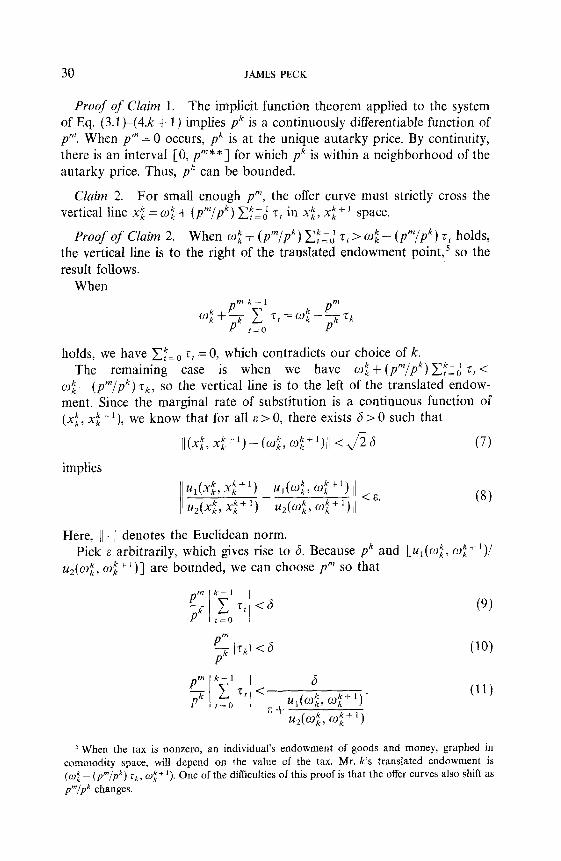
Proof of Claim 1. The implicit function theorem applied to the system of Eq. (3.1)-(4.k f 1) implies pk is a continuously differentiable function of p”. When pm = 0 occurs, pk is at the unique autarky price. By continuity, there is an interval [0, pm** ] for which pk is within a neighborhood of the autarky price. Thus, p” can be bounded.

Claim 2. For small enough pm, the offer curve must strictly cross the vertical line xi = 6.9; + (pm/#) cf;d T, in xt , IX; + ’ space.

Proof of Claim 2. When 0:: + (pm/p”) c:rd zt > 02 - (p”/pk) z, holds, the vertical line is to the right of the translated endowment point,5 so the result follows.

When mk-1 m

o,$+'F ; ,,=f$-p~~k

f 0

holds, we have C:=, z, = 0, which contradicts our choice of k. The remaining case is when we have CL$ + (p”‘/pk) 2”;:: z, -=z

o:- (p”‘/p”) zk, so the vertical line is to the left of the translated endowment. Since the marginal rate of substitution is a continuous function of (xi, x:+9, we know that for all s>O, there exists 6>0 such that

ll(x~,~::+‘)-~~kk,~~+l)/I 4s (7)

implies

Here, II.11 denotes the Euclidean norm. Pick e arbitrarily, which gives rise to 6. Because pk and [u,(o,k, oE+r)/

u,(Q$, u.$+ ‘)I are bounded, we can choose p” so that

(11)

5 When the tax is nonzero, an individual’s endowment of goods and money, graphed in commodity space, will depend on the value of the tax. Mr. k’s translated endowment is (O:-(pm/Pk)rk,okk+l). 0 ne of the difkulties of this proof is that the offer curves also shift as pm/p” changes.


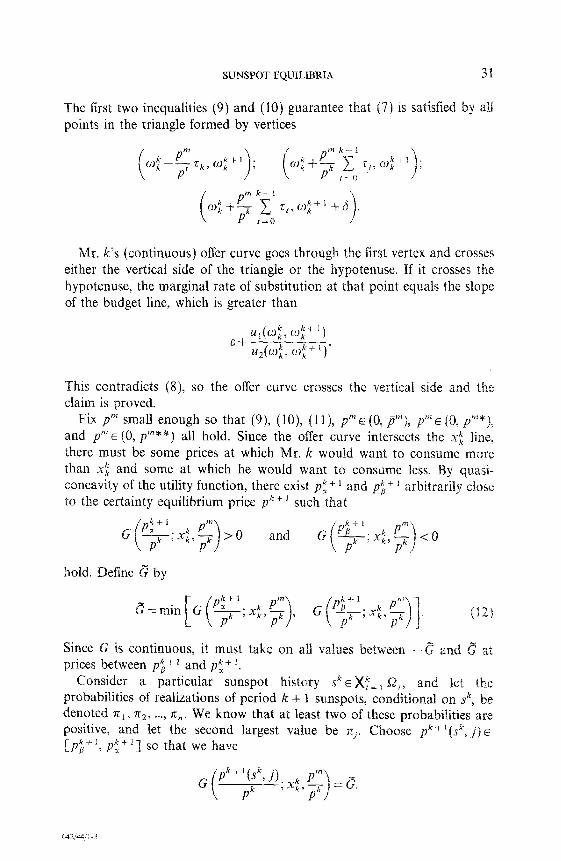
The first two inequalities (9) and (10) guarantee that (7) is satisfied by ah points in the triangle formed by vertices

Mr. k’s (continuous) offer curve goes through the first vertex and crosses either the vertical side of the triangle or the hypotenuse. If it crosses the hypotenuse, the marginal rate of substitution at that point equals the slope of the budget line, which is greater than

This contradicts (8), so the offer curve crosses the vertical side and the claim is proved.

Fix pm small enough so that (9) (lo), (ll), p”’ E (0, pm), p”’ E (0, pm*j9 and p”’ E (0, pm** ) all hold. Since the offer curve intersects the X: line, there must be some prices at which Mr. k would want to consume more than xf and some at which he would want to consume less. By quasi- concavity of the utility function, there exist pt + l and p); + ’ arbitrarily close to the certainty equilibrium price pkt ’ such that

and

hold. Define G by

Since G is continuous, it must take on all values between -G an prices between pg + 1 and pt+ I.

Consider a particular sunspot history sk E t probabilities of realizations of period k + 1 sunspo conditional on sk, denoted z,, x2, . . . . ‘I,. We know that at least two of these probabilities are positive, and let the second largest value be zj. C oose gk + ‘(,yk, j) E

k+l L-P/3 2 Pi+’ 1 so that we have

G P”“bkyj);xk pm Pk

kr -i; =?%,

P

64?,‘44; : -3

32 JAMES PECK

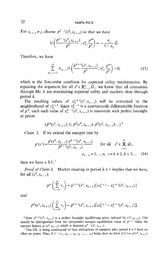
For sk+, fj, choose pk”(sk, Sk+l) so that we have

k+l(SkJk+l) k P” Pk

; x,,T P >

= -&“.

Therefore, we have

i 7csk+, G %+I=1

pk+“~~sk+l’;x~;~)=~, (13)

which is the first-order condition for expected utility maximization. By repeating the argument for all sk E X-r=, Q2,, we know that all consumers through Mr. k are maximizing expected utility and markets clear through period k.

The resulting values of xi+ I(.@, sk+ ,) will be contained in the neighborhood of xi + l. Since xk k+’ is a continuously differentiable function of pn*, each such value of xf+ ‘(sk, sk+ 1) is consistent with perfect foresight at prices

Claim 3. If we extend the sunspot tree by

s,+,=t ,,.., ?t, t=k+2,k+3 ,... (14)

then we have a S.E.7

Proof qf Claim 3. Market clearing in period k + 1 implies that we have, for aI1 (Sk, Sk + 1),

and

b Here fik + I(?, sk+ ,) is a perfect foresight equilibrium price, indexed by (sk, sk + ,). This should be distinguished from the (proposed) sunspot equilibrium value of pk+’ when the sunspot history is (?, skfl), which is denoted #+‘(s’, sksi).

‘This S.E. is being constructed so that realizations of sunspots after period k + 1 have no effect on prices. Thus, ifs’ = (sl, sz, . . . . sk, sk + ), . . . . sI) holds then we have p’(s’) = p’(sk, sk + ,).


Therefore, we have

Given the realization s/, + r E Qk+, and the history sh, constraint for t > k is

r. t’s budget

pf(sk, s,+,)[x;-w;] + pr+ysi, sk+lj[x;+l -o;+‘] = -JPTr. 616)

Substituting (14) and (15) into (16), we find t at the budget constraint faced by Mr. t in the sunspot economy is equivalent to

This -is the same constraint as that faced by I-. t under the perfect foresight equilibrium indexed by (sk, s k + 1 ). Therefore he demands the same amount here in the proposed SE. as he s in the perfect foresight equilibrium, and markets continue to clear. choosing prices according to (14) we have shown that the utility-maximizing consumption levels also clear markets, so (p”; 1; p’; . . . . pk; pk+‘(sk, s,,,); +2(sk3 skLl); . ..) is ;p S.E. where we let (s’, sk+ ,) run over the entire set

For K > k, we can branch the tree again i e have c;=O T , # 0 and p”’ small enoughs For any sunspot history sK E _ 1 Qi, there exist p; + ’ an pi+ l where

and

Let the probabilities of period K + 1 sunspots, conditional on sr, bs

denoted nl, rc2, . . . . rc,. By the argument used above, there are prices arbitrarily close to pK + ‘(sk, s k+l) defined in (14), w

* If the initial choice of p” was too high, we can choose a lower p” and redo the proof up until now.

34 JAMES PECK

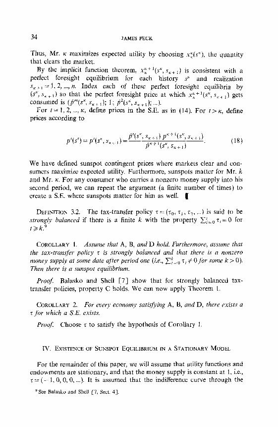
Thus, Mr. K maximizes expected utility by choosing x;(sK), the quantity that clears the market.

By the implicit function theorem, x;+I(P, s,+ r) is consistent with a perfect foresight equilibrium for each history s” and realization $A-+1 = 1, 2, .,., n. Index each of these perfect foresight equilibria by (sK, s,+r) so that the perfect foresight price at which $+‘(.sK, s,+r) gets consumed is (p”(.rK, s,+ ,); 1; B2(sX, s,+ r); . ..).

For t = 1,2, . . . . K, define prices in the S.E. as in (14). For t > rc, define prices according to

We have defined sunspot contingent prices where markets clear and consumers maximize expected utility. Furthermore, sunspots matter for Mr. k and Mr. K. For any consumer who carries a nonzero money supply into his second period, we can repeat the argument (a finite number of times) to create a SE. where sunspots matter for him as well. a

DEFINITION 3.2. The tax-transfer policy z = (lo, zr, r2, ,..) is said to be strongly balanced if there is a finite k with the property C:=0 r,=O for t>k.9

COROLLARY 1. Assume that A, B, and D hold. Furthermore, assume that the tax-transfer policy z is strongly balanced and that there is a nonzero money supply at some date after period one (i.e., Cf=, z, # 0 for some k > 0). Then there is a sunspot equilibrium.

ProoJ: Balasko and Shell [7] show that for strongly balanced tax- transfer policies, property C holds. We can now apply Theorem 1.

COROLLARY 2. For every economy satisfying A, B, and D, there exists a z for which a S.E. exists.

Proof: Choose r to satisfy the hypothesis of Corollary 1

IV. EXISTENCE OF SUNSPOT EQUILIBRIUM IN A STATIONARY MODEL

For the remainder of this paper, we will assume that utility functions and endowments are stationary, and that the money supply is constant at 1, i.e., z = (- 1, 0, 0, 0, . ..). It is assumed that the indifference curve through the

9 See Balasko and Shell [7, Sect. 41.


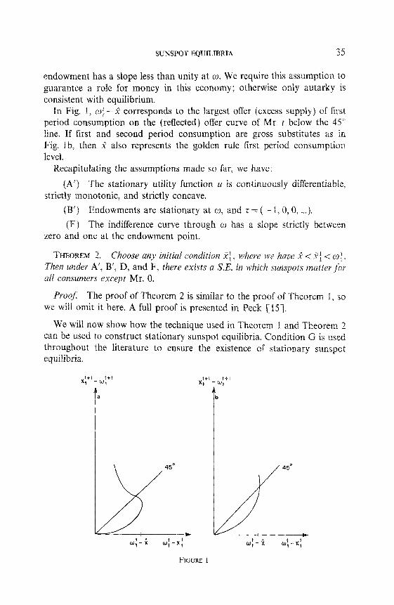
endowment has a slope less than unity at o. We require this assumption to guarantee a role for money in this economy; otherwise only autarky is consistent with equilibrium.

In Fig. 1, w: - 2 corresponds to the largest offer (excess supply) of first period consumption on the (reflected) offer curve of Mr. f below the 45” line. If first and second period consumption are gross substitutes as in Fig. lb, then 1 also represents the golden rule first period consumption level.

Recapitulating the assumptions made so far, we have:

(A’) The stationary utility function u is co~ti~uo~~ly differentia strictly monotonic, and strictly concave.

(B’ ) Endowments are stationary at o, and r = ( - 1, 0, 0, .~. ).

(F) The indifference curve through o has a slope strictly betwee zero and one at the endowment point.

THEOREM 2. Choose any initial condition Xt, where we have 2 < .Y: < 0:. Then under A’, B’, D, and F, there exists a S.E. in which sunspots matterfor all consumers except Mr. 0.

ProojY The proof of Theorem 2 is similar to the proof of Theorem 1, so we will omit it here. A full proof is presented in Peck 11151.

We will now show how the technique used in Theorem 1 and Theorem can be used to construct stationary sunspot equilibria. Condition G is use throughout the literature to ensure the existence of stationary sunspot equilibria.

FIGURE I

36 JAMESPECK

(G) First and second period consumption are gross complements and the golden rule equilibrium is locally stable.

THEOREM 2a. Under A’, B’, D, F, and G, there is a stationary sunspot equilibrium (where consumption is a function of the current realization on/y) for some Markov process.

ProoJ: Conditions F and G guarantee that the offer curve is backward bending and has a slope between - 1 and 0 where it intersects the 45” line (as in Fig. la). Choose two points, (a, a) and (b, b) with a < b, on the 45” line, near the intersection with the offer curve but on opposite sides of the intersection. Consider the square defined by the vertices (a, a), (a, b), (b, b), and (b, a). Let a and b be chosen so that (a, 6) is above the offer curve and (6, a) is below the offer curve.

The proposed equilibrium is given as follows;

pl = 1, p”=a, s1 =a

P’IP <+I _

- 1 when sI=st+, =c1,

= b/a when ~,=a and s~+~=/I,

= 1 when s~=s,+, =/3,

= a/b when sI=p and sI+l=cI,

x:(a) = 0: -a, x-,(a)=co:-, +a,

x;(p) = co; - b, x:eI(B)=w:-l+b.

When s, = ~1, we have G(p” ‘(a)/~‘; o;- a) < 0 and G(p’+‘(P)/p’; a$--a)>O. When s<=/?, we have G(p’+‘(a)/p’; o:-b)<O and G(p’+‘(/l)/p’; o: - b) > 0. There is a stationary transition matrix I7 satisfying Eq. (13), which completes the construction of the equilibrium. 1

V. SOME PROPERTIES OF SUNSPOT EQUILIBRIA

THEOREM 3. In a S.E. for which we have p” 3 0 and A’, B’, and F, then for any sunspor history, .2 d xi < co: must hold.

Proof. If we have xi I=- wi then money has a negative value in period t. Either pm < 0 or pf < 0 must occur. By hypothesis, pm > 0 holds, and negative equilibrium commodity prices are inconsistent with monotonicity. Therefore, x: Go; must hold.

Now we show that xi < P leads to a contradiction. By the definition of R, either the (reflected) offer curve is always to the left of w: -xi or it takes that value strictly above the 45” line.


Tn the former case, G(pri’/p’; xi) > 0 is true for all ,“~/JI’~ which contradicts expected utility maximization.

In the latter case, there exists E > 0 such that:

(1) the point (13: -xi, 01: -xi + E) is on the offer curve;

(2) (0:-x;, z) is on the offer curve implies we have z 3 o: -xi + E.

At any price ratio p’/~‘+~, where we have

then

holds. For a S.E. to exist there must be at least one path with strictly positive probability for which we have

P’ -?Ti>

U;-X;+E

P 0:-x; ’

It follows that x:+ 1 -o{+ r 2 w: - x: + E holds true along that path. market clearing in period t + 1, o: z : - xi z : z w: - xi + E holds.

If the offer curve is always to the left of ~:--x;+E, we are Otherwise, there exists E’ > 0 such that:

(1) the point (w:=:-x:=:,w:=:-xX:=:+E’) is on

(2) ;w:::-x:::, z) is on the offer curve imphes we x:;: -FL.

rough the origin can intersect the offer curve only once, which implies

(#+1 if1 -x:;:+&’ o;-x;+&

&)r+1-y+1 >

t+1 ICl 0:-x; .

The fact that o: z i - x; z : > o; - xi implies F’ > E. At any price ratio ~~‘+l,/p’+~, where we have

P Iti t+1

r+2< 0*+1

tt1, t -X,+I-l-E

P 1+1 r+1 ’

u~+l-x,+l

then

38 JAMES PECK

occurs. For a S.E. to exist there must be at least one path with strictly positive probability for which we have

P *+t mt+1 -x’+l

-7y33 t+1 r+l+E’

P ~‘+l~x’+l .

1+1 1+t

Along that path, x;~~--u:;~>Izo;;:-x;;~ + E’ must hold. Therefore, we have x;~:--o;$:>~;;~-x;;: + E 3 I$ - x: f 2s. Market clearing implies (#+2

tt2 - xi: z 3 CO’ - xi + 2s. Repeating the same argument k - 2 more times, there must be a Lath with each branch having strictly positive probability

for which we have

By making k large enough, there must be a path of finite length that violates market clearing. The probability of the entire path, given the sunspot history up to period t, is the product of a finite number of strictly positive numbers, which must itself be positive. We have a contradiction, so 2z.x; holds. 1

This restriction on paths consistent with equilibrium is related to the literature on decentralized capital accumulation.” In those models, there are price paths which are period-by-period consistent with rational behavior but which eventually drive some prices down to zero. This contradicts market clearing, so the path cannot be an equilibrium. Here we have paths in which consumers behave rationally, but where p’+ l/pt is being driven down. Eventually a consumer will be expected to supply more than his entire endowment, or else the offer curve bends backwards, in which case the path is inconsistent with equilibrium. The restriction that we have fdxido: applies to sunspot equilibria just as it applies to non- sunspot equilibria.

The asymptotic properties of perfect foresight equilibria are fairly well known. Convergence to autarky, convergence to the golden rule steady state, chaos, and cyclical behavior are all possible, depending on the offer curve. It is more difficult to describe the asymptotic properties of sunspot equilibria because there are potentially an infinite number of paths rather than just one.

It is clearly possible in a S.E. to reach autarky with probability one, or to reach the golden rule steady state with probability one. Azariadis [2] has shown that when sunspots form a stationary first-order Markov process, random cycles can result, in which the economy avoids autarky and the golden rule steady state. There are equilibria in which some paths reach autarky and others reach the steady state, while some paths cycle or

lo See Shell, Sidrauski, and Stiglitz [19], especially Section 3


exhibit chaos. Without placing restrictions on the offer curves, the only general statement about asymptotic behavior seems to be that consumption must stay within the bounds established by Theorem 3.

VI. WELFARE PROPERTIES

An appropriate measure of welfare for sunspot equilibria is ex ante expected utility. Thus, an allocation (possibly contingent on sunspots) is Pareto optimal if there is no other allocation yielding at least the same expected utility to all agents and strictly higher expected utility to at least one agent. All expectations are taken in period one.

THEOREM 4. Sunspot equilibria are not Pareto optimal.”

Proof Consumer t’s ex ante expected utility in a SE. is given by

“2 = 1 S) = 1 st=l s,+,=l Consider the allocation { (Xj, 2;’ “) > ,“= 1, which gives each agent his expected consumption, independent of sunspots. Mr. 0 gets the same utility that he gets in the S.E. For t >, 1, u(Zi, Xi+ ‘) equals

Because utility is a strictly concave function, the expression in Eq. (20) is strictly greater than the expression in Eq. (19). It remains to show that ((Xi, X:+‘))y=r is feasible.

” This theorem was first proved for a static model by Cass and Shell 191. It was also stated in a more general overlapping generations context by Balasko [4]. He was not assuming that consumers have von-Neumann Morgenstern expected utility functions, and the proof was somewhat intricate. I am presenting the proof in this simpler framework to high&&t its essential features.

40 JAMES PECK

Therefore, ((G X:+Y}rm=l is feasible and dominates the sunspot equilibrium. 1

It is well-known fact that non-sunspot equilibria are often Pareto inefhcient.r2 This fact calls for a comparison between the sunspot equilibria for a given initial condition and the non-sunspot equilibria for the same initial condition. It is not surprising that the non-sunspot equilibrium can dominate all sunspot equilibria. However, there are also economies for which a sunspot equilibrium dominates the unique non-sunspot equilibrium with the same initial conditioni Thus, if a benevolent social planner is stuck with a bad initial condition, he may find it useful to introduce randomness to a previously deterministic economy.

Examples of sunspot equilibria that cycle can be constructed without requiring the offer curve to bend backwards.14 The economy follows a tirst- order Markov process with a stationary N x N transition matrix. However, it should be noted that there is a major qualitative difference between the examples with gross substitutability and those of Azariadis [2], with gross complementarity. As time unfolds here, the economy eventually reaches one of the steady states; the probability of reaching the golden rule depends on where the economy starts. Thus, the impact of sunspots eventually disappears. l5 In the gross complement examples, the consumption levels can be picked so as not to include either steady state, so sunspots will always affect the economy without dying out.

I2 This point was made in Samuelson [ 161. Balasko and Shell [5, especially Sect. 41 show that all equilibria are weakly Pareto optimal in the sense that they cannot be dominated by allocations differing from the equilibrium allocation by a finite number of components.

‘3 This type of SE. was first put forth by Azariadis and Guesnerie [3 J. See also Peck [15, p. 55-J.

14An example is worked out in Peck [15, p. 591. r5By eventually I mean that the probability of the economy reaching one of the steady

states by period t approaches 1 as t approaches infinity. At the steady states, sunspots can have no effect.

SUNSPOT EQUILIBRIA

VII. CONCLUDING REMARKS

By allowing arbitrary stochastic processes to cause sunspot equilibria, we are able ts incorporate the equilibria of Shell [Is] and Azariadis (21 into the same framework. This more general view of sunspots allows us lie prove the existence of equilibria under assumptions less restrictive than those used previously. However, sunspot equilibria will no longer necessarily be stationary. Even when they are constructed to be stationary, the impact of sunspots may die out unless preferences are restricted somewhat. e have seen that sunspot equilibria are not Pareto optimal in terms of ex ante expected utility, although they may dominate the corresponding non- sunspot equilibrium.

This model can be extended in several interesting directions. With more than one commodity per period, sunspots can affect the general price level and relative prices. It seems that sunspot equilibria will be even mire prevalent than they are in the one-commodity model.

One theme of this and other work on sunspots is that an open-en future creates its own uncertainty. Not even rational expectations and completely foreseen market fundamentals can destroy the impact of &logical variables. The vast multiplicity of sunspot equilibria creates problem of not knowing which equilibrium will arise. A promising line of future research is to analyze mechanisms which coordinate expectatloras, whether by consumer interactions or focal points.

When intrinsic uncertainty is added to the model, interesting com- plications arise. Small changes in realizations of the fundamentals coui have a large impact on the economy if people allow ihem to affect their expectations. Budget deficits, for example, could influence the eco~am~ directly through fundamentals and indirectly through ex

REFERENCES

1. R. AUMANN, Subjectivity and correlation in randomized strategies, J. Math. Econ. 1 (19741, 67-96.

2. C. AZARIADIS, Self-fulfilling prophecies, J. &on. Theory 25 (1981). 3%396. 3. C. AZARIADIS AND R. GUESNERIE, Sunspots and cycles, Rev. Econ. Stud. 53 (1986),

No. 176, 725-738. 4. Y. BALASKO, Extrinsic uncertainty revisited, J. Econ. Theory 31 (1983), 203-210. 5. Y. BALASK~ AND K. SHELL, The overlapping-generations model. I. The case of pure

exchange without money, J. Econ. Theory 21 (1980), 281-306. 6. Y. BALASKO AND K. SHELL, The overlapping-generations model. II. The case of pure

exchange with money, J. Econ. Theory 24 (1981), 112-142. See also Erratum, J. Econ. Theory 25 (1981X 471.

42 JAMES PECK

7. Y. BALASKO AND K. SHELL, Lump-sum taxes and transfers: The overlapping-generations model with money, in “Essays in Honor of Kenneth J. Arrow, Volume II: Equilibrium Analysis” (W. Heller, R. Starr, and D. Starrett, Eds.), Chap. 5, pp. 121-153, Cambridge Univ. Press, Cambridge, England, 1986.

8. D. CASS, M. OKUNO, AND 1. ZILCHA, The role of money in supporting the Pareto optimahty of competitive equilibrium in consumption-loan type models, J. &on. T,+eorJ~ 20 (1979), 41-80.

9. D. CA%~ AND K. SHELL, Do sunspots matter? J. Polk ECO~Z. 91 (1983), 193-227. 10. G. DEBREU, “Theory of Value,” Wiley, New York, 1959. 11. R. FARMER AND M. WOODFORD, “Self-fulfilling Prophecies and the Business Cycle,”

CARESS Working Paper No. 84-12, 1984. 12. D. GALE, Pure exchange equilibrium of dynamic economic models, J. Econ. Theory 6

(1973), 12-36.

13. R. E. LUCAS, JR., Expectations and the neutrality of money, J. Econ. Theory 4 (1972), 101-124.

14. J. M. KEYNES, “The General Theory of Employment, Interest, and Money,” Harcourt Brace Jovanovich, New York/London, First Harbinger Edition, 1964.

15. J. PECK, “Essays in Intertemporal Economic Theory,” Dissertation in economics, Univer- sity of Pennsylvania, Philadelphia, 1985.

16. P. A. SAMUELSON, An exact consumption-loan model of interest with or without the social contrivance of money, J. Polk Econ. 66 (1958), 467482.

17. K. SHELL, Notes on the economics of infinity, J. Polk Econ. 79 (1971), 1002-1011. 18. K. SHELL, Monnaie et allocation intertemporelle, mimeograph, CNRS Seminaire

d’bconometrie de Roy-Malinvaud, Paris, November 1977. [Title and abstract in French, text in English]

19. K. SHELL, M. SIDRAUSKI, AND J. E. STIGLITZ, Capital gains, income, and saving, Rev. Econ. Stud. 36 (1969), 15-26.

20. S. SPEAR, Sufficient conditions for the existence of sunspot equilibria, J. Econ. Theory 34 (1984), 36G370.

21. S. SPEAR, Rational expectations in the overlapping generations model, J. Econ. Theory 35 (1985), 251-275.

22. S. SPEAR AND S. SRIVASTAVA, Markov rational expectations equilibria in an overlapping generations model, J. Econ. Theory 38 (1986), 36-62.

on the existence of sunspot equilibria in an overlapping generations model

Documents