On the Estimation of Parameters ofVariograms of Spatial Stationary Isotropic

Random Processes

Sourav Das, Tata Subba Rao & Georgi N. Boshnakov

First version: 21 May 2012

Research Report No. 2, 2012, Probability and Statistics Group

School of Mathematics, The University of Manchester

On the estimation of parameters of variograms of spatial stationary

isotropic random processes

Sourav Das∗, Tata Subba Rao†and Georgi N. Boshnakov‡

January 20, 2012

Abstract

In this paper we consider the estimation of the variogram using the method of weighted least squaresand in the process we propose two alternative set of weights. We study the asymptotic sampling propertiesof these estimators and compare their efficiencies both analytically and through simulations. To illustratethe above methods, we consider daily rainfall across Switzerland measured at 467 locations on a singleday. We propose an alternative variogram for this data and study the efficiency of this variogram inprediction (’kriging’) compared to other variograms used in literature.

Keywords: weighted least squares; variogram estimation; matern class; wave variogram

1 Introduction

Let Z(s); s ∈ D ⊂ R2 be a random field (or random process) observed on a plane in a probability space(Ω,B, P ) for a fixed event ω, where D is a fixed and continuous open set. The objective is to predictthe process at some fixed location s0 based on a sample of observations of the process at n fixed locationss1, s2, ..., sn. Let E[Z4(si)] < ∞. We say that the process Z(si) is weakly or second order spatiallystationary if its mean is a constant and the covariance is a function of spatial differences only, i.e.

E[Z(si)] = µ

Var[Z(si)] = σ2 <∞Cov[Z(si), Z(sj)] = C(si − sj).

(1)

Further, if C(si − sj) is a function of the spatial distance (the Euclidean norm), ‖si − sj‖, then the processis said to be isotropic1. In this case Cov[Z(si), Z(sj)] = C(‖si − sj‖).

Sometimes the random process might not be stationary but the increments Z(si) − Z(si + h) mightbe. A process for which this property holds is said to be intrinsically stationary. More precisely, the processZ(s) is said to be intrinsically stationary if

E[Z(si)] = µ

2γ(h) = Var[Z(si)− Z(sj)](2)

where h = si− sj and (si, sj) ∈ N(h). Here N(h) = (si, sj) : si− sj = h; i, j = 1, 2, ..., n denotes the set ofall pairs of locations having lag difference h. 2γ(h) is defined to be the variogram while γ(h) is defined as the

∗Correspondence to: Sourav Das, University of Manchester (UK) and CR Rao AIMSCS(Hyderabad,India); E-mail:sourav2.das@googlemail.com†School of Mathematics, University of Manchester(UK) and CR Rao AIMSCS(Hyderabad, India)‡School of Mathematics, University of Manchester(UK)1In earth science prediction problems isotropy or directional symmetry of the random process is frequently assumed. Though

for many geostatistical processes (such as mining) it is expected, there are many physical phenomena where it should be properlyassessed and treated accordingly. The main advantage of this assumption is that it renders the construction of a very flexiblegeneral class of covariance/variogram function which explains the association structure of a wide variety of naturally occurringphysical processes. For techniques used to deal with anisotropy one may refer to [16].

1

semi-variogram. Analogous to covariance functions (or covariograms as referred to in the spatial literature),a function is a valid variogram if and only if it is conditionally negative definite ([5, p.86]), that is if and onlyif,

m∑i=1

m∑j=1

aiaj2γ(si − sj) ≤ 0

for any finite number of spatial locations si : i = 1, 2, ...,m and real numbersai : i = 1, 2, ...,m satisfying

∑mi=1 ai = 0.

As stated earlier, one of our objectives is to predict Z(s) at a known location s0, given the observationsZ(s1), Z(s2), ..., Z(sn)′ . For convenience we assume EZ(s) = 0 for all s. We briefly outline the derivationof the widely used linear predictor (also called the kriging predictor). Let the predictor be of the formZ(s0) = λλλ

′Z(s), where λλλ = λ1, λ2, ..., λn

′. The object is to find λλλ such that,

Q(s0) = E[λλλ′Z(s)− Z(s0)]2 (3)

is minimum. By minimizing Q(s0) with respect to λλλ, we can easily show that Z(s0) = σσσ′(s0, s)Σ−1Z(s),

where σσσ′(s0, s) = E(Z(s0)Z(s)) and Σ = E[Z(s)Z

′(s)] is the covariance matrix. The minimum of Q(s0) is

minQ(s0) = σ2 − σσσ′(s0, s)Σ−1σσσ(s0, s). In the geostatistics literature this is also referred to as the kriging

variance. We note that Q(s0) can be rewritten in terms of the variogram by noting that

σσσ(s0, s) = σ21− 1

2Γ(s0, s). (4)

where Γ(s0, s) is the corresponding matrix of variograms. We can thus rewrite Q(s0) given in (3) as

Q(s0) = −1

2λλλ

′Γλλλ+ λλλ

′Γ(s0, s). (5)

We now minimize Q(s0) with respect to λλλ subject to the constraint λ′1 = 1 (accounting for unbiasedness of

the predictor Z(s0)), by considering

Q′(s0) = Q(s0)−m(λ

′1− 1). (6)

By differentiating Q′(s0) with respect to λλλ we get

λ′ = (γ + 11− 1′Γ−1γ

1′Γ−11)Γ−1

m = −1− 1′Γ−1γ

1′Γ−11(7)

The minimum of Q′(s0) is

σ2ok(s0) = C(0)− σ′Σ−1σ +

[1− 1′Σ−1σ]2

1′Σ−11. (8)

The above equations demonstrate that the precision of prediction of a random process at unobservedlocations depends on the underlying variogram of the process. The above equations could also be expressedin terms of the covariogram C(si − sj) but in the context of geostatistics the variogram is usually favouredas the measure of dependence. Cressie [5, Sec 2.4] provides a comparison between the use of variogram andthe covariogram in spatial statistics.

But the variogram (or the covariance) of a random process is usually unknown. Consequently the problemof estimating the variogram is central to the problem of spatial prediction. Matheron ([13]) defined the earliestunbiased non-parametric variogram estimator for a fixed lag h, as

2γ(h) =1

|N(h)|∑N(h)

[Z(si)− Z(sj)]2,

where |N(h)| is the number of distinct pairs of locations, (si, sj), from the set N(h), defined above. It is nowreferred to as the classical variogram estimator. But the Matheron classical variogram estimator defined above

2

does not ensure non-negative definiteness and consequently its use in kriging might even lead to negative meansquare prediction errors ([5, Sec. 2.5]). Moreover, we note that even though the classical variogram estimatorcan estimate the variogram for any two locations (si, sj) for which observations (Z(si), Z(sj) are available, itcannot estimate the variograms γ(s0 − si), for i = 1, 2, ..., n. Thus we require a smoothing function that canevaluate the variogram at any arbitrary pair of locations. A classical approach of circumventing this problemis to consider parametric variogram functions that satisfy the desired conditional negative definiteness and’fit’ the sample variogram to such functions by estimating the parameters through different optimizationmethods. In this paper we consider parametric estimation of the parameters of variogram functions forspatial random processes.

Among the estimation techniques there are two broad categories: the least squares methods and maximumlikelihood methods. There are three principal least squares methods that are often used. These are: Ordi-nary Least Squares (OLS), Weighted Least Squares (WLS) and Generalized Least Squares (GLS). The leastsquares methods are attractive due to their simplicity of application, non-parametric nature and geometricinterpretation. The well known likelihood based methods include methods such as Maximum Likelihood(ML), Generalized Estimating Equations (GEE), Restricted Maximum Likelihood (REML) and Quasi Like-lihood Methods (QL). Most of the likelihood methods originate from the assumption of Gaussianity but thenshown to work under more general conditions.

Here we do not impose any distributional assumptions on the spatial process and thus opt for WLS asthe variogram fitting method. For a review of different methods of variogram estimation see Cressie[5, Sec.2.6].

Let Z(s1), Z(s2), ..., Z(sn)′ be the sample of size n observed at n fixed locations for the second orderstationary process Z(s). Let 2γ(h, θθθ) be a valid theoretical variogram to which we want to fit the classicalvariogram estimator for this process, where θθθp×1 ∈ Θ ⊂ Rp is the vector of unknown parameters and Θis an open parameter space. A widely used class of parametric variograms is the three parameter Maternfamily that we discuss later. According to the GLS technique parameters are chosen subject to minimizationof a weighted sum of squares.

Q(θθθ) = g′(θθθ)V (θθθ)g(θθθ), (9)

where g(θθθ) = 2γ(h1)−2γ(h1, θθθ), ..., 2γ(hk)−2γ(hk, θθθ)′

and V (θθθ), the weight matrix, which is usually takenas the inverse of the dispersion matrix of the sample variogram, Eg(θθθ)g

′(θθθ). In this way sample variograms

with small variance have more weight in variogram fitting than sample variograms with large variance. Dueto computational difficulties usually a diagonal weight matrix is considered and the method is referred to asWLS. In this paper we study the effects of using different weight functions on the parameter estimation of θθθunder WLS.

In the following we propose different criteria which we minimize with respect to θθθ to obtain optimalestimates. First we consider the widely used criterion

Q1n(θθθ) =k∑i=1

[2γ(hi)− 2γ(hi, θθθ)]2v1i(θθθ),

where v1i(θθθ) =|N(hi)|

2(2γ(hi, θθθ))2, i = 1, ..., k.

(10)

Here k denotes the number of distinct lag distances at which the sample and theoretical variograms arecomputed.

Cressie[4] and further Zimmerman et al. [19] (through empirical comparisons) favour the use of v1i(θθθ)which has since become the commonly used weight function. v1i(θθθ) was proposed by Cressie [4]. We brieflyprovide the motivation for considering the above. If the random process Z(s) is Gaussian with a constantmean, then Z(s + h) − Z(s) v N(0, 2γ(h)). This implies that Z(s + h) − Z(s)2/2γ(h, θθθ) v χ2

1, thusVar

[Z(s + h)− Z(s)2

]= 2(2γ(h, θθθ))2 Now, assuming that the ”between-lag” covariances of the variogram

clouds are weak, that is

Cov[Z(si + hl)− Z(si)2, Z(sj + hm)− Z(sj)2

]w 0,

for all i, j = 1, 2, ...n and l,m = 1, 2, ..., k the above implies that, Var[2 ˆγ(hi)] w 2(2γ(hi, θθθ))2/|N(hi)|. This

lead Cressie to propose v1i(θθθ) as the weight function, shown in (10). The method is simple yet powerful

3

provided that the assumptions of Gaussianity and covariance are valid. But apart from the Gaussianityassumption (which is relaxed later) the assumption on the covariance is quite strong for many geostatisticalprocesses. Consequently this weight function, despite being an improvement over the ordinary least squares,leaves scope for further improvement on the efficiencies of parameter estimators. Also, the fact that theweight function depends on the parameters θθθ leads to biased generalized estimating equations (see e.g [7, p.109]) for Q1n(θθθ).

Here we propose two alternative weight functions, v2i(θθθ) and v3i(θθθ) as improvements in these regards andillustrate that even within the framework of WLS we can improve the efficiency. The alternative criteria wepropose are

Q2n(θθθ) =

k∑i=1

[2γ(hi)− 2γ(hi, θθθ)]2v2i(θθθ)

Q3n(θθθ) =

k∑i=1

[ln 2γ(hi)− ln 2γ(hi, θθθ)]2v3i(θθθ) (11)

where the weight functions are

v2i(θθθ) = |N(hi)|/

1

|N(hi)|∑N(hi)

[Z(sl)− Z(sm)2 − 2γ(hi)]2

v3i(θθθ) =

|N(hi)|2

(12)

The justifications for the above considerations are as follows. First note that v1i(θθθ) is inversely proportionalto 2(2γ(hi, θθθ))

2; which we know from above, is the variance of Z(s + hi) − Z(s)2. In constructing v2i(θθθ)we replace this unknown parametric function by its sample counterpart.

Thus v2i(θθθ) is the inverse of the sample estimator of Var[2 ˆγ(hi)]. It doesn’t depend on θθθ. Later we present acomparative analysis of the standard errors and mean squared errors of estimates of θθθ, obtained from WLSusing v2i(θθθ) and v1i(θθθ).v3i(θθθ) on the other hand is based on the theory of variance stabilization. We have already mentioned thatthe weight function v1i(θθθ) is based on the assumption of Gaussianity. Cressie, later relaxes the assumptionof Gaussianity but recommends the use of v1i(θθθ) for a broader class of random processes for which

Var[2 ˆγ(hi)] ∝ (2γ(hi, θθθ))2.

We propose using the variance stabilizing transformation to make the above weight function independent ofthe parameter vector θθθ and investigate the properties of the estimators thus obtained. Since the variance isassumed to be proportional to the square of the expectation of 2γ(hi), it is well known that the logarithmic

transformation of 2γ(hi) has a variance proportional to 2|N(hi)| . Thus, we use |N(hi)|

2 as the weight function,

v3i(θθθ), in Q3n(θθθ).The parameter free weight function v3i(θθθ) also makes the estimating equations asymptotically unbiased

(see Appendix). But as we show later in Section 4, using a general result obtained by Lahiri et al. [11], themain advantage of using v3i(θθθ), is that we obtain estimators with smaller asymptotic variance. In order toobtain the asymptotic statistical properties of estimators we first need to study the statistical properties ofthe variogram estimator itself.

In Section 2 we first establish weak convergence of sample variogram (which is followed by the almost sureconvergence). In Section 3, results stated in Section 2 are used to show strong convergence and asymptoticnormality of the parameter estimators of theoretical variogram function while using the three different weightfunctions. In Section 4 we compare the asymptotic variances of the parameter estimators obtained fromQ1n(θ) with that of Q3n(θ). In Section 5 we present the simulation results; where we compare the threedifferent sets of estimators for random processes generated from three different distributions and discussthe mean square errors and biases of the parameter estimators. The objective of this empirical study is tocompare the robustness of the methods when there is departure from Gaussianity. In Section 6 results ofanalysis of two real data sets are presented.

4

2 Weak and strong convergence of the classical variogram estima-tor

In this section we establish consistency properties of the classical variogram estimators which would berequired in demonstrating the asymptotic Gaussianity and consistency of the parameter estimators. Thedetails of the proof are provided in the appendix.

2.1 Weak convergence

Theorem 1. Let Z(s); s ∈ D ⊂ R2 be a stationary random field. The process is observed at n fixedlocations on the domain D. We assume that the domain is increasing but also allows for ”infilling” (we willlater provide details of the method of sampling). We assume also that

1. B = supijV ar[Z(si)− Z(sj)]

2 <∞,

2. Km = limn→∞

n∑l=m+1

Cov[Z(sim)− Z(sjm)2, Z(sil)− Z(sjl)2] <∞, for m = 1, 2, ..., n− 1,

3. K = supmKm.

Then

2γ(h)L2

→ 2γ(h) and hence, (13)

2γ(h)P→ 2γ(h). (14)

Proof. From the definition of variogram we know that

E[2γ(h)] = 2γ(h). (15)

Also using assumptions 1), 2) and 3) it can be easily shown that

V ar(2 ˆγ(hi))→ 0 as N→∞. (16)

Thus the sufficient conditions for mean square convergence of the variogram estimator are satisfied. Thisfurther implies that the classical variogram estimator converges in probability to the theoretical variogram.

2.2 Almost sure convergence

Next we deduce conditions for almost sure convergence of the classical variogram estimator, also referred toas strong convergence. We state two well known theorems that will be used later.

Theorem 2. Birkhoff’s Ergodic Theorem: Let Xt(ω)∞1 be a stationary, ergodic, integrable sequence and

Sn(ω) =

n∑t=1

Xt(ω). Then

limn→∞

Sn(ω)

n= E(X1, ω), almost surely(a.s) (17)

(for proof see e.g, [2]). The next result (Theorem 3, which we only state here) allows us to apply Birkhoff’stheorem to a large class of functions (see e.g [2]).

Theorem 3. Suppose that Zt is an ergodic sequence (for example iid random variables), g : R∞ → R is ameasurable function and Yt = g(Zt, Zt−1, ..., ). Then the sequence Yt is an ergodic process.

Corollary 1. Let the random field Z(s); s ∈ D ⊂ R2 be ergodic. Noting that ˆ2γ(h) is a measurable functionof Z(s) we have

ˆ2γ(h)→ 2γ(h), a.s as n→∞. (18)

5

The proof follows almost immediately from Theorem 2, Theorem 3 and result (15).In the next section we present general results on asymptotic normality for the classical variogram estimator

and the distribution of parameter estimators of parametric variogram functions obtained using weighted leastsquares. The results were obtained by Lahiri et al. [11] under the mixed increasing domain sampling designwhich we describe next. It is based on the design proposed by Sherman and Carlstein [17].

3 Asymptotic normality of the variogram and parameter estima-tor

The sampling design is described in d dimensional Euclidean space Rd. We start with a basic rectangular in-teger lattice i, in d-dimensions. This is multiplied with a real valued diagonal matrix, ∆ = diag(δ1, δ2, ..., δd)

′,

to create Ld = ∆i : i ∈ Zd such that the lattice gets an increment of δi in the ith direction. This latticeregion is then superimposed over an increasing open set Rn = λn(−β, β]d;β ∈ (0, 1], λn → ∞ as n → ∞containing the origin, so that the intersecting sampling area, Ld

⋂Rn, can be generalized from a lat-

tice structure to a more general increasing continuous domain D acquiring many different convex as wellas non-convex shapes. Finally, to allow for infill sampling or allowing an increasing density of samplingwithin a subset of the above domain the above set is multiplied with a sequence of positive real numbershn such that hn ↓ 0. Thus it is assumed that the geostatistical process is observed at n fixed locationss1, s2, ..., sn

′ ∈ hnLd⋂Rn.

We now present the asymptotic properties of parameter estimators of parametric variogram functionsproduced under the above defined sampling scheme. We introduce below notations for matrices of variogramsand their derivatives. The definitions are generic and are applicable for all the three criteria vis-a-vis weightfunctions.

Let g(θθθ) denote the K × 1 vector of variogram differences (as defined after (9)). ∇lg(θθθ) denotes thevector of first derivatives of g(θθθ) with respect to the parameter θl, l = 1, 2, . . . , p. Then the matrix of firstderivatives is defined as D(θθθ) = [∇1g(θθθ),∇2g(θθθ), ...,∇qg(θθθ)](K×p).

Let V (θθθ)K×K denote the weight matrix for the least squares. We denote the ijth element of V (θθθ) byuij(θθθ) = Cov2γ(hi), 2γ(hj), i, j = 1, 2, ...,K.

The first order derivative of the weight matrix is defined by Vl(θθθ) = ∂∂θlV (θθθ), where the matrix elements

are ∇luij(θθθ) = ∂∂θluij(θθθ), for l = 1, 2, ..., p.

Then θθθ is estimated by minimizing

Qn(θθθ) = g(θθθ)′V (θθθ)g(θθθ) =

k∑i=1

k∑i=1

gi(θθθ)gj(θθθ)uij(θθθ)

with respect to θθθ = (θ1, θ2, ..., θp)′. We assume that θθθ0 is the true parameter value and θθθ is the unique

optimum value.We can now state the following theorems due to Lahiri et al. [11, Theorem 3.1, 3.2]. First we define and

discuss the following conditions which are required for the results.

Conditions

(i) The lag vectors chosen are such that the parametric variogram models are identifiable, that is, for any

ε > 0 there exists δ > 0 such that inf∑Ki=1(2γ(hi;θθθ1)− 2γ(hi;θθθ2))2 : ‖θ1θ1θ1 − θ2θ2θ2‖ ≥ ε > δ.

(ii) supγ(h;θθθ) : h ∈ R2, θ ∈ Θ < ∞ and γ(h;θθθ) has continuous partial derivatives of first order withrespect to θθθ.

(iii) The weight matrix V (θθθ) is positive definite for all θθθ ∈ Θ with sup|V (θθθ)|, |V (θθθ)−1| : θθθ ∈ Θ <∞. AlsoV (θθθ) is continuously differentiable.

(iv) Throughout the following discussion it is assumed that the true parameter value is θθθ0 and there exists a

unique optimum solution for Qn(θθθ), θθθn(say). Finally, for studying the asymptotic distributional prop-erties of parameter estimators under the mixed increasing domain sampling scheme we need conditionson moments and decay of the dependence measure.

6

(v) The number of sampling points in the boundary of the sampling region Rn is negligible.

(vi) Let T1, T2 be two arbitrary regions within the domain of observation D and let d(., .) be the l1 norm inRd. Define α(a, b) ≡ supα(T1, T2) : d(T1, T2) ≥ a, |T1| ≤ b, |T2| ≤ b, andα(T1, T2) ≡ sup|P (A

⋂B) − P (A)P (B)| : A ∈ FZ(T1), B ∈ FZ(T2), where FZ(T ) is the sigma field

generated by the random variables Z(s) : s ∈ T ⊂ Rd.We assume E|Z(0)|4+δ <∞ and for all a ≥ 1, b ≥ 1,

α(a, b) ≤ Ca−τ1bτ2 (19)

for some 0 < δ ≤ 4, C > 0, τ1 > (4 + δ)d/δ, and 0 ≤ τ2 < τ1/d.

The first part of the condition specifies that moments of up to (4+δ)th order exist. This is required sincewe are concerned with moments of variogram which are squared differences of random variables. Thesecond part is a mixing condition similar to the strong mixing condition, due to Rosenblatt [15], thatprovides the necessary bound on dependence structure of the spatial process. Das ([6]) has considereda commonly observed Gaussian spatial process to provide a heuristic explanation of the relationshipbetween the probabilistic condition (vi) and the corresponding covariance function.

Under the above conditions the following general results have been obtained by Lahiri et al.

Theorem 4. If 2γ(hi)a.s→ 2γ(hi;θθθ0)) as n → ∞ for i = 1, 2, ...,K, then, θθθn

a.s→ θθθ0. If instead 2γ(hi)p→

2γ(hi;θθθ0)) as n→∞, θθθnp→ θθθ0.

Earlier in Theorem 1 and Corollary 1 of Theorem 3 we have established the probability convergenceand almost sure convergence respectively of the classical variogram estimator. Thus combining the aboveconditions with Theorems 1 and 3 we obtain the corresponding asymptotic convergence of the parameterestimators θθθn. The next result demonstrates asymptotic Gaussianity of the estimator θθθn.

Theorem 5. Let the random field Z(s) be as defined before. Under the above conditions and using condi-tions for almost sure convergence of 2γ(hi), i = 1, 2, ..., k, if there exists a sequence of constants a(n) suchthat a(n)→∞ as n→∞ and

1. g(θθθ0)a.s→ 0,

2. D(θθθ0) is of rank q (i.e full rank),

3. a(n)g(θθθ0)D→MVN(0,W (θθθ0)),

then a(n)(θθθ − θθθ0)D→MVN(0,Σv(θθθ0)), where

Σv(θθθ0) = B(θθθ0)D(θθθ0)′V (θθθ0)W (θθθ0)V (θθθ0)D(θθθ0)B(θθθ0)

B(θθθ0) = [(D(θθθ0)′V (θθθ0)D(θθθ0))]−1

In the next two results Lahiri et al. obtain a(n) and the asymptotic variances, W (θθθ0) and Σv(θθθ0), when thefull variogram dispersion matrix is used[11, Theorems 3.3 and 3.4]. Note that in this paper we approximateW (θθθ0) as W (θθθ0) u V −1i (θθθ0)(i = 1, 2, 3), or its scaled version.

Theorem 6. Under conditions [i] to [vi] suppose that h1,h2, ...,hK ∈ Rd such that hi ∈ hnLd for i =

1, 2, ...,K and n ≥ 1, then

n1/2h1/2n g(θθθ0)d→MVN(0,Σ2(θθθ0))

where the (i, j)th element of Σ2(θθθ0) is given by

Σ2(θθθ0)ij =

(d∏k=1

δk

)−1 ∫Rd

Covθθθ0

((Z(0)− Z(hi))2, (Z(s)− Z(hj))

2)ds

7

The next result establishes asymptotic Gaussianity of the parameter estimators θθθn.

Theorem 7. Assume that conditions [i] to [vi] hold. Then

n1/2h1/2n (θθθn − θθθ0)d→MVN(0,Σv(θ0))

as n → ∞, where Σv(θ0) is given by Theorem 5 with a(n) = n1/2h1/2n and W (θθθ0) = Σ2(θθθ0), as obtained in

Theorem 6.

We conclude this section by stating a well known result (see e.g [3]) that will be used later to establishthe asymptotic normality of functions of spatial random process.

Theorem 8. Suppose Xn is asymptotically distributed as N(µ, σ2n) where σn → 0 as n → ∞, g(.) is a

function differentiable at µ, such that g′(µ) 6= 0. Then

1

σn(g(Xn)− g(µ))

D→ N(0, g′(µ)2).

For a proof refer to [3]. Since ln(γ(h, θθθ)) is differentiable function of γ(h, θθθ), an application of Theorem 5combined with Theorem 6 and Theorem 8 establishes the asymptotic normality of ln2γ(hi).

4 Comparison of the efficiencies of estimators

We now consider the asymptotic variances of estimators of θθθ obtained by minimizing Q1n(θθθ) and Q3n(θθθ),using the results demonstrated in the previous section. We show that estimators of θθθ obtained by minimizingQ3n(θθθ) have smaller asymptotic variance. Let

θθθ1 : unique minimizer of the first objective functionθθθ3 : unique minimizer of the third objective functionWe have earlier defined ∇lg(θθθ0), D(θθθ0). In this section we use the suffix 1 ( ∇lg1(θθθ0), D1(θθθ0)) to indicate

the corresponding matrices due to the first criterion Q1n(θθθ). We also define,

g3(θθθ) =

ln 2γ(h1)− ln 2γ(h1, θθθ)ln 2γ(h2)− ln 2γ(h2, θθθ)

.

.

.ln 2γ(hk)− ln 2γ(hk, θθθ)

(k×1)

The vector of the first derivatives of g3(θθθ), with respect to θl is denoted as ∇lg3(θθθ), while D3(θθθ0) denotesthe first derivative matrix. The detailed expressions are given in Appendix B.

Now using the approximation due to Cressie([4]) and Theorem 6 we note that for the first criterionQ1n(θθθ), we have g(θθθ) ' MVN(0,Σ1(θθθ0)) where Σ1(θθθ0) = diag

(2(2γ(hi, θθθ))

2/|N(hi)|)i=1,2,...K

. Similarly

using Theorems 6 and 8 for Q3n(θθθ), we have g3(θθθ) 'MVN(0,Σ3(θθθ0)), where

Σ3(θθθ0) = diag (2/|N(hi)|) . (20)

Let θθθ1n and θθθ3n denote the parameter estimators of θθθ obtained by minimizing Q1(θθθ) and Q3(θθθ) criteriawith respect to θθθ, respectively. Also let V1(θθθ) = [Σ−11 (θθθ)] and V3(θθθ) = [Σ−13 (θθθ)], the inverses correspondingto the variance covariance matrices of the sample variogram . Then using equation (20), Theorem 6 andTheorem 5 we have

θθθ1n ≈MVN(θθθ0,Σv1(θθθ0))

Σv1(θθθ0) = B1(θθθ0)D1(θθθ0)′V1(θθθ0)Σ1(θθθ0)V1(θθθ0)D1(θθθ0)B1(θθθ0)

B1(θθθ0) = [(D1(θθθ0)′V1(θθθ0)D1(θθθ0))]−1

θθθ3n ≈MVN(θθθ0,Σv3(θθθ0))

Σv3(θθθ0) = B3(θθθ0)D3(θθθ0)′V3(θθθ0)Σ3(θθθ0)V3(θθθ0)D3(θθθ0)B3(θθθ0)

B3(θθθ0) = [(D3(θθθ0)′V3(θθθ0)D3(θθθ0))]−1

(21)

8

From these expressions it’s not hard to deduce that

Var[θθθ1]→ D1(θθθ0)−1Σ1(θθθ0)D′

1(θθθ0)−1

Var[θθθ3]→ D3(θθθ0)−1Σ3(θθθ0)D′

3(θθθ0)−1

First, let us consider the difference between the ith diagonal terms of Σ1(θθθ) and Σ3(θθθ). Note that,

2(2γ(hi, θθθ0))2

|N(hi)|− 2/|N(hi)| > 0 if Var(Z(sl)− Z(sm)) > 12, for all l,m ∈ N(hi), (22)

Then

Σv1 − Σv3 = D1(θθθ0)−1Σ1(θθθ0)D′

1(θθθ0)−1 −D3(θθθ0)−1Σ3(θθθ0)D′

3(θθθ0)−1

> D3(θθθ0)−1Σ1(θθθ0)D′

3(θθθ0)−1 −D3(θθθ0)−1Σ3(θθθ0)D′

3(θθθ0)−1

= D3(θθθ0)−1[Σ1(θθθ0)− Σ3(θθθ0)]D′

3(θθθ0)−1

≥ 0, (23)

since [Σ1(θθθ0)− Σ3(θθθ0)] = diag(

2(2γ(hi,θθθ0))2

|N(hi)| − 2/|N(hi)|)

and thus by (22) [Σ1(θθθ0)− Σ3(θθθ0)] > 0.

Thus we observe that for large samples, drawn under a mixed increasing domain sampling scheme, theasymptotic variance of the parameter estimators obtained by minimizing Q3(θθθ) is smaller than those obtainedusing Q1(θθθ).

Note: Here we have not provided theoretical comparison of the performance of estimators obtained usingQ1(θθθ) with those obtained using Q2(θθθ). But in the next two sections we present empirical evidence that themean squared errors of the parameter estimators of θθθ obtained by minimizing Q2(θθθ) are smaller than thoseobtained using Q1(θθθ) for the majority of the examples considered.

5 Discussion of simulation results

In this section we compare empirically the performance of parameter estimators of variogram parameters usingthe weight functions v1i(θθθ), v2i(θθθ) and v3i(θθθ). Spatial processes are simulated from second order stationaryisotropic processes Z(s); s ∈ D ⊂ R2 at n fixed locations s1, s2, ..., sn .

Henceforth, we will refer to the three different weight functions vis-a-vis criteria as v1(θθθ), v2(θθθ) andv3(θθθ) respectively. As noted earlier the proposal of weight function v1(θθθ) was arrived at under assumption ofGaussianity of the random process [4], as discussed in the introduction. So first we compare the performancesof the parameter estimators for the proposed weights v2(θθθ) and v3(θθθ) with v1(θθθ) under Gaussianity.

But to have a more general understanding of the robustness of the methodology we also simulate data fromNon-Gaussian distributions, viz. Laplace and Gamma distributions. Together these distributions provide us awide spectrum of shapes for spatial processes which help us to make general assessment of the three proposedcriteria.

For our illustrations we use the well known Matern class of variogram functions as the parametric modelof variogram for the spatial processes. The Matern class is defined as

γ(h; ν, φ, σ) = σ2 − σ2 1

Γ (ν) 2(ν−1)

(||h||φ

)νKν

(||h||φ

)ν > 0, φ > 0,

Kν(.) is the modified Bessel function of the second kind. (24)

Here, σ2 is the variance of the process. The parameter ν, also called the order of the Matern class, is ashape parameter which characterizes the smoothness of the random process Z(s). In particular if the random

2This is not a very restrictive assumption since, for geostatistical data emerging from mining and many weather attributesof meteorology Var(Z(sl) − Z(sm)) > 1 is a common observation. Note also that in the neighbourhood of h → 0 we expect2γ(hi, θθθ0) → 0. But for purposes of parameter estimation of variogram functions for common geostatistical processes, theminimum lag distance at which the variogram function is computed is large enough such that the assumption is satisfied.

9

process Z(s) has a Matern class covariance of order ν as defined in (24), then the process is [ν − 1] timesmean square differentiable ([x] is the greatest integer not greater that x).

The scale parameter φ is proportional to the practical range of the variogram function, which is the rateat which the covariance function decays to zero as ‖h‖ → ∞. Further details on the empirical and theoreticalproperties of the Matern class functions can be found in Stein [18] and Diggle et al.[7].

In practice the parameter ν is selected and kept fixed and parameters σ2 and φ are treated as unknown,estimated using one of the variogram fitting techniques (here WLS). For the present simulation, by choosingdifferent values of ν we simulate spatial random processes with variogram functions exponential, Matern 1,Matern 1.5 and Gaussian. Thus, for all random processes considered here the unknown parameter vector, tobe estimated, is θθθ = σ, φ′ .

For details of derivations and the properties of the Matern Class of functions refer to Matern [12, p17], [7] and [18]. For each of the above mentioned distributions and variogram functions a spatial process isgenerated and sampled at 100 fixed locations on a two dimensional plane using the commonly used Choleskydecomposition method (see e.g Hadley[9], Cressie [5] and Schabenberger et al. [16] ).

The locations are kept fixed for all simulations so that the distance matrix and the isotropic covari-ance matrix is fixed. The maximum euclidean distance among all pairs, for the simulated locations, wasapproximately 130 units.

The computations were done with the statistical system R ([14]). The variogram estimation for thesimulated random process and the subsequent analysis was carried out using the package geoR due to Diggleet al. (see e.g [10]).

Since we have assumed the data to be isotropic, omnidirectional variograms are computed. For eachsample, variograms are calculated at 20 different lags ‖h‖; where

‖h‖ = k.‖e‖; ‖e‖ = 5, k = 1, 2, ..., 20.

The weighted sums of squares as given in (10) and (12) are calculated with the respective weight functionsv1(θθθ), v2(θθθ) and v3(θθθ). These are then minimized with respect to the two parameters σ and φ. The nlspackage (see Bates. et al. ([1])) of R is used as the minimizing algorithm. For each distribution considered(e.g. Laplace), 200 samples of spatial random processes, of size 100 each, are generated.

We now present the results of estimation using mean square error (MSE) analysis of the estimators. Itshould be noted that the minimizing package requires initial values. The method of selecting the initialparameter values is described in the appendix.

5.1 Results and discussion

Given below are the tables of parameter estimates and their MSEs. In Tables 1, 2 and 3 we present theestimators of the parameter σ for the three simulated distributions, along with their MSEs obtained usingthe three weight functions. The corresponding results for the parameter φ are given in tables 4, 5, 6.

5.1.1 Estimation of σ

Let us denote the estimator of σ for a particular sample i by σi(, i = 1, 2, ..., 200). Then the MSE is definedas

MSE(σ) =1

200

200∑i=1

σi − σ2

where, σ =1

200

200∑i=1

σi

Let σ0 be the true value of σ. We define the bias of the estimator as Bias = σ − σ0. As mentioned earlier,the population variance σ2

0 was chosen to be 20 ( σ0 = 4.47). For the Gaussian process we observe that forall Matern class variograms chosen, the MSEs of the estimators of the parameters obtained using both v2(θθθ)and v3(θθθ) are smaller than the MSE of the estimators obtained using v1(θθθ). The estimates obtained usingv3(θθθ) have the smallest MSE for all variograms considered here.

10

For the spatial process following a Gamma distribution we observe, from Table 2, that the MSEs of theestimators of σ obtained using v3(θθθ) have substantially smaller MSE than v1(θθθ). For all the given variogramfunctions considered here MSEs of σ obtained using v3(θθθ) are found to have smaller MSE than v1(θθθ). TheMSEs of estimators obtained using v2(θθθ) are quite comparable with those obtained using v3(θθθ). For the spatialprocess from the Double Exponential distribution the MSEs of the estimates are similar to that obtained forGaussian Random process. The MSEs of estimators derived using v2(θθθ) and v3(θθθ) are much smaller thanthose obtained using v1(θθθ) for all the variogram functions used in this study. For all three random processesconsidered, we note that the difference between the MSEs of the estimators of parameters obtained usingdifferent weight functions reduce as the smoothness parameter (ν) of the Matern class functions is increasedgradually from Exponential to Gaussian (infinitely differentiable variogram function).

In the present study we observe that for the parameter σ, using v3(θθθ) provides us estimates with the leastMSE.

5.1.2 Estimation of φ

We now consider the estimation of φ. Let φi, (i = 1, 2, ..., 200) denote the estimator of φ obtained fromsimulated samples. Let φ0 be the true value of φ. As before we define the mean squared error (MSE) ofestimates of φ (MSE) as

MSE(φ) =1

200

200∑i=1

φi − φ

2

where, φ =1

200

200∑i=1

φi

Based on the range of 100 units, the true values of φ chosen for the variograms are 16.69041 for exponentialvariogram, 10.49 for Matern 1, 8.37 for Matern 1.5 and 28.89 for the Gaussian variogram. We observe fromtables 4, 5 and 6 that among the distributions considered here, for the exponential variogram estimators ofφ have much higher MSEs for all weight functions considered. But the MSE obtained using v3(θθθ) is alwayssmaller than v1(θθθ). For the Gaussian random process, for all variogram functions, estimators obtained usingv3(θθθ) have the smallest MSEs followed by estimates obtained using v2(θθθ).

For both Gamma and Double Exponential random processes similar observations are made regarding theMSEs of estimators. For all variograms considered in this paper we observe that the MSEs of the estimatorsof φ obtained using the proposed weight functions v2(θθθ) and v3(θθθ) are much lower than those obtained usingv1(θθθ). We observe that by using v3(θθθ) we obtain estimators with smallest mean squared errors for all thevariograms and distributions considered here. In the next section we apply the estimation procedure toanalysing real data.

6 Analysis of Swiss Rainfall data

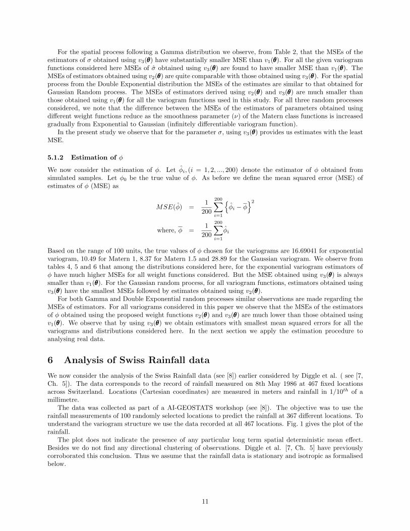
We now consider the analysis of the Swiss Rainfall data (see [8]) earlier considered by Diggle et al. ( see [7,Ch. 5]). The data corresponds to the record of rainfall measured on 8th May 1986 at 467 fixed locationsacross Switzerland. Locations (Cartesian coordinates) are measured in meters and rainfall in 1/10th of amillimetre.

The data was collected as part of a AI-GEOSTATS workshop (see [8]). The objective was to use therainfall measurements of 100 randomly selected locations to predict the rainfall at 367 different locations. Tounderstand the variogram structure we use the data recorded at all 467 locations. Fig. 1 gives the plot of therainfall.

The plot does not indicate the presence of any particular long term spatial deterministic mean effect.Besides we do not find any directional clustering of observations. Diggle et al. [7, Ch. 5] have previouslycorroborated this conclusion. Thus we assume that the rainfall data is stationary and isotropic as formalisedbelow.

11

Figure 1: Swiss Rainfall Plot. The figure shows the rainfall received at a particular geographical locationin Switzerland. The radii of the circles are proportional to the amount of rainfall. Figure reproduced fromDiggle et al.[7]

Let Y (si), denote the rainfall recorded at location si. Since the mean of the process does not depend onlocations we assume it satisfies the following model:

Y (si) = µ(si) + Z(si); i = 1, 2, ..., n, (25)

where µ(si) = E[Y (si)] = µ (constant). The vector of observations, Z(s) = Z(s1), Z(s2), ...Z(sn)′, follows a

multivariate distribution with 0 and dispersion Σ) such that Σ = [CovZ(si), Z(sj)]; (i, j) = 1, 2, ..., n. Z(si)is assumed to be a spatially second order stationary and isotropic process, so that Y (si) is also a second orderspatially stationary and isotropic. For computational simplicity we base our analysis on the mean deletedprocess Z(si) . We estimate the variogram parameters of some well known parametric functions, for therainfall data. The objective is to fit a suitable parametric variogram function to the sample variogram of theabove data.

As mentioned before, our principal focus is to predict the rainfall at 367 locations using the ’best’ vari-ogram; and in order to achieve this we need efficient criteria for the estimation of the underlying parametersof a suitably chosen variogram. We intend to acieve both these goals here.

For the sample variogram we plot in Fig 2 the classical variogram estimate, 2γ(h), calculated for 25different lag distances3 (‖h‖), where

‖h‖ = k.‖e‖; ‖e‖ = 10 units, k = 1, 2, ..., 25.

From Fig. 2 we observe that the sample variogram has some periodicity after the lag distance 50, increasinglinearly till then. Thus we consider a two parameter, sinusoidal, isotropic second order stationary variogramfunction to entertain the periodic nature of the rainfall data. In Geostatistical literature it is referred to ashole-effect or wave variogram (see e.g [16, p. 148]. The wave variogram is defined as follows

γ(‖h‖) = σ2 − σ2.(φ/‖h‖). sin(‖h‖/φ). (26)

We also consider the Matern class variogram functions, viz. Exponential, Matern 1, Matern 1.5 and Matern 2earlier used by Diggle et al.[7, Ch. 5] for this data. We have earlier (in (24)) defined the Matern Classvariogram.

3For the analysis reported here we have converted the Euclidean distance to Kilometre (KM) from metre.

12

Figure 2: Plot of Swiss Rainfall Sample Variogram.

For all the above parametric functions the unknown parameter vector is θθθ = (σ, φ)′.

We now present empirical analysis of the Swiss Rainfall in the following order.First, we provide and compare the results of estimation through the standard errors of estimates of the

unknown parameters. But as stated by Stein ([18]), among others, the parameter estimators of σ and φare correlated. In view of this we compare the joint variability using the measure Joint Standard Error(JSE) defined in (29) (see Appendix A). We also study the measure of deviation (goodness-of-fit) of thefitted curve from the sample variogram using the measure defined in (30) (see Appendix B). Finally, we usecross-validation kriging and the subsequent residual sum of squares, as defined in (32) to compare the effectof the estimates obtained by using the three different weight functions and the various variogram functionsin prediction (kriging).

Parameter Estimation The estimates of σ and φ and their standard errors for the Swiss rainfall dataare given in Table 7. We observe that the estimates of parameter σ “or sill” are much smaller (around 14percent) for the wave variogram than all the Matern class variogram functions considered. This indicatesthat for the Swiss rainfall data the Matern class variogram functions overestimate the variance of the randomprocess due to their non-periodic nature.

But more importantly, for both σ and φ the standard errors of the estimates are substantially lower forthe wave variogram compared to all other variogram functions considered. For σ the minimum standarderror of 1.03 is obtained using the weight function v3(θθθ) while the minimum standard error of estimate of φis 0.21 for v1(θθθ). But in view of the correlation of the estimates of σ and φ, we calculate JSE to study thejoint variability. The JSE is presented in Table 8. We denote the JSE corresponding to the weight functionvi(θθθ) by JSEi(θθθ); (i = 1, 2, 3) We note that the combined variance of estimates, JSE, of the wave variogramis also smaller than the Matern class variogram functions. Within the wave variogram, JSE of estimates ofσ and φ is minimum (1.02) for v3(θθθ) compared to 1.17 for v1(θθθ).

Goodness of fit Having estimated the parameters we now consider the goodness of the fit as aspects. InFigures 3 and 4 we give the plots of the fitted variograms corresponding to the respective weight functionsalong with the sample variogram, for comparison purposes. We note in Fig. 3 for the Matern class of

13

Figure 3: Variogram Fit- Rainfall Data. Each plot correspond to the respective variogram function used. Ineach plot three different curves, corresponding to the weights v1(θθθ), v2(θθθ) and v3(θθθ), are overlapped on thesample variogram.

Figure 4: Variogram Fit Plot -Wave Variogram. In the plot there are three curves overlapped on the samplevariogram plot which correspond to the weight functions v1(θθθ), v2(θθθ) and v3(θθθ)

variogram functions, that overall the plots of the estimated curves behave quite similarly; do not take intoaccount the periodic behaviour exhibited in the sample variogram; and result in overestimation of the samplevariogram.

A comparison of Fig. 4 with Fig. 3 reveals that there has been a significant improvement in the fit of thevariogram curve by using wave variogram as the parametric function. Table 9, given below, summarizes theabove observations.

14

Table 1: Goodness-of-Fit

Exponential Matern1 Matern 1.5 Matern 2 Wavev1(θθθ) 6382.617 5465.87 5334.34 5555.24 2752.401v2(θθθ) 6288.232 5472.62 5294.38 5238.38 2726.082v3(θθθ) 6406.145 5457.32 5307.59 5335.07 2698.278

From Table 9 we observe again that the wave variogram seems to give a better fit. We also note thatamong the weight functions, proposed earlier, v3(θθθ) has the minimum goodness-of-fit deviation (2698.28) forthe wave variogram.

Prediction We now consider if the above improvements can be seen in prediction. We calculate the residualsum of squares of cross validation kriging as defined in (32) (see Appendix C, see also [5, Ch. 2]). This allowsus to compare the performance of the variogram functions as well as the weight functions. We summarizethe results in the following table.

The above analysis using a non-parametric variogram estimation technique (also called curve fitting)makes it clear that the Matern class of variograms can not properly explain the underlying sample variogramof the present Swiss Rainfall data.

The residual prediction sums-of-squares are smaller for the wave variogram, compared to all other vari-ogram functions considered. Based on the above analyses we believe that for the Swiss Rainfall data and forother spatial processes which exhibit periodic sample variogram, the wave variogram is appropriate.

The minimum value of residual sum of squares is 0.1569 observed for v3(θθθ) as the weight function. Theresidual sum of squares of prediction, obtained for the wave variogram using the weight function v1(θθθ) ishigher than those obtained using the proposed weights v2(θθθ) and v3(θθθ). The above tables provide clearempirical evidence that estimation using the proposed weight functions v2(θθθ) and v3(θθθ) results in betterprediction results, when we use weighted least squares for estimation.

It should be noted here that the rainfall data has previously been analysed by other techniques such asmaximum likelihood estimation, in particular, after non-linear transformation of the original data (see e.g[7, Ch 5]). But as noted by Das [6] it leads to higher residual sums-of-squres for kriging, irrespective of thevariogram function and weight criterion used. We re-emphasize that the analyses we carried out are on theoriginal observations.

7 Conclusions

In this article we have introduced two alternative weight functions (v2(θθθ) and v3(θθθ)) as improvements to thewidely used weight function v1(θθθ) for parametric variogram estimation using weighted least squares method.Under the ’mixed increasing domain’ sampling design proposed in [11] we have established that asymptoticvariance of the parameter estimators obtained using v3(θθθ) is smaller than that obtained using v1(θθθ). We haveprovided empirical evidence using descriptive methods which demonstrate that for an appropriate choice ofvariogram function, estimation using v2(θθθ) and v3(θθθ) lead to better prediction and estimation results. We havealso seen empirical evidence that for Matern class functions increasing the smoothness parameter shifts thefitted curves more towards the extreme sample variogram values. This leads to a misleading goodness-of-fitmeasure in the process.

We have also proposed the wave variogram as an alternative way to model the variogram properties ofthe widely used Swiss rainfall data and conclude that the proposed variogram gives better predictions atunknown locations.

8 Acknowledgements

The work presented in this article was pursued at the University of Manchester, with sponsorship from BritishCouncil under the UKIERI research grant and the first author received additional funds from Departmentof Science and Technology, as a Research Associate at the C.R.Rao AIMSCS, for preparing the article. Theauthors would like to thank Dr. Peter Neal of University of Manchester, Prof. Peter Diggle of University of

15

Lancaster and Dr. Suhasini Subbarao of Texas AM University for many useful suggestions that helped toimprove the article.

References

[1] Douglas M. Bates and S. DebRoy. Nonlinear Least Squares. Website, 1999. http://sekhon.berkeley.edu/stats/html/nls.html.

[2] P. Billingsley. Probability and Measure, 1995. John Wiley & Sons.

[3] P.J. Brockwell and R.A. Davis. Time series: theory and methods. Springer, 1991.

[4] N. Cressie. Fitting variogram models by weighted least squares. Mathematical geology, 17(5):563–586,1985.

[5] N.A.C. Cressie. Statistics for spatial data. John Wiley & Sons, New York, 1993.

[6] S. Das. Statistical Estimation of Variogram and Covariance Parameters of Spatial and Spatio-TemporalRandom Processes. PhD thesis, School of Mathematics, 2011.

[7] P.J. Diggle, J.A. Tawn, and R.A. Moyeed. Model-based geostatistics, volume 47. JSTOR, 1998.

[8] Gregoire Dubois. Spatial Interpolation Comparison. Website, 1997. https://wiki.52north.org/bin/view/AI_GEOSTATS/EventsSIC97.

[9] G. Hadley. Linear Algebra (Reading. 1961.

[10] Paulo J. Ribeiro Jr. and Peter Diggle. geoR: Analysis of Geostatistical Data. Website, 2009. http:

//cran.r-project.org/web/packages/geoR/index.html.

[11] S.N. Lahiri, Y. Lee, and N. Cressie. On asymptotic distribution and asymptotic efficiency of least squaresestimators of spatial variogram parameters. Journal of Statistical Planning and Inference, 103(1-2):65–85, 2002.

[12] B. Matern. Spatial variation. Springer-Verlag Berlin, 1986.

[13] G. Matheron. Principles of geostatistics. Economic geology, 58(8):1246, 1963.

[14] R Development Core Team. R: A Language and Environment for Statistical Computing. R Foundationfor Statistical Computing, Vienna, Austria, 2012. ISBN 3-900051-07-0.

[15] M. Rosenblatt. A central limit theorem and a strong mixing condition. Proceedings of the NationalAcademy of Sciences of the United States of America, 42(1):43, 1956.

[16] O. Schabenberger and C.A. Gotway. Statistical methods for spatial data analysis. CRC Press, 2005.

[17] M. Sherman and E. Carlstein. Nonparametric estimation of the moments of a general statistic computedfrom spatial data. Journal of the American Statistical Association, 89(426):496–500, 1994.

[18] M.L. Stein. Interpolation of Spatial Data: some theory for kriging. Springer Verlag, 1999.

[19] D.L. Zimmerman and M.B. Zimmerman. A comparison of spatial semivariogram estimators and corre-sponding ordinary kriging predictors. Technometrics, 33(1):77–91, 1991.

16

Table 2: Sampling Properties of σ (Gaussian Random Process)v1(θ)θ)θ) v2(θ)θ)θ) v3(θ)θ)θ)

Variogram Mean MSE Bias Mean MSE Bias Mean MSE BiasExponential 4.55 1.24 0.08 4.42 0.86 -0.05 4.44 0.70 -0.03Matern 1 4.46 0.74 -0.02 4.32 0.54 -0.16 4.36 0.49 -0.12Matern 1.5 4.44 0.75 -0.04 4.29 0.54 -0.18 4.33 0.50 -0.14Gaussian 4.39 1.70 -0.08 4.24 1.58 -0.23 4.30 1.53 -0.17

Table 3: Sampling Properties of σ (Gamma Random Process)v1(θ)θ)θ) v2(θ)θ)θ) v3(θ)θ)θ)

Variogram Mean MSE Bias Mean MSE Bias Mean MSE BiasExponential 4.45 1.42 -0.03 4.32 1.18 -0.15 4.36 1.03 -0.11Matern 1 4.34 0.95 -0.13 4.21 0.85 -0.27 4.27 0.85 -0.20Matern 1.5 4.32 0.98 -0.15 4.18 0.88 -0.30 4.25 0.89 -0.23Gaussian 4.18 1.80 -0.29 4.05 1.74 -0.42 4.13 1.75 -0.35

Table 4: Sampling Properties of σ (Double Exponential Random Process)v1(θ)θ)θ) v2(θ)θ)θ) v3(θ)θ)θ)

Variogram Mean MSE Bias Mean MSE Bias Mean MSE BiasExponential 4.58 1.42 0.11 4.46 1.02 -0.01 4.47 0.91 0.00Matern 1 4.51 1.04 0.04 4.35 0.79 -0.12 4.40 0.80 -0.07Matern 1.5 4.50 1.02 0.02 4.33 0.81 -0.14 4.39 0.84 -0.08Gaussian 4.39 1.90 -0.08 4.27 1.82 -0.20 4.32 1.77 -0.15

Table 5: Sampling properties of estimates of φ ( Gaussian Random Process)v1(θ)θ)θ) v2(θ)θ)θ) v3(θ)θ)θ)

Variogram Mean MSE Bias Mean MSE Bias Mean MSE BiasExponential 22.03 616.00 5.34 20.12 281.93 3.43 18.91 167.12 2.21Matern 1 11.94 50.00 1.45 10.95 20.43 0.46 10.64 13.19 0.15Matern 1.5 9.36 26.11 0.99 8.53 9.41 0.16 8.32 5.77 -0.05Gaussian 29.71 119.94 0.82 28.91 110.63 0.02 28.63 84.47 -0.26

Table 6: Sampling properties of estimates of φ (Gamma Random Process)v1(θ)θ)θ) v2(θ)θ)θ) v3(θ)θ)θ)

Variogram Mean MSE Bias Mean MSE Bias Mean MSE BiasExponential 20.22 721.69 3.53 19.46 334.54 2.77 17.93 170.44 1.24Matern 1 11.03 33.74 0.54 10.65 21.35 0.16 10.28 14.00 -0.21Matern 1.5 8.71 16.33 0.34 8.32 9.13 -0.05 8.09 6.10 -0.28Gaussian 28.01 62.67 -0.88 27.37 86.92 -1.52 27.62 62.72 -1.27

Table 7: Sampling properties of estimates of φ (Double Exponential Random Process)v1(θ)θ)θ) v2(θ)θ)θ) v3(θ)θ)θ)

Variogram Mean MSE Bias Mean MSE Bias Mean MSE BiasExponential 22.05 757.13 5.36 21.27 321.70 4.58 19.07 136.24 2.38Matern 1 12.24 69.72 1.75 11.26 22.05 0.77 10.77 13.89 0.28Matern 1.5 9.54 30.45 1.17 8.69 9.32 0.32 8.43 6.08 0.06Gaussian 28.76 112.70 -0.13 28.29 174.05 -0.60 28.31 75.46 -0.57

17

Table 8: Estimates and Standard Errors of Variogram Parameters

v1(θθθ) v2(θθθ) v3(θθθ)

Variogram function Statistic σ φ σ φ σ φExponential estimate 118.729 34.072 117.767 33.74 118.754 35.298

stderr (2.094) (4.189) (1.996) (4.157) (2.163) (4.183)Matern1 estimate 117.336 19.482 116.638 19.49 117.072 19.525

stderr (1.48) (1.347) (1.441) (1.574) (1.473) (1.368)Matern1.5 estimate 116.56 14.154 116.309 14.928 116.42 14.3682

stderr (1.4692) (0.8946) (1.355) (1.08) (1.4361) (0.9235)Matern2 estimate 115.711 11.1104 116.158 12.5408 116.09 11.758

stderr (1.7342) (0.6432) (1.3344) (0.8679) (1.469) (0.749)Wave estimate 103.7291 17.6437 102.7444 17.6592 103.1531 17.6269

stderr (1.0933) (0.2126) (1.1206) (0.2248) (1.0312) (0.2472)

Table 9: Joint Standard Error for σ and φ

JSE1(θθθ) JSE2(θθθ) JSE3(θθθ)Exponential 5.88 5.73 5.95

Matern-1 2.51 2.66 2.52Matern-1.5 2.07 2.11 2.06

Matern-2 2.14 1.91 1.94Wave 1.17 1.19 1.03

Table 10: Goodness-of-Fit

Exponential Matern1 Matern 1.5 Matern 2 Wavev1(θθθ) 6382.617 5465.87 5334.34 5555.24 2752.401v2(θθθ) 6288.232 5472.62 5294.38 5238.38 2726.082v3(θθθ) 6406.145 5457.32 5307.59 5335.07 2698.278

Table 11: Kriging Residual Sum of Squares- Original data Wave Variogram

Exponential Matern1 Matern 1.5 Matern 2 Wavev1(θθθ) 0.570166 2.61485 8.98134 20.0277 0.17036v2(θθθ) 0.575658 2.6305 9.00066 19.9505 0.157217v3(θθθ) 0.570873 2.62075 8.99209 19.9623 0.156936

A Asymptotic Unbiasedness of the estimating equation for Pro-posed Criterion Q3n(θθθ)

We have earlier pointed out that v1i(θθθ) leads to biased generalized estimating equations. We show belowthat using v3i(θθθ) we obtain an approximately unbiased generalized estimating equation. We note that differ-entiating Q3n(θθθ) with respect to each element of θθθ, we have for each j,

∂Q3n(θθθ)

∂θj=

k∑i=1

[ln 2γ(hi)− ln 2γ(hi, θθθ)]∂ ln 2γ(hi, θθθ)

∂θj

|N(hi)|2

j = 1, 2, ..., p

18

hence,

E[∂Q3n(θθθ)

∂θj] w 0 since, approximately

E[ln 2γ(hi)] ' ln 2γ(hi, θθθ) (27)

Thus, use of v3i(θθθ) makes the generalized estimating equations approximately unbiased.

B Definitions and Notations for Asymptotic normality

g(θθθ) =

2γ(h1)− 2γ(h1, θθθ)2γ(h2)− 2γ(h2, θθθ)

.

.

.2γ(hk)− 2γ(hK , θθθ)

(K×1)

The vector of first derivatives

∇lg(θθθ) =∂

∂θlg(θθθ) =

−2 ∂∂θlγ(h1, θθθ)

−2 ∂∂θlγ(h2, θθθ)

.

.

.−2 ∂

∂θlγ(hK , θθθ)

=

−2γl(h1, θθθ)−2γl(h2, θθθ)

.

.

.−2γl(hK , θθθ)

where ∇lγ(h, θθθ) = ∂γ(h,θθθ)

∂θlfor l = 1, 2, ..., q, Let us define the matrix of first derivatives as

D(θθθ) = [g1(θθθ),g2(θθθ), ...,gq(θθθ)](K×q)

∇lg3(θθθ) =∂

∂θlg3(θθθ)

=

− ∂∂θl

ln 2γ(h1, θθθ)

− ∂∂θl

ln 2γ(h2, θθθ)

.

.

.− ∂∂θl

ln 2γ(hk, θθθ)

=

− 12γ(h1,θθθ)

2 ∂∂θlγ(h1, θθθ)

− 12γ(h2,θθθ)

2 ∂∂θlγ(h2, θθθ)

.

.

.− 1

2γ(hK ,θθθ)2 ∂∂θlγ(hK , θθθ)

D3(θθθ) = [g31(θθθ),g32(θθθ), ...,g3q(θθθ)](K×q)

V1(θθθ) = [Σ−11 (θθθ)]

(28)

C Choice of Initial Values for parameters

The package needs initial values of the parameters as seed values for the first iteration. In the next steps wedescribe the method for choosing initial values of parameters. Let the initial values be denoted by σ∗ andφ∗.

19

• For a sample from a given distribution (e.g Gaussian) 200 samples of spatial random processes, of size100 each, is generated. Variograms are computed at each of the lags (here we have chosen 20 lags).Thus, we have a set of 200 sample variograms each computed for 20 different euclidean lag distances.Then, we compute an average sample variogram over all the lags by computing an arithmetic meanover all the 200 sample variograms.

• Since, the theoretical variogram 2γ(h, θθθ) → σ2 (the variance of the process), as ‖h‖ → ∞, the squareroot of the mean sample variogram, at the maximum lag distance, is used as the initial parameter valuefor σ. We may denote this by σ∗.

• From our discussions in Chapter 1 we know practical range is the lag distance h+ for which we haveγ(h+, θθθ) = 0.95σ2. Using the starting value σ∗ we now find the practical range h+ for the variogramfunctions considered from the sample variograms computed.

• Then the starting value φ∗ is obtained by solving the following non-linear equation.

γ(h+, θθθ) = 0.95σ∗2

where θθθ = (σ∗, φ∗)

• With the estimates available for both parameters for each of the 200 samples we compute the mean,bias and mean squared errors (MSE) for each parameter over the 200 sets. Then the estimates arecompared.

D Descriptive Measures for Data Analysis

Standard Error and Joint Variability It is well known that the Matern class variogram parametersare correlated (see e.g [18]) To assess the combined variability of correlated parameter estimates of σ and φone could use many standard techniques for instance, determinant of the information matrix or eigenvaluesof the variance covariance matrix etc. Here we will consider the following simple measure of joint variability

Joint Standard Error(JSE) =

√se(σ)2 + se(φ)2 + 2 Covσ, φ (29)

Goodness-of-Fit/Deviation Measure The parameter variability is followed by an assessment of the fit.We analyze the fit using the following measure. The fit of the sample variogram of the data to the theoreticalfunctions over k lag distances is considered to be good if the following deviation measure is low.(1/k)

k∑j=1

(γ(hj)− γ(hj))21/2

. (30)

Cross validation : After finding the ’best’ function, once again it would be useful to check its performancein ’prediction’ at unobserved locations, using the kriging methodology, described in Chapter 1. One way ofassessing the goodness of the fitted variogram is to use the cross-validation method. Where we omit oneobservation at any location and use the other locations for predicting it. We use the technique discussed inCressie ([5, pg.102]). Given below are the details of the method. Briefly we describe the steps. The processinvolves three steps:

1. We estimate and plot the sample variogram 2γ(h) as a function of the k lag distances ‖hi‖, i = 1, 2, ..., kusing the entire sample of the random process from all the locations.

2. Once we have decided on a suitable theoretical variogram -using the methods described above- we useit to predict the random process at various locations, omitting the observation at jth location and usingthe rest of the available locations to predict the value at this location, using kriging. We denote sucha predictor by Z((s)−j) and the associated standard error of prediction by σ−j((s)j).

20

3. We plot histograms of the residuals of prediction, which we define as follows:(Z((s)j)− Z((s)−j)

)/σ−j((s)j)

. (31)

As a single approximate measure we compute the sum of the squares of residuals to measure thegoodness of fit of prediction.[

(1/n)

n∑i=1

(Z(sj)− Z(s−j)

)/σ−j((s)j)

2]1/2

. (32)

Though not much is known about the theoretical statistical properties of the above residual and the sum ofsquares, we should expect the histogram of a good predictor to be ’closely’ distributed about the mean zero.And the sum of squares should be small.

21