On the Effectiveness of Single and Multiple Base Station Sleep Modes

in Cellular Networks ✩

Marco Ajmone Marsana,b , Luca Chiaraviglioc , Delia Ciullod , Michela Meoa

a) Electronics and Telecommunications Department, Politecnico di Torino, Italyb) Institute IMDEA Networks, Madrid, Spain

c) University of Rome La Sapienza, Italyd) EURECOM Sophia-Antipolis, France

Abstract

In this paper we study base station sleep modes that, by reducing power consumption in periods of low traffic,improve the energy efficiency of cellular access networks. We assume that when some base stations enter sleep mode,radio coverage and service provisioning are provided by the base stations that remain active, so as to guarantee thatservice is available over the whole area at all times. This may be an optimistic assumption in the case of the sparse basestation layouts typical of rural areas, but is, on the contrary, a realistic hypothesis for the dense layouts of urban areas,which consume most of the network energy.We consider the possibility of either just one sleep mode scheme per day (bringing the network from a high-power,

fully-operational configuration, to a low-power reduced configuration), or several sleep mode schemes per day, withprogressively fewer active base stations. For both contexts, we develop a simple analytical framework to identify optimalbase station sleep times as a function of the daily traffic pattern.

We start by considering homogeneous networks, in which all cells carry the same amount of traffic and cover areasof equal size. Considering both synthetic traffic patterns and real traffic traces, collected from cells of an operationalnetwork, we show that the energy saving achieved with base station sleep modes can be quite significant, the actualvalue strongly depending on the traffic pattern. Our results also show that most of the energy saving is already achievedwith one sleep mode scheme per day. Some additional saving can be achieved with multiple sleep mode schemes, at theprice of a significant increase in complexity.We then consider heterogeneous networks in which cells with different coverage areas and different amounts of traffic

coexist. In particular, we focus on the common case in which some micro-cells provide additional capacity in a regioncovered by an umbrella macro-cell, and we prove that the optimal scheduling of micro-cell sleep times is in increasingorder of load, from the least loaded to the most loaded. This provides a valuable guideline for the scheduling of sleepmodes (i.e., of low-power configurations) in complex heterogeneous networks.

Keywords: Energy-efficiency, Cellular networks, QoS and sleep modes

1. Introduction

Eskimos are said to use many words for snow, becausesnow pervades their environment. On the contrary, in theearly days of networking, the term power was used to iden-tify the ratio of throughput over delay [3, 4], because en-ergy issues did not belong in the networking landscape.Then, cellular networks and battery-operated terminals

✩Some of the results in this paper have been presented in [1] and[2].

∗Corresponding Author: Delia Ciullo, EURECOM Sophia-Antipolis, France. Email: delia.ciullo@eurecom.fr, tel. +33-0493008280.

Email addresses: ajmone@polito.it ( Marco AjmoneMarsana,b ), luca.chiaraviglio@diet.uniroma1.it ( LucaChiaraviglioc ), delia.ciullo@eurecom.fr ( Delia Ciullod ),michela.meo@polito.it ( Michela Meoa )

(most notably mobile phones) came along, and power con-trol (now real power, measured in J/s) became an issue,in order to extend both the distance from the base sta-tion at which a terminal could be used, and the batterycharge duration (in the early ’90s, heavy users carried aspare charged battery in their pocket, to avoid being cut offaround noon). Next, sensor networks brought with themthe question of power minimization to increase the net-work lifetime. Still, before the turn of the century, powerconsumption was not an element of the wired network de-sign space. The first paper that addressed energy issuesin fixed networks was [5], where Gupta and Singh inves-tigated the energy consumption of Internet devices, anddiscussed the impact of sleep modes on network proto-cols. Since then, the interest in energy-efficient networkinghas been steadily rising, and the energy issue is now ad-

Preprint submitted to Computer Networks July 18, 2013

dressed in many conferences and research projects, amongwhich we wish to mention TREND (Towards Real Energy-efficient Network Design) [6], the Network of Excellencefunded by the European Commission within its 7th Frame-work Programme, which supported the work reported inthis paper.The directions that are presently pursued to achieve

energy efficiency in networking can be grouped in twoclasses: 1) development of new technologies that reduceenergy consumption, and 2) identification of approachesthat make the network energy consumption proportionalto traffic. The rationale for the second direction derivesfrom the observation that today network equipment ex-hibits power consumption which is practically independentof load. For example, a base station of a cellular networkconsumes at zero load about 60-80% of the energy con-sumption at full load [7].Approaches that aim at improving the proportionality

between the network energy consumption and the networkload can be further divided in 2 sub-classes: 2a) devel-opment of equipment exhibiting better proportionality ofenergy consumption to load, and 2b) identification of algo-rithms that allow the reduction of the functionality of net-work equipment in periods of low traffic, so as to decreaseenergy consumption in such periods. The algorithms thatreceived most attention in class 2b are often called speedscaling, and s leep modes. By speed scaling we normallymean that the equipment can operate at different clockrates, with lower rates corresponding to lower power (andlower performance). By sleep modes we mean that in pe-riods of low traffic the network operates with a subset ofits equipment, the rest being switched off to save energy.In the case of cellular networks, the critical equipment

for power consumption is the base station (BS), whosetypical consumption ranges between 0.5 kW and 2 kW[8, 9], including power amplifiers, digital signal processors,feeders, and cooling system. Moreover, according to [10],all together, the BSs make up for about 80% of the totalenergy consumption of the cellular network.In this paper we consider sleep modes for BSs in cel-

lular networks, with reference to 3G technology, and weinvestigate the benefits that can be achieved by puttingto sleep, i.e., bringing to a low-power-idle (LPI) state, aBS during periods of low traffic. This means that, in thefuture, the cellular access network planning should allowthe selection of different operational layers correspondingto network configurations that specify the set of active BSsto serve different levels of traffic. These configurationscan be activated according to predefined schedules, thatare derived based on a combination of traffic forecasts andlogs of traffic measurements. We compute the maximumamount of energy that can be saved with this approach,and we study the impact of the number of configurations,considering different types of network topologies with ide-alized cell structures. We then consider a real BS layoutin a urban environment and a realistic coverage map, andshow that significant savings can be achieved also in this

scenario.We assume that when some BSs are in sleep mode, radio

coverage and service provisioning are taken care of by thebase stations that remain active, so as to guarantee thatservice is available over the whole area at all times. Thismay be an optimistic assumption in the case of sparsebase station layouts in rural areas (where network plan-ning usually aims at coverage using large cells), but is onthe contrary a realistic hypothesis for the dense layouts ofurban areas (where network planning normally aims at ca-pacity, with very redundant coverage, based on few largeand many small cells), which consume most of the networkenergy. When some BSs enter the LPI state, the base sta-tions that remain active may need to increase their trans-mission power, so as to cover also the area that was coveredby the sleeping BSs. However, in our previous study [18]we showed that this increment in power consumption isusually negligible.The main contributions of this paper are the following.

We develop an analytical framework to identify the opti-mal scheduling of low-power network configurations (in-cluding how many BSs should be put into sleep mode andwhen) as a function of the daily traffic pattern, in the casesin which either just one low-power configuration per dayis possible (bringing the network from a high-power, fully-operational configuration, to a low-power reduced-capacityconfiguration), or several low-power configurations per dayare permitted (progressively reducing the number of ac-tive base stations, the network capacity, and the networkpower). We then compute the achievable energy savingsin several cases: i) assuming that any fraction of base sta-tions can be put to sleep, ii) accounting for the constraintsresulting from typical regular base station layouts, and iii)considering the case of a realistic network deployment inthe city center of Munich. Moreover, we consider het-erogeneous networks in which coverage is obtained by thesuperposition of macro-cells, that act as umbrella cells,and micro-cells, that provide additional capacity in spe-cific areas. We prove that the optimal scheduling accord-ing to which micro-cells should be put to sleep is in orderof increasing load. We show that, in a realistic heteroge-neous network with real traffic profiles, large savings canbe achieved by putting BSs to sleep, starting from the leastloaded to the most loaded.The rest of the paper is organized as follows. Section

2 reviews the related literature. Optimal energy savingsschemes for homogeneous networks are presented in Sec-tion 3. Savings on regular configurations are computed inSection 3.5. Section 4 details the analysis of heterogeneousnetworks, and provides a case study of a real network. Sec-tion 5 discusses implementation issues. Finally, Section 6concludes the paper.

2. Related Work

The fact that BSs are the most energy-greedy compo-nents of cellular networks, and are often under-utilized,

2

was realized only few years ago [10, 11, 12, 13]. Sincethen, several approaches have been pursued to reduce thecarbon footprint of BSs, ranging from the use of renewableenergy sources [14], to the improvement of hardware com-ponents [15], to cell zooming techniques [16], to the adop-tion of sleep modes. As regards to sleep modes, startingfrom our early works [17, 1, 18], it has been shown thatsleep modes adoption for BSs is an efficient solution thatallows a significant amount of energy to be saved duringlow traffic periods. Later, also the authors of [19] showed,using real data traces, that promising potential savingsare achievable by turning off BSs during low traffic peri-ods. Recently, in [20] the authors have investigated energysavings in dynamic BS operation and the related problemof user association, showing that their algorithms can sig-nificantly reduce the energy consumption. A distributedsolution to switch off underutilized BSs when traffic is low,and switch them on when traffic is high, was proposed in[21]; large savings, that depend on temporal-spatial trafficdynamics, are shown to be possible.

Besides BSs switch-off, sleep modes can be enabled alsoconsidering different options, ranging from the reduction ofthe number of active transmitters [22], to the switch-off ofa whole network, when coverage is provided by other tech-nologies of the same operator, or when several operatorsoffer coverage in the same service area [23], by allowingcustomers to roam from the network that switches off toone that remains on.

Differently from most previous works, but expandingour analysis in [1] and [2], here we analytically character-ize the maximum energy savings that can be achieved inregular networks, under a given traffic profile. In partic-ular, we analytically show that the optimal trade-off be-tween energy savings and complexity in network manage-ment is obtained when only few low-power configurationsper day are allowed, and BSs are put to sleep according toincreasing load. These results are also corroborated by acase-study analysis.

The extensions that we provide with respect to [1] and[2] are mainly the following: i) we consider a more real-istic energy consumption model; ii) we consider the caseof multiple, progressive low-power configurations per day,proving that small numbers of configurations are sufficientto achieve most of the possible energy savings; iii) we provethat the optimal sleep order consists in putting BSs tosleep in increasing order of load; iv) we consider differentcell types (business and residential); v) we obtain analyt-ical results from a more detailed synthetic traffic pattern;and vi) we consider as a case study the heterogeneous BSlayout in a square of 800 by 800 m in downtown Munich,with real traffic profiles, resulting from measurements inan operational network.

T/2 t

1

f(τ1)

τ1

f(τ3)

τ3

Saving

f(τ2)

τ2

Figure 1: Example of multiple sleep schemes with N =3.

3. Optimal Sleep Modes in Homogeneous Net-

works

In this section we propose a simple analytical frame-work to compute the maximum energy saving that can beachieved by properly scheduling multiple low-power net-work configurations in homogeneous networks. We firstconsider an idealized synthetic traffic profile, that we calltwo-step traffic pattern, for which we easily obtain analyt-ical results. Then, we present results obtained with somemeasured traffic patterns collected from a cellular networkin operation.

3.1. The network and traffic model

Let f(t) be the daily traffic pattern in a cell, i.e., thetraffic intensity as a function of time t, with t ∈ [0, T ],T = 24 h, and t = 0 at the peak hour; f(t) is normalizedto the peak hour traffic, so that f(0) = 1. As an example,in Fig. 1 we report a typical daily traffic pattern that, forsimplicity, is symmetric around T/2. We assume that f(t)is a continuous and differentiable function of t.

The cellular access network is dimensioned so that atpeak traffic a given QoS constraint is met. Clearly, if theQoS constraint is met under peak traffic f(0), it is alsomet for lower values of traffic intensity, and thus duringthe whole day. For analytical tractability, we assume thatin the considered area all cells have identical traffic pat-terns; thus, we say that the network is homogeneous. Werecognize that BSs deployed in real networks can be sub-jected to different traffic patterns, and we will considertraffic heterogeneity in Section 4.

Consider an area with M homogeneous cells and con-sider a low-power network configuration Φ such that, dur-ing periods of low traffic, a fraction x < 1 of the cells, i.e.,xM cells, are active, while the remaining fraction, 1 − x,of the cells (actually, of the respective BSs) are in LPI(or sleep) mode. When the low-power configuration Φ isapplied, the xM active BSs have to collectively sustain,in addition to their own traffic, the traffic that in normalconditions is taken care of by the (1− x)M sleeping BSs;thus, their traffic becomes:

f (Φ)(t) = f(t) +(1− x)M

xMf(t) =

1

xf(t) (1)

3

i.e., an active cell receives 1/x times its own traffic1. Thus,to always satisfy the QoS constraint, Φ can be appliedwhenever the traffic f(t) is so low that f (Φ)(t) is still below1, that is the peak hour traffic; this is what we call the loadconstraint,

f (Φ)(t) =1

xf(t) < 1 (2)

Starting from the peak hour, with decreasing f(t), theearliest time instant τ in which Φ can be applied is definedby,

f (Φ)(τ) = 1 (3)

so that,τ = f−1(x) (4)

By assuming that the low-power configuration Φ is appliedas soon as the traffic profile permits, the scheme Φ is fullyspecified by the value of τ . Considering, for simplicity, adaily traffic pattern that is symmetric around T/2, i.e.,such that f(τ) = f(T −τ) with τ ∈ [0, T/2], and assumingthat f(t) is monotonically decreasing in [0, T/2], the periodin which Φ can be applied starts in τ and lasts for the wholetime in which the traffic intensity is below f(τ) = x, i.e.,for a period of duration T − 2τ .

3.2. The energy consumption model

Coherently with the assumption of a homogeneous net-work, we assume that in the considered area all BSs haveidentical power consumption. Actually, BSs deployed inreal networks may consume a different amount of power(e.g., due to different technology); however, the assump-tion that all the BSs consume the same amount of power isreasonable, at least in some portions of dense urban areas.For each BS, we assume that the power consumption

equals WLPI in the LPI state, i.e., when the BS is in sleepmode. Instead, when the BS carries a traffic f(t), its powerconsumption can be expressed as

P (t) = WLPI +W0 +WT f(t) (5)

where W0 is the power necessary for an active BS carryingzero traffic, in addition to WLPI , and WT is the powernecessary for the BS to handle one unit of traffic. Notethat, in our computations, we will consider the normalizedvalues of the three power components, such that the sumis equal to one when the traffic is maximum (i.e., equal toone).Obviously, the values of WLPI , W0, and WT depend on

the BS technology and model, but normally the W0 com-ponent dominates (for numerical values see for example[9], [24]). Typically, the higher is the power consumptionin the LPI state, the shorter is the BS activation time.Therefore, the values of WLPI depend on the policy that

1Note that (1) holds for the case of a specific low-power networkconfiguration, Φ, in an area where M cells are deployed. Whenseveral low-power configurations are used, the condition of (1) musthold for each of them.

an operator may want to adopt, based on activation anddeactivation times of BSs. In our computations, we willuse low values of WLPI , since we assume the BSs are putin LPI state only few times per day. This implies that ac-tivation/deactivation times, even if long in absolute terms(e.g., tens of seconds or even few minutes), can be consid-ered negligible with respect to long sleep time intervals.The energy consumed in a day by a BS in a cellular

network in which all BSs remain always on is

EALLON =∫ T

0(WLPI +W0 +WT f(t)) dt

= T (WLPI +W0) +WT

∫ T

0f(t)dt

(6)

Consider now a network in which the low-power config-uration Φ is applied at time τ . In this case, the BSs havedifferent daily consumption, depending on whether theyare always on or they enter sleep mode when traffic is low.The energy consumed in a day by a BS which is put tosleep according to configuration Φ is equal to

ESLEEP = 2∫ τ

0(WLPI +W0 +WT f(t)) dt

+ 2(T/2− τ)WLPI

= TWLPI + 2τW0 + 2WT

∫ τ

0f(t)dt

(7)

because from 0 to τ and from T − τ to T the BS is on,while for the rest of the day the BS is in the LPI state. Theenergy consumed in a day by a BS which remains on whileother cells are put to sleep according to configuration Φ isequal to

EON = 2∫ τ

0(WLPI +W0 +WT f(t))dt

+ 2∫ T/2

τ(WLPI +W0 +WT

1xf(t))dt

= T (WLPI +W0) + 2WT

∫ τ

0f(t)dt

+ 2WT1x

∫ T/2

τf(t)dt

(8)

because from 0 to τ and from T − τ to T the BS carriesonly its traffic share, while for the rest of the day the BScarries also a portion of the traffic of the BSs in the LPIstate.Considering that a fraction 1 − x of the BSs is put to

sleep according to configuration Φ, while the remainingfraction x remains on, the average energy consumption ofa BS is

EΦ = (1− x)ESLEEP + xEON

= TWLPI + [2(1− x)τ + Tx]W0

+ 2WT

∫ τ

0f(t)dt+ 2xWT

1x

∫ T/2

τf(t)dt

= TWLPI + TW0 − (1− x)[T − 2τ ]W0

+ WT

∫ T

0f(t)dt

(9)

Thus, the energy saved by using configuration Φ withrespect to the always-on case is:

S = EALLON − EΦ = (1− x)[T − 2τ ]W0 (10)

which corresponds to saving the power W0 for the fractionof cells in LPI state, and for the period in which the low-power configuration Φ is used. The fact that no traffic is

4

lost is reflected in the independence of S from WT . In thenumerical results that we will report in what follows wewill often use the percentage saving obtained by dividingS by EALLON .

Let us now focus on the case of multiple low-power con-

figurations in which N low-power network configurationsare allowed per day, each configuration being denoted byΦi with i = 1, ..., N . In particular, given a decreasing traf-fic profile f(t), symmetric around T/2, we assume thatthe configurations Φi are ordered in such a way that thefraction of BSs in sleep mode increases with i. In otherwords, we assume to put to sleep a fraction (1−x1) of BSsat a certain time instant τ1, a fraction (1 − xi) at τi, ...,and (1 − xN ) at τN , with x1 > · · · > xi > · · · > xN . Letthe N−dimensional vector τ collect the switching instantsτi, i.e., τ = [τ1, τ2, · · · , τN ]. Extending (10), the energysaving with respect to the always-on case is,

SN (τ) = 2W0

N∑

i=1

(τi+1 − τi)(1− f(τi)) (11)

with τN+1 = T/2. Indeed, with reference to Fig. 1 for thecase N = 3, the saving is given by the white area made ofthree rectangles and, for example, from τ1 to τ2 the savingis given by 1 − f(τ1)(τ2 − τ1), from τ2 to τ3 the saving isgiven by 1− f(τ2)(τ3 − τ2), and so on.

The saving can be maximized (and the consumptionminimized) by choosing the configurations Φi so as tomaximize SN (τ). Assuming that the function SN (τ) ispiecewise differentiable and convex (these conditions aresatisfied by construction given the conditions we imposedon f(τ)), the optimal choice of the schemes, i.e., the op-timal τ , namely τ∗, is such that ∂SN (τ)/∂τi = 0, fori = 1, · · · , N . The optimal scheme is given by the solutionof the following system of equations,

−f ′(τi)(τi+1 − τi) + f(τi)− f(τi−1) = 0, (12)

with i = 1, ..., N , and f ′(t) is the derivative of f(t) withrespect to time t, and τ0 = 0 (so that f(τ0) = 1) andτN+1 = T/2. Notice that there may exist different schemescorresponding to the same consumption, and there mayexist different solutions of (12) that are local maxima of(11); among these values, one of those leading to S(τ∗) canbe selected as the optimum. For example, in Fig. 2, two(single) low traffic configurations corresponding to timeinstants τ1 and τ2 lead to the same energy saving.

The corresponding maximum energy saving is denotedby SN and it represents the best that can be done un-der traffic f(t) by allowing the network to move across Ndifferent low-power configurations.

An upper bound to the achievable network saving canbe obtained by considering that the fraction of BSs thatis in sleep mode increases in a continuous way, throughinfinitesimal increments. In other terms, the upper boundof the saving, namely SU , can be computed as the com-

T/2 t

1

f(τ1)

τ1

f(τ2)

τ2

Saving1

Saving2

Figure 2: Two schemes achieving the same energy saving.

t

1

f(t)

T/2 T

L

L

LT/2

Figure 3: Synthetic traffic pattern.

plement of the integral of f(t),

SU = 2W02

T

∫ T/2

0

(1− f(τ))dτ (13)

In the case of a non-symmetric traffic pattern f(t), it canbe easily shown that the optimum scheme can be derivedin a similar way, by solving the derivative of the savingSN (τ) that corresponds to the asymmetric profile.

3.3. A synthetic traffic pattern

To start analyzing the effect of the number of networkconfigurations used in a day, we consider a synthetic trafficpattern, that, while being very simple, allows us to tunethe traffic shape by acting on a single scalar parameter.We consider the family of two-step traffic profiles plottedin Fig. 3 and defined by

f(t) =

L−1L

2tT + 1 0 ≤ t < T

2 L

LL−1 (

2tT − 1) T

2 L ≤ t ≤ T2

(14)

with L ∈ [0, 1]. The parameter L defines the position ofthe curve knee: the knee is in (LT/2, L); for L = 1/2the curve is made of just two segments: one for decreasingtraffic and one for increasing traffic. Note that lower valuesof L correspond to lower overall daily traffic loads.We start by analyzing the case of one low-power network

configuration, N = 1, that alternates to the normal full-capacity configuration. When L > 1/2, the maximumenergy saving is reached for two values of τ ,

τ∗ = T/23L− 1

2Land τ∗ = T/4 (15)

5

00.20.40.60.810

10

20

30

40

50

60

70

80

90

100

Parameter L

Sav

ing

[%]

Upper BoundN=3N=2N=1

Figure 4: Synthetic traffic pattern: maximum achievable saving forvarious number of network configurations versus the parameter L.

When L ≤ 1/2, the maximum occurs at the curve knee,that is for

τ∗ =TL

2(16)

When two low-power configurations are allowed, i.e., N =2, the maximum saving is achieved for (τ∗1 , τ

∗2 ) with,

(τ∗

1 , τ∗

2 ) =

{(

T4

L(3L−1)

2L2−1/2(L−1)2

, T2

L(3L−1)

2L2−1/2(L−1)2

)

if L > 1/3(

T2L, T

4(L+ 1)

)

otherwise(17)

For a case in which the BS consumption is independentof the traffic (similar to existing equipment), i.e., WT = 0in (5), Fig. 4 shows, in percentage, the maximum net-work saving versus L for various values of N ; the upperbound is also reported. Clearly, the saving increases withN , reaching the upper bound for N → ∞. Values of Nequal to 2 or 3 are enough to achieve saving that is closeto the upper bound. Higher values of N bring small addi-tional improvements only, while introducing higher com-plexity in network management. Indeed, larger values ofNmean more switching decisions (sleep mode entrance/exit)per day. This may lead to: i) higher instability in thesleep algorithms, due to the higher switching frequencies;ii) poorer quality of service caused by users’ disconnec-tion, due to frequent activation/deactivation of BSs. Bycomputing the difference between the maximum achiev-able saving in the case of two low-power configurationsand one only, we found that the saving increase is at most8%, suggesting that the use of two configurations insteadof one only does improve the maximum achievable saving,but to a limited extent.

3.4. Measured Traffic patterns

We now consider traffic profiles measured from the net-work of an anonymized cellular operator. In particular,we consider traffic profiles taken from two individual ur-ban cells with different user types: one cell refers to abusiness area, and the other one to an area that is mainlyresidential. Moreover, for each of these cells, we considertwo profiles: the weekday profile is chosen as the average of

0

0.2

0.4

0.6

0.8

1

00:00 05:00 10:00 15:00 20:00 00:00

Tra

ffic

, f(t

)

Time, t [h]

WeekdayWeekend

Figure 5: Business cell: weekday and weekend traffic profiles.

0

0.2

0.4

0.6

0.8

1

00:00 05:00 10:00 15:00 20:00 00:00

Tra

ffic

, f(t

)

Time, t [h]

WeekdayWeekend

Figure 6: Residential cell: weekday and weekend traffic profiles.

the weekday profiles collected during a week; the weekend

profile is an average of the two weekend days of the sameweek. The traffic profiles are reported in Figs. 5 and 6.Profiles are normalized to the weekday peak value, that oc-curs around 11am for the business area, and in the eveningfor the residential area. Clearly, two completely differenttrends characterize the two areas: traffic is concentratedduring the working hours of the weekdays for the businessarea, while traffic is higher during the evening for the res-idential area, where the difference between weekdays andweekends is marginal. However, for both profiles, trafficis very low from late night to early morning, i.e., from2.30am to 7.30am approximately. The transitions frompeak to off-peak and vice-versa are extremely steep in thebusiness weekday profile, while they are slow in the res-idential area. As expected, profiles are very specific ofgiven areas and can vary quite remarkably. However, fromthe set of real measurements we analyzed, we found that,given a certain type of area (residential or business), alltraffic profiles relative to that area are characterized by avery similar trend. This suggests that the sleep schemeshould be planned based on the type of the urban area.

Table 1 shows the maximum achievable savings underdifferent sleep schemes. We also consider different powerconsumption models, by varying the values of WLPI , W0

and WT . Note that the values used in the first two lines ofthe table (i.e., high values ofW0 and low values ofWT ) can

6

be considered representative of older BS designs or of cur-rently deployed BSs. Instead, the values used in the lasttwo lines of the table (i.e., lower values of W0 and highervalues ofWT ) better represent the current designs that aimat more proportionality between power consumption andtraffic, and will be reflected in future BS deployments. Asregards the low power idle consumption value, this mainlydepends on the depth of the BS LPI state, and on the BSwake-up time. Here we consider low values of WLPI , sincewe focus on long sleep intervals, so that BSs can be putinto deep LPI states which do not require very fast reac-tivation times. From the table 1, we observe that savingis higher when W0 equals the maximum power consum-ption (i.e., the normalized value is equal to one), and theconsumptions WLPI and WT are zero. Obviously, savingdecreases as WT increases (and W0 decreases accordingly),and when the power consumption in LPI mode increases.Among the considered profiles, the largest saving is

achieved with the business weekend profile, since trafficis extremely low during the whole day. As expected, sav-ing increases with N for all profiles2. Again, as N in-creases, the additional saving with respect to the singlelow-power configuration case is limited, with some differ-ences between the business and residential cases. In thecase of the business weekday profile, with very steep transi-tions from off-peak to peak traffic, one low-power networkconfiguration, N = 1, is already very effective and onlymarginal improvements are achieved with higher values ofN . For the residential area case, improvements with Nare larger. This difference again suggests that the choiceof the sleep scheme should be tailored to the traffic profilesand the type of area.If we compare the results obtained from the measured

profile against those of the synthetic profile given in Fig. 3,approximating the measured profiles of the working dayswith the synthetic profile with L = 0.4, we can observethat savings are very similar. Indeed, savings between35% and 60% are predicted with the synthetic profile.These numbers are in accordance with the ones presentedin Tab. 1, for W0 = 1 and WLPI = WT = 0.

3.5. Sleep Modes with Deployment Constraints

While in the previous section we derived the optimalenergy saving considering the shape of function f(t) only,in real cases it is not possible to put to sleep any fraction1 − x of the cells, since the access network geometry andthe actual site positioning constrain the fraction of sleep-ing cells to only a few specific values. In this section, westart by focusing on two simple abstract regular cell lay-outs, and we evaluate, taking into account the deploymentconstraints, the actual achievable saving.

2Note that, we suppose that an operator may apply multiple low-power network configurations only during sufficiently large time in-tervals (e.g., during night), and does not apply any sleep schemeduring short intervals of low traffic, i.e., when traffic decreases forfew minutes only.

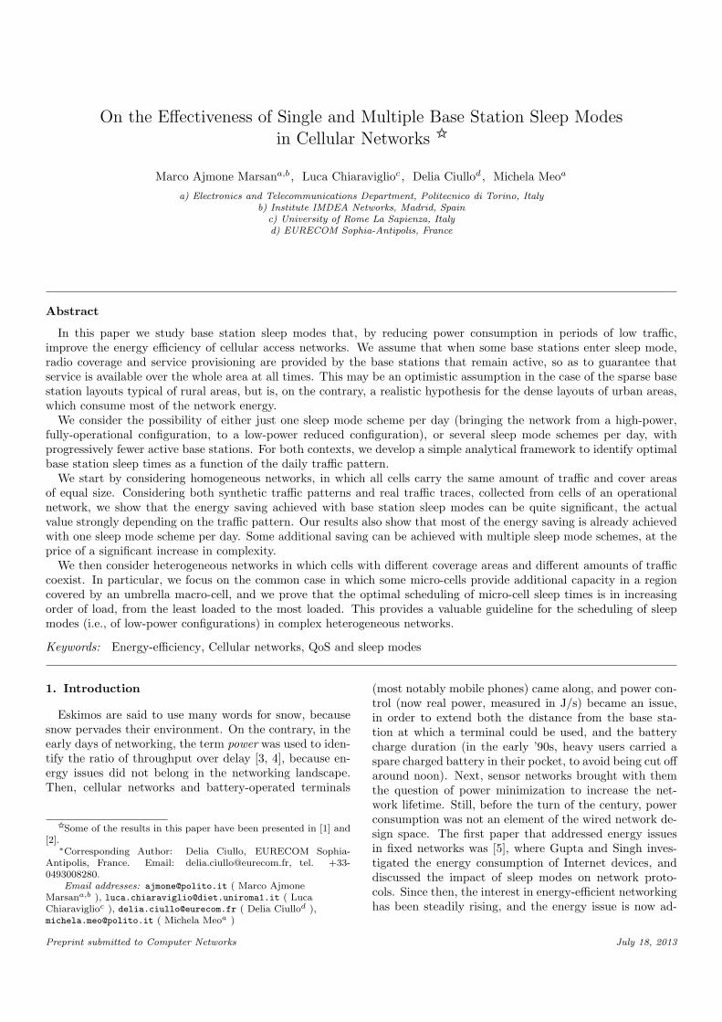
Figure 7: Hexagonal three-sectorial configuration: 3 cells being putto sleep out of 4 (top) and 8 out of 9 (bottom).

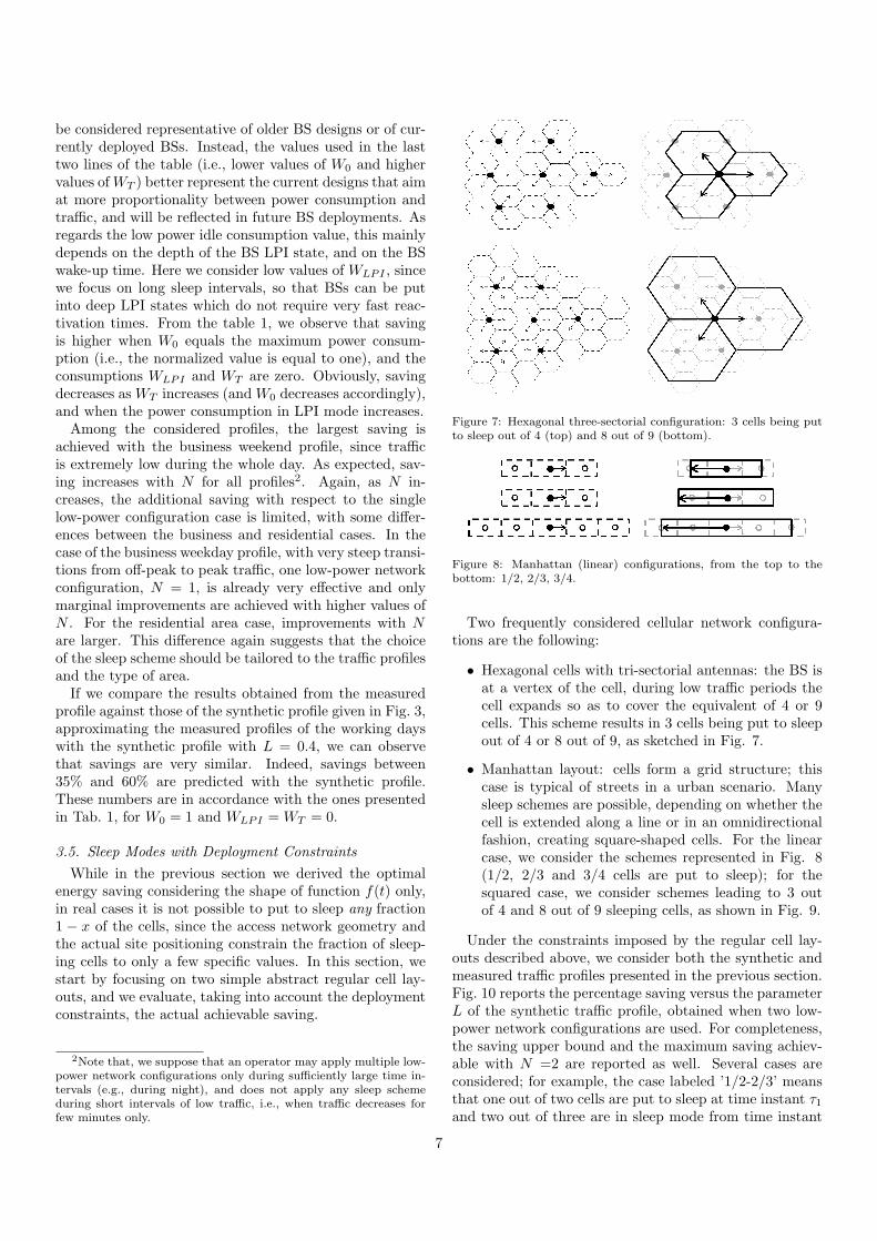
Figure 8: Manhattan (linear) configurations, from the top to thebottom: 1/2, 2/3, 3/4.

Two frequently considered cellular network configura-tions are the following:

• Hexagonal cells with tri-sectorial antennas: the BS isat a vertex of the cell, during low traffic periods thecell expands so as to cover the equivalent of 4 or 9cells. This scheme results in 3 cells being put to sleepout of 4 or 8 out of 9, as sketched in Fig. 7.

• Manhattan layout: cells form a grid structure; thiscase is typical of streets in a urban scenario. Manysleep schemes are possible, depending on whether thecell is extended along a line or in an omnidirectionalfashion, creating square-shaped cells. For the linearcase, we consider the schemes represented in Fig. 8(1/2, 2/3 and 3/4 cells are put to sleep); for thesquared case, we consider schemes leading to 3 outof 4 and 8 out of 9 sleeping cells, as shown in Fig. 9.

Under the constraints imposed by the regular cell lay-outs described above, we consider both the synthetic andmeasured traffic profiles presented in the previous section.Fig. 10 reports the percentage saving versus the parameterL of the synthetic traffic profile, obtained when two low-power network configurations are used. For completeness,the saving upper bound and the maximum saving achiev-able with N =2 are reported as well. Several cases areconsidered; for example, the case labeled ’1/2-2/3’ meansthat one out of two cells are put to sleep at time instant τ1and two out of three are in sleep mode from time instant

7

Table 1: Measured traffic patterns: maximum achievable saving for various number of network configurations

Power Consumption Model Network configuration S[%] S[%] S[%] S[%]Business WE Business WD Residential WE Residential WD

WLPI=0.0 W0=1.0 WT=0.0

Upper Bound 91.40 61.86 50.10 59.90N = 3 89.85 50.96 40.06 49.21N = 2 89.28 46.57 34.55 44.91N = 1 84.30 42.01 26.61 33.90

WLPI=0.1 W0=0.8 WT=0.1

Upper Bound 80.46 52.68 42.16 50.90N = 3 79.10 43.39 33.71 41.82N = 2 78.62 39.65 29.07 38.16N = 1 74.21 35.77 22.40 28.81

WLPI=0.0 W0=0.6 WT=0.4

Upper Bound 86.38 48.99 37.45 46.97N = 3 84.92 40.35 29.94 38.58N = 2 84.38 36.88 25.82 35.21N = 1 79.67 33.27 19.90 26.58

WLPI=0.1 W0=0.4 WT=0.5

Upper Bound 67.26 35.50 26.60 33.91N = 3 66.12 29.24 21.27 27.86N = 2 65.70 26.72 18.34 25.42N = 1 62.04 24.10 14.13 19.19

Figure 9: Manhattan (squared) configurations: 3/4 (top) and 8/9(bottom).

τ2. For small values of L (right part of the curves) thelargest saving is obtained by putting into sleep mode thelargest fraction of cells (configuration 8/9). These valuesof L correspond to cases in which the transient from thepeak to the off-peak traffic is short (steep decrease) andit is convenient to put to sleep a larger number of cellsfor a (slightly) shorter time. However, the saving rapidlydecreases as L increases, and the schemes that correspondto put to sleep a smaller number of cells, such as 1/2 or2/3, become more convenient. Note that for low valuesof L (that correspond to low overall daily traffic loads),the results for regular topologies are quite similar to thosewith no topological constraints. The effect of topology be-comes relevant at high load, in cases in which only a smallfraction of cells can be switched off, but this may not bepossible due to the topological structure.

Consider now the measured traffic profiles of the busi-ness area. Fig. 11 reports the network saving that canbe achieved with two low-power network configurations,considering the weekday traffic pattern. The graph, withits level curves, shows the saving achievable when the first

00.20.40.60.810

10

20

30

40

50

60

70

80

90

100

Parameter L

Sav

ing

[%]

Upper BoundDouble Configuration (Max)1/2−2/31/2−3/42/3−3/43/4−8/9

Figure 10: Two low traffic network configurations: network savingversus the parameter L for the synthetic traffic profile.

configuration is entered at τ1 and the second one at τ2.Observe that, by the definition of τi, the white area forwhich τ1 > τ2 corresponds to non admissible points. Themarkers localize the cases possible with regular topologies.Saving is maximized when the first configuration occurs inthe evening, and the second is during night. The strangebehavior of the curves corresponding to the vertical slicearound lunch time is due to the corresponding gap in thetraffic profile, see Fig. 5. Interestingly, regular topologies,identified by the markers in the figure, achieve good sav-ing, pretty close to the maximum possible. This suggeststhat, even in presence of some topological and physicallayout constraints, sleep schemes can be quite effective,and shows that a simple analytical model, coupled with asynthetic traffic pattern, leads to potential energy savingsestimates that are similar to what is achievable throughmore detailed models.

8

11:00 15:00 19:00 23:00 03:0011:00

15:00

19:00

23:00

03:00

τ1

τ 2

0

5

10

15

20

25

30

35

40

1/2−2/31/2−3/42/3−3/43/4−8/9

Figure 11: Business cell - weekday profile: network saving with twolow traffic network configurations.

4. Heterogeneous Networks

In the previous section, we have considered homoge-neous networks in which all BSs are characterized by thesame power consumption and the same traffic load, andcells are equivalent and interchangeable in terms of cov-erage, so that any number of cells can be put into sleepmode while the remaining active cells guarantee coverage.We now consider the case of heterogeneous networks, i.e.,networks in which cells of different size and load coex-ist (possibly covered by BSs of different technologies). Inparticular, we consider a scenario in which an umbrella(macro) cell provides coverage over an area, and K micro-cells are deployed to provide additional capacity. To saveenergy, micro-cells can be put to sleep when their trafficis low and can be carried by the macro-cell; in this case,their traffic cannot be carried by the other micro-cells dueto coverage limits.As before, we assume that the traffic profile f(t) of the

umbrella cell is decreasing with t and is symmetric aroundT/2. The micro-cells have the same traffic profile shapeas the macro-cell, since this is given by the typical humanbehavior that is assumed to be uniform in a given area;however, based on the cell size and user density, the shapecan be scaled of a given factor, i.e., micro-cell i supportsa traffic that is αif(t). We assume that micro-cell i con-sumes an amount of power equal to

P (i)(t) = W(i)LPI +W

(i)0 +W

(i)T αif(t) (18)

while the macro-cell consumes

P (M)(t) = W(M)LPI +W

(M)0 +W

(M)T f(t) (19)

In the case of homogeneous networks, a low-power net-work configuration Φ was defined by the fraction of activecells x and the corresponding smallest instant τ in whichthe load constraint (2) was satisfied. Here, in the hetero-geneous case, we define a low-power configuration by spec-ifying the active/sleep state, micro-cell by micro-cell. Inparticular, a configuration Ψ can be represented through

an indicating function, I(Ψ)(k) with k = 1, · · · ,K, thatdefines the state of the micro-cell k, that can be eithersleeping or active,

I(Ψ)(k) =

{

1 if micro-cell k is sleeping0 if micro-cell k is active

(20)

The configuration Ψ is feasible at time t if the followingload constraint condition holds,

(

1 +

K∑

k=1

αkI(Ψ)(k)

)

f(t) < 1 (21)

This condition imposes that the load in the macro-cell doesnot exceed the maximum allowable load, namely 1; andthat the macro-cell is receiving the traffic of all the micro-cells that are in sleep mode, i.e., for which I(Ψ)(k) = 1.Assuming, as before, that f(t) is symmetric and decreasingin [0, T/2], the scheme Ψ becomes feasible at time τ , with,

τ = f−1

(

1

1 +∑K

k=1 αkI(Ψ)(k)

)

(22)

Putting to sleep micro-cell k at time t is convenient interms of energy consumption when the additional costthat the macro-cell has to sustain to carry the traffic ofmicro-cell k is smaller than the saving achieved by puttingmicro-cell k into sleep mode; i.e., when the following savingconstraint holds,

W(k)0 +W

(k)T αkf(t) ≥ W

(M)T αkf(t) (23)

We define, then, a scheme Ψ to be convenient at time t if(23) holds for every micro-cell k in sleep mode. When Ψis applied, the power saving is equal to,

S(Ψ)(t) =

K∑

k=1

[

W(k)0 + (W

(k)T −W

(M)T )αkf(t)

]

I(Ψ)(k)

(24)To find the optimal multiple low-power configuration

sleep scheme, we first define the set of all possible configu-rations, C. The set C contains 2K elements that correspondto all possible combinations of any micro-cell being eitheractive or sleeping, C = {Ψi} with i = 0, · · · , 2K . At timet, the set of the feasible and convenient configurations isdefined by those configurations Ψi that, at t, satisfy boththe load constraint (21) and the saving constraints (23),

C(t) ⊂ C, with

C(t) ={

Ψi

∣

∣

∣

(

1 +∑K

k=1 αkI(Ψi)(k)

)

f(t) < 1}

∩{

Ψi

∣

∣

∣∀k, I(Ψi)(k)

[

W(k)0 + (W

(k)T −W

(M)T )αkf(t)

]

≥ 0}

Among the configurations in C(t), an optimal choice,Ψ∗(t) ∈ S(t), is given by one of the configurations thatmaximizes the saving in (24),

Ψ∗(t) = maxΨi∈C(t)

S(Ψ)(t) (25)

9

We focus now on the (realistic) case in which the cost

to carry a unit of traffic in the macro-cell, W(M)T is larger

than the costs to carry the same amount of traffic in the

micro-cells, W(k)T . Indeed, the larger transmission power

makes this happens most of the time [24].

This assumption means that in (24) the terms W(k)T −

W(M)T are negative, and the larger the traffic αkf(t) is, the

smaller the saving is.Lemma 1: Under the two following conditions,

1. all micro-cells have the same power consumption

model, i.e., W(k)LPI = WLPI , W

(k)0 = W0 and W

(k)T =

WT ;

2. the cost to carry a unit of traffic through themacro-cell is higher than through the micro-cell, i.e.,

W(M)T > WT ;

the “least-loaded” policy, consisting in putting the micro-cells into sleep mode in reverse order w.r.t. their load, i.e.,from the least loaded to the most loaded, is optimal interms of the achieved saving.

Proof. Consider a configuration Ψi. The termf(t)

∑Kk=1 αkI

(Ψi)(k) represents the traffic increment thatthe macro-cell undergoes when Ψi is applied; where αkf(t)is the contribution to traffic due to micro-cell k going tosleep mode. Now, since f(t) is monotonically decreasing in[0, T/2], the time τi at which Ψi can be applied dependson this traffic increment; considering two configurationsΨi and Ψj ,

τi < τj if

K∑

k=1

αkI(Ψi)(k) <

K∑

k=1

αkI(Ψj)(k) (26)

That is, the time order in which the configurations becomefeasible (i.e., satisfy the load constraint) is according toincreasing values of the total traffic added to the macro-cell.Denote by φi the time at which putting to sleep micro-

cell i becomes convenient; from (23),

φi = f−1

W0

αi

(

W(M)T −WT

)

(27)

Since f(t) is monotonically decreasing, the times φi areordered according to increasing values of the individual

micro-cell load, αi, that is:

φi < φj if αi < αj (28)

Now, consider the set AV ⊂ C of all the configurationsΨi corresponding to V micro-cells in sleep mode,

AV =

{

Ψi

∣

∣

∣

K∑

k=1

I(Ψi)(k) = V

}

Among these, the scheme ΨV that saves the most, corre-sponds to putting to sleep the V least loaded cells. Indeed,from (24), the saving is

S(ΨV ) = VW0 +

K∑

k=1

(

WT −W(M)T

)

αkf(t)I(ΨV )(k) (29)

and, since the second term is negative, due toW(M)T > WT ,

the saving is maximized if the amount of traffic of thesleeping cells is smallest.Moreover, among the schemes in AV , ΨV is also the one

that becomes feasible at the earliest time, since accordingto (27), the micro-cells can be put to sleep in the order ofthe amount of carried load.When ΨV satisfies the constraint (23), its saving is

larger than the best scheme of AV−1, that is ΨV−1: i.e.,S(ΨV ) > S(ΨV −1) because the contribution to saving givenby each micro-cell k that is sleeping is positive:

W0 +(

WT −W(M)T

)

αkf(t) > 0 (30)

and the saving S(ΨV ) is composed of the sum of the samesavings of ΨV−1 plus a positive term, corresponding to theadditional cell that is sleeping in ΨV w.r.t. ΨV−1.

Denote by tV the time instant in which ΨV becomesfeasible and convenient. By definition of tV , in the intervalbetween tV and tV+1, no configuration can save more thanΨV , so that in the interval [tV , tV+1] the configuration ΨV

is optimum, in the sense that it achieves the maximumpossible saving.By extending this reasoning to the other time intervals,

we conclude that putting to sleep micro BS from the leastloaded to the most loaded, leads to the maximum saving.

4.1. Case Study

In the following, we finally show how the previous resultscan be applied to a realistic cell deployment.We consider a portion of the central area of the city

of Munich, in Germany, which corresponds to a square of800 x 800 m, comprising 1 macro-cell, 8 micro-cells, and10 femto-cells. Femto-cells are deployed to provide addi-tional capacity during peak hours in indoor environments.However, we do not consider them in the sleep schemes,since they consume a negligible amount of power, and theircoverage is extremely limited, so that the probability thatusers can access them in periods of low load is very small.The micro-cells are served by isotropic antennas, each withtransmission power of 1 W, while the macro-cell has atri-sectorial antenna with 40 W emitted power. We as-sume that the total power consumption of the macro-cellis seven times higher than the one of a micro-cell [25]. Fig.12 presents a map of the considered area, together with aside view (at the bottom of the figure).The area coverage is computed from the signal strength

received on the users’ pilot channel. To estimate the chan-nel conditions, i.e., the path losses, we use the results of

10

Figure 12: Case study: Map with cell identifiers (SC = micro cell).Aerial view (top) and side view (bottom).

a tool developed by Alcatel-Lucent, called Wireless Sys-tem Engineering (WiSE) [26], that is based on ray-tracingtechniques. We refer the reader to [27] for further detailson users’ coverage computation.

The network is planned assuming that in the coverageareas of the micro-cells, the users density is 5 times higherthan in the remaining area. As traffic profile, we considerthe weekday profiles of either the business or the residen-tial areas, see Figs. 5 and 6. Moreover, we assume that atthe peak traffic hour, the most loaded cell carries a nor-malized traffic load equal to 1. During low traffic periods,micro-cells enter sleep mode, and the macro-cell acts as anumbrella cell which is never switched off. We assume thatthe macro-cell can guarantee full coverage, even when allthe other cells are put into sleep mode.

Table 2 summarizes the network saving obtained underdifferent schemes, for both the considered profiles, and fordifferent power consumption models. As already noted inSection 3, the highest saving is achieved when the powerconsumption W0 is maximum and the power consumed inLPI state is zero, with saving that slightly decreases asWT increases. Moreover, the increase of WLPI makes thesleep mode scheme less convenient.

Saving of the order of 15-25% can be achieved with onelow-power network configuration. The saving increases sig-nificantly with two low-power configurations (up to 32%),while the saving increment is marginal as the number ofconfigurations further increases. Note that, in the case of

one low-power configuration, the savings achievable withthe business traffic profile are higher, due to the highersteepness of the transients; the maximum savings are, in-stead, comparable for the two traffic profiles.Finally, Figs. 13 and 14 show the number of active micro

BSs versus time, considering the weekday traffic profiles:the cases of one, two, three low-power configurations, arereported. For completeness, the curve obtained with theLeast-Loaded policy is also shown (label ’Maximum’): thisrepresents a lower bound on the minimum number of activeBSs, and corresponds to the maximum achievable saving.

5. Implementation Issues

In this section we briefly discuss some implementationissues related to the introduction of sleep modes in BSs.The first fundamental implementation issue concerns

the algorithm to decide the sleep mode patterns and con-figurations. In particular, the algorithm might be offlineor online. In the offline case, the decision is taken based onhistorical data about the traffic amount and pattern; his-torical data, possibly combined with forecast about trafficvariations, are used to decide when and which BSs shouldgo to sleep in a given area. The decision is thus static anddoes not adapt to the actual network conditions. This issimilar to what is usually done by operators when they areplanning their networks. Online algorithms, on the con-trary, decide the BS mode based on online measurements.Through these algorithms, the network adapts to actualtraffic conditions. Centralized or distributed algorithmscan be implemented: the first typically involve more in-formation exchange between BSs and network controllerentities, but is more efficient in terms of finding the opti-mal sleep configuration; the latter requires less signaling,but typically finds sub-optimal schemes.Some critical issues are also related to the BS wake

up times. The amount of time required for a BS acti-vation/deactivation depends on the sleep state level of theBS: the deeper the sleep level is, the higher the power sav-ing is, but the longer the transition time between sleep andactive states is. A careful trade-off should then be decidedbetween the depth of the sleep mode, and consequentlythe saving, and the need for short state transition times.Furthermore, in the case of online algorithms, fast trafficvariations may lead to ping-pong effects, i.e., frequent al-ternations of switch on and off of the same devices. Tosolve these problems, authors in [28] proposed to intro-duce a guard interval to anticipate bursts of arrivals byswitching on additional BSs, and a hysteresys time beforeputting BSs to sleep.In addition, the possibility of faults due to frequent

switch-on and switch-off transients must be considered.The hardware of present generations of BSs is not designedfor these usage patterns. New generation of equipmentmust allow this possibility.The fact that we proved in this paper that very few

switch on/off per day (typically one) are sufficient to ob-

11

Table 2: Case Study: savings with different network configurations

Power Consumption Model Network configuration S[%] S[%]Business weekday Residential weekday

WLPI=0.0 W0=1.0 WT=0.0

Single (7/9) 26.39 19.73Double (4/9)-(7/9) 31.96 32.16Triple (2/9)-(4/9)-(7/9) 34.64 33.43Maximum (Least-Loaded) 38.27 38.79

WLPI=0.1 W0=0.8 WT=0.1

Single (7/9) 23.18 17.24Double (4/9)-(7/9) 27.84 27.73Triple (2/9)-(4/9)-(7/9) 30.06 28.78Maximum (Least-Loaded) 33.16 33.30

WLPI=0.0 W0=0.6 WT=0.4

Single (7/9) 24.69 17.92Double (4/9)-(7/9) 28.73 27.31Triple (2/9)-(4/9)-(7/9) 30.05 28.18Maximum (Least-Loaded) 33.55 32.21

WLPI=0.1 W0=0.4 WT=0.5

Single (7/9) 18.99 13.53Double (4/9)-(7/9) 21.71 20.00Triple (2/9)-(4/9)-(7/9) 22.94 20.59Maximum (Least-Loaded) 25.10 23.27

tain most of the energy gain is quite relevant both for thereduction of the impact of activation/deactivation tran-sient times, and for the reduction of faults.For an effective implementation of sleep modes, a net-

work operator should first weight the potential benefits,which we have characterized in this paper, and then care-fully consider the most convenient sleep mode level, hys-teresis and guard interval values, scheduling BS activa-tions and deactivations based on the network traffic statis-tics/forecasts. Our simple models indicate that the poten-tial energy savings are so large, that significant benefitsexist in practice, in spite of the possible reductions due toimplementation issues.

6. Conclusions

In this paper we investigated the energy saving that canbe achieved in cellular access networks by optimizing theuse of sleep modes according to daily traffic variations.By assuming that, as is usually the case in dense ur-

ban environments, when a cell is in sleep mode, coveragecan be filled by its neighbors, we derived expressions forthe optimal energy saving when the network can moveamong N different low-power network configurations, andan expression for a theoretical upper bound of saving. Ourderivation proves that energy savings, as well as the opti-mal choice of the periods in which different low-power con-figurations should be adopted, are functions of the dailytraffic patterns. Thus, the first main insight deriving fromthis work is that the daily traffic pattern plays a centralrole in the design of dynamic network planning schemesthat adopt sleep modes.The numerical results we presented, derived for many

cell layouts, traffic patterns, and power consumption mod-els, provide several additional interesting insights. First

of all, for the considered real traffic patterns, savings arequite significant: they reach 90% in the case of weekendtraffic in business areas, and are of the order of 30-40%in other cases. This is an important signal indicating thatsleep modes can indeed be a useful tool for energy-efficientnetworking. Second, we have shown that significant sav-ings can be achieved with only one low-power networkconfiguration per day, while the benefit of multiple con-figurations is minor. This is especially true in the case inwhich the traffic profile has a steep transition from the off-peak hours to on-peak hours, like in business areas duringweekdays. This is also an important message, because itshows that most of the gains can be obtained with limitedeffort on the side of network management. Third, savingscan be strongly influenced by the different power consum-ption components of a BS. Indeed, sleep modes are moreeffective when the power necessary to carry zero traffic ishigh, and both the power consumption in LPI mode andthe power proportional to the traffic are low.Finally, we have also proved that in presence of deploy-

ment of BSs for additional capacity provisioning, the op-timal order in which the BSs should enter sleep mode, i.e.the order that jointly maximizes energy saving and mini-mizes the number of BS transients, consists in putting cellsto sleep according to increasing values of their load. Thistoo, is a relevant result for network management.Our results provide a tangible incentive for cellular net-

work operators to implement sleep modes in their net-works.

Acknowledgement

The authors wish to thank Alberto Conte and Afef Fekiof Alcatel-Lucent Bells Labs for providing data about thereal BS deployment and coverage in downtown Munich.

12

11:00 15:00 19:00 23:00 03:00 07:00 11:000

1

2

3

4

5

6

7

8

Time

Num

ber

of M

icro

Bas

e S

tatio

ns O

n

Maximum

(a) Maximum

11:00 15:00 19:00 23:00 03:00 07:00 11:000

1

2

3

4

5

6

7

8

Time

Num

ber

of M

icro

Bas

e S

tatio

ns O

n

Single Configuration

(b) Single

11:00 15:00 19:00 23:00 03:00 07:00 11:000

1

2

3

4

5

6

7

8

Time

Num

ber

of M

icro

Bas

e S

tatio

ns O

n

Double Configuration

(c) Double

11:00 15:00 19:00 23:00 03:00 07:00 11:000

1

2

3

4

5

6

7

8

Time

Num

ber

of M

icro

Bas

e S

tatio

ns O

n

Triple Configuration

(d) Triple

Figure 13: Business weekday: number of active micro BSs versus time for different network configurations.

The research leading to these results has received fundingfrom the European Union Seventh Framework Programme(FP7/2007-2013) under grant agreement n. 257740 (Net-work of Excellence TREND).

[1] M. Ajmone Marsan, L. Chiaraviglio, D. Ciullo, M. Meo, OptimalEnergy Savings in Cellular Access Networks, GreenComm’09 -1st International Workshop on Green Communications, Dresden,Germany, June 2009.

[2] M. Ajmone Marsan, L. Chiaraviglio, D. Ciullo, M. Meo, Multi-ple Daily Base Station Switch-Offs in Cellular Networks, FourthInternational Conference on Communications and Electronics(ICCE’12), Hue, Vietnam, August 2012.

[3] A. Giessler, J. Haenle, A. Koenig, E. Pade, Free buffer allocation:An investigation by simulation, Computer Networks, Vol.2, n.3,July 1978, pp. 191-208.

[4] L. Kleinrock, Power and Deterministic Rules of Thumb forProbabilistic Problems in Computer Communications, ICC 79,Boston, MA, USA, June 1979.

[5] M. Gupta, S. Singh, Greening of the Internet, ACM SIGCOMM2003, Karlsruhe, Germany, August 2003.

[6] TREND Project, http://www.fp7-trend.eu.[7] K. Son, B. Krishnamachari, SpeedBalance: Speed-Scaling-Aware

Optimal Load Balancing for Green Cellular Networks, IEEE IN-FOCOM Mini-conference 2012, Orlando, FL, USA, March, 2012.

[8] O. Arnold, F. Richter, G. Fettweis, and O. Blume, Power con-sumption modeling of different base station types in heteroge-neous cellular networks, in Proc. of 19th Future Network andMobileSummit, 2010.

[9] J. Lorincz, T. Garma, G. Petrovic, Measurements and Modellingof Base Station Power Consumption under Real Traffic Loads,

Sensors, Vol. 12, pp. 4281-4310.[10] J.T. Louhi, Energy efficiency of modern cellular base stations,

INTELEC 2007, Rome, Italy, September-October 2007.[11] H. O. Scheck, J. Louhi, Energy Efficiency of Cellular Networks,

W-GREEN 2008, Lapland, Finland, September 2008.[12] Global Action Plan, An inefficient truth,

http://www.globalactionplan.org.uk/, Global Action PlanRep., 2007.

[13] M. Hodes, Energy and power conversion: Atelecommunication hardware vendor’s perspective,http://www.peig.ie/pdfs/ALCATE~1.PPT, Power ElectronicsIndustry Group, 2007.

[14] Bi-annual Report November 2010, Green Power for Mo-bile, GSMA. Available: http://www.gsmworld.com/our-work/mobileplanet/green power for mobile/renewable energy networks.htm.

[15] H. Claussen, L. T. W Ho, and F. Pivit, Effects of joint macrocelland residential picocell deployment on the network energy effi-ciency, IEEE 19th International Symposium on Personal, Indoorand Mobile Radio Communications (PIMRC), 2008, Cannes,France, September 2008.

[16] Z. Niu, Y. Wu, J. Gong, Z. Yang, Cell zooming for cost-efficientgreen cellular networks, IEEE Communication Magazine, Vol.48, n. 11, pp. 74-79, November 2010.

[17] L. Chiaraviglio, D. Ciullo, M. Meo, M. Ajmone Marsan, Energy-Aware UMTS Access Networks, W-GREEN 2008, Lapland, Fin-land, September 2008.

[18] M. Ajmone Marsan, L. Chiaraviglio, D. Ciullo, M. Meo, Energy-Efficient Management of UMTS Access Networks, ITC 21 -21st International Teletraffic Congress, Paris, France, Septem-ber 2009.

[19] E. Oh, B. Krishnamachari, X. Liu, Z. Niu, Toward dynamic en-

13

22:30 02:30 06:30 10:30 14:30 18:30 22:300

1

2

3

4

5

6

7

8

Time

Num

ber

of M

icro

Bas

e S

tatio

ns O

n

Maximum

(a) Maximum

22:30 02:30 06:30 10:30 14:30 18:30 22:300

1

2

3

4

5

6

7

8

Time

Num

ber

of M

icro

Bas

e S

tatio

ns O

n

Single Configuration

(b) Single

22:30 02:30 06:30 10:30 14:30 18:30 22:300

1

2

3

4

5

6

7

8

Time

Num

ber

of M

icro

Bas

e S

tatio

ns O

n

Double Configuration

(c) Double

22:30 02:30 06:30 10:30 14:30 18:30 22:300

1

2

3

4

5

6

7

8

Time

Num

ber

of M

icro

Bas

e S

tatio

ns O

n

Triple Configuration

(d) Triple

Figure 14: Residential weekday: number of active micro BSs versus time for different network configurations.

ergy efficient operation of cellular network infrastructure, IEEECommunication magazine, Vol. 49, n. 6, pp. 56-61, June 2011.

[20] K. Son, H. Kim, Y. Yi and B. Krishnamachari, Base Sta-tion Operation and User Association Mechanisms for Energy-Delay Tradeoffs in Green Cellular Networks, IEEE Journal onSelected Area in Communications: Special Issue on Energy-Efficient Wireless Communications, Vol. 29, No. 8, pp. 1525 -1536, September 2011.

[21] C. Peng, S. B. Lee, S. Lu, H. Luo, H. Li, Traffic-Driven PowerSaving in Operational 3G Cellular Networks, ACM MobiCom2011, Las Vegas, Nevada, USA, September 2011.

[22] L.i Saker, S. E. Elayoubi, Sleep mode implementation issues ingreen base stations, PIMRC 2010, Istanbul, Turkey, September2010.

[23] M. Ajmone Marsan, M. Meo, Energy Efficient Wireless InternetAccess with Cooperative Cellular Networks, Computer Networks,2011, Vol. 55,, No. 2, pp. 386 - 398.

[24] G. Auer et al., How much Energy is needed to run a WirelessNetwork?, IEEE Wireless Commun. Mag., vol. 18, no. 5, pp.4049, October 2011.

[25] G. Auer, V. Giannini, I. Godor, P. Skillermark, M. Olsson, M.A. Imran, D. Sabella, M. J. Gonzalez., C. Desset, O. Blume, Cel-lular Energy Efficiency Evaluation Framework, GreeNet work-shop, in proc. of VTC Spring 2011.

[26] S. Fortune et al., WiSE Design of Indoor Wireless Systems:Practical Computation and Optimization, IEEE ComputationalScience & Engineering, vol. 2, no. 1, pp. 58-68, spring 1995.

[27] M. Ajmone Marsan, L. Chiaraviglio, D. Ciullo, M. Meo, Switch-Off Transients in Cellular Access Networks with Sleep Modes,GreenComm 4, Kyoto, Japan, June 2011.

[28] L. Saker, S. E. Elayoubi, Sleep mode implementation issues ingreen base stations, IEEE PIMRC, Istanbul, Turkey, September

2010.

14