on the dynamics of debris flows
TRANSCRIPT

Master Thesis in Geosciences
On the dynamics of debris flows Case study Fjærland, Western Norway - a debris flow triggered by a natural dam breach
Hedda Breien
On the dynamics of debris flows Case study Fjærland, Western Norway – a debris flow
triggered by a natural dam breach
Hedda Breien
Master Thesis in Geosciences
Discipline: Environmental Geology and Geohazards
Department of Geosciences
Faculty of Mathematics and Natural Sciences
UNIVERSITY OF OSLO June 2005

III
© Hedda Breien, 2005
Advisers: Dr. Anders Elverhøi (UiO) and Dr. Kaare Høeg (UiO)
This work is published digitally through DUO – Digitale Utgivelser ved UiO
http://www.duo.uio.no
It is also catalogued in BIBSYS (http://www.bibsys.no/english)
All rights reserved. No part of this publication may be reproduced or transmitted, in any form or by any means, without permission.
Cover photo: C. Harbitz.

IV
Acknowledgements
First of all, I would like to take the opportunity to thank my two supervisors Professor
Anders Elverhøi and Professor Kaare Høeg. Anders; you have provided irreplaceable help
and inspiration, as well as valuable contact with local residents in Fjærland. And not to
forget: your sincere involvement and participation! Special thanks to Kaare for all your
advices and your encouraging words. If it was not for you and your fantastic lessons in
engineering geology and geomechanics, I would never have found such an interesting field
of study. I am lucky to know such a wise and nice person.
This thesis has been part of the Slide dynamics and mechanics of disintegration project at the
International Centre for Geohazards (ICG). Many thanks go to all ICG and NGI for letting
me stay in such a nice and encouraging research environment and for the help and laughter
you all have provided. Special thanks to Dr. Fabio De Blasio at ICG for struggling with the
BING-code. You are my guide and hero in rheology and modelling! Beyond that; I would
never have got a nicer office-mate. I hope our cooperation will continue.
From the University of Oslo I am particularly grateful to Trond Eiken. The terrain modelling
part of my thesis would never have been completed without you! Thank you for your
patience and all your help during frustrating hours.
Thanks to all inhabitants of Supphelledalen for your hospitality and the valuable information
you all have provided.
I would also like to honour my family for patience and supporting words throughout years of
studies. I hope to get more time for visits in the future!
Finally, I wish to thank my boyfriend Geir Ole for unconditional love and support.
Hedda Breien
Oslo, June 2005.

V
Abstract
Debris flows represent a major threat to human life and property. Due to their ability of
entraining material and reaching long run-outs, they have a potential of causing massive
damage.
There are many studies on debris flow dynamics. Still, the topic reveals a number of
challenges in understanding the forces involved and in representing them numerically. In
this respect the recent debris flow in Fjærland, Western Norway, is looked upon as a unique
full scale experiment with its 1000 m height drop and 3000 m long run-out.
The Fjærland case includes the breach of a moraine ridge damming a glacial lake, the
additional water coming from the glacier, and its resulting flood. The study of this case
illustrates how a water flood can evolve into a full debris flow through bulking. Even though
the event started out as a flood of water, the study has revealed that the deposited materials
and the degree of erosion also result from a significant grain-to-grain contact. It is seen that
treating such events as floods is not appropriate where the height drop is large and the bed
material erodible.
The primary objective of the thesis has been to provide a thorough documentation and
description of the event. Through this work, several eyewitnesses have been interviewed,
and detailed pre- and post flow terrain models have been developed through laser scanning
and photogrammetry in the purpose of estimating the volume involved in the debris flow.
The same terrain data have been employed in a numerical model (BING), trying to simulate
the dynamics of the flow. The model uses a Bingham rheology, but is modified to include
Coulomb friction and entrainment by Dr. Fabio De Blasio of ICG. The expanded BING-
model predicts a run-out, erosion depth and a volume encouragingly similar to what is seen
in nature. However, many physical simplifications have had to be introduced, and challenges
for further studies are several.
The study reveals the necessity for a dynamical model which, depending on the contents and
properties of the material involved, includes both viscous, plastic and frictional forces,
allows forces and properties to vary in time and space, as well as taking material entrainment
into account.

VI
A most interesting topic for further study is the factor of entrainment. Until now, this
phenomenon is not fully understood. The thesis tries to illustrate the phenomenon with the
recently accumulated data. One of the findings of the thesis is the recognition of a feedback
mechanism, where volume growth increases the entrainment of bed material, which again
increases the volume of the flow. For erosion, the volume of the mass flow seems more
important than slope angle, at least in slopes steeper than a certain value. This was also
recognised in the numerical modelling, shown by an exponential increase in volume. The
ability of volume growth can be the explanation for debris flows with very far-reaching run-
outs.
There is historical evidence that similar debris flow events have happened in Fjærland twice
during the last century. An event like the one that occurred 8 May 2004 is also likely to
happen again - in Fjærland as well as any other place where large volumes of water are
released at high altitude. This study is therefore important also in the evaluation of hazards
related to other glaciers, lakes and dams as well as to landslide-triggered debris flows.

VII
Table of Contents
1. Introduction ................................................................................................ 1
1.1 Purpose and scope ................................................................................................................. 2
1.2 Setting..................................................................................................................................... 3
1.3 Collection of data................................................................................................................... 4
2. Observations ............................................................................................... 6
2.1 Eyewitness observations ....................................................................................................... 6 2.1.1 A) From the cabin Flatbrehytta, 994 m.a.s.l. .............................................................................. 8 2.1.2 B) From Øygardsneset, 25 m.a.s.l............................................................................................... 9 2.1.3 C) From Supphella 30 m.a.s.l. .................................................................................................. 12 2.1.4 D) From Mundal ....................................................................................................................... 12
2.2 Field observations................................................................................................................ 12 2.2.1 The moraine ridge breach ......................................................................................................... 13 2.2.2 Debris flow path........................................................................................................................ 15 2.2.3 Soil material .............................................................................................................................. 19 2.2.4 Deposits along the track............................................................................................................ 20 2.2.5 Depositional fan ........................................................................................................................ 23 2.2.6 Mud deposit .............................................................................................................................. 25
2.3 Description of the Fjærland torrent event using eyewitness statements and field
observations................................................................................................................................... 26
2.4 The deposit – Brazil nut effect and bridging .................................................................... 28
2.5 Total duration...................................................................................................................... 29
3. Previous debris flow events in Fjærland................................................ 31
3.1 Future events ....................................................................................................................... 34
4. Terrain modelling..................................................................................... 35
4.1 Aerial photos and photogrammetry .................................................................................. 35 4.1.1 Stereo model ............................................................................................................................. 35
Problems.............................................................................................................................................. 36

VIII
4.1.2 Orthophotos............................................................................................................................... 36 4.1.3 Digital terrain models................................................................................................................ 36 4.1.4 Resolution ................................................................................................................................. 38
4.2 LIDAR laser scanning......................................................................................................... 40 4.2.1 Errors......................................................................................................................................... 41
4.3 Laser vs. aerial photos ........................................................................................................ 44 4.3.1 Volume estimate........................................................................................................................ 44 4.3.2 Visualisation using profiles and 3D models.............................................................................. 44
5. Glaciology and the Supphellebreen glacier ........................................... 45
5.1 Glaciers in Norway.............................................................................................................. 45
5.2 The glacier Supphellebreen ................................................................................................ 46 5.2.1 Characteristics ........................................................................................................................... 46 5.2.2 History....................................................................................................................................... 48
5.3 Glacier hydrology................................................................................................................ 48 5.3.1 Formation of a channel.............................................................................................................. 48 5.3.2 Discharge variations.................................................................................................................. 50 5.3.3 Storage of water ........................................................................................................................ 51
5.4 Glacial lakes and Jøkulhlaups............................................................................................ 52
5.5 History of Supphellebreen lake drainage.......................................................................... 53
6. Estimated water volume involved in the flow ....................................... 55
6.1 Glacial lake area.................................................................................................................. 55
6.2 Additional water from the glacier...................................................................................... 58 6.2.1 Temperature and melting .......................................................................................................... 59
6.3 Estimated water volume considering cross sections......................................................... 61 6.3.1 Scenarios ................................................................................................................................... 63
7. The moraine ridge breach....................................................................... 66
7.1 Ridge failure ........................................................................................................................ 66 7.1.1 Failure mechanisms................................................................................................................... 67 7.1.2 The breaching process............................................................................................................... 68
7.2 Possible ice core in Fjærland.............................................................................................. 71
8. Estimated sediment volume involved in the flow.................................. 73

IX
8.1 Characteristics of the till..................................................................................................... 73
8.2 The till of Fjærland ............................................................................................................. 75 8.2.1 Supphellebreen moraine............................................................................................................ 75
8.3 Sediment volume estimate .................................................................................................. 76 8.3.1 Accuracy of the estimate........................................................................................................... 79 8.3.2 Areas not included in the estimate ............................................................................................ 80 8.3.3 Photogrammetry vs. laser.......................................................................................................... 82
Preliminary conclusion........................................................................................................................ 83
8.4 Estimated sediment volume considering profiles and field observations....................... 84 8.4.1 Erosion depth ............................................................................................................................ 84 8.4.2 Deposit depth ............................................................................................................................ 85
Fan deposit .......................................................................................................................................... 85 Probable fan volume ...................................................................................................................... 87
Mud deposit......................................................................................................................................... 87 Lost to sea ........................................................................................................................................... 87
8.5 Comparison to similar happenings.................................................................................... 88
8.6 Sediment concentration ...................................................................................................... 88
8.7 Uncertainties........................................................................................................................ 89
8.8 Conclusion............................................................................................................................ 90
9. Erosion, entrainment and deposition ..................................................... 91
9.1 Fjærland case....................................................................................................................... 92 9.1.1 Erosion and entrainment ........................................................................................................... 92
Conclusion........................................................................................................................................... 98 9.1.2 Deposition................................................................................................................................. 99
Conclusion........................................................................................................................................... 99
10. Debris flows – a literature review ..................................................... 100
10.1 Flow type related to grain size distribution and maturity ........................................ 100
10.2 The form of a debris flow............................................................................................. 106
10.3 Mobilisation .................................................................................................................. 108
10.4 Forces acting in a debris flow...................................................................................... 109
10.5 Dynamics and Models .................................................................................................. 110 10.5.1 Rheological models................................................................................................................. 110

X
Other theories .................................................................................................................................... 113
11. Numerical Modelling of the Fjærland debris flow.......................... 115
11.1 BING.............................................................................................................................. 116 11.1.1 Erosion .................................................................................................................................... 117
11.2 Challenges ..................................................................................................................... 118
11.3 Running the models...................................................................................................... 119
11.4 Pure Bingham model – BING 1................................................................................... 120 11.4.1 Yield strength effects .............................................................................................................. 120 11.4.2 Volume effects ........................................................................................................................ 123
11.5 Modified Bingham model – BING 2 and 3 ................................................................. 124 11.5.1 Bingham + erosion - BING 2 ................................................................................................ 124 11.5.2 Bingham + erosion + Coulomb friction - BING 3 ................................................................. 125 11.5.3 Velocity ................................................................................................................................... 129 11.5.4 Erosion and deposition............................................................................................................ 130 11.5.5 Depth of deposit ...................................................................................................................... 130 11.5.6 Erosion depth .......................................................................................................................... 130 11.5.7 Feedback mechanism .............................................................................................................. 131
11.6 Summary of results using different models................................................................ 133
11.7 Uncertainties ................................................................................................................. 134
11.8 Velocity estimate based on ballistic stones ................................................................. 135
12. Mitigation measures........................................................................... 137
13. Conclusions and recommendations .................................................. 139
13.1 Conclusions ................................................................................................................... 139
13.2 Personal experience and further work ....................................................................... 141
13.3 Applicability to other sites ........................................................................................... 142
References ...................................................................................................... 143

XI
Appendices
Appendix A – Witness observations
A1 – Interviews with eyewitnesses
A2 – Description of 2004-debris flow event by Ingebrigt Supphellen
A3 – Diary of Eirik Øygard, 1947-debris flow event
Appendix B – Terrain profiles
B1 – Length profile
B2 – Cross profiles
Appendix C – Water volume estimates
Appendix D – Sediment volume estimates
D1 – Elevation change from 2001 to 2004
D2 – Grid volume computations
Appendix E – Gridding reports
E1 – Aerial photo 2001
E2 – Aerial photo 2004
E3 – Laser 2004
E4 – Economical map 1:5000
Appendix F – Dynamics of debris flows
F1 – Basic mechanics
F2 – Dynamical models
F2 – Velocity estimation based on ballistic stones


1
1. Introduction
Mass movements of all kinds threaten human life, and water is often a component either in
the triggering and initiation, or in the dynamics of these events. Most research has been
dedicated to the initiation process and stability analyses. The study of the dynamics after the
landslide is triggered is however essential, especially in the case of debris flows which have
the capability of reaching very far and causing great damage. Considering mitigation
measures, the study of these processes is crucial.
The debris flow in Fjærland, Western Norway, May 2004 developing from a natural moraine
ridge (dam) failure is a unique opportunity for learning more about these processes. This
event could be looked upon as a unique full-scale experiment and all its characteristics could
be taken advantage of in the search of understanding. Due to the valuable data this event has
provided, it is considered an important case for the purpose of studying mass dynamics and
the phenomenon of entrainment.
As the Fjærland debris flow developed from a dam breach, water has an especially important
role, both in the triggering and the dynamics of the flow. This makes the case applicable to
any event where a volume of water is released at high altitude, flowing towards narrow
valleys filled with erodible sediments, as well as debris flows developing from slope
failures. These extreme events may result from flash floods as well as dam breaches. The
latter may involve enormous volumes of water. The Fjærland event is an example of the
downstream damage such floods and debris flows may make.
Different names like debris torrents, debris flows, debris avalanches, mud flows and lahars
reflect the complex origins and compositions of debris flow mass movements. Of these, the
debris torrent (Terzaghi, Peck and Mesri, 1996) probably is the most violent one. The
saturated mass of soil, boulders and trees speeds down a confined gully, eroding the channel
walls and bed. The flow becomes more self-propagating and more erosive on its way, and
finally spreads out in a fan at the mouth of the valley. For convenience, all these mass
movements are named debris flows in this thesis.

2
1.1 Purpose and scope
In this thesis I intend to investigate the physics and behaviour of debris flows in general by
investigating the Fjærland case. The main scope is to give a detailed documentation of the
event. In addition a numerical model is used in the search for understanding of the physics.
Interesting questions are connected to the water and sediment volume involved: Which
volumes of sediment and water have been involved? Where has the torrent eroded material,
where was material deposited, and what are the controlling factors? How could this happen,
and could it happen again – here, or similar places? If any mitigation structure is going to be
built, how and where is it most appropriate to build it? The case study is also meant to
provide insight to the general phenomenon of entrainment.
To study the phenomenon in Fjærland, knowledge about glacier hydrology, moraine material
(till), dam stability, erosion and debris flow mechanics is needed. The continuous change of
material properties, rheology and flow characteristics throughout the path is an important
aspect. These factors make the event complex and difficult to fully analyse. In this thesis, all
the different aspects of the event are touched upon, some topics more thoroughly than others.
After presenting the data, I will treat the different phenomena separately, starting with the
storage of water in/under the glacier, and follow up with the dam breach, the sediment
volume involved and a description of the debris flow phenomenon, a mixture of water and
sediment. A numerical Bingham rheology model will also be used in the discussion of the
dynamics.
In this first study of the debris flow in Fjærland, the collection of field data and creation of
terrain models are essential, making up a foundation for further studies of the movement
mechanisms of the debris. The glacier and its hydrology is important when considering the
reason for the flow, but also for the further understanding of the water volume involved,
which in turn is an important factor for the debris flow analysis. This is why so much
emphasis is put on this aspect. The discussion of what really happened has become a central
part of the thesis as it will serve as the basis for further studies of the flow.

3
1.2 Setting
The dramatic event of Fjærland the 8th of May 2004 developed from a failure of a
mountainous glacial moraine ridge, and caused sudden drainage of the lake behind and
possibly also a lake trapped within the glacier. The torrent scoured a small river gully
through a steep terrain on its way from 1000 m.a.s.l. down to elevation zero, entraining large
amounts of material and evolving into a debris flow. The valley affected is mainly overlain
by glacial deposits, but also by alluvial material. The torrent started out as a water flood, but
after passing a precipice of 300 m height drop (900 to 600 m.a.s.l.), entrainment became
significant.
The movement ended in a fan of huge boulders where the valley Tverrdalen meats the main
valley Supphelledalen, and fine material and muddy waters inundated the fields of three
nearby farms. The total height drop of the debris flow was 1000 m, and the run-out
approximately 3000 m. The terrain is relatively steep (average slope 17º), but varies from
around 4º at the uppermost stretch to a cliff of around 60º. The flow behaved like a “flood”
until it reached the bottom of the cliff where its erosional power developed. The torrent
followed the original stream gully, widening and deepening it on its way to dimensions of 50
m width and 8 m depth. It is believed that the water volume involved was larger than the
volume of the lake behind the moraine dam itself, and the suggestion is that water has been
drained quickly from within the glacier in the process of a jøkulhlaup.
Figure 1.1 Map of Norway. Study area inside red box. Taken from National Geographic.

4
1.3 Collection of data
The collection of data started in August 2004 (three months after the event) with a thorough
walkthrough of the terrain investigating the failure, the debris flow track and the
depositional fan. Sediment grain size, deposited stones, boulders in their original positions,
as well as the shape of the fan were studied. The observations are illustrated by photos,
mostly taken by myself, but supplemented by old photos and photos taken during, and in the
days after, the debris flow. Interviews with local residents and eyewitnesses (see Appendix
A) have thrown light upon the event of 2004 as well as previous similar events. An old diary
written by the now passed-away local inhabitant Eirik Øygard was provided by his grandson
Eirik Øygard, and has given documentation to the similar flood and debris flow of 1947 (see
Appendix A).
Temperature and discharge measurements every 10 minutes have been collected by the
Norwegian Meterological Institute and included in the glaciological analysis of this thesis.
From the municipality of Sogndal, documents written in connection with the estimation of
the compensation given to the farmers have been made available for the study.
An airborne laser (Light Amplification by Stimulated Emission of Radiation) scanning of the
debris flow area was performed September 30, 2004, and a series of aerial photos was taken
during the same flight. Blom Geomatics were hired to perform this data collection. Also
aerial photos by Fotonor dating back to August 2001 were used in the analysis. Together the
laser scanning and the aerial photos have made up the foundation of ortophotos and the
generation of 3D models representing the terrain before and after the failure of the dam. This
has again provided data for volume estimations and analysis of erosion and sedimentation. In
addition an economical map 1:5000 of the fan area has been used.
The software used for the photogrammetry was:
• ZI Image Station Digital Mensuration – for orientation of the photos.
• ZI Image Station Stereo Display – for stereo view and construction of collection boundary.
• ZI Image Station Automatic Elevation – for generation of terrain models.
• ZI Image Station Base Rectifier – for orthophoto generation.

5
• Micro Station – for combining the different models.
• IRAS/C – for linking the different parts of the orthophotos.
The terrain models were later reworked in Golden Software’s Surfer and Global Mapper.
The volume estimations have been performed using Surfer. The results are discussed in
Chapters 6 and 8, and the gridding report data are presented in Appendix E.
Together, the widely ranging data constitute the basis for the interpretation of the Fjærland
torrent event and the understanding of debris flow dynamics. The data from the event is
employed to the numerical model BING, which is run in Fortran.

6
2. Observations
The first two sections of this chapter present the eyewitness data and the field data from
Fjærland, which will be used and discussed in the description of the 2004-event (Section 2.3)
as well as the recognition of previous, similar events (Chapter 3).
2.1 Eyewitness observations
Witness observations have offered important contributions in the attempt to reconstruct the
torrent event of Fjærland, 8 May 2004. The event started out as a breach of the moraine
ridge damming a lake, the water flow entraining bed material on its way through the valleys
(Figure 2.1 and Figure 2.2). In the end the flow reached the populated Supphelledalen
valley. The flow was witnessed from at least four geographically different places, giving
observations from different angles and during different stages of the debris flow. The
observations are not entirely consistent, and their reliability is to be discussed in later
chapters. Detailed interviews and statements can be found in Appendix A.

7
Figure 2.1 Map of Fjærland. The debris
flow track and fan area are marked, and
the witness observation spots plotted as
red stars with letters from A to D. Map:
Statens Kartverk, 1:50000, Topografisk
hovedkartserie M 711, blad 13171.
Figure 2.2 Aerial photo of the
debris flow track. Numbers
represent positions where
photos shown in the following
text are taken. Photo: Blom
Geomatics.
N
1)
3) 5) 4)
6)
2)Moraine breach
Flatbrehytta A)
7)
8)
9)
10)
11)12)
13)17)
19)
14)
16)
15)
18)
B) Øygardsneset
C) Supphellen
D) Mundal
Fan
Cliff
TVERR-DALEN
Mud
Mud
SUPPHELLE-
DALEN
Øygard

8
2.1.1 A) From the cabin Flatbrehytta, 994 m.a.s.l.
Figure 2.3
Overview of the dam
failure area and the
upper 350 meters of the
track. The cabin
Flatbrehytta is seen at
the precipice on the right
as a red dot. Photo taken
from helicopter in
summer 2004, by H.
Elvehøy, NVE. See map
and air photo in Figure
2.1 and Figure 2.2.
1)
Flatbrehytta is an unguarded tourist cabin situated at the cliffs around 350 m from the
moraine ridge. The cliffs have a height drop of 300 meters. Eirik Øygard was at the cabin
Flatbrehytta when the failure occurred (see Appendix A). Around 13:00 hours Øygard heard
a dump sound; rising and lowering with intervals. From the moraine hill between the cabin
and the originally small brook gully he watched the torrent fall over the precipice.
Pictures taken from the cabin by Eirik Øygard show a saturated brownish slush containing
stones of up to 15 cm diameter (Figure 2.4). Stones were thrown up in the air implicating a
high velocity as the flow approached the precipice. From the moraine hill where the pictures
are taken, Øygard could see his farmland at 20 m.a.s.l.. Within around 15 minutes after his
first observation, his farmland was inundated.

9
Figure 2.4 Photos taken by Øygard at the precip
debris flow, showing the mass of water and suspe
flow is probably around 10 m, and the size of th
around 15 cm. The right photo also shows the deb
but is taken before the debris has reached the
Supphelledalen. Photos: Øygard, 2004.
2.1.2 B) From Øygardsneset, 25 m.a.s
Øygardsneset is a farm in outer Supphelledalen
depositional fan area. Ingebrigt Supphellen, livin
observed the torrent from this spot (see Appendix A
is also one of the eyewitnesses here. The view to
2)
ice near Flatbrehytta during the
nded particles. The height of the
e particles in suspension up to
ris flow in the valley Tverrdalen,
flat farmland in the lower valley
.l.
approximately 1 km downstream the
g in Supphella (upstream side of fan)
). His son Ingvar living at Øygardsneset
wards the cabin Flatbrehytta, the valley

10
Tverrdalen and the farm Øygard is good from his son’s house; therefore Ingebrigt
Supphellen observed large parts of the event.
As the masses were thrown over the cliffs close to Flatbrehytta, the torrent became visible
both from outer Supphelledalen (Øygardsneset) and in the village of Mundal. Ingebrigt
Supphellen’s first observation of the event was the roaring sound from the torrent and what
he describes as a black, horizontal fountain from the precipice. He reports the time of the
event accurately as he had paid for petrol for his car in Fjærland at 12:47. This makes it
possible to set the time when he first noticed the flow to 12:50. As Ingebrigt stepped out of
the car at Øygardsneset he heard a roaring sound and felt the ground shake.
Figure 2.5 The debris flow track at the precipice a few hours after the peak flow
shows that the masses spread over a wide area in this section. Water is still
flowing. Photo: G. Eithun.
Ingebrigt Supphellen reports a time lag of almost half an hour from this first observation
until the debris flow front approached the alluvial fan area in Supphelledalen. He hoped that
the masses would not reach the valley as he experienced a similar dramatic happening in

11
1947, when the bridge and the flood mitigation structures in Supphelledalen were damaged
by the stones and the water.
His son Ingvar’s explanation is not exactly consistent with respect to time. Ingvar was on
the phone talking to the police when he saw the front coming down in the Supphelledalen
valley. Therefore the exact time of debris flow front arrival can be set to 13:02, meaning that
the time difference between the observations can be maximum 15 minutes. This is to be
discussed in Section 2.3.
Ingebrigt Supphellen describes the debris flow front as 10-20 meters high, visible over the
trees, and moving with an estimated velocity of around 50 km/h. The large stones seemed to
arrive first as a wall of boulders, the water coming later. The front was initially steeper than
45º, but became gentler as it approached the fan area. Also Ingvar Supphellen supports this
idea. He adds that the front was steep and stable until it reached the fan area where it
suddenly collapsed and stopped. He also tells that the mud inundating the farmland reached
their houses (almost 1 km downstream the fan area) at 13:14, around 15 minutes after the
first observation of the flood at the precipice. This is consistent with what Øygard observed
from his cabin. The whole event is by the two men at Øygardsneset described to last for 2
hours, before all movement stopped.
Figure 2.6 Fan and
inundated fields at the
farm Øygard. The
nearest houses of
Supphella are seen in
the background.
Øygardsneset could
be found some
hundred meters from
the lower left corner.
Photo: E. Øygard.

12
2.1.3 C) From Supphella 30 m.a.s.l.
Two clusters of houses are found in Supphella, those closest to the debris flow situated only
50-100 m from the flanks of the depositional fan. Per Christian Liseter living here first
noticed the shaking of the ground as he sat outside reading (see Appendix A). Thereafter
stones were thrown through the air over the electric wires (5 m), before any debris flow front
was visible. After a flow of water, the debris front arrived, most of the torrent rushing down
the valley as a layered mass with the water as a floating layer on top of the stones.
The eyewitnesses do not agree on the timing and composition of the masses as they first
approached the valley. From outer Supphella a flow of water was seen to arrive before the
debris flow front.
Both Ingvar Supphellen and Per Christian Liseter report that the torrent came in pulses.
According to Ingvar Supphellen the first one was the biggest. Liseter tells that the torrent
changed direction approximately every 15 minutes, and came in 4 or 5 pulses, together
constituting 1 hour.
2.1.4 D) From Mundal
Several inhabitants of the village Mundal some 5 km away, observed the torrent at the
precipice near Flatbrehytta. The statements about duration of the event vary from 45 minutes
to two hours.
2.2 Field observations
A thorough walkthrough of the debris flow area was made by the author three months after
the event. The lowest lying areas had then been cleaned for mud deposits and a new river
gully had been started using excavators in the bouldery fan deposit. During the days of field
investigation the debris flow path was followed from the fan to the moraine ridge failure,
and post-flow observations along the path were made. An analysis of the flow features
observed is important in the reconstruction of the flow event.
13
2.2.1 The moraine ridge breach
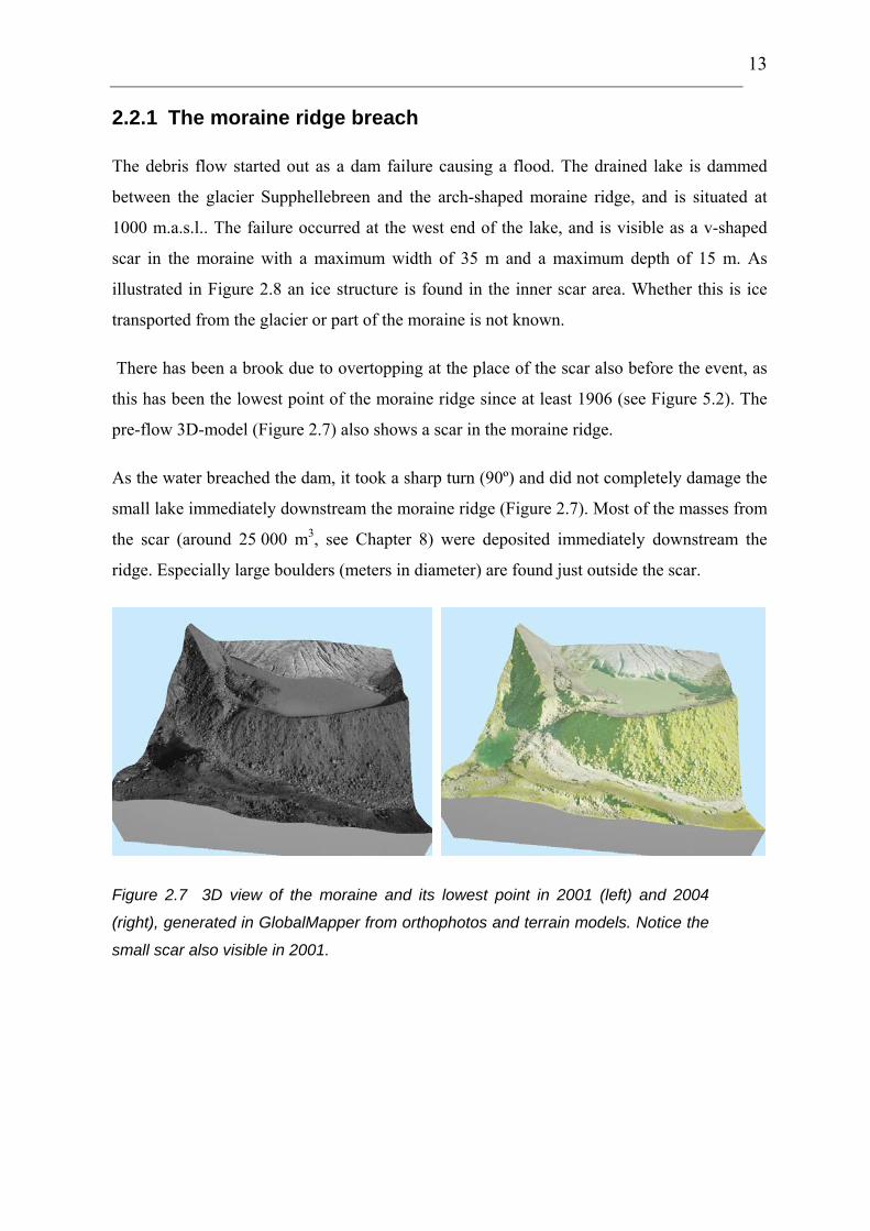
The debris flow started out as a dam failure causing a flood. The drained lake is dammed
between the glacier Supphellebreen and the arch-shaped moraine ridge, and is situated at
1000 m.a.s.l.. The failure occurred at the west end of the lake, and is visible as a v-shaped
scar in the moraine with a maximum width of 35 m and a maximum depth of 15 m. As
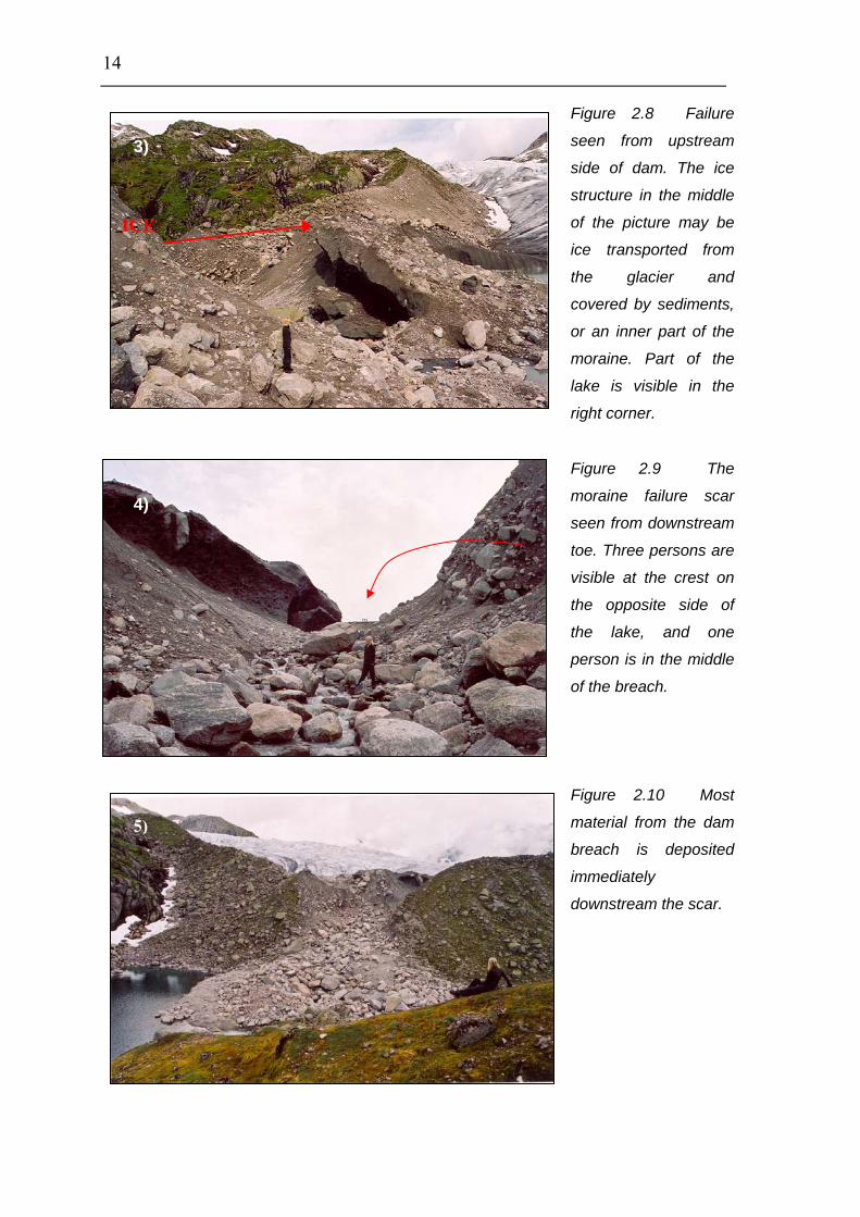
illustrated in Figure 2.8 an ice structure is found in the inner scar area. Whether this is ice
transported from the glacier or part of the moraine is not known.
There has been a brook due to overtopping at the place of the scar also before the event, as
this has been the lowest point of the moraine ridge since at least 1906 (see Figure 5.2). The
pre-flow 3D-model (Figure 2.7) also shows a scar in the moraine ridge.
As the water breached the dam, it took a sharp turn (90º) and did not completely damage the
small lake immediately downstream the moraine ridge (Figure 2.7). Most of the masses from
the scar (around 25 000 m3, see Chapter 8) were deposited immediately downstream the
ridge. Especially large boulders (meters in diameter) are found just outside the scar.
Figure 2.7 3D view of the moraine and its lowest point in 2001 (left) and 2004
(right), generated in GlobalMapper from orthophotos and terrain models. Notice the
small scar also visible in 2001.
14
Figure 2.8 Failure
seen from upstream
side of dam. The ice
structure in the middle
of the picture may be
ice transported from
the glacier and
covered by sediments,
or an inner part of the
moraine. Part of the
lake is visible in the
right corner.
Figure 2.9 The
moraine failure scar
seen from downstream
3)
ICE
4)toe. Three persons are
visible at the crest on
the opposite side of
the lake, and one
person is in the middle
of the breach.
Figure 2.10 Most
material from the dam
breach is deposited
immediately
downstream the scar.
5)

15
2.2.2 Debris flow path
The first stretch (300 m) of the flow path has a very gentle slope, around 4º. The area
includes an active sandur delta downstream the moraine, where progressively finer
sediments are deposited by glacier water. In August 2004 (three months after the event)
there was little evidence of the torrent in this upper section (Figure 2.11). This area was
covered with snow at the time of the event, and the debris masses ran on top of this
snowpack, at least in the early phase. Deposition has occurred, but the stream gully also
seems to be somewhat widened in the area, since some erosion has occurred on the flanks.
b)
)
FiØev
A
ar
te
ve
fo
5 a
gure 2.11 a) Along the first 300 m of the path the masses ran on snow. Photo: E. ygard. b) The same area shows little evidence of the debris flow three months after the ent. Lower part of moraine ridge is seen to the left.
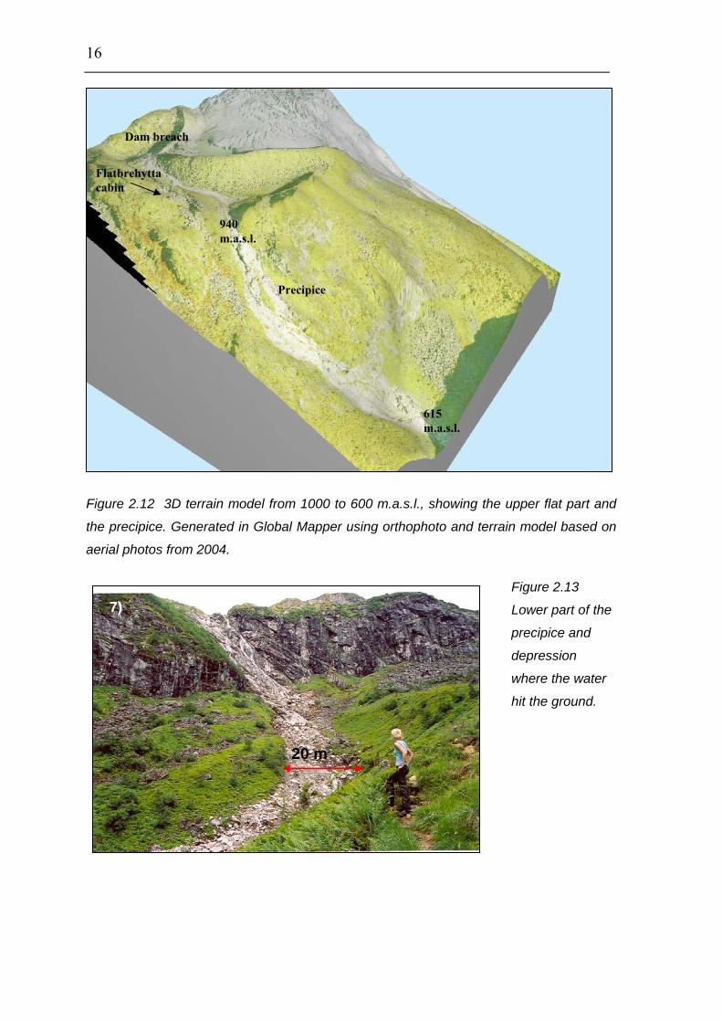
t the precipice 300 m down the path, the masses fell from 900 to 600 m.a.s.l., in a slope of
ound 60º. The area was originally very sparse in sediments due to the steepness of the
rrain and the high altitude. The masses however scoured the precipice, removing all
getation and leaving the bedrock bare in an up to 100 m wide area, as no confining gully
r the masses exists here (see Figure 2.12).
16
Figure 2.12 3D terrain model from 1000 to 600 m.a.s.l., showing the upper flat part and
the precipice. Generated in Global Mapper using orthophoto and terrain model based on
aerial photos from 2004.
Figure 2.13
Lower part of the
precipice and
depression
where the water
hit the ground.
Dam breach
Flatbrehytta cabin
940 m.a.s.l.
Precipice
615 m.a.s.l.
7)
20 m

17
From the point when the water reached the bottom of the precipice at around 615 m.a.s.l., the
loose bed of moraine material starts to thicken, making the erosion potential grow. The large
height drop added momentum and erosive power to the mass. Together this resulted in
deeper erosion where the flow hit the valley, and the gradual formation of a debris flow as
sediment was entrained. The flow can be described as confined all the way to its depositional
fan, as it followed a stream gully. Erosion is obvious from this point on.
The first stretch of Tverrdalen beneath the precipice has a slope of around 23º, but decreases
to approximately 13º after only 150 m. The erosion due to the torrent of water, boulders and
fine sediments produces an average track of around 20 m width and around 1-2 m depth in
this 150 m upper part of the valley. However, this section is characterised by a narrow, deep
erosion channel in the middle of the track. Boulders around 5 m3 observed in the track have
not been moved at all, as only one or two sides of the stones are scoured. Moss and lichen
still growing tell that the stone is the outer limit of the flow (see Figure 2.14). The erosion is
light compared to areas further down the track.
Figure 2.14 The debris flow
has run on top of the stone
as this part is bare, whilst its
side against the camera is
unaffected and covered by
lichen.
8)
The 13º slope soon gets steeper, and approaches 25º for a short stretch. This part also has
experienced deep erosion (around 8 m).
The erosion belt winds down the valley, following the stream gully, but widening it severely.
The width of the track varies considerably throughout the path, widening to up to 53 m and
scouring to a depth of around 8 m. The deepest scour appears in the lower parts of the track,

18
after passing the exit of a smaller tributary stream (see Figure 2.15). The lower parts of the
path are also characterised by being totally scoured, whilst the upper parts are only depleted
in fine material, the coarser seeming to remain in the path.
Figure 2.15 The erosion starts to
get severe after passing the small Breach
The
wit
gul
was
han
in t
The
the
stre
soil
9)
tributary stream in the left of the
picture. Photo: H. Elvehøy.
Cliff
Seveerosi
scoured
h almost
ly has bee
hed out i
ging on th
he valley
debris flo
gully mee
tch, but g
, and also
Lightererosion
re on
gully is changed from a classic v-shaped river gully, to a rectangular depression
vertical sides due to the debris flow. The tourist path on the west side of the
n destroyed by the torrent in some areas, and in others it is in danger of being
n a later rainstorm as it has been undercut by the debris flow and is mainly
e dipping bedrock. Some places the scour has reached bedrock. The till deposit
prior to the event seems to have been of varying thickness (up to around 10 m).
w track tends to be the widest in this upper part of the valley Tverrdalen. After
ts the small tributary stream in Figure 2.15, the path tends to narrow for a short
row deeper. This can be due to the geometry of the terrain, the erodibility of the
due to a possibly higher velocity of the torrent.

19
2.2.3 Soil material
10)
Figure 2.16 The vertical sides of the erosion track are up to 8 m high. The upper red part of the material is the weathered soil.
The soil material as far down the valley as shown in Figure 2.16 seems to be finer grained
till than at higher altitudes, but a high content of large boulders is evident. The deposit is
characterised by a weathered, upper layer up to a few meters thick, and a more coarse-
grained lower layer. Blocks are found throughout the whole profile but seem to be more
concentrated in some areas. The weathered part is seen as the reddish upper few meters of
the profile shown in Figure 2.16. The almost vertical sides of the gully were still standing
when the field investigation was done, three months after the event.
Just before the start of the depositional fan the terrain flattens to 5º (100-150 m.a.s.l.). The
material in this area consists of slide deposits from earlier events. The eroded gully has
revealed layers of such old slide material just above the current fan area (Figure 2.17). Local
residents tell that most of the masses from the latest corresponding debris flow in 1947
stopped in this area.

20
Figure 2.17 Old slide deposit
in eroded gully sides,
2.
Fa
of
w
2.
ha
So
up
as
co
dr
11)
elevation 150 m.a.s.l., most
probably being the 1947-
event. The erosion depth is
here more than 5 meters.
2.4 Deposits along the track
r down the track, large boulders with diameter of around 1-2 m, are found on intact parts
the tourist path just on the west flank of the gully. It is positively known that these stones
ere never in the path before. It is also seen in the photo, taken just after the event (Figure
20) that mud was flowing on the flank during the flow. The depth of the debris flow must
ve been large and filled the gully.
me of the boulders fractured during collisions with other boulders (“exploded”) are found
to 25 m outside the main track near the fan area (Figure 2.19). The position of the rocks
well as its fractures, are very young, pointing towards recent cracking. Other boulders
nsiderably larger (diameter up to 3 m) have been shown to be moved, if not in such a
amatic way, as they are lying over trees just outside the torrent track (see Figure 2.18).

21
Fiscpa
Fi10
12)
gure 2.18 A large boulder has crushed a tree just outside the torrent track. For ale, a camera bag can be seen on the left of the large boulder. Debris flow has ssed in the left part of the picture.
gure 2.19 Recently fractured stone found 20-25 m from main track at elevation 0 m.

22
14)
a)
b)
b)
a)
b)
a)
Figure 2.20 Boulders have been thrown up on the shoulder of the gully from the debris flow. The upper photo is taken a few days after event (photo: E. Loe), the lower three months later. The middle right 3D-figure is made by draping an orthophoto over a terrain model. The letters mark the corresponding boulders in the three pictures.

23
2.2.5 Depositional fan
As the valley opens up and the slope gradually decreases to around 12º, deposition seems to
start.
The depositional fan is drop shaped, 420 m long and 300 m maximum width, with an area of
around 80 000 m2. It consists of boulders, coarse pebble and trunks of trees (Figure 2.22).
The area was covered by 5-10 m high trees before the event. After entraining the trees, the
debris flow filled the lower lying road and parking lot with large boulders of the size of
small cars. The outermost boulder has stopped at the flat farmland almost 450 m from the
beginning of the fan, at 20 m.a.s.l.. One of the largest boulders found ran almost 90 degrees
off the main flow direction and stopped 50 meters from the main fan (see Figure 2.21).
When knowing that the total height drop was 1000 m and the horizontal travel distance 3000
m, the height/travel distance is 0.33. The fan-shaped sedimentation area ranges from
approximately 80-90 m.a.s.l. and ends at around 20 m.a.s.l.. The average slope of the fan
surface is around 8-10 degrees, and the outer flanks approach 4 degrees. The depth of the
deposit has not been measured, but seems to vary from 0.5 m to approximately 5 meters.
Some compaction has occurred. Trees still standing have marks showing that during the flow
the masses were up to 1.5 m thicker than the deposit today (Figure 2.23).
15)
Figure 2.21 Dimensions of largest boulder found. Deposited outside the main fan area.

24
Figure 2.22 The fan area and the farm Øygard seen from the hills on the upstream side
of the fan. The barn of outer Supphella in lower part of the picture. Full line represents
the outer limits of the bouldery fan, stapled line shows the area covered by mud. Photo:
K. Kristensen.
16)
There seems to be a distinct grain size distribution pattern with slope change. All boulders
are deposited in the fan, in a slope of 12º to 4º. The finer material is sedimented on the flat
farmland or transported to sea. Within the fan itself, the most pronounced pattern is vertical
inverse layering (Figure 2.23) where the largest stones are on top (Brazil nut) (see Section
2.4). Where erosion of the fan deposit has exposed profiles, double Brazil nuts (two layers)
are observed, which may indicate two debris pulses (advances) (Figure 2.23). There is
however nothing that indicates a pattern of different sized boulders in high elevation parts of
the fan (80 m.a.s.l.) compared to at the lower parts (20 m.a.s.l.).
There is also a bridging pattern in the deposit. Each bridge ends in a large boulder,
producing a force chain backwards. Five main spurs make up the fan.
Mud
Boulderyfan
Exploded rocks found

25
17)
19)18)
Figure 2.23 Fan deposits in Fjærland. 16) Brazil nut effect. Size of largest boulder in the picture is around 1 m. 17) Brazil nut in two layers may indicate two pulses in the debris flow. 18) The few trees left in the fan are scoured 1.5 m higher than the current deposit.
2.2.6 Mud deposit
The finer fragments sized from sand, silt and clay, were deposited over an area of around
250 000 m2, and had a thickness of up to 50 cm (see Figure 2.24 and Figure 2.1). According
to the farmers, the material turned into a liquid when disturbed even for days after the event.

26
On the farmland where the finest material was deposited, some 5 cm was purposely left
when removing the mud, because of its fertility. Mudlines on the post boxes at Øygardsneset
1 km downstream the fan show the maximum thickness of the mud to be around 50 cm.
50 cm
Figure 2.24 Mudmarks on the postboxes at Øygardsneset show thickness of the mud deposit 1 km downstream the fan. For location see Figure 2.1.
2.3 Description of the Fjærland torrent event using eyewitness statements and field observations
When considering witness observations and degree of erosion, the volume of water released
is suggested to be larger than the volume of the lake behind the moraine dam itself, and
additional water is believed to originate from within the glacier as described in Chapters 5
and 6. As the dam failed and the lake was emptied, water drained from within the glacier.
It is not likely that the flow has had a very high velocity in the beginning of the event, as it
took a sharp turn (90º) and did not damage the small lake immediately downstream the
moraine ridge (see Figure 2.3). Most of the masses from the scar (25 000 m3, see Chapter 8)
were deposited immediately downstream the ridge. This is not consistent with a high flow
velocity. Especially large boulders are found just downstream the scar.
Over this first flat stretch of the track, the masses flowed on top of the snow pack. This, in
combination with the gentle slope reduced the erosive power of the masses. The pictures
taken by E. Øygard (Figure 2.4) show a flow with numerous particles, but the main part of

27
The growing debris flow left behind a deep channel ending in a fan of big boulders in the
As the flow propagated and entrained material, the density of the flow is considered high
As the drainage from the dam breach decreased towards the end of the event, the water lost
Just above the deposition area, the flatter section (approximately 5º) has depleted the energy
As described by witnesses, the debris flow front was 45º steep and composed by boulders.
the material originating from the moraine breach had been deposited prior to this. The
torrent seen in the photos is highly turbulent and carries stones of up to 15 cm diameter, but
the masses mainly acted like a very fluid flood. The 300-m height drop and the accumulation
of momentum when passing the precipice increased the erosive power of the torrent.
Therefore the erosive process is believed to have started at around 600 m.a.s.l.. The
erosional power is believed to increase with time and travel distance, due to the propagating
accumulation of momentum and increasing concentration of sediments entrained.
bottom of the valley. The initial volume of the dam failure is very small compared to the
total volume of the deposit.
(around 1.8 g/cm3) in the lower parts of the track due to the boulders found on the nearby
tourist path at around 200 m.a.s.l. (Figure 2.20). Sediment and water volumes are further
discussed in Chapters 6 and 8. The split stones found 20 m from the track indicate that
blocks of this size and larger were in turbulent suspension or thrown up from the torrent
passing by due to grain collisions, and settling on the flank.
erosional power, resulting then in lower sediment concentration again.
of the masses, but due to high velocity and/or large volume the masses still flowed. This low
slope area is made of old slide deposits, the most recent layers from the event in 1947. As
the flow reached slopes of 12º, the loss of energy has become higher than the input from the
driving forces, resulting in deposition.
The front was around 10 m high as it exited the erosion gully and entered the fan area. The
front was stable until it suddenly collapsed and stopped, building the fan (Figure 2.25).

28
1) 2)
3)
Figure 2.25 Illustration of how the front arrived in Supphelledalen valley and collapsed like a punctured balloon as it reached the lower parts of the fan area. After a sketch by eyewitness Ingvar Supphellen. Photo: C. Harbitz.
2.4 The deposit – Brazil nut effect and bridging
The larger particles in the debris flow of Fjærland ended in a huge fan deposit where the
gully flattens out in the valley of Supphelledalen. The fan shows a pronounced inverse
grading, as is also observed in debris flow deposits by other authors (Remaître et al., 2003 a;
Takahashi, 1991).
The phenomenon has earned much attention in science, as it is important for example in
industry, pharmacy and chemistry (Shinbrot, 2004), and can be seen in simple and daily
examples like in a bag of potatoes - it need not be the seller that on purpose puts the biggest
ones on top. The effect is called the Brazil nut, and refers to the fact that in a box of nuts of
different size and type, the large Brazil nuts rise to the top when shaken. Such granular
segregation was first reported in 1939, and was given the name “Brazil nut problem” in 1987
(Huerta and Ruiz-Súarez, 2004).
There have been several suggestions why this segregation occurs. These include convection,
void filling, arching, inertia and buoyancy. For a further explanation of these terms see
Knight, Jaeger and Nagel (1993) and Huerta and Ruiz-Súarez (2004).

29
It is agreed that the larger the block, the faster it ascends. It is however also observed that
there is a critical diameter above which particles descend, resulting in the reversed Brazil nut
effect.
A certain bridging effect is also found in the fan deposit. Bridging or force chains in a
deposit is a sign of unequal force distribution. Force chains are generated between the grains
in contact, and may evolve in a debris flow containing large clasts like the one in Fjærland.
Stresses are transmitted through this network of particle contacts, and only a fraction of the
particles bear a large proportion of the total load (Mueth, Jaeger and Nagel, 1998). This
pattern is also found behind the largest blocks, with a chain of coarse particles stacked and
locked behind it. Topography and remaining trees may also be a factor in the formation of
bridges. Bridging can also be a result of pulse movement, where the different waves flow in
different directions due to the deposit of the previous waves.
The double Brazil nuts observed are probably formed due to pulsing behaviour and repeated
changes in direction of flow. The deposit shows very high content of boulders, suggesting
that grain-to-grain contact has been an important factor in the dynamics. Bridging pattern is
probably due to this, in combination with the topography and resulting settling of large
boulders in front of each bridge. The force chains are results of contact between grains,
showing that at least a part of the debris was not fully liquefied at all times.
These topics are not treated any further in this thesis, but can be studied in the papers by
among others the above mentioned authors. Both phenomena point towards a strong grain-
to-grain contact working in the dynamics of the flow in Fjærland.
2.5 Total duration
The witness opinion of the total duration of the flow varies from 45 minutes to 2 hours. For
example, Ingebrigt Supphellen says that the fountain of black water at the precipice was
visible for about 2 hours, but with uneven intensity. Ingvar, his son, says that the duration of
the whole event was about one and a half hour, and that as the volume started to reduce, it
reduced quickly. For Eirik Øygard, who was at the cabin Flatbrehytta, the event seemed
faster, and it did not take a long time before he could see the mud at his TV-antenna in his

30
fields. He reports that he heard the slide five minutes to one, and went out to watch the event
10 minutes later. After half an hour there was almost no flow in the river (i.e. 45 minutes).
It has been reported that half an hour passed from the masses first were visible at the
precipice until they reached Supphelledalen. Half an hour for the masses to travel 2 km
seems unlikely, and there is no sign of a temporary basin damming the masses. The most
probable reason is that Ingebrigt Supphellen observed the very beginning of the flow at the
precipice. The first water wave probably had little erosional power, meaning that water
transporting sediment in suspension and by bed-load transport reached Supphelledalen. A
small river would not be visible from Øygardsneset due to the forested fan area. As the
torrent gradually entrained more and more material the front of the debris flow developed,
explaining the time-lag between the first observation of water and the arrival of the debris
flow front.
A scary and dramatic event can seem never to end, but it can also seem to be over in seconds
because people tend not to get time to think. In this case it seems that 45 minutes is the most
appropriate estimate of the main part of the debris flow. It is difficult to determine when the
water flow stopped, since the river was large and sediment-rich for days after the event. This
is seen in pictures taken hours and days later.

31
3. Previous debris flow events in Fjærland
When examining the fan deposit, scoured areas on the flanks have revealed sediments that
probably are old landslide or debris flow deposits (Figure 3.1). Under a layer of soil, stones
and boulders can be found, resembling the deposit of the new fan. According to Eirik
Øygard all the hills in the opening of Tverrdalen (100-150 m.a.s.l.) towards Supphelledalen
are landslide deposits. Also the presence of alders, which are the fastest to recover after a
landslide, indicates unstable times. It should however be noted that snow avalanches are
common in the area.
Figure 3.1
On the flanks of the fan cuts
exposing old slide material are
found. The boulders on top of the
soil are fresh and originate from the
2004 debris flow, whilst the boulders
seen beneath one m of mould were
deposited here in the past.
New slide
deposit
1 m
From new
slide Old slide
deposit
Nearest neighbour upstream the fan area, Per Christian Liseter, has cleaned his fields for
stones and buried the biggest boulders, covering them with soil. During this work fertile
mould has been found, buried under meters of coarser sediment resembling slide material.
When he earlier has reworked other sections of his farmland due to frequent stones and
boulders, similar mould was found.
Ingvar Supphellen living at Øygardsneset 1 km downstream the fan has had large areas
inundated by mud due to the 2004-debris flow. No stones or coarse particles are found in

32
this area, since the stretch from the fan to the farm is almost flat. When digging a trench in
his fields, similar layers of mud were found under a meter of soil. These findings suggest
that similar events may have occurred in the same area before. The mud at Ingvar
Supphellen’s fields has been shown to be very fertile. According to him, it is a fact that there
“always” has been a big difference in the fertility between his farm and Supphella further up
in the valley, an area the debris flow from Tverrdalen does not reach. This may suggest that
something happens here from time to time.
There is historical evidence that similar events have happened twice during the 20th century,
one in 1947 and one in 1924. According to his father Ingebrigt Supphellen, still living in
Supphella, the event dating back to 1947 damaged the bridge over Tverrdøla (near the fan)
and divided the river into two parts. The road was damaged by the flow, but the stones
carried were not as large as in 2004. However, they were big enough that local residents had
to use a stump puller to remove them. Most material was deposited just before the start of
the 2004-fan at elevation 100 m. Ingebrigt Supphellen knows that the reason for the event in
1947 was a moraine ridge failure.
Photos taken before the 2004 debris flow event show a small breach scar in the ridge,
probably dating back to 1947. As seen from Figure 3.2 this was evident in a photo taken
around 1980, but not in the photo from 1906. It seems however that in 1906 this area was
lower than the rest of the ridge, and it almost looks like the glacier had grown in the
direction of the breach area, almost damaging the ridge here.
Figure 3.2 Left: The lowest point of the ridge is seen even in photos from 1906 Photo: Monchton, NGU photo archive. Right: A significant breach is seen. Photo is taken approximately around 1980. Photo: Norsk Bremuseum.

33
A diary written by his neighbour and Eirik Øygard’s grandfather, also called Eirik Øygard,
November 11, 1947, describes this event (see Appendix A). He compares the flow of the
river Tverrdøla to a snow avalanche. The masses were described as black and saturated with
sediments. The diary also tells that the 3 m high flood mitigation structure in Supphelledalen
was overtopped and damaged by the flow. Also the pulsating nature of the debris flow and
the change of direction are described, as well as the ground shaking and the masses
cascading down the precipice at around 900 m.a.s.l..
The locals in Fjærland also report a big slide in the 18th century, and the tale says that the
farm Øygard was abandoned due to this event. It is not known if this was due to fear of new
slides or floods or because the boulders were too big and the volume too large to be
removed, as they had no machines to help them. The name Øygard (which means abandoned
farm) could result from this happening. Old maps show the farm with the name Rødsete. The
name Øygard can however also have its origin from the Black Death as is very common for
farms in Norway. Another explanation to the name can be the meandering glacial river,
forming islands in the landscape, where the farm was built. This is the case in the nearby
valley Jostedalen. Øy means both island and abandoned in Norwegian.
It can be read in the local history book “Fjærland Bygdebok” that Øygard was left
“abandoned during the Black Death or in a later event”. Trygve Mundal, local resident of
Fjærland and the owner of the book, has however his own complete record of the people
living at Øygard dating back to 1616.
In 1900, the houses of the farm Øygard were moved approximately 300 m, from near the
forest down to the flat fields where they are presently located. According to the inhabitants
this was done either due to the fear for snow avalanches or because they were able to
“control the river better than before”. A millhouse on the downstream side of the fan is also
reported to have been rebuilt three times due to avalanches or floods over the last centuries
(Figure 3.3).

34
Figure 3.3 The millhouse has
been rebuilt three times due
to avalache activity. Photo: E.
Loe.
All this indicates that mass flows regularly occur in this valley, and that some of them
originate from the moraine ridge and glacial lake is probable. The events 57 and 80 years
ago were probably not as large as the one in 2004. If a debris flow was the cause of an
abandoning of Øygard, a size of the event similar (or larger) to the 2004-flow may have
occurred. This could mean that a flow of this size or larger has a recurrence interval of 300
years. To get a further understanding of this, dating (C-14 or corresponding) of the deposits
in the area could be carried out.
3.1 Future events
A new debris flow in the future is not unlikely. The scar in the moraine has not reached
bedrock, and sliding from the sides will also gradually fill the scar. If the climate continues
to warm up, melting will fill the lake rapidly, and a new dam failure will probably occur.
The cut-off of drainage channels under/in the glacier (see Chapter 5) is also likely to occur
from time to time. The question is how large a future event will be. Availability of erodible
bed material is often a limiting factor for returning debris flows, and in the Fjærland case
erosion has reached bedrock only a few places. The magnitude of a new event cannot be
determined accurately, but it seems from earlier events that the size of the 2004-event is in
the upper range, and that the present scour of the gully will limit new flows from growing to
the same magnitude. See also Chapter 12.

35
4. Terrain modelling
This section describes the methods used in the photogrammetry process as well as in the
laser scanning, and discusses their reliability. These techniques allow the reconstruction of
3D geometry of post- and pre-flow terrain and 3D change in topography. Multi-temporal air
photos allow for elevation change estimations which can result in debris flow volume
estimates.
4.1 Aerial photos and photogrammetry
The use of vertical aerial photos as a stereo model in terrain modelling requires overlapping
sets of photos. It is necessary that the photos are positioned correctly relative to each other,
and also to the real world. This means that the position of the airplane is required.
First an interior orientation where the pixel coordinates are recalculated into the camera-
coordinate system is performed. There are approximately 20 000 x 20 000 pixels in each
picture, and the camera-coordinate system is in mm. The transformation used is an Affine
transformation, meaning that also form or scale is changed during the transformation.
Second, a relative orientation is needed. This determines how the two pictures are
positioned relative to each other. If at least five points in the two pictures are found to be the
same, there is only one possible relative position. In this case, 10 points were used to
increase accuracy
Third, absolute orientation must be performed. This is done to determine how the pictures
are positioned relative to the actual terrain coordinate system.
4.1.1 Stereo model
This work resulted in pre- and post-event stereo models of the area, the 2001 aerial photos
representing the pre-flow terrain and both the 2004 photos and the laser data represent post-
flow terrain. The stereo models can be used for visualisation and direct measuring, but also
to manually check the terrain models.

36
Problems Given parameters in the photos should match the GPS data from the airplane. It seems that in
this case there are some meters in offset between the coordinate system on the ground and
the one in the GPS data set. The height difference between the GPS data and the control
points in, for instance, corners of houses are large in some places (7.8 m). An offset is
normal, especially when the distance to the GPS reference station is large. This will however
not affect the absolute precision of the coordinates or heights. This can be due to control
point quality and/or that the reference station for the GPS was situated far away. The control
points were taken from coordinate lists and maps.
4.1.2 Orthophotos
An orthophoto can be generated if aerial photos, with known absolute orientation, and a
terrain model are available. The aerial photo is projected on to the terrain, and the result is a
map of x- and y-coordinates with a photo draped on it. This is an image in an orthogonal
(map) projection, and can be used to for example to measure the widening of the gully, but
not the vertical erosion (i.e. 2D). Two orthophoto versions are made in this case, one based
on the photos from 2001, and the second on the 2004 photos.
When making the orthophotos, the terrain elevation from the laser scanning was used both in
combination with the pictures from 2001 and 2004. This is a simplification, but the elevation
error for a point in the picture will be small, as the height to the plane is large (2450 and
3900 m). An orthophoto is two-dimensional (elevation not included) and the horizontal
difference will be minimal.
As this decision was made, it was not known that the laser scanning missed control heights,
which makes these errors larger. The problem of uncertain control heights is further
discussed in Sections 4.2.1.
4.1.3 Digital terrain models
The computation of a terrain model is based on a procedure which identifies and measures
common points in a stereo model by image correlation. The photos are taken from different
directions, and in steep terrain the photos from different angles will look different. Some
37
features may be visible only in one of the pictures, or a boulder may seem not to have the
same form as the angle changes. Visualisation of the terrain models are shown in Figure 4.1
and Figure 4.2.
In this case terrain models from 2004 were to be compared to terrain models from 2001.
Some difficulties related to this comparison were:
• movement of objects in the meantime (stones etc) • vegetation change and growth
• 2004 photos in colour to be compared to 2001 photos in greyscale.
• shadow in parts of the track and in the moraine breach area. Especially colour
photos (2004) turned out to be unclear in these parts.
• 2001 photos taken at inappropriate time of year (summer)
• 2001 photos not especially made for the purpose (shooting angle not optimal)
• 2001 photos taken from higher altitude (3900 m) than the 2004 photos (2450 m).
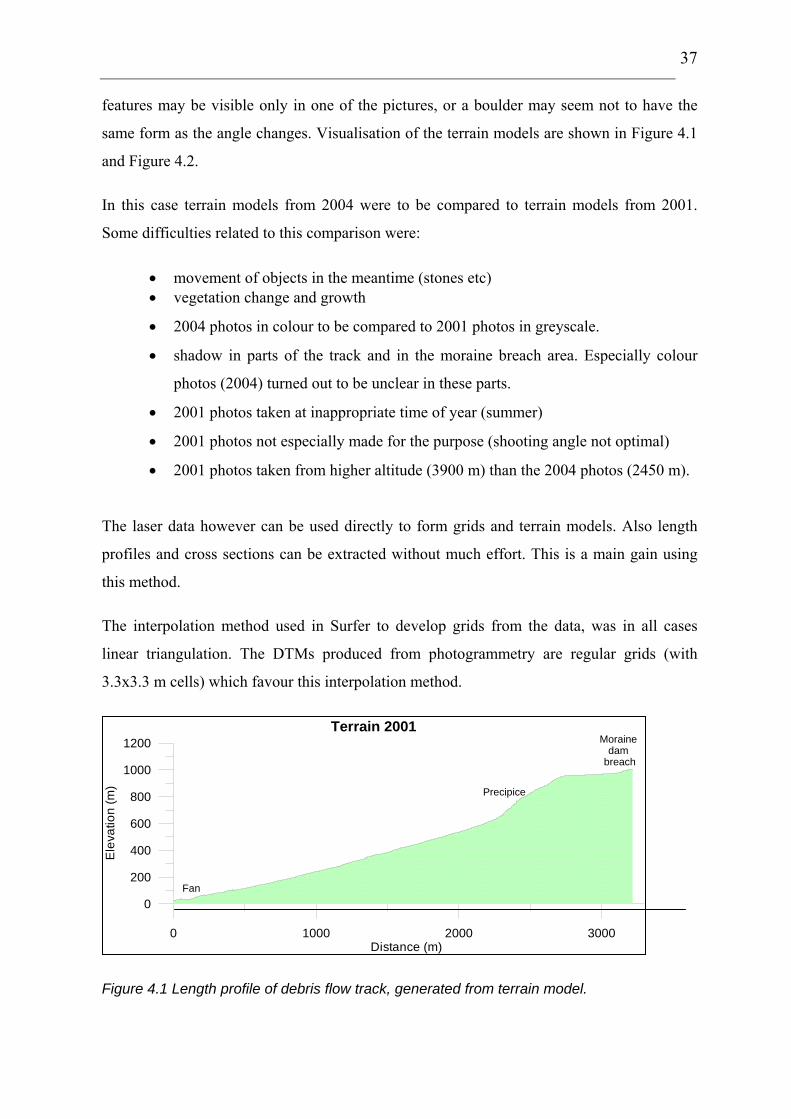
The laser data however can be used directly to form grids and terrain models. Also length
profiles and cross sections can be extracted without much effort. This is a main gain using
this method.
The interpolation method used in Surfer to develop grids from the data, was in all cases
linear triangulation. The DTMs produced from photogrammetry are regular grids (with
3.3x3.3 m cells) which favour this interpolation method.
0 1000 2000 3000
Distance (m)
0
200
400
600
800
1000
1200
Ele
vatio
n (m
)
Terrain 2001
Precipice
Fan
Moraine dam
breach
Figure 4.1 Length profile of debris flow track, generated from terrain model.

38
Figure 4.2 Surface terrain model generated in Surfer.
4.1.4 Resolution
The standard deviation for the stereo models is 6.4 µm, which for the 2004 model
corresponds to approximately 10 cm when using an average scale of 1:15 000. This is found
by:
cmmmmm 1096150000064,0 ≈=⋅ in horizontal direction.
The scale is mostly larger than this, 1:10 000 at the glacier but 1:16 000 in the
Supphelledalen valley.
Corresponding standard deviation for the 2001-model will vary from 12.8 to 16 cm,
dependent on the scale varying from 1:20 000 to 1:25 000.
The pixel resolution is 12 µm in both series from 2004 and 2001; that is, the pixels are 18 on
a 1:15 000 scale and 30 cm on a 1:25 000 scale (at 0 m.a.s.l.), but this will vary with the
terrain altitude. The 2004 pictures have been taken from a lower altitude (2450 – 2480

39
m.a.s.l.) than the pictures taken in 2001 (3900 m.a.s.l.). This means that each pixel is smaller
in the 2004-pictures. The terrain model based on the pictures from 2001 will therefore be
less accurate than the one using the 2004-pictures. Since the flying altitude is more or less
constant above sea level, the biggest uncertainty will occur in the lowest areas (farmland and
fan). Here the height from ground to the airplane is the largest. The variations in resolution
will be relatively large as the elevation variations within the area are pronounced (1000 m).
The vertical precision (height precision) is believed to be 0.06-0.15 ‰ of the flying altitude
in flat terrain, whilst in steep terrain it can drop to 0.9 ‰ (Barstad, 1998). The precision will
be considerably reduced by a higher flying altitude. This means that the precision of all
terrain models must be determined by the pictures taken in 2001 (altitude 3900 m.a.s.l.). The
distance between the plane and ground decreases in higher altitudes, and this must be taken
into account when estimating the uncertainty. This means that the heights are within a range
of 23 cm (0.06 ‰ of (3900-25) m) for the lowest flat areas in Supphelledalen. In the
precipice area the uncertainty may reach 0.9 ‰ of (3900-700) m, which is 2.88 m, and the
flatter areas near the moraine get an uncertainty of around 0.006 ‰ of (3900-1000) m, which
means 17.4 cm. This means an average of around 20 cm.
There is also a minimum limit for cell size in photogrammetry, which is a function of
resolution, camera and flying altitude. The 2001 photos determine the cell size of the grids
generated. In this case the minimum cell size was 3.24 m, and a cell size of 3.333 m was
chosen for all grids, as for comparison the same cell sizes are needed in all the grids. Each
cell gets an averaged value of several pixels. In the generation the points are given different
colours indicating whether the pixels have almost the same value (orange), strongly differing
values (red), or few values (blue). Typically, very steep terrain or hummocky surfaces with
many blocks, get red colour. Especially the precipice from 900 to 600 m.a.s.l. turned out to
be difficult to represent accurately.
As photos from different angles are needed in photogrammetry, steep terrain commonly
creates problems. This is especially the case in the precipice area but also on the east flank
of the stream Tverrdøla due to the steep terrain towards the mountain Vetle Supphellenipa.

40
4.2 LIDAR laser scanning
The laser used was of the type ALTM 2300, a LIDAR (Light Detection and Ranging) laser
scanner. The method is based on distance measurements between the scanning device and
the reflecting object, and precise orientation of the measuring device (Figure 4.3). The laser
sends pulses of beams at regular intervals towards ground, and an oscillating mirror sweeps
the beams in a Z-pattern across the flight path. The ground reflects the laser pulse, and the
time interval between the transmission and the return of the pulse is measured and
transferred into distance. Also the angle of the beam hitting ground is measured. The
strength of the reflected signal varies with the properties of the ground.
The method requires accurate determination of the airplane’s position and orientation (direct
georeference). This is done by GPS and an integrated Inertial Navigations System (INS).
The laser’s position at each pulse admission can be determined, and by observed angles and
distances, positions on ground are found. The GPS reference receiver should be within 20-50
km for accuracy (Turton and Jonas, 2005, Barstad, 2002)). The result is measured points
characterised by x, y, z coordinates.
Figure 4.3 Airborne laser
scanning. Taken from
Hyyppä et al., 2000.

41
Table 4.1 Technical parameters for laser scanning flight in Fjærland
Parameter Performance
Operating altitude 700 m
Speed 75 m/s
Scanner frequency 32 Hz
Laser pulse frequency 33 kHz
Scanning angle 18º
System calibration can be extensive. One common calibration method is to use control areas
of known height and compare these with measured heights. This is believed to remove bias
and systematic errors by moving or tilting the model to fit the control points. This has not
been done in the Fjærland case as discussed in Section 4.2.1 below.
Laser scanning is especially useful in areas covered by forest and in areas of low contrast or
low solar radiation. A laser is not dependent upon daylight or solar radiation, as the laser
itself generates the beams. Compared to classical photogrammetry this is a big advantage.
The laser scanner also has the opportunity to register two or more returns from the same
pulse. This means that in a forest it is possible to measure the elevation of the ground as well
as the elevation of the tree tops, displayed as first and second pulse return. In the Fjærland
project the second pulse represents ground.
4.2.1 Errors
A laser scanning is vulnerable to disturbance. Errors in the GPS measurements (Barstad,
2002) contribute to a large part of the inaccuracy. Variations in the GPS measurements after
initialisation may occur if the airplane is not smooth enough in its turns. The varying
reflecting properties of the ground together with varying angle of the beam will result in
variations in accuracy throughout the area. Also air contamination and humidity may affect
the reflection.

42
The laser “cloud” is dense, but the point density varies along the path, both due to the
variations in terrain and angle, and also because of the variability in overlapping between the
different stretches.
The GPS in the plane can cause absolute offsets in height in the resulting terrain model. As
mentioned, control points with known height can be measured in flat terrain in both ends of
the wanted area. The laser scanning executed in Tverrdalen lacks such calibration, meaning
that although the relative height differences in the model are correct, the model may have to
be tilted or a parallel displacement may have to be made for the heights to be true elevations
above sea level. But, as mentioned, the terrain representation and the relative heights within
the model are correct. The problem arises when the model is to be compared to models
generated from other techniques or at other times, as is the objective in this case. It could be
possible to manually measure several control points (5-6) which are known not to have
moved in both the laser data sets as well as in the 2001 model, and in this way orientate the
laser terrain model correctly for the future.
It turned out that the terrain generated from the laser scanning had lower elevation than if
using aerial photos. That is, laser elevation lines lay above 2004-photo lines in the generated
maps. This offset becomes larger the further down the valley you get. It is small at high
elevations near the moraine ridge.
It seems however that the laser is more correct than the photo generated terrain in the
precipice area. The error is probably due to the steepness of the terrain. The direction or
angle, from which the 2001 photos are shot, may not be ideal for this terrain.
As seen in Figure 4.4, the laser scanning (blue line), which ideally should fit exactly the red
line (aerial photos from 2004) is consequently situated higher. When studying the contours
carefully, it was found that the laser scanning data are not reliable. They are too low in
altitude. In the figure, the blue and the red lines should exactly match and lie above the green
one in the gully due to erosion.
The offset between the control points and the aeroplane GPS data set in the photogrammetry
could be a factor when considering why the laser-generated terrain model does not match the
one generated from aerial photos, as absolute coordinates are used in this comparison.

43
However, the heights do not match when comparing the laser data with the old map,
indicating that this is not the case.
Figure 4.4 Example of contours. Green lines show 2001-contours generated from air photo, red lines 2004-contours from air photo, and blue lines show laser-based contours from 2004. Black arrow indicates direction of debris flow.
The orthophotos have been used to determine profiles (coordinates) along the track to
carefully examine and analyse. The profiles shown in the terrain models from 2004 are
compared to the same profiles from 2001. In this way erosion along the track becomes
visible. As discussed, steep terrain is difficult to represent correctly using both
photogrammetry and laser scanning.
The terrain models do not only offer a visualisation of the event, but when subtracting the
model representing the 2001 terrain from the one representing 2004, using Surfer, negative
values will display erosion, and positive values sedimentation. In this way it is possible to
determine the total volume involved in the debris flow as well as any pattern of erosion or
sedimentation related to physical parameters like slope angle.

44
4.3 Laser vs. aerial photos
4.3.1 Volume estimate
Since it seems that the absolute heights of the model generated by the laser scanning are
lower than the actual terrain, it is most appropriate to use the aerial photos from 2001 in
combination with the aerial photos from 2004, and not the laser scanning, in the volume
estimation. This is discussed in more detail in Chapter 8. Another advantage in relying only
on the aerial photos in the estimation is that two comparable techniques are used in the
generation of the heights. The problems of steep terrain are the same in the two air photo-
models, and the accuracy estimation technique is also the same in both. Since no laser
scanning exists pre-flow, if the 2004-laser scanning was going to be used, it had to be
compared with the model generated from the 2001 aerial photos. The accuracy is of course
not optimal in the models as they are now used, and could be improved by manual effort,
using breaklines along ridges and streams etc.
A height precision of +/- 20 cm and a change in elevation of 2 m will give an anticipated
volume estimate accuracy of 10 % (Chapter 8).
4.3.2 Visualisation using profiles and 3D models
The laser data is suggested to represent the terrain in a better way than the photogrammetry.
The laser data includes more elevation points, and the elevation precision of these points is
better than what the aerial photos give. In addition, the laser has the advantage of looking
vertically downwards. No two positions are required, excluding the problem of view behind
steep terrain.
According to Blom Geomatics, the accuracy expected from a laser scanning is 5 cm; whilst
Hyyppä et al. (2000) claims that this is the accuracy between the data points, and not real
world vertical accuracy. Their experience suggests a standard error of vertical accuracy of
15 cm on flat ground, increasing to 40 cm for slopes of 40º.
After considering this, the laser data are being used when generating profiles and
representing the terrain, because the relative height differences are correct within the model.

45
5. Glaciology and the Supphellebreen glacier
As the debris flow in Fjærland had its origin in a flood from the glacier Supphellebreen,
glaciology and glaciohydrology are important factors in the search for understanding of the
phenomenon. An important task is to determine the water volume released from the lake and
glacier. This can be approached by following glaciological traces, trying to reconstruct the
way of water transport, as well as considering field and eyewitness observations.
The most probable reason for the moraine ridge breach and the additional water volume
from the glacier is a blockage of the glacier’s normal drainage route, and that due to high
melting rates prior to the event self-enlarging channels at the base of the glacier supplied the
lake with water. This chapter attempts to explain the glacier’s capacity to store water and
then suddenly release it. This also highlights the probability of similar happenings in the
future.
5.1 Glaciers in Norway
Norway is among the countries with the largest glaciated areas in Europe (Liestøl, 1989,
Andreassen, Elvehøy and Kjøllmoen, 2004). 2 750 km2 of glaciers constitute around 1 % of
mainland Norway. The Norwegian landscape of mountains and narrow fjords is mainly
formed by glaciers and ice ages, but also the flatter areas of eastern Norway are formed by
glaciers. Today most of mainland Norway’s glaciers are situated in Western Norway.
The peak of the glacier extent during the last ice age (Weichsel) occurred 18 000-20 000
years ago (Nesje, 1995). After Weichsel ice age the climate warmed and the ice retreated.
The Holocene period dates from 9000 years ago until present. In the beginning of Holocene,
most or all of the ice disappeared. New glaciers were formed in higher mountainous areas
when the climate cooled approximately 5000 years ago (Nesje, 1995), and most of today’s
glaciers are remnants from this period. These glaciers experienced their maximum extent in
1750 (Jørgensen et al., 1997).
Until 1930, the climate remained relatively cold. End moraines from 1930 are found several
places, also near the upper and the lower Supphellebreen glaciers. After 1930, the overall

46
trend has been withdrawal of the ice in Norway, although coastal glaciers have experienced
advancement since 1960. As shown in Figure 5.1 below, the growth of Supphellebreen has
been pronounced. Since 2001 most glaciers have experienced a mass deficit (NVE, 2005).
This may be a result of both low winter precipitation during 2001 and 2003, and high degree
of summer melting in 2002 and 2003.
Figure 5.1
Cumulative net balance
for some Norwegian
glaciers showing that
coastal glaciers have
been growing whilst
inland glaciers have
retreated. Taken from
Liestøl, 1995.
5.2 The glacier Supphellebreen
The glacier Supphellebreen is an arm of Jostedalsbreen, the largest glacier in mainland
Europe (487 km2 (Østrem, 1989)), and is situated in the county of Sogn and Fjordane in
Western Norway. Supphellebreen has an approximate area of 11.8 km2, and its elevation
varies from 1730 to 720 m.a.s.l.. There is also a regenerated glacier part named Trollabyrgje
below this elevation, as a result of ice falling from the snout. This is the lowest glacier in the
hemisphere south of the Arctic circle (Aarseth et al., 1988), ranging from approximately 55
to 600 m.a.s.l..
5.2.1 Characteristics
Supphellebreen has an aspect towards the south, and the main part of the glacier has a length
of 8.4 km in the glacier flow direction. According to NVE (Østrem, 1989), the glacier is
cascading, meaning that it has a rough and steep surface. The danger of icefalls in the snout

47
area is characterised as very large (Østrem, 1989), and the ice has a movement of around 2
meters per day in the ice fall area, which is among the highest velocities in Norway (Norsk
Bremuseum, 2005). 2 million tons of ice break off every year and cascades down to the
lower glacier. Other areas of the glacier are flat; hence the name Flatbreen is used in this
area. This main part (above 1200 m.a.s.l.) is an over-deepened basin, flat or bowl-like in
shape. If the glacier should retreat, a lake could form in this area. The exact topography of
the bed is however not investigated.
Figure 5.2
Supphellebreen anno
1906. Photo taken
towards the moraine and
the Fjærland fjord. No
lake is evident. Photo:
Monchton, NGU photo
archive.
Figure 5.3
Supphellebreen anno
2004. A lake has formed
between the glacier and
the moraine. Failure of
moraine in right end of
the ridge. Normal
drainage route is
towards the left.

48
5.2.2 History
Supphellebreen reached its maximum around 1750 (Orheim, 1968), during the Little Ice
Age. The moraine ridge damming the present lake probably dates back to this period. When
studying the photos from 1906 and 2004 shown above (Figure 5.2 and Figure 5.3), the
withdrawal of the glacier is evident, although periods of growth have been experienced. It is
also clear that the shape of the moraine ridge has not changed much in the last 100 years.
Only the smaller, inner moraine shown in the picture from 2004 could be of newer origin,
probably from around 1930 when the ice had been advancing for some years and started
retreating. The pictures show that already in 1906 the moraine had a lowest point where the
breach is today (lower right corner in the photo).
5.3 Glacier hydrology
Running water in glaciers has mainly two origins (Hambrey, 1994). Surface melting is the
most important one, but additional contribution comes from the snow along the valley sides.
The main transportation route is through channels. Water in temperate glaciers also runs
under the glacier as sheetflow.
Under the surface of the glacier, there are principally two types (Hambrey, 1994). The
Röthlisberger (R-) channels that run entirely through ice can be several meters in diameter
and transport large volumes of water in a short time. The smaller Nye (N-) channels are
eroded into bedrock beneath the glacier, but can also be combined with a R-channel above.
The flood in Fjærland is probably related to flow in R-channels, as it seems to have
developed during a short time. N-channels need more time to form. However, water may
also be transported as a sheetflow under the glacier. This may especially be the case if few
drainage channels have had time to develop.
5.3.1 Formation of a channel
Channels in glaciers are kept open and the size enlarged by the flow of water itself. The
transition of heat from water to ice and the frictional heat generated are responsible for this
process (Nesje, 1995, Paterson, 1994 and Liestøl, 1989). When the pressure from overlying

49
ice exceeds the water pressure the drainage channel will be reduced, proportional to the third
power of the difference.
When the flux increases, the melting of the side walls will also increase. At the same time
the water pressure rises. The result is enlargement of the channel. The size is adjusted to an
average discharge, as the processes are not fast enough to follow rapid variations.
During the winter season small amounts of melt water is produced, resulting in low rates of
flow through the ice. The small degree of water flowing, in combination with deformation of
the ice, closes most of the drainage channels during the winter (Nesje, 1995). As the spring
comes, the drainage passways need time to develop, resulting in storage of melt water and
high water pressure within the ice or at the base of the glacier (Hambrey, 1994).
The time needed for a sufficient R-channel to develop, ranges from a few days to several
weeks (Paterson, 1994), but the larger the channel, the faster the growth due to higher degree
of heat dissipation relative to the area of the walls. Water pressure is commonly less in big
channels, making the water drain from the smaller to the larger ones (Liestøl, 1989), again
enhancing the rate of flow. The water flow gradually opens and widens the channels
throughout the summer (Paterson, 1994), resulting in lowering of the basal water pressure
again.
Figure 5.4
Water pressure in the
glacier South Leduc,
Canada, showing higher
average water pressure
during winter than during
summer. The peaks are
associated with storms or
high melting. Taken from
Paterson, 1994.
50
As mentioned, when a drainage system is cut off (Paterson, 1994), water pressure builds up
beneath the ice, partly counteracting the glacier weight and resulting in enhanced glacial
motion. This means that melt water and water pressure determines the rate of basal sliding.
A few millimetres thick layer of water under the ice can increase the glaciers movement with
100 % (Hambrey, 1994). As discussed, Supphellebreen has a rapid movement.
In the days before May 8, 2004, Supphellebreen was observed to be especially active.
Calving and ice falls are results of glacier movement. This movement supports the idea of
high water pressure in and under the ice because of high melting rates and change in
drainage pattern.
5.3.2 Discharge variations
Floods are not uncommon in glacier rivers. These rivers have a discharge pattern (Hambrey,
1994) characterised by extreme diurnal variations and maximum flood during summer.
Figure 5.5 shows how discharge is related to temperature in glacier rivers. They show
pronounced floods every 24 hours where the discharge can be twice the minimum of that
same day. This diurnal pattern is related to the weather condition and the sun's intensity
during the day, melting water rapidly transported through moulins. Also the base-flow
component influences river flow. Base flow is slow in its response and results from water
transported through snow (Paterson, 1994).
This means that water transport through snow is slow, and drainage through ice channels
more rapid. A rapid flood like the Fjærland is likely to be due to a sort of channel drainage,
most probably at the base of the glacier.

51
4-Jul 5-Jul 6-Jul 7-Jul 8-Jul 9-Jul 10-Jul
0
4
8
12
16
Dis
char
ge m
3 /sDischarge in Bøyaelvi m3/sTemperature at Supphellebreen oC
Figure 5.5
Glacier rivers follow diurnal
variations, especially in
summertime, displaying
floods every 24 hours. This
is an example from July
2004 in Fjærland.
The glaciers Bøyabreen and Supphellebreen are neighbouring arms of Jostedalsbreen and
situated at almost the same elevation (see Figure 2.1). They are also of approximately the
same size, so that the discharge measurements in the river of Bøyaelvi can be correlated to
the temperature data from the station at the moraine ridge near Supphellebreen. Also the
Bøyaelvi river shows a high discharge on May 8, meaning that there was a natural flood this
day, probably also from Supphellebreen. A blockage of the drainage channels may have
stopped this flood and forced the water towards the lake. There is no measured data available
from the Supphelleelvi river, nor temperature measurements from Bøyabreen. The
Supphelleelvi river is believed to have a daily discharge slightly smaller than Bøyaelvi.
5.3.3 Storage of water
In the beginning of the melting season there is a time lag (Paterson, 1994) between discharge
peaks and melting peaks in glaciers. This period diminishes throughout the melting season;
probably as a result of the development of drainage channels and the reduction in snow
cover; meaning that the drainage rate rises. Normally, from July to August, which is the
period of maximum runoff in glacier rivers, the discharge is higher than the melting. This
means that water must have been stored in the glacier during the early months of summer

52
and later released. Other evidences of a glacier’s capacity of storing water are found in the
literature. Paterson (1994) mentions examples of glaciers releasing up to 38 % more water
during the entire summer than the measured ablation during the same period.
Sudden floods unrelated to weather conditions have been observed by Mathews on the
Athabasca glacier (Paterson, 1994), where there are no visible ice-dammed lakes. This
means that the water must have come from within the ice. Also drilling and tunnelling in
glaciers have uncovered cavities at great depths. According to Paterson (1994) these holes
must be filled with water in order not to be closed by the ice. Some glaciers have also been
observed to heave half a meter in the beginning of the melting season, believed to be a result
of higher water pressure and water-filled cavities at the bed of the ice.
Together with sudden floods and glacial movement, all this supports the idea that water may
be stored in cavities or lakes under or within the ice of a glacier.
5.4 Glacial lakes and Jøkulhlaups
Lakes can be dammed by glaciers in several ways (Hambrey, 1994);
• at the surface of the glacier (supraglacial) • within the ice (englacial) • under the glacier (subglacial) • at the end of the glacier (proglacial)
The latter is the case at the glacier Supphellebreen in Fjærland, the lake growing as the
glacier retreats.
Such ice-dammed lakes are often filled during the melting season of the glacier, and in many
cases more or less regularly emptied by outburst floods, so called jøkulhlaups or Glacial
Lake Outburst Floods (GLOF) through channels or under the ice.
Jøkulhlaups may occur regularly or be more unexpected. The frequency of the floods is often
regulated by the variations in glacier thickness, retreat or growth. According to Paterson
(1994), most jøkulhlaups occur at the end of summer or early autumn (July and August), as a
result of the melt-water filling of the lake, but there are examples of late outbursts, like the
53
jøkulhlaup from Østerdalsisen in October, 1945 (Liestøl, 1956). The last similar flood from
Supphellebreen through Tverrdalen valley occured in November, 1947.
Jøkulhlaup hydrographs show pronounced peaks. These sudden outburst floods can be
extreme, and discharges of 50 000 m3/s have been recorded in outburst floods from
Grimsvötn in Iceland (Paterson, 1994). Grimsvötn is one of the best known lakes
experiencing regular outburst floods. Another famous glacier dammed lake was the ice-age
lake Lake Agazi in Canada, with a size of over 200 000 km2.
5.5 History of Supphellebreen lake drainage
According to Aarseth et al. (1988) the moraine- and glacier dammed lake at Supphellebreen
fills each spring, and drains through drainage channels beneath the ice towards Supphellen
during summer/autumn (Figure 5.6 and Figure 6.5). The drainage used to occur in August or
September in the 1960s, but when the report was written (1988) this time had changed to
July, probably as a result of thinning of the glacier (Aarseth et al., 1988). This can have two
origins; the melting rate causing faster filling of the lake, as well as the lower pressure of a
thinner glacier making it easier to develop drainage tunnels under the ice or uplift it. Aarseth
et al. (1988) stated that the normal drainage pattern of the lake is a jøkulhlaup (glacial lake
outburst flood (GLOF)), the drainage occurring over a time period of hours. The jøkulhlaup
normally has direction towards Supphellen, through the icefall. The flood of 2004 took the
opposite direction, through the moraine (Figure 5.6).
Also Orheim (1968) writes that the glacier dammed lake is regularly drained each autumn
under the regenerated glacier and down to Supphellen. As seen from Figure 5.6, the lake can
be completely emptied by these jøkulhlaups.
These drainage tunnels are cut off before each spring. According to Orheim one can
determine the start of the melting season by the water level in the lake. He states that as a
rule there is very little ablation before the end of May, and that the melting water generated
before this typically refreeze in the snow. According to Nesje (1995), the ablation season in
Norway usually ranges from May 1 to September 30.

54
2004-drainage
Normal drainage route
a) a
Figure 5.6 The moraine- and glacier-dammed lake usually drains through the ice towards the icefall in Supphellen every summer/autumn. The drainage channel of 1988 is here seen from the inside of the lake, and the letter a marks the position of the channel. The lake is completely emptied. Photo: J. O. Hagen.
This shows that the ice near the lake and the icefall towards Supphella is in continuous
change, and that drainage channels are opened and closed each year. The opening of a
drainage channel towards the icefall is necessary to empty the lake. If the melting rate is
high and no such drainage channel develops, a breach of the moraine may be the outcome.
According to locals, this happened both in 1947 and around 1920, and the tale tells about
similar and very severe flow in the 1700’s making the inhabitants leave Øygard.
There is also a possibility that the lake was not drained during the summer/autumn of 2003
(suggested by locals), meaning that the lake already stored unusual large amounts of water
before the melting season of 2004 started.
It should be noted that only parts of the glacial melt-water usually enters the lake. The river
Supphelleelvi has its origin at the glacier tongue in Supphella and flows all season in
accordance to the discharge variations of glacial rivers described earlier.

55
6. Estimated water volume involved in the flow
The water volume involved in the debris flow is not known, but has a crucial role in the
dynamics of the torrent since it influences mass flow parameters like yield strength,
viscosity, density, velocity and thereby the erosional power and the run-out length. An
estimation of the water volume involved is made considering the glacial lake area, total
drainage area, temperature, witness observations and cross sections throughout the erosion
track. Sediment volume is treated in Chapter 8.
6.1 Glacial lake area
The glacial lake area was measured to 8750 m2 in the 2001-photos. When compared to the
aerial photos taken after the event in 2004, it is seen that the shape of the lake has changed,
and that the lake level has decreased (refer to Figure 6.1 and Figure 6.2). This is partly due
to the fact that the glacier has retreated between 5 and 15 m over the three years, releasing
new area to be covered by melt-water. The retreat of the glacier is also evident along the
moraine ridge southeast of the lake. It must be noted that the 2004-aerial photos were shot
late September, almost 5 months after the water release, and should not be taken as
accurately representing the actual lake immediately after the breach.
The existence of the lake itself is a result of glacier retreat. A further withdrawal will change
the shape of the lake, as well as the larger area available would decrease the water level if
the water volume stayed constant. A retreat of the glacier however means a higher degree of
melting.
The 2001 picture seems not to show a totally filled-up lake, and there is no significant
stream over the moraine ridge. The orthophoto combined with the terrain model from 2001
indicates that the lake level could increase with 2 to 3 meters before any overflow would
occur. From the aerial photos taken in September 2004, it is seen that the lake area was 7280
m2. This means that the area of the lake has decreased from August 2001 to September 2004.
An additional lake area could possibly be found beneath the glacier snout, meaning that the
thin snout could be floating, and hide parts of the lake.

56
?
Figure 6.1 The moraine, glacRed stapled line illustrates thefrom the air. Photo: Fotonor.
Figure 6.2 After the emptyingglacier snout in 2001 and bluePhoto: Blom Geomatics.
ial lake and glacier snout seen from the air in 2001. possibility of the lake having larger area than seen
of the lake, 30 September, 2004. Red line indicates line indicates extent of glacial lake in August 2001.

57
The glacial lake probably had a surface of approximately 10 000 m2 when the moraine
failure occurred, due to the filling of the lake. Possible additional lake area beneath the snout
is not taken into account in this estimate. According to NVE the water level sank around 5 m
during the event 8 May, 2004 (Elvehøy, 2005). A shoreline in the snow was recognised a
few days after the event, showing the original lake level approximately 5 m above the
surface of the lake (refer to Figure 6.3 and Figure 6.4). The drained volume of the lake is
then estimated to 50 000 m2.
Figure 6.3
The moraine ridge from
its inside, the arrow
showing the former water
level of the ice covered
lake. Photo: Elvehøy,
NVE.
Figure 6.4
Lake level line seen a few
days after the drainage.
Photo: E. Loe.
Moraine ridge Breach
Pre-flow
lake level
5 m
Drainage

58
6.2 Additional water from the glacier
Due to the fact that the moraine failed and the amount of sediment eroded in Tverrdalen,
more than the 50 000 m3 of lake water may have escaped through the scar in the moraine.
The additional water must have come from a sub- or englacial lake formed due to early
melting and cut-off of the normal drainage channels, or due to opening of new channels
emptying a usually closed sub-/englacial lake. The normal route for most of the glacial
meltwater is through the icefall and the regenerated glacier down to the river Supphelleelvi.
This is also the route for the regular jøkulhlaups from the lake. In addition to the fast motion
of the glacier, the observed glacier retreat could possibly be a factor in a change of the canal
system, as the ice is relatively thin in the passage area over to Supphellen.
Figure 6.5
Map of the area. Stapled blue arrow
indicates normal drainage route, red line
indicates cut-off of drainage channels
and full black arrow indicates debris flow
route.
Cut-off ?
Normal
drainage route
Flood
route
The idea is supported by the observation of scars and sediment rich ice in the upper end of
the lake just after the flood 8 May, 2004 (see Figure 6.6). This is interpreted as the outlet of
a glacial tunnel that suddenly drained stored water from the glacier towards the lake due to
the high pressure developed at the base of the glacier. It seems that the water has entered the
lake under its ice cover (maybe at the base of the glacier), vertically lifting the ice sheet, as
the ice on the lake was still intact after the event. This is seen in pictures taken by NVE from
a helicopter three days after the flow. If the water drained through the breach with the same

59
speed as the additional water was supplied from the glacier, an uplift of the ice was not
necessary. Another possibility could be that the lake extended under the glacier, and that a
collapse of the glacier ice in the above mentioned scar region (for example due to thinning)
caused a flood wave.
Figure 6.6 Outlet of glacial tunnel is seen as dark sinkholes and scars in
the glacier. Photo: Elvehøy, 2004.
Moraine ridge
Glacier Lake
Breac
Tunnel
outlet ?
6.2.1 Temperature and melting
The weather was relatively warm during the days before the event, with a sharp temperature
peak starting May 5, approaching the highest temperature May 7, the day before the moraine
breach. This also coincides with a significant peak in discharge in the river Bøyaelvi,
originating from the neighbouring glacier Bøyabreen (see Chapter 5.3.2). If the drainage
route through Trollabyrgje was blocked, this melt-water from Supphellebreen had to be
stored in the glacier or the lake.
It was not noticed by the local residents whether the discharge in Supphelleelvi was
abnormal in the period prior to May 8. If the drainage path was blocked, the river would
have been smaller than normal, but possibly not noticeable as far down the valley as where
the farms are situated. Supphelleelvi also gets water input from smaller creeks draining

60
towards it (Figure 6.5). As this happened in early May, a high temperature would cause
melting also in nearby snow covered areas, resulting in high river discharge. In that way the
absence of drainage from the glacier may not be noticable. Ingebrigt Supphellen living at the
innermost farm in Supphelledalen reports that in November 1947, when a similar but smaller
event occurred, an unusual low level of Supphelleelvi river was observed. This could
possibly be explained by the late date of the event. The drainage path could have been
blocked off for the whole summer, but the lack of discharge was not noticed before the
melting period from other areas was over.
3-Apr 8-Apr 13-Apr 18-Apr 23-Apr 28-Apr 3-May 8-May 13-May 18-MayDate
-5
0
5
10
15
20
Dis
char
ge m
3 /s
Discharge m3/sTemperature oC
-5
0
5
10
15
20
Tem
pera
ture
oC
GLOF/MORAINEBREACH
Figure 6.7 Correlation between temperature at Supphellebreen 1000 m.a.s.l. and
discharge in Bøyaelvi.
The amount of water coming from the glacier is unknown. The warm weather, approaching
10º C at the weather station on the moraine ridge (1000 m.a.s.l.), has melted snow and ice on
the glacier estimated to be 250 mm at 1200 m.a.s.l., 125 mm at 1400 m, and 50 mm at 1600
m (Elvehøy/NVE, 2005) during the few warm days before the event. To use this in an
estimate of added volume of water, the drainage area of the glacier Supphellebreen must be
known.
61
The terrain above 1200 m.a.s.l. is flat or bowl-like (Østrem, 1989). This makes a natural
isolation or cut-off of the drainage, encouraging the theory of blockage of meltwater from a
large area, possibly the whole part of the glacier situated above 1200 m.a.s.l. (approximately
10 km2). According to calculations done by NVE, this makes the maximum water volume
stored in the glacier to be 500 000 m3 at the date of the flood. How much of this (if any) has
been blocked off and released to the lake is unknown. The area could be varied with a factor
of 10 or possibly more, from around 1 to 11.8 km2, which is the total drainage area of
Supphellebreen (NVE, 1988). Also precipitation may have contributed with additional
water.
The theory of the channel-opening process and the movement of the glacier described in
Chapter 5 could mean that the Fjærland flood started during the days or hours before the
breach of the moraine dam, as a small channel started to fill the lake with melt-water,
exponentially increasing the size of the tunnel and the volume of water draining through.
Blockage of tunnels could be due to the fact that spring came early this year, causing higher
degree of melting earlier in the season, before the tunnels were sufficiently opened to
transport the required amounts of water towards the ice fall. Another possibility is that the
lake level was unusually high already before the melting process started.
6.3 Estimated water volume considering cross sections
In an attempt to estimate the maximum cross sectional area available for water flow, profiles
of the eroded gully were studied. The laser scanning has been used when creating the cross
sections. The systematic error due to the lack of control heights does not influence the result
in this case as no comparison is made with the 2001-data (see Section 4.2). All cross sections
can be found in Appendix B.

62
Figure 6.8
Cross sections 1-20 shown on
aerial photos from 2004.
2 1 3
4 19
20 5
6 7
8
9
10
11
12
13
14 15
16
17 18
It must be remembered that only towards the very end of the event, the cross sections
approached the depths suggested in the figures. As the path most probably was continuously
eroded, the scenarios evaluated are artificial.
The investigation indicates that the water volume was not evenly distributed throughout the
event. Both jøkulhlaup- and dam breach hydrographs commonly show a pronounced peak.
The reader is directed to the work of Courivaud et al. (2004) for further information on dam
breach hydrographs. Eyewitnesses in the valley Supphelledalen observed highest intensity in
the beginning and also that the masses came in pulses. Water probably also flowed for some
time before any significant amount of sediment was eroded. Therefore, the average
velocities and the discharge obtained are probably not very representative for the event, but
some estimates are presented below.

63
6.3.1 Scenarios
As the uncertainties are large, different scenarios have been assumed in the search for the
most likely sediment/water ratio; the water volume ranging from 50 000 m3 (only lake
volume) to 550 000 m3 (lake + max. additional water) and a sediment volume from around
100 000 m3 to 450 000 m3 (see Chapter 8).
The first cross section evaluated is the scar in the moraine. The area available is estimated to
394 m2. As the lake level could not approach 1000 m.a.s.l. (level of moraine crest) due to the
existence of a depression in the ridge (997 m.a.s.l.), the water could not fill the whole cross
section. The lake level seemed to decrease 5 m during the event. The bottom of the scar is
eroded down to 992 m. As the surface of a water table is horizontal, the cross section
available is calculated to 90 m2. This is tried illustrated in the sketch in Figure 6.9. The
smallest cross section available is however the one that could limit the water volume.
A time of 45 minutes is chosen in the below calculations, based on judgement of witness
statements.
1000 m
990 m
980 m 40 m 20 m
Figure 6.9 Illustration of scar, stapled line represents pre-flow terrain.
For the smallest water volume considered (50 000 m3), if the water flow was continuous
throughout 45 minutes, the average velocity of the water through the scar in the moraine
(profile 1) can be calculated as follows:
( ) ( )( ) ( )
3 2water volume m area mvelocity m s
time s= (6.1)

64
hkmsms
mm /72.0/2.02700
5.9150000 23
==
The 50 000 m3 does not include the solid masses from the moraine scar material itself. This
could illustrate the case if the masses slid out fast, leaving only water flowing through.
( )( )
3 3350000 18.5
2700
volume m m m stime s s
= = (6.2)
A volume of 50 000 m3 over 45 minutes gives an average discharge of 18.5 m3/s. Distributed
over 2 hours however, this volume p
most likely last
for a longer time than the debris flow and peak discharge, as reported by locals and
roduces an average discharge of 7 m3/s.
The largest water volume considered is 500 000 m3, which would give 200 m3/s discharge
throughout 45 minutes and 70 m3/s throughout 2 hours. The water flow did
photographers. This also means that the peak discharge most probably has been larger than
suggested above.
0 10 20Horizontal distance (m)
30
138
140
142
144
146
148
Ele
vatio
n (m
)
PROFILE 13
Figure 6.10 Cross section 13.
The measurements show that some of the largest cross sectional areas, far down the track, 2 are cross sections near the fan, also almost all the volume of
eroded material should be added to the flow. The largest volume expected to flow through
are around 140 m . Since these
this cross section is therefore 500 000 m3 of water + 450 000 m3 soil (see Chapter 6) making
up 950 000 m3 wet debris. Making the same assumptions as in the previous example, the
average discharge through this maximal cross section is calculated to 350 m3/s throughout
45 minutes.

65
These considerations show that there is space enough for all scenarios (from 50 000 to
e than assumed
above, if not the erosion was in proportion to the masses flowing, so that it all the time
d the
expected density of the debris flow, it will be shown that the most probable water volume
Different volume scenarios and velocities are shown in Appendix C and the 20 profiles can
be found in Appendix B. The sediment estimates are presented in Chapter 8.
500 000) to occur if the channel bed had been eroded before the masses started to flow –
which did not happen. This means that there was probably much less spac
would be room enough for the masses. The low velocities obtained, compared to witness
observations of 50 km/h, are average velocities calculated assuming that the bed was
maximally eroded before the event. The actual velocities were most probably higher.
The volume of 950 000 m3 is much more than expected volume, the chapter on sediment
volume discusses this and limits the range of volumes. The water volume is difficult to
determine, but when also considering the geometry of the scar, the degree of erosion an
involved is set to 100 000 m3 (Chapters 7 and 8).

66
7. The moraine ridge breach
Floods due to failure of moraine ridges may evolve into debris flows relatively fast because
of entrainment of material downstream. These debris flows often run for tens of kilometres
due to the large water volume. Himalaya is probably the area most prone to this type of
events. United Nations Environment Programme (UNEP, 2002) has recently reported that 24
glacial lakes in Bhutan and 20 in Nepal are potential sources of GLOFs and resulting far-
reaching debris flows. But also man-made dams may fail, making the problem of a large
water volume release and subsequent erosion an important problem in all kinds of
environment.
Moraine ridges are commonly steep (up to 40º) and high, and comparable to constructed
dams. Most natural moraine ridges have been stable for hundreds and thousands of years, but
the probability of failure may grow as a result of climate change. This is due to ice
avalanches into the dam, high overflow during storms and melting of ice cores (Clague and
Evans, 2000).
Generally, there are different mechanisms that can cause a ridge failure (Clague and Evans,
2000):
• Overtopping due to ice or rock avalanche into lake, earthquake or extreme
meteorological conditions, causing severe erosion of moraine unless it is
armoured by coarse material. The cohesion of moraine sediments is often low.
• Internal erosion (piping) gradually weakens the dam. The actual sediment in the
dam determines the internal erosion factor. These vary between 3 and 10, and a
value above 5 indicates susceptibility for piping
• Melting of ice core or interstitial ice
• Earthquake causing collapse of dam
7.1 Ridge failure
The failure of the moraine ridge damming the glacial lake is the cause of the debris flow in
Fjærland. The reason for the dam breach is however not so clear.

67
As suggested in Chapter 5 on glaciohydrology, early melting may be the background of the
flood. A gradual rise in the water table of the moraine dammed lake may have overtopped
the moraine and led to erosion, or internal piping may have become enhanced. Another
possibility is that the ridge for some reason simply could not stand the pressure of the water
due to high water level combined with weakening of the moraine.
7.1.1 Failure mechanisms
The failure of the ridge may have started out as a small lowering of the ridge, rapidly
growing with time. This is seen in a series of large scale dam failure experiments done by
Høeg, Løvoll and Vaskinn (2004). An overtopping of a man-made embankment dam of
rockfill with a moraine core resulted in a total dam failure, the breach developing in 2 hours.
They conclude that overtopping first leads to slow dam toe erosion, but as soon as the scour
reaches the upstream crest of the dam, the damage of the dam is rapid.
Internal erosion may also fail a dam. The top flow line through an earthen dam may, due to
a developed leak, emerge at the downstream surface, and gradually erode the face in a
channel-like structure. This process is called piping and was tested by Høeg et al. (2004).
They found that it took a long time to develop a total failure by piping. First when the tunnel
widening reached the crest of the dam, breaching took place.
In the headcut process as described by Høeg et al. (2004) erosion grows upwards towards the
crest, eventually causing failure. As erosion is largest in the lowest parts of the dam,
undercutting leads to faster opening of the breach. Headcutting is most common in cohesive
materials (Courivaud, Lempérière and Fry, 2004), due to the capillary forces and the
characteristic steep slopes of such materials. A noncohesive material would most probably
slide out, and a headcutting process would not occur. Erosion starting at the crest working its
way to the ground foundation is a common failure mechanism due to overtopping in
noncohesive materials (Courivaud, Lempérière and Fry (2004)).
For dam failures removal of lateral and/or underlying support are also important in creating
increased shear stress. This results in periodical failures of the side slopes, for instance in a
failure scar that is developing. At the time of side slope failure, tests have shown significant
drop in soil-moisture tension, and therefore loss of shear strength.

68
7.1.2 The breaching process
Two separate stages may be recognised in a failure process (CD, 2004; Courivaud et al.,
2004, Høeg et al., 2004)). The process starts out with a deepening of the breach until ground,
or equivalent, is reached, shaping the scar more or less into a V-form. The following
widening stage laterally enlarges the scar to a trapezoidal form with almost vertical sides
(Figure 7.1). Rockfill dams, clayfill, gravel and moraine dams all produced almost vertical
scar sides in the tests by Høeg et al. (2004).
Franca, Braunschweig and Almeida (2004) have experienced that the initial width of the scar
is the same as the dam height, the final average width around 1.7 times this, and the final
breach depth 80 % of the dam height. In Fjærland the height from the crest to the ground in
this section of the dam is around 25 m. According to the theory of Franca et al., the final
breach width should be 1.7 times 25 m, which means 42.5 m. The breach width in Fjærland
is around 35 m, which could indicate that the process stopped (Figure 7.1).
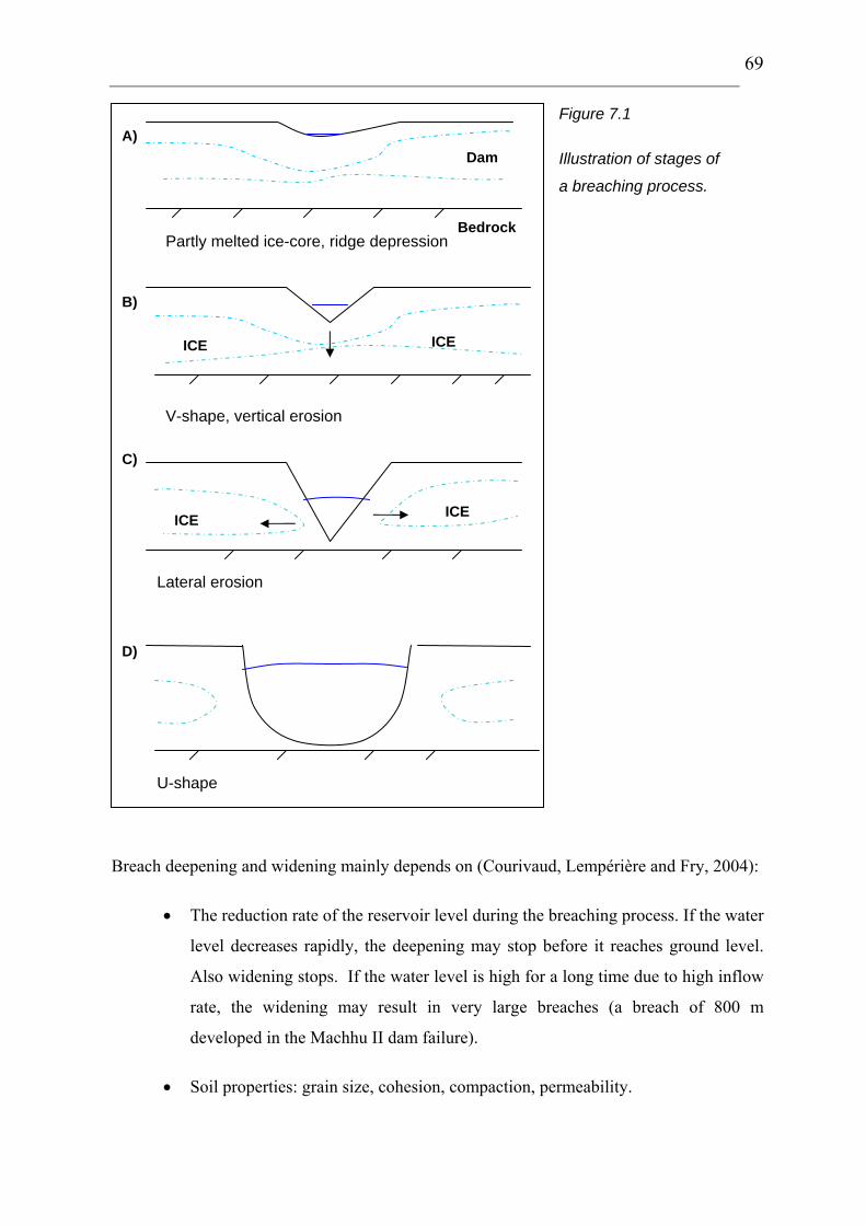
69
Figure 7.1
Illustration of stages of
a breaching process.
Breach deepening and widening mainly depends on (Courivaud, Lempérière and Fry, 2004):
• The reduction rate of the reservoir level during the breaching process. If the water
level decreases rapidly, the deepening may stop before it reaches ground level.
Also widening stops. If the water level is high for a long time due to high inflow
rate, the widening may result in very large breaches (a breach of 800 m
developed in the Machhu II dam failure).
• Soil properties: grain size, cohesion, compaction, permeability.
ICEICE
ICEICE
A)
B)
C)
V-shape, vertical erosion
Lateral erosion
U-shape
Dam
Bedrock Partly melted ice-core, ridge depression
D)

70
In a dam constructed by cohesive material, the widening of the breach will be slow. The
progression (Courivaud, Lempérière, Fry, 2004) may be considerably faster and the breach
may get wider, if the material is cohesionless and the reservoir level stays high for a long
time.
It seems that the widening process in Fjærland has been stopped before the breach has
reached a full trapezoidal form. Very similar breaches have been observed in enormous
GLOFs from Himalaya (Figure 7.2). This could mean that moraine material dams may
exhibit a larger resistance to breach widening than many other dam types, due to existence of
cohesive clay material and/or ice.
Figure 7.2
Breach of moraine causing
glacial lake outburst flood
and debris flow in high
altitude Nepal. Photo:
Øystein Lund.
Pickert et al. (2004) state that breach widening strongly depends on the soil/water
interactions in the soil matrix. Suction in partly saturated soil increases the strength of the
soil, and may for example influence erodibility and stability of the slope. A material of high
cohesion will be stable also in an almost vertical position due to capillarity. The stabilising
force is based on soil-moisture tension and increases the effective stress and the apparent
cohesion.
Suction changes with rainfall intensity, slope geometry, porosity, degree of saturation, strain
rate and soil properties (Chen, Lee and Shen, 2000). A Coulomb failure criterion will look
like this when suction is taken into account (Lambe, 1996):

71
cppp bwaa ′+−+′−= ϕϕστ tan)(tan)( (7.1)
where
pa = pore air pressure
pw = pore water pressure
φb = friction angle relative to matric suction
The increase in shear strength caused by an increase in matric suction is described by φb.
The resulting increase in strength can be significant. φb normally varies between ½ φ´ and φ´
(Høeg, 2004). When the soil is saturated, we get the classical shear strength relationship as
modified by Terzaghi in 1936. In Fjærland the water content of the dam is believed to be
high due to a melting ice core and/or snow, and moraine material flows easily when exposed
to too much water.
The fact that the breach scar still is quite small is also an indication that the water volume
was in the lower end of the range (50 000 – 500 000 m3) suggested.
7.2 Possible ice core in Fjærland
Whether the moraine ridge in Fjærland is ice-cored is important in the evaluation of the dam
stability, and is not known at this time. A further investigation of the moraine is planned in
June 2005, unfortunately after this thesis work has been terminated. Seismic reflection and
refraction, Ground Penetrating Radar (GPR) and electrical resistivity methods will be used.
The melting of an ice core would strongly reduce the safety factor of the dam. Not only
would the porosity grow larger, but the material would get wet and unstable. The moraine at
Supphellebreen is situated at 1000 m.a.s.l., and this is well below the normal permafrost
limit (1450 m.a.s.l.) in mountain ranges like Jotunheimen in Norway (Meteorological
Institute, 2003). Sporadic permafrost can however be found 300-400 m below this limit, and
according to Norwegian Meteorological Institute very little research has been done in the
western part of Norway on permafrost limits.
As the moraine is in contact with the glacier all year round, as well as with the icy water in
the lake, there is a good chance the moraine is ice cored. The topography makes the moraine

72
exposed to cold winds, and for a thick moraine ridge like this, it would also take a
considerable amount of energy to fully melt an ice core during a short summer.
Internal erosion (piping) may continuously have weakened the moraine in Fjærland if an ice
core has started to melt. This would also enhance the melting process. If the moraine is or
has been partly ice cored, an incipient melting process will start internal erosion. The water
flow will cause ever more ice to melt, which again will force erosion growth. The lower part
of the crest could possibly be a result of such melting, internal erosion causing settlement. In
experiments, and in the field, sinkholes have been observed due to piping. The sinkholes
usually occur on the upstream side of the crest and leads to overtopping (Figure 7.3).
The most probable cause of the local lowering of the crest in Fjærland seems to be erosion
due to previous overtopping. Piping may be the direct cause of the failure, but may also
weaken the material so that erosion due to overtopping gets more efficient. The area
downstream the moraine is wet all year round, indicating such piping.
Figure 7.3 Illustration of different mechanisms possible in a dam with partly melted
ice core. Both overtopping and piping may lead to breaching.
Overtopping Erosion
Piping
ICE
Erosion

73
8. Estimated sediment volume involved in the flow
Ice ages usually remove evidence and sediments of earlier times, therefore the main part of
Norwegian soils and moraines were formed during the last glaciation (Weichsel, 118 000-
9000 years ago) or in the following warmer Holocene (Jørgensen, Sørensen and Haldorsen,
1997). As the soil in Fjærland, like in most parts of Norway, is produced by glaciers,
glaciology has a key role also in the study of the sediments involved in the debris flow. The
material incorporated in the debris flow is mainly glacial sediment: in addition to the
moraine ridge studied, the valley scoured by the torrent is covered by this sediment type.
Some of the material in the lower parts of the valley is however resedimented slide material
as discussed in Section 2.2.3. The first section of this chapter treats the characteristics of till.
8.1 Characteristics of the till
Repeated cycles of moving ice, melting, freezing and incorporation of material result in a till
deposit. Normally, the formations (for example a ridge) is called moraine, whilst the soil
material is called till.
The till cover (Haldorsen, 1983) is thin and discontinuous over large areas of Norway,
especially in the western part, due to glacial net erosion in the steep terrain. This part of
Norway is also mainly covered by erosion resistant bedrock types like Precambrian rocks
(>650 mill. years).
Average till cover in Norway does seldom exceed 5 m. Most of the moraine sediment has
been transported relatively short distances (Jørgensen et al., 1997; Haldorsen, 1983), often
less than 5 km. Leeside valleys often has thicker till, in for example Gudbrandsdalen up to
50 m in thickness. Commonly, tills in mountainous areas are composed by local material,
whilst the cover in valley bottoms is more far-travelled (Haldorsen, 1983).
Till is characterised by poor sorting (Jørgensen et al., 1997, Hambrey, 1994), and is
composed of fragments of all sizes; from clay to boulders due to the different formation
processes like abrasion, melt-freeze and plucking. The various particles can have completely
different rock type origin and can be sharp as well as rounded. Tills in Norway are normally

74
coarse grained tills where clay constitutes less than 10 % of the fine material (< 16 mm) and
gravel between 2 and 16 mm makes up 20-40 %. The boulder fraction is between 30 and 70
% of the total till (Haldorsen, 1983). Grain size distribution data from 3000 Norwegian
moraines show high content of gravel, sand and silt relative to clay (see Figure 8.1)
(Jørgensen et al. (1997). The Fjærland till seems to include very large amounts of boulders,
making a grain size analysis difficult to perform.
Figure 8.1
Grain size distribution of 3000
Norwegian tills. The left maximum in
the figure corresponds to tills
generated from coarse sedimentary
bedrock, whilst the right maximum
displays tills generated from finer
rocks like clayey slates. Boulders are
not included in the figure. Modified
from Jørgensen et al., 1997.
The till composition depends on:
1) Transport:
• sediment transported at the base is crushed into fine, round material.
• sediment transported on top or within remains coarse and sharp.
2) Sediment origin:
• rock type, characterised by shear strength, hardness and degree of fracturing
(Jørgensen et al., 1997). A gabbro is difficult to pluck for the glacier, whilst
granite and sandstone produces huge amounts of blocks and coarse material.
A clayey slate gives clayey till. In general, coarse sedimentary rocks,
sandstones and gneisses give rise to sandy tills ( clay content is genereally
less than 5 %), whilst Cambro-Silurian rocks are crushed to a sediment of
more than 10 % clay (Jørgensen, 1997)

75
• steep terrain and fractured bedrock (common in Western Norway) produces coarse material (Haldorsen, 1983)
• lowland fields produce fine grained sediment (Haldorsen, 1983)
• leeside till is coarser than pushside till
Moraines are seldom homogenous (Jørgensen, 1997). Although the overall pattern is
unsorted material, sorted lenses often occur. The amount of sorted material reflects the
degree of water present in the sedimentation period.
8.2 The till of Fjærland
The Precambrian rocks of Norway are generally composed of gneisses, granites, deformed
sedimentary rocks and volcanic rocks (Aschehoug og Gyldendals Store Norske, 2004). The
Fjærland deposit is therefore suggested to contain a large fraction of sand due to these rock
types, a considerable amount of boulders due to the steep terrain, and little clay. Depending
on whether the material is far-travelled and the direction of ice motion, clay originating from
a belt of Cambro-silurian rocks (545-417 mill. years) south-west of Fjærland (Aschehoug og
Gyldendals Store Norske, 2004) may be found in the deposit. The material at low elevations
is considered more far travelled than the material at higher elevations. The discussion in
Chapter 7 however indicates that a certain amount of clay exists.
The material in Tverrdalen and lower lying Supphelledalen is believed to be basal till and
composed of material deposited under the ice due to pressure-melting and basal shear
(Nesje, 1995, Jørgensen, 1997). This type of sediment (Haldorsen, 1983) is typically
compact, fine-grained and has a smooth surface. The thickness of the deposit in Fjærland
varies with steepness of terrain and altitude.
As discussed, some of the material involved in the 2004-flow are old slide deposits. The area
is also prone to snow avalanches and rock falls supplying the valley with sediments.
8.2.1 Supphellebreen moraine
An advancing glacier pushes material in front of it, resulting in a terminal moraine ridge.
Such a moraine ridge displays the maximum extent of the glacier. Even a glacier that is

76
retreating may push up small ridges in the winter season. These proglacial tills usually
consist of coarse material if they are situated above the marine limit (Haldorsen, 1983).
The moraine ridge at Supphellebreen is a perfectly shaped end moraine. It is approximately
650 m long, shaped like an arch and is around 25-50 m high. The slope is up to 33º on the
downstream side, and 34.5º on the upstream side.
The material of an end moraine is usually coarse and field investigations and photos from
Fjærland support this view. Large boulders are visible, especially on the upstream side since
this side lacks vegetation. Fine material is found between the blocks.
Some water is usually overflowing the lowest ridge point (Figure 2.7) in the melting season,
making up a small stream. There are also indications that more dramatic floods have
occurred here from time to time (see Chapter 3). The reason that the failure became more
severe in May 2004 may be due to the larger amount of water, advanced internal erosion, or
a partly melted ice core.
8.3 Sediment volume estimate
The sediment volume incorporated in the debris flow of Fjærland was estimated using
Golden Software’s Surfer, generating grids of the developed terrain models (see Chapter 2)
and subtracting the pre-flow from the post-flow grids (Figure 8.2). To minimise the error
only the area affected by the torrent plus some meters on each side, were taken into account.
The area outside the track should display zero change. This is however not the case
throughout the whole path, due to inaccuracy of the models and change in vegetation from
2001 to 2004.
For control, the track was divided into 7 sections (Figure 8.3). The smaller the area studied,
and the more homogeneous each area is, the easier it is to figure out the result. For close-up
of all parts and details on calculated sediment change resulting from the aerial photos, laser
and economical map, see Appendix D.

77
Figure 8.2 Erosion and
deposition throughout the
debris flow gully shown on
a 50 m contour map.
Terrain model 2001 minus
terrain model 2004 based
on aerial photos.

78
2
4
6
1
Figure 8.3 Thcontours, sectleft corner is d
3
7
e division 4, sue to bo
5
ion of the debris flow track into 7 sections. Right: example of howing net sedimentation and net erosion. Sedimentation in lower ulders settled or moved a few meters.

79
Table 8.1 Overview of calculated volumes using different terrain models. Section
number can be found in Figure 8.3. Numbers in bold are used in later
considerations. Numbers in italics represent erroneous numbers.
Aerial photos Laser scanning Ec. map 1:5000
Section 2004-2001
Laser 2004-air photo
2001
Air photo 2001 -
ec.map
Area (m2) Volume (m3) Volume (m3) Volume (m3)
1 Moraine scar 4 345 -23 041 -25 778
2 Flat area 11 473 8 526 -11 334
3 (Precipice) 29 308 (22 926) (-62 446) -
4 Beneath precipice 29 043 -48 067 -118 875
5 Tunga 21 879 -70 157 -130 092
6 Tverrdalen 33 018 -103 714 -176 948
7 (Fan) 75 094 (-156 284) (-309 975) 105 532 Total 204 160 (-369 811) (-835 448)
Total (-3 and 7) 129 066 -236 453 -463 027
The areas used in the calculations are somewhat larger than the actual size of the track; this
is seen in the item for total area in the table above (129 066 m2), which is larger than the
measured area of the track (99 900 m2) for the reasons noted above.
8.3.1 Accuracy of the estimate
The terrain modelling method is expected to give a volume accuracy of around +/-10 % in
this case. On the other hand, the lacking control points for the laser data results in terrain
models that are not suitable for multi-temporal comparison (see Section 4.3). For the
photogrammetry-based estimates, considerations about the difficulty of representing steep
terrain must be taken into account. This is especially true for the lower parts of the track,
where the terrain is very steep on one of the sides. This area is also the section with the most
severe erosion. Almost vertical gully sides are observed in lower parts of the track. A
potentially large volume may here be lost (both using photogrammetry and laser) as shown
in Figure 8.4. Where negative values dominate also the flanks of the track, it is suggested
that erosion estimate may be too large (see Appendix D).

80
Plane
3.3 m
Figure 8.4 A potentially large area (volume) may be lost in steep terrain. Example of losses in a gully of vertical sides are here shown in red.
The eroded volume should roughly correspond to the volume of the depositional fan. In
addition, a part of the eroded material travelled further and was deposited on the flat
farmland, whilst some of the finest material was transported to sea and thereby lost.
The disturbed and remoulded sediment will not have the same properties and the same
densities as the undisturbed soil. Therefore the volume of the deposit may not correspond to
the volume eroded, and the generation of a volume budget is therefore difficult. The packing
is most likely less dense in the debris flow deposit than it was originally. As the volume
estimate of the fan is not accurate, I base my discussion on the eroded volume.
8.3.2 Areas not included in the estimate
In the following I will use the volumes estimated through terrain modelling without taking
into account the following areas ( and Table 8.1):
• the cliff from 900 to 600 m.a.s.l. (Section 3)
• the fan area (Section 7)

81
Both sections include errors. The cliff section displays thick deposition (see Table 8.1),
while field investigations and air photos however show erosion of the soil layer and
vegetation leaving the bedrock bare. I consider the exclusion not to affect the result in an
unacceptable way, as there was very little loose sediment in the area.
Due to the fact that the fan area was almost completely covered by trees when the aerial
photos were taken in 2001 (see Figure 8.5), the estimation relying on these photos does not
represent the correct ground elevation change. Due to this forest, the 2001-terrain therefore
seems to lie higher than the 2004-terrain, displaying severe erosion also in the depositional
area (see Table 8.1). Since the erosion process is considered finished as the mass flow enters
the fan area, not to include the fan gives a better approximation of the totally eroded volume.
Figure 8.5 Part of aerial photo displaying the fan area in 2001. Red line indicates the limits of the 2004-fan. The dense forest in the 2001-photo has caused problems in calculating the fan volume. Air photo: Fotonor.

82
Figure 8.6 Part of aerial photo showing the fan in September 2004. Mud inundating the fields is removed. Air photo: Blom Geomatics.
8.3.3 Photogrammetry vs. laser
As previously described, two methods of generating a pre-flow terrain model have been
used. The lack of measured control areas in the laser scanning made this method generate a
lower terrain than expected. This resulted in a large erosion volume estimate (-460 000 m3),
as the extra meter(s) of erosion accumulates through the 3 km long track. When examining
the contours and profiles from 2001, 2004 and the laser scanning (Figure 8.7 and Figure
8.8), there seems to be a systematic error in the laser estimate, largest at low elevations,
lowest at high elevations (see Section 4.2). The error is not necessarily constant over the
whole model, and this makes it difficult to compensate for. Profile 12 shows that the
photogrammetry gave a 2004-terrain that matches well with the 2001-terrain, as the surfaces
approach each other on the sides where no erosion has occurred, whilst the laser scanning
displays lower elevations. For further details about the laser scanning or the
photogrammetry, see Chapter 2.

83
0 20 40 60 80 100Horizontal distance (m)
960
970
980
990
1000
1010
1020E
leva
tion
(m)
2001 aerial photo2004 Laser2004 aerial photo
PROFILE 20
Figure 8.7
Intact moraine ridge at 1000
m.a.s.l.. The offset between
the laser and the aerial photo
is lowest at high altitudes.
0 20 40 60 80Horizontal distance (m)
200
210
220
230
240
Ele
vatio
n (m
)
2001 Aerial photo2004 Laser2004 Aerial photo
PROFILE 12 Figure 8.8
The offset is larger at 200
m.a.s.l. The laser terrain line
should meet the stapled line
on the sides of the gully where
no erosion has occurred. The
red line satisfies this condition.
Preliminary conclusion Based on the foregoing discussion, for volume estimations the laser scanning is not
applicable. Using the aerial photos alone resulted in a total eroded volume of ≈ 240 000 m3.

84
8.4 Estimated sediment volume considering profiles and field observations
8.4.1 Erosion depth
For a check of the volume estimate from Surfer, the erosion depth observed during field
work is considered. The area of the visibly eroded debris flow track, from the moraine scar
at 1000 m.a.s.l. to the upper end of the fan (at 90 m.a.s.l.) is measured to 99 900 ≈ 100 000
m2 in the orthophoto, using Global Mapper. The length of the track is 2 770 ≈ 2 800 m, and
the average width of the track can be calculated to 36 m. Area and length estimations are of
high quality (horizontal accuracy is very good). To check the estimates, manual
measurements of the erosion depth should be done at intervals throughout the track.
When knowing the area of the track, an average erosion may be computed. Average erosion
throughout the track of 1 m would result in an eroded volume of 100 000 m3, whilst 4 m
erosion gives 400 000 m3. The Surfer estimate of ≈ 240 000 m3 corresponds to an average
vertical erosion of 2.4 m over the 100 000 m2. The upper parts (down to approximately 600
m.a.s.l.) did not experience much erosion, partly due to snow cover, partly due to low
sediment concentration in the water, lower velocity and partly because there was little loose
material to scour. The area below the precipice is measured to ≈ 62 200 m2. The volume
estimate of 240 000 m3 distributed only over this area would then give almost 4 m of average
erosion. In addition some material originated from the cliff and the area above, meaning that
average erosion is somewhere between 4 and 2.4 m. Considering the field estimates of
erosion, an average gully deepening of a bit less than 3-4 m seems correct.
All 20 profiles showing erosion may be found in Appendix B. These are derived through the
terrain modelling methods also used for the volume estimation (aerial photos and laser
scanning), and are thus not suitable for cross validation of the erosion depth and volume
estimate. The profiles show eroded cross sections of up to 130 m2. If all cross sections from
beneath the cliff were around 100 m2, the eroded volume would constitute 280 000 m3.
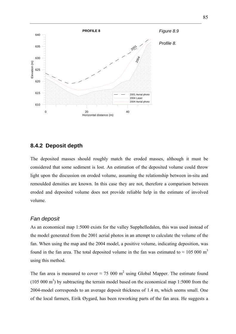
85
0 20 40Horizontal distance (m)
610
615
620
625
630
635
640E
leva
tion
(m)
2001 Aerial photo2004 Laser2004 Aerial photo
PROFILE 8
2001
2004
Figure 8.9
Profile 8.
8.4.2 Deposit depth
The deposited masses should roughly match the eroded masses, although it must be
considered that some sediment is lost. An estimation of the deposited volume could throw
light upon the discussion on eroded volume, assuming the relationship between in-situ and
remoulded densities are known. In this case they are not, therefore a comparison between
eroded and deposited volume does not provide reliable help in the estimate of involved
volume.
Fan deposit As an economical map 1:5000 exists for the valley Supphelledalen, this was used instead of
the model generated from the 2001 aerial photos in an attempt to calculate the volume of the
fan. When using the map and the 2004 model, a positive volume, indicating deposition, was
found in the fan area. The total deposited volume in the fan was estimated to ≈ 105 000 m3
using this method.
The fan area is measured to cover ≈ 75 000 m2 using Global Mapper. The estimate found
(105 000 m3) by subtracting the terrain model based on the economical map 1:5000 from the
2004-model corresponds to an average deposit thickness of 1.4 m, which seems small. One
of the local farmers, Eirik Øygard, has been reworking parts of the fan area. He suggests a

86
fan thickness of approximately 5 to 6 m. This is in the central area of the fan. Towards the
flanks, the thickness clearly decreases.
The fan area has probably been covered by trees for a long time, therefore there may be
errors in the economical map. Due to this, a few attempts to estimate the fan volume are
shown in Table 8.2. The fan is divided into a central area and flank area according to the
figure, and the thicknesses used are average thicknesses of each part.
Figuseenthickof th
5 m
0 m
A B
Central
area
B
A Flanks
Flank 75 m Center 225 m Flank
re 8.10 Illustrations of fan divisions and geometry. Length profile from A to B in aerial photo above. The river is not taken into account. Estimates of fan ness are varied in Table 8.2 below. Note: when the air photo was taken some e deposit had been removed.

87
Table 8.2 Fan volume estimates.
Fan volume estimates
Scenario Central
area (m2) Flank
area (m2) Central
thickness (m)
Flank thickness
(m) Total
volume (m3) Maximum 1 20 000 55 000 6 1 175 000 2 20 000 55 000 5 1 155 000 3 20 000 55 000 4 1 135 000 4 20 000 55 000 3 1 115 000 5 20 000 55 000 2 1 95 000 Minimum 6 20 000 55 000 1 1 75 000
Probable fan volume As seen from Table 8.2 a fan of 75 000 m3 is found as the minimum fan volume (1m). When
considering field observations, witness statements and volume calculations using the
economical map, this is too little. The fan is thicker in its central area (possibly around 5-6
m) than at the flanks. This makes a fan volume of around 160 000 m3 likely.
Mud deposit Some material is deposited as mud over the nearby farmland, with an area of around 250 000
m2. The area is shared by several farmers. When an average thickness of 20 cm is
considered, this constitutes 50 000 m3. This number coincides with the farmers’
observations. The appraisers have in total made 43 400 m3 of mud the basis of the
compensation offered the farmers.
Lost to sea The volume lost to sea is unknown, but due to the high content of water involved in the flow,
this volume could be considerable. Observations of the sediments are made also out in the
main arm of the fjord Sognefjorden. A minimum of 10 000 m3 and a maximum of 50 000 m3
is assumed deposited in the sea.

88
8.5 Comparison to similar happenings
A glacial lake outburst flood in Nepal, Himalaya, released five million m3 of water and three
million m3 of sediments were eroded and transported 40 km (Watanabe et al., 1994). It was
also estimated that around 10-15 % of the material left the region as suspended load. This
means that the volume of water had eroded a sediment volume corresponding to 60 % of the
water volume itself. If this is representative also for a case like Fjærland, one could expect
10-15 % of the eroded material to be transported to sea.
This could mean that if the estimate of an eroded volume of 240 000 m3 is relatively correct,
a water volume of around 384 000 m3 would be needed to mobilise the volume. The moraine
material in Fjærland is however easily eroded, which could suggest less water volume for
the same erosion. Of a total of 240 000 m3 between 24 000 and 36 000 m3 fine material
should then be transported to sea. On the other hand, erosion depends on among other
factors volume, velocity of the masses and slope angle. See also Chapter 9.
Based on empirical data, Huggel et al. (2004) state that a glacial lake outburst volume of
50 000 m3 could trigger a debris flow of 100 000 – 150 000 m3. This gives support to the
idea of water estimate in the lower end of the range. A solid mass volume of 240 000 m3
would according to Huggel et al. (2004) require a water volume of around 100 000 m3. It is
assumed that the sediment eroded is moraine material in Huggel’s case.
8.6 Sediment concentration
In the first scenario discussed in section 8.5 (Watanabe et al., 1994), the sediment volume of
240 000 m3 constitutes 38.5 % of a total volume of 624 000 m3, giving a total density of 1.5
g/cm3. Based on Huggel et al. (2004), a density of 1.8 g/cm3 is computed. An overview of
different possibilities is given in Table 8.3 below. The concentrations range from 23 to 86
%, giving densities of the mass flow from 1.3 to 2 g/cm3.

89
Table 8.3 Sediment concentration scenarios. A dry till density of 2.2 g/cm3 is assumed.
Sediment volume
(m3)
Water
volume (m3)
% solids in debris
flow
Density of flow
(g/cm3)
150 000 50 000 75 1,9
150 000 100 000 60 1,7
150 000 200 000 43 1,5
150 000 300 000 33 1,4
150 000 400 000 27 1,3
150 000 500 000 23 1,3
240 000 50 000 83 2
240 000 100 000 71 1,8
240 000 200 000 55 1,7
240 000 300 000 45 1,6
240 000 400 000 38 1,5
240 000 500 000 32 1,4
300 000 50 000 86 2
300 000 100 000 75 1,9
300 000 200 000 60 1,7
300 000 300 000 50 1,6
300 000 400 000 43 1,6
300 000 500 000 38 1,5
8.7 Uncertainties
The area estimates are reliable. The uncertainties in the vertical direction of the models are
larger. As mentioned, the vertical accuracy is believed to be 20 cm. For a large area like the
one in Fjærland, the error will accumulate and grow. The worst case scenario implies that
both the pre-flow and the post-flow model exhibit the maximal inaccuracy, but in different
directions. By this I mean that if the 2001-model is 20 cm too high in elevation and the
2004-model is 20 cm too low, an error of 40 cm would develop. Over an area of 100 000 m2,
the error could grow to 40 000 m3. This must be considered in addition to the uncertainties
previously mentioned (see Section 8.3.1). This is around 17 % of the estimate. However, the
photogrammetry method is reliable and should give a +/- 10 % estimate of the correct
volume.

90
8.8 Conclusion
When considering the above factors, a maximum of 300 000 m3 (5 m vertical erosion from
the precipice) and a minimum of 150 000 m3 (2,4 m vertical erosion from the precipice) are
set. The minimum estimate is however suggested to be unrealistically low.
Table 8.4 Maximum and minimum values of eroded volume.
Total volume
(m3)
Average vertical erosion,
whole track(m)
Average vertical erosion,
beneath precipice (m)
Minimum 150 000 1,5 2,4
Maximum 300 000 3,0 5
In the following I will use an estimate of 240 000 m3 as the total volume eroded. This is
considered correct +/- 10 %. This is based on the volume estimated using photogrammetry
(236 453), but due to the fact that the terrain models show less steep erosion walls (more like
a v than a u), and also for convenience, the volume is risen to 240 000 m3. A water volume
of 100 000 m3 will be used. This gives a flow density of 1.8 g/cm3. If remoulded and in-situ
material had the same properties, distributions like the one shown in Table 8.5 could seem
likely.
Table 8.5 Solid volume distributions.
Sediment
volume (m3)
Fan volume
(m3)
Average fan
depth (m)
Field deposit
(m3)
Lost to
sea (m3)
240 000 160 000 2,26 50 000 30 000
Table 8.6 Water volume distributions.
Total water volume
(m3)
Lake
volume (m3)
Additional water from the glacier
(m3)
100 000 50 000 50 000

91
9. Erosion, entrainment and deposition
Commonly debris flows generated from erosion by water (Scott, 2000) are granular, with a
low content of fine particles. They often also follow streams, and such river channels are
already sorted and depleted in fine material, as in Fjærland. A flood of water incorporates
bed material, but a flow of saturated debris may impose even higher degree of drag forces
and erosion. The formation of surges due to longitudinal sorting and boulder fronts (see
Chapter 10) may also enhance the entrainment capacity of a debris flow (Hungr et al., 2005).
Erosion and destabilisation of bed material due to drag, strength loss or liquefaction again
results in instability of the gully flanks. Undercutting due to lowering of the bed and
steepening of the sides may lead to massive failure of the flanks along the flow channel,
supplying more material to the debris flow or favouring later debris flows.
Channel scour has been somewhat overlooked in debris flow literature (Remaître et al., 2003
a), although it has a great effect on volume and rheology. From initiation to deposition,
debris flows can grow 10-15 times. Other authors claim even higher degree of entrainment
along the path. Remaître et al. (2003 b) reports a dam breach in Faucon Stream in 1996,
similar to the case of Fjærland. An intense thunderstorm caused failure of the dam, resulting
in an outburst flood with a height drop of 1000 m, channel scour and entrainment. The
mobilised volume was 5000 m3, whilst the total deposit had a volume of approximately
100 000 m3. The lobe deposit was 150 m wide, 200 m long and 1.5 m thick. Estimated
channel scour (S), after Jakob et al 2000:
( )C
initot
LVV
S−
=
(9.1)
where
LC = channel length from fan apex to breached dam
Vtot = total volume
Vini = initial volume

92
Using this relation, the scour rate between initiation area and fan in Faucon Stream became
29 m3/m. Erosion however varies throughout the track.
No good dynamical model simulating debris erosion and entrainment has yet been
successfully completed, although attempts of models determining where entrainment is
likely to begin (Hungr et al., 2005) have been produced. Some of the most difficult problems
in this work are the uncertainties concerning pore pressures and material properties of the
flowing debris. Other factors believed to influence both erosion and deposition are
summarised below:
• bed material
• slope angle
• geometry of gully channel (undercutting and unstable flanks)
• material of debris flow
• formation of bouldery front
• velocity
• concentration of sediments in the debris flow
• total volume or magnitude of the flow
It would be worthwhile to make an attempt to determine an erosion constant. In this search,
the study of naturally occurred events is crucial, supplemented by laboratory experiments.
9.1 Fjærland case
9.1.1 Erosion and entrainment
The volume of the moraine breach in Fjærland is considered small compared to the volume
of the debris flow and the volume of the fan. The estimate of around 25 000 m3 from the
ridge itself compared to the total volume of 240 000 m3 gives an average scour rate of
around 72 m3/m for a length of 3000 m.

93
The main part of the eroded volume in the Fjærland torrent has its origin in the area from
beneath the precipice (625 m.a.s.l.) to the start of the fan (96 m.a.s.l.). This is an area of 62
200 m2, with a length of 1820 m, width 34 m and average slope 16.5º. The three sections of
the track beneath the precipice generated for the purpose of volume estimation (see Table
8.1 and Figure 8.3), have been further divided into 10 reaches (i), for the purpose of studying
erosion (Figure 9.1). The fan is further divided into 4 reaches. Characteristics for each reach
are found in Table 9.1 and Table 9.2.
iC1
n
i ii
V L B=
= ⋅ ⋅∑ (9.2)
where V = volume, B = width, L = length, C = erosion depth, i = reach number
1
2
3
4
5 6
7
8
9
10
11 12
13
14
15b 15a
16
Figure 9.1 The debris flow track divided into different reaches.
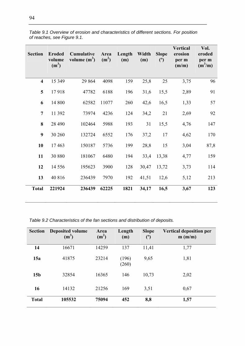
94
Table 9.1 Overview of erosion and characteristics of different sections. For position of reaches, see Figure 9.1.
Section
Eroded volume
(m3)
Cumulative volume (m3)
Area (m2)
Length
(m)
Width
(m)
Slope
(º)
Vertical erosion per m (m/m)
Vol. eroded per m (m3/m)
4 15 349 29 864 4098 159 25,8 25 3,75 96
5 17 918 47782 6188 196 31,6 15,5 2,89 91
6 14 800 62582 11077 260 42,6 16,5 1,33 57
7 11 392 73974 4236 124 34,2 21 2,69 92
8 28 490 102464 5988 193 31 15,5 4,76 147
9 30 260 132724 6552 176 37,2 17 4,62 170
10 17 463 150187 5736 199 28,8 15 3,04 87,8
11 30 880 181067 6480 194 33,4 13,38 4,77 159
12 14 556 195623 3900 128 30,47 13,72 3,73 114
13 40 816 236439 7970 192 41,51 12,6 5,12 213
Total 221924 236439 62225 1821 34,17 16,5 3,67 123
Table 9.2 Characteristics of the fan sections and distribution of deposits.
Section Deposited volume (m3)
Area (m2)
Length (m)
Slope (º)
Vertical deposition per m (m/m)
14 16671 14259 137 11,41 1,77
15a 41875 23214 (196) (260)
9,65 1,81
15b 32854 16365 146 10,73 2,02
16 14132 21256 169 3,51 0,67
Total 105532 75094 452 8,8 1,57

95
The flat area near the moraine ridge has, according to the calculations in Surfer, experienced
net deposition. The slope is around 5º in the area, and the average deposition per meter is 1.3
m, when the area enclosed is 6558 m2. The precipice has not experienced much erosion,
mainly due to limitations in amount of erodible material and the flat area above (resulting in
deposition and lower velocity).
If the total volume eroded (≈ 220 000 m3) over the areas beneath the cliffs are distributed
throughout the 62 200 m2, an average vertical erosion of 3.5 m is obtained, which seems
reasonable when considering field observations.
The first part beneath the precipice, is relatively steep; around 25º, and encloses an area of
4100 m2. The erosion in the area was calculated to be around 15 000 m3. This corresponds to
average vertical erosion per travel distance (m) of almost 4 m. Such deep erosion is also seen
from field investigations where the flow hit the ground beneath the precipice. This is
however not representative for the upper reaches. They are commonly steep, but the erosion
is shallower and the width less than further down the track (see Figure 9.2).
SUPPHELLEDALEN
Figure 9.2 The debris flow track in Tverrdalen seen from the air in the
direction of the flow a few days after the event. The fan is located where
the two valleys meet. Mud is seen to inundate the fields in the flat
lowland. Photo H. Elvehøy.
TVERRDALEN
Fan
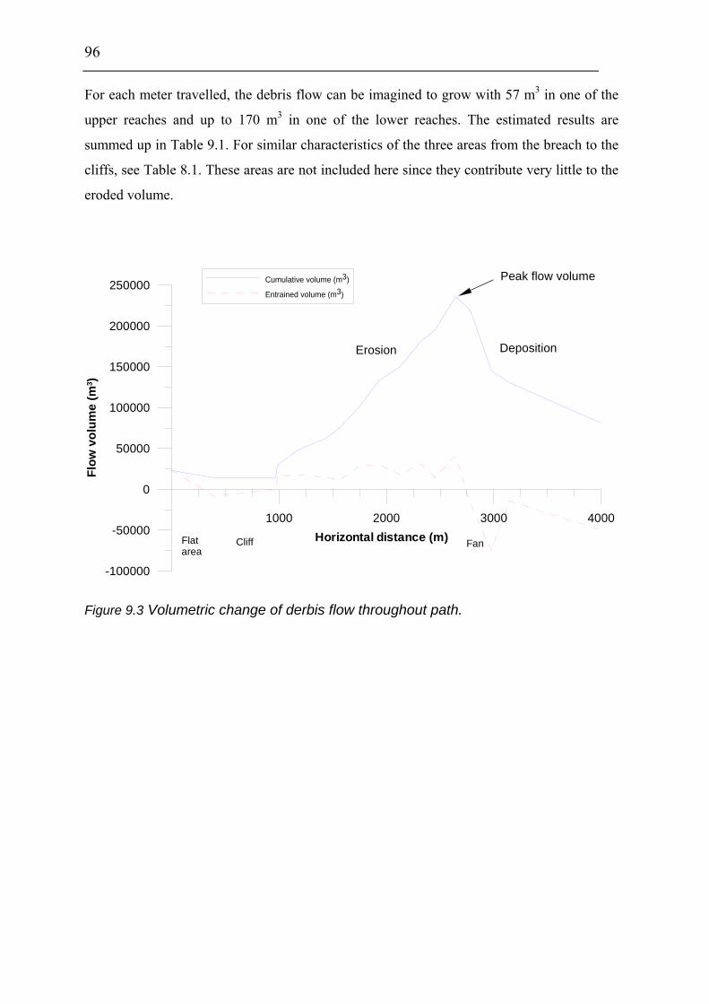
96
For each meter travelled, the debris flow can be imagined to grow with 57 m3 in one of the
upper reaches and up to 170 m3 in one of the lower reaches. The estimated results are
summed up in Table 9.1. For similar characteristics of the three areas from the breach to the
cliffs, see Table 8.1. These areas are not included here since they contribute very little to the
eroded volume.
1000 2000 3000 4000Horizontal distance (m)
-100000
-50000
0
50000
100000
150000
200000
250000
Flow
vol
ume
(m3 )
Cumulative volume (m3)
Entrained volume (m3)
Peak flow volume
Erosion Deposition
FanFlatarea
Cliff
Figure 9.3 Volumetric change of derbis flow throughout path.

97
1000 2000 3000 4000
Horizontal distance (m)
-600
-400
-200
0
200
0
5
10
15
20
25
Slo
pe (o )
SlopeYield rate
Yiel
d ra
te (m
3 /m)
Figure 9.4 Slope and yield rate from below the cliffs to end of deposition area.
-80000
-60000
-40000
-20000
0
20000
40000
0 1000 2000 3000 4000
Horizontal distance (m)
Entr
ainm
ent (
m3)
Figure 9.5 Bar representation of entrainment in every reach, starting from the breach, ending at the end of the mud deposition on the farmland. Red displays entrainment, white represents deposition. Note: the reaches do not have the same length (see Table 9.1 - Table 9.2).
As seen from Table 9.1 and Figure 9.3, the volume grows with a factor of ten from the start
at the moraine breach (0 m) to the beginning of the fan (2644 m). At distance 2644 m from
the breach the volume of the flow is at its peak. Deposited volume does notseem to equal
eroded volume. This may be due both to lack of good deposition data, the loss of sediment to
sea and the differences in density.

98
The volume eroded in the ten reaches studied is around 220 000 m3. When also the around
25 000 m3 from the moraine scar is taken into account, the value grows to almost 250 000
m3. Some material is also eroded from the flat area at around 1000 m.a.s.l. and from the
cliffs. The sides of the eroded gully are probably somewhat steeper than estimated, meaning
that the volume is slightly underestimated. The total eroded volume is suggested to be
approximately 250 000 m3. Some of the material from the upper part is however sedimented
before the precipice, and some deposition occurs at the same time as erosion. This is the
reason for the slightly lower earlier calculated eroded volume (240 000 m3, see Section 8.8).
Eroded volume per travel distance is by several authors called channel debris yield rate, and
is by Huggel et al. (2004) reported to be up to several hundreds of m3/m where lake
outbursts have been the triggering factor. Such high yield rates seem to be linked to
happenings where water is not a limiting factor. This is also considered to be the case in
Fjærland. The yield rates vary from 57 to 212 m3, the largest values typically occurring in
the lower parts of the track. The yield rate of 212 m3/m occurs in an area of average slope
12.6º whilst a higher altitude slope of 25º has a yield rate of only 96 m3/m.
Conclusion These data, supported by field investigations, suggest that flow volume, more than the slope
angle, determines erosion, although they both are important factors. One would expect that
steeper paths produce larger erosion and entrainment (up to a critical slope too steep to
create erosion). It is not expected that the critical slope is as gentle as around 18º. As the
volume of the torrent grows with distance travelled, the potential to erode increases. This is
also dependent on velocity and acceleration, which is believed to increase with distance due
to the entrainment of material and height drop. Entrainment affects the velocity in two ways,
as a slurry of too high sediment concentration will eventually stop in a gentle slope, both due
to viscosity and friction. It is also likely that the debris flow in Fjærland was especially
erosive due the too high content of boulders in the front. The high boulder content increased
with distance due to the higher degree of erosion, the higher yield strength, and the nature of
the bouldery till in the gully. The author considers a flow of moderate to high sediment
concentration to be very erosive. On the other hand, a low sediment flow would produce a
higher velocity, and according to Hungr et al. (2005), debris flows with low sediment
concentration is believed to be more erosive than more sediment rich flows.

99
9.1.2 Deposition
Slope angle seems to be especially important for deposition. Huggel et al. (2004) use an
average slope angle in the determination of debris flow run-out based on empirical data.
Their model is programmed to stop the debris flow when an average angle between initiation
point and end point of 11º is reached. In cases tested this always gave conservative
estimates, which means higher degree of safety for the inhabitants to be protected. In the
case of Fjærland, the average slope angle between the moraine ridge breach and the end of
the fan is around 18º. The mud travelled even further, decreasing the average slope angle.
Hungr et al. (1984) were of the early researchers focusing on entrainment and introducing
the concept of yield rate. They found that deposition starts at between 10 and 14º slope for
unconfined and between 8 and 12º for confined flows. Other researchers have also found
slopes around 10º to result in deposition. However, there is probably no such thing as a
magical slope angle stopping all flows. Topography is also an important factor. The point of
incipient deposition has in all cases studied been found to coincide with the exit of a channel
and an opening of a valley (Hungr et al., 1984). It seemed that the exit from a channel to a
wider area was more important than the slope angle.
This coincides well with the Fjærland case, where main deposition started at 12º, and where
also the valley Tverrdalen, which the debris flow followed, meets Supphelledalen, meaning
that the area available for flow widened.
Conclusion It seems that the boulders deposited within a range of a few degrees (i.e. over a short
terminal distance) whilst finer material may deposit over a large area. Also the exit of a gully
to a wider area is an important factor in deposition. In addition to this, it is likely that flow
volume and velocity would influence the deposition rate and slope. It is generally agreed that
lower sediment concentration (lower yield strength) results in longer run-out and lower
deposition angles. This issue is further treated in Chapter 11.
For a more detailed study of erosion and yield rate, also a velocity profile along the debris
flow path would be interesting for the study of erosion dependence on velocity.

100
10. Debris flows – a literature review
On the basis of field observations and eyewitness reports it can be stated that the Fjærland
flow changed considerably throughout its path. Factors influencing the nature of the flow are
considered to be
• changing water content
• increase in scouring and bulking with time and travel distance,
• change in terrain and vegetation throughout the path
• flow material (concentration, grain size distribution etc.)
• bed material
• deposition of large blocks along the path and in the fan as well as final deposition
of fine material.
Due to this, factors like friction, grain collision, viscosity, density and yield strength may
have had varying importance throughout the event. This chapter presents a discussion of
debris flow mechanics and dynamics based on a literature review and relates earlier findings
to the Fjærland debris flow.
10.1 Flow type related to grain size distribution and maturity
Debris flow material is commonly of variable size. One flow can contain solids of all sizes,
as well as trees and cars. Yet it is common to divide such flows into types according to the
sediment concentration or grain size distribution, because these are parameters influencing
the flow behaviour and the type of force dominating. According to Iverson (1997 a) silt and
clay commonly constitute less than 10 % of the mass. Bulk densities normally range from
1800 to 2300 kg/m3, and volume fraction of grains from 0.5 to 0.8. Experiments have shown
that when the volumetric grain concentration of a mixture is larger than 0.4, the fluid acts
almost like a rigid-plastic solid, but flows like a liquid when pore pressure or agitation is

101
high enough (Iverson & Vallance, 2001). A mixture of 240 000 m3 sediment and 100 000 m3
of water will give a density of 1850 kg/m3 and grain concentration of 0.7.
Solid friction, liquid viscosity and particle collisions play important roles in the mechanics
of a debris flow (Chau et al., 2000). Some dimensionless numbers (like friction number,
Savage number and Bagnolds number) can be useful when dividing debris flows into groups.
It is for example shown that stress due to grain collisions dominate over viscous fluid
stresses if Bagnolds number is above 40 (dispersive stress dominates over viscous stress)
(see below), and that grain collision stresses dominate over grain friction stresses if Savage
number is above 0.1 (Iverson and LaHusen, 1993).
Bagnold number µλρδγ 212&
=B (10.1)
where
γ& = average shear strain rate
δ = typical grain diameter
λ = linear grain concentration
ρ = density of liquid
µ = viscosity
When using a shear strain rate of 2, a grain diameter of 0.1 m, sediment concentration of 0.7
and a viscosity of 300 gives a Bagnold number as low as 5,6*10-5, and a Savage number of
5,7*10-4. This means that viscous stresses should dominate over dispersive and friction
dominates over collision.
Following Coussot (1992) cited in Laigle (1997), debris flows can be divided into two
groups:
• Granular debris flows. Less than 1 % of the solid mass is fine particles smaller than 40 µm.
• Muddy debris flows. Fine-material fraction is higher than 10 % of the solid mass.
Takahashi (1991) uses the terms stony debris flow, immature debris flow, muddy debris flow
and hybrid debris flow. Later he defines different types of debris flows as follows
(Takahashi, 2000):

102
• Stony debris flows: collision of grains dominates the stress. In such a flow the
concentration of large grains is high, the relative depth (depth/size distribution) is
small, and the Bagnold number is large (typically ≥ 20). Particle collisions and
dynamic sieving concentrate the biggest boulders in the front of the flow,
building a head.
• Viscous debris flows: stress due to viscosity dominates. The viscosity of the mass
is very large, and the flow is only turbulent in the front. Both Reynolds and
Bagnold numbers are small.
• Muddy debris flows: stress due to turbulent mixing dominates. Here the particles
are small, but not as small as in a viscous flow, and the motion is very turbulent.
This typically happens when relative depth is large, and Reynolds number is
large. Concentration of large blocks in a head is not common.
• Immature flows: the concentration of coarse particles is under 0.3. Immature
flows are characterised by two separate layers, where the sediment is carried only
by the deepest layer, pure water flowing on top. In contrast, a stony flow is a flow
with only one layer; a collision layer.
• Hybrid flow: develops if the upper layer of water is a turbulent suspension layer.
Figure 10.1
Debris flow regimes and
their dependence on Re,
Ba and H/d. Modified from
Takahashi (2000).
LargeMuddy
Large
Hybrid
Relative depth (H/d)
Reynoldsnumber
Small Viscous Stony
Small
Small LargeBagnold number

103
Armanini et al. (2000) describe some of the same flow regimes in a little bit different way:
They talk about mature slurries, and mean a mass with a liquid content just filling the pores,
while an immature flow has a higher liquid content, with the extra water flowing in a layer
on top, as in Takahashi (2000). They also mention a state of undersaturation, where a basal
shear layer moves a rigid plug. This means that the grains are in the top layer of the flow,
whilst they in an immature flow are at the bottom (see Figure 10.2 ). The authors claim that
the mature condition can occur only in a very limited range of slope angles (θ), the so-called
“θ-mature”. The flow will be undersaturated if the slope is steeper, and immature in a gentler
slope. In addition, transport capacity is an important concept. The authors also connect
concentration to velocity, and state that the lower the concentration the higher the velocity.
This means that a mature debris flow moves relatively slowly, whilst an immature flow
moves fast. When the particles are not in contact (Takahashi, 2000) the mass will flow more
easily. That is; the lower the sediment concentration, the lower the resistance. Particles
settling to the bottom will also enlarge the resistance. Iverson (1997 a) states that the debris
flow solids are made up of grains larger than silt, whereas grains below this limit act as part
of the fluid.
Figure 10.2 Flow figurations depending on water content. Taken from Armanini et
al., 2000.
The eyewitnesses of Fjærland report inconsistently about the layering and order of
ingredients in the torrent. This makes it unclear whether a complete mixture, a layered flow
or separated components approached the fan area. This can be due to the different
geographical positions of the witnesses. As previously explained, the physics of the flow
also changed considerably throughout the event. The flow started out as a water flood and
developed into debris flow after entrainment of bed material. The pictures taken by Eirik

104
Øygard from the cabin Flatbrehytta shows a turbulent flow of high velocity, throwing stones
through the air. This can probably be characterised as a fluidised flow. In such a flow there is
a relative movement between grains and water, meaning that the water is flowing between
the grains, and faster than the grains. The smaller particles move with the speed of the water.
The flow could maybe be characterised as undersaturated (grains on top of moving water) in
the steep slope beneath the cabin, or even hyperconcentrated. The term hyperconcentrated
flow is often used for flows intermediate between floods and debris flows and is more like a
debris flood. Viscosity is the parameter controlling these flows’ rheology the most. A normal
flood has sediment concentration below 4 % (by volume), whilst a debris flow often has
concentration over 60 %. Some authors define the limits of a hyperconcentrated flow as 20-
60 % sediment, others the transition between Newtonian and non-Newtonian fluid as the
lower limit and the yield strength capable to suspend gravel the upper limit (60 Pa) (Pierson,
2005). The latter indicate that the masses shown in Figure 2.4 taken at the precipice can be
characterised as a debris flow, due to the size of the stones seen. It is however not known if
these grains settled rapidly. The upward forces making the particle stay suspended are
turbulence, convection and momentum transfer from grain collisions.
It is unclear whether the flow ended in a mature debris flow. Only a limited range of slope
angles is thought to produce a mature flow. The further down the track the torrent flowed,
the more solids were entrained, resulting in higher sediment concentration. The degree of
erosion, and most importantly the eyewitness observations of a front resembling a wall of
large boulders, proposes that the torrent developed into a mature stony flow.
Most probably only water ran through the valley during the first period of the event. In the
Supphelledalen valley this could only be seen from the upstream side of the fan area as the
river Tverrdøla (which the flow followed) runs on this side. First as the erosional power
increased with growing entrainment (and vice versa), a debris flow front, steep and higher
than the trees, consisting of a mixture of all kinds of sediments, approached the valley. One
witness however reports that the torrent was divided into layers (water on top of granular
material), as described by Armanini et al (2000) as immature debris flow. This type of flow
has a higher liquid content than a mature flow and moves considerably faster. Immature
flows are observed to occur in gentle slopes, which is also a factor indicating that this type
of flow could occur in the depositional area.

105
The same witness tells about stones thrown through the air, indicating a high degree of
collisions in the flow. The blocks found in the path on the track’s flank as well as fractured
stones found up to 25 m from the main track, also points towards grain-grain contact
(collisions).
Turbulence, very high density of the flow, and high pore pressure, fully or nearly liquefying
the mass may also be factors contributing to the transport of large stones, but stones thrown
far out of the main flow indicate grain collisions. This does not support a theory of immature
flow and a layer of water on top, but rather points towards a mature flow. A hybrid flow,
where the upper layer is a turbulent suspension layer, is not a good alternative, as it is not
probable that blocks of the size found on the path can be suspended in a water layer. An
immature flow is also described to have a concentration of coarse particles under 0.3. This is
not probable (see Section 8.6). However, an immature flow may have developed where the
slope is very gentle and deposition has started.
The witnesses on the downstream side of the fan report that the boulders came first and the
water afterwards. This is probably due to the fact that the stony front entrained the forest in
the fan area and deposited, whilst the more liquid fine grained masses flowed further. As the
torrent decreased in size, also the size of the stones entrained decreased, meaning that it later
looked like only water was flowing.
The deposit is also important in determining the type of flow. It is clear that the flood
developed into a debris flow, both due to the size of the boulders, but also due to the inverse
layering described in Section 2.4.
The importance of all this lies in the fact that the stresses and forces change with sediment
concentration and size distribution, and are therefore crucial in any attempt to develop a set
of equations describing the motion of the debris flow. The deposits, as well as witness
statements, are evidence of the high content of coarse, frictional material, meaning that any
equations representing the dynamics must include friction and collision.

106
10.2 The form of a debris flow
Despite the variability in composition and its unsteady and nonuniform behaviour, debris
flows typically approach a steady state condition, with a drop-shaped longitudinal profile,
and constant maximum depth and length (Hungr, 2000; Tognacca, Bezzola and Minor,
2000). This drop is characterized by a steep bouldery front, followed by finer grained,
saturated debris, eventually decaying into a dilute tail (Genevois et.al., 2000, Hungr, 2000;
Iverson, 1997 a; Johnson, 1984; Takahashi, 1991). Coarse debris accumulates at the head of
the debris flow as a result of grain-size segregation and migration within the flow, or
entrainment at the front itself (Iverson, 1997 a; 2003). The high permeability of the coarse
material makes the pore pressure dissipate to near zero at the head. The body behind the
front has a pore pressure close to the weight of the overburden, fully or nearly liquefying the
mass, due to high compressibility and moderate permeability (Iverson, 2003; Iverson et al,
2000). This shows that different forces dominate in different parts of the flow, from a high
resistance front of solid forces to a low resistance tail of fluid forces. The head serves like a
dam, the body pushing on it from behind (Iverson, 2003). This behaviour also results in the
formation of side levees, which retard lateral spreading, concentrate the flow and increase
run-out length (Iverson, 2003). Other explanations of these levees have been proposed by
Johnson (1984), suggesting that dead regions are formed at the sides when the fluid flows in
a channel. Many authors have showed velocity profiles of debris flows, the highest velocity
being in the middle of the flow, decreasing towards the sides. Another explanation can be
waterloss from the mass at lateral margins, making the material on the sides stop earlier than
in the middle.
The motion of debris flows mimics that of wet concrete (Iverson 1997 a), and surges down
its path in waves like water on asphalt. Each surge typically has the coarse front, evincing
the maximum depth of the surge. This behaviour and form of the flow is also observed in
experiments (Genevois et al., 2000), and the interviews with local eyewitnesses in Fjærland
support this theory (see Section 2.1).
A debris flow often starts from rigid masses, transforms during flow to a liquid and ends up
in a rigid deposit (Iverson, 1997 a). This means that both pore fluid pressure and
concentration vary in time and space, and mediate friction and flow resistance (Savage and
Iverson, 2003). Bozhinskiy and Nazarov (2000) describe the process of debris flow in three

107
phases. In the early phase the density of the flow is almost like for water, and the solids
incorporated are not interacting. The next stage occurs soon after initiation. Here density is
very high, and the solids interact in the flow. This stage has longer durability, and eventually
ends in a third stage where the flow decelerates and deposits. The flow density is here close
to limiting, and the water is flowing through a rigid skeleton of grains.
For the Fjærland case, the variations in water and sediment content with time and space is
especially important for the modelling of the flow. The variations are very large, as the flow
has much higher sediment concentration the further down the valley it comes due to ever
increasing entrainment. The flow acted almost like a flood the first 400 m of height drop.
Also time is an important aspect. The sediment first present in the flow was limited (dam
material), and the water flow continued after the removal of this first material. The sediment
concentration at the high flat part before the precipice decreased with time, whilst it
increased at the downstream side of the precipice.
As the debris flow entered the alluvial fan area, it reduced its momentum, spread out and
suddenly stopped. Witnesses describe the settling process as a balloon being punctured. The
shape of a debris flow fan has been shown to resemble the half of an ellipse (Shieh and Tsai,
1997), and this is also recognised in Fjærland. At this point all the kinetic energy has
degraded to irrecoverable forms, and the granular temperature (see Section 10.4) is reduced
to zero (Iverson, 1997 a). Pore pressures in the deposit remain high for a long time after
deposition, but are gradually decreasing with time and consolidation. The maintenance of
pore pressure was also observed in the fine deposits in Fjærland. According to Iverson (1997
b), typical consolidation time (T) varies between 20 minutes and 100 days. The variables are
viscosity (µ), depth of deposit (h), compressibility (C) and hydraulic permeability (k). For a
thicker deposit consolidation time is longer.
kChT µ2
= (Iverson, 1997 b) (10.2 a)
This corresponds to the one-dimensional consolidation relation in soil mechanics:
CvHT
2
∝ (10.2 b)

108
where H is the longest drainage path and Cv is the coefficient of consolidation depending on
permeability, M-modulus and unit weight of water ( wkMCv γ= ) (Lambe and Whitman,
1979).
10.3 Mobilisation
Most mobilisation hypotheses rely on the assumption that debris flows initiate due to
liquefaction, partial or full, caused by elevated pore pressure, and not by shear stress growth.
In addition the increased water content adds weight to the soil. Iverson et al. (1997) describe
three processes mobilising debris flows: Coulomb failure, liquefaction by high pore
pressure, production of granular temperature by grain agitation. A short description of basic
soil mechanics is given in Appendix F.
In the case of Fjærland, erosion is the main mobilisation factor throughout the path. Lin and
Chang (2003) made experiments showing that in debris flows triggered by surface runoff, it
is the erosion of the bed surface that is important in the formation of the flow, not the
increase in pore pressure. According to Tognacca and Bezzola (1997), surface flow is the
most common debris flow trigger in the European Alps. The main processes in the evolution
of such a debris flow are suggested to be:
• water infiltration
• surface runoff
• erosion
• bedload transport
• granular flow of dry material.
Readers are referred to Chen, Lee and Shen (2000), Tarantino and Bosco (2000), Lin and
Chang (2003) and Iverson et al, (1997) among others for a more complete treatment of
mobilisation.

109
10.4 Forces acting in a debris flow
One of the most significant challenges in debris flow modelling is the fact that debris flows
are multiphase flows. The forces acting in the flow are not only due to the different
components, but rather to the interactions between phases and components. The factors
influencing the motion can be summed up to:
• Gravity (body forces)
• Pressure forces
• Viscous stress
• Buoyancy
• Friction grain-bed and grain-grain
• Collisions grain-bed and grain-grain
Ejection Earth pressure
grain-fluid interactions
Collisions viscous sheargrain-grain
friction
gravity grain-bed friction
Figure 10.3 Illustration of forces acting in a debris flow.
Granular temperature is an important phenomenon in soil deformation and motion. It is a
measure of grain agitation (Iverson et al., 1997), and can be defined as the mean square root
of the grain velocity. Higher granular temperature reduces the bulk density and increases the
fluidity of debris (Iverson, 1997 a). It can be generated and maintained by continual
conversion of bulk translational energy to grain fluctuation energy, and can in this way
mobilise a flow from a landslide. Grain agitation can also occur in dry granular materials,
probably being the reason for the rapidness and flowing nature of dry rock fall avalanches

110
like the famous Elm avalanche of 1881. The motion of such sturzstroms (Cruden and
Varnes, 1996) is due to the dispersive stresses created by the momentum exchange between
the colliding particles. No liquid is needed for the material to flow. Such grain agitation is
also a main factor in lifting large boulders and throwing them out of the flow.
10.5 Dynamics and Models
The dynamics of debris flows are less well understood than the initiation and triggering
mechanisms, and different views exist. The most obvious way to study a flow is to treat it as
a fluid and make use of fluid dynamics. Yet, debris exhibit resistance to flow larger than that
of pure water. In addition other forces due to grains may influence the dynamics.
There are several models of momentum transport in debris flows, some relying on rheology,
others on two-phase flow/Coulomb mixture theory. Most models are two dimensional, but
several 3D-models have also been presented. Newton’s second law, conservation of
momentum; (assuming mass is constant) is the basic relation of the models. Here F
is force, m is mass and a is acceleration (dv/dt). The different models vary mostly in the
forces included and how they are represented.
amF ⋅=
10.5.1 Rheological models
Traditional rheological models have long been the most used, like Johnson’s viscoplastic or
Bingham model, Hershel-Bulkley models and later Takahashi’s Bagnold model. Rheological
models combine the relevant relationship between shear stress and shear deformation, with
the Navier Stokes equation. This coupling could in principle permit us to calculate velocity,
pressure and stress etc. of the fluid. A big problem in this approach is to find the correct
rheology. It is most often difficult to measure the parameters needed and the rheological
properties do also change radically both in time and space.

111
The Navier Stokes equation in x-direction:
zyxxPg
zuw
yuv
xuu
tu xzxyxx
x ∂∂
+∂
∂+
∂∂
+∂∂
−−=⎟⎟⎠
⎞⎜⎜⎝
⎛∂∂
+∂∂
+∂∂
+∂∂ τττ
ρρ (10.3)
where
ρ = density, g = gravity,
t = time, P = pressure,
τ = shear stress, u, v, w = velocity in x, y and z direction,
In most rheological models the material is assumed rigid and do not move until a critical
shear stress threshold, the yield strength, is overcome. A Newtonian fluid like water is
different in that it responds immediately and continuously to any stress, and thus has a linear
relationship between shear stress and shear rate. A debris flow is special in that it contains
both fluid and solids, and will not have such a linear relationship. This must be taken into
account in the dynamics. A viscoplastic or Bingham model combines the viscous
deformation and plastic attributes (Iverson, 1997 a) in the representation of τ:
α
ττyuKy ∂∂
+= in general for a Hershel-Bulkley fluid (10.4)
α = 1 Bingham fluid
α > 1 shear thickening fluid
α <1 shear thinning fluid
K = flowing coefficient
τ = shear stress
τy = yield stress
For a Bingham rheology (viscoplastic) this gives:
yu
By ∂∂
+= µττ (10.5)

112
( )sing H yτ ρ= − β for Bingham fluid structure (10.6)
where
H = thickness of flow
y = height to studied point
µB = Bingham viscosity
Basically, the mass does not move until the yield strength, which is treated as static, is
exceeded by the shear stress. This corresponds to the Coulomb strength. To exceed the yield
stress, an equation for the critical thickness Tc of Coulomb debris needed for the mass to
flow is developed by Johnson (1984):
sintan1tan
c
c
Tγ β
ϕβ
⎛ ⎞⎜ ⎟⎝=⎛ ⎞−⎜ ⎟
⎝ ⎠
⎠ (10.7)
where
c = cohesion = τy
γ = unit weight = ρg
β = slope angle
This means that the debris will not flow unless it exceeds the critical thickness (or stops
when the depth becomes less than this). Johnson also had an explanation how debris flows
can transport big boulders. The largest particle (Rm) that a Coulomb debris flow can carry
was found to be:
( )
1−
′=
γγ
ϕγ
bm
fc
R (10.8)
where
γb = unit weight of large particle
f(φ´) = function of friction angle

113
Both friction angle and cohesion must be considered in a model obeying the Coulomb law.
A high φ´ is accompanied with a greater critical thickness than a lower φ´, and failure cannot
occur if friction angle is greater than the slope angle. The fact that debris flows are observed
flowing on very gentle slopes, could mean that the friction angle for debris flows is very low
(Johnson, 1984) or that pore pressure is very high.
Johnson’s model had to be adjusted to include both Coulomb friction and a dynamic
viscosity part. In this model, a central plug of uniform velocity, and a zone of laminar flow
with decreasing velocity to the sides are present. A decrease in slope angle will increase the
thickness of the plug. When the plug thickness equals the thickness of the whole flow, the
flow will stop. This Coulomb-viscous model is written as follows:
⎟⎟⎠
⎞⎜⎜⎝
⎛∂∂
+′+′′=yuc cµϕστ tan (10.9)
where
µc = coefficient of viscosity,
yu∂∂ = shear rate,
So, combining the Bingham model with Coulomb friction gives:
( )cos tany nu uy
τ τ µ σ β∂= + + −
∂ϕ (10.10)
Other theories According to Iverson et al (1997 a), Bingham and also Bagnold theories do not take into
account the pore pressure effects that cause liquefaction nor granular temperature as factors
influencing soil rigidity and motion. Simple rheological models like the Bingham
viscoplastic model can be successfully used for the shear resistance of relatively fine grained
debris flows including a certain fraction of clay (Ayotte and Hungr, 2000, Iverson, 2003).
According to Martino (2003), a Bingham plastic model may overestimate the yield stress
due to shear thinning at low shear rates, and underestimate it when the material is shear
thickening. He concludes that a Hershel-Bulkley model fits a rheological behaviour over a

114
wide range of shear rates. Also Coussot (1992), cited in Laigle (1997), means that the
behaviour of muddy debris flows is well described by a Hershel-Bulkley model. The
rheological parameter K above and yield stress τy are generally expected to increase
exponentially with volumetric concentration (Martino, 2003).
According to Iverson (1997 a, 2003) and Iverson and Vallance (2001), viscoplastic models
do not take into account the interaction between solid grains and viscous fluid. Coarser flows
with a smaller concentration of clay particles behave more like frictional material (Ayotte
and Hungr, 2000) making a Bingham model inappropriate. Moreover, in unliquefied parts of
debris flows, grain to grain contact dominates, and a Coulomb frictional model must be used
(Iverson, 2003). Takahashi’s model uses Bagnold’s findings from 1954 to take the grain
interactions into account in his inertial grain model. Alternative approaches include two-
phase flow models, a Coulomb mixture approach, suggested by Iverson (1997 a). However,
there is more to be done in this field. As mentioned, the rheological models seem to be
appropriate for more viscous and fine grained slurries, but for flows with a higher
concentration of coarser particles (like in Fjærland) and a new model is needed, combining
viscous stress with friction and collision.
Both Iverson (1997 b) and Hungr (2000) have developed 2-D models simulating the surging
behaviour of a debris flow, letting the resistance vary linearly throughout the body of the
flow. Since only a Bingham model is used in this thesis (Chapter 11), the Iverson and the
Hungr models are both briefly presented in Appendix F.
The different types of models proposed seem to have their advantages and disadvantages,
and may be applicable to different types of debris flows. For a further study of what type of
model is representing the flow in Fjærland most accurately, a comparison of a Bingham
rheological model and a model developed by for example Hungr or Iverson would be
valuable.
An attempt to model a flow of the type found in Fjærland meets many complexities. The
mechanical behaviour ranges from bed-load transport possibly to a mature debris flow. The
mechanics alternate both in time and space, thus definition of a common rheology is very
complex. However, only a modified Bingham-model is employed for the work in this master
thesis (Chapter 11).

115
11. Numerical Modelling of the Fjærland debris flow
"Saturated till may flow on the gentlest of slopes" (Hambrey, 1994, p. 114). The statement
shows this soil type’s capability to move, and is commonly seen near glaciers where flow till
can be found. But also further from the glacier saturation makes till unstable. This, in
combination with high erodibility and steep terrain may be reasons for the magnitude of the
dramatic event in Fjærland.
The goals of numerical modelling are:
• To model the run-out
• To study how volume influences erosion and deposition
• To study how slope angle influences erosion and deposition.
• To investigate which type of physics best can illustrate the debris flow in
Fjærland.
Run-out modelling is also useful when considering the design of mitigation structures.
Erosion is an extremely important aspect of the Fjærland case. As the main part of the initial
masses from the moraine ridge was deposited around 1000 m.a.s.l., the whole volume of the
debris flow can be said to be eroded and entrained on the way. A preliminary numerical
model is here suggested.
Different types of physics are tested out in the attempt to model the dynamics of the flow in
Fjærland. Due to the high content of coarse material, a model combining Bingham and
Coulomb friction is being developed by Dr. Fabio De Blasio at the International Center for
Geohazards (ICG), Oslo. The model is based on the BING code and is programmed in
Fortran. The basic form of BING has been modified to include Coulomb friction as well as
sediment entrainment during the debris flow. This 2D-model makes use of the length profile
of the debris flow track in an attempt to simulate the flow.

116
11.1 BING
BING is a simple Lagrangian (reference moves with the flow) dynamical model for the flow
of a Bingham material, developed by Imran et al. in 2001. It is based on two-dimensional
formulations of the Navier Stokes equation and the conservation equation, as only the flow
direction and the direction perpendicular to the bed is taken into account. A length profile
from a terrain model is needed.
The model uses the Hershel Bulkley form (here Bingham) of the yield strength and the
equations are simplified by depth integration. The flow masses are divided into vertical
sections in the flow direction, each node being equally spaced when the model is started. For
each time step, acceleration and position is calculated in every node, resulting in a relative
difference in both acceleration and spacing between the nodes. Equations for both plug layer
and the total mass are developed. The volume per unit width (area) represents the flow
volume in the model. At each node the depth of the flow is calculated.
HA1 y X1 X2
Figure 11.1 Illustration of division of the debris flow into sections in BING.
For a case where both particle-particle and particle-water interactions develop, a model
incorporating the two effects should be used. For this purpose, the BING model is tried
further developed by Fabio De Blasio to include friction and entrainment, better simulating
the Fjærland case.
BING only includes two directions, meaning that the Navier Stokes equation becomes:
1 sinxyxxu u u Pu v gt x y x x y
ττ βρ
∂⎛ ⎞∂∂ ∂ ∂ ∂+ + = − + + +⎜ ⎟∂ ∂ ∂ ∂ ∂ ∂⎝ ⎠
(11.1)
10 cP gy
osβρ∂
= − −∂
(11.2)
When otherwise not noted, all terms are explained in Section 10.5.

117
The continuity equation used can be written as:
0u vx y∂ ∂
+ =∂ ∂
(11.3)
This must be combined with a constitutive relation describing the fluid. For a general
Hershel Bulkey fluid:
( ) ( )1 cosxy yuK g H yy
α
tanτ λ τ λ ρ β ϕ⎡ ⎤∂ ⎡= + + − −⎢ ⎥ ⎣∂⎢ ⎥⎣ ⎦
⎤⎦
1
(11.4)
0 λ≤ ≤ is a measure of importance of cohesion relative to friction. λ of 1 gives the fluid a
cohesive behaviour, whilst a λ of 0 makes it purely frictional. In this way λ is meant to
simulate the degree of contact between grains in the fluid. λ is constant in this model, but
will in nature vary with both x, y and t due to entrainment, building of a bouldery head, the
Brazil nut effect, etc. Assuming a Bingham fluid, α = 1. For the fluid to move,
( ) ( )1 cosy g H y tanτ τ λ λ ρ β ϕ⎡> + − −⎣ ⎤⎦ (11.5)
A further mathematical description of the BING-model is presented in Imran et al (2001).
11.1.1 Erosion
Several simplifications are made in the simulation of erosion/entrainment of sediment. One
of them is the assumption of no-slip condition, meaning that the velocity is zero at the
bottom of the flow. The erosion incorporated is based on shear stress at the base, and does
not take into account the action of grains.
( ) ( )sgn
0
Yxy xy
xy
dh cU U fordt
for
τ τ τ τ
τ τ
= −
= ≤
> (11.6)
where
τ = critical shear rate for erosion, c = erosion constant,
Y = exponent, U = average velocity of the flow,

118
In the model used, Y is set to zero, meaning that erosion does not depend on velocity in the
simulation. This is a simplification. Velocity must however be larger than zero
( ).The erosion is dependent on sine of slope angle and the height of the flow. It is
assumed that erosion starts at elevation 600 m.a.s.l., at the bottom of the cliff.
( )sgn U
The acceleration of each node j is reduced with respect to the case where the debris flow
mass is constant:
ja∗
)( ) (
( )1
1
1 /
1
j
j jj
acceleration without entrainmentaeroded mass original mass of debris flow
dh ta X Xdt A
δ
∗
−
+
=+
⎡ ⎤= + −⎢ ⎥
⎢ ⎥⎣ ⎦
(11.7)
where
a = acceleration without entrainment
Aj = area of each section (Figure 11.1)
Xj = each node (Figure 11.1)
11.2 Challenges
As Chapters 6 and 8 show, especially the water volume involved, but also the sediment
volume, is uncertain.
Solid/water concentration develops from very low (liquid) near the moraine breach to high
as the debris flow approaches the fan area, and does also vary with time. Water continued
flowing also after the initial failure of the moraine ridge, and as the erosion was low in the
high altitude flat area, the solid/water ratio decreased with time in this area. Since the
material from the moraine ridge had very little influence on the masses downstream the
precipice (as most of it deposited in near vicinity of the breach), this decrease in sediment
concentration did not occur in the lower parts of the track before the event was close to
termination.

119
Problems encountered in the modelling process were:
• Water content influences yield strength, density, viscosity and friction angle.
Therefore, these factors should be allowed to vary with the water content. If water
content is being varied, this should also be reflected in yield strength, viscosity,
density and internal friction angle. The relationship between these parameters is not
known. Here the model is run using constant parameters throughout the track.
• The continuous water supply from the glacier. Modelling an abrupt release of a large
volume will not represent reality, as the masses were distributed over time.
• The long duration of the flow.
These problems are not solved. Yet, attempts are made and simplifications taken.
11.3 Running the models
Only one parameter has been changed in each computer run. The importance of each
parameter on run-out is also easier studied in this way. One way to simulate the variations in
water content could be to start out with very low yield strength, increasing with travel
length. This is not done here. The extremes of maximum and minimum yield strength are not
known on beforehand. Therefore different (but constant) yield strengths are tried, and the
effects on run-out and velocity studied.
The parameters used are:
Parameter Y λ φ (º) c (m/sPa) 0τ (kPa) µ (Pa s) γ (g/cm3)
Values used
0
0 0.2 0.5 0.7 1
8
6
6
6
2 10 ,5 10 ,8 10
−
−
−
⋅
⋅
⋅
1
300
1.8

120
11.4 Pure Bingham model – BING 1
The first attempts of modelling the physics of the flow included pure Bingham material,
neglecting friction (BING 1). It is a simple model, but offers a good opportunity for a
parameter study.
11.4.1 Yield strength effects
The simplest case looked at is one with a constant yield strength throughout the track and a
constant volume abruptly released. The existence of a yield stress predicts the presence of a
rigid plug and a critical thickness of the flow, as developed by Johnson (1984). As the
thickness of the debris flow approaches the critical thickness, the velocity gets so low that
the flow stops. Low yield strength is expected to produce long run-outs.
When running a pure Bingham model trying to simulate the viscous slurry of the beginning
of the event, the yield strength was held low. Increasing the yield strength will simulate
debris flows of higher sediment concentration. Low, high and intermediate values were
searched. Three different runs are shown in Figure 11.2, using constant yield strengths of
400, 800 and 10 000 Pa. In all figures where terrain is included, thickness of flow is
exaggerated.
Table 11.1 BING 1. Run-out varying with yield strength in a Bingham model. Volume 20 000m3.
Yield strength (Pa)
Run-out (m)
Elev. at run-out termination
(m.a.s.l.)
Max. velocity (m/s)
Scenario A
400 1541 438 22
Scenario B
800 1060 588 24
Scenario C
10 000 180 986 16
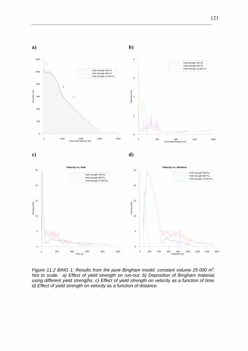
121
a)
0 1000 2000 3000 4000Horizontal distance (m)
0
200
400
600
800
1000
1200
Ele
vatio
n (m
)
Yield strength 400 PaYield strength 800 PaYield strength 10 000 Pa
b)
0 400 800 1200 1600Horizontal distance (m)
0
2
4
6
8
Thic
knes
s (m
)
Yield strength 400 PaYield strength 800 PaYield strength 10 000 Pa
c)
0 200 400 600 800 1000Time (s)
0
5
10
15
20
25
Velo
city
(m/s
)
Yield strength 400 PaYield strength 800 PaYield strength 10 000 Pa
Velocity vs. time
d)
0 200 400 600 800 1000 1200 1400 1600Distance (m)
0
5
10
15
20
25
Vel
ocity
(m/s
)
Yield strength 400 PaYield strength 800 PaYield strength 10 000 Pa
Velocity vs. distance
Figure 11.2 BING 1: Results from the pure Bingham model, constant volume 25 000 m3. Not to scale. a) Effect of yield strength on run-out. b) Deposition of Bingham material, using different yield strengths. c) Effect of yield strength on velocity as a function of time. d) Effect of yield strength on velocity as a function of distance.

122
The slurry of lowest yield strength flows most easily and has the longest run-out. None of
the runs reached the fan, the most mobile ending at elevation approximately 440 m (Figure
11.2 a) and Table 11.1). Due to the low volume included this is not surprising. Only the
initial volume of the moraine ridge scar (25 000 m3) is used (no entrainment).
Most of the material is seen to be deposited on the almost flat plain at elevation around 1000
m.a.s.l. (Figure 11.2 b). This agrees with the field observations. It is also seen that the slurry
of highest yield strength has a thicker deposit than the more easy-flowing mixtures. This also
means that it must terminate first. The yield strength is otherwise not seen to influence for
example form of velocity profile or deposit in any degree. This is seen from Figure 11.2,
where the peaks of oscillations occur at the same position and time.
The highest velocity (25 m/s) occurs in a pronounced peak a few seconds after the initiation
of the flow (Figure 11.2 c and d). The overall trend in the runs is decreasing velocity with
time and distance, possibly due to volume decrease. Effect of volume change is studied later
in this section.
The slurry of lowest yield strength has the overall highest velocity. Higher density due to
the higher content of particles is not taken into account. This could possibly neutralize or
even overrun the yield strength effect.
The masses with the lowest yield strength stopped after 15 minutes.
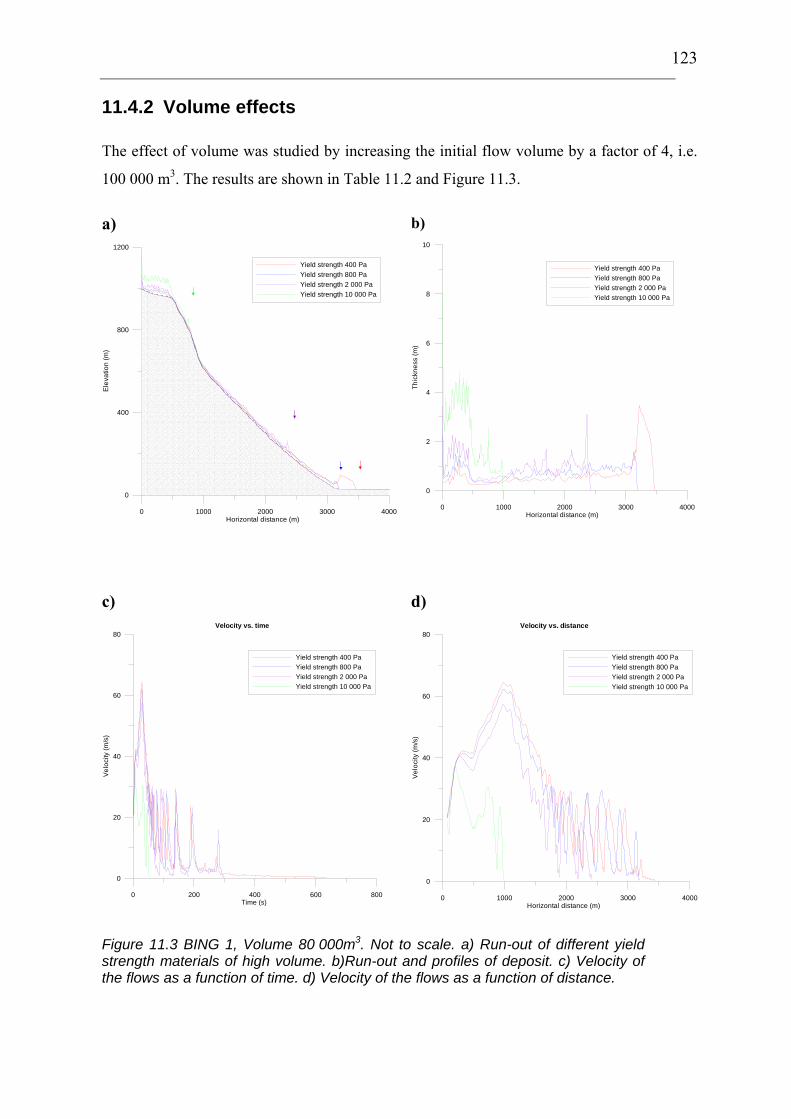
123
11.4.2 Volume effects
The effect of volume was studied by increasing the initial flow volume by a factor of 4, i.e.
100 000 m3. The results are shown in Table 11.2 and Figure 11.3.
a)
0 1000 2000 3000 4000Horizontal distance (m)
0
400
800
1200
Ele
vatio
n (m
)
Yield strength 400 PaYield strength 800 PaYield strength 2 000 PaYield strength 10 000 Pa
b)
0 1000 2000 3000 4000Horizontal distance (m)
0
2
4
6
8
10
Thic
knes
s (m
)
Yield strength 400 PaYield strength 800 PaYield strength 2 000 PaYield strength 10 000 Pa
c)
0 200 400 600 800Time (s)
0
20
40
60
80
Velo
city
(m/s
)
Yield strength 400 PaYield strength 800 PaYield strength 2 000 PaYield strength 10 000 Pa
Velocity vs. time
d)
0 1000 2000 3000 4000Horizontal distance (m)
0
20
40
60
80
Vel
ocity
(m/s
)
Yield strength 400 PaYield strength 800 PaYield strength 2 000 PaYield strength 10 000 Pa
Velocity vs. distance
Figure 11.3 BING 1, Volume 80 000m3. Not to scale. a) Run-out of different yield strength materials of high volume. b)Run-out and profiles of deposit. c) Velocity of the flows as a function of time. d) Velocity of the flows as a function of distance.

124
Table 11.2 BING 1: Run-out varying with yield strength. Volume 100 000m3.
Yield strength (Pa)
Run-out (m)
Elev. at run-out termination
(m.a.s.l.)
Max. velocity (m/s)
Scenario A
400 3460 26 65
Scenario B
800 3190 30 62
Scenario C
2 000 2416 186 57
Scenario D
10 000 986 617 37
Extended run-out was found for all yield strength values. Both masses of 400 Pa and 800 Pa
yield strength reached the valley Supphelledalen and deposited as a thick fan in the area
where the fan is found in the field. Although deposition occurs on the flat high altitude plain,
there are enough masses continuing downwards to reach the fan.
Also the velocity is seen to rise with increasing volume; for all flows passing the precipice a
velocity around 60 m/s was reached here. From this point on the velocity decreases. The
simulated average velocity in Tverrdalen is around 25 m/s, which means 90 km/h, and
decreasing to 20 m/s (72 km/h) when approaching the exit of the gully (fan). The velocity is
computed to grow with increasing volume, as expected, and also with increasing slope.
11.5 Modified Bingham model – BING 2 and 3
11.5.1 Bingham + erosion - BING 2
As discussed, erosion is an important part of the Fjærland event, meaning that this
phenomenon must be accounted for in the numerical model. This is done according to the
explanation and equations in Section 11.1.1.

125
11.5.2 Bingham + erosion + Coulomb friction - BING 3
Due to the high content of granular material, the inclusion of Coulomb friction gives a
physics that is believed to illustrate the flow in a better way than pure Bingham rheology.
The BING model has been extended to include viscous erosion. Erosion due to the grains
and boulders should however also be incorporated in further studies. No-slip condition is
still assumed. Results are shown in and Table 11.4 and Figure 11.4.
First a scenario of Bingham material and erosion was run (BING 2), thereafter Coulomb
friction was added to the model, giving a scenario of a Bingham rheology including
Coulomb friction as well as erosion (BING 3).
Table 11.3 Overview of models used.
BING 1 BING 2 BING 3
Bingham yes yes yes
Erosion/
entrainment
no yes yes
Coulomb friction no no yes
It seems that slope angle has a crucial role in erosion and sedimentation processes, and this
is also reflected in the modelled velocity. Deposition starts when the slope angle becomes
too gentle. In the Fjærland case it seems that a decrease to 12 º is sufficient for deposition to
occur. Volume of flowing mass is suggested to be an even more important factor when it
comes to erosion (see Chapter 9).
Erosion has been included both when running a pure Bingham model (BING 2), as well as in
the Bingham + Coulomb friction model (BING 3). Yield strengths of 400 Pa and 2000 Pa
have been used. The results are seen in Figure 11.4 and Table 11.4. When using 2000 Pa
yield strength in a BING 3 model, the masses stopped before approaching the cliff. The
results of this run are therefore not included in the figures.
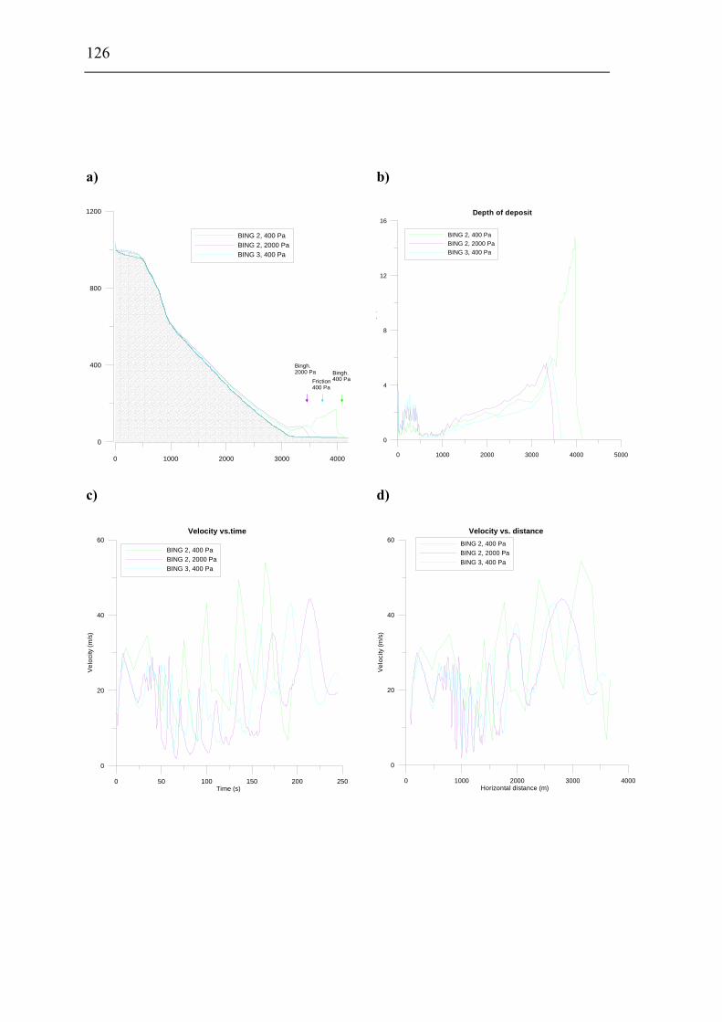
126
a)
0 1000 2000 3000 4000
0
400
800
1200
BING 2, 400 PaBING 2, 2000 PaBING 3, 400 Pa
Bingh.2000 Pa
Friction400 Pa
Bingh.400 Pa
b)
0 1000 2000 3000 4000 5000
0
4
8
12
16
()
BING 2, 400 PaBING 2, 2000 PaBING 3, 400 Pa
Depth of deposit
c)
0 50 100 150 200 250Time (s)
0
20
40
60
Vel
ocity
(m/s
)
BING 2, 400 PaBING 2, 2000 PaBING 3, 400 Pa
Velocity vs.time
d)
0 1000 2000 3000 4000Horizontal distance (m)
0
20
40
60
Vel
ocity
(m/s
)
BING 2, 400 PaBING 2, 2000 PaBING 3, 400 Pa
Velocity vs. distance

127
e)
0 1000 2000 3000 4000
0
2
4
6
8
10
()
BING 2, 400 PaBING 2, 2000 PaBING 3, 400 Pa
Erosion depth
f)
0 50 100 150 200 250Time (s)
0
50000
100000
150000
200000
250000
300000
Volu
me
(m3 )
BING 2, 400PaBING 2, 2000 PaBING 3, 400 Pa
Volume
Figure 11.4 BING 2 and BING 3: Results from running the modified BING-model. Comparison of BING 2 (pure Bingham material with entrainment) and BING 3 (Bingham material with Coulomb friction and entrainment). Not to scale. a) Run-out. b) Run-out and profile of deposit. c) Velocity as a function of time. d) Velocity as a function of distance. e) Erosion depth along debris flow path. f) Accumulated volume.
0 1000 2000 3000 4000Horizontal distance (m)
-4
0
4
8
Ver
tical
ero
sion
(m)
Terrain modelling estimateBingham + erosion1 400 PaBingham + erosion1 2000 PaCoulomb friction + erosion1 400 Pa
Figure 11.5 Erosion depth estimated using terrain model, as well as with the BING model. Terrain model data are shown as black dots. Not to scale.

128
Table 11.4 Run-out and depth of deposit for different types of rheology.
Yield strength (Pa) Run-out (m) Depth of deposit
in fan (m)
Max. velocity
(m/s)
Scenario A
BING 2
400 4100 15 54
Scenario B
BING 2
2000 3349 5,5 44
Scenario C
BING 3
400 3651 6 43
a)
0 1000 2000 3000 4Horizontal distance (m)
0
400
800
1200
Ele
vatio
n (m
)
Debris flow front after 20 seconds
b)
0 1000 2000 3000 400Horizontal distance (m)
0
200
400
600
800
1000
1200
Ele
vatio
n (m
)
Debris flow front after 60 seconds

129
c)
0 1000 2000 3000 4000Horizontal distance (m)
0
200
400
600
800
1000
1200
Ele
vatio
n (m
)
Debris flow front after 120 seconds
d)
0 1000 2000 3000 4000Horizontal distance (m)
0
200
400
600
800
1000
1200
Ele
vatio
n (m
)
Debris flow front after 210 seconds
Figure 11.6 Debris flow front at different time steps. BING 2, yield strength 400 Pa. Not to scale. a)=20 s, b)=60 s, c)=120 s, d)=210 s.
11.5.3 Velocity
The figures show large oscillation in the velocity calculations throughout the track. These
are to be commented in Section 11.7.
Velocities are generally lower when erosion is included than in a pure Bingham model of
large volume (Figure 11.3 c and d and Figure 11.4 c and d). This is expected due to higher
resistance. The velocity seems to increase with distance in BING 2 and 3, as opposed to the
decrease with distance for runs without entrainment. Entrainment results in larger volume,
but also in higher sediment concentration which in turn should slow down the flow.
Velocity is determined by slope angle but also by earth pressure and depth of flow. The
velocity seems to be small just beneath the cliff. This may be due to the fact that the model
predicts little mass to enter this area (small thickness, see Figure 11.4 b). The effect of this
seems to be more important than the increased velocity due to the steep slope. Further down
the track the large volume (thickness of flow) results in high velocities. Only one witness
observation (guestimate) on velocity exists from the field (at the exit of the gully at elevation

130
100 m.a.s.l.), therefore a comparison and discussion of relative importance of these factors
can not be made.
The average simulated velocity in BING 3 is around 15-20 m/s (54-72 km/h), which is
slightly higher than the witness guestimate of 50 km/h. The velocity seems to increase with
distance, and reaches a peak of 43 m/s just before the formation of a fan.
An almost immediate stop of the flow seems to occur in the simulation. This matches well
with the farmers’ descriptions of the event (see Section 2.1.).
11.5.4 Erosion and deposition
As seen from Figure 11.6 b, the modified BING models deposit sediments along the entire
path due to the no-slip condition assumed. The debris flow front is high in the beginning
(flat terrain) and becomes thinner where the terrain steepens. Due to erosion starting at the
bottom of the cliff, the mass gets input of new material so that the flow does not stop due to
thinning. A head can be recognised from the figures as the flow seems to be thickest in the
front. A debris flow has a pulsating nature, but the background for the two peaks seen in C is
unclear and may be due to numerical instabilities.
11.5.5 Depth of deposit
The model uses a width of track of 34 m, meaning that also the deposit area (fan) is 34 m
wide. If spread over a larger area (fan is 75 000 m2), the depth of the deposit and/or the run-
out would decrease. The run-out lengths of the runs described in Figure 11.4 are all slightly
longer than the actual observed run-out (fan). The yield strength used for BING 3 (friction
case) is also very low, resulting in long run-out.
11.5.6 Erosion depth
The erosion depth estimates from BING 3 are close to the dataset presented in Chapter 9.
The model is simple, but overall these estimates using Coulomb friction and entrainment
(blue line, Figure 11.5) matches very well with the observed data and the data estimated
from Surfer (dots, Figure 11.5). The erosion depth is around 3-4 m and decreases towards
zero.
131
However, the distribution of erosion depth throughout the path differs slightly from what is
seen in nature. From the Surfer estimates the depth is almost homogeneous from elevation
600 m.a.s.l., increasing slightly with distance, until an abrupt change towards deposition at
elevation 90 m.a.s.l. (distance 2600 m). Both BING 2 and 3 however predict increase in
erosion depth only for the first 500-1000 m of travel (depending on rheology), followed by
an almost constant decrease towards zero erosion. This may be a result of the simulated
erosion not depending on velocity. The point where no erosion occurs is also predicted at
lower slope and elevation than observed in nature.
The modified BING-models predict erosion depth from the debris flow height and sine of
slope angle. The slope angle is known at all times, flow height must however be calculated.
The flow height is assumed to increase with travel distance and entrainment, which should
give deeper erosion with distance. However, the slope angle decreases (see Figure 9.4). The
combination of the two determines the erosion depth. As previously discussed (Chapter 9),
the deep erosion observed in the end of the debris flow track can be explained by the volume
of flow being of greater importance than the slope angle.
11.5.7 Feedback mechanism
The more erosion is occurring, the larger the volume of the flow gets. As seen above, the
volume influences the velocity of the flow. Higher volume is seen to produce more erosion.
It is also seen that velocity grows with increasing volume, and this is also expected to make
the erosion grow.

132
0 1000 2000 3000 4000 5000Horizontal distance (m)
0
400
800
1200E
leva
tion
(m)
Figure 11.7
A 60 % higher erosion
constant (c = 0.000008
instead of 0.000005) gives
enormous volumes. This run
is stopped after 4 minutes
simulated time but will
continue to flow and entrain.
Not to scale.
An exponential increase in volume is observed in the numerical simulations when the critical
shear rate for erosion approaches zero. This is the proposed reason for the extreme growth of
debris flow mass reported by several authors (e.g. Hungr, McDougall and Bovis, 2005).
( )
sinHgdh dHcdt dt
τ ρ β
τ τ
=
= − = (11.8)
where H = thickness of flow
The behaviour with time:
[0 exp sinsin sin
H H gg gτ τ ]ctρ β
ρ β ρ β⎡ ⎤
= −⎢ ⎥⎣ ⎦
(11.9)
when τ τ> , else H is constant

133
11.6 Summary of results using different models
The results of the numerical modelling show that a pure Bingham flow of constant volume
as small as 25 000 m3 never will reach the fan area, although the yield strength is held very
low. For an initial volume as small as the one found in Fjærland, entrainment is necessary to
achieve long run-outs. A higher initial volume (100 000 m3) would reach the fan area if the
yield strength is held low enough (800 Pa). The velocity of a pure Bingham material,
neglecting entrainment (BING 1), approaches a peak of 60 m/s in the precipice area, and it is
from this point on decreasing due to the combination of loss of material and lowering of
slope.
If including entrainment in the pure Bingham model (BING 2) from beneath the precipice
(starting with an initial volume of 20 000 m3), a flow of 2000 Pa will grow to 250 000 m3
and deposit in the fan area. The velocities are generally lower than if there was no erosion.
Lowest velocities are found at the cliff, increasing to 54 m/s with travel distance due to
increased volume.
When also including Coulomb friction in the erosion model (BING 3), velocities are lowered
even more. The erosion depth is however less than in BING 2. The material of 400 Pa yield
strength (Bingham + friction) seems to act similarly to the BING 2 material of 2000 Pa yield
strength.
This means that increased yield strength decreases run-out length whilst increased volume
generally increases run-out length and velocity. Entrainment is found to be a very important
factor for run-out length.
Decrease in slope generally lowers the velocity of flow. When entrainment is included the
increase in volume however seems more important for velocity than slope angle does. When
it comes to degree of erosion the numerical model predicts that slope angle influences the
erosion more than volume does, and also that an eroding, pure Bingham material of low
yield strength (BING 2) produces deeper erosion than a material including Coulomb friction
(BING 3).

134
11.7 Uncertainties
Values for density and viscosity, as well as yield strength, must be assumed in the model. As
no in situ measurements are done, neither during the debris flow nor during field work, these
parameters contain a high degree of uncertainty. The fact that the parameters may change
considerably during motion should also be taken into account. The grain size distribution is
also not measured, but the soil sediment assumed is till. 1,8 g/cm3 is used for density,
according to the sediment/water distribution found in Section 8.8.
When implementing entrainment in the model, also parameters like yield strength should
vary throughout the track (mostly grow with distance). The model however uses constant
yield strength.
Another problem is the continuous flood of water coming from behind throughout 45
minutes. The aspect of time is not treated any further in the thesis, but the erosion constant
should probably be decreased when considering the long duration of the event.
Modelling deposition is a problem in itself due to the fact that the model is two-dimensional.
This means that 3D effects and topography are not taken into account. Especially deposition
is influenced by this. As discussed in Chapter 9, the exit of a gully is, in addition to slope
and volume, a very important factor for deposition. The spreading of the material can not be
simulated in this model. The computed height of the deposit is therefore also incorrect, since
the deposit can spread only over the 34 m average width.
The velocity is seen to oscillate a great deal. This may have several explanations, for
instance computational instability and the rough topography. The latter means that the sine
of β oscillates, giving also an oscillating velocity. It might give a better picture to make a
smoothing (average) of the topography. Debris flows are known to have a pulsating flowing
behaviour. The oscillations observed in the numerical modelling can most probably not be
related to this phenomenon.
As mentioned, this erosion model does not include velocity.

135
11.8 Velocity estimate based on ballistic stones
Considering that stones have been found 20 m outside the main track (ballistic stones),
obviously thrown through the air, an attempt estimating the velocity of the flow at the point
of “take-off” has been made. Clearly, some assumptions are necessary. The stone is assumed
to be thrown from the flow at an angle of 45 degrees, both upwards and in the direction of
flow (see Figure 11.8 and Figure 11.9). The forest in the area is fairly dense and this
suggests that the stones are likely to have been thrown upwards over the trees to reach a
distance of 20 m.
Figure 11.8 Illustration of angle at which stones are thrown from the main flow.
Figure 11.9 Illustration of how ballistic stones may have been thrown 20 m out of track.
β = 45º
d
x Debris flow
track
45º
Debris flow 20 m

136
Using Newton’s equations for the motion of the stone in the gravity field, the velocity is
found:
0
0
cos
10 20 cos 45 16,8
v g d
v
β= ⋅
= ⋅ = (11.10)
This is the velocity of the ejected stone. If the velocity of the stone is comparable to the
velocity of the debris flow, we find that the velocity at the point (just before entering the fan)
should be 16.8 m/s, or 60 km/h. This fits surprisingly well with the witness guestimate of
velocity (50 km/h).
Most probably the stones have been thrown out of the stream due to inelastic collisions and
fracturing as discussed in Chapter 2. This may implicate that the velocity of the stone may
not have the same velocity as the main flow. This would require a rather different method of
analysis to arrive at an estimate of debris flow velocity, and will not be attempted here.
For derivation of equation 11.10, see Appendix F.

137
12. Mitigation measures
Run-out of a future debris flow in Fjærland of the same size as the 2004-event, will be
affected by the present fan as the terrain has been changed by the deposits. Presently, the
trees are removed in the fan area, which means that a new flow would move easier. The
deposit may lead a new flow further before it starts to deposit, but it could also stop the flow
due to the presence of larger boulders and an open grain structure. Whether the present fan
itself is enough for catching new debris is not known, but it is probable that events of similar
or greater magnitudes will overrun the fan. In that case, mitigation measures should be
taken.
To prevent damage from debris flows, there are in general different countermeasure
alternatives (Schuster, 2000):
• Avoidance – probably the most effective alternative. Avoid developing and house
building in the area at risk.
• Reduction of downstream effects – build retention structures, like check dams
that entrap material, and are designed in such a way that water escapes. Build
deflecting structures to lead the flow in desired direction. Can be combined with
debris basins. A debris basin will trap most of the material (see Figure 12.2).
If an outburst flood from a dam is involved:
• Prevention at dam – many alternatives: Build erosion protection like armouring. Excavation of channel spillway or diversion tunnel. Build check dams on the dam to reduce the velocity of the flow. Install pumps to lower the lake level, as was temporarily chosen in the case of Val Pola until an outlet tunnel was built.
To avoid a rainfall-induced debris flow is not easy, but awareness when building roads and
drainage can reduce the probability of occurence. Vegetation can act in a stabilising way.
Plant roots increase soil strength (Turner, 1996), acting like reinforcement in the soil and
binding unstable soil to more stable layers. However, roots can also act in the opposite
direction (Turner, 1996), to enhance instability. Especially succulent plants absorb great
quantities of water, adding weight to the soil. Roots can also contribute to further weathering
of the soil.

138
The building of a retention and defelcting wall has been started on the downstream side of
the Fjærland fan. This is thought protecting the farm and farmland from flowing water and
fine material. Coarser material will be sedimented in the fan area. If a future event is a fully
grown and high magnitude debris flow running further than the event of 2004, the structure
would most probably fail and the flow pass over.
To catch the high energy coarse masses, a large catchment area would be needed. Another
possibility could be to build sedimentations basins, but these are expensive and material
sedimented need to be removed from time to time. The field observations also point towards
very high energy of the flowing masses.
Figure 12.1 Retention and
deflecting dam being built
between the fan and the farm
Øygard. Photo taken May
2005.
Figure 12.2 Deflecting dam for
a debris flow built in
Hardanger, Norway. Notice
basin and drainage opening.

139
13. Conclusions and recommendations
This thesis highlights the problems related to the physics involved in a debris flow and
attempts to study the factors controlling erosion and entrainment through the recent debris
flow in Fjærland, Western Norway, caused by a natural dam breach. The main goal of the
study has been to provide a thorough documentation of the event, and for this purpose, field
work, interviews with eyewitnesses and terrain modelling have been employed. An attempt
of numerical modelling of the case has been performed in cooperation with Dr. DeBlasio of
ICG, using an extended version of the rheological model BING, including Coulomb friction
and erosion. The results and conclusions of the work are summarised below.
13.1 Conclusions
The study reveals the importance of volume growth through bulking and the development of
grain-to-grain contact in originally very water-rich flows.
Erosion and entrainment of bed material is seen to be very important for run-out length and
velocity of a debris flow. Among the aspects mostly determining erosion, the volume of the
flow has been found to be especially important. In this study a feedback mechanism, poorly
treated in previous literature, is recognised. The phenomenon is also seen in the numerical
modelling and may be part of the reason why debris flows often grow so much and reach
long run-outs. In this case study there is seen little dependence on slope angle (above a
certain value), but this may be due to the fact that the slope angles throughout the main part
of the erosion track only vary between 15 and 20º.
Deposition however, seems to be determined largely by slope angle. In Fjærland deposition
starts at 12º, and all boulders are settled before the slope reaches 4º. Erosion seems not to
appear where the slope is below 12º, but also 3D topography plays a role. Channelisation of
the flow may increase the run-out and reduce the angle of deposition, as well as the exit of a
gully favours spreading and deposition.
Erosion due to the debris flow in Fjærland was extreme; the mass volume growing with a
factor of ten, from around 25 000 m3 to around 240 000 m3 (+/- 10 %) in less than an hour.

140
The large amounts of water involved and the huge bouldery deposit, as well as the finer
sediments inundating the lower farmland, are evidences of the complex dynamics of this
type of mass movement. Large boulders and fractured blocks found 20 m off the main track
point towards a significant grain-to-grain contact and collision impact during the flow.
However, the ratio of the different forces involved varied with time, distance and depth of
the flow.
The BING-model has been modified to include both Coulomb friction and entrainment, but
due to the complexity, numerous simplifications had to be introduced. The model predicts a
run-out, erosion depth and volume very similar to what is seen in field. The results seem
promising, but the velocity estimates may be too high, based on witness accounts. The
velocities are also oscillating, maybe due to instability in the numerical computations. The
problem of varying material properties of the mass throughout the event also needs further
studies.
For mitigation work, an important problem in the use of a model like the modified BING, is
to find the right erosion constant. This will depend on several factors, bed material’s
erodibility being one of them. The application of the model to more case studies would be
fruitful in this process.
The debris flow event in Fjærland seems to be a result of the combination of heavy melting
on the glacier, insufficient opening of drainage channels, and erodible downstream material.
The melting of an ice core in the moraine ridge may also have weakened the dam,
facilitating breaching. There is historical evidence that the normal drainage route for the
glacial lake is through yearly opening of channels towards the icefall in Supphella. When
such channels do not open, a filling of the lake and a breach of the dam is unavoidable.
Earlier floods from the lake through Tverrdalen towards Supphelledalen (drainage route of
the 2004-event) have happened twice during the last 100 years.
The breach in the moraine ridge will be filled by sliding and instability of the breach walls,
making the water level of the lake rise again. Future flooding events will occur, and a
possible global warming could accelerate their frequency. A significant withdrawal of the
glacier could however reveal possibilities for new drainage routes.

141
The potential bulking material along the path will be a limiting factor for the magnitude of
future events. Large amounts of the till material is taken out by the 2004-flow, but the bed is
not depleted. Also the fresh unstable walls of the gully may accelerate erosion if a new flow
occurs.
In a human perspective the magnitude of a new flow will probably be less than the 2004-
event. Historical evidence also points towards the 2004-event being one of the largest that
has occurred at this site. The fan area should however be kept to serve as a catchment area
for a possible flow of new coarse material, whilst finer deposits may be led away from the
farmland by a deflecting dam.
13.2 Personal experience and further work
Problems encountered during the thesis work were several, and mainly related to the terrain
modelling process. A time frame of 5 months has delimited the accuracy of the terrain
models used. This accuracy may be increased by manual effort, and field measurements of
erosion depth at intervals throughout the gully could provide cross-validation of the volume
estimates. Manual field measurements of control points could also make the laser data
applicable to a greater extent. When considering what controls debris flow erosion and
debris flow growth, a study of the effect of velocity and grain size on erosion, is
recommended.
As no adequate model for erosion and entrainment exists, this will be the focus of later work.
Experimental studies are planned in this perspective, to provide insight into the physics of
mass flows and to serve as the basis for numerical modelling. The Fjærland case may be
used to “calibrate” the suitability of the numerical model.
As mentioned, a field investigation of the moraine ridge is planned in June 2005, making use
of geophysical measuring techniques for the purpose to discover whether the ridge is ice
cored. This may be important in the evaluation of the risk of future events, as well as provide
knowledge useful for investigation of similar areas. Dating (for instance C-14) of the
discovered old debris flow deposits in the valleys Tverrdalen and Supphelledalen would also
be important in the estimation of debris flow frequency.

142
13.3 Applicability to other sites
Global warming causes glaciers to melt and accelerates the frequency of storms. Especially
in the Himalayas and Alps, events similar to the Fjærland event will occur. Steep slopes of
many expanding cities worldwide are however very prone to similar debris flows induced by
flash floods. These events are expected to represent an even greater threat.
The case of Fjærland may be applied to a variety of other sites where the release of water in
elevated areas may be a hazard resulting in massive erosion and impact downstream, and the
general findings are applicable to many types of debris flows. This case study will hopefully
provide help in the recognition of similar hazards, as well as in the planning of hazard
zoning and mitigation measures.

143
References
Aarseth, I., Bogen, J., Holtedahl, H., Klakegg, O., Nesje, A., Rye, N., Orheim O., and Roland, E., 1988. Glaciology, hydrology and glacial geology around Jostedalsbreen. A field guide to excursion 10 September – 13 September 1988 organized in conjunction with symposium on snow and glacier research relating to human living conditions. Ed: Olav Orheim. NVE and Norsk Polarinstitutt, Oslo.
Andreassen, L., Elvehøy, H, Kjøllmoen, B., 2004. Glaciological investigations in Norway in 2004. Report no 2 2005, ed: Kjøllmoen, B.. Norwegian Water resources and Energy Diroctorate. p 90.
Armanini, A., Fraccarollo, L., Guarino, L., Martino, R., Bin, Y., 2000. Experimental analysis of the general features of uniform debris flow over a loose bed. In Proceedings of the second international conference on Debris–flow Hazard Mitigation: Mechanics, Prediction, and Assessment, pp. 327-334. Eds. Wieczorek, G.F., Naeser, N.D. Balkema, Rotterdam.
Aschehoug og Gyldendals Store Norske Ettbinds Leksikon, 2004. Eds: Smith-Meyer, T., Reisegg. Ø.. Kunnskapsforlaget, Oslo.
Ayotte, D. and Hungr, O., 2000. Calibration of a runout prediction model for debris-flows and avalanches. In Proceedings of the second international conference on Debris–flow Hazard Mitigation: Mechanics, Prediction, and Assessment, pp. 505-514. Eds. Wieczorek, G.F., Naeser, N.D. Balkema, Rotterdam.
Barstad, B., 2002. Høgdekartlegging med laserskanning frå fly. Institutt for kartfag, NLH. Kartdagane 2002, Oslo.
Barstad, B., 1998. Datafangst for Terreng modellering med Digital fotogrammetri. Fjellanger Widerøe. Foredrag på Forum for fotogrammetri og fjernmåling, 3. og 4. desember 1998.
Bozhinskiy, A.N., Nazarov, A.N., 2000. Two-phase model of debris-flow. In Proceedings of the second international conference on Debris–flow Hazard Mitigation: Mechanics, Prediction, and Assessment, pp. 263-269. Eds. Wieczorek, G.F., Naeser, N.D. Balkema, Rotterdam.
Chau, K.T., Chan, L.C.P., Luk, S.T., Wai, W.H., 2000. Shape of deposition fan and runout distance of debris-flow: Effects of granular and water contents. In Proceedings of the second international conference on Debris–flow Hazard Mitigation: Mechanics, Prediction, and Assessment, pp. 387-395. Eds. Wieczorek, G.F., Naeser, N.D. Balkema, Rotterdam.
Chen, H., Lee, C.F., Shen, J.M., 2000. Mechanisms of rainfall-induced landslides in Hong Kong. In Proceedings of the second international conference on Debris–flow Hazard Mitigation: Mechanics, Prediction, and Assessment, pp. 53-60. Eds. Wieczorek, G.F., Naeser, N.D. Balkema, Rotterdam, 2000.

144
Clague, J.J., Evans, S.G., 2000. A review of catastrophic drainage of moraine-dammed lakes in British Columbia. Quaternary Science Reviews 19 (2000), pp. 1763-1783.
Courivaud, J-R., Lempérière, F., Fry, J-J., 2004. Modelling of Breach formation and Progression. Proceedings from the International Seminar on Stability and Breaching of Embankment Dams, Oslo, Norway, 21-23 October, 2004.
Cruden, D, M., Varnes, D., J., 1996. Landslide types and Processes. In Landslides – Investigation and Mitigation, Special Report 247, Tansportation Research Board, National Research Council. National Academy Press, Washington D.C., pp. 36-75.
Elvehøy, H., NVE, 2005. Pers. comm., 16.02.2005.
Franca, M.J, Braunschweig, F., Almeida, A.B., 2004. RoDaB: dam breaching model with different breach simualtion methodologies. International Seminar on Stability and Breaching of Embankment Dams, Oslo, Norway, 21-23 October, 2004.
Genevois, R., Tecca, P.R., Berti, M., Simoni, A., 2000. Debris-flows in the Dolomites: Experimental data from a monitoring system. In Proceedings of the second international conference on Debris–flow Hazard Mitigation: Mechanics, Prediction, and Assessment, pp. 283-291. Eds. Wieczorek, G.F., Naeser, N.D. Balkema, Rotterdam.
Haldorsen, S., 1983. The characteristics and genesis of Norwegian tills. In Glacial deposits in North-West Europe, pp 11-18. Ed. Ehlers, J., A.A. Balkema, Rotterdam.
Hambrey, M.J., 1994. Glacial environments, pp. 33-80. UCL Press Limited, London.
Hansson, G., Cook, K., 2004. Determination of material rate parameters for headcut migration of compacted earthen materials. Proceedings from the International Seminar on Stability and Breaching of Embankment Dams, Oslo, Norway, 21-23 October, 2004.
Huerta, D.A., Ruiz-Súarez, J.C., 2004. Vibration-Induced Granular Segregation: A Phenomenon Driven by Three Mechanisms. Physical Review letters, vol 92, number 11, pp. 114301-1 – 114301-4.
Huggel, C., Kääb, A., Salzmann, N., 2004. GIS-based modeling of glacial hazards and their interactions using Landsat-TM and IKONOS imagery. Norsk Geografisk tidsskrift – Norwegian Journal of Geography, Vol. 58, pp. 761-73.
Hungr, O., 2000. Analysis of debris flow surges using the theory of uniformly progressive flow. Earth Surface Processes and Landforms, 25 (2000), pp. 483-495.
Hungr, O., McDougall, S., Bovis, M., 2005. Entrainment of material by debris flows. In Debris-flow Hazards and Related Phenomena, pp. 135-158. Eds. Jakob, M. and Hungr, O.. Praxis Publishing Ltd, Chichester, UK.
Hungr, O., Morgan, G.C., Kellerhals, R., 1984. Quantitative analysis of debris torrent hazards for design of remedial measures. Canadian Geotechnical Journal, 21, pp. 663-677.

145
Hyyppä, J., Pyysalo, U., Hyyppä, H., Samberg, A., 2000. Elevation Accuracy of Laser scanning-derived digital terrain and target models in forest environment. Proceedings of EARSeL-SIG-Workshop LIDAR, Dresden/FRG. EARSSeL eProceedings No. 1, pp. 139-147.
Høeg, K., 2004. Lecture in Landslides and mass transport, GEO 4170, UiO, Norway.
Høeg, K., Løvoll, A., Vaskinn, K.A., 2004. Stability and breaching of embankment dams: field test on 6 m high dams. The International journal on Hydropower and Dams, Issue 1, 2004. Aqua –Media International Ltd.
Imran, J, Harff, P., Parker, G., 2001. A numerical model of submarine debris flows with graphical user interface. Computers and Geosciences, 27, pp. 717-729.
Iverson, R.M., 1997 a. The physics of debris flows. Reviews of Geophysics, 35, 3 / August 1997, Paper number 97RG00426. pp. 245-296. (a)
Iverson, R.M., 1997 b. Hydraulic modelling of unsteady debris-flow surges with solid-fluid interactions. In Proceedings of first international conference on Debris–flow Hazard Mitigation: Mechanics, Prediction, and Assessment, pp. 550-560. Ed. Cheng-Iung Chen. American Society of civil Engineers (ASCE), New York. (b)
Iverson, R.M., 2003. The debris-flow rheology myth. In Proceedings of third international conference on Debris–flow Hazard Mitigation: Mechanics, Prediction, and Assessment, pp. 303-314. Ed. Dieter Rickenmann and Cheng-Iung Chen. Millpress, Rotterdam.
Iverson, R.M., Denlinger R.P., LaHusen, R.G, Logan, M., 2000. Two-phase debris-flow across 3-D terrain: Model predictions and experimental tests. In Proceedings of the second international conference on Debris–flow Hazard Mitigation: Mechanics, Prediction, and Assessment, pp. 521-529. Eds. Wieczorek, G.F., Naeser, N.D. Balkema, Rotterdam.
Iverson, R.M., LaHusen, R.G., 1993. Friction in Debris Flows: Inferences from Large-scale Flume Experiments. In Hydraulic engineering, Proceedings of the 1993 ASCE Conference, pp. 1604 – 1609.
Iverson, R.M., Reid, M.E., LaHusen, R.G., 1997. Debris-flow mobilization from landslides. Annu Rev. Earth Planet. Sci., 25. pp. 85-138.
Iverson, R.M., Vallance, J.W., 2001. New views of granular mass flow. Geology; February 2001; v. 29; pp. 115-118.
Jakob, M., Anderson, D., Fuller, T., Hungr, O., Ayotte, D., 2000. An unusually large debris flow at Hummingbird creek, Mara Lake, British Columbia. Canadian Geotechnical Journal, 37, pp. 1109-11025.
Johnson, A.M., 1984. Debris flow, in Slope Stability, Eds: D.Brunsden and D.B. Prios, Wilwy, New York, pp. 257-290.

146
Jørgensen, P., Sørensen, R., Haldorsen, S., 1997. Kvartærgeologi, Landbruksforlaget, Otta, 248 p.
Knight, J.B., Jaeger, H.M., Nagel, S.R., 1993. Vibration-Induced Size Separation in Granular Media: The Convection Connection. Physical Review Letters, vol 70, number 24, pp. 3728 – 3731.
Laigle, D., 1997. A two-dimensional model for the study of debris-flow spreading on a torrent debris fan. In Proceedings of first international conference on Debris–flow Hazard Mitigation: Mechanics, Prediction, and Assessment, pp. 123-132. Ed. Cheng-Iung Chen. American Society of civil Engineers (ASCE), New York.
Some of the original ideas of the above paper found in:
Coussot, P., 1992. Rheologie des laves torrentielles. Thèse de Doctorat de l’Institute National Polytechnique de Grenoble, France, C.E.M.A.G.R.E.F., collection Etude, série Montagne n. 5, 415 p.
Lambe, P.C., 1996. Residual soils. In Landslides – Investigation and Mitigation, Special Report 247, Tansportation Research Board, National Research Council. National Academy Press, Washington D.C., pp. 507-524.
Lambe, T.W and Whitman, R.V., 1979. Soil Mechanics, Wiley Series in Geotechnical Engineering, pp. 406-412. John Wiley and Sons, New York.
Liestøl, O., 1989. Kompendium i Glasiologi. Meddelelser fra Geografisk institutt, Universitetet i Oslo. Naturgeografisk serie. Rapport nr. 15. pp. 79-86.
Liestøl, O., 1995. Kompendium i Glasiologi. Meddelelser fra Geografisk institutt, Universitetet i Oslo. Naturgeografisk serie. Rapport nr. 3. 111 p.
Lin, M.L., Chang, B.S., 2003. Triggering of debris flow caused by groundwater upwelling and surface runoff. In Proceedings of third international conference on Debris–flow Hazard Mitigation: Mechanics, Prediction, and Assessment, pp. 327-338. Ed. Dieter Rickenmann and Cheng-Iung Chen. Millpress, Rotterdam.
Martino, R., 2003. Experimental analysis on the rheological properties of a debris-flow deposit. In Proceedings of third international conference on Debris–flow Hazard Mitigation: Mechanics, Prediction, and Assessment, pp. 363-373. Ed. Dieter Rickenmann and Cheng-Iung Chen. Millpress, Rotterdam.
Meteorological Institute, 2003.
http://met.no/met/klima_2050/forskning/permafrost_norge.html. Visited 15.03.05.
Mueth, D. M., Jaeger, H.M., Nagel, S.R., 1998. Force Distribution in a Granular Medium. Physical Review E57, 3164.
National Geographic, 1998. http://www.nationalgeographic.com/xpeditions/atlas/index.html. Visited 09.05.05.
Nesje, A., 1995. Brelære. Høyskoleforlaget AS, Kristiansand. 118 p.

147
Norsk Bremuseum, 2005. http://www.bre.museum.no. Visited 10.02.05
NVE (Norwegian Water resources and Energy Administration), 2005.
http://www.nve.no/modules/module_109/publisher_view_product.asp?iEntityId=5268. Visited 24.02.2005.
Orheim, O, 1968. Store Supphellebre – En glasiologisk undersøkelse. Hovedoppgave i kvartærgeologi og geomorfologi, UiB.
Paterson, W.S.B., 1994. The Physics of glaciers, pp. 8-25 and pp.103-131. Butterworth-Heinemann, Elsevier Science, Oxford.
Pickert, G., Jirka, G.H., Bieberstein, A., Brauns, J., 2004. Experiments on overtopped homogeneous embankments: Soil/water interaction and breach development. Proceedings from the International Seminar on Stability and Breaching of Embankment Dams, Oslo, Norway, 21-23 October, 2004.
Pierson, T.C., 2005. Hyperconcentrated flow – transitional process between water flow and debris flow. In Debris-flow Hazard and Related Phenomena, pp. 159-202. Eds. Jakob, M. and Hungr, O.. Praxis Publishing Ltd, Chichester, UK.
Remaître, A., Malet, J.-P., Maquaire, O., 2003 a. Study of a debris-flow event by coupling a geomorphological and a rheological investigation, example of the Faucon stream (Alpes-de-Haute-Provence, France). In Proceedings of third international conference on Debris–flow Hazard Mitigation: Mechanics, Prediction, and Assessment, pp. 375-385. Ed. Dieter Rickenmann and Cheng-Iung Chen. Millpress, Rotterdam. (a)
Remaître, A., Malet, J.-P., Maquaire, O., Laigle, D., Ancey, C., Locat, J., 2003 b. Torrential hazard assessment using a debris-flow runout model. The case of the Faucon stream. In Fast slope movements – Prediction and Prevention for risk mitigation, pp. 445-451, ed. Picarelli, L., Patron Editore, Bologna. (b)
Savage, S.B., Iverson, R.M., 2003. Surge dynamics coupled to pore-pressure evolution in debris flows. In Proceedings of third international conference on Debris–flow Hazard Mitigation: Mechanics, Prediction, and Assessment, pp. 503-514. Eds. Dieter Rickenmann and Cheng-Iung Chen. Millpress, Rotterdam.
Schieh, C.-L., Tsai, Y.-F., 1997. Experimental study on the configuration of debris flow fan. In Proceedings of first international conference on Debris–flow Hazard Mitigation: Mechanics, Prediction, and Assessment, pp. 133-142. Ed. Cheng-Iung Chen. American Society of civil Engineers (ASCE), New York.
Scott, K.M., 2000. Precipitation-triggered debris-flow at Casita Volcano, Nicaragua: Implications for mitigation strategies in volcanic and tectonically active steeplands. In Proceedings of the second international conference on Debris–flow Hazard Mitigation: Mechanics, Prediction, and Assessment, pp. 3-13. Eds. Wieczorek, G.F., Naeser, N.D. Balkema, Rotterdam.

148
Schuster, R.L., 2000. Outburst debris-flows from failure of natural dams. In Proceedings of the second international conference on Debris–flow Hazard Mitigation: Mechanics, Prediction, and Assessment, pp. 29-42. Eds. Wieczorek, G.F., Naeser, N.D. Balkema, Rotterdam.
Shinbrot, T., 2004. The brazil nut effect – in reverse. Nature, vol 429, 27 May 2004, pp. 352-353.
Statens Kartverk, 1:50000, Topografisk hovedkartserie M 711, blad 13171.
Takahashi, T., 1991. Debris flow. IAHR Monograph Series. Rotterdam: Balkema. 152 p.
Takahashi, T., 2000. Initiation and flow of various types of debris-flows. In Proceedings of the second international conference on Debris –flow Hazard Mitigation: Mechanics, Prediction, and Assessment, pp. 15-25. Eds. Wieczorek, G.F., Naeser, N.D. Balkema, Rotterdam.
Tarantino, A., Bosco, G., 2000. Role of suction in understanding the triggering mechanisms of flow slides associated with rainfall. In Proceedings of the second international conference on Debris–flow Hazard Mitigation: Mechanics, Prediction, and Assessment, pp. 81-88. Eds. Wieczorek, G.F., Naeser, N.D. Balkema, Rotterdam.
Terzaghi, K., Peck, R.B., Mesri, G., 1996. Soil Mechanics in Engineering Practice, Third Edition. John Wiley & sons, Inc, New York, p. 375.
Tognacca, C., Bezzola, G.R., 1997. Debris-flow initiation by channel-bed failure. In Proceedings of first international conference on Debris–flow Hazard Mitigation: Mechanics, Prediction, and Assessment, pp. 44-53. Ed. Cheng-Iung Chen. American Society of civil Engineers (ASCE), New York.
Tognacca, C., Bezzola, G.R., Minor H.-E., 2000. Threshold criterion for debris-flow initiation due to channel-bed failure. In Proceedings of the second international conference on Debris –flow Hazard Mitigation: Mechanics, Prediction, and Assessment, pp. 89-98. Eds. Wieczorek, G.F., Naeser, N.D. Balkema, Rotterdam.
Turner, K., 1996. Colluvium and Talus. In Landslides – Investigation and Mitigation, Special Report 247, pp. 525-549. Tansportation Research Board, National Research Council. National Academy Press, Washington D.C.
Turton, D., Jonas, D., 2005. Airborne Laser Scanning – Cost effective spatial data. www.gisdevelopment.net/technology(rs/ma03001pf.htm. Visited 10.03.2005.
UNEP, 2005, United Nations Environmental Programme.
http://www.unep.org/Documents.Multilingual/Default.asp?DocumentID=245&Artic eID=3042&l=en
http://www.grida.no/inf/news/news02/news30.htm. Visited 10.05.05.
Watanabe, T., Ives, J.D., Hammond, J.E., 1994. Rapid growth of a glacial lake in Khumbu Himal, Himalaya: Prospects for a catastrophic flood. Mountain Research and Development, Vol. 14, no. 4, pp. 329-340.

149
Østrem, G., Selvig, K. D., Tandberg, K., 1988. Atlas over breer i Sør-Norge. Meddelelse nr 61 fra Hydrologisk avdeling, NVE, p. B-92.

Appendices
Appendices
Appendix A – Witness observations A1 – Interviews with eyewitnesses A2 – Description of debris flow event by Ingebrigt Supphellen A3 – Diary of Eirik Øygard, 1947 debris flow event Appendix B – Terrain profiles B1 – Length profile B2 – Cross profiles Appendix C – Water volume estimates Appendix D – Sediment volume estimates
D1 – Elevation change from 2001 to 2004 D2 – Grid volume computations Appendix E – Gridding reports E1 – Aerial photo 2001 E2 – Aerial photo 2004 E3 – Laser 2004 E4 – Economical map 1:5000 Appendix F – Dynamics of debris flows F1 – Basic mechanics
F2 – Dynamical models F2 – Velocity estimation based on ballistic stone

Appendix A
Appendix A
Witness observations
Used for the reconstruction of the debris flow event in Fjærland, May 8 2004 and the recognition of earlier events.

Appendix A
A1 – Interviews with eyewitnesses
Ingebrigt Supphellen - It started around one o’clock in the afternoon, 8 May 2004. I had been to the petrol station down in Fjærland to tank diesel, and drove directly to my son’s house at Øygardsneset, one of the outermost farms in the valley of Supphelledalen, located 2 km from the fan area. I have a receipt from the petrol station showing that I paid for the diesel at 12:47. The distance between the station and Øygardsneset is a few kilometres, and I guess it would take me around 3 minutes to drive to the farm. The view towards the cabin Flatbrehytta, the valley Tverrdala and the farm Øygard is superb from his son’s house, so Ingebrigt Supphellen saw everything except the break of the moraine. - As I stepped out of the car I heard a roaring sound and felt the ground shake. I turned around - immediately I thought it came from the mountainside at the other side of the river, where it slides are common, especially in winter. As I saw nothing I turned towards the inner part of the valley, where the glacier Supphellebreen often calves. The runup can go over the valley towards the opposite mountainside, causing ground motion and a roaring sound. Then, suddenly, I saw the fountain, black as rock, from the precipice at the cabin Flatbrehytta. His son Ingvar was at the other side of the river, in a tractor with his two children. Ingebrigt tried to signalize and shout. Ingvar heard the sound of the torrent. - At first he thought it was something wrong with his tractor, because he was at the bridge. If he has a load on his tractor he has to drive it in reverse to get over the bridge. With one kid under each arm he ran towards the house to save himself and the children. Well inside the house he called the police. - From the time when I saw the fountain it took a little bit less than half an hour before a huge black front, higher than the tree-tops, speeded down. I thought it took such a long time before I saw anything, so I hoped that nothing was going to reach the valley this time. I would say that the front was between 10-20 meters high, but nearer 10 than 20, steeper than 45º, and had a velocity of around 50 km/h. The slope of the front became gentler as it approached the fan area. The fountain of black water at the precipice was visible for about 2 hours, but with uneven intensity. - The stones came first, the water afterwards. The entire time one could hear the sound of breaking trees through the roar. The river was thick because of the trees, almost as I could walk over it. Luckily, the weather was warm, the snowmelt rapid and the river huge, so that the trees were transported out in the fjord instead of blocking the river. A few days before the event, the glacier had been very active and calved more than usual. The spring was early and sudden. Ingebrigt remembers a smaller slide in 1947, where the river was divided into two parts and two bridges were built. - The road was damaged, but the stones that came down were much smaller than was the case now. Anyway, they were big enough for us to need a stump puller. I helped cleaning the road and fields for stones, and also raising the bridge. This was done so that we did not need to

Appendix A
remove all the stones. So the road had to slope steeply upwards to the bridge. I know for sure that it was the moraine ridge that failed this time also. A now dead relative of mine, Mikkel Supphellen, told me that the river from the glacier Supphellebreen was smaller than normal at this moment. There was also a slide 80 years ago which he has heard about, but do not have any detailed information about. - In the 1700’s though, a huge slide in the same area resulted in the people at the nearest farm Øygard abandoning the area. They left because they feared new slides or because they did not have the equipment to clean up and start farming again. This must be the origin of the name Øygard, as Øygard means abandoned farm. The farm is also called Rødseter in some maps, so that might be the original name.
Ingvar Supphellen, son of Ingebrigt - I was at the other side of the river, in my tractor and with my two kids. I heard the roaring sound when I was at the bridge, and since it is possible that the tractor can overturn, I thought something was happening to the tractor. I jumped out, and as I turned around I saw the fountain from the precipice. Then mud speeded through the forest and splashed between the trees without damaging them. Here are often a lot of tourists in the area, so I ran inside to call the police. As I was on the phone talking to them, through the window I saw the front coming down in the valley. I know the time was 13:02; I got the time from the police. My father came here approximately ten minutes to one, and the slide started immediately after that. The duration of the whole thing was about one and a half hour. As the volume started to reduce, it reduced quite quickly. The front was high and stable until it approached the fan area, and then suddenly collapsed and stopped. The first wave was the biggest; afterwards smaller pulses came, shifting from one side of the fan to the other. I called the police again when the mud passed our house to tell we were ok. Hans Jørgen Øygard was in the forest at the time, in the track of the flow, cutting timber. - He heard the sound and felt the ground shake, through ear guards and helmet! He did not know what or where the sound came from, but he knew he had to run. He found a tractor and drove down to us. Ingvar got a lot of mud on his fields due to the flow. - 10000 m3 I have removed. My fields were inundated by 60 cm (at the cowshed) of mud. There was only mud and no sand on my property. The work was difficult, because it was impossible to walk on the material for several days and it turned liquid as you disturbed it. But as we tested the mass it turned out to be very fertile, so I have used it on my farming land. Now I can say that for me this event has been positive. It is a fact that the farms downstream Tverrdøla and the fan are much more fertile than the farm Supphella further in the valley. That must mean that something is happening here from time to time. He says that during the event of 1947 no stones reached the valley. Ingvar was not born at the time. - At least nothing reached my fields. That means that the event must have been smaller than the 2004-event. There are tales that the farm Øygard was abandoned during the 1700’s due to a big slide. If their fields were hit they probably could not use the land for years.

Appendix A
Per Christian Liseter Liseter lives on the opposite side of the slide, on the upstream side of the fan, and owns parts of the river that was damaged in the event. - I sat outside reading for my exam when the ground started to shake and a roaring sound was heard. My first reaction was to look over the river, to the opposite mountainside, as slides and rock falls are common there. Another possibility was that the glacier was calving. As I turned around I saw a few stones flying through the air, over the house and over the electricity wire further down. I did not know where they came from, so I was a bit afraid. I called my daughters; they were in Fjærland, to tell them to stay until I knew anything more. Then I just ran. I met my neighbour, and we went inside and watched through the window. Suddenly Ivar, my neighbour, shouted out; “we have to run”. A huge black front came surging down. It was visible over the trees! Some stones still came flowing through the air. We ran over to the other side of the fields, looking at it from there. The flow cut down the trees, which were transported with its roots first. Then the stones came, rushing towards Øygard. The water was floating on top of the stony layer, over the trees. This means that some stones came through the air before the black front showed up. The large blocks were not in these first masses, but came afterwards. There was a water layer on top of the stones. - I think a large block settled, and then the pulse changed direction, towards me. After 15 minutes the masses again turned towards Øygard. Totally, it took about one and a half hour. As the flow changed direction towards me and towards Øygard, more and more of the road was chewed up. The only possible connection to other people was at the other side of the river. I tried to calm down, and had fun of the mailbox that was still there, as everything else was damaged. - The wave effect was the scariest thing. All the masses did not come down at once; I guess it was more like 4 or 5 large pulses. They were high above the house, and it seemed that the wave effect influenced the change of direction. - The river ran over my fields inundating them for days after the event. 12,5 crop acres (50 mål = 50 000m2) of good farming land was destroyed. Also the protection structure near the river Storelva, 350 m from the fan was destroyed. During the cleaning up, I digged holes to bury the big blocks, and found fertile soil one and a half meter down, under old slide material like stones and gravel. Also earlier I have found such soil. I have always had a lot of blocks in my fields, and a few years ago I had a man, Kjell Kjøsnes, to dig up the fields with an excavator and clean them. This man found a lot of nice soil deeper down. Tons of good soil was taken up! - We have always been afraid of all the snow avalanches here, and have given up the cowshed. It gets damaged every winter. In earlier times the people here offered to the mountain Vetle Supphellenipa for it to stay stable!

Appendix A
Eirik Øygard
Eirik was at the cabin Flatbrehytta, between the moraine ridge and the precipice. His father built the hut 50 years ago, and Eirik is running it now. He brought food and prepared it for the summer, and had his wife and daughter with him. - I heard a dump sound going up and down. I was standing on the moraine near the precipice, watching the event. After maybe ten minutes, I saw that the muddy water had reached my parabola antenna far down my fields. It was terrible to stand there, just watching my fields being destroyed. I was also afraid my mother was taken by the masses. Luckily, she was not home. At this point he recognised the seriousness of the event and called the alarm central. As the helicopter came to pick them up a few hours later, everything was calm. After the event he has removed 10000 m3 of mud from his fields to be able to use them.
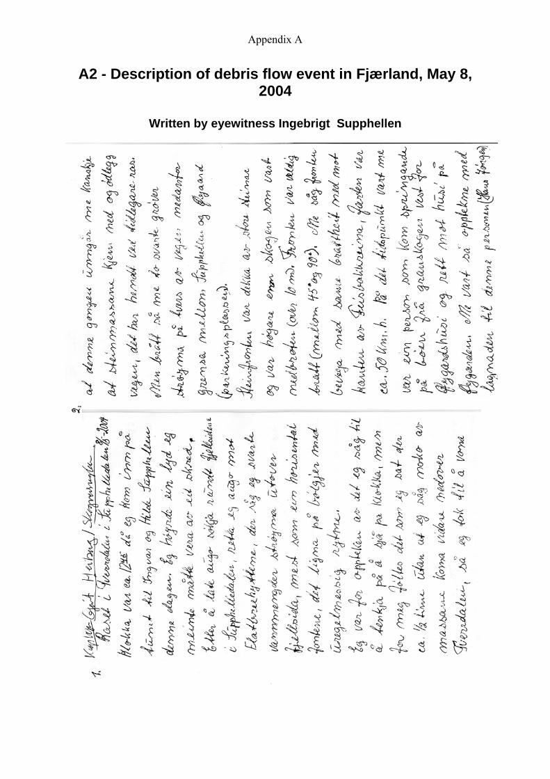
Appendix A
A2 - Description of debris flow event in Fjærland, May 8, 2004
Written by eyewitness Ingebrigt Supphellen

Appendix A Appendix A

Appendix A Appendix A
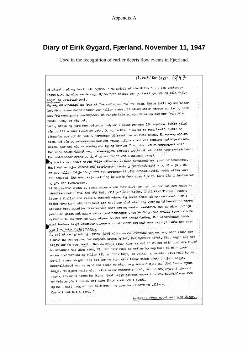
Appendix A
Diary of Eirik Øygard, Fjærland, November 11, 1947
Used in the recognition of earlier debris flow events in Fjærland.

Appendix B
Appendix B
Terrain profiles Generated in Golden Software’s Surfer

Appendix B
B1 - Length profile
050
010
0015
0020
0025
00D
ista
nce
(m)
3000
010
020
030
040
050
060
070
080
090
010
0011
00Elevation (m)
Terr
ain
2001
Figu
re B
1-1
Leng
th p
rofil
e al
ong
debr
is fl
ow tr
ack,
200
1 te
rrai
n.

Appendix B
B2 - Cross profiles
0 10 20 30 40 5Horizontal distance (m)
0
984
988
992
996
1000
1004
Ele
vatio
n (m
)
PROFILE 1: Moraine scar
2001
2004
0 10 20 30Horizontal distance (m)
982984986988990
Ele
vatio
n (m
)
PROFILE 2: Moraine scar
2001
2004
0 10 20 30 40Horizontal distance (m)
972
976
980
984
Ele
vatio
n (m
)
PROFILE 3
2001
2004

Appendix B
0 5 10 15 20 25Horizontal distance (m)
962
964
966
968
970
972E
leva
tion
(m)
PROFILE 4
2001
2004
0 10 20 30 4Horizontal distance (m)
0
956
958
960
962
964
Ele
vatio
n (m
)
PROFILE 5
0 20 40 60Horizontal distance (m)
862864866868870872
Ele
vatio
n (m
)
PROFILE 62001
2004

Appendix B
0 20 40 60 80Horizontal distance (m)
100
800
810
820
830
840E
leva
tion
(m)
PROFILE 7
2001
2004
0 20 40Horizontal distance (m)
610
615
620
625
630
635
640
vat
Ele
ion
(m)
PROFILE 8
2001
2004
0 20 40 60 80Horizontal distance (m)
470
475
480
485
490
495
Elev
atio
n (
PROFILE 9
2001
2004
m)

Appendix B
0 10 20 30 40 5Horizontal distance (m)
0
370
375
380
385
390
395
400
Ele
vatio
n (m
)
PROFILE 10
2001
2004
0 20 40 60Horizontal distance (m)
80
260
270
280
290
300
310
Ele
vatio
n (m
)
PROFILE 11
2004
2001

Appendix B
0 20 40 60 80Horizontal distance (m)
200
210
220
230
240E
leva
tion
(m)
PROFILE 12
2004
2001
0 20 40Horizontal distance (m)
60
135
140
145
150
155
160
165
Ele
vatio
n (m
)
PROFILE 13
2001
2004

Appendix B
0 10 20 30 40 50 60 7Horizontal distance (m)
0
108
112
116
120
124
128E
leva
tion
(m)
PROFILE 14
2001
2004
0 20 40 60 8Horizontal distance (m)
0
96100104108112116
Elev
atio
n (m
)
PROFILE 15
2001
2004
0 20 40 60 80 100 120Horizontal distance (m)
64687276808488
Ele
vatio
n (m
)
PROFILE 16
2001
2004
0 50 100 150 200 250Horizontal distance (m)
3040506070
Ele
vatio
n (m
)
PROFILE 17
20012004

Appendix B
0 20 40 60 80 100 120 140 160Horizontal distnace (m)
10
20
30
40E
leva
tion
(m)
PROFILE 18
0 20 40 60Horizontal distance (m)
970
980
990
1000
1010
Ele
vatio
n (m
)
PROFILE 19
2001
2004
0 20 40 60 80 100Horizontal distance (m)
960
970
980
990
1000
1010
1020
Elev
n (m
)at
io
PROFILE 20
2001
2004
ss sections at intervals throughout debris flow track, showing
pre- and post-flow terrain.Figure B2-1 Illustrations of cro

Appendix C
Appendix C Water volume estimates

Appendix C
Scenarios of different water (and sediment) volumes
Used in the evaluation of water volume possibly involved in the 2004-event. Table C-1 Different water volumes combined ith different sediment volumes in the first and the last cross section of the track.
w
Scenario 1 50 000m3 water Time (s) Area (m2)
Sediment volume (m3)
Velocity (m/s)
Cross section 1 2700 91,5 0 0,2 Cross section 15 2700 Cross section 15 2700 130 450000 1,4
130 250000 0,9
Scenario 2 100 000m3 water Time (s) Area (m2)
Sediment volume (m3)
Velocity (m/s)
Cross section 1 2700 91,5 0 0,4 Cross section 15 2700 130 250000 1,0
ss section 15 2700 130 450000 1,6 CroScenario 3 200 000m3 water Time (s) Area (m2)
Sediment volume (m3)
Velocity (m/s)
Cross section 1 2700 91,5 0 0,8 Cross section 15 2700 130 250000 1,3
ss section 15 2700 130 450000 1,9 CroScenario 4 300 000m3 water Time (s) Area (m2)
Sediment volume (m3)
Velocity (m/s)
Cross section 1 2700 91,5 0 1,2 Cross section 15 2700 130 250000 1,6
ss section 15 2700 130 450000 2,1 CroScenario 5 400 000 m3 water Time (s) Area (m2)
Sediment volume (m3)
Velocity (m/s)
Cross section 1 2700 91,5 0 1,6 Cross section 15 2700 130 250000 1,9
ss section 15 2700 130 450000 2,4 CroScenario 6 500 000 m3 water Time (s) Area (m2)
Sediment volume (m3)
Velocity (m/s)
Cross section 1 2700 91,5 0 2,0 Cross section 15 2700 130 250000 2,1 Cross section 15 2700 130 450000 2,7

Appendix D
Appendix D
dim lum te
Se ent vo e estima s

Appendix D
D1- Elevation change from 2001 to 2004
Showed as col d contours Section 1) Moraine scar:
oure
Legend Figure D-1 Elevation change between aerial photo 2004 and aerial photo 2001. Section 1.
Figure D-2 Elevation change between laser 2004 and aerial photo 2001. Section 1.

Appendix D
Section 2) Flat area
Figure D-4 Elevation change between aaser and aerial photo
Figure D-3 Elevation change between aerial photo 2004 and aerial photo 2001. Section 2
2004 2001. Section 2.
Section 3) Precipice:
igure D-5 Elevation change between aerial hoto 2004 and aerial photo 2001. Section 3.
Figure D-6 Elevation change between laser 2004 and aerial photo 2001. Section 3.
Fp

Appendix D
Section 4) Beneath precipice
Section 4.
Figure D-7 Elevation change between aerial photo 2004 and aerial photo 2001. Section 4.
Figure D-8 Elevation change between laser 2004 and aerial photo 2001.

Appendix D
Section 5) Tunga:
Figure D-9 Elevation change between aerial photo 2004 and aerial photo 2001.
Figure D-10 Elevati
Section 5.
on laser 2004 and aerial photo 2001. Section 5.
Section 6) Tverrdalen:
Figure D-11 elevation change between aerial photo and aerial photo 2001. Section 6.
Figure D-12 Elevation change betwand aerial photo 2001. Section 6.
change between
een laser 2004
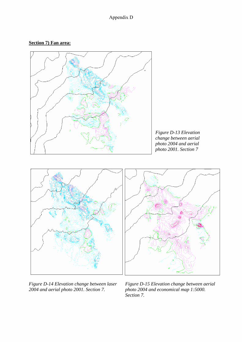
Appendix D
Section 7) Fan area:
etween
2004 and aerial photo 2001. Section 7.
ial
Figure D-13 Elevation change between aerial photo 2004 and aerial photo 2001. Section 7
Figure D-14 Elevation change b laser Figure D-15 Elevation change between aer
photo 2004 and economical map 1:5000. Section 7.

Appendix D
utations
oto generated grid 2001
Minimum: 6814660 Maximum: 6817990
reas
ositive Surface Area [Cut]: 239.92442028364
D2 – Grid volume comp
Generated from Surfer
1) AERIAL PHOTO generated grid 2004 minus aerial ph
Section 1 Moraine scar ———————————————— Grid Volume Computations ———————————————— Wed Mar 02 11:51:54 2005
Upper Surface Grid File Name: C:\geodata\BLN\del5_04-01.grd Grid Size: 1000 rows x 373 columns
X Minimum: 382100 X Maximum: 383340 X Spacing: 3.3333333333333 YYY Spacing: 3.3333333333333
Z Minimum: -13.622536042734 Z Maximum: 1.6938401841255
Lower Surface Level Surface defined by Z = 0
Volumes Z Scale Factor: 1
Total Volumes by: Trapezoidal Rule: -23040.619987584 Simpson's Rule: -23031.377691285 Simpson's 3/8 Rule: -23068.376144571
Cut & Fill Volumes Positive Volume [Cut]: 124.46932230234 Negative Volume [Fill]: 23165.089309887 Net Volume [Cut-Fill]: -23040.619987584
Areas Planar Areas Positive Planar Area [Cut]: 234.60064269777 Negative Planar Area [Fill]: 3659.8438017467 Blanked Planar Area: 4125305.5555556 Total Planar Area: 4129200
Surface APNegative Surface Area [Fill]: 3993.8571091027

Appendix D
Section 2 Flat area
——————————————— Grid Volume Computations ————————————————
ed Mar 02 11:52:32 2005
Upper Surface Grid File Name: Grid Size: 1000 ro
Minimum: 38210
Minimum: 6814660 Maximum: 6817990
33333333333
1
: Rule:
le: 3413581 Rule: 2212506
olumes me [Cut]: 292613 me [Fill]: 122164 ut-Fill]:
r Area [Cut]:
2772.3108276797 4119516.6666667 4129200
Area [Cut]: 60.1934975717 a [Fill]: 2880.7317650429
ipice ———————————————
me Computations —— 005
pper Surface C:\geodata\BLN\del4_04-01.grd
lumns
Minimum: 382100 Maximum: 383340 Spacing: 3.3333333333333
Minimum: 6814660
—
W
C:\geodata\BLN\del7_04-01.grd ws x 373 columns
0 XX Maximum: 383340 X Spacing: 3.3333333333333 YYY Spacing: 3.33 Z Minimum: -5.194645664722 Z Maximum: 5.127811081045 Lower Surface Level Surface defined by Z = 0
olumes VZ Scale Factor:
byTotal Volumes rapezoidal 8526.1852803964 T
Simpson's Ru 8577.988Simpson's 3/8 8536.313
ut & Fill VCPositive Volu 11598.171Negative Volu 3071.9860
[CNet Volume 8526.1852803964 Areas Planar Areas
ositive Plana 6911.0225056536 PNegative Planar Area [Fill]: Blanked Planar Area:
otal Planar Area: T Surface Areas
ositive Surface 71PNegative Surface Are
Section 3 Prec—Grid Volu———————— ——————Wed Mar 02 11:51:32 2 UGrid File Name: Grid Size: 1000 rows x 373 co XXX Y

Appendix D
Y Maximum: 6817990 Spacing: 3.3333333333333
-24.042593456677
1
y:
ule: impson's 3/8 Rule: 24048.63142981
mes me [Cut]:
egative Volume [Fill]: 27121.324809136 Cut-Fill]: 987949
lanar Areas ar Area [Cut]: ar Area [Fill]:
lanked Planar Area: 4101716.6666667 : 4129200
urface Areas rface Area [Cut]: 8644.7631255346
Area [Fill]: 730.02369425
ath prec
Volume Computations ———————————
005
\BLN\del2_04-01.grd 1000 rows x 373 columns
Spacing: 3.3333333333333
Minimum: 6814660 Maximum: 6817990 Spacing: 3.3333333333333
-12.472552189756
Scale Factor: 1
: Rule:
impson's Rule: -48059.53778424 Rule: 2452532
olumes
Y Z Minimum: Z Maximum: 39.735525333542 Lower Surface Level Surface defined by Z = 0 Volumes Z Scale Factor: Total Volumes bTrapezoidal Rule: 22925.611987949 Simpson's R 24628.503310494 S Cut & Fill VoluPositive Volu 50046.936797085 NNet Volume [ 22925.611 Areas PPositive Plan 6164.348188594 Negative Plan 21318.985144739BTotal Planar Area SPositive SuNegative Surface 23 Section 4 Bene ipice ———————————————— Grid—————Wed Mar 02 11:50:42 2 Upper Surface
rid File Name: C:\geodataGGrid Size: X Minimum: 382100
Maximum: 383340 XX YYY Z Minimum: Z Maximum: 2.5213887801567 Lower Surface Level Surface defined by Z = 0 Volumes Z Total Volumes byTrapezoidal -48067.434458661 SSimpson's 3/8 -48128.4 Cut & Fill V

Appendix D
Positive Volume [Cut]: 2863.9418417569 me [Fill]: 300418 ut-Fill]: 4458661
reas r Area [Cut]:
egative Planar Area [Fill]: 22425.715974598 rea: 4102711.1111111
4129200
reas Area [Cut]: 32.4365747033
egative Surface Area [Fill]: 23250.390041129
nga ———
————————————— 11:52:12 2005
6_04-01.grd x 373 columns
Minimum: 6814660 Maximum: 6817990 Spacing: 3.3333333333333
Minimum: -15.046353728695 8861478
otal Volumes by: : -70157.184947588
/8 Rule:
lumes e [Cut]: 555453
lume [Fill]: et Volume [Cut-Fill]: -70157.184947588
s ositive Planar Area [Cut]: 1323.1579033666
nar Area [Fill]: r Area:
otal Planar Area: 4129200
1396.4147000691 egative Surface Area [Fill]: 20305.960905253
rrdalen
Negative Volu 50931.376Net Volume [C -48067.43 APlanar AreasPositive Plana 4063.1729142909 NBlanked Planar ATotal Planar Area: Surface APositive Surface 41N Section 5 Tu——————— ——————Grid Volume Computations ———Wed Mar 02 Upper Surface
a\BLN\delGrid File Name: C:\geodatrid Size: 1000 rowsG
X Minimum: 382100 X Maximum: 383340
Spacing: 3.3333333333333X YYY Z Z Maximum: 3.641667 Lower Surface Level Surface defined by Z = 0 Volumes
1 Z Scale Factor: TTrapezoidal RuleSimpson's Rule: -70049.769291291 Simpson's 3 -69979.053019533 Cut & Fill VoPositive Volum 1291.243Negative Vo 71448.428503041 N Areas Planar AreaPNegative Pla 18654.619874411 Blanked Plana 4109222.2222222 T Surface Areas Positive Surface Area [Cut]: N
Section 6 Tve————————————————

Appendix D
Grid Volume Computations ———————————————— Wed Mar 02 11:51:07 2005
urface : C:\geodata\BLN\del3_04-01.grd
lumns
333333
Minimum: -11.728902103986 Maximum: 2.0653015863519
-103714.19169577 impson's Rule: -103825.99025712
le: -103714.97116161
olumes ositive Volume [Cut]: 465.9367541456
me [Fill]: 2844992 ut-Fill]: 19169577
reas r Area [Cut]: 503135
nar Area [Fill]: lanked Planar Area: 4097450
Area:
urface Areas Area [Cut]: 743.97914601519
32847.787985577
Fan ————————
mputations———
6:46 2005
l1_04-01.grd umns
um: 382100 383340
333333
wer Surface vel Surface defined by Z = 0
1
Upper SGrid File NameGrid Size: 1000 rows x 373 co X Minimum: 382100 X Maximum: 383340
Spacing: 3.3333333X Y Minimum: 6814660 Y Maximum: 6817990
Spacing: 3.3333333333333 Y Z Z Lower Surface Level Surface defined by Z = 0 Volumes Z Scale Factor: 1 Total Volumes by: Trapezoidal Rule: SSimpson's 3/8 Ru Cut & Fill VPNegative Volu 104180.1Net Volume [C -103714. APlanar AreasPositive Plana 719.04018Negative Pla 31030.959814969 BTotal Planar 4129200 SPositive Surface Negative Surface Area [Fill]:
Section 7 ————————
oGrid Volume C Section 7 Fan —————————— ——— Wed Mar 02 11:4 Upper Surface Grid File Name: C:\geodata\BLN\deGrid Size: 1000 rows x 373 col X MinimX Maximum: X Spacing: 3.3333333333333 Y Minimum: 6814660 Y Maximum: 6817990 Y Spacing: 3.3333333 Z Minimum: -13.913928492843 Z Maximum: 6.601791079104 LoLe Volumes Z Scale Factor:

Appendix D
Total Volumes by: Trapezoidal Rule: -156284.03552152
ut & Fill Volumes [Cut]: 28263.651010917 [Fill]:
[Cut-Fill]:
ar Area [Cut]:
egative Planar Area [Fill]: 49433.084129159 ar Area: 666667 rea:
urface Areas ce Area [Cut]: ace Area [Fill]:
generated grid 2004 minus aerial photo generated grid 2001
raine scar ———
—————————————— 14:13:28 2005
\BLN\del5aser-2001.grd
1000 rows x 373
Minimum: 382100 383340 3.3333333333333
3333333
-14.321922278021 -0.10474884524331
ce defined by Z = 0
r:
s by: ule: 8277528 le:
/8 Rule:
mes me [Cut]:
[Fill]: 25777.938277528 -25777.938277528
reas
Planar Areas Positive Planar Area [Cut]: 0 Negative Planar Area [Fill]: 3894.4444444444 Blanked Planar Area: 4125305.5555556 Total Planar Area: 4129200 Surface Areas Positive Surface Area [Cut]: 0 Negative Surface Area [Fill]: 4392.9577909041
Simpson's Rule: -156555.57537525-156504.5820036 Simpson's 3/8 Rule:
CPositive Volume Negative Volume 184547.68653243 Net Volume -156284.03552152 Areas Planar AreasPositive Plan 23050.249204174 NBlanked Plan 4056716.6Total Planar A 4129200 SPositive Surfa 23725.14262855 Negative Surf 51808.479391347 2) LASER Section 1 Mo——————— ——————Grid Volume Computations ——Tue Mar 08 Upper Surface Grid File Name: C:\geodata_lGrid Size: columns XX Maximum: X Spacing: Y Minimum: 6814660 Y Maximum: 6817990 Y Spacing: 3.333333
Minimum: ZZ Maximum:
ace Lower Surfevel SurfaL
Volumes
toZ Scale Fac 1 Total VolumeTrapezoidal R -25777.93
uSimpson's R -25744.127694517 impson's 3 -25880.105985363 S
Cut & Fill Volu
ositive Volu 0 PNegative VolumeNet Volume [Cut-Fill]: A

Appendix D
at area —————
Comput——————————
1 2005
pper Surface Name:
C:\geodata\BLN\del7
columns X Minimum: 382100 X Maximum: 383340 X Spacing: 3.3333333333333 Y Minimum: 6814660 Y Maximum: 6817990 Y Spacing: 3.3333333333333 Z Minimum: -7.1414601919478 Z Maximum: 3.7210042633471
by Z = 0
tal Volumes by: apezoidal Rule: -11334.400463597 mpson's Rule: -11195.647403532 mpson's 3/8 Rule: -11374.296362374
egative Volume [Fill]: 14531.301209807 et Volume [Cut-Fill]: -11334.400463597
reas
3263.7773243266 egative Surface Area [Fill]: 7022.368851044
Section 3 Precipice ———————————————— Grid Volume Computations ————————————————
Upper Surface
rid File Name: C:\geodata\BLN\del4
d ws x 373
3.3333333333333
Spacing: 3.3333333333333
Minimum: -33.490694016405 Maximum: 29.855540278157
ower Surface vel Surface defined by Z = 0
olumes Scale Factor: 1
otal Volumes by: rapezoidal Rule: -62445.723499589 mpson's Rule: -61102.825186629 mpson's 3/8 Rule: -61664.587185912
ut & Fill Volumes ositive Volume [Cut]: 13825.44615675 egative Volume [Fill]: 76271.169656339 et Volume [Cut-Fill]: -62445.723499589
reas lanar Areas ositive Planar Area [Cut]: 1421.5987847168 egative Planar Area [Fill]: 26061.734548616 anked Planar Area: 4101716.6666667
otal Planar Area: 4129200
urface Areas ositive Surface Area [Cut]: 3644.678266211 egative Surface Area [Fill]: 30704.327019055
Section 2 Fl————— ——————Grid Volume ations ——————Tue Mar 08 14:21:5 UGrid File _laser-2001.grd Grid Size: 1000 rows x 373 Lower Surface
d Level Surface define Volumes Z Scale Factor: 1 ToTrSiSi Cut & Fill Volumes
ositive Volume [Cut]: 3196.9007462097 Tue Mar 08 14:06:05 2005 PNN APlanar Areas Positive Planar Area [Cut]: 3077.0180951002 Negative Planar Area [Fill]: 6606.3152382331
66667 Blanked Planar Area: 4119516.66Total Planar Area: 4129200 Surface Areas Positive Surface Area [Cut]: N
G _laser-2001.grGrid Size: 1000 rocolumns X Minimum: 382100 X Maximum: 383340 X Spacing: Y Minimum: 6814660 Y Maximum: 6817990 Y ZZ LLe VZ TTSiSi CPNN APPNBlT SPN

Appendix D
Section 4 Beneath precipice
——————
rid File Name: C:\geodata\BLN\del2
383340 3.3333333333333
14660
3.3333333333333
y Z = 0
by:
[Cut]: 20.222271765041
reas lanar Areas ositive Planar Area [Cut]: 79.08137955823 egative Planar Area [Fill]: 26409.807509331 anked Planar Area: 4102711.1111111 tal Planar Area: 4129200
urface Areas ositive Surface Area [Cut]: 82.083901115784 egative Surface Area [Fill]: 29156.846652193
ection 5 Tunga ——————————————— rid Volume Computations ———————————————
ue Mar 08 14:20:52 2005
pper Surface rid File Name:
C:\geodata\BLN\del6rd
rid Size: 1000 rows x 373 lumns
X Minimum: 382100 X Maximum: 383340
: 3.3333333333333
7571962 1248536
defined by Z = 0
1
otal Volumes by: rapezoidal Rule: -130092.44202445 mpson's Rule: -129689.85824893 mpson's 3/8 Rule: -130268.70853772
0 130092.44202445
et Volume [Cut-Fill]: -130092.44202445
4109222.2222222 4129200
6 Tverrdalen
—————— ——— lume Comput—————— 14:00:46 2005
rid File Name: C:\geodata\BLN\del3
rid Size: 1000 rows x 373
Spacing: 3.3333333333333
um: -13.692993332252 -0.66423129027669
y Z = 0
——————————Grid Volume Computations
—— ——————————————Tue Mar 08 14:00:16 2005 Upper Surface G _laser-2001.grd Grid Size: 1000 rows x 373 columns
382100
X Spacing
X Minimum: X Maximum:
Spacing: X Y Minimum: 68
Maximum: 6817990 YY Spacing: Z Minimum: -14.882675020411 Z Maximum: 0.77247450577914 Lower Surface Level Surface defined b Volumes
Scale Factor: 1 Z Total VolumesTrapezoidal Rule: -118875.20039108 Simpson's Rule: -118945.1591202 Simpson's 3/8 Rule: -118814.19690449
ut & Fill Volumes CPositive VolumeNegative Volume [Fill]: 118895.42266285 Net Volume [Cut-Fill]: -118875.20039108 APPNBlTo SPN S—G—T UG _laser-2001.g
Gco
Y Minimum: 6814660Y Maximum: 6817990Y Spacing: 3.3333333333333 Z Minimum: -16.24978Z Maximum: -0.449641
ower Surface LLevel Surface
olumes VZ Scale Factor: TTSiSi Cut & Fill Volumes Positive Volume [Cut]:
egative Volume [Fill]: NN Areas Planar Areas Positive Planar Area [Cut]: 0 Negative Planar Area [Fill]: 19977.777777778 Blanked Planar Area:
otal Planar Area: T Surface Areas Positive Surface Area [Cut]: 0 Negative Surface Area [Fill]: 22927.896691037 Section ———— ———Grid Vo ations ———— ——————Tue Mar 08 Upper Surface G _laser-2001.grd Gcolumns X Minimum: 382100 X Maximum: 383340 X Y Minimum: 6814660 Y Maximum: 6817990 Y Spacing: 3.3333333333333 Z MinimZ Maximum: Lower Surface Level Surface defined b

Appendix D
Volumes
1
rapezoidal Rule: -176947.70594778 mpson's Rule: -177041.18451503 mpson's 3/8 Rule: -177057.9945283
94778
ositive Planar Area [Cut]: 0 Area [Fill]: 31750 rea: 4097450
as rface Area [Cut]:
egative Surface Area [Fill]: 34596.2399968
7 Fan ——————
——————————— 5
C:\geodata\BLN\del1
lumns
382100
: 6817990
3333333
:
e defined by Z = 0
r:
y: -309974.9644005 -310497.27731788
3/8 Rule: -310279.3445049
]: 4855.6665650563 ll]:
t]: 26.0058594949 ill]:
53.4122533791
Z Scale Factor: Total Volumes by: TSiSi Cut & Fill Volumes Positive Volume [Cut]: 0
94778 Negative Volume [Fill]: 176947.705Net Volume [Cut-Fill]: -176947.705 Areas Planar Areas PNegative Planar Blanked Planar ATotal Planar Area: 4129200 Surface ArePositive Su 0 N Section———— ——————Grid Volume Computations —————Tue Mar 08 13:58:56 200 Upper Surface
rid File Name: G _laser-2001.grd Grid Size: 1000 rows x 373
co X Minimum: X Maximum: 383340 X Spacing: 3.3333333333333 Y Minimum 6814660
Maximum:YY Spacing: 3.333333 Z Minimum: -15.697561087415
Maximum 4.4599154530773 Z Lower Surfac
eLevel Surfac Volumes Z Scale Facto 1 Total Volumes bTrapezoidal Rule:
impson's Rule: SSimpson's
ut & Fill Volumes CPositive Volume [Cut
iNegative Volume [F 314830.63096556 Net Volume [Cut-Fill]: -309974.9644005
reas APlanar Areas Positive Planar Area [Cu 39Negative Planar Area [F 68557.327473838 Blanked Planar Area: 4056716.6666667
otal Planar Area: 4129200 T Surface AreasPositive Surface Area [Cut]: 41Negative Surface Area [Fill]: 72101.919668543

Appendix D
3) AERI 04 – economAL PHOTO 20 ical mection 7 Fan
———— ons Section 7 Fan
———————————— 8:10 2005
king files\d ard.grd umns
Minimum: 382100 383340
333333333333
Maximum: 6817990 ng: 3.3333333333333
6442870751037 58241272
evel Surface defined by Z = 0
otal Volumes by: rapezoidal Rule: 105532.4371339 impson's Rule: 105108.77925305 mpson's 3/8 Rule: 105573.08885247
51581.959497219 Area [Fill]: 20901.373836115
rea: 4056716.6666667 : 4129200
urface Areas ositive Surface Area [Cut]: 54173.099548408
Negative Surface Area [Fill]: 21329.384258307
ap 1:5000
Total Planar Area
S————————————
rid Volume ComputatiG————Mon Mar 14 18:5 Upper Surface Grid File Name: C:\geodata\BLN\Blan el1_2004-oygGrid Size: 1000 rows x 373 col XX Maximum: X Spacing: 3.3 Y Minimum: 6814660 YY Spaci Z Minimum: -4.Z Maximum: 13.6309 Lower Surface L Volumes Z Scale Factor: 1 TTSSi Cut & Fill Volumes Positive Volume [Cut]: 127120.39079521 Negative Volume [Fill]: 21587.953661304
1339 Net Volume [Cut-Fill]: 105532.437 Areas Planar Areas Positive Planar Area [Cut]: Negative PlanarBlanked Planar A
SP

Appendix E
ing reports
G grids from ascii-files
Appendix E
Gridd
eneration of

Appendix E
E1 - Aerial photo 2001
—————————— Mon Feb 28 17:03:34 2005 Elasped time for gridding: 2.39 seconds Data Source Source Data File Name: C:\geodata\flyX Column: A Y Column: B Z Column: C Data Counts Active Data: 143923 Original Data: 166189 Excluded Data: Deleted Duplicates: Retained Duplicates: 22266 Artificial Data: 0 Superseded Data: 0 Univariate Statistics ———————————————————————————————————————————— X Y Z ———————————————————————————————————————————— Minimum: 382099.618 6814659.852 20.074 25%-tile: 382489.618 6815259.851 36.927 Median: 382662.951 6815963.184 281.374 75%-tile: 382856.284 6817203.183 814.774 Maximum: 383339.617 6817993.182 1062.698 Midrange: 382719.6175 6816326.517 541.386 Range: 1239.999 3333.3300000001 1042.624 Interquartile Range: 366.66599999997 1943.3320000004 777.847 Median Abs. Deviation: 180 869.99900000077 252.245 Mean: 382677.65703957 6816190.8518609 408.16416132932 Trim Mean (10%): 382674.48774881 6816176.9704 395.15385561757 Standard Deviation: 246.06614547714 1017.533653465 379.19306606258 Variance: 60548.547949975 1035374.7359339 143787.38134994 Coef. of Variation: 0.92902097241367 Coef. of Skewness: 0.51421480598078
bilder\1.txt
0 22266
Inter-Variable Correlation ———————————————————————————— X Y Z ———————————————————————————— X: 1.000 -0.205 -0.118 Y: 1.000 0.983 Z: 1.000 ———————————————————————————— Inter-Variable Covariance ———————————————————————————————— X Y Z ———————————————————————————————— X: 60548.547949975 -51295.610789026 -10997.512053628 Y: 1035374.7359339 379140.01070575 Z: 143787.38134994 ———————————————————————————————— Planar Regression: Z = AX+BY+C Fitted Parameters ———————————————————————————————————————————— A B C ———————————————————————————————————————————— Parameter Value: 0.13383117338135 0.37188285656179 -2585630.5600308

Appendix E
Standard Error: 0.00071369020343946 0.00017259072244388 1261.0167728621 —————————————————— ————
ter-Parameter Correlations ——————————————
B C ———————————————
-0.408 : 1.000 0.977
1.000 —————
le ——————————————————————————————————————
ource df Sum of Squares Mean Square F —————————————————————————————————————
2 20080724101.859 10040362050.929 2.355E+006 143920 613587184.16882 4263.3906626516 143922 20694311286.028
——————— ————————————————————————
.97034995870662
earest Neighbor Statistics ——————————————————————
—————————————————————————
6349 6349
9842 0317
idrange: 1.6674999996321 34.6205 991
54808E-010
ean: 3.3182765700475 1.0260278690689
42
oef. of Variation: 0.066603046772074 1.5061586402879 4.943174132778 6.552595821589
oot Mean Square: 3.3256283068076 1.8549590306467 ean Square: 11.05980363504 3.4408730053779
————————————————————
4
——————————————————————————— Z ID Status
——————————————————————————————————— Retained Deleted
ined 6816416.5
——————————————————————
In—————————————— A —————————————A: 1.000 -0.205 BC: ———————————— ——————————— ANOVA Tab——————S———————Regression: Residual: Total: —————————— ——— Coefficient of Multiple Determination (R^2): 0 N——————————— Separation |Delta Z| ————————Minimum: 0.0009999992325902 0 25%-tile: 3.332999999 0.212 Median: 3.332999999 0.702 75%-tile: 3.332999999 1.475 Maximum: 3.334000000 69.241 MRange: 3.3330000007 69.241 Interquartile Range: 3.4924596 1.263 Median Abs. Deviation: 0 0.564 MTrim Mean (10%): 3.3329999997272 0.88371592900541Standard Deviation: 0.22100732959755 1.54536074017Variance: 0.04884423973584 2.3881398172719 CCoef. of Skewness: -1 1 RM————————————— Complete Spatial Randomness Lambda: 0.034820143546037
7 Clark and Evans: 1.238391192999 Skellam: 348247.5300017
Exclusion Filtering
xclusion Filter String: Not In Use E
uplicate Filtering DDuplicate Points to Keep: First X Duplicate Tolerance: 0.00014 Y Duplicate Tolerance: 0.00039
ates: Deleted Duplic 22266 Retained Duplicates: 22266 Artificial Data: 0 —————————————————
Y X—————————382186.28 6816419.8 383.576 83436
6816419.8 382.992 108817 382186.28
6816416.5 303 6 382189.62 382. 8335 Reta382189.62 382.168 108756 Deleted

Appendix E
382189.62 6816419.8 383.074 83437 Retained
82189.62 6816419.8 383.432 108818 Deleted
83517 Retained Deleted
6816426.5 385.509 83597 Retained 6816426.5 387.097 108954 Deleted
83357 Retained 82192.95 6816416.5 382.957 108757 Deleted
Retained 5 6419.8 eted
.2 Deleted
Retained 82192.95 6816426.5 389.203 108955 Deleted
82192.95 6816429.8 388.335 83677 Retained 29.8 391.659 109029 Deleted
6816433.2 390.387 83757 Retained 109107 Deleted
6816413.2 .166 83277 Retained 6816413.2 .473 108700 Deleted
6816416.5 .163 83358 Retained 82196.28 6816416.5 384.193 108758 Deleted
6816419.8 .62 83439 Retained 816419.8 108820 Deleted
82196.28 6816423.2 387.019 83519 Retained 6816423.2 .659 886 Deleted
816426.5 743 99 Retained 6816426.5 492 956 Deleted
6816429.8 93 78 Retained 015 030 Deleted
.8 58 Retained 6816433.2 7.153 108 Deleted
82196.28 6816436.5 395.203 83837 Retained 399.377 109190 Deleted
6816439.8 82 83916 Retained 816439.8 .563 109276 Deleted
82199.62 6816413.2 384.306 83278 Retained 6816413.2 384.209 108701 Deleted
82199.62 6816416.5 386.278 83359 Retained 6816416.5 386.17 108759 Deleted
6816419.8 388.432 83440 Retained 6816419.8 388.093 108821 Deleted
6816423.2 390.268 83520 Retained 6816423.2 391.012 108887 Deleted
82199.62 6816426.5 392.264 83600 Retained Deleted
Retained
82199.62 6816433.2 396.454 83759 Retained
3 382189.62 6816423.2 384.43 382189.62 6816423.2 384.857 108884 382189.62 382189.62 382192.95 6816416.5 382.868 3 382192.95 6816419.8 384.182 83438 382192.9 681 384.997 108819 Del 382192.95 6816423.2 385.106 83518 Retained 382192.95 6816423 386.78 108885 382192.95 6816426.5 386.672 83598 3 3382192.95 68164 382192.95 382192.95 6816433.2 394.41 382196.28 382 382196.28 382 382196.28 384 3 382196.28 385382196.28 6 386.351 3382196.28 388 108 382196.28 6 388. 835382196.28 391. 108 382196.28 390.6 836382196.28 6816429.8 394. 109 382196.28 6816433.2 392 837382196.28 39 109 3382196.28 6816436.5 382196.28 397.6382196.28 6 401 3382199.62 3382199.62 382199.62 382199.62 382199.62 382199.62 3382199.62 6816426.5 393.503 108957 382199.62 6816429.8 394.312 83679 382199.62 6816429.8 396.416 109031 Deleted 3382199.62 6816433.2 399.287 109109 Deleted

Appendix E
382199.62 6816436.5 398.816 83838 Retained
82199.62 6816439.8 401.35 83917 Retained
82199.62 6816443.2 403.922 83995 Retained
82202.95 6816409.8 386.502 83197 Retained
82202.95 6816413.2 388.083 83279 Retained
82202.95 6816416.5 389.661 83360 Retained
82202.95 6816419.8 391.837 83441 Retained
82202.95 6816423.2 394.174 83521 Retained
82202.95 6816426.5 396.313 83601 Retained
82202.95 6816429.8 398.367 83680 Retained
82202.95 6816433.2 400.274 83760 Retained
82202.95 6816436.5 402.42 83839 Retained
82202.95 6816439.8 404.598 83918 Retained
82202.95 6816443.2 406.787 83996 Retained
82202.95 6816446.5 408.759 84073 Retained
82202.95 6816449.8 410.245 84150 Retained
82206.28 6816409.8 389.371 83198 Retained
82206.28 6816413.2 391.047 83280 Retained
82206.28 6816416.5 392.557 83361 Retained
82206.28 6816419.8 394.888 83442 Retained
82206.28 6816423.2 397.165 83522 Retained
82206.28 6816426.5 399.254 83602 Retained
82206.28 6816429.8 401.307 83681 Retained
ore ... ———— —————— ——————— ——
reakline Filtering
ing: t In Use
382199.62 6816436.5 401.897 109191 Deleted 3382199.62 6816439.8 404.193 109277 Deleted 3382199.62 6816443.2 406.229 109367 Deleted 3382202.95 6816409.8 384.656 108648 Deleted 3382202.95 6816413.2 386.581 108702 Deleted 3382202.95 6816416.5 388.746 108760 Deleted 3382202.95 6816419.8 391.065 108822 Deleted 3382202.95 6816423.2 393.45 108888 Deleted 3382202.95 6816426.5 396.21 108958 Deleted 3382202.95 6816429.8 398.953 109032 Deleted 3382202.95 6816433.2 401.464 109110 Deleted 3382202.95 6816436.5 404.199 109192 Deleted 3382202.95 6816439.8 406.27 109278 Deleted 3382202.95 6816443.2 408.223 109368 Deleted 3382202.95 6816446.5 409.644 109462 Deleted 3382202.95 6816449.8 410.483 109560 Deleted 3382206.28 6816409.8 387.68 108649 Deleted 3382206.28 6816413.2 389.867 108703 Deleted 3382206.28 6816416.5 391.948 108761 Deleted 3382206.28 6816419.8 394.365 108823 Deleted 3382206.28 6816423.2 396.635 108889 Deleted 3382206.28 6816426.5 399.239 108959 Deleted 3382206.28 6816429.8 401.423 109033 Deleted M——————— ——————— —————— ————— B Breakline Filter No

Appendix E
Gridding Rules angulation wi olation
nisotropy Ratio: 1 le:
utput Grid : \geodata\flybi
00 rows x 37otal Nodes: 373000
8962 : 4038
2100
Maximum: 383340 3333333333
Minimum: 6814660 17990 3333333333
.1598192947
25%-tile: 136.33052515263 2.7561157823.988484913
Maximum: 1062.1982769148
1.179048104 Range: 1042.0384576201
ange: 7.657959761Deviation 6.332626894
4.5708623350%): 3.862724051
Standard Deviation: 316.96838323507 0468.955970
Coef. of Variation: 0.74656179063188 ness: 3919348815
Root Mean Square: 529.83900678856 : 0729.373114
Gridding Method: Tri th Linear InterpAAnisotropy Ang 0 OGrid File Name C: lder\1.grd Grid Size: 10 3 columns TFilled Nodes: 25Blanked Nodes 11 Grid GeometryX Minimum: 38XX Spacing: 3.3 33 YY Maximum: 68Y Spacing: 3.3 33 Grid StatisticsZ Minimum: 20 14 ZZ Median: 38 15 Z 75%-tile: 65 81 Z Z Midrange: 54 74 ZZ Interquartile R 51 17 Z Median Abs. : 25 78 Z Mean: 42 18 Z Trim Mean (1 41 26 ZZ Variance: 10 65 ZZ Coef. of Skew 0.4 575 ZZ Mean Square 28 69

Appendix E
E2 - Aerial photo 2004 ———— 4 2005
for gridding: 4.28 seconds
ta: cates: icates:
Data:
stics ——————————— ————————————————
Y Z ——————————— ———————————————— 6814666.519 20.112 6815656.518 207.614
6816383.184 443.073 6817383.183 890.944
6818283.182 1146.747 6816474.8505 583.4295 3616.6629999997 1126.635
ile Range: 1726.665 683.33 n: 846.66500000004 331.133
6816490.2583985 521.22701777388 0%): 6816489.5710823 517.59350503006
957.94572876683 357.72964068445 917660.01926261 127970.49582423
0.68632213696882 0.19140447185483
————————— ————————————————
ter-Variable Correlation ———————————————————————————
X Y Z ———————————————————————————
: 1.000 0.378 0.364 : 1.000 0.984 : 1.000 ———————————————————————————
ter-Variable Covariance ———————————————————————————————
X Y Z ———————————————————————————————
: 109631.73693826 119853.37232484 43093.260209648 : 917660.01926261 337103.63041912 : 127970.49582423 ———————————————————————————————
lanar Regression: Z = AX+BY+C
itted Parameters ———————————————————————————————————————————
A B C ———————————————————————————————————————————
arameter Value: -0.010044077519262 0.36814010955958 -2505058.8839297 tandard Error: 0.00042405971936356 0.00014659053156965 949.86564255272 ———————————————————————————————————————————
——————Mon Feb 28 17:07:2Elasped time
e Data Sourcata\flybilder\4.txt Source Data File Name: C:\geod
X Column: A Y Column: B
Column: C Z
Data CountsActive Data: 254137
a:Original Dat 319464 xcluded Da 0 E
Deleted Dupli 65327 Retained Dupl 65327
ta:Artificial Da 0 uperseded 0 S
tatiUnivariate S
—————— ——————————— X
—————— ———————————Minimum: 381866.285
5%-tile: 382422.951 2Median: 382649.617
75%-tile: 382872.95 Maximum: 383586.283 Midrange: 382726.284
ange: 1719.998 RInterquart 449.99900000001 Median Abs. Deviatio 223.33300000004
Mean: 382649.3014295 rim Mean (1 382647.39870378 T
Standard Deviation: 331.10683613942 Variance: 109631.73693826 Coef. of Variation:
s: Coef. of Skewnes ——————— ————————————
In— —XYZ— In— —XYZ— P F— —PS—

Appendix E
Inter-Parameter Correlations ——————————————————
B ————————————
0.227 0.987
1.000 —————
le ——————————————————————————————————————
df Sum of Squares Mean Square F —————————————————————————————————————
2 31428795776.588 15714397888.294 3.653E+006 254134 1093242120.6954 4301.8333662375 254136 32522037897.284
——————— ————————————————————————
0.96638457515644
Statistics ——————————————————————
6349 0006 9842
0317
6321 7991
010
5
.046216675816748 .3102071522002 1.584475020201 2.952341911195
11.08520026372 3.5403881207341 ————
: 2
Not In Use
0
——————————————————————————————————— Status
Retained ted
ained Deleted
82086.28 6816166.5 381.487 96123 Retained 82086.28 6816166.5 381.505 164119 Deleted
—————————— C A
————————————————A: 1.000 0.378
: 1.000 BC: ———————————— ——————————— ANOVA Tab——————
ource S———————Regression: Residual: Total: —————————— ———
^2): Coefficient of Multiple Determination (R
earest Neighbor N——————————— Separation |Delta Z|
————————————————————————— ————————Minimum: 0.0009999992325902 0
6349 25%-tile: 3.332999999 0.364 Median: 3.332999999 0.8630000000
75%-tile: 3.332999999 1.626 0Maximum: 3.33400000 82.409
Midrange: 1.667499999 41.2045
00Range: 3.3330000 82.409 Interquartile Range: 3.492459654808E- 1.262 Median Abs. Deviation: 0 0.58599999999994 Mean: 3.3258943087087 1.1415874075794 Trim Mean (10%): 3.3329999997209 1.0231826691442 Standard Deviation: 0.15371177906636 1.4957159862722 Variance: 0.02362731102374 2.2371663115903 Coef. of Variation: 0 1Coef. of Skewness: -2 2
oot Mean Square: 3.3294444376982 1.8815919113172 RMean Square: ————————————————————————————— Complete Spatial Randomness
bda 53748766393 Lam : 0.0408nsClark and Eva 1.344480155853
Skellam: 723141.39807708
xclusion Filtering EExclusion Filter String: Duplicate Filtering Duplicate Points to Keep: First X Duplicate Tolerance: 0.0002
lerance: Y Duplicate To 0.00043 Deleted Duplicates: 65327
etained Duplicates: 65327 RArtificial Data: —————————X Y Z ID
—————————————————————————————————————— ——————382086.28 6816159.9 380.947 95749
6816159.9 3 694 382086.28 381.20 163 Dele
Ret382086.28 6816163.2 381.377 95936 82086.28 6816163.2 381.419 163907 3
33

Appendix E
382086.28 6816169.8 381.47 96309 Retained 164330 Deleted
96495 Retained 6816173.2 381.627 164541 Deleted
Retained 164751 Deleted
6816179.8 382.125 96867 Retained Deleted
Retained
.5 97238 Retained Deleted
97424 Retained 82086.28 6816189.8 383.146 165584 Deleted
97610 Retained 6816193.2 383.667 165791 Deleted
6816153.2 1 95376 Retained 6816153.2 .496 163269 Deleted
6816156.5 .643 95563 Retained 6816156.5 .848 163482 Deleted
6816159.9 .162 95750 Retained 6816159.9 .331 163695 Deleted
380.649 7 Retained 82089.62 6816163.2 380.624 163908 Deleted
816166.5 .527 24 Retained 816166.5 496 120 Deleted
82089.62 6816169.8 380.583 96310 Retained 6816169.8 84 331 Deleted
82089.62 6816173.2 380.703 96496 Retained .782 542 Deleted
96682 Retained 82089.62 6816176.5 381.217 164752 Deleted
6816179.8 68 96868 Retained 816179.8 .593 164961 Deleted
82089.62 6816183.2 381.357 97053 Retained 6816183.2 381.834 165170 Deleted
82089.62 6816186.5 381.5 97239 Retained 6816186.5 382.044 165378 Deleted
6816189.8 381.792 97425 Retained 6816189.8 382.28 165585 Deleted
6816193.2 382.288 97611 Retained 6816193.2 382.758 165792 Deleted
82089.62 6816196.5 383.044 97797 Retained Deleted
Retained
82089.62 6816203.2 384.578 98167 Retained
82089.62 6816206.5 385.304 98352 Retained
82089.62 6816209.8 386.013 98537 Retained
382086.28 6816169.8 381.559 382086.28 6816173.2 381.615 382086.28 382086.28 6816176.5 381.752 96681 382086.28 6816176.5 381.96 382086.28 382086.28 6816179.8 382.361 164960 382086.28 6816183.2 382.232 97052 382086.28 6816183.2 382.666 165169 Deleted 382086.28 6816186 382.418 382086.28 6816186.5 382.88 165377 382086.28 6816189.8 382.599 3 382086.28 6816193.2 383.136 382086.28 382089.62 379.27 382089.62 379 382089.62 379 382089.62 379 382089.62 380 382089.62 380 382089.62 6816163.2 95933 382089.62 6 380 961382089.62 6 380. 164 3382089.62 380.5 164 3382089.62 6816173.2 380 164 382089.62 6816176.5 380.941 3 382089.62 381.1382089.62 6 381 3382089.62 3382089.62 382089.62 382089.62 382089.62 382089.62 3382089.62 6816196.5 383.557 165997 382089.62 6816199.8 383.832 97982 382089.62 6816199.8 384.346 166201 Deleted 3382089.62 6816203.2 385.102 166405 Deleted 3382089.62 6816206.5 385.916 166608 Deleted 3

Appendix E
382089.62 6816209.8 386.567 166811 Deleted 382089.62 6816213.2 386.728 98722 Retained
82089.62 6816216.5 387.423 98907 Retained
82089.62 6816219.8 388.13 99092 Retained
82089.62 6816223.2 388.843 99277 Retained
82089.62 6816226.5 389.576 99461 Retained
82089.62 6816229.8 390.373 99645 Retained
82089.62 6816233.2 391.115 99829 Retained
82089.62 6816236.5 391.872 100013 Retained
82092.95 6816146.5 377.934 95003 Retained
82092.95 6816149.9 378.171 95190 Retained
82092.95 6816153.2 378.551 95377 Retained
82092.95 6816156.5 378.984 95564 Retained
82092.95 6816159.9 379.505 95751 Retained
82092.95 6816163.2 380.239 95938 Retained
82092.95 6816166.5 379.863 96125 Retained
82092.95 6816169.8 379.826 96311 Retained
82092.95 6816173.2 379.902 96497 Retained
82092.95 6816176.5 380.06 96683 Retained
82092.95 6816179.8 380.278 96869 Retained
82092.95 6816183.2 380.483 97054 Retained
82092.95 6816186.5 380.705 97240 Retained
ore ... ———— —————— ——————— ——
reakline Filtering ing: t In Use
ridding Rules angulation wi olation
o: nisotropy Angle: 0
382089.62 6816213.2 387.257 167013 Deleted 3382089.62 6816216.5 387.964 167214 Deleted 3382089.62 6816219.8 388.624 167415 Deleted 3382089.62 6816223.2 389.273 167615 Deleted 3382089.62 6816226.5 389.891 167814 Deleted 3382089.62 6816229.8 390.632 168013 Deleted 3382089.62 6816233.2 391.367 168211 Deleted 3382089.62 6816236.5 392.039 168408 Deleted 3382092.95 6816146.5 377.994 162843 Deleted 3382092.95 6816149.9 378.273 163056 Deleted 3382092.95 6816153.2 378.743 163270 Deleted 3382092.95 6816156.5 379.14 163483 Deleted 3382092.95 6816159.9 379.582 163696 Deleted 3382092.95 6816163.2 379.966 163909 Deleted 3382092.95 6816166.5 379.836 164121 Deleted 3382092.95 6816169.8 379.896 164332 Deleted 3382092.95 6816173.2 380.09 164543 Deleted 3382092.95 6816176.5 380.347 164753 Deleted 3382092.95 6816179.8 380.674 164962 Deleted 3382092.95 6816183.2 381.077 165171 Deleted 3382092.95 6816186.5 381.281 165379 Deleted M——————— ——————— —————— ————— BBreakline Filter No GGridding Method: Tri th Linear InterpAnisotropy Rati 1 A

Appendix E
Output Grid Grid File Name: C:\geodata\flybilder\4.grd
00 rows x 373000
lled Nodes: 301380 : 620
rid Geometry 2100 3340
Spacing: 3.3333333333333
14660 Maximum: 6817990
3333333333
rid Statistics .15764011128.879949794
Median: 469.00088362338 8.30199589791.21454775
5.68609393271.05690764
Interquartile Range: 539.42204610281 Deviation 4.787052747
Mean: 503.81371759017 0%): 0.177184154iation: 0.483364578
Variance: 102709.58697141
tion: 3611480471 Coef. of Skewness: 0.16956408408089
quare: 7.107903986 Mean Square: 356537.84900343
Grid Size: 10 3 columns Total Nodes: 37FiBlanked Nodes 71 GX Minimum: 38X Maximum: 38X Y Minimum: 68YY Spacing: 3.3 33 GZ Minimum: 20 21 Z 25%-tile: 23 98 ZZ 75%-tile: 77 78 Z Maximum: 10 48 Z Midrange: 55 99 Z Range: 10 35 ZZ Median Abs. : 26 51 ZZ Trim Mean (1 50 13 Z Standard Dev 32 27 Z Z Coef. of Varia 0.6 631 Z Z Root Mean S 59 73 Z

Appendix E
E3 - Laser 2004
———— :33 2005
gridding: onds
File Name: C.txt
: ata: licates:
icates: : ata:
————— ———————————————— Y Z
—————————— ———————————————— 6814765.92 20.03 6817355.62 888.57 6818041.68 1102.23
6818647.49 1193.23 6819375.81 1300.21
6817070.865 660.12 4609.8899999997 1280.18
1291.8700000001 304.66 iation: 632.84999999963 113.43
ean: 383152.86001252 6817719.532954 909.98207293864 (10%): 383156.38725238 6817788.1918252 940.77711061502
tandard Deviation: 458.66760952131 1251.1753130911 410.05252833286 ariance: 210375.97602399 1565439.6640886 168143.07599217
oef. of Variation: 0.45061605115875 oef. of Skewness: -1.3131517167397
————————————————————————————————————————
ter-Variable Correlation ————————————————————————————
X Y Z ———————————————————————————
X: 1.000 0.693 0.674 : 1.000 0.976 1.000
————————————————————————————
ter-Variable Covariance ————————————————————————————————
X Y Z ———————————————————————————————
X: 210375.97602399 397497.4813115 126680.77281265 : 1565439.6640886 500937.26973612 168143.07599217
————————————————————————————————
lanar Regression: Z = AX+BY+C
tted Parameters ———————————————————————————————————————————
A B C ———————————————————————————————————————————
arameter Value: -0.0047547605544203 0.32133772041333 -2188058.6714678 tandard Error: 0.00015387405617685 5.6408629501807E-005 346.36134480256
————————————————————————————————————————
——————Tue Mar 08 11:42
for Elasped time 80.2 sec
eData Sourcource Data C:\geodata\laser\UTM-KDASS
X Column: A Y Column: B Z Column: C Data Counts Active Data: 3002033
aOriginal Dat 3002073 Excluded D 0 Deleted Dup 40 Retained Dupl 40
rtificial Data 0 ASuperseded D 0 Univariate Statistics ———————————— ———————————
X ——————— ———————————Minimum: 382154.29 25%-tile: 382766.21
Median: 383157.27 5%-tile: 383531.83 7
Maximum: 384039.02
idrange: 383096.655 MRange: 1884.73 Interquartile Range: 765.62
edian Abs. Dev 382.42999999999 M MTrim Mean SV CC———— In
—
YZ:
In
—
YZ:
P
Fi— —PS————

Appendix E
Inter-Parameter Correlations ————————————————————————————
B C ——————————————
0.599 0.992
————
le ——————————————————————————————————————
df Sum of Squares Mean Square F —————————————————————————————————————
2 481427747146.18 240713873573.09 3.0957E+007 3002030 23343315703.414 7775.8435803153 3002032 504771062849.59 —————————————————————————————————
): 0.95375464755917
Statistics ——————————————————————
065422 367388 00013
30973
14369 8
36797 32861669
2
941474 81549
———————————————————
9
——————————————————————————— Y Z ID Status
Retained Deleted
6818087.9 ined eted
A ——————————————A: 1.000 0.693 B: 1.000 C: 1.000 —————————————— —————————— ANOVA Tab——————Source ———————Regression: Residual: Total: ——————————— Coefficient of Multiple Determination (R^2 Nearest Neighbor ——————————— Separation |Delta Z| ————————————————————————————————— Minimum: 0.0 0 099999997764826 25%-tile: 0.39115214430591 0.050000000000182 Median: 0.57801384 0.14 75%-tile: 0.83186537 0.360000000Maximum: 6.70006716 57.05 Midrange: 3.35503358 28.525 Range: 6.690067163320 57.05 Interquartile Range: 0.440713229 0.30999999999995 Median Abs. Deviatio 0.218227 0.11 n: Mean: 0.60110927438128 0.38875058335408Trim Mean (10%): 0.59602506793952 0.24563168088591 Standard Deviation: 0.27413849536764 0.9749293036297 9Variance: 0.07515191464243 0.95048714707607 Coef. of Variation: 0.45605434328027 2.5078529663371 Coef. of Skewness: 0.65042189 10.7120721 Root Mean Square: 0 1.66066956520592 .0495780881563 Mean Square: 0.43648427438938 1.1016141631378 —————————————— Complete Spatial Randomness Lambda: 0.34552204065862 Clark and Evans: 0.70667756238852 Ske : 284472llam 1.059735 Exclusion Filtering Exclusion Filter String: Not In Use Duplicate Filtering Duplicate Points to Keep: First X Duplicate Tolerance: 0.00022 Y Duplicate Tolerance: 0.00054 Deleted Duplic 40 ates: Retained Duplicates: 40 Artificial Data: 0 —————————————————X ———————————————————————————————————————————— 382977.57 6817765.4 1025.94 1648719 382977.57 6817765.4 1025.99 1799796 383053.95 1081.09 2504 Reta845383053.95 1080.74 2559402 Del6818087.9

Appendix E
383056.23 6817585.5 987.25 1681033 Retained 83056.23 6817585.5 987.12 1765373 Deleted
9.6 1068.38 2508999 Retained 2553047 Deleted
2483107 Retained 6818210.4 1100.28 2590884 Deleted
Retained 2592697 Deleted
6818219 1100.7 2481069 Retained Deleted
Retained
2418162 Retained Deleted
2362959 Retained 83185.81 6818969 1229.39 2790117 Deleted
1610892 Retained 6817839.2 1059.39 1824463 Deleted
6818753.4 2 2400041 Retained 6818753.4 .13 07 Deleted
6819031.9 .45 550 Retained 6819031.9 2.51 2807876 Deleted
6817766.6 5.09 1606467 Retained 6817766.6 5.23 1809571 Deleted
.74 1603570 Retained 83228.15 6817721.3 1036.78 1800040 Deleted
817645.2 97 99 Retained 817645.2 94 98 Deleted
83316.78 6818397 1148.05 2275241 Retained 6818397 .12 4433 Deleted
83318.97 6818050.1 1100.56 2250020 Retained .59 0232 Deleted
2298441 Retained 83347.14 6818687.6 1187.89 2721408 Deleted
6818731.9 .88 2302659 Retained 818731.9 .9 2734068 Deleted
83408.81 6818746.1 1195.34 2304144 Retained 6818746.1 1195.48 2738736 Deleted
83435.52 6818897.6 1208.41 2317705 Retained 6818897.6 1208.42 2781590 Deleted
6818706.1 1187.74 2301091 Retained 6818706.1 1187.83 2730175 Deleted
6819122 1225.25 2910994 Retained 6819122 1225.47 2955865 Deleted
83529.33 6818187.1 1134 379736 Retained Deleted
Retained
83562.38 6818043.5 1113.36 352826 Retained
83567.08 6818215.3 1138.15 386124 Retained
3 383062.8 681805383062.8 6818059.6 1068.39 383071.17 6818210.4 1100.48 383071.17 383071.25 6818217.6 1105.05 2482035 383071.25 6818217.6 1105.03 383096.63 383096.63 6818219 1100.54 2593933 383129.61 6817519.8 916.55 1590006 383129.61 6817519.8 914.9 1754927 Deleted 383161.92 6818624 1158.16 383161.92 6818624 1157.95 2696508 383185.81 6818969 1229.4 3 383198.6 6817839.2 1059.45 383198.6 383206.26 1183.9 383206.26 1184 27319 383214.04 1232 2350383214.04 123 383226.7 104 383226.7 104 383228.15 6817721.3 1036 3 383259.53 6 959. 2294383259.53 6 959. 3052 3383316.78 1148 264 3383318.97 6818050.1 1100 256 383347.14 6818687.6 1187.87 3 383385.26 1193383385.26 6 1193 3383408.81 3383435.52 383447.61 383447.61 383454.35 383454.35 3383529.33 6818187.1 1134 621186 383549.48 6817944.2 1087.36 333483 383549.48 6817944.2 1087.31 561038 Deleted 3383562.38 6818043.5 1112.89 585169 Deleted 3

Appendix E
383567.08 6818215.3 1138.11 630820 Deleted 383573.38 6818537.4 1173.62 447503 Retained
83589.74 6818452.7 1162.42 432320 Retained
83596.39 6818394.2 1158.94 421228 Retained
83618.52 6818400.7 1158.94 423109 Retained
83631.27 6818731.8 1194.19 484158 Retained
83643 6818542.2 1176.46 449965 Retained
83682.44 6819136.8 1225.41 1077655 Retained
83682.58 6819024.5 1218.02 537821 Retained
83729.94 6819339.1 1236.45 1112229 Retained
83742.65 6817976.1 1206.93 575817 Retained
83813.52 6818297.7 1147.06 661686 Retained
83873.88 6818521.2 1170.5 724182 Retained
———— —————— ——————— ——
ring ing: t In Use
s iangulation wi olation
nisotropy Ratio: 1 le:
utput Grid : .grd
00 rows x 37otal Nodes: 373000
7722 : 278
2100
Maximum: 383340 3333333333
Minimum: 6814660 17990 3333333333
.1147604729
25%-tile: 219.79385729984 0.8646832228.555376073
Maximum: 1092.4422907775
6.278525625 Range: 1072.3275303046
ange: 8.761518773Deviation 6.630478033
383573.38 6818537.4 1173.59 716391 Deleted 3383589.74 6818452.7 1162.37 693867 Deleted 3383596.39 6818394.2 1158.82 678368 Deleted 3383618.52 6818400.7 1158.9 680917 Deleted 3383631.27 6818731.8 1194.16 770836 Deleted 3383643 6818542.2 1176.51 720540 Deleted 3383682.44 6819136.8 1225.4 1143176 Deleted 3383682.58 6819024.5 1217.92 849008 Deleted 3383729.94 6819339.1 1236.4 1185136 Deleted 3383742.65 6817976.1 1207.15 1039978 Deleted 3383813.52 6818297.7 1146.92 990502 Deleted 3383873.88 6818521.2 1170.54 938562 Deleted ——————— ——————— —————— ————— Breakline FilteBreakline Filter No Gridding RuleGridding Method: Tr th Linear InterpAAnisotropy Ang 0 OGrid File Name C:\geodata\laser\UTM-KDASCGrid Size: 10 3 columns TFilled Nodes: 27Blanked Nodes 95 Grid GeometryX Minimum: 38XX Spacing: 3.3 33 YY Maximum: 68Y Spacing: 3.3 33 Grid StatisticsZ Minimum: 20 13 ZZ Median: 47 57 Z 75%-tile: 75 1 Z Z Midrange: 55 19 ZZ Interquartile R 53 26 Z Median Abs. : 26 87
Z Mean: 496.6 95 Z Trim Mean (10%): 492.31501696366 Z Standard De 324.4 5 Z Variance: 10524 16 Z Coef. of Vari 0.653 91 Z Coef. of Ske 0.184 399 Z Root Mean S 593.2 5 Z Mean Squar 35193 49
84807941
viation: 1048759272.164460
ation: 151621320wness: 68253027
quare: 435949089e: 7.962900

Appendix E
E4 - Economical map 1:5000 (Fan)
————————— :36:52 20
6 seconds
le Name: Oyg 89.txt
707 :
: ates: 14 cates:
ta:
tistics ———— —————— ——————— ——
Z ———— —————— ——————— ——
1342.01 1 9.12 125 2534.695 3 255 3194.239 7 400
8 1140
2609.1475 45 574.56 2904.986999999 1130.88
nge: 65.172 000 275
382554.30140499 6814809.8324948 271.50023531099 02405 6814804.9870506 265.69905775164
84564 631.2999303966 170.29946876361 483397.38720058 398539.60211875 29001.909061169
0.62725348495018 0.49097788836272 ———————————————————————————————————
rrelation —————————
Z —————————— ———————
-0.095 0.006
—————————— ———————
Covariance ——————————— ————
——————————— ——————————— 7.38720058 -11229.409626624
673.91846860312 61169
——————— ———————
ession: Z = AX+BY+C
rs —————————— ———— ——
B C ——————————— —— ———
1 -0.000176 10312.4011934 0 6638.852
————— —— ——————
—Mon Mar 14 18 05 Elasped time for gridding: 1.8 Data Source Source Data Fi C:\geodata\ ard-kart\OEK-EX Column: A Y Column: B Z Column: C Data Counts Active Data: 76Original Data 79621 Excluded Data 0 Deleted Duplic 29Retained Dupli 1530 Artificial Data: 0 Superseded Da 0 Univariate Sta——————— ——————— —————— ————— X Y ——————— ——————— —————— —————Minimum: 38 6813336.0425%-tile: 381929.067 6814287.63Median: 38 6814733.7475%-tile: 38 6815350.63Maximum: 383876.285 6816241.02 Midrange: 38 6814788.53Range: 2534.275 7 Interquartile Ra 12 1063.00700 02 Median Abs. Deviation: 63 511.530000 26 1.342 000 135 Mean: Trim Mean (10%): 382553.715Standard Deviation: 695.267852Variance: Coef. of Variation: Coef. of Skewness: ————————— Inter-Variable Co———————— ——————————— X Y ——————— ————X: 1.000 -0.073 Y: 1.000 Z: 1.000 ———————— ——— Inter-Variable—————— ——————————— X Y Z —————— ————X: 48339 -32045.282029665 Y: 398539.60211875 Z: 29001.9090——————————— ——————— Planar Regr Fitted Paramete——————— ——————————— ——————————
A —————— ——————————— ———————————Parameter -0.02309782175810 Value: Standard Error: 0.00088014295195
78116877058 66979 .0009693258918905 1625402
———————————— ——————————— ————————

Appendix E
Inter-Parameter Correlations ————————————————————————————
B C ———————————————
-0.123 0.999
1.000 —————
le ——————————————————————————————————————
df Sum of Squares Mean Square F —————————————————————————————————————
2 19882939.273999 9941469.6369996 345.86 76704 2204766499.0811 28743.826907085 76706 2224649438.3551
——————— ————————————————————————
.0089375606471737
tistics
0968 6925 87 857
74 3
237732 267987
.64328800539899 .7373126349374
.7736099490946 .332033130152
22.617292516749 64.195668959808 ————
46
Not In Use
0
——————————————————————————————————— Status
Retained eted
Deleted
A —————————————A: 1.000 -0.073
: 1.000 BC: ———————————— ——————————— ANOVA Tab——————
ource S———————Regression: Residual: Total: —————————— ——— Coefficient of Multiple Determination (R^2): 0 Nearest Neighbor Sta—————————————————————————————————
paration lta Z| Se |De—————————————————————————————————
97764826 Minimum: 0.00999999 0 25%-tile: 2.623612776 0 Median: 3.920673028 5 75%-tile: 5.198597599 5 Maximum: 126.9286856 120 Midrange: 63.469342842 60
56859Range: 126.91868 120 Interquartile Range: 2.5749848 5
0Median Abs. Deviation: 1.296162 0 Mean: 3.9996623533988 3.996999621938 Trim Mean (10%): 3.8626901998877 2.9905075539204
Standard Deviation: 2.5729348175874 6.9440379450329Variance: 6.6199935755535 48.219662982057 Coef. of Variation: 0 1Coef. of Skewness: 4 6
oot Mean Square: 4.7557641359459 8.0122199769981 RMean Square: ————————————————————————————— Complete Spatial Randomness
358 Lambda: 0.010419264553s: Clark and Evan 0.816529460111
Skellam: 113577.56313328
xclusion Filtering EExclusion Filter String: Duplicate Filtering Duplicate Points to Keep: First X Duplicate Tolerance: 0.0003
lerance: Y Duplicate To 0.00034 Deleted Duplicates: 2914
etained Duplicates: 1530 RArtificial Data: —————————X Y Z ID
————————————————————————————————————— ———————381371.72 6814463.1 385 59032
6814463.1 381371.72 385 59135 Del
Retained 381383.4 6814462.5 380 58318 81383.4 6814462.5 380 58732 3

Appendix E
381436.57 6815547 760 79261 Retained 81436.57 6815547 760 79297 Deleted
57882 Retained Deleted
6814459.7 370 57487 Retained 6814459.7 370 57520 Deleted
56811 Retained 81455.18 6814459.3 365 56933 Deleted
Retained 3 4458.7 eted
5.9 Deleted
Retained 81478.95 6814458.2 355 55644 Deleted
81496.48 6813427.8 19.51 710 Retained 81496.48 6813427.8 19.51 711 Deleted
27.8 19.51 712 Deleted 713 Deleted
6813427.8 19.51 714 Deleted 715 Deleted
6813425.7 39 690 Retained 6813425.7 39 691 Deleted 6813425.7 693 Deleted 6813425.7 .39 694 Deleted
81498.8 6813425.7 19.39 695 Deleted 6813425.7 .39 696 Deleted
815689.3 79066 Retained 79069 Deleted
6814456.2 953 Retained 814456.2 80 Deleted
6814455.8 80 Retained 81533.28 6814455.8 345 54594 Deleted
703 Retained 81547.56 6814455.1 340 53710 Deleted
6814453.6 77 Retained 52948 Deleted
9.13 5 Retained 6813346.3 6 Deleted
6814452.5 52033 Retained 81604.37 6814452.5 330 52115 Deleted
6813336 9.12 1 Retained 81604.81 6813336 9.12 2 Deleted
6813336 9.12 3 Deleted
6814451.6 325 51412 Retained 6814451.6 325 51413 Deleted
6815206.1 600 78608 Retained 6815206.1 600 78719 Deleted
81634.56 6814451.2 320 50667 Retained Deleted
Retained
81639.38 6815450.7 600 78498 Retained
81642.24 6814450.8 310 49817 Retained
3 381440.18 6814460 375 381440.18 6814460 375 58043 381446.34 381446.34 381455.18 6814459.3 365 3 381467.53 6814458.7 360 56081 381467.5 681 360 56167 Del 381478.88 6815375.9 740 79212 Retained 381478.88 681537 740 79228 381478.95 6814458.2 355 55281 3 33381496.48 68134381496.48 6813427.8 19.51 381496.48 381496.48 6813427.8 19.51 381498.8 19.381498.8 19.381498.8 19.39 381498.8 193381498.8 19 381521.05 6 680381521.05 6815689.3 680 381522.55 350 54381522.55 6 350 550 381533.28 345 5413 381547.56 6814455.1 340 533 381581.42 335 528381581.42 6814453.6 335 381592.89 6813346.3381592.89 9.13 381604.37 3303 381604.81 3381604.81 381624.49 381624.49 381627.32 381627.32 3381634.56 6814451.2 320 51299 381638.81 6814451 315 50096 381638.81 6814451 315 50562 Deleted 3381639.38 6815450.7 600 78679 Deleted 3

Appendix E
381642.24 6814450.8 310 49907 Deleted 381644.77 6814450.7 305 48756 Retained
81651.39 6815185 580 76931 Retained
81664.22 6814449.8 300 48205 Retained
81672.79 6815127 560 75631 Retained
81693.9 6814448.5 295 47238 Retained
81696.79 6813632 14.91 92 Retained
81703.22 6814448.1 290 46441 Retained
81713.55 6814447.6 280 45203 Deleted
81776.12 6814444.8 225 36191 Retained
81776.89 6815160.7 505 71159 Retained
———— —————— ———————— ——
ring ing: t In Use
s iangulation wi rpolation
nisotropy Ratio: 1 le:
utput Grid : \geodata\Oyg -E89_test2.grd
381644.77 6814450.7 305 48779 Deleted 3381651.39 6815185 580 77070 Deleted 3381664.22 6814449.8 300 48634 Deleted 3381672.79 6815127 560 75662 Deleted 3381693.9 6814448.5 295 47691 Deleted 3381696.79 6813632 14.91 93 Deleted 3381703.22 6814448.1 290 46906 Deleted 381708.4 6814447.8 285 45971 Retained381708.4 6814447.8 285 45998 Deleted 381713.55 6814447.6 280 44971 Retained3 381721.6 6814447.2 275 43980 Retained381721.6 6814447.2 275 43981 Deleted 381728.72 6814446.9 270 43490 Retained381728.72 6814446.9 270 43777 Deleted 381735.07 6814446.6 265 42810 Retained 381735.07 6814446.6 265 43026 Deleted 381739.47 6814446.4 260 41931 Retained 381739.47 6814446.4 260 42278 Deleted 381743.86 6814446.2 255 40928 Retained 381743.86 6814446.2 255 41419 Deleted 381748.01 6814446.1 250 40230 Retained 381748.01 6814446.1 250 40689 Deleted 381752.14 6814445.9 245 39635 Retained 381752.14 6814445.9 245 39636 Deleted 381759.09 6814445.6 240 38274 Retained 381759.09 6814445.6 240 38705 Deleted 381763.6 6814445.3 235 37644 Retained 381763.6 6814445.3 235 37753 Deleted 381769.08 6814445.1 230 37005 Retained 381769.08 6814445.1 230 37083 Deleted 3381776.12 6814444.8 225 36511 Deleted 3More ... ——————— ——————— ————— ————— Breakline FilteBreakline Filter No Gridding RuleGridding Method: Tr th Linear InteAAnisotropy Ang 0 OGrid File Name C: ard-kart\OEK

Appendix E
Grid Size: 10 3 columns 00 rows x 37otal Nodes: 373000
2350 : 0650
2100
Maximum: 383340 3333333333
Minimum: 6814660 17990
33333333333
.4222299431
25%-tile: 29.95335920185 .37545866127.717877504
Maximum: 554.39100427432
4.406617108 Range: 539.96877433116
Range: 7.764518303 Deviation .0758229903
3.2368095720%): 5.356517251
Standard Deviation: 110.92759806862 304.9320132
Coef. of Variation: 0.832559698962 ness: 8672491700
Root Mean Square: 173.36948819911 : 056.9794384
TFilled Nodes: 16Blanked Nodes 21 Grid GeometryX Minimum: 38XX Spacing: 3.3 33 YY Maximum: 68Y Spacing: 3. 33 Grid StatisticsZ Minimum: 14 57 ZZ Median: 99 79 Z 75%-tile: 21 99 Z Z Midrange: 28 74 ZZ Interquartile 18 14 Z Median Abs. : 73 16 Z Mean: 13 84 Z Trim Mean (1 12 94 ZZ Variance: 12 74 ZZ Coef. of Skew 0.7 414 ZZ Mean Square 30 23

Appendix F
Appendix F
Dynamics of debris flows

Appendix F
F1 – Basic mechanics
hen studying debris flow mechanics, we need some basic principles from soil mechanics.
he Coulomb failure criterion is one of the most important ones:
W
T
c′+′′= ϕστ tan
This is combined with Terzaghi’s principle of effectiv : e stress
p−=′ σσ
)( zhgp += ρ
here:
ean shear stress on the failure surface
´ = angle of internal friction
= cohesion or intrinsic shear strength = total normal stress
´ = effective normal stress
= pore fluid pressure
he c’-term could be recognised as a fixed yield strength. Some authors, like Iverson (2003),
ean that a fixed yield strength would be valid only if all debris is liquefied. Field
servations and experiments however, show variable pore pressure, liquefaction and
rength. Iverson’s view is explained by equations (6)-(8) showing the dependence of shear
rength on pore pressure. He reports that unless p ≈ σ (liquefaction), the first component
w
τ = m
φ
c´σ
σ
p
T
m
ob
st
st
ϕσ ′′ tan( ) of the strength often is much greater than the cohesion component (c’ = yield
rength). Pore fluid pressure carries some of the stress, and liquefaction occurs when the
fective stress reduces to zero, due to elevation of pore pressure or reduction of total stress.
st
ef

Appendix F
F2 - Dynamical models
1) Rheologica
Further description of the models briefly described in Section 10.5.1.
l models
τ for a Newtonian fluid:
⎟⎟⎠∂
+x
⎞⎛ ∂∂ vu
⎜⎜⎝ ∂
=yxy µτ
all viscous terms (zyx ∂∂∂xzxyxx ∂
+∂
+∂ τττ ) in eq. (10) become ⎥
⎦
⎤⎢⎣ ∂∂ 22 yx⎡
∂∂
+∂
+∂
2
222
zuuuµ
⎥⎦
⎤⎢⎣
⎡∂∂
+∂∂
+∂∂
+ ∂⎠⎝ ∂∂∂∂ xzyxt∂
−−=⎟⎟⎞∂
+∂
+∂
+ 2
2
2
2
2
2
zu
yu
xuPguwuvuu x µρ
other directions.
on models
⎜⎜⎛ ∂uρ
Similar equations apply for the
2) Hungr and Ivers
ebris flow are: ertial force = Gravity – Friction – Earth pressure (- Drag force)
The forces acting on a dInMass · Acceleration = Force This is shown in the general equation of Iverson et al. (1997):
( )1 sin cos tan tant
p Hdug dt H
β β ϕ ϕγ
= − +
where H = depth of the flow p(H) = pore pressure at depth H u = downslope velocity This equation can be expanded to account for evolving shape of the debris flow. An imporaspect of a debris flow is the effect of pore pressure distribution, which has a crucial role in the mobility of the mass (Iverson et al, 1997), and must be considered in a dynamical model.
tant
Hungr tries to satisfy that in his model (2000). ased on the St Venant equation, he describes the forces on a debris flow as follows:
B
sinu u dpHw x gHw x Tw x w xt x dx
ρ β ρ β∂ ∂⎛ ⎞∆ + = ∆ − ∆ −⎜ ⎟∂ ∂⎝ ⎠∆
his equation appears to differ slightly from the other ones, because also the mass of the body
∆x (length downslope) are the dimensions of an verage slice of the flow. β is a momentum averaging factor. The right hand side illustrates
Tis included, and H (depth), w (width) and a

Appendix F
the sum of the driving and th Coulomb rule. The earth pressure force Hungr gives a
e resisting forces, as described by the s:
cosdp dHgHdx dx
ρ β= −
both frictional (Tf) and viscous (Tv) components:
f v
asts decreases from maximum at tip, to zero at end. This means that varies linearly from a maximum at x = 0 to
zero at the end (x
The resisting stress consists ofT = T + T Concentration of large clthe frictional component of the flow resistance
= L) (Hungr, 2000):
cos 1fT gH x tanurL
ρ β ϕ⎛ ⎞= −⎜ ⎟⎝ ⎠
where pore pressure ratio
L = distance ith this equation Hungr meant to illustrate that the flow is liquefied at the end of boulder
pear, while the viscous component of sisting stress grows in this area:
ru =
Waccumulation (x = L) and frictional stresses disapre
Lxu
Hv ×=µ3T
b mixture theory using depth ulting model is suggested to
handle both varying pore pressure and v l is locally extending or compressing can influence the longitudinal normal force in the debris
is theory intends to model the variation from a granular frictional surge in the head, rge in the tail:
where u = mean velocity of surge
Iverson (1997 b) suggests a hydraulic model based on Coulomaveraging and summing the two-phase flow equations. The res
arying mode of deformation. Whether the materia
flow. Thto a Newtonian fluid su
( ) 22
1 1cos
f
beda p
t x gh
uu mh
cos tanbedbed
bed
psinu uu g
p pHk gx x x
ρ
µρ
βρ ρ
⎝ ⎠⎣ ⎦
− +
⎡ ⎤
β β⎡ ⎛∂ ∂ ϕ
⎤⎞+ = −⎢ ⎥⎜ ⎟−
∂ ∂
∂ ∂−⎥ ∂⎣ ⎦
where
l to bed
∂− −⎢ ∂ ∂
H = flow depth, normau = velocity, depth averaged x = downslope distance, parallel to bed, t = time pbed = pore fluid pressure at base of flow

Appendix F
φbed = friction angle of debris on bed vf = fluid volume fraction µ = viscosity m = describes vertical velocity profile k = lateral grain-pre t, a 0 active, p = passive ssure coefficiena/p
( )[ ]12 2
int −=ϕ
bedpak
tan1cos11 2122 +− ϕϕm
cos int
where φint = internal friction angle of the granular solids - in them is used for ka, (active, as in an extending case) + in the m is used for kp, (passive, as in a compressing case). The first right hand side term of eq. (25) represents the gravitational driving force and the Coulomb frictional resistance. f viscous fluid, and the third term illustrates the longitudinal (earth pressure) force due to flow depth-
e pressure distributions. According to Iverson (1997b) this third term distinguishes ones using Bingham rheology for example.
The second term is the resistance due to shearing o
and porthese equations from the These equations show that if cosbedp ghρ β= , pore pressure = weight of overlying materialiquefaction occurs, and Coulomb bed friction vanishes. Complete liquefaction also reduhe third term to a term describing
l, ces
in a viscous fluid. If pbed = 0, the material ehaves like a Coulomb solid. In this case the longitudinal normal force depends strongly on
whether the se
tb
lateral forces
diment is extending ( 0fxu ∂∂ ) or compressing ( 0pxu ∂∂ ). Iverson (1997) concludes th t ta he coarse grained heads dominate the flow resistance, and that
ficant influence on the dynamics.
the rheology of the finer slurry does not have a signiBagnold has also said that the coefficient of solid to solid friction is virtually the same for a sheared dispersion of granular solids as for the same material in continuous contact (Iverson,2003).

Appendix F
F3 – Velocity estimation based on ballistic stones
Derivation of equation (11.10).
2dy2:Acceler tion g= −
0
2
2
1
2
y
dx or x d
a
v v x
β= =
cos
0 0
00
20
2
1
y
xx
y
gt y v t gt tg
xx v t tv
v x xy g
= − → = − → =
= → =
= −
2dt
vv v
02 2
0 0 0 0
0
2 2 cos sinox
x yv v v vxg g g
v xg
β β= = =
=
0 cosv g d β= ⋅