on the detection and tracking of space debris using the

To appear in AJ

On the detection and tracking of space debris using the

Murchison Widefield Array. I. Simulations and test observations

demonstrate feasibility

S. J. Tingay

International Centre for Radio Astronomy Research, Curtin University, Perth, Australia

ARC Centre of Excellence for All-sky Astrophysics (CAASTRO)

[email protected]

D. L. Kaplan

University of Wisconsin–Milwaukee, Milwaukee, USA

B. McKinley, F. Briggs

The Australian National University, Canberra, Australia


R.B. Wayth, N. Hurley-Walker, J. Kennewell


C. Smith

Electro Optic Systems Pty Ltd, Canberra, Australia

K. Zhang

RMIT University, Melbourne, Australia

W. Arcus, R. Bhat, D. Emrich, D. Herne, N. Kudryavtseva, M. Lynch, S.M. Ord,

M. Waterson


D.G. Barnes

Monash e-Research Centre, Monash University, Clayton, Australia

arX

iv:1

308.

2742

v1 [

astr

o-ph

.IM

] 1

3 A

ug 2

013

– 2 –

M. Bell, B.M. Gaensler, E. Lenc

The University of Sydney, Sydney, Australia


G. Bernardi, L.J. Greenhill, J.C. Kasper

Harvard-Smithsonian Center for Astrophysics, Cambridge, USA

J. D. Bowman, D. Jacobs

Arizona State University, Tempe, USA

J. D. Bunton, L. deSouza, R. Koenig, J. Pathikulangara, J. Stevens

CSIRO Astronomy and Space Science, Australia

R. J. Cappallo, B. E. Corey, B. B. Kincaid, E. Kratzenberg, C. J. Lonsdale,

S. R. McWhirter, A. E. E. Rogers, J. E. Salah, A. R. Whitney

MIT Haystack Observatory, Westford, USA

A. Deshpande, T. Prabu, N. Udaya Shankar, K. S. Srivani, R. Subrahmanyan

Raman Research Institute, Bangalore, India

A. Ewall-Wice, L. Feng, R. Goeke, E. Morgan, R. A. Remillard, C. L. Williams

MIT Kavli Institute for Astrophysics and Space Research, Cambridge, USA

B. J. Hazelton, M. F. Morales

University of Washington, Seattle, USA

M. Johnston-Hollitt

Victoria University of Wellington, Wellington, New Zealand

D. A. Mitchell, P. Procopio, J. Riding, R. L. Webster, J. S. B. Wyithe

The University of Melbourne, Melbourne, Australia


D. Oberoi

– 3 –

National Centre for Radio Astrophysics, Tata Institute for Fundamental Research, Pune,

India

A. Roshi

National Radio Astronomy Observatory, Charlottesville, USA

R. J. Sault

The University of Melbourne, Melbourne, Australia

A. Williams

International Centre for Radio Astronomy Research, University of Western Australia,

Perth, Australia

ABSTRACT

The Murchison Widefield Array (MWA) is a new low frequency interferomeric

radio telescope, operating in the benign radio frequency environment of remote

Western Australia. The MWA is the low frequency precursor to the Square

Kilometre Array (SKA) and is the first of three SKA precursors to be operational,

supporting a varied science mission ranging from the attempted detection of the

Epoch of Reionisation to the monitoring of solar flares and space weather. In

this paper we explore the possibility that the MWA can be used for the purposes

of Space Situational Awareness (SSA). In particular we propose that the MWA

can be used as an element of a passive radar facility operating in the frequency

range 87.5 - 108 MHz (the commercial FM broadcast band). In this scenario the

MWA can be considered the receiving element in a bi-static radar configuration,

with FM broadcast stations serving as non-cooperative transmitters. The FM

broadcasts propagate into space, are reflected off debris in Earth orbit, and are

received at the MWA. The imaging capabilities of the MWA can be used to

simultaneously detect multiple pieces of space debris, image their positions on the

sky as a function of time, and provide tracking data that can be used to determine

orbital parameters. Such a capability would be a valuable addition to Australian

and global SSA assets, in terms of southern and eastern hemispheric coverage.

We provide a feasibility assessment of this proposal, based on simple calculations

and electromagnetic simulations that shows the detection of sub-metre size debris

should be possible (debris radius of > 0.5 m to ∼1000 km altitude). We also

present a proof-of-concept set of observations that demonstrate the feasibility

– 4 –

of the proposal, based on the detection and tracking of the International Space

Station via reflected FM broadcast signals originating in south-west Western

Australia. These observations broadly validate our calculations and simulations.

We discuss some significant challenges that need to be addressed in order to turn

the feasible concept into a robust operational capability for SSA. The aggregate

received power due to reflections off space debris in the FM band is equivalent to

a < 1 mJy increase in the background confusion noise for the long integrations

needed for Epoch of Reionisation experiments, which is insignificant.

Subject headings: Earth — planets and satellites: general — planets and satel-

lites: individual (International Space Station) — instrumentation: interferome-

ters — techniques: radar astronomy

1. Introduction

Space debris consists of a range of human-made objects in a variety of orbits around

the Earth, representing the remnants of payloads and payload delivery systems accumulated

over a number of decades. With the increasing accumulation of debris in Earth orbit, the

chance of collisions between the debris increases (causing an increase in the number of debris

fragments). More importantly, the chance of collisions between debris and active satellites

increases, posing a risk of damage to these expensive and strategically important assets.

This risk motivates the need to obtain better information on the population characteristics

of debris (distribution of sizes and masses, distribution of orbits etc).

Research into space debris is considered a critical activity world-wide and is the subject

of the Inter-Agency Space Debris Coordination Committee1, previously described in detail in

many volumes, including a United Nations Technical Report on Space Debris (United Nations

1999) and a report from the Committee on the Peaceful Uses of Outer Space (Dempsey et

al. 2012). The American Astronomical Society maintains a Committee on Light Pollution,

Radio Interference and Space Debris2, since space debris poses a risk to important space-

based astrophysical observatories.

The risks posed by space debris, and the difficulties inherent in tracking observations

and orbit predictions, were illustrated starkly on the 10th of February 2009, when the defunct

Russian Kosmos-2251 satellite collided with the active Iridium-33 satellite at a relative speed

1http://www.iadc-online.org/

2http://aas.org/comms/committee-light-pollution-radio-interference-and-space-debris

– 5 –

of over 11 km/s, destroying the Iridium satellite3. Even with the global efforts to track

space debris and predict their orbits, this collision between two satellites of 900 kg and

560 kg, respectively, and of ∼10 m2 debris size, was unanticipated. Further exploration of

SSA capabilities is required to continue to minimise collision risks and provide better early

warnings following collision breakups that multiply debris numbers and randomise orbits.

Methods for obtaining data on space debris include ground-based (radar observations

and optical observations) and space-based measurements. Previously, large ground-based

radio telescopes (whose primary operations are for radio astronomy) have been used in a

limited fashion to track space debris. For example, the 100 m Effelsberg telescope in Ger-

many, outfitted with a seven-beam 1.4 GHz receiver, was used for space debris tracking using

reflected radiation generated by a high power transmitter (Ruitz, Leushacke & Rosebrock

2005). Recently, a new method of ground-based space debris observation has been trialed,

using interferometric radio telescope arrays (also primarily operated for radio astronomy),

in particular using the Allen Telescope Array (Welch et al. 2009). This technique utilises

stray radio frequency emissions originating from the Earth that reflect off space debris and

are received and imaged at the interferometric array with high angular resolution. Scenarios

such as this, with a passive receiver and a non-cooperative transmitter, are described as pas-

sive radar, a sub-class of the bi-static radar technique (transmitter and receiver at different

locations).

This paper explores the possibilities offered by this technique, using a new low frequency

radio telescope that has been built in Western Australia, the Murchison Widefield Array

(MWA). The MWA is fully described in Tingay et al. (2013). Briefly, the MWA operates

over a frequency range of 80 - 300 MHz with an instantaneous bandwidth of 30.72 MHz, has

a very wide field of view (∼2400 deg2 at the lower end of the band), and reasonable angular

resolution (∼6 arcmin at the lower end of the band).

Recent observations with the MWA by McKinley et al. (2013) have shown that terrestrial

FM transmissions (between 87.5 and 108.0 MHz) reflected by the Moon produce a significant

signal strength at the MWA. McKinley et al. (2013) estimate that the Equivalent Isotropic

Power (EIP) of the Earth in the FM band is approximately 77 MW. The ensemble of space

debris is illuminated by this aggregate FM signal and will reflect some portion of the signal

back to Earth, where the MWA can receive the reflected signals and form images of the space

debris, tracking their positions on the sky as they traverse their orbits.

It should be noted that this technique makes use of the global distribution of FM radio

transmitters, but that the technique is likely to work most effectively with receiving telescopes

3Orbital Debris Quarterly News, 2009, NASA Orbital Debris Program Office, 13 (2)

– 6 –

that are well separated from the transmitters. If the receiving array is in close proximity

to an FM transmitter, the emissions directly received from the transmitter will be many

orders of magnitude stronger than the signals reflected from the space debris. Therefore,

the technique can likely only be contemplated using telescopes like the MWA, purposefully

sited at locations such as the radio-quiet Murchison Radio-astronomy Observatory (MRO),

located in Murchison Shire, 700 km north of Perth in Western Australia (Johnston et al.

2008). The MWA is a science and engineering Precursor for the much larger and more

sensitive low frequency component of the Square Kilometre Array (SKA) (Dewdney et al.

2009), which will also be located at the MRO and is currently under development by the

international SKA Organisation.

In this paper we estimate the conditions under which the MWA can detect space debris,

in passive radar mode in the FM band. In section 2 we consider a simple calculation of the

expected signal strength at the MWA for one idealised scenario. We also present compre-

hensive but idealised electromagnetic simulations that agree well with the simple calculation

and show that space debris detection is feasible with the MWA. For normal MWA observa-

tion modes, the detection of space debris of order ∼0.5 m radius and larger appears feasible.

If efforts are made to modify standard MWA observation modes and data processing tech-

niques, then substantially smaller debris could be detected, down to ∼0.2 m in radius in low

Earth orbits. In section 3 we present observational tests that show the basic technique to

be feasible, but also illustrate challenges that must be overcome for future observations. In

section 4 we discuss the utility of the technique, complementarity with other techniques, and

suggest future directions for this work.

2. Detectability of space debris with the MWA

As an example that illustrates the feasibility of this technique, we consider the MWA

as the receiving element in a passive radar system in the FM band and consider a single

transmitter based in Perth, Western Australia (specifically the transmitter for call sign 6JJJ:

Australian Communications and Media Authority [ACMA] Licence Number 1198502). The

transmitter is located at (LAT,LONG)=(−32◦00′42′′, 116◦04′58′′) and transmits a mixed

polarisation signal, with an omnidirectional radiation pattern in the horizontal plane, at 99.3

MHz over the FM emission standard 50 kHz bandwidth and with an Effective Radiated Power

(ERP) of 100 kW. The MWA, acting as receiver, is located at (LAT,LONG)=(−26◦42′12′′,

116◦40′15′′), ∼670 km from the transmitter.

We consider an idealised piece of space debris (a perfectly conducting sphere of radius

r, in metres) at a distance of Rr km from the MWA site. We denote the distance between

– 7 –

the transmitter and the space debris as Rt km. For simplicity, we model the Radar Cross

Section (RCS, denoted by σ) of the debris as the ideal backscatter from a conducting sphere

in one of two domains that are approximations of Mie scattering (Stratton 1941): 1) when

the wavelength λ > 2πr, the RCS is described by Rayleigh scattering and σ = 9πr2(2πrλ

)4;

and 2) when λ << 2πr, σ = πr2, corresponding to the geometrical scattering limit. The

greatest interest is in case 1, as the space debris size distribution is dominated by small

objects (although the example given in the introduction shows that even the largest items of

space debris pose serious unknown risks). For case 1 we obtain Equation 1, below, following

the well-known formula for bi-static radar (Wills 2005),

S = 3.5 × 106PtGr6ν4

R2tR

2rB

(1)

where S is the spectral flux density of the received signal at the MWA in astronomical

units of Jansky (1 Jy = 10−26 Wm−2Hz−1), Pt is the ERP in kW, G is the transmitter

gain in the direction of the space debris, B is the bandwidth in kHz over which the signal

is transmitted, Rt, Rr and r are as described above, and ν is the center frequency of the

transmitted signal in MHz.

For Pt=100 kW, Rr=1000 km, Rt =1200 km, G=0.5, B=50 kHz, r=0.5 and ν=99.3

MHz, the spectral flux density, S, is approximately 4 Jy. The assumption of G=0.5 is based

on an idealised dipole antenna transmitter radiation pattern which is omni-directional in the

horizontal plane. FM transmitter antenna geometries vary significantly, with local require-

ments on transmission coverage dictating the directionality and thus the antenna geometry.

Phased arrays can be used to compress the radiation pattern in elevation and different

antenna types can produce gain in preferred azimuthal directions. Therefore, in reality, sig-

nificant departures from a simple dipole is normal. Propagation losses in signal strength due

to two passages through the atmosphere are assumed to be negligible. Due to the approx-

imations described above, this estimate should be considered as order-of-magnitude only.

However, the calculation indicates that the detection of objects of order 1 m in size is fea-

sible. In a 1 second integration with the MWA over a 50 kHz bandwidth, an image can be

produced with a pixel RMS of approximately 1 Jy (Tingay et al. 2013), making the reflected

signal from the space debris a several sigma detection in one second.

According to equation 1, the MWA will be sensitive to sub-metre scale space debris.

However, for FM wavelengths, sub-metre scale debris are in the Rayleigh scattering regime,

meaning that the RCS drops sharply for smaller debris, dramatically reducing the reflected

and received power. In order to more systematically explore the detectibility of debris

of different sizes and relative distances between transmitter, debris, and receiver, we have

– 8 –

performed a series of electromagnetic simulations.

The simulations performed take the basic form described above, in which a single FM

transmitter (idealised dipole radiation pattern for the transmitter, omni-directional in the

horizontal plane) at a given location was considered (separate simulations were performed

for 11 different transmitters located in the south-west of Western Australia), along with the

known location of the MWA as receiving station. The debris were modelled as being directly

above the MWA. A range of different debris altitudes was modeled: 200 km; 400 km; 800

km; and 1600 km (as for the calculation above, propagation losses due to the atmosphere

are considered negligible). The debris was assumed to be a perfectly conducting sphere,

with a range of radii: 0.2 m; 0.5 m; 1 m; and 10 m. The simulations proceeded using the

XFdtd code from Remcom Inc4. XFdtd is a general-purpose electromagnetics analysis code

based on the finite-difference, time-domain technique and can model objects of arbitrary

size, shape and composition. The 11 (transmitters) × 4 (radii) × 4 (altitudes) = 176 runs

of XFdtd were calculated on a standard desktop computer over the course of several hours.

The simulations compute output that includes the RCS according to the full Mie scattering

solution and the spectral flux density at the location of the MWA, for each combination of

debris size, altitude and transmitter.

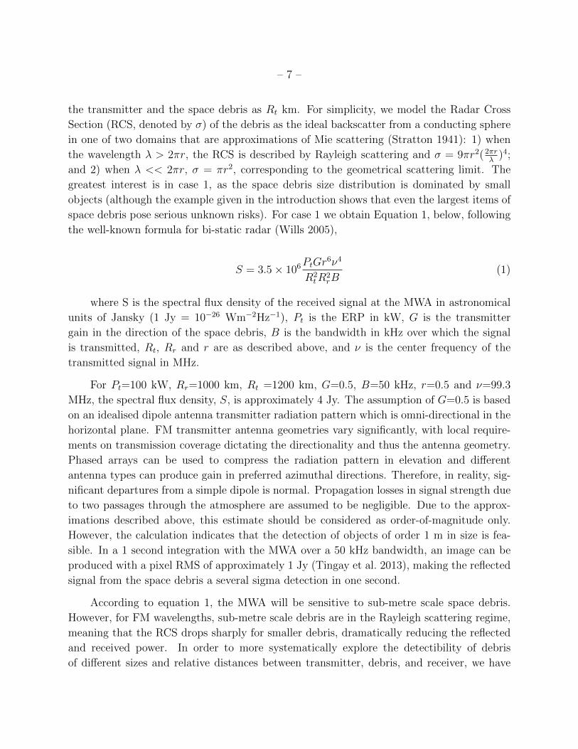
Figure 1 shows a selection of results from the simulations, for the Perth-based 6JJJ

transmitter and the ranges of debris size and altitudes listed above. Also shown is a single

point representing the result of the simple calculation from Equation 1. The simple cal-

culation overestimates, by a factor of approximately two, relative to the XFdtd simulation,

the flux density at the MWA. This level of agreement is reasonable, given the simplifying

assumptions made for Equation 1.

Figure 1 shows that debris with r > 0.5 m can plausibly be detected up to altitudes of

approximately 800 km with a one second observation. The solid line in Figure 1 denotes the

one sigma sensitivity calculation made for the simple example, above, based on information

from Tingay et al. (2013), showing that a three sigma detection can be made for debris

of r =0.5 m at 800 km. Of course, if longer observations can be utilised, the detection

thresholds can be reduced. For example, a ten second observation would yield a three sigma

detection of debris with r = 0.5 m at 1000 km.

The solution to the detection of smaller (∼10 cm) scale debris with low frequency passive

radar in the past has been to use ERPs of gigawatts, as with the 217 MHz NAVSPACECOM

“Space Fence” (Petersen 2012). An alternative approach is to build larger and more sensitive

receiving antennas. The natural evolution of the MWA is the much larger and more sensitive

4http://www.remcom.com/xf7

– 9 –

low frequency SKA, which will have a factor of ∼1000 more receiving area and be far more

sensitive than the MWA. The low frequency SKA may have great utility for space debris

tracking later this decade.

3. Verification of the technique

We verified the technique outlined above with an observation using the MWA during its

commissioning phase. This is a subarray of 32/128 tiles with a maximum east-west baseline

of roughly 1 km and a maximum north-south baseline of roughly 2 km, giving a synthesized

beam of roughly 5′ × 10′ at a frequency of ∼100 MHz. We observed an overflight of the

International Space Station (ISS) on 2012 November 26, as shown in Figure 2. The center

frequency of our 30.72 MHz bandpass was 103.4 MHz, and we correlated the data with a

resolution of 1 s in time and 10 kHz in frequency. We used two different array pointings, as

plotted in the right panel of Figure 2. The first was from 12:20:00 UT to 12:24:56 UT and

was pointing at an azimuth of 180◦ (due south) and an elevation of 60◦. The second was

from 12:24:56 UT to 12:29:52 UT at an azimuth of 90◦ (due east) and an elevation of 60◦.

As discussed in Tingay et al. (2013) and verified by Williams et al. (2012), the MWA has

an extremely broad primary beam (roughly 35◦ FWHM) which was held fixed during each

observation. We observed the overflight of the ISS between 12:23:00 UT and 12:26:00 UT,

when it was at a primary beam gain of > 1%, traversing about 112◦ on the sky.

During the pass, the ISS ranged in distance between approximately 850 km (at the low

elevation limit of the MWA, approximately 30◦) and approximately 400 km (near zenith at

the MWA) (Figure 2); its angular speed across the sky is approximately 0.5◦ per second,

corresponding to approximately five synthesised beams with this antenna configuration.

To image the data, we started with an observation pointed at the bright radio galaxy

3C 444 taken before the ISS observations. This observation was used as a calibration obser-

vation, determining complex gains for each tile assuming a point-source model of 3C 444,

which was sufficient to model the source given that its extent (< 4′) is the same as the

FWHM of the synthesised beam of the MWA subarray at this frequency. While we changed

pointings between this observation and those of the ISS, we have previously found that the

instrumental phases are very stable across entire days, and that only the overall amplitudes

need to be adjusted for individual observations.

Antenna-based gain solutions were obtained using the CASA task bandpass on a 2-

minute observation. Solutions were obtained separately for each 10 kHz channel, integrating

over the full two minutes. The flux density used for 3C 444 was 116.7 Jy at the central

– 10 –

frequency of 103 MHz, with a spectral index of −0.88. A S/N> 3 was required for a successful

per-channel, per-baseline solution, and the overall computed gain solutions for each antenna

were of S/N> 5. Calibration solutions were applied to the ISS observations using the CASA

task applycal and the corrected data were written to uv-fits format for imaging in miriad

(Sault, Teuben & Wright 1995).

For the two ISS observations, we flagged bad data in individual fine channels (10 kHz

wide) associated with the centers and edges of our 1.28 MHz coarse channels. Because of the

extremely fast motion of the ISS, we created images in 1 s intervals (the integration time used

by the correlator) using miriad. We started by imaging the whole primary beam (40◦×40◦),

separating the data into 3 × 10.24 MHz bandpasses. The bottom two bandpasses covered

the FM band, while the top bandpass was above the FM band. We used a 1′ cell size and

cleaned emission from Fornax A. Note that miriad does not properly implement wide-field

imaging, but our images used a slant-orthographic projection such that the synthesized beam

is constant over the image (Ord et al. 2010).

The results covering the two time intervals and two bandpasses are shown in Figure 3.

The ISS is readily visible as a streak moving through our images, but is only visible in

the images that cover the FM band as would be expected from reflected terrestrial FM

emission (as in McKinley et al. 2013). We predicted the position of the ISS based on its

two-line ephemeris (TLE) using the pyephem package5. The predicted position agrees with

the observed position to within the observational uncertainties.

To determine more quantitatively the nature of the emission seen in Figure 3, we im-

aged each 1 s interval and each 10 kHz fine channel separately (as before, this was done in

miriad). We did not deconvolve the images at all; most of them had no signal or the emis-

sion from the ISS was very weak. The emission from the ISS is not a point source (smeared

due to its motion) and adding deconvolution for a non-stationary object to our already

computationally-demanding task was not feasible. In each of our 180 × 3072 dirty images,

we located the position of the ISS based on its ephemeris. We then measured its flux density

by adding up the image data over a rectangular region of 10′ (comparable to our instrumen-

tal resolution) in width and with a length appropriate for the instantaneous speed of the

ISS (up to 40′ in a 1 s interval), as seen in Figure 4. The resulting dynamic spectra showing

flux density as functions of time and frequency are shown in Figure 5. These spectra have

been corrected for the varying primary beam gain of the MWA over its field-of-view based

on measurements of the sources PKS 2356−61 (first observation, assuming a flux density of

166 Jy at 97.7 MHz) and PKS J0237−1932 (second observation, assuming a flux density of

5http://rhodesmill.org/pyephem

– 11 –

35 Jy at 97.7 MHz); we have ignored the frequency-dependence of the primary beam gain for

the purposes of this calculation. Note that the emission seen in Figure 5 is manifestly not

radio-frequency interference (RFI) that is observed as a common-mode signal by all of our

tiles. It is only visible at a discrete point in our synthesized images corresponding to the

position of the ISS (Figure 4). We ran the same routines used to create the dynamic spectra

in Figure 5 but using a position offset from the ISS position, and we see almost no emission,

with what we do see consistent with sidelobes produced by bright emission in individual

channels, due to the ISS.

The ISS has an approximate maximum projected area of ∼1400 m2, is of mixed compo-

sition (thus not well approximated as perfectly conducting), has a highly complex geometry,

and was at an unknown orientation relative to the transmitter(s) and receiver during the

observations. The detailed transmitter antenna geometries and gain patterns are not known.

Thus, it is very difficult to accurately predict the flux density we would expect from either

simple calculations or electromagnetic simulations.

We can, however, unambiguously identify the origin of some of the transmissions re-

flected off the ISS. For example, we consider the dynamic spectrum from our observations in

Figure 5 at the time 12:24:20 UT. At this time there are clearly a number of strong signals

detected, plus a large number of much weaker signals. The five strongest signals at this time,

in terms of the integrated fluxes (Jy.MHz, measured by summing over individual transmitter

bands in the dynamic spectra to a threshold defined by the point at which the derivative

of the amplitude changed sign), are listed in Table 1, along with transmitters that can be

identified as the origin of the FM broadcasts (ACMA 2011). Each of the five identified trans-

mitters are local to Western Australia and, as can be seen from Figure 2, are all relatively

close to the ISS at this time. Each of the five transmitters have omni-directional antenna

radiation patterns in the horizontal plane.

If we take the reported ERP for a typical station from Table 1 and use it with Equation 1

to estimate the received flux, we find values of roughly 104 Jy.MHz, assuming the full 1400 m2

of reflecting area for the ISS. Given its varying composition and orientation, the measured

fluxes in Table 1 are reasonably consistent with this estimate.

Many, but not all, of the much weaker signals detected can also be identified. However,

it is clear that some of these weaker signals are from powerful transmitters at much larger

distances, making unique identification of the transmitter more difficult (FM broadcasts are

made on the same frequencies in different regions). Furthermore, it is clear that transmitters

local to Western Australia, and of comparable power to those listed in Table 1, have not

been detected in our observations. This is likely to be the result of the complex transmit-

ter/reflector/receiver geometries mentioned above and the rapid evolution of the geometry

– 12 –

# Freq. Flux Call sign(s) Location(s) ERP(s) Rt Rr

(MHz) (Jy.MHz) (kW) (km) (km)

1 98.1 3055 6JJJ Central Agricultural 80 537 489

2 96.5 1907 6NAM Northam 10 518 489

3 98.9 1799 6ABCFM/ Central Agricultural/ 80/10 537/498 489

6JJJ Geraldton

4 99.7 1718 6ABCFM/ Central Agricultural/ 80/10 537/498 489

6PNN Geraldton

5 101.3 1672 6PNN Geraldton 10 498 489

Table 1: The five strongest detected signals at 12:24:20 UT and transmitters identified with

those signals

with time, illustrated by the rapid evolution of the received signals identified in Table 1.

The five strongest signals at 12:24:20 UT are strongest over a 5 second period, have a highly

modulated amplitude over a further 30 second period, but are generally very weak or not

detected over the majority of our observation. Thus, it is highly likely that other transmit-

ters of comparable strength would be detected at other times, when favourable geometries

prevail. At 12:24:20 UT, it appears that the geometries were favourable for the Central

Agricultural, Northam and Geraldton transmitters, but not for transmitters of comparable

power in Perth, Bunbury and Southern Agricultural. We note that, while the strongest sig-

nals detected originated from transmitters with omni-directional transmitting antennas (see

above), the transmittors of comparable power not detected (Perth, Southern Agricultural

and Bunbury) also have omni-directional antennas. Thus, the most likely factor driving

detection or non-detection is the transmitter/reflector/receiver geometry, rather than trans-

mitting antenna directionality.

The modulation in power of the reflected radiation is likely at least partly due to “glints”

from the large, complex structure, which creates a reflected radiation pattern whose finest

angular angular scale is ∼ λ/d, where λ is the wavelength of the radiation and d is the extent

of the object. For d ∼ 100 m (full extent of the ISS) and λ ∼ 3 m, the glints are > 2◦ in

angular extent. At an altitude of ∼500 km, the smallest glint footprint on the surface of the

Earth is ∼ 10 km. With an ISS orbital speed of 8 kms−1, the glint duration at the MWA

is of order one second. This corresponds well to some of the modulation timescales seen in

Figure 5, although modulation exists on longer timescales (10 seconds and longer). These

longer timescales may be due to glints involving structures smaller than the full extent of the

ISS (single or multiple solar panels, for example). A full analysis of the modulation structure

of the signals is extremely complex and cannot be performed at a sufficiently sophisticated

level to be useful at present. In the future, detailed electromagnetic simulations of complex

– 13 –

reflector geometries may be used to gain insight into the modulations, but such an analysis

is beyond the scope of the current work.

In long integrations, such as required for Epoch of Reionisation experiments (Bowman

et al. 2013), the effect of having 10 pieces of space debris in the MWA primary beam at any

given time with flux densities >1 Jy is the equivalent of a <1 mJy additional confusion noise

foreground component in the FM band. This contribution will have no discernable impact

on the MWA’s science goals for observations in the FM band.

4. Discussion and future directions

At metre size scales, of order 1000 pieces of debris are currently known and tracked.

On average, up to approximately 10 such pieces will be present within the MWA field-of-

view at any given time, allowing continuous, simultaneous detection searches and tracking

opportunities.

These estimated detection rates naturally lead to two primary capabilities. The first is

a blind survey for currently unknown space debris, provided by the very large instantaneous

field-of-view of the MWA. The second capability is the high cadence detection and tracking

of known space debris. The wide field-of-view of the MWA means that large numbers of

debris can be simultaneously detected and tracked, for a substantial fraction of the time

that they appear above the local horizon.

Imaging with the MWA can provide measurements of the right ascension and declination

(or azimuth and elevation) of the space debris, as seen from the position of the MWA

(convertable to topocentric right ascension and declination). The MWA will also be able to

measure the time derivatives of right ascension and declination, giving a four vector that

defines the “optical attributable”. Measurements of the four vector at two different epochs

allow an estimate of the six parameters required to describe an orbit. Farnocchia et al.

(2009) describe methods for orbit reconstruction using the optical attributable, taking into

account the correlation problem (being able to determine that two measurements of the four

vector at substantially different times can be attributed to the same piece of space debris).

The calculations and practical demonstrations presented above show that the basic tech-

nique using the MWA is feasible and worthy of further consideration as a possible addition

to Australia’s SSA capabilities, particularly considering that the MWA is the Precursor to

the much larger and more sensitive low frequency SKA. However, the calculations and ob-

servational tests presented here also point to the challenges that will need to be met in order

to develop this concept into an operational capability.

– 14 –

Overall, these challenges relate to the non-standard nature of the imaging problem

for space debris detection, compared to the traditional approach for astronomy. In radio

interferomeric imaging, a fundamental assumption is made that the structure of the object

on the sky does not change over the course of the observation. This assumption is broken

in spectacular fashion when imaging space debris, due to their rapid angular motion across

the sky relative to background celestial sources and due to the variation in RCS caused by

the rapidly changing transmitter/reflector/receiver geometry.

Another standard assumption used in astronomical interferometric imaging is that the

objects being imaged lie in the far field of the array of receiving antennas; the wavefronts

arriving at the array can be closely approximated as planar. It transpires that for space

debris, most objects lie in the transition zone between near field and far field at low radio

frequencies, for an array the size of the MWA. Signal to noise is degraded somewhat when

the standard far-field assumption is adopted, as an additional smearing of the imaged ob-

jects results. It is worth noting that this will be a much larger effect for the SKA, with a

substantially larger array footprint on the ground. Thus, accounting for this effect for the

MWA will be an important step toward using the SKA for SSA purposes. For example,

for an object at 1000 km and the MWA spatial extent of 3 km, the deviation from the

plane wave assumption translates into more than a radian of phase error across the array at

a frequency of 100 MHz, which produces appreciable smearing of the reconstructed signal

with traditional imaging. It may be possible to use the near field nature of the problem to

undertake 3-dimensional imaging of the debris, using the wavefront curvature at the array

to estimate the distance to the debris.

Further significant work is required to implement modified signal and image processing

schemes for MWA data that take account of these time-dependent and geometrical effects

and sharpen the detections under these conditions. For example, the flexible approach

to producing MWA visibility data (the data from which MWA images are produced) allows

modifications to the signal processing chain to incorporate positional tracking of an object in

motion in real-time. Additionally, it is possible to collect data from the MWA in an even more

basic form (voltages captured from each antenna) and apply high performance computing

in an offline mode to account for objects in motion. This would also enable measurement of

the Doppler shifts of individual signals (expected to be ∼ few kHz, which is smaller than our

current 10 kHz resolution) that could enable separation of different transmitters at the same

frequency and unambiguous identification of transmitters (a Doppler shift pattern fixes a

one-dimensional locus perpendicular to the path of the reflecting object, so combining two

passes allows two-dimensional localizations). That in turn would help with constraining

– 15 –

the basic properties of the reflecting objects6. Finally, modifications to image processing

algorithms can be applied in post-processing to correct for near-field effects, essentially a

limited approximation of the same algorithms that can be applied earlier in the signal chain.

The results of this future work will be reported in subsequent papers.

Once these improvements are addressed, the remaining significant challenges revolve

around searching for and detecting signals from known and unknown space debris. These

challenges are highly aligned with similar technical requirements for astronomical applica-

tions, in searches for transient and variable objects of an astrophysical nature. A large

amount of effort has already been expended in this area by the MWA project, as one of the

four major science themes the project will address (Bowman et al. 2013; Murphy et al. 2013).

To illustrate the challenges, our flux estimates require (for example) greater than 4σ signif-

icance, but that is for a single trial. This is correct when looking to recover debris with an

approximately known ephemeris, but blind searches have large trial factors that can require

significantly revised thresholds. Given the full 2400 deg2 field-of-view of the MWA, we must

search over ∼ 104 individual positions in each image to identify unknown debris. Combined

with 3000 channels and 3600 time samples (for an hour of observing; note that we might

observe with a shorter integration time in the future) this results in 1011 total trials. So

our 4σ threshold (which implies 1 false signal in 104 trials) would generate 107 false signals,

and we would need something like an 8σ threshold to be assured of a true signal. Given

the steep dependence of flux on object size (Equation 1) this means our size limit may need

to be increased significantly. However, knowledge of individual bright transmitters (from

the type of analysis presented in this paper) means we can reduce the number of trials in

the frequency axis substantially, and seeking patterns among adjacent time samples that fit

plausible ephemerides will also help mitigate this effect.

If the challenges above can be addressed and a robust debris detection and tracking

capability can be established with the MWA, it could become a very useful element of a

suite of SSA facilities focussed on southern and eastern hemispheric coverage centered on

Australia.

In November 2012 an announcement was made via an Australia-United States Ministe-

rial Consultation (AUSMIN) Joint Communique that a US Air Force C-band radar system

6Given the changing geometry between passes, more than two might be required before a given trans-

mitter is identified more than once with sufficient signal-to-noise for localization. Conversely, if the Doppler

measurement is sufficiently significant and the transmitter is sufficiently isolated, a single one-dimensional

localization might be enough for unique identification. We intend to test these ideas with future observations.

– 16 –

for space debris tracking would be relocated to Western Australia7. This facility will provide

southern and eastern hemispheric coverage, allowing the tracking of space debris to a 10 cm

size scale. This system can produce of order 200 object determinations per day (multiple sets

of range, range-rate, azimuth and elevation per object) and will be located near Exmouth in

Western Australia, only approximately 700 km from the MWA site.

Additionally, the Australian Government has recently made investments into SSA capa-

bilities, via the Australian Space Research Program (ASRP): RMIT Univerity’s “Platform

Technologies for Space, Atmosphere and Climate”; and a project through EOS Space Sys-

tems Pty Ltd, “Automated Laser Tracking of Space Debris”. The EOS project will result in

an upgrade to a laser tracking facility based at Mt Stromlo Observatory, near Canberra on

Australia’s east coast, capable of tracking sub-10 cm debris at distances of 1000 km8.

In principle, the C-band radar system, a passive radar facility based on the MWA, and

the laser tracking facility could provide a hierarchy of detection and tracking capabilities

covering the southern and eastern hemispheres. The C-band radar system could potentially

undertake rapid but low positional accuracy detection of debris, with a hand-off to the MWA

to achieve better angular resolution and rapid initial orbit determination (via long duration

tracks). The MWA could then hand off to the laser tracking facility for the most accurate

orbit determination. Such a diversity of techniques and instrumentation could form a new

and highly complementary set of SSA capabilities in Australia. A formal error analysis,

describing the benefits of combining the data from such a diverse set of tracking assets will

be the subject of work to be presented in a future paper.

Such a hierarchy of hand-off between facilities has implications for scheduling the MWA,

whose primary mission is radio astronomy. Currently the MWA is funded for science op-

erations at a 25% observational duty cycle (approximately 2200 hours of observation per

year). This duty cycle leaves approximately 6500 hours per year available to undertake SSA

observations (assuming that funds to operate the MWA for SSA can be secured). Even

taking a conservative approach where only night time hours are used for observation, up to

approximately 2200 hours could be available for SSA. It would be trivial to schedule regular

blocks of MWA time, per night or per week, to undertake SSA observations. Given the rapid

sky coverage of the MWA and the short observation times effective for SSA, the entire sky

could be scanned over the course of approximately one hour each night, or using multiple

shorter duration observations over the course of a night. Since the MWA can be rapidly

repointed on the sky, the possibility of interupting science observations for short timescale

7http://foreignminister.gov.au/releases/2012/bc mr 121114.html

8http://www.space.gov.au

– 17 –

follow-up SSA observations, triggered from other facilities such as the C-band radar, could

be considered.

A review of Australia’s capabilities in SSA was presented by Newsam & Gordon (2011),

pointing out that better connections between the SSA community and latent expertise and

capabilities in the Australian astronomical community could be leveraged for significant

benefit. In particular the authors suggested involving new radio astronomy facilities in SSA

activities, given the advances in Western Australia connected with the SKA. The develop-

ment of a passive radar facility in the FM band using the MWA would be a significant step

in this direction.

Immediate future steps are to repeat the ISS measurements with the full 128 tile MWA,

as an improvement on the 32 tile array used for the observations reported here, as well as to

target smaller known satellites as tests and to implement the improvements described above.

We acknowledge the Wajarri Yamatji people as the traditional owners of the Observa-

tory site. Support for the MWA comes from the U.S. National Science Foundation (grants

AST CAREER-0847753, AST-0457585, AST-0908884, AST-1008353, and PHY-0835713),

the Australian Research Council (LIEF grants LE0775621 and LE0882938), the U.S. Air

Force Office of Scientic Research (grant FA9550-0510247), the Centre for All-sky Astrophysics

(an Australian Research Council Centre of Excellence funded by grant CE110001020), New

Zealand Ministry of Economic Development (grant MED-E1799), an IBM Shared Univer-

sity Research Grant (via VUW & Curtin), the Smithsonian Astrophysical Observatory, the

MIT School of Science, the Raman Research Institute, the Australian National University,

the Victoria University of Wellington, the Australian Federal government via the National

Collaborative Research Infrastructure Strategy, Education Investment Fund and the Aus-

tralia India Strategic Research Fund and Astronomy Australia Limited, under contract to

Curtin University, the iVEC Petabyte Data Store, the Initiative in Innovative Computing

and NVIDIA sponsored CUDA Center for Excellence at Harvard, and the International Cen-

tre for Radio Astronomy Research, a Joint Venture of Curtin University and The University

of Western Australia, funded by the Western Australian State government. The electromag-

netic simulations were performed by Gary Bedrosian and Randy Ward of Remcom Inc.

Facility: MWA.

– 18 –

REFERENCES

The Radio and Television Broadcasting Stations Internet Edition, Commonwealth of Aus-

tralia, 2011. ISSN 1449-5686 (http://www.acma.gov.au)

Bowman, J. et al. 2013, PASA, 30, 31

Dempsey, P. et al. 2012, Committee on the Peaceful Uses of Outer Space Scientific and

Technical Subcommittee, Forty-ninth session (Vienna, 6-17 February 2012) Item 14

of the draft provisional agenda, long-term sustainability of outer space activities

(A/AC.105/C.1/2012/CRP.16)

Dewdney, P.E., Hall, P.J., Schlizzi, R.T & Lazio, T.J.L. 2009, IEEE, 97, 8, 1482

Farnocchia, D., Tommei, G., Milani, A. & Rossi, A. 2009, arXiv:0911.0149

Haslam, C. G. T, Salter, C. J., Stoffel, H. & Wilson, W. E. 1982, A&AS, 47, 1

Johnston, S. et al. 2008, Ex.A., 22, 151

McKinley, B. et al. 2013, AJ, 145, 23

Newsam, G. & Gordon, N. 2011, Conference Technical Papers of the 2011

Advanced Maui Optical and Space Surveillance Technologies Conference

(http://www.amostech.com/technicalpapers/2011.cfm)

Murphy, T. et al. 2013, PASA, 30, 6

Ord, S. M. et al. 2010, PASP, 122, 1353

Petersen, J.K. 2012, Handbook of Surveillance Technologies (3rd Edition), CRC Press

(Florida, USA) ISBN:978-1-4398-7315-1

Ruitz, Leushacke & Rosebrock 2005, Proceedings of the 4th European Conference on Space

Debris (ESA SP-587). 18-20 April 2005, ESA/ESOC, Darmstadt, Germany. Editor:

D. Danesy., p.89

Sault R.J., Teuben P.J., & Wright M.C.H. 1995. In Astronomical Data Analysis Software

and Systems IV, ed. R. Shaw, H.E. Payne, J.J.E. Hayes, ASP Conference Series, 77,

433

Stratton, J.A. 1941, Electromagnetic Theory, New York: McGraw-Hill

Tingay, S.J. et al. 2013, PASA, 30, e007

http://www.acma.gov.au

http://arxiv.org/abs/0911.0149

http://www.amostech.com/technicalpapers/2011.cfm

– 19 –

Technical Report on Space Debris, 1999, United Nations Publication, Sales No. E.99.I.17,

ISBN 92-1-100813-1

Welch, J. et al. 2009, IEEE, 97, 1438

Williams, C. L. et al. 2012, ApJ, 755, 47

Wills, N.J. 2005, Bistatic Radar, Scitech Publishing Inc. (North Carolina, USA) ISBN:1-

891121-45-6

This preprint was prepared with the AAS LATEX macros v5.2.

– 20 –

Fig. 1.— The results of electromagnetic simulations, as described in the text. These simula-

tions model the flux density at the MWA for space debris modelled as a perfectly conducting

sphere (0.2, 0.5, 1 and 10 m radii) at altitudes of 200, 400, 800 and 1600 km above the

MWA site, with a transmitter at 99.3 MHz based near Perth (∼700 km from the MWA).

Also shown is a single point representing the example calculation based on Equation 1, with

r = 0.5 m

– 21 –

12:23:00

12:24:00

12:25:00

12:26:00

12:24:20

MWA

Albany

BunburyCA

Geraldton

Broome

MerredinPerth

Meekatharra

Northam

Kalgoorlie

SA

Port Hedland

12:23:00

12:24:20

12:25:00

12:25:59

PKS 2153-69

PKS 0235-19

For A (double)

PKS 2356-61

LMC

Pic A

3C 444

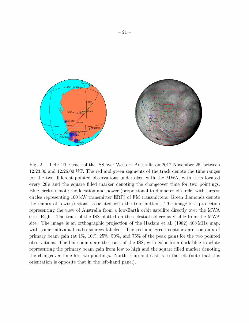
Fig. 2.— Left: The track of the ISS over Western Australia on 2012 November 26, between

12:23:00 and 12:26:00 UT. The red and green segments of the track denote the time ranges

for the two different pointed observations undertaken with the MWA, with ticks located

every 20 s and the square filled marker denoting the changeover time for two pointings.

Blue circles denote the location and power (proportional to diameter of circle, with largest

circles representing 100 kW transmitter ERP) of FM transmitters. Green diamonds denote

the names of towns/regions associated with the transmitters. The image is a projection

representing the view of Australia from a low-Earth orbit satellite directly over the MWA

site. Right: The track of the ISS plotted on the celestial sphere as visible from the MWA

site. The image is an orthographic projection of the Haslam et al. (1982) 408 MHz map,

with some individual radio sources labeled. The red and green contours are contours of

primary beam gain (at 1%, 10%, 25%, 50%, and 75% of the peak gain) for the two pointed

observations. The blue points are the track of the ISS, with color from dark blue to white

representing the primary beam gain from low to high and the square filled marker denoting

the changeover time for two pointings. North is up and east is to the left (note that this

orientation is opposite that in the left-hand panel).

– 22 –

Dec

linat

ion

12:25:13 FM 98.7-108.7 MHz

Right Ascension

12:25:14 FM 98.7-108.7 MHz

Right Ascension

12:25:13 FM 108.7-118.7 MHz

PKS J0237-1932

PKS J0200-3053Fornax A

12:25:14 FM 108.7-118.7 MHz

ISS

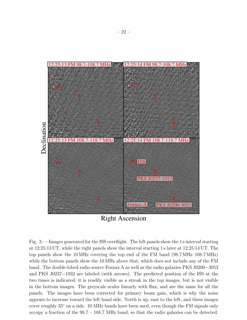
Fig. 3.— Images generated for the ISS overflight. The left panels show the 1 s interval starting

at 12:25:13 UT, while the right panels show the interval starting 1 s later at 12:25:14 UT. The

top panels show the 10 MHz covering the top end of the FM band (98.7 MHz–108.7 MHz)

while the bottom panels show the 10 MHz above that, which does not include any of the FM

band. The double-lobed radio source Fornax A as well as the radio galaxies PKS J0200−3053

and PKS J0237−1932 are labeled (with arrows). The predicted position of the ISS at the

two times is indicated; it is readily visible as a streak in the top images, but is not visible

in the bottom images. The greyscale scales linearly with flux, and are the same for all the

panels. The images have been corrected for primary beam gain, which is why the noise

appears to increase toward the left hand side. North is up, east to the left, and these images

cover roughly 35◦ on a side. 10 MHz bands have been used, even though the FM signals only

occupy a fraction of the 98.7 – 108.7 MHz band, so that the radio galaxies can be detected.

– 23 –

Dec

linat

ion

12:25:13 FM 98.7-108.7 MHz

Right Ascension

12:25:14 FM 98.7-108.7 MHz

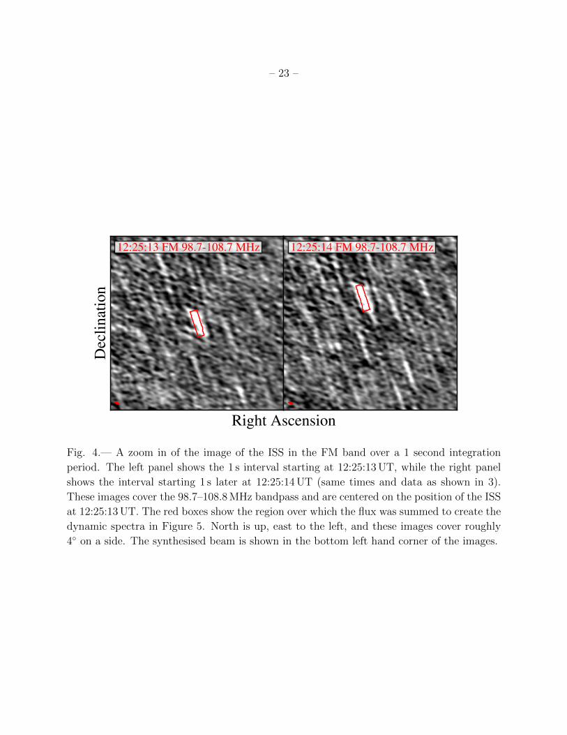
Fig. 4.— A zoom in of the image of the ISS in the FM band over a 1 second integration

period. The left panel shows the 1 s interval starting at 12:25:13 UT, while the right panel

shows the interval starting 1 s later at 12:25:14 UT (same times and data as shown in 3).

These images cover the 98.7–108.8 MHz bandpass and are centered on the position of the ISS

at 12:25:13 UT. The red boxes show the region over which the flux was summed to create the

dynamic spectra in Figure 5. North is up, east to the left, and these images cover roughly

4◦ on a side. The synthesised beam is shown in the bottom left hand corner of the images.

– 24 –

88 89 90 91 92 93 94 95 96 97 98Frequency (MHz)

12:23:0012:23:1012:23:2012:23:3012:23:4012:23:5012:24:0012:24:1012:24:2012:24:3012:24:4012:24:5012:25:0012:25:1012:25:2012:25:3012:25:4012:25:50

96.5

MH

z6N

AM

98 99 100 101 102 103 104 105 106 107 108Frequency (MHz)

12:23:0012:23:1012:23:2012:23:3012:23:4012:23:5012:24:0012:24:1012:24:2012:24:3012:24:4012:24:5012:25:0012:25:1012:25:2012:25:3012:25:4012:25:50

98.1

MH

z6J

JJ

99.7

MH

z6P

NN

/6A

BC

RN

101.

3M

Hz

6PN

N

98.9

MH

z6J

JJ/6

AB

CFM

Fig. 5.— Dynamic spectra over the time range 12:23:00 to 12:26:00 UT and over the fre-

quency ranges 88–98 MHz (top panel) and 98–108 MHz (bottom panel). The black regions

are those with no data, either because of the gap between the observations or the individual

channels flagged during imaging. The color scale in both images is the same and is linearly

proportional to flux density, with the white stretch indicating the strongest signals. The

specific time discussed in the text, 12:24:20 UT, is marked with a dashed line. Individual

FM frequencies from Table 1 are also labeled. The noisier portions at the beginning and

end of the first observation and at the end of the second observation are because the flux

densities have been corrected for the primary beam gain, which is low at those times.

on the detection and tracking of space debris using the

Documents