on the contravariant form of the navier–stokes...

Journal of Computational Physics 199 (2004) 355–375

www.elsevier.com/locate/jcp

On the contravariant form of the Navier–Stokes equationsin time-dependent curvilinear coordinate systems

Haoxiang Luo *, Thomas R. Bewley

Flow Control Lab, Dept. of MAE, UC San Diego, La Jolla, CA 92093-0411, USA

Received 30 July 2003; received in revised form 17 November 2003; accepted 14 February 2004

Available online 19 March 2004

Abstract

The contravariant form of the Navier–Stokes equations in a fixed curvilinear coordinate system is well known.

However, when the curvilinear coordinate system is time-varying, such as when a body-fitted grid is used to compute

the flow over a compliant surface, considerable care is needed to handle the momentum term correctly. The present

paper derives the complete contravariant form of the Navier–Stokes equations in a time-dependent curvilinear coor-

dinate system from the intrinsic derivative of contravariant vectors in a moving frame. The result is verified via direct

transformation. These complete equations are then applied to compute incompressible flow in a 2D channel with

prescribed boundary motion, and the significant effect of some terms which are sometimes either overlooked or assumed

to be negligible in such a derivation is quantified.

� 2004 Elsevier Inc. All rights reserved.

Keywords: Contravariant; Navier–Stokes equations; Time-dependent curvilinear coordinates

1. Introduction

The Navier–Stokes equations in a fixed curvilinear coordinate system were established long ago using

coordinate transformation; one may find the standard form of these equations and their derivation in

tensor calculus textbooks, see [1]. However, such a general form of the Navier–Stokes equations have not

been used widely in numerical simulations, since the calculation of the covariant derivatives in curvilinear

coordinate systems is generally quite expensive. Many researchers have opted for alternative forms of the

Navier–Stokes equations when they deal with flows in complex geometries via mapping into a regulardomain. Such an approach can also be applied to time-dependent curvilinear coordinate systems. For

example, a formulation is widely used in which Cartesian based velocity components multiplied by the

Jacobian of the transformation (i.e., the volume flux components) are used as the flow variables [2,3].

Another commonly used formulation incorporates the velocity vectors in both the Cartesian coordinate

*Corresponding author. Tel.: +1-858-822-3729; fax: +1-858-822-3107.

E-mail address: [email protected] (H. Luo).

0021-9991/$ - see front matter � 2004 Elsevier Inc. All rights reserved.

doi:10.1016/j.jcp.2004.02.012

mail to: [email protected]

356 H. Luo, T.R. Bewley / Journal of Computational Physics 199 (2004) 355–375

system and the curvilinear coordinate system [4–8]. In this formulation, though the contravariant velocity

vector is introduced to make the equations simpler, the acceleration of the momentum is ultimately de-

termined in the Cartesian coordinate directions. Voke and Collins [9] proposed a contravariant velocity–vorticity formulation of the Navier–Stokes equations for both compressible and incompressible flows in a

fixed general coordinate system. Their formulation avoids explicit use of the connection coefficients and the

transformation matrix elements in the governing equations at the expense of the computation of the

contravariant form of the vorticity.

Rosenfeld and Kwak [10] presented a discrete contravariant formulation of the incompressible Navier–

Stokes equations in generalized moving coordinates using a finite volume method that satisfies the geo-

metric conservation laws for time-varying computational cells. However, the corresponding PDE in the

continuous setting is not readily apparent from this inherently discrete formulation.Under some circumstances, for example, when the transformation is relatively simple, the use of the

continuous tensorial formulation of Navier–Stokes equations is manageable. Carlson et al. [11] extended

the tensorial formulation to the moving coordinate system case and used direct numerical simulation to

calculate turbulence in a channel with time-dependent wall geometries. Their formulation was used later by

Xu et al. [12] to simulate turbulent flow over a compliant surface. Because of the specific transformation

used in their work, a change in orientation of a vector into the new coordinate system is ascribed only to its

wall-normal component and many connection coefficients vanish. However, when deriving the temporal

derivative of a vector tensor in a moving frame, one has to be careful, since additional terms may appeardue to the moving coordinates. The derivation of Carlson et al. [11] omits some of these potentially im-

portant terms. Simply treating the temporal derivative of the contravariant form of the velocity vector in

the same way as for a scalar variable, such as density, fails to capture all of the terms in this formulation,

thereby possibly compromising the accuracy of the subsequent computations.

Ogawa and Ishiguro [13] also derived the temporal derivative of tensor vectors, as considered in the

present work, via a different approach than that used here, specifically, by considering the infinitesimal

geometric motion of the curvilinear coordinates. The form of the Navier–Stokes equations they ob-

tained, which is consistent with the present derivation, involves the covariant derivatives of the velocityof the coordinates that are missing in the analysis of Carlson et al. [11]. In the present work, we derive

the intrinsic temporal derivative of tensor vectors using an alternative approach, the quotient rule of

tensor analysis, and then obtain the complete contravariant form of the Navier–Stokes equations in

time-dependent curvilinear coordinate systems. Unlike the derivation of Ogawa and Ishiguro [13], which

is based on geometrical arguments, the tensor derivation given in the present paper may be easily

generalized to tensorial equations of order higher than one (vectors) if necessary. We also demonstrate

use of the equations by applying them to solve flows in 2D channels with moving boundaries. Note that,

in addition to approaches based on coordinate transformation, there are many other available tech-niques for computational fluid dynamics in systems with moving boundaries, e.g., volume tracking

methods, level-set methods, and immersed boundary methods, etc. Readers are referred to [14–16] for

more information.

2. Derivation of the Navier–Stokes equations in moving coordinate systems

2.1. Equations of motion in a fixed coordinate system

In order to introduce the notation to be used, we first consider a time-invariant transformation

xi ¼ xiðn1; n2; n3Þ from the Cartesian coordinates x to the curvilinear coordinates n. (Note that superscripts

indicate contravariant components, not powers, in the present notation.) We define the transformation

matrix

H. Luo, T.R. Bewley / Journal of Computational Physics 199 (2004) 355–375 357

C ¼ ox

on; cij ¼

oxi

onj; ð1Þ

and its inverse

�C ¼ on

ox; �cij ¼

oni

oxj: ð2Þ

The metric tensor and its inverse are defined by

gij ¼ cki ckj ; gij ¼ �cik�c

jk; ð3Þ

respectively. The Jacobian of the transformation is defined by

J ¼ jCj: ð4Þ

The transformation relationship between the contravariant velocity vector v in the Cartesian coordinate

system and its counterpart u in the curvilinear coordinate system is

vj ¼ cjiui; or ui ¼ �cijv

j: ð5Þ

The same relationship also applies to other contravariant vectors.

The mass and momentum conservation equations in contravariant form in a fixed coordinate system

may be written as follows [1, pp. 178–179]

oqot

þ ðquiÞ;i ¼ 0;

qoui

ot

�þ ujui;j

�¼ qf i þ T ij

;j ;

ð6Þ

where the contravariant vector f i is the external body force per unit mass and T ij is the contravariant stress

tensor. In the above equations, a comma with an index in a subscript denotes covariant differentiation:

ui;j ¼oui

onjþ Ci

jkuk; ð7Þ

where Cijk are the components of connection coefficients, also known as the Christoffel symbol of the second

kind. Now consider a time-dependent transformation from a Cartesian coordinate system x to a curvilinear

coordinate system n

xi ¼ xiðn1; n2; n3; sÞ;t ¼ s:

�ð8Þ

It is tempting (see, e.g., the derivations of Carlson et al. [11]) to simply apply the chain rule

o

ot! o

osþ onj

oto

onjð9Þ

and the relations (1)–(5) in order to re-express the temporal derivative terms in (6) and to cast it in the

moving coordinate system. But is this correct? The answer is not obvious for an equation as complicated as

(6). However, we may use a simple counterexample to show that such a simple substitution in fact misses

some terms which are sometimes important. Consider a uniform flow free from the external force. Its

velocity components in the Cartesian coordinate system are v1 ¼ 1, v2 ¼ v3 ¼ 0. Suppose we use the fol-

lowing coordinate transformation:


x1 ¼ n1 cos s� n2 sin s;x2 ¼ n1 sin sþ n2 cos s;

�C ¼ cos s � sin s

sin s cos s

� �; �C ¼ cos s sin s

� sin s cos s

� �; ð10Þ

which simply means that the new coordinate system is rotating counterclockwise at a constant speed. We

can see immediately [by (5)] that the velocity components in the new coordinate system are u1 ¼ cos s,u2 ¼ � sin s (the third component is neglected since this is a two-dimensional problem). Since u is inde-

pendent of n, and the connection coefficients Cijk are all zero, by (7) we have ui;j ¼ 0. However, applying (9)

would produce the momentum equation

oui

ot¼ oui

osþ onj

otoui

onj¼ oui

os¼ 0; ð11Þ

which is clearly incorrect. Apparently, the Coriolis force is not correctly accounted for in the rotating

coordinates by following this approach.

To solve the apparent dilemma, we examine the intrinsic temporal derivative of a tensor vector in a

moving frame and apply the differentiation to the contravariant velocity vector while using Reynolds’

transport theorem to derive correctly the desired form of the Navier–Stokes equations.

We shall rewrite the definition of Cijk, the Christoffel symbol of the second kind, to facilitate this deri-

vation. The common definition of the Christoffel symbol is given by

Cijk ¼ gip jk; p½ � ¼ 1

2gip

ogpjonk

�þ ogpk

onj� ogjk

onp

�;

where ½jk; p� is the Christoffel symbol of the first kind, as defined in [1, p. 162] by

jk; p½ � ¼ 1

2

ogpjonk

�þ ogpk

onj� ogjk

onp

�¼Xm

oxm

onpo

onjoxm

onk

� �� ¼ cmp

ocmkonj

:

The Christoffel symbol of the second kind may thus be written

Cijk ¼ gip jk; p½ � ¼ �cil�c

pl c

mp

ocmkonj

¼ �cildml

ocmkonj

¼ �ciloclkonj

: ð12Þ

2.2. The intrinsic derivative

We now follow the procedure in [1, p. 166] to derive the intrinsic derivative. Consider a time-dependent

coordinate transformation (8). The velocity vectors of the moving coordinates are

�Ui ¼ oxi

os; and Uj ¼ � onj

otð13Þ

in the Cartesian space and curvilinear space, respectively, and they satisfy the contravariant transformation

rule, i.e., �Ui ¼ cijUj.

Let �Bi be an arbitrary parallel covariant vector field with constant components in Cartesian space ðx; tÞ,and Bi be its covariant counterpart in the curvilinear space ðn; sÞ. Consider a curve describing the path of afluid particle, parameterized by xiðtÞ and niðtÞ in the two coordinate systems, respectively. Note that niðtÞcan be determined from xiðtÞ and the implicit function ni ¼ niðxj; tÞ implied by the transformation (8). The

two parametric equations xðtÞ and nðtÞ satisfy

dnk

dt¼ onk

otþ onk

oxpdxp

dt¼ �Uk þ �ckpv

p ¼ �Uk þ uk; ð14Þ


where vp ¼ dxp

dt and uk ¼ �ckpvp are the velocities of the particle in the Cartesian space and curvilinear space,

respectively. We are now looking for a derivative with respect to t, namely the intrinsic derivative, denoted

as DDt, which meets two requirements: (1) it should reflect the total variation of a tensor vector along the

curve due to infinitesimal change of t (correspondingly, in Cartesian coordinates, this derivative will reduce

to the material derivative), and (2) it should preserve tensor character so that it can be applied to any

coordinate system. By the first requirement, DBiDt should vanish along the curve, as Bi represents physically

the same constant parallel vector field as �Bi. Since we haveD�BiDt ¼

d�Bidt ¼ 0, which holds for all points along the

curve, this condition is

d�Bi

dt¼ d

dtð�cjiBjÞ ¼ �cji

dBj

dtþ Bj

d�cjidt

¼ 0: ð15Þ

Multiplying this equation by cir and summing over i, noting that cir�cji ¼ djr, we obtain the condition for the

covariant Br to be a parallel field,

dBr

dtþ Bjcir

d�cjidt

¼ 0: ð16Þ

This suggests that, for a covariant vector Br, the intrinsic derivative we are seeking is

DBr

Dt¼ dBr

dtþ Bjcir

d�cjidt

;

which indeed satisfies both requirements [fulfillment of the second requirement is seen from the derivation

of (16), noting that DBrDt ¼ cir

D�BiDt ]. In the same way, we may obtain a similar derivative for a parallel con-

travariant vector field.

More generally, we now use the quotient rule to derive the tensor character for such a derivative of an

arbitrary contravariant vector field. Switching dummy indices in (16) by i ! l, and then r ! i,

dBi

dt¼ �Bjcli

d�cjldt

¼ Bj �cjldclidt

� dcli�c

jl

dt

!¼ Bj �cjl

dclidt

�� ddji

dt

�¼ Bj�c

jl

dclidt

: ð17Þ

Now let Ai be any time-varying contravariant vector field in ðn; sÞ-space. Then AiBi and its derivative

along the curve nðtÞ, dðAiBiÞdt , are both scalars which are independent of the coordinate systems. However, by

(17)

d AiBið Þdt

¼ dAi

dtBi þ Ai dBi

dt¼ dAi

dtBi þ AiBj�c

jl

dclidt

¼ dAj

dt

�þ Ai�cjl

dclidt

�Bj: ð18Þ

Note that the dummy index i in the first term has been switched to j. Since dðAiBiÞdt is a scalar tensor and Bj is

an arbitrary covariant vector, the quotient rule implies that the term in brackets is a contravariant vector. It

is the intrinsic derivative we are seeking and may be written as

DAj

Dt¼ dAj

dtþ Ai�cjl

dclidt

: ð19Þ

Note that the material derivative ddt along the curve nðtÞ is

d

dt¼ o

osdsdt

þ o

onkdnk

dt¼ o

osþ o

onkdnk

dt: ð20Þ


Substitute (14) and (20) into (19), and the intrinsic derivative becomes

DAj

Dt¼ oAj

osþ oAj

onkdnk

dtþ Ai�cjl

oclios

�þ oclionk

dnk

dt

�¼ oAj

osþ oAj

onk

�þ Ai�cjl

oclionk

�dnk

dtþ Ai�cjl

oclios

¼ oAj

osþ oAj

onk

�þ Cj

kiAi

�dnk

dtþ Ai�cjl

oclios

¼ oAj

osþ Aj

;k uk�

� Uk�þ Ai�cjl

oclios

; ð21Þ

where the definition of Christoffel symbol of the second kind in (12) has been used. Furthermore, since

oclios

¼ o

osoxl

oni

� �¼ o

onioxl

os

� �¼ o �Ul

oni¼ oxk

onio �Ul

oxk¼ oxk

oni�Ul;k;

where the covariant derivative and partial derivative are the same in Cartesian space, and �Ul;k is actually a

mixed second order tensor, then

�cjloclios

¼ �cjlcki�Ul;k ¼ Uj

;i: ð22Þ

Finally, the intrinsic derivative of the contravariant vector Aj becomes

DAj

Dt¼ oAj

osþ Aj

;i uið � UiÞ þ AiUj

;i: ð23Þ

The additional terms that arise in the intrinsic temporal differentiation are due to the motion of the base

vectors which are also spatially varying. To see this let us consider a Cartesian vector

�a ¼ ajeðjÞ;

where the coefficient aj is the component of the contravariant counterpart of �a in the curvilinear coordinate

system ðn; sÞ, and eðjÞ is a set of Cartesian base vectors for ðn; sÞ-coordinates, defined by eiðjÞ ¼ oxi

onj¼ cij. The

derivative of �a with respect to t along the curve nðtÞ isd�a

dt¼ o�a

osþ o�a

onidni

dt¼ oaj

oseðjÞ þ aj

oeðjÞ

osþ oaj

onieðjÞ

�þ aj

oeðjÞ

oni

�dni

dt¼ oaj

os

�þ aiUj

;i þ aj;idni

dt

�eðjÞ; ð24Þ

where the definition of eðjÞ, Eqs. (12) and (22) have been used to showoeðjÞos ¼ Ui

;jeðiÞ andoeðjÞoni

¼ CkjieðkÞ, and the

dummy indices are swapped to complete the derivation. The expression in brackets is just the contravariant

form of the intrinsic derivative and shows that the additional terms come in with both the temporal and

spatial variability of the base vectors.

It should be pointed out this differentiation is not the same as the convective derivative, as described in[17] and [1, p. 185], which is used to study inherent material properties, especially for non-Newtonian flows,

even if our moving coordinates are chosen to be the material coordinates in which case the intrinsic de-

rivative reduces to DAj

Dt ¼ oAj

os þ AiUj;i. The convective derivative is simply oAj

os , which reflects the rate of change

of Aj in material coordinates. Note that the convective derivative oAj

os , when expressed in the fixed curvilinear

coordinates, has an involved form reminiscent of (23), but represents something different. The intrinsic

derivative DAj

Dt also takes into account the change caused by the motion of material coordinates themselves.

2.3. Equations of motion in a moving coordinate system

We now apply Reynolds’ transport theorem. Let F ðn; sÞ be any function and V ðtÞ be a closed volume

moving with the fluid. Then

D

Dt

Z Z ZV ðtÞ

F dV ¼Z Z Z

V ðtÞ

DFDt

�þ Fui;i

�dV ð25Þ


holds for any tensor F . If F is a scalar, e.g., F ¼ q, then the term AiUj;i in (23) does not exist and the co-

variant derivative reduces to the partial derivative, so we have DqDt ¼

oqot þ

oqoni

ðui � UiÞ. By the mass conser-

vation law we require the integration in (25) to vanish, and thus obtain the continuity equation

oqos

� oq

oniU i þ quið Þ;i ¼ 0; ð26Þ

which, incidentally, is exactly the same as what we get by replacing (9) into the mass conservation equation

in (6) in a fixed curvilinear coordinate system. The temporal terms in the energy conservation equation

transform in a similar manner.

If F ¼ qui is the momentum vector, by the definition of the intrinsic derivative in (23) and the mo-

mentum conservation law, we have

D

Dt

Z Z ZV ðtÞ

qui dV ¼Z Z Z

V ðtÞ

oqui

os

�þ ujð � UjÞ quið Þ;j þ qujUi

;j þ quiuj;j

�dV

¼Z Z Z

V ðtÞqf i�

þ T ij;j

dV : ð27Þ

Therefore the momentum conservation equation may be written

oui

osþ ujð � UjÞui;j þ ujUi

;j ¼ f i þ 1

qT ij;j : ð28Þ

Note that the continuity Eq. (26) has been substituted to make the above equation simpler.

When the n coordinate system is fixed, i.e., Uj ¼ 0, then the Eqs. (26) and (28) reduce to (6) as expected.

Conversely, however, the extra terms which arise from the temporal intrinsic differentiation of a tensor

vector, �Ujui;j þ ujUi;j, are not obviously seen in (6). Simply applying the chain rule (9) for temporal dif-

ferentiation in the momentum conservation equation in (6) instead produces �Uj oui

onj, which is not equiv-

alent to �Ujui;j þ ujUi;j.

2.4. Example: uniform flow in a rotating coordinate system

We now re-examine the example of the uniform flow in a spinning coordinate system, as introduced in

(10). The velocity of the spinning coordinate system is

U ¼ � on

ot¼ sin t � cos t

cos t sin t

� �x1

x2

� �¼ �n2

n1

� �:

Since the covariant differentiation reduces to partial differentiation in this case and ui;j ¼ 0, in this example

Eq. (28) reduces to

oui

osþ ujUi

;j ¼ 0;

which may be written

� sin s� cos s

� �þ 0 �1

1 0

� �cos s� sin s

� �¼ 0:

Thus, (28) is seen to hold in the present example.


2.5. Example: stagnation point flow in a material coordinate system

When Uj ¼ uj, that is, the velocity of the coordinate coincides with the velocity of the fluid, as Ogawaand Ishiguro [13] pointed out, Eqs. (26) and (28) become the expressions in Lagrange coordinates, or

material coordinates, which are often used to describe the mechanics of solids. We now consider the

problem of stagnation point flow where the Cartesian velocity components and pressure (divided by

the constant density) are given by, v1 ¼ ax1, v2 ¼ �ax2, p ¼ � a2

2½ðx1Þ2 þ ðx2Þ2�, and a is a constant scalar.

The velocity vector satisfies the Cartesian momentum equation which, in terms of the material derivative,

reduces to

dvi

dt¼ �di ¼ a2x1

a2x2

� �; ð29Þ

where �di is the contravariant pressure gradient vector divided by the density in Cartesian space. Motivated

by (29), we define the material coordinate system

n1 ¼ x1 e�at

n2 ¼ x2 eat;

�C ¼ eat 0

0 e�at

� �; �C ¼ e�at 0

0 eat

� �:

Note that in this special flow, the lines n1 ¼ constant remain parallel to the x2 axis and the lines

n2 ¼ constant remain parallel to the x1 axis though these lines move along with the fluid particles. Since

Uj ¼ uj, the contravariant form of the momentum conservation Eq. (28) in this example reduces to

oui

osþ ujUi

;j ¼ di; ð30Þ

where di denotes the counterpart of �di in the new coordinate system. Note that, by the definition of u, we

have

u ¼ U ¼ � on

ot¼ an1

�an2

� �;

and by the relationship between contravariant vectors we have

d ¼ �C�d ¼ a2n1

a2n2

� �;

so that, again, (28) is seen to hold in the present example.As it can be seen, in both examples, although the coordinate systems are orthogonal, the extra terms

arising from temporal differentiation of tensor vectors in a moving frame do not vanish.

3. Derivation by direct transformation

The Navier–Stokes equations in a time-dependent curvilinear coordinate system may also be obtained by

directly transforming the equations in Cartesian system using the chain rule, though this approach issomewhat cumbersome and does not shed any additional light on the derivation or its physical significance.

That is, taking the Cartesian-based momentum equation

ovi

otþ vk

ovi

oxk¼ �f i þ 1

qo�T ik

oxk; ð31Þ


where �f i and �T ik are the counterparts of f i and T ik respectively in Cartesian space, we may transform the

equation by applying chain rule to all the derivatives, substituting v with u, multiplying it by �cji and invoking

index summation. From a physical perspective, this means projecting the momentum equation into the newcoordinate system. We show here how the transformation of the temporal term is handled, which is the

term of interest in this paper.

�cjiovi

ot¼ �cji

ocikuk

os

�þ onl

otociku

k

onl

�¼ ouj

osþ �cji

ocikos

uk þ onl

ot�cji c

ik

ouk

onl

�þ �cji

ocikonl

uk�

¼ ouj

osþ ukUj

;k � Ul ouj

onl

�þ Cj

lkuk

�¼ ouj

osþ uiUj

;i � Uiuj;i: ð32Þ

Similarly, the inertial term becomes

�cji vk ov

i

oxk¼ uiuj;i: ð33Þ

Clearly, (32) and (33) add up to the left-hand side of (28).

4. Application: flow in a channel with moving walls

A practical example of the use of such coordinate transformation is to compute the flow in a channel

with moving walls. Consider first an incompressible flow in a periodic channel of length Lx whose two walls

slightly deform about their nominal locations (x2 ¼ 1 and x2 ¼ �1) continuously with respect to time, as

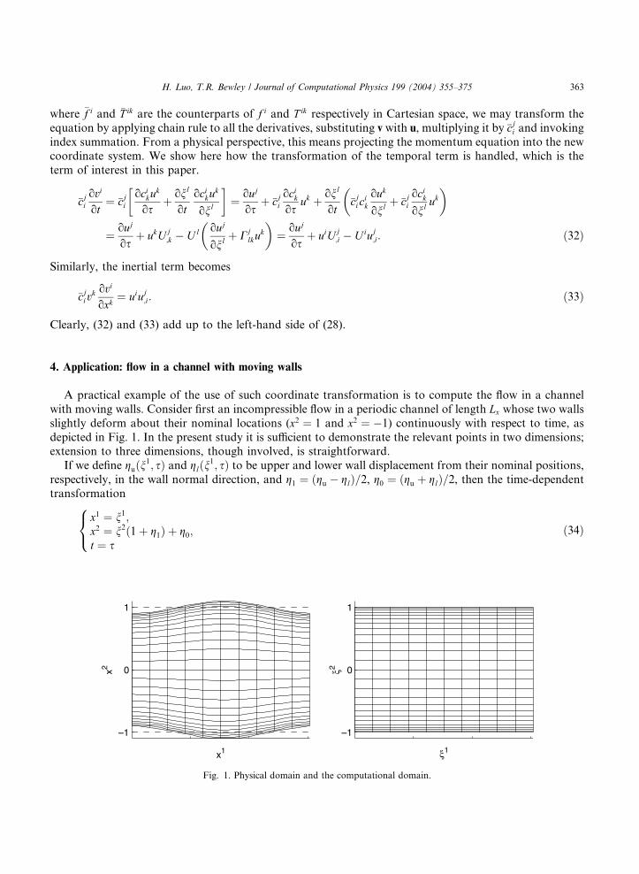
depicted in Fig. 1. In the present study it is sufficient to demonstrate the relevant points in two dimensions;extension to three dimensions, though involved, is straightforward.

If we define guðn1; sÞ and glðn1; sÞ to be upper and lower wall displacement from their nominal positions,

respectively, in the wall normal direction, and g1 ¼ ðgu � glÞ=2, g0 ¼ ðgu þ glÞ=2, then the time-dependent

transformation

x1 ¼ n1;x2 ¼ n2ð1þ g1Þ þ g0;t ¼ s

8<: ð34Þ

–1

0

1

x1

x2

–1

0

1

ξ1

ξ2

Fig. 1. Physical domain and the computational domain.


may be applied to transform the deformed domain into a rectangular domain. The time-independent

version of this transformation has been used by Gal-Chen and Somerville [18,19] to simulate the

meteorological phenomena of up-slope winds above a mountainous terrain. Carlson et al. [11] andKang and Choi [20] used the three-dimensional version of the transformation to calculate turbulence

in compliant channels. Note that conformal mapping or orthogonal transformation could be used to

solve the present two-dimensional test problem with significantly less effort. However, our main

purpose here is to illustrate a particular issue in general coordinate transformation on a 2D test

problem.

By definitions (1)–(4), we have (2� 2 instead of 3� 3 matrices are considered for this 2D problem)

C ¼1 0ox2

on1ox2

on2

� �; �C ¼

1 0

� 1J

ox2

on11J

� �;

J ¼ jCj ¼ ox2

on2¼ 1þ g1;

oni

ot¼ 0

� 1J

ox2

os

� �;

and the connection coefficients are

C1jk ¼ C2

22 ¼ 0;

C211 ¼

1

Jo2x2

oðn1Þ2¼ 1

1þ g1n2

o2g1oðn1Þ2

þ o2g0oðn1Þ2

!;

C212 ¼ C2

21 ¼1

Jo2x2

on1on2¼ 1

1þ g1

og1on1

:

To simplify the notation, we define the following non-constant transformation coefficients

u1 ¼on2

ox1¼ � 1

Jox2

on1¼ � 1

1þ g1n2

og1on1

�þ og0on1

�;

u2 ¼on2

ox2¼ 1

J¼ 1

1þ g1;

us ¼on2

ot¼ � 1

Jox2

os¼ � 1

1þ g1n2

og1os

�þ og0

os

�:

The two components of the momentum Eq. (28) may be written, after some manipulations, as

ou1

osþ us

ou1

on2þ u1

ou1

on1þ u2

ou1

on2¼ � 1

qop

on1

�þ u1

op

on2

�

þ mo

on1

�"þ u1

o

on2

�o

on1

�þ u1

o

on2

�u1 þ u2

2

o2u1

oðn2Þ2

#� Px;


ou2

osþ us

ou2

on2�u1

ous

on1� u2

ous

on2|fflfflfflfflfflfflfflfflfflfflfflfflffl{zfflfflfflfflfflfflfflfflfflfflfflfflffl}þu1ou2

on1þ u2

ou2

on2þ u1u2

2

JoJ

on1þ u1u1

1

Jo2x2

oðn1Þ2

¼ � 1

qu1

op

on1

�þ u1

op

on2

�� 1

qu2

2

op

on2� u1Px þ mu2

o

on1

�"þ u1

o

on2

�o

on1

�þ u1

o

on2

�Ju2� �

þ u22

o2Ju2

oðn2Þ2þ u1s1 þ 2

ou1

on1s2 þ 2

ou1

on2s3

#; ð35Þ

where m is the kinematic viscosity, Px is the uniform streamwise (x1-direction) pressure gradient that

maintains the bulk flow, and

s1 ¼o

on1

�þ u1

o

on2

�s2;

s2 ¼o2x2

oðn1Þ2þ u1

oJ

on1;

s3 ¼ u1s2 þ u22

oJ

on1:

By applying the metric invariants of the coordinate transformation, we may also express the conservative

form of the momentum equation (see Appendix, Eq. (A.1)), which is preferable for implementation in a

numerical algorithm.

In the particular transformation shown above, applying (9) would cause the two under-braced terms

�u1 ous

on1� u2 ous

on2in the u2 momentum equation in (35) to be absent. The continuity equation and boundary

conditions are given in the Appendix.

4.1. Numerical algorithm

To solve (35), the volume flux components q1 ¼ Ju1, q2 ¼ Ju2, and the modified pressure �p ¼ Jp=q are

chosen as the primitive variables. The numerical algorithm is based on that in [21,22]. The grid is chosen to

be evenly spaced in the streamwise direction (n1) and non-staggered so that Fourier transformation tech-

niques may be used to compute spatial derivatives in this direction. In the wall-normal direction (n2) thegrid is staggered and stretched using a hyperbolic tangent function allowing the near-wall region to bebetter resolved. Spatial derivatives of this direction is discretized using the second order centered finite

difference scheme.

The flow is advanced in time using a low-storage third-order Runge–Kutta method. At each Runge–

Kutta substep, all terms involving n1 derivatives and cross derivatives of the primitive variables are treated

explicitly, and all terms involving only n2 derivatives of the primitive variables are treated with an implicit

Crank–Nicholson method.

At the beginning of a time step, a full pressure equation is solved with a Neumann boundary condition

that is derived by imposing the discrete continuity constraint upon the discrete momentum equation. Atthe end of each Runge–Kutta substep, a projection function is solved to bring the velocity field to be

solenoidal and to update the pressure. Readers are referred to the Appendix for the details of this nu-

merical method.


To maintain the constant bulk velocity Ubulk (which is normalized by the nominal domain size), the

uniform streamwise pressure gradient Px is computed by integrating the u1 momentum equation over the

entire domain,

Ubulk ¼1

2Lx

Z 1þgu

�1þgl

Z Lx

0

v1 dx1 dx2 ¼ constant

) Px ¼1

2RJ dn1

Z �� u1�p þ mu1

ou1q1

on2þ mu2

2

oq1

on2

�n2¼1

n2¼�1

dn1:

ð36Þ

The discrete numerical integration scheme in the code exactly conserves both mass and momentum. By

computing Px with (36), constant mass flux is numerically guaranteed. The Reynolds number is thus based

on the bulk volume flux

Re ¼ Uchm

¼ 3

2

Ubulkhm

;

where Uc ¼ 32Ubulk is the centerline velocity of the corresponding Poiseuille flow with the same mass flux,

and h ¼ 1 is the half channel width. Time is normalized by hUc.

4.2. Laminar steady flow in channels with sinusoidal walls

The first case considered is the laminar flow in a symmetric channel with sinusoidal walls, as depicted inFig. 1, with gl ¼ �gu ¼ e cosðn1Þ. This case, though not addressing the problem of a moving coordinate

system, validates the correctness of the present code against an analytic result in the case of a stationary

coordinate system. The parabolic laminar profile in an unperturbed channel is used as the initial condition.

The wall deformation starts to grow gradually until the final geometry is reached and then remains un-

changed, and the simulation continues until the steady state is reached. The results are compared with that

from Tsangaris and Leiter [23], who solved the laminar steady flow in sinusoidal channels for Reynolds

numbers far above that for creeping flow. In their work, a perturbation method is used with the wall

amplitude e as the perturbation parameter. The stream function is expanded in a series, and the first-ordervariation is derived, which boils down to solving numerically a linear system of 4th-order differential

equations with two unknown functions and with variable coefficients.

Figs. 2 and 3 show the comparison of the Cartesian velocity components (v1 and v2) profiles for e ¼ 0:1and e ¼ 0:2 at Reynolds numbers Re ¼ 1:0; 10; 75; 200; 400. In our simulations, the number of Fourier

modes is 32� 64 in the n1 and n2 directions, respectively (i.e., 48� 64 dealiased collocation points), and the

length of the computational domain is Lx ¼ 2p. The resolution was doubled in both directions and the

calculations repeated with no significant change of the results.

The comparisons show that our simulations agree very well with the results obtained by Tsangaris andLeiter when both the wall deformation parameter e and the Reynolds number Re are small. However, the

discrepancies become more evident as e or Re is increased. The influence of e is expected because the

perturbation analysis of Tsangaris and Leiter is less accurate when the perturbation parameter e is in-

creased. The influence of Re is also expected since the leading-order truncation error from the perturbation

series is related to Reynolds number as well.

Our simulations also show that the critical Reynolds number for flow separation to happen at e ¼ 0:2 is

about Recrit ¼ 171, and the separation point is about n1 ¼ 2:6 which is slightly upstream the maximum

width of the wavy wall of the channel. These are slightly different from what Tsangaris and Leiter predicted,where Recrit ¼ 185 and the separation point is about n1 ¼ 2:4. As Reynolds number is increased above Recrit,separation regions in the diverging portion of the channel are formed, as illustrated in Fig. 4.

0 1 2 3 4 5 6 70

0.5

1v1 = 1

0 1 2 3 4 5 6 70

0.5

1v2 = 0.05

0 1 2 3 4 5 6 70

0.5

1

0 1 2 3 4 5 6 70

0.5

1

0 1 2 3 4 5 6 70

0.5

1

0 1 2 3 4 5 6 70

0.5

1

0 1 2 3 4 5 6 70

0.5

1

0 1 2 3 4 5 6 70

0.5

1

0 1 2 3 4 5 6 70

0.5

1

0 1 2 3 4 5 6 70

0.5

1

Re = 1.0

Re = 10

Re = 75

Re = 400

Re = 200

Fig. 2. Cartesian velocity profiles at various cross sections (x1 ¼ 0; 1; 2; 3; 4; 5; 6) of the channel for steady flow with e ¼ 0:1 and various

Reynolds numbers. Left: v1 component; Right: v2 component. Solid: numerical results; dashed: perturbation analysis.


4.3. Moving boundary simulation

To illustrate the important effects of the sometimes-neglected terms in the Navier–Stokes equations in

time-dependent curvilinear coordinates, we simulate the laminar flow in a channel with an oscillatingGaussian protuberance at center of the lower wall and corresponding blowing/suction applied at the op-

posite wall. The wall deformation is prescribed by

glðn1; tÞ ¼ e sin xtð Þ exp"�ðn1 � Lx

2Þ2

r2

#;

where e is the amplitude of the wall deformation, x is the oscillation frequency, and r is a constant de-termining the width of the protuberance.

To maintain the incompressibility of the flow, the upper wall is made porous and the velocity of the fluid

through the upper wall is identical to the velocity of the lower wall. In all tests of this section, the channel

length is chosen to be Lx ¼ p, Reynolds number is Re ¼ 200, and the wall deformation parameters are

e ¼ 0:1 and r ¼ 0:2. In the simulation, the number of Fourier modes is 42� 84 in the n1 and n2 directionsrespectively (i.e., 64� 84 dealiased collocation points) and the time step is 0:01. The time step was reduced

by a factor of 10 and there was no significant change of the results.

Due to the oscillation of the boundary, this flow exhibits time-periodic behavior. Fig. 5 shows both theinstantaneous streamlines’ and pressure’s oscillating patterns at different time phases within one period

0 1 2 3 4 5 6

–1

–0.5

0

0.5

1

Fig. 4. The streamlines for the case with e ¼ 0:2 and Re ¼ 400 showing the separation regions of the flow field.

0 1 2 3 4 5 6 70

0.5

1v1 = 1

0 1 2 3 4 5 6 70

0.5

1v2 = 0.05

0 1 2 3 4 5 6 70

0.5

1

0 1 2 3 4 5 6 70

0.5

1

0 1 2 3 4 5 6 70

0.5

1

0 1 2 3 4 5 6 70

0.5

1

0 1 2 3 4 5 6 70

0.5

1

0 1 2 3 4 5 6 70

0.5

1

0 1 2 3 4 5 6 70

0.5

1

0 1 2 3 4 5 6 70

0.5

1

Re = 1.0

Re = 10

Re = 75

Re = 200

Re = 400

Fig. 3. Cartesian velocity profiles at various cross sections (x1 ¼ 0; 1; 2; 3; 4; 5; 6) of the channel for steady flow with e ¼ 0:2 and various

Reynolds numbers. Left: v1 component; Right: v2 component. Solid: numerical results; dashed: perturbation analysis.


0 0.5 1 1.5 2 2.5 3–1

–0.5

0

0.5

1

0 0.5 1 1.5 2 2.5 3–1

–0.5

0

0.5

1

0 0.5 1 1.5 2 2.5 3–1

–0.5

0

0.5

1

0 0.5 1 1.5 2 2.5 3–1

–0.5

0

0.5

1

0 0.5 1 1.5 2 2.5 3–1

–0.5

0

0.5

1

0 0.5 1 1.5 2 2.5 3–1

–0.5

0

0.5

1

t = 0.1 t = 0.5 t = 1.0

t = 1.5 t = 2.0 t = 2.5

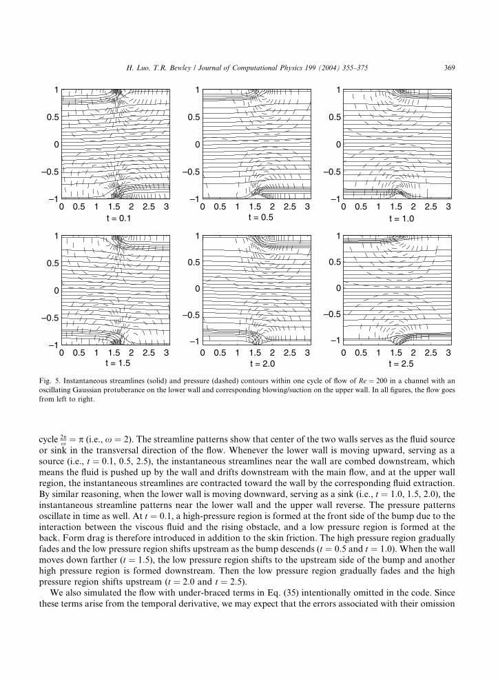
Fig. 5. Instantaneous streamlines (solid) and pressure (dashed) contours within one cycle of flow of Re ¼ 200 in a channel with an

oscillating Gaussian protuberance on the lower wall and corresponding blowing/suction on the upper wall. In all figures, the flow goes

from left to right.


cycle 2px ¼ p (i.e., x ¼ 2). The streamline patterns show that center of the two walls serves as the fluid source

or sink in the transversal direction of the flow. Whenever the lower wall is moving upward, serving as a

source (i.e., t ¼ 0:1, 0:5, 2:5), the instantaneous streamlines near the wall are combed downstream, which

means the fluid is pushed up by the wall and drifts downstream with the main flow, and at the upper wallregion, the instantaneous streamlines are contracted toward the wall by the corresponding fluid extraction.

By similar reasoning, when the lower wall is moving downward, serving as a sink (i.e., t ¼ 1:0, 1:5, 2:0), theinstantaneous streamline patterns near the lower wall and the upper wall reverse. The pressure patterns

oscillate in time as well. At t ¼ 0:1, a high-pressure region is formed at the front side of the bump due to the

interaction between the viscous fluid and the rising obstacle, and a low pressure region is formed at the

back. Form drag is therefore introduced in addition to the skin friction. The high pressure region gradually

fades and the low pressure region shifts upstream as the bump descends (t ¼ 0:5 and t ¼ 1:0). When the wall

moves down farther (t ¼ 1:5), the low pressure region shifts to the upstream side of the bump and anotherhigh pressure region is formed downstream. Then the low pressure region gradually fades and the high

pressure region shifts upstream (t ¼ 2:0 and t ¼ 2:5).We also simulated the flow with under-braced terms in Eq. (35) intentionally omitted in the code. Since

these terms arise from the temporal derivative, we may expect that the errors associated with their omission


would be small if the wall motion is slow, but large if the wall motion is fast. Two comparisons are carried

out, one with oscillation frequency x ¼ 0:5, the other with x ¼ 4. The resulting instantaneous streamlines

and pressure contours at a phase of the oscillation are shown in Figs. 6 and 7. In the slow wall motion case,x ¼ 0:5, the calculations with the terms omitted approximate our correct results fairly well. However, in the

faster wall motion case, x ¼ 4, the effects of omitted terms in the calculations become more evident. In

Fig. 7, where the wall is moving upward, the streamlines appear to overshoot above the bump, and un-

dershoot downstream due to this omission. The pressure contours also become more irregular when the two

terms are absent from the calculation.

0 0.5 1 1.5 2 2.5 3–1

–0.5

0

0 0.5 1 1.5 2 2.5 3–1

–0.5

0

t = 3.0

Fig. 6. Effects of the sometimes-neglected terms in the Navier–Stokes equations on flow of Re ¼ 200 when wall oscillation is slow

(x ¼ 0:5). Time instance: t ¼ 3:0. Left: instantaneous streamlines w; Right: pressure contours. Solid: the correct results; dotted: results

with neglected terms. Quantification of error: kwerrork2=kwk2 ¼ 0:2%; maxXðwerrorÞ=kwk2 ¼ 0:5%; kperrork2=kpk2 ¼ 17%;

maxXðperrorÞ=kpk2 ¼ 35%.

0 0.5 1 1.5 2 2.5 3–1

–0.5

0

0 0.5 1 1.5 2 2.5 3–1

–0.5

0

t = 1.8

Fig. 7. Effects of the sometimes-neglected terms in the Navier–Stokes equations on flow of Re ¼ 200 when wall oscillation is fast

(x ¼ 4). Time instance: t ¼ 1:8. Left: instantaneous streamlines w; Right: pressure contours. Solid: the correct results; dotted: results

with neglected terms. Quantification of error: kwerrork2=kwk2 ¼ 1:6%; maxXðwerrorÞ=kwk2 ¼ 6:8%; kperrork2=kpk2 ¼ 15%;

maxXðperrorÞ=kpk2 ¼ 55%.


5. Conclusions

In time-dependent curvilinear coordinates, the temporal derivative of a tensor vector is more compli-cated than the temporal derivative of a scalar. From Eq. (23), we can see that, for a contravariant vector Aj,

its temporal intrinsic derivative involves its own covariant differentiation (Aj;iU

i) and the covariant differ-

entiation of the velocity of the coordinates (AiUj;i). Treating Aj as a scalar during time differentiation is

incorrect, as it drops some important terms. Since Uj;i ¼ �cjl

oclios as we have shown, and cli ¼ oxl

oniis actually the

component of the base vectors of the new coordinate system, the term AiUj;i arises because base vectors of

the new coordinates are moving. Generally, in a time-dependent coordinate system AiUj;i would not vanish

even if the coordinate lines are straight and/or orthogonal, as shown by the two examples in Sections 2.4

and 2.5.Assuming that the extra terms in question are small is only valid when the coordinate system is moving

sufficiently slowly. We have demonstrated that these terms are not always negligible by simulating in-

compressible flows in a two-dimensional channel with prescribed boundary motion.

Acknowledgements

The authors would like to thank Prof. Constantine Pozrikidis of UC, San Diego for his valuable sug-gestions and comments during the course of this work.

Appendix A. Numerical implementation

In primitive variables. i.e., the volume flux components q1 ¼ Ju1, q2 ¼ Ju2, and the modified

pressure �p ¼ Jp=q, the conservative form of governing Eq. (35) for the compliant channel can be

written as

oqi

osþ T iðqjÞ þ NiðqjÞ ¼ �Gið�pÞ þ mLiðqiÞ � P i; ðA:1Þ

where T iðqjÞ is the term involving us, NiðqjÞ is the convection term, Gið�pÞ is the pressure gradient term,

mLiðqiÞ is the diffusion term, and P i is the uniform pressure gradient term. They are given by

T 1 ¼ oq1us

on2;

T 2 ¼ oq2us

on2� q1

ous

on1� q2

ous

on2;

N 1 ¼ oq1q1u2

on1þ oq1q2u2

on2;

N 2 ¼ oq1q2u2

on1þ oq2q2u2

on2þ 2u2

2q1q2

oJ

on1þ u2

2q1q1

o2x2

oðn1Þ2;


G1 ¼ o�p

on1þ o�pu1

on2;

G2 ¼ u1

o�p

on1

þ o�pu1

on2

!þ u2

2

o�p

on2;

L1 ¼ o

on1

�þ ou1�

on2

�o

on1

�þ ou1�

on2

�q1� �

þ u22

o2q1

oðn2Þ2;

L2 ¼ o

on1

�þ u1

o

on2

�o

on1

�þ u1

o

on2

�q2� �

þ u22

o2q2

oðn2Þ2þ u2q

1s1 þ 2ou2q

1

on1s2 þ 2

ou2q1

on2s3;

P 1 ¼ JPx;

P 2 ¼ Ju1Px:

Weighted by J , the continuity equation is

Diqi ¼oq1

on1þ oq2

on2¼ 0; ðA:2Þ

where Di is the divergence operator. The boundary conditions are the no-slip and no-penetration boundary

conditions which can be expressed as

q1jn2¼�1 ¼ 0;

q2jn2¼þ1 ¼oguos

;

q2jn2¼�1 ¼oglos

:

ðA:3Þ

One exception in present work is the example of moving boundary with Gaussian protuberance where the

upper wall is made porous and the boundary condition for the upper wall is thus q2jn2¼þ1 ¼ q2jn2¼�1 ¼oglos .

A.1. Temporal discretization

The flow is marched in time with a low-storage third-order Runge–Kutta method based on the scheme

used by Akselvoll and Moin [21] and Bewley et al. [22]. In each of the three Runge–Kutta substeps

k ¼ 1; 2; 3, two fractional steps are used: (1) an intermediate flow field qi�is obtained by solving the mo-

mentum equation with some terms treated explicitly and some implicitly (Crank–Nicholson); (2) the ve-

locities qi�are projected to the divergence free space and the pressure is updated by the projection function.

Let the operator Ai represent the terms treated explicitly and Bi represent the terms treated implicitlywhere the subscripts simply indicate the operator components, not covariant components. The discretized

momentum equation may be written as

qi� � qi

k�1

ds¼ bk Biðqj

� Þ�

þ Biðqjk�1Þ�þ ckAiðqj

k�1Þ þ fkAiðqjk�2Þ þ 2bk Gið�pk�1Þ

�� P i

�; ðA:4Þ


where the explicit and implicit operators are given by

A1ðqjÞ ¼ md

dn1dq1

dn1

�þ du1q

1

dn2

�þ m

d

dn2u1

dq1

dn1

� �� dq1q1u2

dn1;

A2ðqjÞ ¼ md

dn1dq2

dn1

�þ u1

dq2

dn2

�þ mu1

d

dn2dq2

dn1

� �þ m u2q

1s1

�þ 2

ou2q1

on1s2 þ 2

ou2q1

on2s3

�� dq1q2u2

dn1

� u22q

1q1d

dn1dx2

dn1

� �þ q1

dus

dn1;

B1ðqjÞ ¼ md

dn2u1

du1q1

dn2

� �þ mu2

2

d

dn2dq1

dn2

� �� dq1q2u2

dn2� dq1us

dn2;

B2ðqjÞ ¼ mu1

d

dn2u1

dq2

dn2

� �þ mu2

2

d

dn2dq2

dn2

� �� dq2q2u2

dn2� 2u2

2q1q2

dJ

dn1� dq2us

dn2þ q2

dus

dn2;

and ddni

means the numerical differentiation. The Runge–Kutta coefficients used in the present computations

are:

b1 ¼4

15; b2 ¼

1

15; b3 ¼

1

6;

c1 ¼8

15; c2 ¼

5

12; c3 ¼

3

4;

f1 ¼ 0; f2 ¼ � 17

60; f3 ¼ � 5

12:

Note that, in the same way as in [21], the non-linear term q2q2 needs to be linearized for the present system

to be solvable.

To make the intermediate flow field divergence free, we solve a projection function for / ¼ �pk � �pk�1:

D/ ¼ 1

2bkdsdqi

�

dni;

where D is the Laplacian operator given by

D/ ¼ DiGið/Þ ¼ d

dn1d/

dn1

�þ d/u1

dn2

�þ d

dn2u1

d/

dn1

��þ d/u1

dn2

��þ u2

2

d

dn2d/

dn2

� �: ðA:5Þ

This Poisson equation is solved in Fourier space. Since the non-constant coefficients make the Laplacian

non-invertible, we split the operator into two parts and solve the equation iteratively,

~D/s ¼ d

dnid/s

dni

� �¼ RHSs�1 ¼ 1

2bkdsdqi

�

dni� D�

� ~D�ð/s�1Þ; ðA:6Þ

where s is the iteration index. After / converges, the volume flux components and pressure are updated by

qik ¼ qi

� � 2bkdsGið/Þ ðA:7Þ

and

�pk ¼ �pk�1 þ /: ðA:8Þ


A.2. Pressure equation

At the beginning of each time step, we solve a full pressure equation which is obtained by taking di-

vergence of the Eq. (A.1):

D�p ¼ Dið � T i � Ni þ mLiÞ: ðA:9Þ

Note that the divergence of the uniform pressure gradient vanishes, which is true (within the machine

accuracy) in the discrete case as well. The Laplacian D is the same as in (A.5), so the pressure equation is

solved with the same iteration strategy as that used in (A.6).

The grid is discretized with a hyperbolic tangent stretching function and staggered in the wall-normal

direction. q2 is assigned on the family of gridpoints j ¼ 0; 1; 2; . . ., where j ¼ 0 corresponds to the lower

wall, and q1, �p are assigned on the family of gridpoints j ¼ 12; 1þ 1

2; 2þ 1

2; . . ., where j ¼ 1

2is midway be-

tween j ¼ 0 and j ¼ 1, and so on. Neumann boundary conditions for pressure are derived by enforcing

continuity of the flow at the first interior gridpoint. We illustrate the procedure for the lower wall, n2 ¼ �1.The discrete q1 momentum at j ¼ 1

2and the discrete q2 momentum at j ¼ 1, in an explicit Euler scheme,

may be written as

q1� � q1

k�1

2bkds

j¼1

2

¼ ð � T 1 � N 1 � G1 þ mL1 � P 1Þ j¼1

2

q2� � q2

k�1

2bkds

j¼1

¼ ð � T 2 � N 2 � G2 þ mL2 � P 2Þ j¼1

;

ðA:10Þ

and the boundary condition for q2�is

q2� jj¼0 ¼ q2

k jj¼0: ðA:11Þ

Applying the discrete divergence operator to q� at j ¼ 12, that is,

Diqi�� jj¼1

2¼

dq1� jj¼1

2

dn1þ 1

h12

q2� jj¼1

�� q2

� jj¼0

�;

where h12is the distance between gridpoints j ¼ 0 and j ¼ 1, and requiring it to be zero, we have

� 1

2bkds

dq1k�1 jj¼1

2

dn1

þq2

k�1 jj¼1 � q2k�1 jj¼0

h12

!þ 1

2bkds

q2k jj¼0 � q2

k�1 jj¼0

h12

!

¼ d

dn1�� T 1 � N 1 � G1 þ mL1 � P 1

� j¼1

2

þ 1

h12

�h� T 2 � N 2 � G2 þ mL2 � P 2

� j¼1

þ N 2�

þ G2�

j¼0� N 2�

þ G2�

j¼0

i; ðA:12Þ

where the boundary nodes q2k�1 jj¼0 and N 2 þ G2ð Þjj¼0 have been introduced. Note that the expression in the

first parentheses on the left hand side vanishes since qk�1 is divergence free. We split (A.12) into two

equations:

0 ¼ d

dn1�� N 1 � G1

�jj¼1

2þ 1

h12

�h� N 2 � G2

�jj¼1 þ N 2

�þ G2

�jj¼0

i; ðA:13Þ


q2k � q2

k�1

2bkds

j¼0

þ h12

dT 1jj¼12

dn1

þ T 2jj¼1

!þ N 2jj¼0 ¼ �ðG2 þ P 2Þjj¼0 þ m h1

2

dL1jj¼12

dn1

þ L2jj¼1

!; ðA:14Þ

where h12

dP1jj¼1

2

dn1þ P 2jj¼1 ¼ P 2jj¼0 has been applied since P i is divergence free. Note that (A.13) has the form of

the simplified pressure equation, so it may treated as the Poisson equation (A.9) evaluated at j ¼ 12. Eq.

(A.14) may be used to compute G2jj¼0 which is the Neumann boundary condition for (A.9). Actually, by

realizing that in theory T i and Li are divergence free, we have

h12

dT 1jj¼12

dn1þ T 2jj¼1 � T 2jj¼0; h1

2

dL1jj¼12

dn1þ L2jj¼1 � L2jj¼0:

Therefore, (A.14) is essentially the q2 momentum equation evaluated at the lower boundary.

References

[1] R. Aris, Vectors, Tensors, and the Basic Equations of Fluid Mechanics, Prentice-Hall, Englewood Cliffs, NJ, 1962.

[2] P.D. Thomas, C.K. Lombard, Geometric conservation law and its application to flow computations on moving grids, AIAA J. 17

(10) (1979) 1030–1037.

[3] R. Hixon, Numerically consistent strong conservation grid motion for finite difference schemes, AIAA J. 38 (9) (2000) 1586–1593.

[4] T.H. Pulliam, J.L. Steger, Implicit finite-difference simulations of three dimensional compressible flow, AIAA J. 18 (2) (1980) 159–

167.

[5] R. Smith, W. Shyy, Computation of unsteady laminar flow over a flexible two-dimensional membrane wing, Phys. Fluids 7 (9)

(1995) 2175–2184.

[6] C. Sheng, L.K. Taylor, D. Whitfield, Multigrid algorithm for three dimensional incompressible high-reynolds number turbulent

flows, AIAA J. 33 (11) (1995) 2073–2079.

[7] Z. Lei, G. Liao, G.C. dela Pena, A moving grid algorithm based on the deformation method. In: Nobuyuki Satofuka (Ed.),

Computational Fluid Dynamics 2000: Proceedings of the First International Conference on Computational Fluid Dynamics,

ICCFD, Kyoto, Japan, July 10–14, 2000, Springer-Verlag, New York, 2001, pp. 711–716.

[8] B.R. Hodges, R.L. Street, On simulation of turbulent nonlinear free-surface flows, J. Comput. Phys. 151 (1999) 425–457.

[9] P.R. Voke, M.W. Collins, Forms of the generalized Navier–Stokes equations, J. Eng. Math. 18 (1984) 219–233.

[10] M. Rosenfeld, D. Kwak, Time-dependent solutions of viscous incompressible flows in moving co-ordinates, Int. J. Numer. Meth.

Fluids 13 (1991) 1311–1328.

[11] H.A. Carlson, G. Berkooz, J.L. Lumley, Direct numerical simulation of flow in a channel with complex time-dependent wall

geometries: a pseudospectral method, J. Comput. Phys. 121 (1995) 155–175.

[12] S. Xu, D. Rempfer, J. Lumley, Turbulence over a compliant surface: numerical simulation and analysis, J. Fluid Mech. 478 (2003)

11–34.

[13] S. Ogawa, T. Ishiguro, A method for computing flow fields around moving bodies, J. Comput. Phys. 69 (1987) 49–68.

[14] Wei Shyy, H.S. Udaykumar, M.M. Rao, R.W. Smith, Computational Fluid Dynamics with Moving Boundaries, Taylor and

Francis, Washington, DC, 1996.

[15] K.S. Sheth, C. Pozrikidis, Effects of inertia on the deformation of liquid drops in simple shear flow, Comput. Fluids 24 (2) (1995)

101–119.

[16] E.A. Fadlun, R. Verzicco, P. Orlandi, J. Mohd-Yusof, Combined immersed-boundary finite-difference methods for three-

dimensional complex flow simulations, J. Comput. Phys. 161 (2000) 35–60.

[17] J.G. Oldroyd, On the formulation of rheological equations of state, Proc. Roy. Soc. A 200 (1063) (1950) 523–541.

[18] T. Gal-Chen, R. Somerville, On the use of a coordinate transformation for the solution of the Navier–Stokes equations, J.

Comput. Phys. 17 (1975) 209–228.

[19] T. Gal-Chen, R. Somerville, Numerical solution of the Navier–Stokes equations with topography, J. Comput. Phys. 17 (1975)

276–310.

[20] S. Kang, H. Choi, Active wall motions for skin-friction drag reduction, Phys. Fluids 12 (12) (2000) 3301–3304.

[21] K. Akselvoll and P. Moin. Large eddy simulation of turbulent confined coannular jets and turbulent flow over a backward facing

step. Technical Report TF-63, Thermosciences Division, Dept. of Mech. Eng., Stanford University, 1995.

[22] T.R. Bewley, P. Moin, R. Temam, Dns-based predictive control of turbulence: an optimal benchmark for feedback algorithms, J.

Fluid Mech. 447 (2001) 179–225.

[23] S. Tsangaris, E. Leiter, On laminar steady flow in sinusoidal channels, J. Eng. Math. 18 (1984) 89–103.

on the contravariant form of the navier–stokes...

Documents