on the complexity of join dependenciescse.unl.edu/~choueiry/documents/gyssens86.pdf · on the...

On the Complexity of Join Dependencies

MARC GYSSENS University of Antwerp

In [IO] a method is proposed for decomposing join dependencies (jds) in a relational database using the notion of a hinge. This method was subsequently studied in [ll] and [El. We show how the technique of decompasiti”” can be used t” make integrity checking m”re efficient. It turns ““t that it is important t” find a decomposition that minimizes the “umber of edges of its largest element. We show that the decompositions obtained with the method described in (lo] are optimal in this respect. This minimality criterion leads ta the definition of the degree of cy&ity, which allows us t” classify jds and leads to the notion of n-cyel*i@, of which acyclicity is a special case for n = 2. We then show that, for a fixed value of n (which may be greater than 2). integrity checking can be performed in polynomial time provided we restrict ourselves t” n-cyclic jds. Finally, we generalize a well-known characterization for acyclic jds by proving that n-cyclicity is equivalent ta “n-wise consistency implies global consistency.” As a consequence, consistency checking can be performed in polynomial time if we restrict aurselves to n-cyclic jds, for a tired value of n, not necessarily equal t” 2.

Categories and Subject Descriptors: G.2.2 [Discrete Mathematics]: Graph Thea,-grqoh &o- rithm, trees; H.2.1 [Database Management]: Logical Design-normalform, schem andsu6sckm

General Terms: Algorithms, Design, Theory

Additional Key Words and Phrases: Decomposition, equivalence of constraints, hypergraph, integrity checking, join dependency, multivalued dependency, relational database model

1. INTRODUCTION

Functional [S], multivalued [7, 191, and the more general join dependencies [16] are fundamental in relational database theory [5]. In [9] it was postulated that in real-world databases the structure can he expressed hy a set of functional dependencies together with only one join dependency. Here we are not concerned with functional dependencies, and therefore we consider relations on which a single join dependency is defined.

Unfortunately, integrity checking for join dependencies (jds), that is, checking whether the relation still satisfies the constraint after an update, turns out to he NP-complete in general. However, integrity checking can be avoided, since the presence of a jd is a necessary and sufficient condition to decompose a relation into a set of smaller relations, one for each edge of the jd. When this approach is followed (which is most common in practice), we must only verify whether the

Author’s address: M. Gyssens, Department of Mathematics and Camputer Science, University of Antwerp, U.I.A., Universiteitsplei” 1, 2610 Antwerpen, Belgium. Permission to copy without fee all “I part of this material is granted provided that the copies are not made “I distributed for direct commercial advantage, the ACM copyright notice and the title of the publication and its date appear, and notice is given that copying is by permission of the Association for Computing Machinery. To copy otherwise, “I t” republish, requires a fee and/or specific permission. 0 1986ACM 0730.0301/8s/0300-oOs1$00.75

82 * Marc Gyssens

subrelations still represent the information of one common relation each time an update is performed on the subrelations. This is called consistency checking. Unfortunately, consistency checking too is NP-complete in general.

However, there exist polynomial algorithms for integrity and consistency checking in the case where only acyclic join dependencies are involved. It is well known that the so-called acyclic join dependencies are those jds that can be decomposed into a set of multivalued dependencies (mvds) [2, 3, 8, 9, lo]. An mvd is essentially a join dependency with two edges. Because of these desirable properties, we often try to design a database in such a way that the jd describing it is acyclic. In many cases, however, the initial design produces cyclic join dependencies. Several techniques have been proposed to “change” these cyclic jds into acyclic ones (e.g., attribute splitting [9]), but these techniques may have undesirable side effects (e.g., the loss of the close relationship between split attributes). In this paper we want to point out that it is not necessary to reject all cyclic jds in database design. Indeed, some cyclic jda can also be decomposed into a set of “less complicated” join dependencies, as is illustrated by the following example. Consider the join dependency:

J:ob w ac w bd w cd w de w dfw eg w fg. A possible decomposition of J is

(&de w df m eg w fg, abed m defg, ab m a~ m cd m bdefg).

Other cyclic jds are not decomposable at all in this sense, such as

ab m bc m cd m de m ef m fg m ga.

This suggests that some cyclic jds are “more cyclic” than other cyclic jds, that is, that there exist several levels of cyclicity for jds of which acyclicity is only the “lowest” one (apart from the trivial jds).

If we look at this problem from the point of view of integrity checking, we see that replacing a jd by a decomposition can make integrity checking more efficient, since the jds in a decomposition have by definition fewer edges than the original jd. It is important to make the number of edges of the join dependencies of the decomposition we wish to use to perform integrity checking as small as possible, since the time complexity of making a join is first and foremost determined by the number of relations that have to be joined. Therefore, we define the degree of cyclicity of a join dependency J as the minimum overall decompositions of J of the number of edges of the largest join dependency in that decomposition. In particular, we show that this minimum in each decomposition can be obtained with the method introduced in [lo]. Hence the decompositions thus obtained are optimal in this respect.

The degree of cyclicity also seems a natural tool to classify join dependencies in the sence we discussed above. We therefore say that a jd is n-cyclic if its degree of cyclicity is at most n. In this way we get a hierarchical classification of jds in which acyclic jds appear for n = 2. We show that integrity checking can be performed in polynomial time provided only n-cyclic jds are considered for a fixed value of n, not necessarily 2. ACM Transactions on Database system. Vol. 11. NO. 1. March 1986.

Complexity of Join Dependencies * 83

As said before, in practical situations, the presence of a jd will be used to decompose the relation on which it is defined in a set of smaller relations. With this approach, the problem of integrity checking is replaced by the problem of consistency checking. In the case of an acyclic jd, consistency checking can be performed in polynomial time since acyclicity is equivalent with “pair-wise consistency implies global consistency” [2, 3, 8, 91. The notion of n-cyclicity of which acyclicity is a special case for n = 2 suggests e generalization of this result. We show here that n-cyclicity is indeed equivalent to “n-wise consistency implies global consistency.” As a consequence, checking e decomposed database for global consistency can be done in polynomial time if one allows only n-cyclic join dependencies, for a fixed level of cyclicity n, which may be greater than 2. Hence in database design we have to restrict the jds that may occur to jds of a certain level of cyclicity, but not necessarily to acyclic jds.

This paper is organized es follows. In Section 2 we give some basic notions about join dependencies and their hypergraph representations, which we use extensively throughout this paper. Essential to our decomposition methodology is the notion of e hinge. A hinge is e set of edges of e hypergraph that satisfies certain properties. We define this notion in Section 3, in which we also describe our decomposition methodology. In Section 4 we give en overview of the most important properties of this decomposition methodology discussed in earlier papers. In Section 5 we define the degree of cyclicity of e join dependency and characterize this notion in terms of the structure of the join dependency itself. Again the notion of a hinge turns out to be important in this characterization. We show that our decomposition minimizes the number of components in its largest element. We also introduce n-cyclicity, and we show that integrity checking ten be performed in polynomial time, provided only n-cyclic jds ere considered, for a fixed value of n. Finally, in Section 6, we prove that n-cyclicity is equivalent to “n-wise consistency implies global consistency” and show that, es a consequence, consistency checking can he done in polynomial time, provided only n-cyclic jds are considered, for e fixed value of n.

2. NOTATION AND TERMINOLOGY

In this paper we consider a universal relation scheme R(Q) (or R if no ambiguity is possible) consisting of e set a of attributes, each associated with a domain of values. We essume that each domain is infinitely denumerahle (e.g., the set of nonnegative integers). In the sequel we denote single attributes by small letters, whereas sets of attributes are denoted by capital letters. If X and Y are sets of attributes, we write XY for X U Y. If a, b, c, are attributes, we write abc . . for (a, b, c, . .I. In particular, we do not distinguish between the attribute a and the set {a).

Let X C 0. A tuple t over X is a mapping that associates with each attribute a of R e value of its corresponding domain. An instance r over X is a set of tuples over X. Let Y C X and let t be a tuple over X. The projection oft onto Y, denoted t[ Y], is obtained by restricting t to the attributes of Y. If r is an instance over X, the set obtained by projecting each tuple of r onto Y is said to be the projection of r onto Y, denoted Q(T).

ACM T.ansaction. on DatabaseSystems, “0,. II, No. 1, March 1986.

a4 * Marc Gyssens

L&X, ,..., XhCQ.Wesaythat(r, ,..., rk)isaninstanceover(X, ,..., Xh) if ri is an instance over X, for all i = 1, . , k.

In most cases instances must obey certain constraints to be admissible. The constraints we consider here are the join dependencies.

Definition 2.1 111. Let R(R) be a relation scheme. Let X1, . . , Xh C Q and let (Q, , ra) be an instance over (XI, , Xa). We define the join of rI, , ra, denoted r, w , w ra as the union of all relation instances s over Uf,, Xi satisfying Q<(S) C r:, for all i = 1, . . , k.

The join of r,, , ra is therefore the “largest” relation instance over Up, Xi, of which the projections onto XI,. , Xa are contained in rl, , ra, respectively.

Definition 2.2 [16]. Let R(Q) be a relation scheme. A (n-embedded) join dependency (jd) J over R is an expression of the form X, w W Xa with X,, . . . . Xa C R. X,, . . . . X, are called the edges of J. Let X = Uk Xi. Let r be a relation instance over R. r satisfies the jd X, W w Xk if xx(r) = rrx,(r) w w am. If X = Cl, we say that J is a full join dependency.

A jd that consists of only two edges is called a (n-embedded) multiualued dependemy (mvd) [7,19].

Although we are mainly concerned with full jds and decompositions of full jds into full jds, we do not exclude embedded jds from our discussions wherever this restriction is not necessary.

Join dependencies can be described in hypergraphs [2,3,8,9] in a very elegant way. We use this formalism very intensively further on in this paper.

Definition 2.3. A hypergraph .?‘(M, 6?) is a pair consisting of a set of nodes Jy and a set of edges g satisfying iZ’ C 2/.

In the following definitions we give some basic notions and terminology about hypergraphs.

Definition 2.4. Let x’(H, Z) be a hypergraph and let &?I C S?. Suppose F, G E E\Z?’ (where I‘\” stands for set difference).

- A sequence El, , E, of edges is a path from F to G with respect to g ’ if

(1) El = F (2) Eq = G (3)E;nE,+,gu~’ forall i=l,...,q-1.

A path from F to G is a path from F to G with respect to 8. - F and G are connected (with respect to 6%’ ’ ) if there exists a path from F to G

(with respect to Z ’ ).

LetYCZ\g’,F#!3.

- F is connected (with respect to 8”) if every two edges of 9 are connected (with respect to E ’ ).

- 9 is called disconnected (with respect to E? ’ ) if it is not connected (w.r.t 8 ’ 1. - .Z’ is called a connected hypergraph if &?’ is connected. - Y is a connected component (with respect to g’) if it is connected, and for

any .F C g ( \Z ’ ) with F E .F, .F is disconnected (with respect to Z? ’ ).

ACM Transactions 0” natabase Systems, Vol. 11, No. 1, March 1986.

Complexity of Join Dependencies - 85

Clearly, the connected components (with respect to 8’) of a hypergraph .z’ (JV, Z) form a partition of @Y ( \Z ’ ), since connectedness of edges (with respect to Z’ ) is an equivalence relation.

Definition 2.5. Let Z(M, Z?) be a hypergraph. The reduction of .Z is the hypergraph obtained from Z? by deleting every edge that is properly contained in another edge. A hypergraph is called reduced if it equals its reduction.

With a jd we can associate a hypergraph, and vice-versa, in the following way:

Definition 2.6. Let R(Q) be a relation scheme. Let J :X1 w w Xa be a jd over R. The hypergraph iF;(N, G?) associated

with J is defined by

JY=R 8= = IX,, . . , Xk}.

Let Z’ (Jv, kF) be a hypergraph and suppose that N is a set of attributes, N C R. Let~=lEl,...,E~J.ThejdJaoverRassociatedwith~isElW ... WE,.

Example 2.1. The jd ab w oc w bd w cd W de W df W eg W fg, already mentioned in the Introduction, can be represented by the following hypergraph (if we assume a = abcdefg ):

Since there exists a very natural relationship between hypergraphs and jds, we often use the terminology designated for hypergraphs also for jds. We say that a jd is reduced or connected if the hypergraph associated with that jd is reduced or connected. In the sequel we often assume that the jds we consider are reduced and connected. It can easily he seen that this is not a real restriction.

In most cases the presence of a number of constraints in a relation scheme automatically implies that several other constraints must be satisfied as well. We therefore introduce the following definitions.

Definition 2.7. Let R be a relation scheme and let .P be a set of jds over R. We define by SAT (9) the set of all relation instances over R that satisfy all the jds of .!P.

Definition 2.8. Let R be a relation scheme. Let z@’ and&be sets of jds over R.

- 9 implies &‘, denoted 9 =a @, if SAT(P) c SAT(&). - 9 is equivalent to @, denoted .F’ t) &, if 9 =a (B and @ =+ 9, that is, if

SAT(P) = SAT(&). We can now define the following:

Definition 2.9 [2, 3, 8, 91. A join dependency is acyclic if it is equivalent to a set of multivalued dependencies. A hypergraph is acyclic if its associated jd is acyclic.

66 * Marc Gyssens

In this paper we are primarily concerned with decompositions of join dependencies. Indeed, a jd can he equivalent to a set of other, smaller jds. The knowledge of such a set of jds can teach us much about the structure of a jd [lo, 11, 121. Essential for a set of jds to be a decomposition of a given jd is that the set be equivalent to the original jd, that it contain more than one element and that each jd of that set be “smaller” than the given jd. To avoid misunderstandings, we now define the notion of decomposition of a jd in a more formal way.

Definition 2.10. Let R be a relation scheme. Let J be a jd over R and .Y = ( J,, , J.1 be a set of jds over R. Then we say that { J1, , J#) is a decomposition of J if

- Jo(J,,...,J.J; - each J, has strictly fewer edges than J; and -S>l.

We say that J is decomposable if there exists a decomposition of J.

Note that we do not exclude embedded jds in the above definition. Furthermore, the third condition follows from the second one if we assume J to be reduced. We now illustrate Definitions 2.9 and 2.10 with an example.

Example 2.2. It can be verified that

{&de w df w eg w fg, abed w defg, ab w ac w cd w bdefg)

is a decomposition of

a6 w ac w bd w cd w de w df w eg w fg

as was claimed in the Introduction. It can also be checked that

ab w bc w cd w de w ef w fg w ga

is indeed undecomposable (see Example 4.1). As is shown later on (Examples 5.1 and 5.5), both jds above are cyclic.

Consider now the jd:

ab w be w cd w de m ef m fg.

A decomposition of this jd is

(ab m bcdefg, abc m cdefg, abed m defg, &de m efg, abcdef m fg).

Hence this jd is acyclic.

In the following section we will see how decompositions of jds can be generated in a constructive way. We conclude this section with the following observation.

THEOREM 2.1. Suppose that [J,, , J,I is a decomposition of the jd J and that ( X1, , Jl.,] is a decomposition of 51. Then ( Jn, . . , J,s,, 52, . , J.) is a decomposition of J.

3. HINGES AND DECOMPOSITIONS OF A JD

Join dependencies are very important in relational database theory. In [9] it is conjectured that a real-world database can be described using one full jd and a ACM Transactions on Dstabese Systems, Vol. 11, No. 1, March 1986.

Complexity of Join Dependencies 87

number of functional dependencies. In this paper we only consider the jd. The jd can be used to check the integrity of a current state of the database or to decompose the database into smaller relations. In the latter case, the consistency of the database must be verified each time the database is updated. Unfortunately, both problems are NP-complete in general. Therefore, it is desirable to have acyclic jds [2,3,8,9]. Since acyclic jds are equivalent to a set of mvds (Definition 2.9), both integrity checking (in the case that the database is not decomposed) as well as consistency checking (in the other case) can be done in polynomial time. Initial design however often produces cyclic jds, as in the following example [9]:

Its cyclicity stems from the existence of the “cycle” Bank-Loan-Customer- Account. (This example suggests that cyclicity is a “local” property, i.e., that it is possible to distinguish cyclic parts in a jd 1151.) Cyclicity of a jd often implies that some attributes are “overloaded” (i.e., that they have too many functions in the database scheme). In the previous example the attribute Customer has the meaning of both a borrower and a depositor. A way of dealing with the cyclicity of the jd in the previous example is to split the attribute Customer into two new attributes, Borrower and Depositor, which produces the following acyclic jd:

Ace. - Dep. - Dep.Addr.

/ Back

\ Loan - Bon. - Barr.Addr.

Attribute-splitting, however, will not always be desirable, due to the close relationship between the new attributes. In some cases it can be more interesting to keep the original (cyclic) jd. The fact that the desirable properties of acyclic jds are due to the equivalence of these jds to a set of mvds, suggests looking in the case of cyclic jds for more general decompositions, in order to “separate” the various parts in the jd that are “really” cyclic.

It is therefore important to have a methodology to decompose a given jd as far as possible into a set of jds with fewer edges. Such an algorithm was introduced in [lo]. In this section we give a brief description of this decomposition methodology. The crucial notion in this algorithm is that of a hinge in a hypergraph.

A hinge is a set of edges of a hypergraph that satisfies certain properties. Informally, for a set of edges to be a hinge, all the connected components with respect to that set must intersect that set within one of its edges. For instance, lab, ae, bd, cd, de} is a hinge of the hypergraph in Example 2.1. Hinges turn out to be very important in the theory of the decomposition of jds. The presence of a hinge in the hypergraph representation of a jd, for example, is a necessary and sufficient condition for that jd to be decomposable [lo, 12,131. In [ 111 it is shown

ACM Transactionll on Database Systems, Vol. 1 I, No. 1, March 1986.

88 Marc Gyssens

that for a special class of jds, defined using the notion of hinge, there exists only one decomposition that can he characterized entirely in terms of the hinge structure of the hypergraph associated with the original jd. And in [12] it is shown that a slight generalization of the notion of hinge provides a very elegant characterization for an embedded jd to he implied by a full jd. We are now going to define a hinge more formally.

Definition 3.1. Let z(JV, E) be a reduced connected hypergrapb. Let g’ E Z, (&?‘)>landletZ?,,..., ZFP be the connected components of 5Y with respect to 8”. E’ is a hinge of Z if for each Z?i, i = 1, , p there exists E; E 8’ such that (U ??J fI (U g ‘) C I$. EC is called a separating edge corresponding to Zi.

A hinge that is not contained within another hinge is called a maximal hinge. A hinge that contains no other hinges is called a minimal hinge.

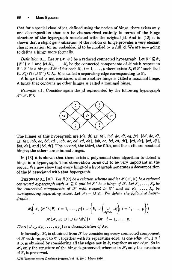
Example 3.1. Consider again the jd represented hy the following hypergrapb Z(“N, E’):

The hinges of this hypergmph are {de, dj, eg, fg), {cd, de, df, eg, fg}, (bd, de, df, eg, fgl, lab, ac, bd, cdl, I& m, bd, cd, de), lab, ac, bd, cd, dfl, Icd, de), (cd, df I, {bd, de], and {bd, df). The second, the third, the fifth, and the sixth are maximal hinges; the others are minimal hinges.

In [13] it is shown that there exists a polynomial time algorithm to detect a hinge in a hypergraph. This observation turns out to be very important in the sequel. We now show that every hinge of a hypergraph generates a decomposition of the jd associated with that hypergraph.

THEOREM 3.1 [lo]. Let R(Q) be a relation dwne and let Z (Jv, 8;) be a reduced connected hypergraph with N C Q and let 8“ be a hinge of 2’. L.et 81, . . , gP be the connected components of Z with respect to Z’ and let E,, , En be corresponding separating edges. Let M; = U Z;. We define the following hypergraphs:

zw, zi u IU WZi”i)l) for i = 1, , p.

Then I Js-0, Jx,, , Jxn) is a decomposition of Jx.

Informally, &“,, is obtained from Z by considering every connected component of &” with respect to Z”, together with its separating edge, as one edge. ;U,, 1 5 i 5 p, is obtained by considering all the edges not in 8; together as one edge. So in Z. only the structure of the hinge is preserved, whereas in 57; only the structure of 8; is preserved.


The Hinge Decomposition Algorithm. We propose to decompose a join-dependency Jn (using the notation introduced above):

(1’) Search for a hinge in X’. If there is more than one hinge, choose one (arbitrary for the time being). If there is no hinge, we cannot decompose Jr by the hinge decomposition algorithm.

(2”) Apply Theorem 3.1 and obtain JxO, , JrJ. (3”) Apply the algorithm recursively on Jzo, , Jx9.

Finally, use Theorem 2.1 to obtain the desired result.

Note that whenever the jd we started with is full, the decomposition we obtain also consists of full jds only.

Example 3.2. Consider the hypergraph X?‘(M, 8) of Example 3.1. From Ex- ample 3.1 we know that {de, df, eg, fg) is a hinge. There is only one connected component with respect to {de, df, eg, fg}, namely, {a6, oc, bd, cdl. de is a separating edge corresponding to it (df 1s another one). The second step of the hinge decomposition algorithm gives us the following hypergraphs:

20 (iv, lab& % eg, fg I ) XI W, lab, UC, cd, bd, defg 1)

Theorem 3.1 asserts that { Jr*, Jx,] is a decomposition of Jx. Since Z?,, does not contain any hinges, Ja, cannot be decomposed any further with the hinge decomposition algorithm. X1, however, contains a hinge, namely, {a6, oc, bd, cd] with cd as a separating edge corresponding to the only connected component (defgJ with respect to this hinge. This gives rise to the hypergraphs:

Both X10 and .Z“,, contain no hinges, so Jx, and Jr,, are not decomposable any further by the hinge decomposition algorithm. [ Jx,,, Jz,,) is a decomposition of Ja,. Finally, Theorem 2.1 states that { J xO, Jx,,, Jx,,] is a decomposition of Jx.

In the following section we give an overview of some properties of the hinge decomposition algorithm, most of which were proved in earlier work.

4. PROPERTIES OF THE HINGE DECOMPOSITION ALGORITHM

In this section we give an overview of some properties of the hinge decomposition algorithm, most of which were shown in earlier work. Some of these properties

90 * Marc Gyssens

are included to illustrate the strength of the hinge decomposition algorithm, whereas others will he needed in Sections 5 and 6, which contain the main results of this paper.

The first result we want to mention characterizes the presence of a hinge and, at the same time, demonstrates the importance of this notion:

THEOREM 4.1 [IO, 121. Let R be a relation scheme and J be a reduced and connected jd. Then the followingproperties are equivalent:

(1”) J is decomposobk; (2’) Z?J contains a hinge; (3”) There exists E E Z., such that gJ\(E) is not a connected subset with respect

to (Ej.

Example 4.1. Clearly, a jd that contains hinges is decomposable (by means of the hinge decomposition algorithm). Theorem 4.1 also claims the converse. This allows to check for decomposability by looking at the hinges. Consider the jd:

ab w bc w cd w de w ef w fg w ga. It can easily be seen that this jd does not contain a hinge, either by a straightforward verification or by using the implication (2”) + (3’) of the previous theorem. Hence the above jd is undecomposahle, which proves what was already claimed in the Introduction and in Example 2.2

In order to phrase some important properties of decompositions generated by the hinge decomposition algorithm? we need to introduce some additional terminology concerning decompositions.

Definition 4.1. Let J be a jd and suppose that I J,, , J.) is a decomposition of J. This decomposition is said to be final if none of the J:, i = 1, . . . , s is decomposable. This decomposition is said to he nonredundant if for each i = 1, , s, ( J1, . . , Jim,, Ji+,, . . , Ja) =#a J;.

Clearly, getting a final and nonredundant decomposition is an important property of a decomposition methodology. We have the following:

THEOREM 4.2 [lo]. Every decomposobk reduced and connected jd can be decomposed with the hinge decomposition algorithm into a final and nonredundant decomposition.

Example 4.2. Consider again the jds and hypergraphs of Example 3.2. We know already that ( Jx., Ja,,, J1;,) is a decomposition of Jz. By Theorem 4.2, this decomposition is also final and nonredundant. The first claim already follows from Theorem 4.1; the second one implies that none of the three jds in the decomposition can be omitted.

Furthermore, it is possible to generate decompositions with the hinge decomposition algorithm in a time that is polynomial in the size of the input:

THEOREM 4.3 [13]. Let R(Q) be o relation scheme with 1 R 1 = m and kt J be (I jd ouer R with k edges. Let n = km. Then it is possible to generate a final decomposition of J with the hinge decomposition algorithm in O(n3) time. ACM nm%aetions on “alnbase systems, “0,. 11, No. 1. March ,986.

Complexity of Join Dependencies 91

Furthermore, a final decomposition obtained with the hinge decomposition algorithm contains at most k - 1 jds.

PROOF. The proof of the first claim in Theorem 4.3 uses characterization (3’) of Theorem 4.1 for the presence of hinge..Since the proof is too long to include in this paper, we refer to [13] for further details. We now show the second part of Theorem 4.3. Let (51, . . , J.) be a decomposition (not necessarily final) obtained after a number of steps of the hinge decomposition algorithm. Let (r be the sum of the numbers of edges of J1, . , J.. Then it can be easily shown by induction on the number of steps needed to obtain the decomposition that

o=k+s-1. (1)

Since each jd in the decomposition contains at least two edges, we have that

Substitution of (2) in (1) yields

CT 2 2s. (2)

In particular, this equation also holds for a final decomposition obtained with the hinge decomposition algorithm. 0

It follows from Theorem 4.3 that an scyclic jd with k edges is equivalent to a set of k - 1 mvds, since the inequality (2) becomes an equality in that case.

Since hinges play a crucial role in the hinge decomposition algorithm, we may expect that there exists a close relationship between the jds of a decomposition obtained with the hinge decomposition algorithm and the “hinge-structure” of the jd that was decomposed. This relationship is expressed in Theorem 4.4, below. In order to prove this theorem, we need some lemmas. The first lemma was proved in [lo].

LEMMA 4.1. Every final decomposition of a jd obtained with the hinge decomposition algorithm can also be obtained by using only maximal hinges. In this way we obtain in each step of the decomposition process exactly two jds of which at least one is decomposable.

Example 4.3. Consider again the decomposition obtained in Example 3.2. We show that this decomposition can also be obtained by using only maximal hinges. We know from Example 3.1 that lab, oc, bd, cd, de} is a maximal hinge of Z. An application of Theorem 3.1 with this hinge gives us also the hypergraphs .Zs and /Ml, but in the opposite order. Furthermore, (ab, ac, bd, cd} is a maximal hinge of .z,. We often represent a decomposition process using only maximal hinges by a binary tree. The decomposition process in this example is represented by

LEMMA 4.2. Let R be (I relation scheme and let J be a jd ouer R. Let Z?’ be a maximal hinge of ZJ. Then ZJ\Z ’ is connected. Let E be a separating edge of $ ’

ACM Transactions on Dstebasc Systems, Vol. 11, No. 1, March 1986.

92 * Marc Gyssans

corresponding to 87.~. Then (gJ\Z?“) U (EJ is also a hinge of Z., and E is o separating edge of this hinge corresponding to every connected component with respect to that hinge. Finally, if JO and 5, are the jds in the decomposition defined by W’ (according to Theorem 3.1), then J, and JO eon be obtained from J by replacing the edges of iZ ’ respectively, (e;\8 ’ ) U (E) by their union.

PROOF. A straightforward verification shows that gJ\8 ’ is connected. (Other- wise, 8’ would not he a maximal hinge.) We show that (Z?J\~‘) U (E) is a hinge of gJ of which E is a separating edge corresponding to every connected component with respect to it. This follows from the fact that each edge not in (~J\Z’) U (E) necessarily belongs to Z? ’ and that E is a separating edge of Z ’ corresponding to ~J\Z’. The remaining part of the lemma follows from a simple look at the hypergraphs in Theorem 3.1. 13

Example 4.4. In Example 4.3 we pointed out that Jx, and Jx. can be obtained from Jn by a decomposition using the maximal hinge (ab, ac, bd, cd, de]. Clearly, de is the only separating edge of this hinge corresponding to (df, eg, fg}, which is connected to (ab, oc, bd, cd, de). A straightforward verification shows that (df, eg, fg, de] is also a hinge and that de is a separating edge of this hinge corresponding to the (only) connected component (ab, oc, bd, cd) with respect to it. Clearly, JzO is obtained from Jx by replacing (ab, oc, bd, cd, de) by its union, whereas Jz-~ is obtained from JX by replacing (df, eg, fg, de) by its union.

LEMMA 4.3. Let R be o relation scheme and J: X, w w Xk o reduced and connected jd over R. Let { J,, , J.) be a final decomposition of J obtained by using hinges. Let, for i = 1, . . , s, J, be the jd Y;, w . w Y;+ Then, for all i = 1, . , s and for ollj = 1, . . , kc, there exists 1 5 to _C k with X,, G Y;j and Yij:,n(U(Y~;l~l~kinndl#jJ)~X~jj.

PROOF. We can assume that the above decomposition is obtain by using maximal hinges only (Lemma 4.1). Let

.I JO.1 50.2 - - - JO,,., - JO,,-, = J.

be a tree representing the decomposition of J into ( J1, . . . , J.) as in Example 4.3. We prove by induction on their depth in the tree that all the jds in that tree satisfy the property of Lemma 4.3.

On depth 0, we have only J itself, and, for J, Lemma 4.3 is trivially satisfied. Suppose now that all jds in the above tree until depth m satisfy the property of Lemma 4.3. Let J’: Y, w w Yp be a jd in this tree on depth m + 1. For notational convenience, we prove that there exists 1 5 t c p with X, c Y, and Y, n (Yz U U Y,) C X,. Let J”: Y; w w Y;, (p’ >p) be the father of J ‘. We distinguish two possible cases:

Case 1. YI is an edge of J”. Without loss of generality we can assume that YI = YI’. By induction there exists 1 5 t I s with X, C Y; and Yi f~ (Y;U...UY,‘,)cX,.Clearly,X,CYI,and

Y~n(Y,U.-.UY,)=Yin(Y;U...UY6,)rX,.

ACM Tmaactions on Datahe System. Yo,. 11, No. 1. March 1986


Case 2. YI is not an edge of J “. Then, according to Lemma 4.2, there exists a hinge of &4r- such that Y, is the union of that hinge. Without loss of generality, let {Y; , , Y; }, q < p ’ be that hinge. Also, this hinge contains a separating edge corresponding to all the connected components with respect to that hinge. We can assume that this separating edge is Y;. Now let X, be as in Case 1. Then

Y,ll(Y2U’.. uY,)=(Y;u... uY,‘)n(Y;+lu.~~uY;.) cy;n(y;+,u...u~;~) c Y; n (y; u u y;,) c x,.

This completes the proof. 0

Example 4.5. We know from Example 3.2 that

J+ &de w df w eg w fg Jz,.: ab w oc w bd w cdefg

Jx,,: obcd w defg

is a decomposition of

Jx: ab w oc w bd w cd w de w df w eg w fg.

The edges of J.v satisfying the conditions of Lemma 4.3 are, as is easily verified, (in the same order as above)

for JxO: de, df, eg and fg;

for JzIO: ob, oc, bd and cd;

for J,v~,: bd (or cd) and de (or df ).

We can now prove the actual theorem.

THEOREM 4.4. Let R be a relation scheme and J: X, w m Xa be II reduced and connected jd over R. Let { J,, . . , J.) be (I final decomposition of J obtained with the hinge decomposition algorithm. Suppose, for i = 1, . , s, that Ji is the jd Yi, m m Yik.. Then there exist 1 5 t,,, . , thi s k such that

- for all j = 1, , k;, P$,L Y;j (and hence all the X, ore different); - IX,,, , X,,) is a nmrml hinge of .ZJc.; - for all j = 1, , k;, Y;j is the union of Xto and all the edges of some connected

components &; with respect to IX,,, . . , X,) for which Xt, is a corresponding separating edge.

PROOF. Choose X,,, , X, as in Lemma 4.3. Then, for 1 I I # m 5 k;, we have that Yti n Y:,,, C X, n X,_: Hence Y, and Yti are disconnected with respect to IX,,, . , X,,). Furthermore, we have that

k;, n (x+, u u x+,) C yil n (x,, u Yi2 u u Yik) c x,, u (Yil n (yi2 u u yai)) L x,,

and mutah mutan& for the other indices,

Yij n (x,, u u Xt%) G X,. ACM Transactions on Database Systems, Vol. 11, NO. 1, March 1986.

94 * Marc Gyssens

Hence IX,,, . . , Xt*} is a hinge satisfying the first and third conditions of Theorem 4.4. It remains to show that this hinge is minimal. Suppose this would not be the case. Then, after a possible renaming of indices, let IX,,, . . , Xt,), p < k; be a maximal hinge of IX,,, , X+1 with X,, as separating edge corresponding to (Xti,+,), . . . , Xt*l. Then

(Y;1 u ... u Y,) n (Y;cp+,, u ... u Y*J =U~Y~nY,,;l~l~p,p+lcm_ckjj c u (X, r-l x,; 1 I I 5 p, p + 1 5 m 5 kc{ = (Xtt, u “. u xt*, n (xtt(,,, u ‘.’ u x**, c xq, L Yi,.

Consequently, ( Yi,, . , Y,) is a hinge of Z+ in contradiction with our decomposition being final (cf. Theorem 4.2). So IX,,, . . , Xtyj is indeed a minimal hinge of ZJ. 0

We conclude this section with an illustration of the previous theorem.

Example 4.6. Consider again the hypergraph .? of Example 3.1 and the decomposition of Jx obtained in Example 3.2. Minimal hinges of .%?’ satisfying Theorem 4.4 for the various jds of this decomposition are

- for 20: we, df, eg, fgl; - for Z,o: (ab, (IL‘, bd, cd 1; - for .?‘,I: {cd, de!.

For the last jd, we could also have taken {cd, dj], (bd, de{ or (bd, df).

5. THE COMPLEXITY OF INTEGRITY CHECKING

An important reason for replacing a join dependency by a decomposition is making integrity checking less time consuming. Indeed, performing a join requires a time exponential in the number of edges that are to he joined. It therefore is important to minimize the size of the largest jd to be taken into account. This leads us to the definition of the degree of cyclicity of a jd, which is stated in Definition 5.2. (A very similar definition has also been stated independently in [la].) We then characterize the degree of cyclicity of a jd in terms of the jd itself and show that our decomposition methodology generates decompositions that satisfy the above minimality criterion. Finally, we define n-cyclic jds as jds whose degree of cyclicity is at most n and we show that for a fixed value of n, integrity checking can be performed in polynomial time, provided only n-cyclic jds are considered.

We first establish some notations.

Definition 5.1. Let R be a relation scheme and J be a reduced and connected jd over R. Then

- DEC( J) is the set of all decompositions of J augmented with J itself; - MINHIN( J) is the set of all minimal hinges of &;; and - 1 J I is the number of edges of J. ACM Transactions on Database Systems, Vol. 11, No. 1, March 19ss.


Definition 5.2. Let R be a relation scheme and J be a reduced and connected jd over R. We define the degree of cyclicity of J, denoted dgr( J), as

dgr( J) = min(max( 1 J’ 1, J’ E 81, / E DEC( J)).

In words, the degree of cyclicity of a jd is the minimum over DEC( J) of the number of edges of the largest jd in an element of DEC( J). From the definition of “decomposition of a jd” (Definition 2.10), it immediately follows:

LEMMA 5.1. Let R be a relation scheme and J a jd ooer R. Then dgr( J) c 1 J I. Furthermore, dgr( J) = 1 J 1 if and only if J is undecomposable.

Observe that a (nontrivial) jd is acyclic if and only if its degree of cyclicity equals 2. Indeed, a jd is acyclic if and only if it is equivalent with a set of multivalued dependencies. Obviously, it is impossible to find a “better” decomposition.

Example 5.1. Consider the jd ab w bc w cd w de w ejw fg w go. In Example 4.1 we proved that this jd is undecomposable. Hence its degree of cyclicity equals 7. In particular, this jd is cyclic.

Now consider again the jd JX of Example 3.1. Using one of the many charac- terizations for acyclicity (see, e.g., [2, 3, 8, 9]), it can be shown that Jr is cyclic (we prove this in Example 5.5). Taking into account the above observation, it follows that the degree of cyclicity of JX is at least 3. Since the largest jd in the decomposition of Jr constructed in Example 3.2 has size 4, it follows that dgr( Jz) is at most 4. Later on, we shall see how we can calculate the precise degree of cyclicity of a jd.

Although Definition 5.2 seems a very natural way to define the complexity of a jd, it does not provide an efficient way to calculate the degree of cyclicity of a jd, as was pointed out in the previous example. Therefore, we are now going to show that the degree of cyclicity of a decomposable jd equals the size of the largest minimal hinge of its associated hypergraph. Hence we characterize the notion “degree of cyclicity of a jd” in terms of the jd itself.

We first prove that the degree of cyclicity of a decomposable jd is at least the size of the largest minimal hinge of its associated hypergraph. We therefore need some lemmas.

We first show that equivalence of jds is “inherited” if we “restrict” each jd to a subset of the set of attributes that is involved. We therefore define the “trace” of a jd.

Definition 5.3. Let R(O) be a relation scheme and let J: X, w w X, be a jd over R and let X c R. The trace of J with respect to X, denoted trx( J), is the reductionofX1nXW wX~~X.

Example 5.2. Consider again the jd Jn of Example 3.1. Let X = &de. Then trx( Ja) = ab w ac w bd w cd W de.

LEMMA 5.2. Let R be a relation scheme and let J be a reduced and connected jd ouer R. Suppose that 8’ = (E,, . . , E,J is a hinge of;uJ. Then tr,a,( J) = El w

w E,. ACM Tmmaetions on Datahe System, Vol. 11. No. 1, March 1486.

96 * Marc Gyssens

PROOF. Let E be an arbitrary edge of J not in Z?‘. Since, by definition, there exists 1 _c ; _c 1 such that E n (U 6? ’ ) G Ej, Lemma 5.2 follows.

Example 5.3. Consider again the jd Jx of Example 3.1. In that example we saw that (ab, oc, bd, cd, de{ is a hinge Z’. From Example 5.2 it follows that tra( Jx) = ab W oc w bd W cd w de, in accordance with Lemma 5.2. Note that the condition in Lemma 5.2 that g’ is a hinge cannot be arbitrarily removed (though it can be weakened). Indeed, consider the set (ab, ac, cd, de]. This set is not a hinge of &“, but has the same set of nodes as (ab, ac, bd, cd, de}. Hence tr~(J,)=abwacwbdwcdwde#abwnewcdwde.

LEMMA 5.3. Let R(O) be a relation scheme and let J, 5,, , J. be ja!s ouer R andsrrpposeJo(J1,...,J,}.LetX~R.Thentrx(J)~~Itr,(J*),...,tr,(J,)}.

PROOV. The proof uses the chase technique [14]. Consider the implication “t”. Consider tableaux for J and for trx( J). Each time a jd Ji, 1 5 i 5 s is applied to the tableau for J, we can apply trx( JA in a similar way to the tableau for trx( J). Since the chase for [ J,, . , J,) =+ J is successful, it follows that the constructed chase for {trx( JI), . . , trx( J.)) =+ trx( J) is successful too. The implication “q” can be shown in the same way. 0

Example 5.4. Consider again the jd Jx of Example 3.1 and its decomposition { JxO, Jx,,, JK1lJ constructed in Example 3.2. Let X = abdeg. Then

trx(Jx)= abwbdwdeweg; trx( Ja,) = abde w eg; trx( J,,,) = ab w bd W deg; trx( Jx,,, = abd w deg.

According to Lemma 5.3, we have that ab w bd w de w eg w {abd w de w eg, ab w bd w deg, nbd w deg]. Note that the right-hand side of this equivalence is neither final nor nonredundant.

We can now prove

LEMMA 5.4. Let R be a relation scheme and let J, J1, , J. be jds ouer R with Jreducedandconnected.SupposeJo(J,,...,J,).~t~”=~E,,...,E,Jbea minimal hinge of &;. Then there exists 1 5 i 5 s with 1 J; 1 2 18 ’ I.

PROOF. Let J’ be El w w & From Lemma 5.2 and Lemma 5.3 we know that J’ * ltrVg. ( J,), . , tr,g, ( J,)}. Since .YJ, does not contain hinges (because Z? ’ is minimal), it follows from Theorem 4.1 that J ’ is ondecomposable. Hence thereexists1~i~swithItrUg..(Ji)I~IJ’I.Clearly,IJ’)=I~‘IandIJ;I 2 I tr,,s, ( J;) I, from which the desired inequality follows. 0

As an immediate corollary of Lemma 5.4, we obtain

COROLLARY 5.1. Let R be a relation scheme and let J be a decomposable reduced and connected jd ouer R. Then dgr( J) 2 maxi I g’ I, 8” E MINHIN( J)).

Example 5.5. Consider again the jd J, of Example 3.1. From Example 3.1 it follows that the size of the largest minimal hinge of Jx equals 4. Hence, by Corollary 5.1, dgr( J) > 4. In particular, this result proves that Ja is cyclic. Since we already know (Example 5.1) that dgr( J) 5 4, it follows that dgr( J) = 4. ACM Transactions on Database Systems, Vol. 1,. No. 1, March 1986.


To prove that the inequality in Corollary 5.1 is actually an equality, it suffices to construct for e given decomposable jd a decomposition of which the largest element contains at most as many edges as there are edges in the largest minimal hinge of the hypergraph associated with the given jd. It turns out that the decompositions obtained with the hinge decomposition algorithm satisfy this criterion:

LEMMA 5.5. Let R be a relation scheme and let J be a decomposable reduced and connected jd out-r R. Then dgr( J) 5 max( 1 Z ’ I, i? ’ E MINHIN( J) ).

PROOF. According to Theorem 4.4, the number of edges of a final decomposition of a given decomposable jd obtained with the hinge decomposition algorithm equals the number of edges of some minimal hinge of the original jd. The statement of the lemma immediately follows from this observation. 0

If we combine Corollary 5.1, Lemma 5.5, and Theorem 4.3, we immediately get:

THEOREM 5.1. Let R be a relation scheme and let J be a decomposable reduced and connected jd wer R. Then dgr( J) = maxi 1 Z?’ I, ?7’ E MINHIN( J) ). Furthermore, for each decomposition f of J obtained by using hinges we have that dgr( J = max( ) J’ ) ; J ’ E .f ). Hence each decomposition obtained by our method minimizes the number of edges of its largest component.

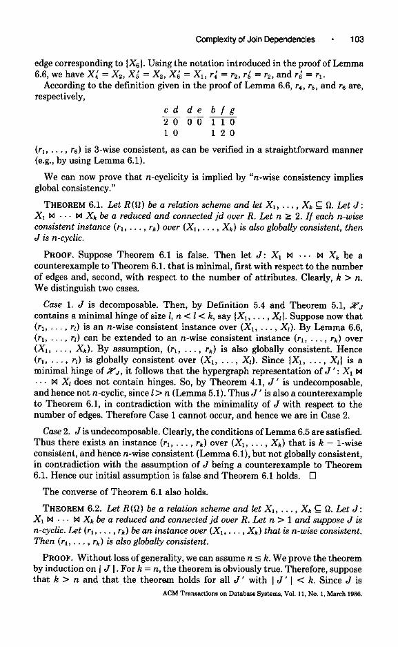
Example 5.6. We already showed for the jd J.v of Example 3.1 that dgr( Jx) = 4. We therefore look at another example. Consider the jd J ’ : ab w ac w bd w cd w ce w dj w ef. This jd can be represented by the hypergraph:

The above hypergraph contains two hinges, (ab, ac, bd, cd) and (cd, ce, df, ef), which are both minimal and maximal. Hence dgr( J ’ ) = 4. Note that this result is obtained without looking at decompositions of J’.

We now use the degree of cyclicity as a tool to classify join dependencies according to their complexity.

Definition 5.4. Let R be a relation scheme and let J be a reduced and connected jd over R. Let n be a positive integer. J is said to be n-cyclic if its degree of cyclicity is at most n.

In this way we obtain e hierarchical classification of join dependencies. Ac- cording to a previous remark, 2-cyclicity is the same es acyclicity. It is well known [2, 3, 6, 91 that integrity checking for acyclic jds can be performed in polynomial time. We now extend this result.

THEOREM 5.2. Let n > 1 be a fixed integer. Let R(O) be a relation scheme and let J be an n-cyclic reduced and connected jd ouer R with k edges. Let m be the number of attributes in Cl. Then checking an instance r ouer R for integrity can be done in a time that is polynomial in m, k, and 1, where 1= ) r )

ACM Transections on Databsse Sya+.ems. “al. 11. No. 1, March 19%.

98 . Marc Gyssens

PROOF. By Theorem 4.3, we can obtain a decomposition of J with the hinge decomposition algorithm on O(k3m3) time. Also by Theorem 4.3, this decomposition consists of at most k - 1 jds. By Theorem 5.1, each of these jds has at most n edges. Hence checking whether such a jd holds can be done in O(l”+‘m) time, as can be shown by straightforward calculation. This means that, using the decomposition, checking whether J holds can be done in O(k3m3 + kml”+‘) time. [3

Hence integrity checking can be done in polynomial time provided only n-cyclic jds are considered for a fixed value of n.

6. THE COMPLEXITY OF CONSISTENCY CHECKING

Instead of using a jd to check a relation instance for consistency after each update, we could also decompose the relation scheme according to the jd, and thus work with smaller relations. If this approach is followed-which is usually the case-the problem of integrity checking is eliminated, since the join of the various “subrelations” by definition satisfies the jd. Nevertheless, we have to make sure that all our subrelations are the projections of a common relation instance over the original relation scheme. In other words, we may not lose tuples by first making the join of all the subrelations and then projecting back onto the edges of the jd. So we have to check our decomposed database for consistency after each update of a subrelation.

A very important advantage of a jd describing the structure of a decomposed database being acyclic is that checking a database instance for consistency can be performed in polynomial time, because acyclicity is equivalent with “pair-wise consistency implies global consistency.” Pair-wise consistency means that every two subrelations are the projections of a common relation instance, and this property can easily be verified in polynomial time. In this section we generalize this result by proving that n-cyclicity is equivalent with “n-wise consistency implies global consistency.” Thus checking for (global) consistency remains solvable in polynomial time if we restrict ourselves to n-cyclic jds for a fixed value of n.

We first recall some well-known basic facts about consistency and introduce the necessary notation. We then prove the two lemmas we need to show that “n-wise consistency implies global consistency” is a sufficient condition for n-cyclicity. We then prove that it is also a necessary condition. Finally, we show that checking for (global) consistency can be performed in polynomial time, provided we restrict ourselves to n-cyclic jds for a fixed value of n.

Definition 6.1. Let R(Q) be a relation scheme and let X,, . , Xa C Q. Let (rl, , Q) be an instance over (X1, . . , Xa). Let n be a positive integer.

- If n 5 k, then (rl, , rh) is called n-wise consistent if for each subsequence il, , in of 1, , k there exists an instance r over X, U U Xi” satisfying 7r+(r) = ri, for all t = 1, . , n.

- (rl, , ra) is called globally consistent if it is k-wise consistent. - If n > k, then (r, , . , rk) is called n-wise consistent if it is globally consistent.

We can now make some straightforward observations:

LEMMA 6.1. Let R(n) be (I relation scheme and kt X,, .., X, C n. Let (r,, , n,) be an instance ouer (Xl, . , X,). Let n be a positive integer. Let

ACM Transactions on Database Systems, Vol. 11, No. 1, March 1986.


m 5 n. If (r,, , rk) is n-wise consi.stent, then it is also m-wise consistent. Suppose n 5 k. Then (r,, . . , ra) is n-wise consistent if and only if for each subsequence i,, . . , i,ofl,..., kandforallt=l,..., II we kaue that Q$(“, w w Ti”) = ri,.

LEMMA 6.2. Let R(Q) be a relation scheme and let X1, , X, C 0, k > 2. Let 1 < 1 < k. (rl, , rh) is a globally consistent instance ouer (XI, , XJ if and only if (r,, , r,) is globally consistent ouer (XI, . , X,) and (rI w w r~, r~+,,

, ra) is glob&y consistent ouer (Ufx, Xi, X,+1, , Xd.

The last observation concerning Definition 6.1 we want to make here deals with Z-wise consistency, which is usually called pair-wise consistency. It can be easily seen that pair-wise consistency can be checked in the following way:

LEMMA 6.3. LA R be a relation scheme and let XI, , Xa C Cl. Let (rl, . , rk) be an instance over (X,, , X,). (r,, , Q,) is pair-wise con.sistent if

Vl 5 i #j 5 k: rxjnxj(r.) = rxinxi(rj),

We illustrate the notion of consistency with the following example:

Example 6.1. Let R(a) be a relation scheme and let Q = abc. Let (r,, rz, r3) be the following instance over (ab, be, ac):

ab bc ac 11 13 43 41 52 ‘12 15

Clearly, the projections of r, and r2 onto b = ab n bc both equal

b 1 5

The projections of rz and r3 onto c = bc fl ac both equal

and the projections of r, and r3 onto a = ob n ac both equal

a 1 4

Hence, by Lemma 6.3, (rl, r2, ra) is pair-wise consistent. Calculating rl w rz W r3 gives

abc 413 152

Clearly, rd(rl W rz w rJ # r,. Thus, by Lemma 6.1, (r,, rz, r3) is not globally consistent.

100 * Marc Gyssens

We are now going to prove that a n-cyclicity is implied by “n-wise consistency implies global consistency.” We therefore need two technical lemmas (Lemmas 6.5 and 6.6). In view of the assumptions we made in Section 2, we can assume without loss of generality that all the domains involved contain the set of all nonnegative integers and all pairs of nonnegative integers. We introduce the following notation, which is needed in Lemma 6.5.

Definition 6.2. Let R(R) be a relation scheme and let XC R. Let (Y,, , Yl) be a partition of X and let i,, . , i, be nonnegative integers or pairs of nonnegative integers. Then iI,,> il, denotes the tuple over X that associates the value k with each attribute of Yj for each j = 1, . . . , 1.

Example 6.2. Let 0 = X = abcdefg. Let Y, = abc, Y2 = de, and Y3 = fg. Then Oy,2y,(2, 3h, denotes the tuple

abcde f g 0 0 0 2 2 (2, 3) (2, 3) .

Using this notation we can easily calculate the projection of a tuple:

LEMMA 6.4. Let R(a) be a relation scheme and let Z L XC a. Let {Y,, . , Y,) be a partition ofX and let i,, . , i, be nonnegative integers or pairs of nonnegatiue integers. LA

ilyl i,

be a tupk over X. Then the projection of this tupk onto Z is

G,nz ... i,“@.

The proofs of both Lemma 6.5 and Lemma 6.6 are notationally rather involved. Therefore, we give here only the main constructions of these proofs. The reader can find further details in the Appendix. The constructions made in these lemmas are subsequently illustrated by examples (Examples 6.3 and 6.4). We advise the reader to consult these examples while examining the lemmas and their proofs.

LEMMA 6.5. Let R(0) be a relation scheme and kt X;, . . , X* C 0, k > 2. Let X = U?=, XC. Suppose J : Xl w . w X, is a reduced and connected undecomposabk jd without attributes occurring in only one edge. Define the instance (rl, , ra) OLJW (X,, , X,) a.3 folhJs:

?I = lox,1 U 10x,nxjk jh,\q; 2 5 j Z t 5 kj; c = 10~,n~,n~,t~~,n~j,\~,(t, i )x,+ 2 5 i Z t 5 kl, i + 1.

Then (r,, ra) is k - l-wise consistent, but not globally consistent.

PROOF. To show that (rl, , rJ is k - l-wise consistent, it suffices to construct relation instances r, over X, 1 = 1, . . , k satisfying r; = nxj(r’) for 1# i. Therefore, define

r’ = 10x,nx.tx.\x,(t, j)x\+; 2 5 j # t 5 k); I I r’ = ~ox,lx\x,l u rl, 1 # 1.

A straightforward verification using Lemma 6.4 shows that for 1 5 i # 1~ k we have it indeed that rx,(r’) = r:. Thus (r,, , ra) is k - l-wise consistent. The ACM Transactions on Database Systems, Vol. I,, No. 1, March ,986.

Complexity of Join Dependencies . 101

proof that (r,. , ra) is not k-wise (globally) consistent can be found in the Appendix. 0

Example 6.3. Let Q = X = abed. Let X, = ab, X, = bc, X, = cd, and X, = da. Then rL, r2, r3, and r, are, respectively,

b i 0

b 0 i ( i = 2. t = 3)

(3.2) 0 (j=2,t=3) 0 4 i) = 21 t = 4j (4,2) 0 (j=2,t=4) (2,3) 2 (j=3,t=2) (2,3) (2,3) (j=3,t=2) (4,3) 4 (j=3,t=4) (4, 3) (4, 3) (j = 3, t = 4) (2, 4) (2, 4) (j = 4, t = 2)

0 (2,4) (j=4,t=2) (3,4) (3,4) (j=4,t=3) 0 (3, 4) (j = 4, t = 3)

i (3d2) (j = 2, t = 3) (3f2) (3p2) (j = 2, t = 3) (4, 2) (i = 2, t = 4) (4, 2) (4, 2) (j = 2, t = 4)

2 (J=&t=2) 2 (2, 3) (j = 3, t = 2) 4 (j=3 t=4)

(2:4) 2 (j=4:t=2) (4, 3) (j = 3, t = 4)

0 (j = 4, t = 2) (3,4) 3 (j=4,t=3) 3 0 (j=4,t=3)

The relation r’ in this example is

b (3% 0 i (3f2) (j = 2 t = 3) (4, 2) 0 4 (4, 2) (j = 2: t = 4) (2, 3) (2, 3) 2 2 (j = 3, t = 2) (4, 3) (4, 3) 4 4 (j = 3, t = 4)

0 (2, 4) (2, 4) 2 (j = 4, t = 2) 0 (3, 4) (3, 4) 3 (j = 4, t = 3)

r* equals r’ augmented with the tuple

a b c d 0 0 2 2’

r3 equals Y’ augmented with

a b c d 0 0 3 3’

and r’ equals r’ augmented with

a b c d 0 0 4 4

It is a straightforward verification that for i, 1 = 1, . . . , 4, i # I it holds that r.rj(r’) = 7;. Hence (rl, r2, r3, r4) is 3-wise consistent. It is also easy to verify that rl W r~ W r3 W rr = r’. Since OX, B I,, TX,@, w r2 w r3 w r,) # r,. Hence (r,, rz, r3, r,) is not globally consistent, in accordance with Lemma 6.5.

102 * Marc Gyssens

LEMMA 6.6. Let R(R) be a relation scheme and let Xl, ., Xh C R. Suppose that J: X, w w X, is a reduced and connected jd ouer R and let g’ = ~X,,...,X1},1<kbeahingeof~~.LetnsIandsuppose(r,,...,r~)isann- wise consistent instance ouer (X,, , Xl). Then (rl, , r,) can be extended to an n-wise con.sistent instance (r,, . , rk) ouer (X,, . , Xd.

PROOF. Choose for each connected component of .ZJ with respect to SY”’ a fixed corresponding separating edge of SY ‘. For 1+ 1 5 j I k, we denote with X/ the separating edge corresponding to the connected component to which Xj belongs. Suppose 1+ 1 5 j 5 k. Let r; he the instance in {r,, , rl] defined over X; and let rj be the instance over Xj defined as

rj = (tl3t’ E r;: t[xj n x;] = t’[Xj n Xi] & va E x,\x;: t(a) = 0).

Then (r,, . . , rk) is an n-wise consistent instance of (XI, , Xh). (Details of the proof can be found in the Appendix. 0

The constructions made in the proof of the previous lemma are illustrated in Example 6.4, below.

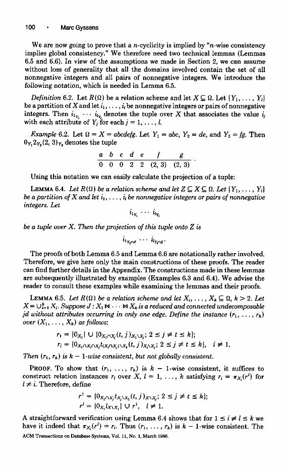
Example 6.4. Let XI w w X6 be represented by the following hypergraph z:

Clearly, {XI, X,, X3} is a hinge of Z. Let (rl, ~2, ~5) be the following over (X,, X2, X3):

abf bc ac 111 12 12 212 11 21 112 11

Clearly, (r,, r2, ~3) is (3-wise) consistent because r,, rz, and r3 are the projections onto XI, X,, and X,, respectively, of, for instance,

a b c f 1 1 2 1 2 1 1 2 1 1 1 1 1 1 1 2

We are now going to extend (r,. r~, r3) to a 3-wise consistent instance (rl, . . , r6) over (X,, , X,). We first have to assign fixed separating edges to the connected components of Z with respect to 8”. Therefore, we choose X2 as a separating edge corresponding to IX,, X51. Clearly, X, is the only separating


edge corresponding to IX,). Using the notation introduced in the proof of Lemma 6.6, we have X; = X2, X; = X,, X; = X,, r; = 1.2, r; = rz, and r; = r,.

According to the definition given in the proof of Lemma 6.6, r,, q,, and rs ere, respectively,

cd de bfg 20 00 110 10 120

(rl, , rs) is 3.wise consistent, as can be verified in a straightforward manner (e.g., by using Lemma 6.1).

We can now prove that n-cyclicity is implied by “n-wise consistency implies global consistency.”

THEOREM 6.1. Let R(O) be a relation scheme and let X,, . , Xa C R. Let J: X1 w w X, be a reduced and connected jd over R. Let n 2 2. If each n-wise con.swtent in.stance (r,, . , ra) over (X,, , X,) is ah globally consistent, then J is n-cyclic.

PROOF. Suppose Theorem 6.1 is false. Then let J: X, w w X, be a counterexample to Theorem 6.1. that is minimal, first with respect to the number of edges and, second, with respect to the number of attributes. Clearly, k > n. We distinguish two cases.

Case 1. J is decomposable. Then, by Definition 5.4 and Theorem 5.1, Z., contains a minimal hinge of size 1, n < 1< k, say {XI, . , X(1. Suppose now that (rI, , r,) is an n-wise consistent instance over (X,, , X,). By Lemma 6.6, (rl, . , R) can be extended to an n-wise consistent instance (r,, , ra) over (X,, , X,). By assumption, (rI, , rk) is also globally consistent. Hence (r,. , rl) is globally consistent over (X,, . . , Xi). Since {XI, , X,1 is a minimal hinge of ZJ, it follows that the hypergraph representation of J ’ : X, w

w XI does not contain hinges. So, by Theorem 4.1, J’ is undecomposable, and hence not n-cyclic, since 1> n (Lemma 5.1). Thus J’ is also a counterexample to Theorem 6.1, in contradiction with the minimality of J with respect to the number of edges. Therefore Case 1 cannot occur, and hence we ere in Case 2.

Case 2. Jis undecomposable. Clearly, the conditions of Lemma 6.5 are satisfied. Thus there exists an instance (rl, , rh) over (XI, , X,) that is k - l-wise consistent, and hence n-wise consistent (Lemma 6.1), but not globally consistent, in contradiction with the assumption of J being a counterexample to Theorem 6.1. Hence our initial assumption is false and Theorem 6.1 holds. 0

The converse of Theorem 6.1 also holds.

THEOREM 6.2. Let R(O) be a relation scheme and let X,, , X, C n. Let J: X1 w w Xa be a reduced and connected jd over R. Let n > 1 and suppose J is n-cyclic. Let (r,, , r*) be an instance ouer (XI,. , X*) that i.9 n-wise consistent. Then (r,, . , ra) is also globally consistent.

PROOF. Without loss of generality, we can assume n c k. We prove the theorem by induction on ( J I. Fork = n, the theorem is obviously true. Therefore, suppose that k > n and that the theorem holds for all J’ with 1 J’ 1 < k. Since J is

ACM Tmnsactions on Database System, Vol. 11, NO. 1, March 1sss.

104 * Marc Gyssens

n-cyclic, there exists a minimal hinge of &4r, say (X1, , Xl1 with 15 n. By the induction hypothesis,

? = r, w w r,

sat&es I = ri for all L = 1, , 1. We stdl have to show that (r, rr+l, , d is n-wise consistent over (Ut=, Xi, XL+,, . . . , X,). Since (Uf=, XC) W Xl+, W w X, is clearly also n-cyclic, the induction hypothesis and Lemma 6.2 will then yield the desired result. Therefore, choose for each connected component of ir; with respect to IX,, , Xl) a fixed corresponding separating edge and let, for 1 5 i 5 I, 9; he the set of all the edges of connected components for which Xi is chosen as corresponding separating edge. Now take n instances out of i, R+I, . . . . Q. We may assume that i is among those n instances, since in the other case the proof of their being consistent is trivial. For the sake of simplicity of notation, suppose that those n mstances are r, r~+,, , ri+,-,. Again, without loss of generality, (hy rearranging indices) we can assume that 9, # 9 and that 91 = I-%+*, t, X,) with 1+ 15 t I 1+ n - 1. Define

s = r,+, w t w rt.

Clearly, because of the assumptions, xxi(s) = rj for all j = 1, . , t. Note that by Lemma 6.2 (r, , s) is a pair-wise consistent instance over

since (Q, rl+,, . . . , rt) is globally consistent over (X,, X,,,, . . . , X,) by the n-wise consistency of (r,. , rh) over (XI, . . , X,). Now

*c~.,x.r”,&.,xj~m = %“,L&x,,(~) (hy definition of 9,)

= ~,“,ti&&,,h,(a = ~X,“W~+,&,h)

= ~x~“,u!!.lxJd (by (*) and Lemma 6.3)

= wJ,ntL$~*,xj,(s) (by definition of F1).

Hence by Lemma 6.3,

1

?r&&(i w s) = i

“ti*,x,(i w s) = s

and hence by Lemma 6.2,

s,(i w s) = ri for i = 1, . ( t.

Note that i w s = rl w w rt. By continuing the above argument we eventually get

l

q&&.(i w r,+, w w Ii+,-,) = i sxc(rl W W rr+.-,) = r; for i = 1, . , 1 + n - 1

This completes the proof. 0 ACM Tmnenctiona on Database Systems, Vol. 11. No. 1. March ,986.


Theorems 6.1 and 6.2 can be summarized as follows.

THEOREM 6.3. LA R(0) be a relation scheme and let X,, , X, C 0. Let J: XI w w X, be a reduced and connected jd ouer R. Let n 2 2. Then J is n-cyclic ijand only if each n-wise con&tent instance (r~, . , rk) ouer (XI, . . , XA) is also globally consistent.

Theorem 6.3 generalizes the well-known result that acyclicity is equivalent with “pair-wise consistency implies global consistency.” From Theorem 6.3 we can derive an important corollary, as follows:

COROLLARY 6.1. Let n > 1 be a fixed integer ati kt R(R) be a relation scheme and kt X,, , Xa L R. LA J : X, w w X, be an n-cyclic reduced and connected jd ouer R. Let m be the number of attributes in a. Then checking an instance (r,, , ra) ouer (X,, , X,) for global corwistency can be done in a time that is polynomialinm,k,and1,where1=max~)r~~;i=1,...,kJ.

PROOF. Because of J being n-cyclic, it suffices to check (Q, , rk) for n-wise consistency. Let rf,, , r,” be n relations out of rl, , rh. Making the join r+ w w rI, can be done in O(l”m) time. Checking rti & Q$~~ w w rtn) can be done in O(l”+’ m) time. Hence, to check this for all i = 1, , n, we need O(1”” m) time, since n is fixed. Since we can choose n relations out of k in (2) 5 k” ways, we obtain a total time complexity of O(mk”l”+‘). 0

Corollary 6.1 says that checking for global consistency remains polynomial if we restrict the complexity of the jds we allow, but not necessarily to acyclicity.

APPENDIX

Here we include the details of the proofs of the technical Lemmas 6.5 and 6.6. For the convenience of the reader, we also recall the statements of the lemmas.

LEMMA 6.5. Let R(a) be a relation scheme and kt X,, ) X* L 0, k > 2. Let X = L&, X,. Suppose J : X, w w X* is D reduced and connected undecomposabk jd without attributes occurring in only one edge. Define the instance (r,, . , r*) ouer (Xl, , Xa) a.3 follows:

r, = (OX,] U {O,,,+(t, j)x,\x,; 2 5 j # t 5 kl;

r; = 10x,nx.n~it(x.nxj)\x,(t, i )x,w,; 2 5 j Z t I kl, i # 1.

Then (r,, . , ra) is k - l-wise consistent, but not globally consistent.

PROOF. Recall that the constructions made in this lemma are illustrated in Example 6.3. We already showed that (Q, , Q) is k - l-wise consistent. Hence it suffices here to show that they are not k-wise consistent.

Suppose that (r,, , Q+) is globally consistent. Then there exists T E r, w w rk with 7[X,] = OX, and r[XJ E ri for i # 1. Therefore we can denote 7[X,]

for i # 1 as

106 * Marc Gyssens

We distinguish two possible cases:

Case 1. There exists i # 1 with Xi # Xjj. Suppose 2 c r # ji 5 k. Since J is undecomposable, we have, by Theorem 4.1, that ZJ\(Xj:) is connected with respect to {X,1. Hence there exists a sequence X,,, . , X, with

X”, = x;; x, = x,;

Consider

+c8J = 0, ,nx,n~trz,cx,nx,,\x, (t ‘) u,, Ju, AG,,\&,.

Since X, I-I (X,,\X,) # p, it follows that necessarily (t*, j,) = (t;, jJ and

TIX,] = Ox,nx,nx,~t.(x,\xj~)\x,(t,, ii)x,\+

since this is the only tuple in r, containing the value (t., ji). By continuing this argument we eventually obtain

+Cl = Ox,nx,nxi,ti(x,nx,,\x,(ti. iLip,, and this holds for 2 5 r # ji 5 k. Since r[XI] = Ox,, it follows that

va E x,: 7(a) = 0; Va E U ((X, fl Xjs)\X, 12 5 r # ji 5 kj: T(Q) = t;;

Va E U (X,\Xji 12 5 r # j; 5 kj: ~(a) = (ti, ii).

By assumption (no attributes occurring in only one edge), we have that u IX,; 15 r # ji 5 kJ = X. Hence X\XI = U (X,; 2 5 r # j; c k}\Xl. This gives us that

((u (X,; 2 5 r # J; 5 k)) n X,)\X, = Xj;\X,.

Since X, U (X,\X,) U (X\(X, U Xjt)) = X, it follows that

7 = Ox,4x,Gx,\x, (ti, ji)ncx,ux~i~,

and hence X\(X, U Xji) = (U IX,; 2 5 r # j; s k))\Xj;. Thus

X1 = X1 n (U IX,; 2 I r 5 k}) C (X, n X,) u (X, n (u IX,; 2 5 r f j; 5 kl))

C X, u (Xl n ((u {X,; 2 5 r # j; 5 k))\Xji))

= x, u (x, n (x\(x, u x,)))

= x,.

This is clearly in contradiction with our assumption of J being reduced. Hence we are in the second case.

Case 2. For all 2 5 i c k, Xi = X,. This means that for i # 1 we have

d-G1 = %“xhx,,x,.


Since, by Theorem 4.1, 1x2, , X+.1 is connected with respect to {X1), we can deduce as in Case 1 that for 2 I i, j c k we have that ti = tj. Let us call this value t. Since U IX;; i # 1) = X, we have that

This implies 7 = ox,tx\x,.

4Gl = ox,“x,b,\x,. This tuple, however, is not in rf. Hence our assumption is false and (rl, . . . , rk) is not globally consistent. This completes the proof. 0

LEMMA 6.6. Let R(a) be a relation scheme and let X,, . . . . X, C a. Suppose that J: X1 w w X, is a reduced and connected jd ouer R and let 8’ 1x1, . ..) X,1, 1 < k be a hinge of 2~. Let n 5 1 and suppose (r,, , r,) is an n-wise consistent instance ouer (X,, . . , X,). Then (rl, , r,) can be extended to an n-wise consistent instance (r,, , rk) over (XI, . . , Xa).

PROOF. We recall that we chose for each connected component of iy, with respect to Z? ’ a fixed corresponding separating edge of +? ‘. For 1+ 1 I j 5 k, we denoted with Xi the separating edge corresponding to the connected component to which Xj belongs and with r; the instance in (rl, . . , riJ defined over X/ Finally, for 1+ 1 5 j 5 k, the instance rj over Xj was defined as

r, = ItI 3t’ E r;: t[x, n xi] = tf[xj n x:1 & VQ E x,1x;: t(a) = 0). It remains to prove that (r,, . , r.J is indeed an n-wise consistent instance over (Xl,. , Xd.

First, let us put for 1 5 j 5 I:

rj = rj.

Suppose rt,, , rts are n instances out of r,, , ra. We show that r+(rt, w w rtJ = r+ for 1 5 j 5 n. It suffices to show the inclusion from the right to the left, because the other one is obvious. We distinguish two cases.

Case 1. 1 5 tj I 1. Let T ’ E rti. Because of the n-wise consistency of r,. , r,, there exists i E ri w w r; with i[X,] = 7 ‘. Now define 7 over U;=, X, by

Let 1 5 j’ 5 n. If 1 5 tj, 5 1, clearly, r[X+] = i[X,.] E r+. Suppose now that I + 1 5 tj, 5 k. Then T[X+ n X4] = i[X,. n X4], and for all c E X,]\X4, 7(o) = 0. Hence, by definition, T[X,] E rt;. Thus, for all 1 5 j’ 5 n, we have that r[X,] E rl;, and hence 7 E rt, w w rln. In particular, r[X,] = 7’. This completes the proof in Case 1.

Case 2. 1 + 1 5 tj c k. Let 7’ E rt,. Then there exists T” E r{ such that - ’ [X, n X4] = T y [X, n Xl:]. and for all a E X,\X;, T ‘(a) = 0. As in Case 1,

ACM tinsanions on Database systems. Vol. 11, No. 1, Malrh ,986.

108 - Marc Gyssens

there exists i E r; w w r: with ?[X&] = 7”. The construction of T and the rest of the proof for Case 2 goes as in Case 1. 0

ACKNOWLEDGMENTS

I wish to thank R. Fagin and M. Vardi for some interesting discussions about this subject. I also wish to thank the referees whose comments on a previous version of this paper were very helpful in improving it.

REFERENCES

1. AHO, A. V., BEERI, C., AND ULLMAN, J. D. The theory of joins in relational databases. ACM Tram. Dot&e syst. 4,3 (1979), 297-314.

2. BEERI, C., FAGIN, R., MAIER, D., MENDELZON, A. O., ULLMAN, J. D., AND YANNAKAKIS, M. Properties of acyclic database schemes. In Proceedings 13th Annual ACM Symposium on the Theory of Computing (1981), ACM, New York, 355-362.

3. BEERI, C., FAGIN, R., M~ER, D., AND YANNAKAKIS, M. On the desirability of acyclic database schemes. J. ACM 30.3 ( July 1963).

4. BERG& C. Gmphes et Hypergraphes. Dunod, Paris, 1970. 5. COOO, E. F. A relational model of data for large shared data banks. Cammun. ACM I&6 (June

1970), 377-387. 6. COO& E. F. Further normalizations of the relational data base model. In Data Base Systems,

R. Rustin, Ed., Prentice Hall, Englewood Cliffs, N.J., 1972, 33-64. 7. FAGIN, R. Multivalued dependencies and a new normal form for relational databases. ACM

Tram. Database Sysl. 2, 3 (1977), 262-278. 6. FAGIN, R. Acyclic database schemes (of various degrees): A painless introduction. In Proceedings

ofCXAP 1963 (L’Aquila. 1963). 9. FAGIN, R., MENDELZON, A. 0.. AND ULLMAN, J. D. A simplified universal relation assumption

and its properties. ACM Tmns. Dat0ba.x Syst. 7,3 (Sept. 1932), 343-360. 10. GYSSENS, M., AND PA~~DA.EN~, J. A decomposition methodology for cyclic databases. In

Advances in Database Theory, uol 2, II. Galltire, J. Minker, and J. M. Nicolas, Eds., Plenum Press, New York, 1973.

Il. GYSSENS, M., AND PAREDPIENS, J. On the decomposition of join dependencies. In Proceedings of the 3rd Symposium on Principles of Dotoiwe Systems (Waterlw, Ont., April 1964).

12. GYSSENS, M. Embedded join dependencies as a tool for decomposing full join dependencies. In Proceedings afthe 4th Symposium on Principles ofDat&zse Systems (Portland, Ore., Apr. 1935), 205-214.

13. GYSSEN% M. Decompositions of join dependencies in the relational database model. Ph.D. thesis, Univ. of Antwerp, June 1985.

14. MAIER, D., MENDELZON, A. O., AND S&IV, Y. Testing implication of data dependencies. ACM Tnww. Database Syst. 4,4 (1960). 455-469.

15. PAREDAENS, J., AND VAN GUCHT, D. An application of the theory of graphs and bypergraphs to the decompositions of relational database schemes. In Proceedings of CUP, 1983 (L’Aquila, Mar. 9-11, 1963).

16. RISSANEN, J. Theory of joins for relational database-A tutorial survey. In Pnxeedings of the 7th Symposium on the Mathematical Foundatians of Computer Science: Lecture Notes in Computer Scieme 64, Springer Verlag, 1976,537-551.

17. THALHEIM, B. A complete ariomatization for join dependencies in relations. Tech. Rep., Tecbnische Univ. Dresden, Sektion Math., 07-08-64.

16. ULLMAN, J. Principles of Databose Systems. 2nd ed., Pitman, Marshfield, Mass., 1932. 19. ZANIOLO, C. Analysis and design of relational schemata for database systems. Tech. Rep.

UCLA-ENG-7669, Dept. of Computer Science, Univ. of California, Los Angeles, 1916.

Received October 1984, revised July 1965; accepted September 1965

ACM Transactions on lktabase system, Vol. 11. No. 1. March 1966.

on the complexity of join dependenciescse.unl.edu/~choueiry/documents/gyssens86.pdf · on the...

Documents