On the Complexity of Computing Determinants*

Erich Kaltofen1 and Gilles Villard2

1Department of Mathematics, North Carolina State University

Raleigh, North Carolina 27695-8205

kaltofen@math.ncsu.edu, http://www.kaltofen.net

2Laboratoire LIP, Ecole Normale Superieure de Lyon

46, Allee d’Italie, 69364 Lyon Cedex 07, France

Gilles.Villard@ens-lyon.fr, http://www.ens-lyon.fr/~gvillard

February 16, 2004

Submitted; Research Report 36, http://www.ens-lyon.fr/LIP/Pub/rr2003.html, Laboratoirede l’Informatique du Parallelisme, Ecole Normale Superieure de Lyon, France, 2003.

Abstract

By combining Kaltofen’s 1992 baby steps/giant steps technique forWiedemann’s 1986 determinant algorithm with Coppersmith’s 1994 pro-jections by a block of vectors in the Wiedemann approach and Villard’s1997 analysis of the block technique, we obtain new algorithms for densematrix problems of asymptotically fast running time. The first categoryof problems is for a dense n×n matrix A with integer entries. We expressthe cost in terms of bit operations on the exact integers and denote by‖A‖ the largest entry in absolute value. Our algorithms compute the de-terminant, characteristic polynomial, Frobenius normal form and Smithnormal form of A in (n3.2 log ‖A‖)1+o(1) and (n2.697263 log ‖A‖)1+o(1) bitoperations, where the exponent adjustment by “+o(1)” captures addi-tional factors C1(log n)C2(loglog ‖A‖)C3 for positive real constants C1,C2, C3 and where the first, asymptotically slower bit complexity does notrequire any of the sub-cubic matrix multiplication algorithms. Our al-gorithms are randomized, and we can certify the determinant of A in aLas Vegas fashion. The second category of problems deals with the settingwhere the matrix A has elements from an abstract commutative ring, thatis, when no divisions in the domain of entries are possible. We present al-gorithms that deterministically compute the determinant, characteristic

∗This material is based on work supported in part by the National Science Foundation(USA) under Grants Nos. DMS-9977392, CCR-9988177 and CCR-0113121 (Kaltofen) and byCNRS (France) Actions Incitatives No 5929 et Stic LinBox 2001 (Villard).Extended abstract appears in the Computer Mathematics Proc. Fifth Asian Symposium(ASCM 2001) edited by Kiyoshi Shirayanagi and Kazuhiro Yokoyama, Lecture Notes Serieson Computing, vol. 9, World Scientific, Singapore, 2001, pages 13–27.

1

polynomial and adjoint of A with n3.2+o(1) ring additions, subtractions

and multiplications, that without utilizing sub-cubic matrix multiplica-tion algorithms. With the asymptotically fast matrix multiplication algo-rithms by Coppersmith and Winograd our method computes the deter-minant and adjoint in O(n2.697263) ring operations and the characteristicpolynomial in O(n2.806515) ring operations. We achieve our results in partthrough new proofs for Villard’s 1997 analysis of the block Wiedemann/Lanczos algorithm and a generalization of the Knuth/Schonhage/MoenckEuclidean remainder sequence algorithm to matrix polynomials.

1 Introduction

The computational complexity of many problems in linear algebra has been tiedto the computational complexity of matrix multiplication. If the result is to beexact, for example the exact rational solution of a linear system, the lengthsof the integers involved in the computation and the answer affect the runningtime of the used algorithms. A classical methodology is to compute the resultsvia Chinese remaindering. Then the standard analysis yields a number of fixedradix, i.e. bit operations for a given problem that is essentially (within poly-logarithmic factors) bounded by the number of field operations for the problemtimes the maximal scalar length in the output. The algorithms at times use ran-domization, because not all modular images may be usable. For the determinantof an n× n integer matrix A one thus gets a running time of (n4 log ‖A‖)1+o(1)

bit operations [von zur Gathen and Gerhard 1999: Chapter 5.5], because thedeterminant can have at most (n log ‖A‖)1+o(1) digits; by ‖A‖ we denote thelargest entry in absolute value. Here and throughout this paper the exponent ad-justment by “+o(1)” captures additional factors C1(log n)C2(loglog ‖A‖)C3 forpositive real constants C1, C2, C3 (“soft-O”). Via an algorithm that can multiplytwo n × n matrices in O(nω) scalar operations the time is reduced to (nω+1×log ‖A‖)1+o(1). By [Coppersmith and Winograd 1990] we can set ω = 2.375477.

First, it was recognized that for the problem of computing the exact rationalsolution of a linear system the process of Hensel lifting can accelerate the bitcomplexity beyond the Chinese remainder approach [Dixon 1982], namely tocubic in n without using fast matrix multiplication algorithms. For the deter-minant of an n× n integer matrix A, an algorithm with (n3.5 log ‖A‖1.5)1+o(1)

bit operations is given in [Eberly et al. 2000].∗ The algorithm by Eberly et al.computes the Smith normal form via the binary search technique of [Villard2000].

Our algorithms combine three ideas.

i) The first is an algorithm in [Wiedemann 1986] for computing the determi-nant of a sparse matrix over a finite field. Wiedemann finds the minimumpolynomial for the matrix as a linear recurrence on a corresponding Krylovsequence. By preconditioning the input matrix, that minimum polynomial

∗In [Eberly et al. 2000] the exponent for log ‖A‖ is 2.5, but the improvement to 1.5 basedon fast Chinese remaindering [Aho et al. 1974] is immediate.

2

is the characteristic polynomial and the determinants of the original andpreconditioned matrix have a direct relation.

ii) The second is from [Kaltofen 1992] where Wiedemann’s approach is ap-plied to dense matrices whose entries are polynomials over a field. Kaltofenachieves speedup by employing Shank’s baby steps/giant steps technique forthe computation of the linearly recurrent scalars (cf. [Paterson and Stock-meyer 1973]). For integer matrices the resulting randomized algorithm isof the Las Vegas kind—always correct, probably fast—and has worst casebit complexity (n3.5 log ‖A‖)1+o(1) and again can be speeded with sub-cubictime matrix multiplication [Kaltofen and Villard 2001]. A detailed descrip-tion of this algorithm, with an early termination strategy in case the deter-minant is small (cf. [Emiris 1998; Bronnimann et al. 1999]), is presented in[Kaltofen 2002].

iii) By considering a bilinear map using two blocks of vectors rather than asingle pair of vectors, Wiedemann’s algorithm can be accelerated [Copper-smith 1994; Kaltofen 1995; Villard 1997a,b]. Blocking can be applied to ouralgorithms for dense matrices and further reduces the bit complexity.

The above ingredients yield a randomized algorithm of the Las Vegas kindfor computing the determinant of an n × n integral matrix A in (n3+1/3×log ‖A‖)1+o(1) expected bit operations, that with a standard cubic matrix mul-tiplication algorithm. If we employ fast FFT-based Pade approximation algo-rithms for matrix polynomials, for example the so-called half-GCD algorithm[von zur Gathen and Gerhard 1999] and fast matrix multiplication algorithms,we can further lower the expected number of bit operations. Under the assump-tion that two n× n matrices can be multiplied in O(nω) operations in the fieldof entries, and an n × n matrix by an n × nζ matrix in n2+o(1) operations, weobtain an expected bit complexity for the determinant of

(nη log ‖A‖)1+o(1) with η = ω +1− ζ

ω2 − (2 + ζ)ω + 2. (1)

The best known values ω = 2.375477 [Coppersmith and Winograd 1990] andζ = 0.2946289 [Coppersmith 1997] yield η = 2.697263. For ω = 3 and ζ = 0 wehave η = 3 + 1/5 as given in the abstract above (cf. [Kaltofen and Villard 2004;Pan 2002]).

Our techniques can be further combined with the ideas in [Giesbrecht 2001]to produce a randomized algorithm for computing the integer Smith normal formof an integer matrix. The method becomes Monte Carlo—always fast and prob-ably correct—and has the same bit complexity (1). In addition, we can computethe characteristic polynomial of an integer matrix by Hensel lifting [Storjohann2000b]. Again the method is Monte Carlo and has bit complexity (1). Both re-sults utilize the fast determinant algorithm for matrix polynomials [Storjohann2002, 2003].

The algorithm in [Kaltofen 1992] (see case ii above) was originally put toa different use, namely that of computing the characteristic polynomial and

3

adjoint of a matrix without divisions, counting additions, subtractions, andmultiplications in the commutative ring of entries. Serendipitously, blocking (seecase iii above) can be applied to our original 1992 division-free algorithm, andwe obtain a deterministic algorithm that computes the determinant of a matrixover a commutative ring in nη+o(1) ring additions, subtractions and divisions,where η is given by (1). The exponent η = 2.697263 seems to be the best thatis known today for the division-free determinant problem. By the technique in[Baur and Strassen 1983] we obtain the adjoint of a matrix in the same division-free complexity. For the characteristic polynomial we can obtain a deterministicdivision-free complexity of O(n2.806515) ring operations. The higher exponenthere is a result of the lack of algorithms like those in [Storjohann 2002; Jeannerodand Villard 2002; Storjohann 2003] for the division-free model.

In [Kaltofen and Villard 2004] we have identified other algorithms for com-puting the determinant of an integer matrix. Those algorithms often performat cubic bit complexity on what we call are propitious inputs, but they have aworst case bit complexity that is higher than our methods. One such methodis Clarkson’s algorithm [Clarkson 1992; Bronnimann and Yvinec 2000], wherethe number of mantissa bits in the intermediate floating point scalars that arenecessary for obtaining a correct sign depends on the orthogonal defect of thematrix. If the matrix has a large first invariant factor, Chinese remainderingcan be employed in connection with computing the solution of a random linearsystem via Hensel lifting [Abbott et al. 1999] (cf. [Pan 1988]).

Notation: By Sm×n we denote the set of m× n matrices with entries in theset S. The set Z are the integers. For A ∈ Zn×n we denote by ‖A‖ the matrixheight [Kaltofen and May 2003: Lemma 2]:

‖A‖ = ‖A‖∞,1 = maxx6=0‖Ax‖∞/‖x‖1 = max

1≤i,j≤n|ai,j |.

Hence the maximal bit length of all entries in A and their signs is, dependingon the exact representation, at least 2 + blog2 max{1, ‖A‖}c. In order to avoidzero factors or undefined logarithms, we shall simply define ‖A‖ > 1 wheneverit is necessary.

Organization of the paper. Section 2 introduces Coppersmith’s block Wiede-mann algorithm and establishes all necessary mathematical properties of thecomputed matrix generators. In particular, we show the relation of the deter-minants of the generators with the (polynomial) invariant factors of the charac-teristic matrix (Theorem 4), which essentially captures the block version of theCayley-Hamilton property. In addition, we characterize when short sequencesare insufficient to determine the minimum generator. Section 3 deals with thecomputation of the block generator. We give the generalization of the Knuth/Schonhage/Moenck algorithm for polynomial quotient sequences to matrix poly-nomials and show that in our case by randomization all leading coefficients staynon-singular (Lemma 8). Section 4 presents our new determinant algorithmfor integer matrices and gives the running time analysis when cubic matrixmultiplication algorithms are employed (Theorem 10). Section 5 presents thedivision-free determinant algorithm. Section 6 contains the analysis for versions

4

of our algorithms when fast matrix multiplication is introduced. The asymptot-ically best results are derived there. Section 7 presents the algorithms for theSmith normal form and the characteristic polynomial of an integer matrix. Wegive concluding thoughts in Section 8.

2 Generating polynomials of matrix sequences

Coppersmith [1994] first has introduced blocking to the Wiedemann method. Inour description we also take into account the interpretation in [Villard 1997a,b],where the relevant literature from linear control theory is cited. Our algorithmsrely on the notion of minimum linear generating polynomials (generators) ofmatrix sequences. This notion is introduced below in Section 2.1. We also seehow generators are related to block Hankel matrices and recall some basic factsconcerning their computation. In Section 2.2 we then study determinants andSmith normal forms of generators and see how they will be used for solving ourinitial problem.

2.1 Generators and block Hankel matrices

For the “block” vectors X ∈ Kn×l and Y ∈ Kn×m consider the sequence ofl ×m matrices

B[0] = XTrY, B[1] = XTrAY, B[2] = XTrA2Y, . . . , B[i] = XTrAiY, . . . (2)

As in the unblocked Wiedemann method, we seek linear generating polynomials.A vector polynomial

∑di=0 c

[i]λi, where c[i] ∈ Km, is said to linearly generatethe sequence (2) from the right if

∀ j ≥ 0:d∑

i=0

B[j+i]c[i] =d∑

i=0

XTrAi+jY c[i] = 0l. (3)

For the minimum polynomial of A, fA(λ), and for the µ-th unit vector in Km,e[µ], fA(λ)e[µ] ∈ K [λ]m is such a generator because it already generates theKrylov sequence {AiY [µ]}i≥0, where Y [µ] is the µ-th column of Y . We cannow consider the set of all such right vector generators. This set forms a K [λ]-submodule of the K [λ]-module K [λ]m and containsm linearly independent (overthe field of rational functions K(λ)) elements, namely all fA(λ)e[µ]. Further-more, the submodule has an (“integral”) basis over K [λ], namely any set of mlinearly independent generators such that the degree in λ of the determinantof the matrix formed by those basis vector polynomials as columns is minimal.The matrices corresponding to all integral bases clearly are right equivalent withrespect to multiplication from the right by any unimodular matrix in K [λ]m×m,whose determinant is by definition of unimodularity a non-zero element in K .Thus we can pick a matrix canonical form for this right equivalence, say thePopov form [Popov 1970] (see also [Kailath 1980: §6.7.2]) to get the followingdefinition.

5

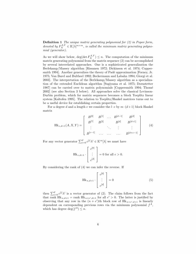
Definition 1 The unique matrix generating polynomial for (2) in Popov form,

denoted by FA,YX ∈ K [λ]m×m, is called the minimum matrix generating polyno-mial (generator).

As we will show below, deg(detFA,YX ) ≤ n. The computation of the minimummatrix generating polynomial from the matrix sequence (2) can be accomplishedby several interrelated approaches. One is a sophisticated generalization theBerlekamp/Massey algorithm [Rissanen 1972; Dickinson et al. 1974; Copper-smith 1994]. Another generalizes the theory of Pade approximation [Forney, Jr.1975; Van Barel and Bultheel 1992; Beckermann and Labahn 1994; Giorgi et al.2003]. The interpretation of the Berlekamp/Massey algorithm as a specializa-tion of the extended Euclidean algorithm [Sugiyama et al. 1975; Dornstetter1987] can be carried over to matrix polynomials [Coppersmith 1994; Thome2002] (see also Section 3 below). All approaches solve the classical Levinson-Durbin problem, which for matrix sequences becomes a block Toeplitz linearsystem [Kaltofen 1995]. The relation to Toeplitz/Hankel matrices turns out tobe a useful device for establishing certain properties.

For a degree d and a length e we consider the l ·e by m · (d+1) block Hankelmatrix

Hke,d+1(A,X, Y ) =

B[0] B[1] . . . B[d−1] B[d]

B[1] B[2] B[d] B[d+1]

.... . .

......

B[e−1] . . . . . . . . . B[d+e−1]

(4)

For any vector generator∑di=0 c

[i]λi ∈ Km[λ] we must have

Hke,d+1 ·

c[0]

...

c[d]

= 0 for all e > 0.

By considering the rank of (4) we can infer the reverse. If

Hkn,d+1 ·

c[0]

...

c[d]

= 0 (5)

then∑di=0 c

[i]λi is a vector generator of (2). The claim follows from the factthat rank Hkn,d+1 = rank Hkn+e′,d+1 for all e′ > 0. The latter is justified byobserving that any row in the (n + e′)th block row of Hkn+e′,d+1 is linearlydependent on corresponding previous rows via the minimum polynomial fA,which has degree deg(fA) ≤ n.

6

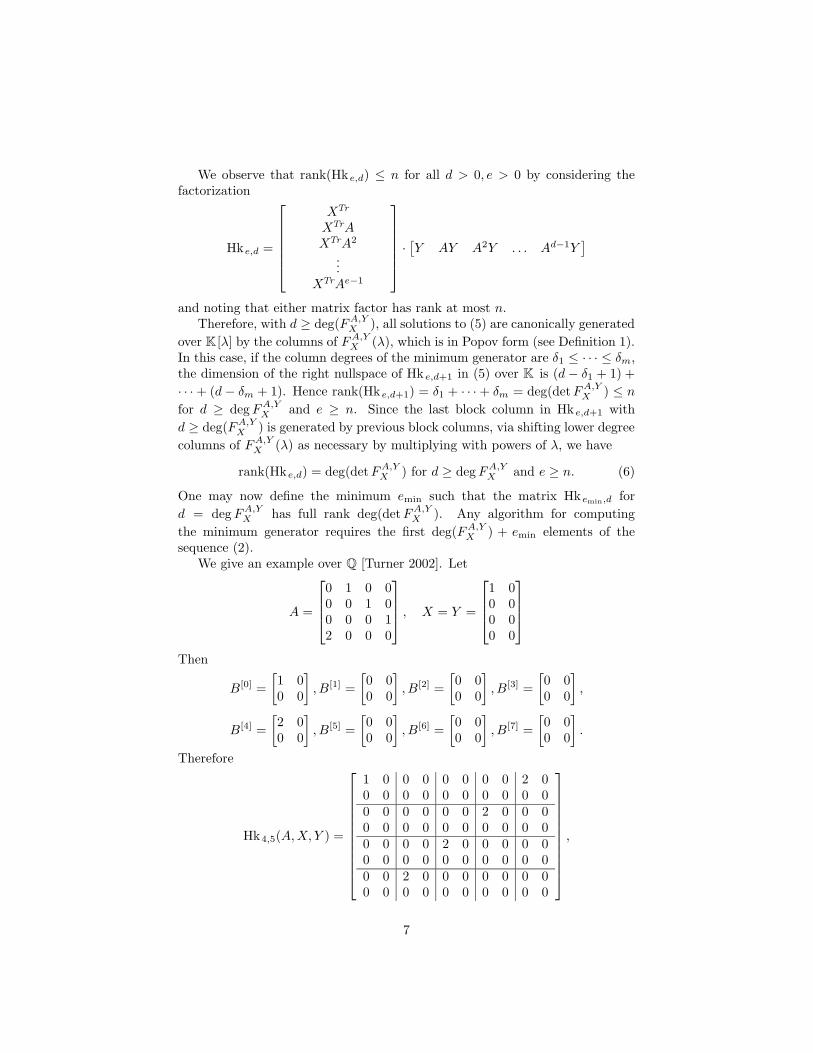
We observe that rank(Hke,d) ≤ n for all d > 0, e > 0 by considering thefactorization

Hke,d =

XTr

XTrAXTrA2

...XTrAe−1

·[Y AY A2Y . . . Ad−1Y

]

and noting that either matrix factor has rank at most n.Therefore, with d ≥ deg(FA,YX ), all solutions to (5) are canonically generated

over K [λ] by the columns of FA,YX (λ), which is in Popov form (see Definition 1).In this case, if the column degrees of the minimum generator are δ1 ≤ · · · ≤ δm,the dimension of the right nullspace of Hk e,d+1 in (5) over K is (d− δ1 + 1) +

· · ·+ (d− δm + 1). Hence rank(Hke,d+1) = δ1 + · · ·+ δm = deg(detFA,YX ) ≤ n

for d ≥ degFA,YX and e ≥ n. Since the last block column in Hk e,d+1 with

d ≥ deg(FA,YX ) is generated by previous block columns, via shifting lower degree

columns of FA,YX (λ) as necessary by multiplying with powers of λ, we have

rank(Hke,d) = deg(detFA,YX ) for d ≥ degFA,YX and e ≥ n. (6)

One may now define the minimum emin such that the matrix Hkemin,d for

d = degFA,YX has full rank deg(detFA,YX ). Any algorithm for computing

the minimum generator requires the first deg(FA,YX ) + emin elements of thesequence (2).

We give an example over Q [Turner 2002]. Let

A =

0 1 0 00 0 1 00 0 0 12 0 0 0

, X = Y =

1 00 00 00 0

Then

B[0] =

[1 00 0

], B[1] =

[0 00 0

], B[2] =

[0 00 0

], B[3] =

[0 00 0

],

B[4] =

[2 00 0

], B[5] =

[0 00 0

], B[6] =

[0 00 0

], B[7] =

[0 00 0

].

Therefore

Hk4,5(A,X, Y ) =

1 0 0 0 0 0 0 0 2 00 0 0 0 0 0 0 0 0 00 0 0 0 0 0 2 0 0 00 0 0 0 0 0 0 0 0 00 0 0 0 2 0 0 0 0 00 0 0 0 0 0 0 0 0 00 0 2 0 0 0 0 0 0 00 0 0 0 0 0 0 0 0 0

,

7

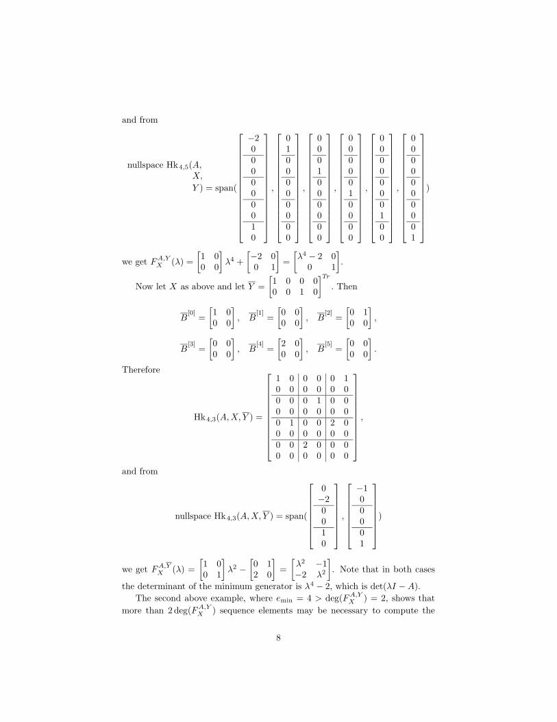
and from

nullspace Hk4,5(A,X,

Y ) = span(

−2000000010

,

0100000000

,

0001000000

,

0000010000

,

0000000100

,

0000000001

)

we get FA,YX (λ) =

[1 00 0

]λ4 +

[−2 00 1

]=

[λ4 − 2 0

0 1

].

Now let X as above and let Y =

[1 0 0 00 0 1 0

]Tr

. Then

B[0]

=

[1 00 0

], B

[1]=

[0 00 0

], B

[2]=

[0 10 0

],

B[3]

=

[0 00 0

], B

[4]=

[2 00 0

], B

[5]=

[0 00 0

].

Therefore

Hk4,3(A,X, Y ) =

1 0 0 0 0 10 0 0 0 0 00 0 0 1 0 00 0 0 0 0 00 1 0 0 2 00 0 0 0 0 00 0 2 0 0 00 0 0 0 0 0

,

and from

nullspace Hk4,3(A,X, Y ) = span(

0−20010

,

−100001

)

we get FA,YX (λ) =

[1 00 1

]λ2 −

[0 12 0

]=

[λ2 −1−2 λ2

]. Note that in both cases

the determinant of the minimum generator is λ4 − 2, which is det(λI −A).

The second above example, where emin = 4 > deg(FA,YX ) = 2, shows that

more than 2 deg(FA,YX ) sequence elements may be necessary to compute the

8

generator, in contrast to the scalar Berlekamp/Massey theory: the last block rowof Hk4,3(A,X, Y ) is required to restrict the right nullspace to the two generatingvectors.

However, for random projection block vectors X and Y both deg(FA,YX ) andemin are small. Let us define, for fixed l and m,

ν = maxd≥1,e≥1,X∈K n×l,Y ∈K n×m

{rank Hke,d(A,X, Y )}. (7)

Indeed, the probabilistic analysis [Kaltofen 1995: Section 5], [Villard 1997b:Corollary 6.4] shows the existence of matrices W ∈ Kn×l and Z ∈ Kn×m

such that the corresponding rank Hk e0,d0(A,W,Z) = ν with d0 = dν/me ande0 = dν/le. Moreover, ν is equal to the sum of the degrees of the first min{l,m}invariant factors of λI − A (see Theorem 4 below), and hence X,Y can betaken from any field extension of K . Then due to the existence of W,Z, forsymbolic entries in X,Y and therefore, by [DeMillo and Lipton 1978; Zippel1979; Schwartz 1980], for random entries, the maximal rank is preserved forblock dimensions e0, d0. Note that the degree of the minimum matrix generatingpolynomial is now deg(FA,YX ) = d0 < n/m + 1 and the number of sequenceelements required to compute the minimum generator is d0 + e0 = dν/le +dν/me < n/l + n/m + 2. If K is a small finite field, Wiedmann’s analysis hasbeen generalized in [Villard 1997b; Brent et al. 2003].

As with the unblocked Wiedemann projections, unlucky projection blockvectors X and Y may cause a drop in the determinantal degree deg(FA,YX ).They may also increase the length of the sequence required to compute thegenerator FA,YX .

2.2 Smith normal forms of matrix generating polynomials

In this section we study how the invariant structure of FA,YX partly reveals thestructure of A and λI−A. Our algorithms in Sections 4 and 5 pick random blockvectors X,Y or use special projections and compute a generator from the firstd0 + e0 elements of (2). Under the assumption that the rank of Hk e,d = ν (see

(7)) for sufficiently large d, e, we prove here that det(FA,YX ) is the product of thefirst min{l,m} invariant factors of λI − A. These are well-studied facts in thetheory of realizations of multivariable control theory, for instance see Kailath[1980]. The basis is the matrix power series

XTr(λI −A)−1Y = XTr

(∑

i≥0

Ai

λi+1

)Y =

∑

i≥0

B[i]

λi+1.

Lemma 2 One has the fraction description

XTr(λI −A)−1Y = N(λ)D(λ)−1 (8)

if and only if there exists T ∈ K [λ]m×m such that D = FA,YX T .

9

Proof. For the necessary condition, since every polynomial numerator in XTr×(λI −A)−1Y has degree strictly less than the corresponding denominator, thenevery column of N has degree strictly less than that of the corresponding columnof D. Thus it can be checked that the columns of D satisfy (3) and D must be

a multiple of FA,YX . Conversely, let D = FA,YX T in K [λ]m×m be an invertiblematrix generator for (2). Using (3) for its m columns it can be seen that wehave

XTr(λI −A)−1Y D(λ) = N(λ) ∈ K [λ]l×m

where the column degrees of N are lower than those of D. This yields the matrixfraction description (8). �

Clearly, for D = FA,YX , the minimum polynomial fA(λ) is a common de-nominator of the rational entries of the matrices on both sides of (8). If theleast common denominator of the left side matrix is actually the character-istic polynomial det(λI − A), then it follows from degree considerations that

detFA,YX = det(λI − A). Our algorithm uses the matrix preconditioners dis-cussed in Section 4 and random or ad hoc projections (Section 5) to achievethis determinantal equality. We shall make the relationship between λI−A andFA,YX more explicit in Theorem 4 whose proof will rely on the structure of thematrix denominator D in (8) and on the following.

For a square matrix M over K [λ] we consider the Smith normal form [New-man 1972], which is an equivalent diagonal matrix over K [λ] with diagonalelements s1(λ), . . ., sφ(λ), 1, . . ., 1, 0, . . . , 0, where the si’s are the nontrivial in-variant factors of M , that is, non-constant monic polynomials with the propertythat si is a (trivial or nontrivial) polynomial factor of si−1 for all 2 ≤ i ≤ φ.Because the Smith normal form of the characteristic matrix λI−A correspondsto the Frobenius canonical form of A for similarity, the largest invariant factorof λI −A, s1(λ), equals the minimum polynomial fA(λ).

Lemma 3 Let M ∈ K [λ]µ×µ be non-singular and let U ∈ K [λ]µ×µ be unimod-ular such that

MU =

[H H12

0 H22

](9)

where H is a square matrix, then the i-th invariant factor of H divides the i-thinvariant factor of M .

Proof. Identity (9) may be rewritten as

MU =

[I H12

0 H22

] [H 00 I

].

Since the invariant factors of two non-singular matrices divide the invariantfactors of their product [Newman 1972: Theorem II.14], the largest invariantfactors of diag(H, I) that are those of H, divide the corresponding invariantfactors of MU and thus M . �

We can now see how the Smith form of FA,YX is related to that of λI − A.Essentially the result may be obtained for instance following the lines of [Kailath1980: §6.4.2], we give here a statement and a proof better suited to our purposes.

10

Theorem 4 Let A ∈ Kn×n, X ∈ Kn×l, Y ∈ Kn×m and let s1, . . . , sφ denote

all invariant factors of λI − A. The i-th invariant factor of FA,YX divides si.Furthermore, there exist matrices W ∈ Kn×l and Z ∈ Kn×m such that for alli, 1 ≤ i ≤ min{l,m, φ}, the i-th invariant factor of FA,ZW is equal to si and them−min{l,m, φ} remaining ones are equal to 1. Moreover, for fixed l and m,

degλ(det(FA,ZW (λ))) = maxX,Y degλ(det(FA,YX (λ)))= deg(s1) + · · ·+ deg(smin{l,m,φ})= ν, which is defined in (7).

(10)

Proof. We prove the first statement for a particular denominator matrix D of afraction description of XTr(λI−A)−1Y . Indeed, if the i-th invariant factors of Ddivide si then, by Lemma 2 and using the product argument given in the proofof Lemma 3, the same holds by transitivity of division for FA,YX . When Y hasrank r < m, one may introduce an invertible transformation Q ∈ Km×m suchthat Y Q = [Y1 0] with Y1 ∈ Kn×r. From there, if XTr(λI −A)−1Y1 = N1D

−11

then

XTr(λI −A)−1Y =[N1(λ) 0

] [D1(λ) 0

0 I

]−1

Q−1

and the invariant factors of the denominator matrix Q diag(D1, I) are thoseof D1. We can thus without loss of generality assume that Y has full columnrank. Let us now construct a fraction description of XTr(λI − A)−1Y with Das announced. Choose Yc ∈ Kn×(n−m) such that T = [Y Yc] is invertible inKn×n and let D ∈ K [λ]m×m be defined from a unimodular triangularization ofT−1(λI −A), that is:

T−1(λI −A)U(λ) =

[D(λ) H12(λ)

0 H22(λ)

](11)

with U unimodular. If V is the matrix formed by the first m columns of U wehave the fraction descriptions (λI − A)−1Y = V D−1 and XTr(λI − A)−1Y =(XTrV

)D−1. Thus D is a denominator matrix for XTr(λI − A)−1Y . By (11)

and Lemma 3, its i-th invariant factor divide the i-th invariant factor si of λI−Aand the first assertion is proven.

To establish the rest of the theorem we work with the associated block Hankelmatrix Hke,d(A,X, Y ). By definition of the invariant factors we know that

dim span(X,ATrX, (ATr)2X, . . .) ≤ deg(s1) + · · ·+ deg(smin{l,φ})

anddim span(Y,AY,A2Y, . . .) ≤ deg(s1) + · · ·+ deg(smin{m,φ})

thus

rank Hke,d(A,X, Y ) ≤ rank (

XTr

XTrAXTrA2

...

·

[Y AY A2Y . . .

]) ≤ ν,

11

where ν = deg(s1) + · · · + deg(smin{m,l,φ}). Hence, from the specializations Wand Z of X and Y given in [Villard 1997b: Corollary 6.4], we get

rank Hke0,d0(A,W,Z) = maxX,Y,d,e

rank Hke,d+1(A,X, Y ) = ν (12)

with d0 = dν/me and e0 = dν/le and thus ν = ν. Using (6) we also have

degλ(det(FA,ZW (λ))) = maxX,Y

degλ(det(FA,YX (λ))) = ν. (13)

With (12) and (13) we have proven the two maximality assertions. In addition,

since the i-th invariant factor si of FA,ZW must divide si, the only way to get

degλ(detFA,ZW ) = ν, is to take si = si for 1 ≤ i ≤ min{m, l, φ} and si = 1 formin{m, l, φ} < i ≤ m. �

As already noticed, the existence of such W,Z establishes maximality of thematrix generator for symbolic X and Y and, by the Schwartz/Zippel lemma,

for random projection matrices. In next sections we will use detFA,ZW (λ) =det(λI − A) for computing the determinant and the characteristic polynomialof matrices A with the property φ ≤ min{l,m}. For general matrices we will

use FA,ZW to determine the first min{l,m} invariant factors of A.

3 Normal matrix polynomial remainder sequences

As done for a scalar sequence in [Sugiyama et al. 1975; Brent et al. 1980; Dorn-stetter 1987] the minimum matrix generating polynomial of a sequence canbe computed via a specialized matrix Euclidean algorithm [Coppersmith 1994;Thome 2002]. Taking advantage of fast matrix multiplication algorithms re-quires to extend these approaches. In Section 3.1 we propose a matrix Eu-clidean algorithm which combines fast matrix multiplication with the recursiveKnuth/Schonhage half-GCD algorithm [Knuth 1970; Schonhage 1971; Moenck1973; von zur Gathen and Gerhard 1999]. This is applicable to computing thematrix minimum polynomial of a sequence {XTrAY }i≥0 if the latter leads to anormal matrix polynomial remainder chain. We show in Section 3.2 that this issatisfied, with high probability, by our random integer sequences. This will besatisfied by construction by the sequence in the division-free computation. Forsimplicity we work in the square case l = m thus with a sequence {B [i]}i≥0 ofmatrices in Km×m.

3.1 Minimum polynomials and half Euclidean algorithm

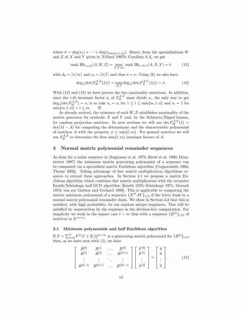
If F =∑di=0 F

[i]λi ∈ K [λ]m×m is a generating matrix polynomial for {B[i]}i≥0

then, as we have seen with (5), we have

B[0] B[1] . . . B[d]

B[1] B[2] . . . B[d+1]

......

. . ....

B[d−1] B[d+1] . . . B[2d−1]

F [0]

F [1]

...F [d]

=

00...0

. (14)

12

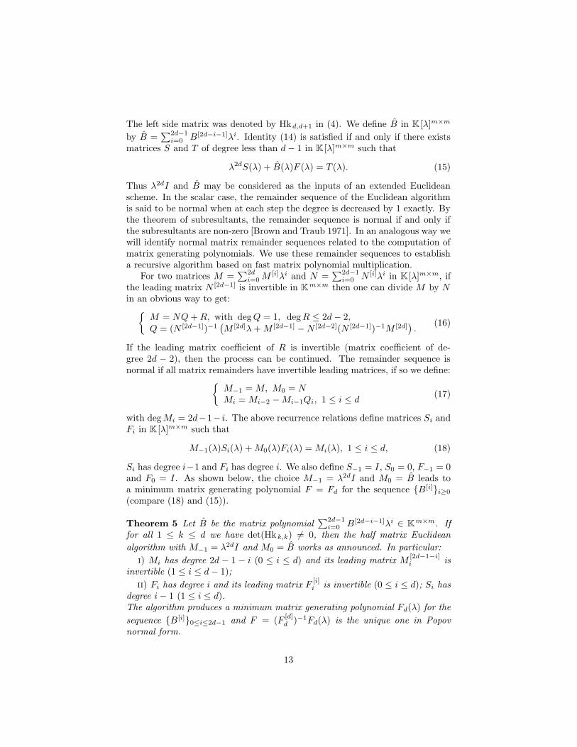
The left side matrix was denoted by Hkd,d+1 in (4). We define B in K [λ]m×m

by B =∑2d−1i=0 B[2d−i−1]λi. Identity (14) is satisfied if and only if there exists

matrices S and T of degree less than d− 1 in K [λ]m×m such that

λ2dS(λ) + B(λ)F (λ) = T (λ). (15)

Thus λ2dI and B may be considered as the inputs of an extended Euclideanscheme. In the scalar case, the remainder sequence of the Euclidean algorithmis said to be normal when at each step the degree is decreased by 1 exactly. Bythe theorem of subresultants, the remainder sequence is normal if and only ifthe subresultants are non-zero [Brown and Traub 1971]. In an analogous way wewill identify normal matrix remainder sequences related to the computation ofmatrix generating polynomials. We use these remainder sequences to establisha recursive algorithm based on fast matrix polynomial multiplication.

For two matrices M =∑2di=0M

[i]λi and N =∑2d−1i=0 N [i]λi in K [λ]m×m, if

the leading matrix N [2d−1] is invertible in Km×m then one can divide M by Nin an obvious way to get:

{M = NQ+R, with degQ = 1, degR ≤ 2d− 2,Q = (N [2d−1])−1

(M [2d]λ+M [2d−1] −N [2d−2](N [2d−1])−1M [2d]

).

(16)

If the leading matrix coefficient of R is invertible (matrix coefficient of de-gree 2d − 2), then the process can be continued. The remainder sequence isnormal if all matrix remainders have invertible leading matrices, if so we define:

{M−1 = M, M0 = NMi = Mi−2 −Mi−1Qi, 1 ≤ i ≤ d

(17)

with degMi = 2d−1− i. The above recurrence relations define matrices Si andFi in K [λ]m×m such that

M−1(λ)Si(λ) +M0(λ)Fi(λ) = Mi(λ), 1 ≤ i ≤ d, (18)

Si has degree i−1 and Fi has degree i. We also define S−1 = I, S0 = 0, F−1 = 0and F0 = I. As shown below, the choice M−1 = λ2dI and M0 = B leads toa minimum matrix generating polynomial F = Fd for the sequence {B[i]}i≥0

(compare (18) and (15)).

Theorem 5 Let B be the matrix polynomial∑2d−1i=0 B[2d−i−1]λi ∈ Km×m. If

for all 1 ≤ k ≤ d we have det(Hkk,k) 6= 0, then the half matrix Euclidean

algorithm with M−1 = λ2dI and M0 = B works as announced. In particular:

i) Mi has degree 2d − 1 − i (0 ≤ i ≤ d) and its leading matrix M[2d−1−i]i is

invertible (1 ≤ i ≤ d− 1);

ii) Fi has degree i and its leading matrix F[i]i is invertible (0 ≤ i ≤ d); Si has

degree i− 1 (1 ≤ i ≤ d).The algorithm produces a minimum matrix generating polynomial Fd(λ) for the

sequence {B[i]}0≤i≤2d−1 and F = (F[d]d )−1Fd(λ) is the unique one in Popov

normal form.

13

Furthermore, if in the half matrix Euclidean algorithm the conditions i-ii aremet for all i with 1 ≤ i ≤ d, then det(Hkk,k) 6= 0 for all 1 ≤ k ≤ d.

Proof. We prove the assertions by induction. For i = 0, since by assumptionB[0] is invertible, M0 satisfies i). By definition F0 = I and starting at i = 1,S1 = I. Now assume that the properties are true for i−1. Then, following (16),

Qi = Qiλ+ Qi =(M

[2d−i]i−1

)−1

M[2d−i+1]i−2 λ+ Qi ,

Qi is invertible by i) at previous steps and Qi is in Km×m. The leading matrixof Fi is

F[i]i = −F

[i−1]i−1 Qi

thus Fi satisfies ii). The same argument holds for Si (i−1 ≥ 1). By constructionMi has a degree lower than 2d− 1− i hence, looking at the right side coefficientmatrices of (18), we know that

B[0] B[1] . . . B[i]

B[1] B[2] . . . B[i+1]

......

. . ....

B[i] B[i+1] . . . B[2i]

︸ ︷︷ ︸Hk i+1,i+1

F[0]i

F[1]i...

F[i]i

=

00...

M[2d−1−i]i

. (19)

By assumption of non-singularity of Hk i+1,i+1 and since we have proved that

F[i]i is invertible, the columns in the right side matrix of (19) are linearly inde-

pendent, thus M[2d−1−i]i is invertible. This proves i). Identity (18) for i = d

also establishes (14) which means that Fd is a matrix generating polynomial

for {B[i]}0≤i≤2d−1 whose leading matrix F[d]d its invertible. It follows that

F = (F[d]d )−1Fd(λ) is in Popov normal form. The minimality comes from the

fact that Hkd,d is invertible and hence no vector generator (column of a matrixgenerator) can be of degree less than d.

We finally prove that invertible leading coefficient matrices in the Euclideanalgorithm guarantee non-singularity for all Hkk,k. To that end, we consider therange of Hk i+1,i+1 in (19). Clearly, the block vector [ 0 Im]Tr is in the range,

since M[2d−1−i]i is invertible. By induction hypothesis for Hk i,i, we see that the

first i block columns of Hk i+1,i+1 can generate [ Imi 0 ]Tr, where the block zerorow at the bottom is achieved by subtraction of appropriate linear combinationsof the previous block vector [ 0 Im]Tr. Hence the range of Hk i+1,i+1 has fulldimension. �

For B[i] = XTrAY , i ≥ 0, the next corollary shows that F is as expected.

Corollary 6 Let A be in Kn×n, let B[i] = XTrAiY ∈ Km×m, i ≥ 0, and letν = md be the determinantal degree degλ(detFA,YX ). If the block Hankel matrix

Hkd,d(A,X, Y ) satisfies the assumption of Theorem 5 then F = FA,YX .

14

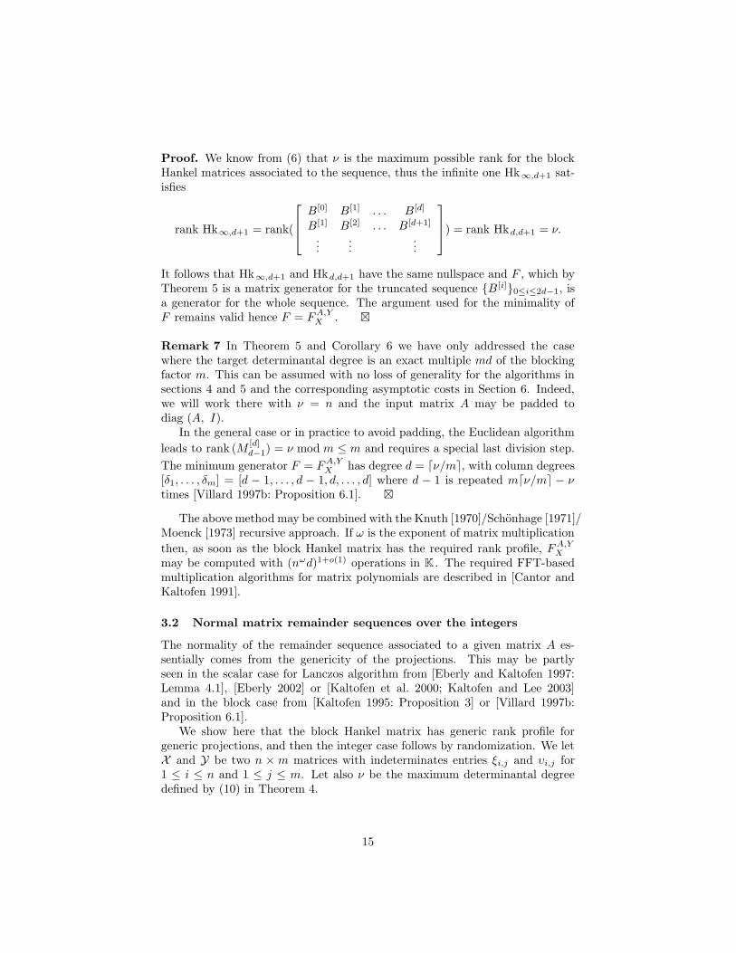
Proof. We know from (6) that ν is the maximum possible rank for the blockHankel matrices associated to the sequence, thus the infinite one Hk∞,d+1 sat-isfies

rank Hk∞,d+1 = rank(

B[0] B[1] . . . B[d]

B[1] B[2] . . . B[d+1]

......

...

) = rank Hkd,d+1 = ν.

It follows that Hk∞,d+1 and Hkd,d+1 have the same nullspace and F , which byTheorem 5 is a matrix generator for the truncated sequence {B [i]}0≤i≤2d−1, isa generator for the whole sequence. The argument used for the minimality ofF remains valid hence F = FA,YX . �

Remark 7 In Theorem 5 and Corollary 6 we have only addressed the casewhere the target determinantal degree is an exact multiple md of the blockingfactor m. This can be assumed with no loss of generality for the algorithms insections 4 and 5 and the corresponding asymptotic costs in Section 6. Indeed,we will work there with ν = n and the input matrix A may be padded todiag (A, I).

In the general case or in practice to avoid padding, the Euclidean algorithm

leads to rank (M[d]d−1) = ν mod m ≤ m and requires a special last division step.

The minimum generator F = FA,YX has degree d = dν/me, with column degrees[δ1, . . . , δm] = [d − 1, . . . , d − 1, d, . . . , d] where d − 1 is repeated mdν/me − νtimes [Villard 1997b: Proposition 6.1]. �

The above method may be combined with the Knuth [1970]/Schonhage [1971]/Moenck [1973] recursive approach. If ω is the exponent of matrix multiplication

then, as soon as the block Hankel matrix has the required rank profile, FA,YX

may be computed with (nωd)1+o(1) operations in K . The required FFT-basedmultiplication algorithms for matrix polynomials are described in [Cantor andKaltofen 1991].

3.2 Normal matrix remainder sequences over the integers

The normality of the remainder sequence associated to a given matrix A es-sentially comes from the genericity of the projections. This may be partlyseen in the scalar case for Lanczos algorithm from [Eberly and Kaltofen 1997:Lemma 4.1], [Eberly 2002] or [Kaltofen et al. 2000; Kaltofen and Lee 2003]and in the block case from [Kaltofen 1995: Proposition 3] or [Villard 1997b:Proposition 6.1].

We show here that the block Hankel matrix has generic rank profile forgeneric projections, and then the integer case follows by randomization. We letX and Y be two n × m matrices with indeterminates entries ξi,j and υi,j for1 ≤ i ≤ n and 1 ≤ j ≤ m. Let also ν be the maximum determinantal degreedefined by (10) in Theorem 4.

15

Lemma 8 With d = dν/me, the block Hankel matrix Hkd,d(A,X ,Y) has rankν and its principal minors of order i are non-zero for 1 ≤ i ≤ ν.

Proof. For simplifying the presentation we only detail the case where ν is amultiple of m (see Remark 7). Let Kr i(A,Z) ∈ Kn×i be the block Krylovmatrix formed by the i first columns of [Z AZ . . . Ad−1Z] for 1 ≤ i ≤ ν. Thespecialization Z ∈ Kn×m of Y given in [Villard 1997b: Proposition 6.1] satisfies

rank Kr i(A,Z) = i, 1 ≤ i ≤ ν. (20)

We now argue, by specializing X and Y, that the target principal minors arenon-zero. If i ≤ m, using (20) one can find X ∈ Kn×i such that the rankof XTrKr i(A,Z) equals i. If m < i ≤ ν then one can find X ∈ Kn×m suchthat XTrKr i(A,Z) = [0 Jm] where Jm is the m ×m reversion matrix. HenceHkd,d(A,X,Z) has ones on its ith anti-diagonal and zeros above, the corre-sponding principal minor of order i is (−1)i. �

The polynomial∏dk=1 det(Hkk,k(A,X ,Y)) is non-zero of degree no more

md(d+ 1) in K [. . . , ξi,j , . . . , υi,j , . . .]. If the entries of X and Y are chosen uni-formly and independently from a finite set S ⊂ Z then, by the Schwartz/Zippellemma and Theorem 5, the associated matrix remainder sequence is normalwith probability at least 1−md(d+ 1)/|S|.

4 The block baby steps/giant steps determinant algorithm

We shall present our algorithm for integer matrices. Generalizations to otherdomains, such as polynomial rings, are certainly possible. The algorithm fol-lows the Wiedemann paradigm [Wiedemann 1986: Chapter V] and uses a babysteps/giant steps approach for computing the sequence elements [Kaltofen 1992].In addition, the algorithm blocks the projections [Coppersmith 1994]. A key in-gredient is that from the theory of realizations described in Section 2, it ispossible to recover the characteristic polynomial of a preconditioning of theinput matrix.

Algorithm Block Baby Steps/Giant Steps Determinant

Input: a matrix A ∈ Zn×n.Output: an integer that is the determinant of A, or “failure;” the algorithm failswith probability no more than 1/2.

Step 0. Let h = log2 Hd(A), where Hd(A) is a bound on the magnitude of thedeterminant of A, for instance, Hadamard’s bound (see, for example, [vonzur Gathen and Gerhard 1999]). For purpose of guaranteeing the prob-ability of a successful completion, the algorithm uses positive constantsγ1, γ

′1 ≥ 1.

Choose a random prime integer p0 ≤ γ′1hγ1 and compute det(A) mod p0

by LU-decomposition over Zp0 .If the result is zero, A is most likely singular, and the algorithm calls an

16

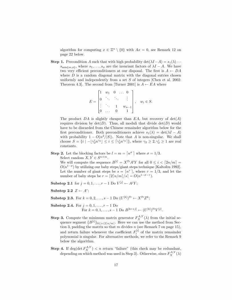
algorithm for computing x ∈ Zn \ {0} with Ax = 0, see Remark 12 onpage 22 below.

Step 1. Precondition A such that with high probability det(λI−A) = s1(λ) · · ·smin{m,φ}, where s1, . . . , sφ are the invariant factors of λI − A. We havetwo very efficient preconditioners at our disposal. The first is A ← DAwhere D is a random diagonal matrix with the diagonal entries chosenuniformly and independently from a set S of integers [Chen et al. 2002:Theorem 4.3]. The second from [Turner 2001] is A← EA where

E =

1 w1 0 . . . 0

0. . .

. . ....

.... . . 1 wn−1

0 . . . 0 1

, wi ∈ S.

The product DA is slightly cheaper than EA, but recovery of det(A)requires division by det(D). Thus, all moduli that divide det(D) wouldhave to be discarded from the Chinese remainder algorithm below for thefirst preconditioner. Both preconditioners achieve s1(λ) = det(λI − A)with probability 1 − O(n2/|S|). Note that A is non-singular. We shallchoose S = {i | −bγ′2n

γ2c ≤ i ≤ dγ′2nγ2e}, where γ2 ≥ 2, γ′2 ≥ 1 are real

constants.

Step 2. Let the blocking factors be l = m = dnσ e where σ = 1/3.Select random X,Y ∈ Sn×m.We will compute the sequence B[i] = XTrAiY for all 0 ≤ i < d2n/me =O(n1−σ) by utilizing our baby steps/giant steps technique [Kaltofen 1992].Let the number of giant steps be s = dnτ e, where τ = 1/3, and let thenumber of baby steps be r = d2dn/me/se = O(n1−σ−τ ).

Substep 2.1 for j = 0, 1, . . . , r − 1 Do V [j] ← AjY ;

Substep 2.2 Z ← Ar;

Substep 2.3. For k = 0, 2, . . . , s− 1 Do (U [k])Tr ← XTrZk;

Substep 2.4. For j = 0, 1, . . . , r − 1 DoFor k = 0, 1, . . . , s− 1 Do B[kr+j] ← (U [k])TrV [j].

Step 3. Compute the minimum matrix generator FA,YX (λ) from the initial se-quence segment {B[i]}0≤i<2dn/me. Here we can use the method from Sec-tion 3, padding the matrix so that m divides n (see Remark 7 on page 15),

and return failure whenever the coefficient F[i]i of the matrix remainder

polynomial is singular. For alternative methods, we refer to the Remark 9below the algorithm.

Step 4. If deg(detFA,YX ) < n return “failure” (this check may be redundant,

depending on which method was used in Step 3). Otherwise, since FA,YX (λ)

17

is in Popov form we know that its determinant is monic and by Theorem 4we have detFA,YX (λ) = det(λI −A). Return det(A) = ∆(0). �

Remark 9 As we have seen in Section 2.1 there are several alternatives forcarrying out Step 3 [Rissanen 1972; Dickinson et al. 1974; Forney, Jr. 1975;Van Barel and Bultheel 1992; Beckermann and Labahn 1994; Kaltofen 1995;Coppersmith 1994; Thome 2002; Giorgi et al. 2003]. In Step 4 we require that

detFA,YX (λ) = det(λI − A). In order to achieve the wanted bit complexity, wemust stop any of the algorithms after having processed the first 2dn/me elements

of (2). The used algorithm then must return a candidate matrix polynomial F .

Clearly, if Step 4 exposes deg(det F ) < n one knows that the randomizations

were unlucky. However, if deg(det F ) = n there still may be the possibility that

F 6= FA,YX due to a situation where the first 2dn/me elements do not determinethe generator, as would be the case in the two examples given in Section 2. Inorder to achieve the Las Vegas model of randomized algorithmic complexity,verification of the computed generator is thus necessary here. For example, theused algorithm could do so by establishing that rankHk dn/me,dn/me(A,X, Y ) =n. Our algorithm from Section 3 implicitly does so via Theorem 5 on page 13.One could do so explicitly be computing the rank of Hk dn/me,dn/me modulo arandom prime number.

We remark that the arithmetic cost of verifying that the candidate for FA,YX

is a generator for the block Krylov sequence {AiY }i≥0 is the same as step 2.The reduction is seen by applying the transposition principle [Kaltofen 2000:Section 6]: note that computing all B[i] is the block diagonal left product

[(XTr)1,∗ | (X

Tr)2,∗ | . . .]·

. . . AiY . . . 0 0 · · · 00 . . . AiY . . . 0 · · · 0...

. . ....

0 0 · · · . . . AiY . . .

,

where (XTr)i,∗ denotes the i-th row of XTr. Computing∑iA

iY c[i], where

c[i] ∈ Km×m are the coefficients of FA,YX , is the block diagonal right product

. . . AiY . . . 0 0 · · · 00 . . . AiY . . . 0 · · · 0...

. . ....

0 0 · · · . . . AiY . . .

·

(c[0])∗,1(c[1])∗,1

...(c[0])∗,2(c[1])∗,2

...

,

where (c[i])∗,j denotes the j-th column of the matrix c[i]. One may also developan explicit baby steps/giant steps algorithm for computing

∑iA

iY c[i]. How-ever, because the integer lengths of the entries in c[i] are much larger than thoseof X and Y , we do not know how to keep the bit complexity low enough to

18

allow verification of the candidate generator via verification as a block Krylovspace generator. �

We shall first give the bit complexity analysis for our block algorithm underthe assumption that no subcubic matrix multiplication a la Strassen or sub-quadratic block Toeplitz solver/greatest common divisor algorithm a la Knuth/Schonhage is employed. We will investigate those best theoretically possiblerunning times in Section 6.

Theorem 10 Our algorithm computes the determinant of any non-singularmatrix A ∈ Zn×n with (n3+1/3 log ‖A‖)1+o(1) bit operations. Our algorithmutilizes (n1+1/3 + n log ‖A‖)1+o(1) random bits and either returns the correctdeterminant or it returns “failure,” the latter with probability of no more than1/2.

In our analysis, we will use modular arithmetic. The following lemma will beused to establish the probability of getting a good reduction with prime moduli.

Lemma 11 Let γ ≥ 1, γ′ ≥ 1 be positive real constants. Then for all integersH ∈ Z≥2 that with h = loge(H)/0.84 ≤ 1.72 log2(H) satisfy h ≥ 114 andγ′ ≤ hγ the probability

Prob(p divides H | p a prime integer, 2 ≤ p ≤ γ ′hγ) ≤5

2

γ

γ′hγ−1. (21)

Proof. We have the following estimates for the distribution of prime numbers:

∏

p primep≤x

p > eC1x, π(x) =∑

p primep≤x

1 >C2x

loge x, π(x) <

C3x

loge x

where C1, C2 and C3 are positive constants. Explicit values for C1, C2 and C3

have been derived. It is shown in [Rosser and Schoenfeld 1962] that we maychoose C1 = 0.84 for x ≥ 101, C2 = 1 for x ≥ 17, and C3 = 1.25 for x ≥ 114.

Since we have∏p≤h p > eC1h = H, there are at most π(h) < C3h/(loge h)

distinct prime factors in H. The number of primes ≤ γ ′hγ is more thanC2γ

′hγ/(γ loge h+ loge γ′), because from our assumptions we have that γ ′hγ ≥

114 > 17. Therefore the probability for a random p to divide H is no morethan, using loge γ

′ ≤ γ loge h,

C3h/(loge h)

C2γ′hγ/(γ loge h+ loge γ′)≤

C3h/(loge h)

C2γ′hγ/(2γ loge h)≤

5

2

γ

γ′hγ−1. �

In the above Lemma 11 we have introduced the constant γ ′ so that it ispossible to choose γ = 1 and have a positive probability of avoiding a primedivisor of H.

Proof of Theorem 10. The unblocked version of the algorithm is fully ana-lyzed in [Kaltofen 2002] with the additional modification of early termination

19

when the determinant is small. That analysis uses a residue number system(Chinese remaindering) for representing long integers, which we adopt for theblocked algorithm. This adds the bit cost of generating a stream of sufficientlylarge random primes (including p0 in Step 0).

Step 0 has by h = O(n log(n‖A‖)), which follows from Hadamard’s bound,the bit complexity (n3 + n2 log ‖A‖)1+o(1), the latter term constituting takingevery entry of A modulo p0. The failure probabily of Step 0, that is whendet(A) ≡ 0 (mod p0) for non-singular A, is bounded by Lemma 11. Thus, forH = det(A) and appropriate choice of γ1 and γ′1 in Step 0 all non-singularmatrices will pass with probability no less than 9/10.

Step 1 increases log ‖DA‖ or log ‖EA‖ to no more than O((log n)2 log ‖A‖)and has bit cost (n3 log ‖A‖)1+o(1).

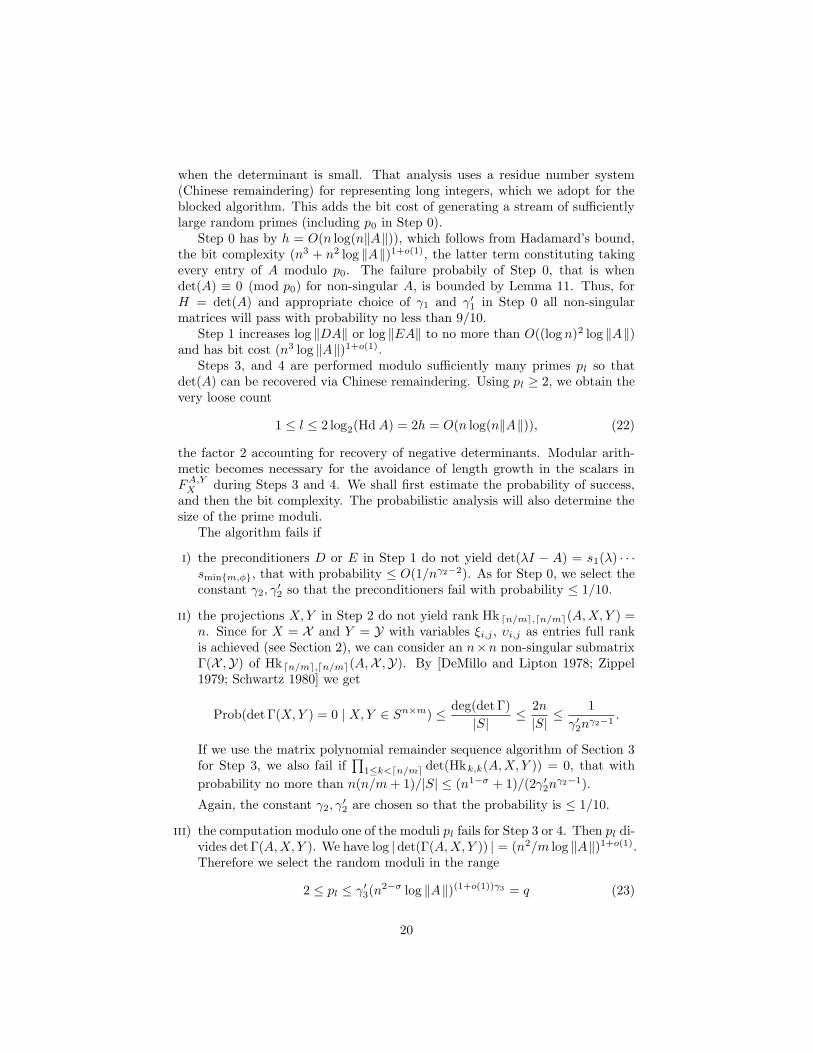
Steps 3, and 4 are performed modulo sufficiently many primes pl so thatdet(A) can be recovered via Chinese remaindering. Using pl ≥ 2, we obtain thevery loose count

1 ≤ l ≤ 2 log2(HdA) = 2h = O(n log(n‖A‖)), (22)

the factor 2 accounting for recovery of negative determinants. Modular arith-metic becomes necessary for the avoidance of length growth in the scalars inFA,YX during Steps 3 and 4. We shall first estimate the probability of success,and then the bit complexity. The probabilistic analysis will also determine thesize of the prime moduli.

The algorithm fails if

i) the preconditioners D or E in Step 1 do not yield det(λI − A) = s1(λ) · · ·smin{m,φ}, that with probability ≤ O(1/nγ2−2). As for Step 0, we select theconstant γ2, γ

′2 so that the preconditioners fail with probability ≤ 1/10.

ii) the projections X,Y in Step 2 do not yield rank Hk dn/me,dn/me(A,X, Y ) =n. Since for X = X and Y = Y with variables ξi,j , υi,j as entries full rankis achieved (see Section 2), we can consider an n×n non-singular submatrixΓ(X ,Y) of Hkdn/me,dn/me(A,X ,Y). By [DeMillo and Lipton 1978; Zippel1979; Schwartz 1980] we get

Prob(det Γ(X,Y ) = 0 | X,Y ∈ Sn×m) ≤deg(det Γ)

|S|≤

2n

|S|≤

1

γ′2nγ2−1

.

If we use the matrix polynomial remainder sequence algorithm of Section 3for Step 3, we also fail if

∏1≤k<dn/me det(Hkk,k(A,X, Y )) = 0, that with

probability no more than n(n/m+ 1)/|S| ≤ (n1−σ + 1)/(2γ′2nγ2−1).

Again, the constant γ2, γ′2 are chosen so that the probability is ≤ 1/10.

iii) the computation modulo one of the moduli pl fails for Step 3 or 4. Then pl di-vides det Γ(A,X, Y ). We have log |det(Γ(A,X, Y )) | = (n2/m log ‖A‖)1+o(1).Therefore we select the random moduli in the range

2 ≤ pl ≤ γ′3(n

2−σ log ‖A‖)(1+o(1))γ3 = q (23)

20

where σ = 1/3 and γ3 ≥ 2, γ′3 ≥ 1 are constants. Note that in (23) theexponent (1+o(1)) captures derivable polylogarithmic factors C1(log n)C2 ×(log ‖A‖)C3 , where C1, C2, C3 are explicit constants. By Lemma 11 theprobability that any one of the≤ 2hmoduli fails, i.e. divides det(Γ(A,X, Y )),is no more than 2h/(n2−σ log ‖A‖)(1+o(1))(γ3−1). By the Hadamard estimate(22) we can make this probability no larger than 1/10 via selecting theconstants γ3, γ

′3 sufficiently large.

If we also must avoid divisors of∏

1≤k<dn/me det(Hkk,k(A,X, Y )) for the

matrix polynomial remainder sequence algorithm, the range (23) increasesto pl ≤ γ

′3(n

3−2σ log ‖A‖)(1+o(1))γ3 .

iv) the algorithms fails to compute sufficiently many random prime modulipl ≤ q (see (23)). There is now a deterministic algorithm of bit complexity(log pl)

12+o(1) for primality testing [Agrawal et al. 2002], which is not re-quired but simplifies the theoretical analysis here. We pick k = 4h log q pos-itive integers≤ q. The probability for each to be prime is≥ 1/ log q = ψ (pro-vided q ≥ 17 [Rosser and Schoenfeld 1962]). By Chernoff bounds for the tailof the binomial distribution, the probability that fewer than 2h = (1−1/2)ψk

are prime is ≤ e−(1/2)2ψk/2 = 1/eh/2. Thus for h ≥ 5 the probability of fail-ing to find 2h primes is ≤ 1/10.

The cases i-iv together with Step 0 add up to a failure probability of ≤ 1/2.We conclude by estimating the number of bit operations for Steps 2-4.

Step 2 computes B[i] mod pl for 0 ≤ i < 2dn/me and 1 ≤ l ≤ 2h as follows.First, all B[i] are computed as exact integers. For substeps 2.1 and 2.2 that re-quires O(n3 log r) arithmetic operations on integers of length (r log ‖A‖)1+o(1),in total (n4−σ−τ log ‖A‖)1+o(1) bit operations (recall that σ = τ = 1/3). Sub-steps 2.3 and 2.4 require O(smn2) arithmetic operations on integers of length(r s log ‖A‖)1+o(1), again (n3+τ log ‖A‖)1+o(1) bit operations. Then allO(n/m×m2) entries of all B[i] are taken modulo pl with l in the range (22) and pl in (23).Straight-forward remaindering would yield a total of (nmh rs log ‖A‖)1+o(1)

bit operations, which is (n3(log ‖A‖)2)1+o(1). The complexity can be reducedto (n3 log ‖A‖)1+o(1) via a tree evaluation scheme [Heindel and Horowitz 1971;Aho et al. 1974: Algorithm 8.4].†

Steps 3 and 4 are performed modulo allO(h) prime moduli pl. For each primethe cost of extended Euclidean algorithm on matrix polynomials isO(m3(n/m)2)residue operations. Overall, the bit complexity of Steps 3 and 4 is again(n3+σ log ‖A‖)1+o(1). The number of required random bits in D or E, X and Y ,and case iv above is immediate. �

It is possible to derive explicit values for the constants γ1, γ′1, γ2, γ

′2, γ3, and

γ′3 so that Theorem 10 holds. However, any implementation of the algorithmwould select reasonably small values. For example, all prime moduli would bechosen 32 or 64 bit in length. Since the method is Las Vegas, such choice onlyeffects the probability of not obtaining a result.

†Note that this speedup comes at a cost of an extra log-factor.

21

If Step 3 uses a Knuth/Schonhage half-GCD approach with FFT-based poly-nomial arithmetic for the Euclidean algorithm on matrix polynomials of Sec-tion 3, the complexity for each modulus reduces to (m2n)1+o(1) residue op-erations. Thus, the overall complexity of Steps 3 and 4 reduces to (n2+2σ ×log ‖A‖)1+o(1) bit operations. For σ = 3/5 and τ = 1/5 the bit complexity ofthe algorithm then is (n3+1/5 log ‖A‖)1+o(1) (cf. [Kaltofen and Villard 2004] and[Pan 2002]).

Remark 12 In order to state a Las Vegas bit complexity for the determinantof a general square matrix, we need to consider the cost of certifying singularityin Step 0 on page 16 above. In order to meet the complexity of Theorem 10 onpage 19 above we can use the algorithm in [Dixon 1982]. Reduction to a non-singular subproblem can be accomplished by methods in [Kaltofen and Saunders1991], and the rank is determined in a Monte Carlo manner via a random primemodulus; see also [Villard 1988: page 102].

5 Improved division-free complexity

Our baby steps/giant steps algorithm with blocking of Section 4 can be em-ployed to improve the division-free complexity of the determinant of [Kaltofen1992]. Here we consider a matrix A ∈ Rn×n, where R is a commutative ringwith a unit element. At task is to compute the determinant of A by ring ad-ditions, subtractions and multiplications. Blocking can improve the numberof ring operations from n3.5+o(1) [Kaltofen 1992] to n3+1/3+o(1), that withoutsubcubic matrix multiplication or subquadratic Toeplitz/GCD algorithms, andbest possible from O(n3.0281) [Kaltofen 1992]‡ to O(n2.6973). Our algorithmcombines the blocked determinant algorithm with the elimination of divisionstechnique of [Kaltofen 1992]. Our computational model is either a straight-lineprogram/arithmetic circuit or an algebraic random access machine [Kaltofen1988]. Further problems are to compute the characteristic polynomial and theadjoint matrix of A.

The main idea of [Kaltofen 1992] follows [Strassen 1973] and for the inputmatrix A computes the determinant of the polynomial matrix L(z) = M+z(A−M), where M ∈ Zn×n is an integral matrix whose entries are independent of theentries in A. For ∆(z) = det(L(z)) we have det(A) = ∆(1). All intermediateelements are represented as polynomials in R[z] or as truncated power seriesin R[[z]] and the “shift” matrix M determines them in such a manner thatwhenever a division by a polynomial or truncated power series is performed theconstant coefficients are ±1. For the algorithm in Section 4 we not only pickM but also concrete projection block vectors X ∈ Zn×m and Y ∈ Zn×m. Norandomization is necessary, as M is a “good” input matrix (φ = m) and X and

Y are “good” projections, we have detFL(z),YX (λ) = det(λI − L(z)).

‡The proceedings paper gives an exponent 3.188; the smaller exponent is in a postnoteadded to the version posted on www.kaltofen.us/bibliography.

22

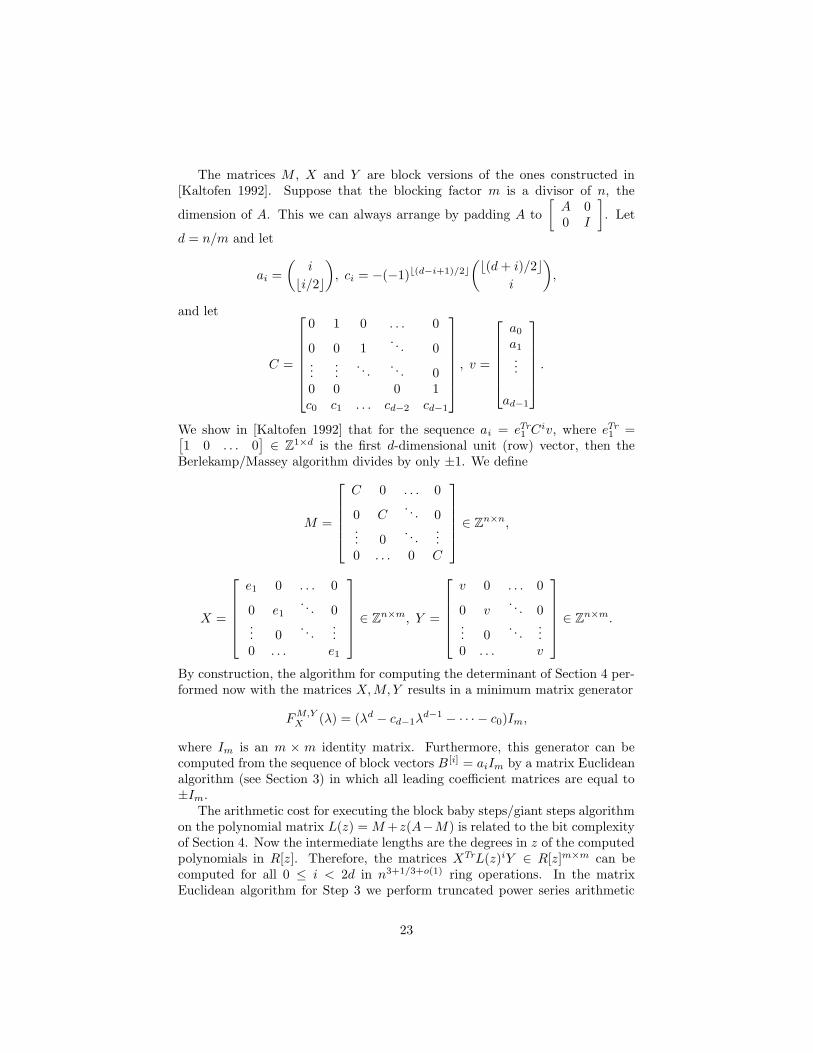
The matrices M , X and Y are block versions of the ones constructed in[Kaltofen 1992]. Suppose that the blocking factor m is a divisor of n, the

dimension of A. This we can always arrange by padding A to

[A 00 I

]. Let

d = n/m and let

ai =

(i

bi/2c

), ci = −(−1)b(d−i+1)/2c

(b(d+ i)/2c

i

),

and let

C =

0 1 0 . . . 0

0 0 1. . . 0

......

. . .. . . 0

0 0 0 1c0 c1 . . . cd−2 cd−1

, v =

a0

a1

...

ad−1

.

We show in [Kaltofen 1992] that for the sequence ai = eTr

1 Civ, where eTr

1 =[1 0 . . . 0

]∈ Z1×d is the first d-dimensional unit (row) vector, then the

Berlekamp/Massey algorithm divides by only ±1. We define

M =

C 0 . . . 0

0 C. . . 0

... 0. . .

...0 . . . 0 C

∈ Zn×n,

X =

e1 0 . . . 0

0 e1. . . 0

... 0. . .

...0 . . . e1

∈ Zn×m, Y =

v 0 . . . 0

0 v. . . 0

... 0. . .

...0 . . . v

∈ Zn×m.

By construction, the algorithm for computing the determinant of Section 4 per-formed now with the matrices X,M, Y results in a minimum matrix generator

FM,YX (λ) = (λd − cd−1λ

d−1 − · · · − c0)Im,

where Im is an m × m identity matrix. Furthermore, this generator can becomputed from the sequence of block vectors B [i] = aiIm by a matrix Euclideanalgorithm (see Section 3) in which all leading coefficient matrices are equal to±Im.

The arithmetic cost for executing the block baby steps/giant steps algorithmon the polynomial matrix L(z) = M+z(A−M) is related to the bit complexityof Section 4. Now the intermediate lengths are the degrees in z of the computedpolynomials in R[z]. Therefore, the matrices XTrL(z)iY ∈ R[z]m×m can becomputed for all 0 ≤ i < 2d in n3+1/3+o(1) ring operations. In the matrixEuclidean algorithm for Step 3 we perform truncated power series arithmetic

23

modulo zn+1. The arithmetic cost is (d2m3n)1+o(1) ring operations for theclassical Euclidean algorithm with FFT-based power series arithmetic. For thelatter, we employ a division-free FFT-based polynomial multiplication algorithm[Cantor and Kaltofen 1991]. Finally, for obtaining the characteristic polynomial,we may slightly extend Step 4 on page 17 and compute the entire determinant

of FL(z),YX (λ) division-free in truncated power series arithmetic over R[z, λ] mod

(zn+1, λn+1). For this last step we can use our original division-free algorithm[Kaltofen 1992] and achieve arithmetic complexity (m3.5n2)1+o(1). We haveproven the following theorem.

Theorem 13 Our algorithm computes the characteristic polynomial of any ma-trix A ∈ Rn×n with (n3+1/3)1+o(1) ring operations in R. By the results in [Baurand Strassen 1983] the same complexity is obtained for the adjoint matrix, whichcan be symbolically defined as det(A)A−1.

6 Using fast matrix multiplication

As stated in the Introduction, by use of sub-cubic matrix multiplication algo-rithms the worst case bit complexity of the block algorithms in Section 4 and 5can be brought below cubic complexity in n. We note that taking the n2 entriesof the input matrix modulo n prime residues is already a cubic process in n; ouralgorithms therefore proceed differently.

Now let ω by the exponent for fast matrix multiplication. By [Coppersmithand Winograd 1990] we may set ω = 2.375477. The considerations in thissection are of a purely theoretical nature.

Substep 2.1 in Section 4 is done by repeated doubling as in[A2µ

Y A2µ+1Y . . . A2µ+1−1Y]

= A2µ[Y AY . . . A2µ−1

Y]

for µ = 0, 1, . . .

Therefore the bit complexity for Substeps 2.1 and 2.2 is (nωr log ‖A‖)1+o(1) withan exponent ω + 1 − σ − τ for n. Note that σ and τ determine the blockingfactor and number of giant steps, and will be chosen later so as to minimize thecomplexity.

Substep 2.3 both splits the integer entries in U [k] into chunks of length(r log ‖A‖)1+o(1), which is the bit length of the entries in Z. There are at mosts1+o(1) such chunks. Thus each block vector times matrix product (U [k])TrZ isa rectangular matrix product of dimensions (ms)1+o(1) × n by n × n. We nowappeal to fast methods for rectangular matrices [Coppersmith 1997] (we seemnot to need the results in [Huang and Pan 1998]), which show how to multiplyan n× n matrix by an n × ν matrix in nω−θ+o(1)νθ+o(1) arithmetic operations(by blocking the n×n matrix into (t× t)-sized blocks and the n× ν matrix into(t×tζ)-sized blocks such that n/t = ν/tζ and that the individual block productsonly take t2+o(1) arithmetic steps each), where θ = (ω − 2)/(1− ζ) with ζ =0.2946289. There are s such products on integers of length (r log ‖A‖)1+o(1),so the bit complexity for Substep 2.3 is (snω−θ(ms)θr log ‖A‖)1+o(1) with anexponent ω + 1− σ + (σ + τ − 1)θ for n.

24

ω ζ η σ τ

1 ω ζ ω + 1−ζω2−(2+ζ)ω+2 1− ω−(1+ζ)

ω2−(2+ζ)ω+2ω−2

ω2−(2+ζ)ω+2

2 2.375477 0.2946289 2.697263 0.506924 0.171290

3 ω 0 ω + 1(ω−1)2+1 1− ω−1

(ω−1)2+1ω−2

(ω−1)2+1

4 3 0 3 + 15

35

15

5 log2(7) 0 3.041738 0.576388 0.189230

6 2.375477 0 2.721267 0.524375 0.129836

7 2 0 2 + 12

12 0

Table 1: Determinantal bit/division-free complexity exponent η.

Step 3 for each individual modulus can be performed by the method pre-sented in Section 3 in (mωn/m)1+o(1) residue operations. For all ≤ 2h moduliwe get a total bit complexity for Step 3 of (mω−1n2 log ‖A‖)1+o(1) with anexponent 2 + σ(ω − 1) for n.

The bit complexities of Substep 2.4 and Step 4 are dominated by the com-plexities of other steps.

All of the above bit costs lead to total bit complexity of (nη log ‖A‖)1+o(1)

where the exponent η depends on the use matrix multiplication exponents ωand ζ. Table 1 displays the optimal values of η for selected exponents togetherwith the exponents for the blocking factor and giant stepping that achieve theoptimum. Line 1 is the symbolic solution, Line 2 gives the best exponent thatwe have achieved. Line 3 is the solution without appealing to faster rectangu-lar matrix multiplication schemes. Line 4 corresponds to the comments beforeRemark 12 on page 22, and Line 5 uses Strassen’s original subquadratic matrixmultiplication algorithm. Line 6 exhibits the slowdown without faster rectangu-lar matrix multiplication algorithms. Line 7 is our complexity for a hypotheticalquadratic matrix multiplication algorithm.

An issue arises whether the singularity certification in Step 0 of our algorithmcan be accomplished at a matching or lower bit complexity than the ones givenabove for the determinant. We refer to possible approaches in [Mulders andStorjohann 2000; Storjohann 2003].

The above analysis applies to our algorithm in Section 5 and yields for thedeterminant and adjoint matrix a division-free complexity of O(n2.697263) ringoperations. To our knowledge, this is the best-known to-date. A complicationarises in Step 4 when the entire characteristic polynomial is to be computed

without divisions. The computation of detFL(z),YX (λ) mod (zn+1, λn+1) seems

to require O(mω) operations modulo (zn+1, λn+1).§ We note that for λ = z = 0the generator matrix polynomial evaluates to Im, so asymptotically fast LU-decomposition algorithms are applicable [Aho et al. 1974]. Step 4 now needs

§It may be possible to take advantage of degλ FL(z),YX

(λ) = n/m, but currently we do notknow how.

25

(nσω+2)1+o(1) ring operations, reducing the division-free complexity for the char-

acteristic polynomial to nχ+o(1), χ = ω + 2(1−ζ)ω2−(1+ζ)ω+1−ζ ring operations. We

obtain with ω = 2.375477 and ζ = 0.2946289 at σ ≈ 0.339517 and τ ≈ 0.229446a division-free complexity for the characteristic polynomial of O(n2.806515) ringoperations.

A Maple 7 worksheet that contains our exponent calculations is posted athttp://www.kaltofen.us/bibliography.

7 Integer characteristic polynomial and normal forms

As already seen in Sections 5 and 6 over an abstract ring R, our determinantalgorithm also computes the adjoint matrix and the characteristic polynomial.In the case of integer matrices, although differently from the algebraic setting,the algorithm of Section 4 may also be extended to solving other problems. Webriefly mention two extensions in the following. For A ∈ Zn×n we shall first seethat the algorithm leads to the characteristic polynomial of a preconditioningof A and consequently to the Smith normal form of A. We shall then see howFA,YX may be used for computing the Frobenius normal form of A and hence itscharacteristic polynomial. Note that the exponents in our bit complexity are ofthe same order than those discussed for the determinant problem in Table 1.

7.1 Smith normal form of integer matrices

A randomized Monte Carlo algorithm for computing the Smith normal form S ∈Zn×n of an integer matrix A ∈ Zn×n of rank r may be designed by combiningthe algorithm of Section 4 with the approach of [Giesbrecht 2001]. Here weimprove on the best previously known randomized algorithm of [Eberly et al.2000]. The current estimate for a deterministic computation of the form is(nω+1 log ‖A‖)1+o(1) [Storjohann 1996].

The Smith normal form over Z is defined in a way similar to what we haveseen in Section 2.2 for polynomial matrices. The Smith form S is an equivalentdiagonal matrix in Zn×n, with diagonal elements s1, s2, . . . , sr, 0, . . . , 0 such thatsi divides si−1 for 2 ≤ i ≤ r. The si’s are the invariant factors of A [Newman1972].

Giesbrecht’s approach reduces the computation of S to the computation

of the characteristic polynomials of matrices D(i)1 T (i)D

(i)2 A for l = (log n +

log log ‖A‖)1+o(1) random choices of diagonal matrices D(i)1 and D

(i)2 and of

Toeplitz matrices T (i), 1 ≤ i ≤ l. The invariant factors may be computedfrom the coefficients of these characteristic polynomials. The precondition-

ing B ← D(i)1 T (i)D

(i)2 A ensures that the minimum polynomial fB of B is

squarefree [Giesbrecht 2001: Theorem 1.4] (see also [Chen et al. 2002] for suchpreconditionings). Hence if fB denotes the largest divisor of fB such thatfB(0) 6= 0, we have r = rankB = deg fB which is −1 + deg fB if A is singu-lar. By Theorem 4, for random X and Y we shall have, with high probability,∆(λ) = det(FB,YX (λ)) = λk1fB(λ) = λk2 fB(λ) for two positive integers k1 and

26

k2 that depend on the rank and on the blocking factor m. The needed charac-teristic polynomials λn−rfB and then the Smith form are thus obtained fromthe determinants of l matrix generating polynomials.

To ensure a high probability of success, the computations are done with

D(i)1 , D

(i)2 and T (i) chosen over a ring extension RZ of degree O((log n)2) of Z, in

combination with Chinese remaindering modulo (n log ‖A‖)1+o(1) primes [Gies-brecht 2001: Theorem 4.2]. For one choice of B(i), the cost overhead comparedto Step 4 in Section 4 is the one for computing the entire determinant of

the m × m matrix polynomial FB(i),Y

X of degree d = dn/me. Over a field,by [Storjohann 2002: Proposition 24] or [Storjohann 2003: Proposition 41] sucha determinant is computed in (mωd)1+o(1) arithmetic operations. Using the(n log ‖A‖)1+o(1) primes and the fact that the ring extension RZ has degree

O((log n)2), detFB(i),Y

X ∈ RZ[λ] is thus computed in (n2+σ(ω−1) log ‖A‖)1+o(1)

bit operations.From there we see that the cost for computing the l characteristic polyno-

mials, which is the dominant cost for computing the Smith form, correspondsto the estimate already taken into account for Steps 3 of the determinant algo-rithm. Hence the values of η in Table 1 remain valid for the computation of theSmith normal form using a randomized Monte Carlo algorithm.

7.2 Integer characteristic polynomial and Frobenius normal form

As used above, a direct application of Section 4 leads to the characteristic poly-nomial of a preconditioning of A. For computing the characteristic polynomialof A itself, we extend our approach using the Frobenius normal form and thetechniques of [Storjohann 2000b]. The Frobenius normal form of A ∈ Zn×n isa block diagonal matrix in Zn×n similar to A. Its diagonal blocks are the com-panion matrices for the invariant factors s1(λ), . . ., sφ(λ) of λI −A. Hence the

characteristic polynomial det(λI − A) =∏φi=1 si(λ) is directly obtained from

the normal form. Our result is a randomized Monte Carlo algorithm which im-proves on previous complexity estimates for computing the characteristic poly-nomial or the Frobenius normal form over Z [Storjohann 2000a: Table 10.1].The certified randomized algorithm of [Giesbrecht and Storjohann 2002] uses(nω+1 log ‖A‖)1+o(1) bit operations.

By Theorem 4 on page 11, if we avoid the preconditioning step (Step 1) inthe determinant algorithm of on page 16 in Section 4, the computation leads toFA,YX (λ) and to

det(FA,YX (λ)) =

min{m,φ}∏

i=1

si(λ).

The first invariant factor s1(λ) is the minimum polynomial fA of A, hence

det(FA,YX ) is a multiple of fA and a factor of the characteristic polynomial inZ[λ]. Following the cost analysis of the previous Section 7.1 for the determinantof the matrix generating polynomial, the exponents in Table 1 are thus valid for

27

the computation of det(FA,YX ). The square free part fAsqfr of det(FA,YX ) may be

deduced in (n2 log ‖A‖)1+o(1) bit operations [Gerhard 2001: Theorem 11].From the Frobenius normal form of A modulo a random prime p, fAsqfr allows

a multifactor Hensel lifting for recontructing the form over Z [Storjohann 2000b].With high probability, λI−A also has φ invariant factors modulo p. We denotethem by s1, . . ., sφ. They can be decomposed into φ products

si = tei11 . . . teim

m , 1 ≤ i ≤ φ,

for a GCD-free family {t1, . . . , tm} of square free polynomials in Fp[λ] and forindices (ei1, . . . , eim) ∈ Zm>0, 1 ≤ i ≤ φ. This decomposition is computed in(n2 log p)1+o(1) bit operations [Bach and Shallit 1996: Section 4.8]. With highprobability we also have

t1t2 . . . tm = fAsqfr mod p.

The latter factorization can be lifted, for instance using the algorithm of [vonzur Gathen and Gerhard 1999: §15.5], into a family {t1, . . . , tm} of polynomialsmodulo a sufficiently high power k of p. With high probability, the invariantfactors of λI − A over Z and the Frobenius form of A may finally be obtainedas the following combinations of the ti’s:

si = tei11 . . . teim

m mod pk, 1 ≤ i ≤ φ,

with coefficients reduced in the symmetric range.In addition to the computation of FA,YX (λ), the dominant cost is the cost

of the lifting. Any divisor of the characteristic polynomial has a cofficientsize in (n log ‖A‖)1+o(1) (for instance see [Giesbrecht and Storjohann 2002:Lemma 2.1]) hence one can take k = (n log ‖A‖)1+o(1). The polynomials t1,. . ., tm are thus computed in (n2 log ‖A‖)1+o(1) bit operations [von zur Gathenand Gerhard 1999: Theorem 15.18]. We may conclude that the values of the ex-ponent of η in Table 1 are valid for the randomized computation of the Frobeniusnormal form and the characteristic polynomial of an integer matrix.

Victor Pan has brought to our attention Theorem 5.4 in [Pan 2002]. Therea Las Vegas bit complexity of (n16/5 log ‖A‖)1+o(1) is stated for the Frobeniusfactors of a matrix A ∈ Zn×n by a different method. Pan has told us thatthe result is actually Monte Carlo. We have been unable to verify that Pan’salgorithm has the stated bit complexity.

8 Concluding Remarks

Our baby steps/giant steps and blocking techniques apply to entry domainsother than the integers, like polynomial rings and algebraic number rings. Wewould like to add that if the entries are polynomials over a possibly finite field,there are additional new techniques possible [Storjohann 2002; Jeannerod andVillard 2002; Mulders and Storjohann 2003; Storjohann 2003]. In [Storjohann2003: Section 18] it is suggested that the results for polynomial matrices can be

28

adapted to matrices with integral entries, thus yielding a Las Vegas algorithmthat computes det(A) where A ∈ Zn×n in (nω log ‖A‖)1+o(1) bit operations,when n × n matrices are multiplied in O(nω) algebraic operations; Storjohannwrites that this will be published in a future paper. The best known division-freecomplexity of the determinant remains at O(n2.697263) as stated in Sections 5and 6. Furthermore, the best known bit-complexity of the characteristic poly-nomial of an integer matrix is to our knowledge the one in Section 7.2, namely(n2.697263 log ‖A‖)1+o(1).

For the classical matrix multiplication exponent ω = 3, the bit complexity ofinteger matrix determinants is thus proportional to nη+o(1) as follows: η = 3+ 1

2[Kaltofen 1992; Eberly et al. 2000; Kaltofen 2002], η = 3 + 1

3 (Theorem 10 onpage 19), η = 3 + 1

5 (Line 4 in Table 1 on page 25), η = 3 [Storjohann 2003:Section 18]. Together with the algorithms discussed in Section 1 on page 4that perform well on propitious inputs, such a multitude of results poses aproblem for the practitioner: which of the methods can yield faster proceduresin computer algebra systems? With William J. Turner we have implementedthe baby steps/giant steps algorithm of [Kaltofen 1992, 2002] in Maple 6 withmixed results in comparison to Gaussian elimination and Chinese remaindering.The main problem seems the overhead hidden in the no(1)-factor. For example,

for n1 = 10000 one has (log2 n1)/n1/31 > 0.616, which means that saving a factor

of n1/3 at the cost of a factor log2 n may for practical considerations be quiteimmaterial. In addition, one also needs to consider other properties, such as therequired intermediate space and whether the algorithm is easily parallelized.We believe that the latter may be the most important advantage in practice ofour block approach (cf. [Coppersmith 1994; Kaltofen 1995]).

The reduction of the bit complexity of an algebraic problem below thatof its known algebraic complexity times the bit length of the answer shouldraise important considerations for the design of generic algorithms with abstractcoefficient domains [Jenks et al. 1988] and for the interpretation of algebraiclower bounds for low complexity problems [Strassen 1990]. We demonstratethat the interplay between the algebraic structure of a given problem and thebits of the intermediately computed numbers can lead to a dramatic reductionin the bit complexity of a fundamental mathematical computation task.

Acknowledgement

We thank William J. Turner for his observations made on the practicality ofour method, Mark Giesbrecht for reporting to us the value of the smallest ex-ponent in [Eberly et al. 2000] prior to its publication, and Elwyn Berlekamp forcomments on the Berlekamp/Massey algorithm.

References

Note: many of the authors’ publications cited below are accessible through linksin their webpages listed under the title.

29

Abbott, J., Bronstein, M., and Mulders, T. Fast deterministic computation ofdeterminants of dense matrices. In Dooley, S., editor, ISSAC 99 Proc. 1999Internat. Symp. Symbolic Algebraic Comput., pages 181–188, New York, N.Y., 1999. ACM Press. ISBN 1-58113-073-2.

Agrawal, Manindra, Kayal, Neeraj, and Saxena, Nitin. PRIMES is inP. Manuscript, 2002. Available from http://www.cse.iitk.ac.in/news/

primality.pdf.

Aho, A., Hopcroft, J., and Ullman, J. The Design and Analysis of Algorithms.Addison and Wesley, Reading, MA, 1974.

Bach, E. and Shallit, J. Algorithmic Number Theory Volume 1: Efficient Algo-rithms. The MIT Press, Cambridge, Massachusetts, USA, 1996.

Baur, W. and Strassen, V. The complexity of partial derivatives. TheoreticalComp. Sci., 22:317–330, 1983.

Beckermann, B. and Labahn, G. A uniform approach for fast computationof matrix-type Pade approximants. SIAM J. Matrix Anal. Applic., 15(3):804–823, July 1994.

Brent, Richard P., Gao, Shuhong, and Lauder, Alan G. B. Random Krylovspaces over finite fields. SIAM J. Discrete Math., 16(2):276–287, 2003.

Brent, R. P., Gustavson, F. G., and Yun, D. Y. Y. Fast solution of Toeplitzsystems of equations and computation of Pade approximants. J. Algorithms,1:259–295, 1980.

Bronnimann, H., Emiris, I., Pan, V., and Pion, S. Sign determination in residuenumber systems. Theoretical Comput. Sci., 210(1):173–197, 1999. Specialissue on real numbers and computers.

Bronnimann, H. and Yvinec, M. Efficient exact evaluation of signs of determi-nant. Algorithmica, 27:21–56, 2000.

Brown, W. S. and Traub, J. F. On Euclid’s algorithm and the theory of subre-sultants. J. ACM, 18:505–514, 1971.

Cantor, D. G. and Kaltofen, E. On fast multiplication of polynomials overarbitrary algebras. Acta Inform., 28(7):693–701, 1991.

Chen, L., Eberly, W., Kaltofen, E., Saunders, B. D., Turner, W. J., and Vil-lard, G. Efficient matrix preconditioners for black box linear algebra. LinearAlgebra and Applications, 343–344:119–146, 2002. Special issue on Structuredand Infinite Systems of Linear Equations, edited by P. Dewilde, V. Olshevskyand A. H. Sayed.

Clarkson, Kenneth L. Safe and efficient determinant evaluation. In Proc. 33rdAnnual Symp. Foundations of Comp. Sci., pages 387–395, Los Alamitos, Cal-ifornia, 1992. IEEE Computer Society Press.

30

Coppersmith, D. Solving homogeneous linear equations over GF(2) via blockWiedemann algorithm. Math. Comput., 62(205):333–350, 1994.

Coppersmith, D. Rectangular matrix multiplication revisited. J. Complexity,13:42–49, 1997.

Coppersmith, D. and Winograd, S. Matrix multiplication via arithmetic progres-sions. J. Symbolic Comput., 9(3):251–280, 1990. Special issue on complexitytheory.

DeMillo, R. A. and Lipton, R. J. A probabilistic remark on algebraic programtesting. Information Process. Letters, 7(4):193–195, 1978.

Dickinson, Bradley W., Morf, Martin, and Kailath, Thomas. A minimal realiza-tion algorithm for matrix sequences. IEEE Trans. Automatic Control, AC-19(1):31–38, February 1974.

Dixon, J. Exact solution of linear equations using p-adic expansions. Numer.Math., 40(1):137–141, 1982.

Dornstetter, J. L. On the equivalence between Berlekamp’s and Euclid’s algo-rithms. IEEE Trans. Inf. Theory, it-33(3):428–431, 1987.

Eberly, W. Avoidance of look-ahead in Lanczos by random projections, 2002.Manuscript in preparation.

Eberly, W., Giesbrecht, M., and Villard, Gilles. On computing the determinantand Smith form of an integer matrix. In Proc. 41stAnnual Symp. Founda-tions of Comp. Sci., pages 675–685, Los Alamitos, California, 2000. IEEEComputer Society Press.

Eberly, W. and Kaltofen, E. On randomized Lanczos algorithms. In Kuchlin[1997], pages 176–183. ISBN 0-89791-875-4.

Emiris, I. Z. A complete implementation for computing general dimensionalconvex hulls. Int. J. Comput. Geom. Appl., 8(2):223–254, 1998.

Forney, Jr., G. David. Minimal bases of rational vector spaces, with applicationsto multivariable linear systems. SIAM J. Control, 13(3):493–520, May 1975.

von zur Gathen, J. and Gerhard, J. Modern Computer Algebra. CambridgeUniversity Press, Cambridge, New York, Melbourne, 1999. ISBN 0-521-64176-4.

Gerhard, Jurgen. Fast modular algorithms for squarefree factorization and Her-mite integration. Applic. Algebra Engin. Commun. Comput., 11(3):203–226,2001.

Giesbrecht, M. Fast computation of the Smith form of a sparse integer matrix.Computational Complexity, 10:41–69, 2001.

31

Giesbrecht, Mark and Storjohann, Arne. Computing rational forms of integermatrices. J. Symbolic Comput., 34(3):157–172, 2002.

Giorgi, Pascal, Jeannerod, Claude-Pierre, and Villard, Gilles. On the complexityof polynomial matrix computations. In Sendra [2003], pages 135–142. ISBN1-58113-641-2.

Heindel, L. E. and Horowitz, E. On decreasing the computing time for modulararithmetic. In Conference Record, IEEE 12th Annual Symp. on Switchingand Automata Theory, pages 126–128, 1971.

Huang, Xiaohan and Pan, Victor Y. Fast rectangular matrix multiplication andapplications. J. Complexity, 14:257–299, 1998.

Jeannerod, Claude-Pierre and Villard, Gilles. Straight-line computation of thepolynomial matrix inverse. rapport de recherche 47, LIP (Laboratoire del’Informatique du Parallelisme), ENSL (Ecole Normale Superieure de Lyon),France, http://www.ens-lyon.fr/LIP/Pub/rr2003.html, 2002.

Jenks, R. D., Sutor, R. S., and Watt, S. M. Scratchpad II: An abstract datatypesystem for mathematical computation. In Rice, J. R., editor, MathematicalAspects of Scientific Software, volume 14 of The IMA Volumes in Mathematicsand its Application, pages 157–182. Springer Verlag, New York, 1988.

Kailath, T. Linear systems. Prentice Hall, 1980.

Kaltofen, E. Greatest common divisors of polynomials given by straight-lineprograms. J. ACM, 35(1):231–264, 1988.

Kaltofen, E. On computing determinants of matrices without divisions. InWang, P. S., editor, Proc. 1992 Internat. Symp. Symbolic Algebraic Comput.(ISSAC’92), pages 342–349, New York, N. Y., 1992. ACM Press.

Kaltofen, E. Analysis of Coppersmith’s block Wiedemann algorithm for theparallel solution of sparse linear systems. Math. Comput., 64(210):777–806,1995.

Kaltofen, E. Challenges of symbolic computation my favorite open problems.J. Symbolic Comput., 29(6):891–919, 2000. With an additional open problemby R. M. Corless and D. J. Jeffrey.

Kaltofen, Erich. An output-sensitive variant of the baby steps/giant steps de-terminant algorithm. In Mora [2002], pages 138–144. ISBN 1-58113-484-3.

Kaltofen, Erich and Lee, Wen-shin. Early termination in sparse interpolationalgorithms. J. Symbolic Comput., 36(3–4):365–400, 2003. Special issue In-ternat. Symp. Symbolic Algebraic Comput. (ISSAC 2002). Guest editors: M.Giusti & L. M. Pardo.

32

Kaltofen, E., Lee, W.-s., and Lobo, A. A. Early termination in Ben-Or/Tiwarisparse interpolation and a hybrid of Zippel’s algorithm. In Traverso, C.,editor, Proc. 2000 Internat. Symp. Symbolic Algebraic Comput. (ISSAC’00),pages 192–201, New York, N. Y., 2000. ACM Press. ISBN 1-58113-218-2.

Kaltofen, Erich and May, John. On approximate irreducibility of polynomialsin several variables. In Sendra [2003], pages 161–168. ISBN 1-58113-641-2.

Kaltofen, E. and Saunders, B. D. On Wiedemann’s method of solving sparselinear systems. In Mattson, H. F., Mora, T., and Rao, T. R. N., editors, Proc.AAECC-9, volume 539 of Lect. Notes Comput. Sci., pages 29–38, Heidelberg,Germany, 1991. Springer Verlag.

Kaltofen, E. and Villard, G. On the complexity of computing determinants.In Shirayanagi, Kiyoshi and Yokoyama, Kazuhiro, editors, Proc. Fifth AsianSymposium on Computer Mathematics (ASCM 2001), volume 9 of LectureNotes Series on Computing, pages 13–27, Singapore, 2001. World Scientific.ISBN 981-02-4763-X. Invited contribution; extended abstract.

Kaltofen, E. and Villard, G. Computing the sign or the value of the determinantof an integer matrix, a complexity survey. J. Computational Applied Math.,162(1):133–146, 2004. Special issue for Proceedings of the Congres Interna-tional Algebre Lineaire et Arithmetique: Calcul Numerique, Symbolique etParallele (ALA’01), held in Rabat, Morocco, May 2001.

Knuth, D. E. The analysis of algorithms. In Congres int. Math., Nice, France,volume 3, pages 269–274, 1970.

Kuchlin, W., editor. ISSAC 97 Proc. 1997 Internat. Symp. Symbolic AlgebraicComput., New York, N. Y., 1997. ACM Press. ISBN 0-89791-875-4.

Moenck, R. T. Fast computation of GCDs. In Proc. 5th ACM Symp. TheoryComp., pages 142–151, 1973.

Mora, T., editor. ISSAC 2002 Proc. 2002 Internat. Symp. Symbolic AlgebraicComput., New York, N. Y., 2002. ACM Press. ISBN 1-58113-484-3.

Mulders, T. and Storjohann, A. Certified dense linear system solving. TechnicalReport 355, Institute of Computer Systems, ETH Zurich, http://www.inf.ethz.ch/research/publications/, January 2000. Document posted on theInternet lists Nr. 356 and date December 2000.

Mulders, T. and Storjohann, A. On lattice reduction for polynomial matrices.J. Symbolic Comput., 35(4):377–401, 2003.

Newman, M. Integral Matrices. Academic Press, 1972.

Pan, Victor. Computing the determinant and the characteristic polynomial ofa matrix via solving linear systems of equations. Information Process. Lett.,28:71–75, June 1988.

33

Pan, Victor Y. Randomized acceleration of fundamental matrix computations.In Proc. STACS 2002, volume 2285 of Lect. Notes Comput. Sci., pages 215–226, Heidelberg, Germany, 2002. Springer Verlag.

Paterson, M. S. and Stockmeyer, L. J. On the number of nonscalar multiplica-tions necessary to evaluate polynomials. SIAM J. Comp., 2:60–66, 1973.

Popov, V. M. Some properties of control systems with irreducible matrix trans-fer functions. In Lecture Notes in Mathematics, volume 144, pages 169–180.Springer Verlag, Berlin, 1970.

Rissanen, Jorma. Realizations of matrix sequences. Technical Report RJ-1032,IBM Research, Yorktown Heights, New York, 1972.

Rosser, J. Barkley and Schoenfeld, Lowell. Approximate formulas of some func-tions of prime numbers. Illinois J. Math., 6:64–94, 1962.

Schonhage, A. Schnelle Berechnung von Kettenbruchentwicklungen. Acta In-form., 1:139–144, 1971. In German.

Schwartz, J. T. Fast probabilistic algorithms for verification of polynomialidentities. J. ACM, 27:701–717, 1980.

Sendra, J.R., editor. ISSAC 2003 Proc. 2003 Internat. Symp. Symbolic AlgebraicComput., New York, N. Y., 2003. ACM Press. ISBN 1-58113-641-2.

Storjohann, Arne. Near optimal algorithms for computing Smith normal formsof integer matrices. In Lakshman Y. N., editor, ISSAC 96 Proc. 1996 Internat.Symp. Symbolic Algebraic Comput., pages 267–274, New York, N. Y., 1996.ACM Press.

Storjohann, Arne. Algorithms for matrix canonical forms. Dissertation, SwissFederal Institute of Technology (ETH), Zurich, Switzerland, December 2000a.

Storjohann, Arne. Computing the Frobenius form of a sparse integer matrix.Paper to be submitted, April 2000b.

Storjohann, Arne. Higher-order lifting. In Mora [2002], pages 246–254. ISBN1-58113-484-3.

Storjohann, Arne. High-order lifting and integrality certification. J. SymbolicComput., 36(3-4):613–648, 2003. Special issue Internat. Symp. Symbolic Al-gebraic Comput. (ISSAC 2002). Guest editors: M. Giusti & L. M. Pardo.

Strassen, V. Vermeidung von Divisionen. J. reine u. angew. Math., 264:182–202,1973. In German.

Strassen, V. Algebraic complexity theory. In van Leeuwen, J., editor, Hand-book of Theoretical Computer Science, Algorithms and Complexity, volume A,pages 633–672. Elsevier Science Publ., Amsterdam, 1990.

34

Sugiyama, Y., Kasahara, M., Hirasawa, S., and Namekawa, T. A method forsolving key equation for decoding Goppa codes. Information & Control, 27:87–99, 1975.

Thome, E. Subquadratic computation of vector generating polynomials andimprovements of the block Wiedemann method. J. Symbolic Comput., 33(5):757–775, May 2002.

Turner, William J. A note on determinantal divisors and matrix preconditioners.Paper to be submitted, October 2001.

Turner, William J. Black box linear algebra with the LINBOX library. PhDthesis, North Carolina State Univ., Raleigh, North Carolina, August 2002.193 pages.

Van Barel, M. and Bultheel, A. A general module theoretic framework for vectorM-Pade and matrix rational interpolation. Numerical Algorithms, 3:451–462,1992.

Villard, G. Calcul Formel et Parallelisme : Resolution de Systemes Lineaires.PhD thesis, Institut National Polytechnique de Grenoble, France, December1988.

Villard, G. Further analysis of Coppersmith’s block Wiedemann algorithm forthe solution of sparse linear systems. In Kuchlin [1997], pages 32–39. ISBN0-89791-875-4.

Villard, G. A study of Coppersmith’s block Wiedemann algorithm using matrixpolynomials. Rapport de Recherche 975 IM, Institut d’Informatique et deMathematiques Appliquees de Grenoble, www.imag.fr, April 1997b.

Villard, Gilles. Computing the Frobenius normal form of a sparse matrix. InGanzha, V. G., Mayr, E. W., and Vorozhtsov, E. V., editors, CASC 2000Proc. the Third International Workshop on Computer Algebra in ScientificComputing, pages 395–407. Springer Verlag, 2000.

Wiedemann, D. Solving sparse linear equations over finite fields. IEEE Trans.Inf. Theory, it-32:54–62, 1986.

Zippel, R. Probabilistic algorithms for sparse polynomials. In Proc. EUROSAM’79, volume 72 of Lect. Notes Comput. Sci., pages 216–226, Heidelberg, Ger-many, 1979. Springer Verlag.

35