Journal of High Energy Physics, Gravitation and Cosmology, 2017, 3, 368-387 http://www.scirp.org/journal/jhepgc

ISSN Online: 2380-4335 ISSN Print: 2380-4327

DOI: 10.4236/jhepgc.2017.32031 April 30, 2017

On the Cohomological Derivation of Yang-Mills Theory in the Antifield Formalism

Ashkbiz Danehkar1,2

1Faculty of Physics, University of Craiova, Craiova, Romania 2Present Address: Center for Astrophysics, Cambridge, MA, USA

Abstract We present a brief review of the cohomological solutions of self-coupling in-teractions of the fields in the free Yang-Mills theory. All consistent interac-tions among the fields have been obtained using the antifield formalism through several order BRST deformations of the master equation. It is found that the coupling deformations halt exclusively at the second order, whereas higher order deformations are obstructed due to non-local interactions. The results demonstrate the BRST cohomological derivation of the interacting Yang-Mills theory.

Keywords Yang-Mills Theory, BRST Symmetry, BRST Cohomology, Antifield Formalism

1. Introduction

Dirac’s pioneering approach [1] [2] [3] has been used for constrained systems in quantum field theory [4] [5] [6]. This approach allowed us to construct the ac-tion in either Lagrangian or Hamiltonian forms [7] [8], while both of them are equivalent [9]. In this way, the Hamiltonian quantization is derived using ca-nonical variables (coordinate and momentum) involving constrained dynamics [10]-[15]. Physical variables of a constrained system possess gauge invariance and locally independent symmetry. The gauge symmetry introduces some arbi-trary time independent functions to the Hamilton’s equations of motion. We notice that all canonical variables are not independent. Therefore, some condi-tions for canonical variables are required to be imposed, i.e., the first- and second-class constraints. Furthermore, the framework should be generalized to include both commutative (bosonic) and anticommutative (fermionic) variables in constrained systems.

How to cite this paper: Danehkar, A. (2017) On the Cohomological Derivation of Yang-Mills Theory in the Antifield For-malism. Journal of High Energy Physics, Gravitation and Cosmology, 3, 368-387. https://doi.org/10.4236/jhepgc.2017.32031 Received: January 17, 2017 Accepted: April 27, 2017 Published: April 30, 2017 Copyright © 2017 by author and Scientific Research Publishing Inc. This work is licensed under the Creative Commons Attribution International License (CC BY 4.0). http://creativecommons.org/licenses/by/4.0/

Open Access

A. Danehkar

369

To generalize constrained systems for canonical conditions and (anti-)com- mutative variables, Becchi, Rouet, Stora [16] [17] [18], and Tyutin [19] devel-oped the BRST formalism to extend the gauge symmetry in terms of the BRST differential and co-/homological classes. The aim was to replace the original gauge symmetry with the BRST symmetry. Noting that the gauge symmetry can be constructed from a nilpotent derivation, so the gauge action is invariant un-der a nilpotent symmetry, called the BRST symmetry. By replacing the original gauge symmetry with the BRST symmetry, antifield, ghosts, and antighosts are introduced for each gauge variable [20] [21]. It yields a generalized framework for solutions of the equations of motion [22] [23]. Moreover, BRST cohomology extended by the antifield formalism [23]-[30] allowed us to construct all consis-tent interactions among the fields using coupling deformations of the master equation [31] [32]. The BRST-antifield formalism appears as efficient mathe-matical tool to analyze the consistent interactions, and has been applied to many gauge models, e.g., Yang-Mills model [33], topological Yang-Mills model [34], 5-D topological BF model [35], and 5-D dual linearized gravity coupled to topo-logical BF model [36].

In this paper, we briefly review the construction of all consistent interactions of the free Yang-Mills theory determined from all coupling deformations of the master equation. We see that the resulting action presents deformed structures of the gauge transformation and yields a commutator for it. In Section 2, the BRST differential and the antifield formalism are introduced. Section 3 intro-duces the consistent interactions among the fields. We consider the BRST coupling deformations of the master equations in the antifield formalism in Sec-tion 4. In Section 5, we demonstrate its application to the massless Yang-Mills theory by calculating all several order deformation of the master equation. Sec-tion 6 presents a conclusion.

2. BRST Differential

The gauge invariant in a phase space implies that the smooth phase space ( )C P∞ is substituted by the smooth manifold of the constraint surface ( )C∞ Σ

while the elements of ( )C∞ Σ vanish due to the longitudinal exterior derivative on manifold Σ . The manifold Σ , which is embedded in a phase space and a set of vectors tangent to Σ , and is closed on it, presents the definition of the gauge orbits. It manifests the presentation of a nilpotent derivation s , the so-called BRST differential, that includes an algebra involving ( )C P∞ , where the coho-mology of s indicates that the gauge transformations of the constraint surface

( )C∞ Σ are constant along the gauge orbits (denoted by ). The reduced space, by taking Σ over gauge orbits, denote by algebra ( )C∞ Σ , includes all variables of the gauge invariant. However, it is not possi-

ble to construct ( )C∞ Σ from physical observables, as one cannot solve equ-ations defining Σ and trace the gauge orbits . Hence, the BRST symmetry should be used to reformulate the physical observables in a convenient ap-proach. To construct the BRST differential s , two auxiliary derivations δ and

A. Danehkar

370

γ are introduced. The differential of the first derivation δ is called the Kos-zul-Tate differential that yields a resolution of the smooth manifold of the con-straint surface ( )C∞ Σ . The second differential is called the longitudinal diffe-rential γ along the gauge orbits in such its zeroth cohomology group provides the functions on the surface Σ being constant along the gauge orbits . Hence, the BRST differential s is decomposed into [22] [23] [27]

,s δ γ= + (1)

whose cohomology is equal to the cohomology of the longitudinal differential γ , while the Koszul-Tate differential δ restricts it to the constrains surface

( )C∞ Σ . Note that the BRST symmetry acts as a general odd derivation on the original fields and some auxiliary fields (antifields and ghosts), which are equipped for any X and Y with Grassmann parity Xε and Yε :

( ) ( ) ( ) ( ) ( )1 , Leibniz ruleYs XY X sY sX Yε= + − (2)

( )2 0. nilpotencys = (3)

where 0Xε = or 1 for bosonic (commutative) or fermionic (anticommutative) variable X , respectively.

Any nilpotent derivation has a degree in a N -grading space denoted by

( )deg 1.s = ± (4)

The positive degree of the differential s increases the grading while the neg-ative degree decreases it, i.e. ( ) 1n ns X X ±⊂ depending on the degree of the dif-ferential operator. The grading of s is the so-called ghost number ( gh ), equal to one, consists of the pureghost number ( pgh ) and the antighost number (agh ):

( ) ( ) ( ) ,X X X= −gh pgh agh (5)

with the following property

( ) ( ) ( ) ,XY X Y= +gh gh gh (6)

where the operators pgh and agh stand for the pureghost and antighost numbers, respectively. For the Koszul-Tate differential δ and the longitudinal differential γ , we get:

( ) ( ) ( ) ( )0, 1, 1, 0,δ δ γ γ= = − = =pgh agh pgh agh (7)

such ( ) ( ) ( ) 1s δ γ= = =gh gh gh . The differentials δ and γ increase the ghost number by one unit. The differential δ reduces the antighost number, but maintains the pureghost number, whereas the differential γ increases the pureghost number, but maintains the antighost number.

The cohomology algebra of the differential s is ( ) Ker Im H s s s= , where the elements of the kernel subspace, Ker s , are closed and vanish via the diffe-rential s :

0, Ker ,sa a s= ∈ (8)

while the elements of its image subspace, Im s , are exact:

A. Danehkar

371

, Im .sb a a s= ∈ (9)

The cohomology algebra of s , denoted by ( )kH s ( k is a cohomology de-gree), exists if its degree is positive, whereas its homology algebra, denoted by

( )kH s , has a negative degree. The co-/homology with the grading algebra then reads as follows

( ) ( ) ( )

( ) ( ) ( )

deg 1 ,

deg 1 .

k n

n

k nn

s H s H s

s H s H s∈

∈

= + → = ⊕

= − → = ⊕

(10)

If the co-/homology ( )kH s is zero, the differential s is called to be acyclic in a degree of k .

The zeroth cohomology group of the BRST differential ( )0H s leads to Equ-ation (3), the essential aspect of the BRST symmetry, that implies the vanishing squares of its derivations δ and γ :

2 20, 0.δ γ= = (11)

and also their anticommutation:

0.γδ δγ+ = (12)

It means that the Koszul-Tate differential δ commutes with the longitudinal differential γ .

The generator of the Koszul-Tate complex may be chosen in an equal number of freedom as the generator of the longitudinal exterior complex. It follows that they are canonically conjugate in the extended space of original and new gene-rators of δ and γ . This implies that the BRST transformation maintains a canonical transformation in the BRST complex space kx through a bracket structure:

[ ], , ,ksX X X x = Ω ∀ ∈

(13)

which is called the Poisson bracket and defined as follows:

[ ], k kk k

X Y X YX Yp pq q

∂ ∂ ∂ ∂≡ −

∂ ∂∂ ∂ (14)

where kq and kp are positions and canonical momenta of a Hamiltonian system, respectively.

Equation (13) represents the BRST symmetry in the Hamiltonian formalism. The choice of s as canonical transformation manifests the BRST symmetry where the canonical variables remain unchanged under transformation. The fer-mionic charge Ω is called the BRST generator for the Hamiltonian formalism. Applying the Jacobi identity to the Poisson bracket and the nilpotency definition of the BRST differential yields:

[ ], 0,Ω Ω = (15)

which is the master equation of the BRST generator in the Hamiltonian formalism.

3. Consistent Interactions

To understand the consistent interactions among fields with a gauge freedom, we begin our study with a Lagrangian action:

A. Danehkar

372

( )0 0 0 0 01 20 0d , , , , ,

k

L DS xα α α α αµ µ ν µ µ µφ φ φ φ φ = ∂ ∂ ∂ ∂ ∂ ∂ ∫

(16)

where the action 00LS αφ is local functional of the fields 0αφ and their Lo-

rentz covariant derivatives. The equations of motion then read ( )0

0 0,LS xαδ δφ = where 00LS αδ δφ is

functional derivatives. The action 00LS αφ possesses generic free gauge sym-

metries 00 1

1,Zαα α

ε αδ φ ε=

(17)

The equations of motion is then determined from the action principle: 0

0 0LS αεδ φ = . Let consider the deformations of the action in such a way

0 0 0 0 020 0 1 2 ,L L L L LS S S S Sα α α α αφ φ φ λ φ λ φ → = + + +

(18)

that implies the deformation of gauge symmetries as ( ) ( )

0 0 0 0 0

1 22

1 1 1 1 1 .Z Z Z Z Zα α α α αα α α α αλ λ→ = + + + (19)

This provides the deformed gauge transformations:

010

0.LS Zα

αα

δδφ

= (20)

Equation (18) and Equation (19) lead to the following expression: ( ) ( )

0 0 010 0 0

1 22 20 1 2

1 1 0.L L LS S S Z Z Zα α α

α ααα α α

δ δ δλ λ λ λ

δφ δφ δφ

+ + + + + + =

(21)

Hence, the deformations by their orders are as follows:

( )

( ) ( )

010

0010 0

00 010 0 0

0 0

11 0 1

1

2 12 0 1 2

1 1

: 0,

: 0,

: 0,

L

L L

L L L

SZ

S SZ Z

S S SZ Z Z

ααα

ααα αα α

αα αα α αα α α

δλ

δφ

δ δλ

δφ δφ

δ δ δλ

δφ δφ δφ

=

+ = + + =

(22)

which define the deformed gauge transformations that close on-shell for the in-teracting action, the so-called consistent interactions, while the original gauge transformations are reducible [28].

Assume that the gauge fields of consistent interactions are trivially defined to be the following sum:

20 0 0 0 0 0 0 ,F Fα α α α β α βφ φ φ λ φ λ φ → = + + + (23)

we then obtain

( )

0 0 0 0

0 0

0

0 0 0

0 0 0

0 0

00 1

2 22 0 0

1 1 22

,

L L L

LL

L L

S S S FS

S F

S SF F F

α α α α

α αα

α β αα β α

φ φ φ λδ

φ λδφ

δ δλ

δφ δφ δ φ

→ = + +

= + + + +

(24)

A. Danehkar

373

which does not manifest an exact interacting theory. A theory is strict if the con-sistent deformations are merely proportional to its free theory action 0

0LS αφ

up to the redefinition of the gauge fields. Thus, the interaction is formulated as follows:

( )( )0 0 020 1 2 01L L LS S Sα α αφ φ λ λ φ → = + + +

where charges k in the k order of the coupling constants kλ are given by

( )

0

0

0 0 0

0 0 0

1 1

2 222 1 1 22

,

,

F

F F F

αα

α β αα β α

δδφ

δ δδφ δφ δ φ

≡

≡ +

(25)

It represents the unperturbed action by charges of the coupling constants.

4. BRST Deformations of the Master Equation

Let us consider the gauge transformation defined by the Equation (17). The clas-sical fields 0αφ possesses the ghost number zero. It implies an ghost 1αη asso-ciated to ghost number one, as well as the one-level ghost of ghost 2αη have number two, etc., i.e.

1 , , ,kA ααη η η= (26)

which have the following ghost numbers, gh , and Grassmann parities, ε :

( ) ( ) ( ), mod 2 .k kk kα αη ε η= =gh

(27)

It also implies antifields 0α

φ∗ and antighosts Aη∗ of opposite Grassmann

parity with the following ghost numbers, gh , and Grassmann parities, ε , re-spectively:

( ) ( ) ( ) ( )0 00 0

( ) 1, 1 mod 2 ,α αα αφ φ ε φ ε φ∗ ∗= − − = +gh gh (28)

( ) ( ) ( ) ( )1 , 1 mod 2 .k k

k kα αη ε η∗ ∗= − + = +gh (29)

The presentation of the gauge variables is therefore provided by

00

, , , ,A AA A

ααφ η φ η∗ ∗ ∗Φ = Φ = (30)

where a set of fields AΦ includes the original fields, the ghost, and the ghosts of ghosts, and A

∗Φ includes the their corresponding antifields. The BRST symmetry is a canonical transformation, and defined by an anti-

bracket structure:

( ), ,sX X S≡ (31)

where S is the canonical generators, and the antibracket (see appendix 7.1) is defined in the space of fields AΦ and antifields A

∗Φ as follows [24]:

( ), .l lr rA A

A A

Y YX XX Y ∗ ∗

∂ ∂∂ ∂≡ −∂Φ ∂Φ ∂Φ ∂Φ

(32)

A. Danehkar

374

The Grassmann parity and ghost number of the antibracket are, respectively:

( ) ( ), 1 mod 2 ,X YX Yε ε ε= + + (33)

( ) ( ) ( ), 1.X Y X Y= + +gh gh gh (34)

The antifields are now considered as mathematical tool to construct the BRST formalism. The solution can be interpreted as source coefficient for BRST trans-formation, i.e., an effective action in the theory.

The fields and antifields establish the solution ,AAS ∗ Φ Φ of the classical

master equation for consistent interactions [31], 2

0 1 2 .S S S Sλ λ= + + + (35)

Section 2 presented the master Equation (15) of the BRST generator in the Hamiltonian formalism. The gauge structure is now constructed through the solution S of the master equation in the antifield formalism by [24] [25] [34]

( ), 0.S S = (36)

This shows the consistency of the gauge transformations. The master Equa-tion (36) includes the closure of the gauge transformations, the higher-order gauge identities, and the Noether identities. The master equation maintains the consistent specifications on 0S and 0

1Zαα .

Substituting the definition (35) into the master Equation (36) yields

( )2 20 1 2 0 1 2, 0.S S S S S Sλ λ λ λ+ + + + + + =

(37)

We then derive

( )( ) ( )

00 0

10 1 1 0

: , 0,: , , 0,

S SS S S S

λλ λ λ

=

+ =

(38)

which are simplified as follows [31] [36] [37] [38]

( )0 0, 0,S S = (39)

( )0 12 , 0,S S = (40)

( ) ( )0 2 1 12 , , 0,S S S S+ = (41)

( ) ( )0 3 1 2, , 0,S S S S+ = (42)

( ) ( ) ( )0 4 1 3 2 22 , 2 , , 0,S S S S S S+ + = (43)

( ) ( ) ( )0 5 1 4 2 3, , , 0,S S S S S S+ + = (44)

the so-called deformations of the master equation [31] [32]. The Equation (40) implies that 1S is a cocycle for the free differential defined

by ( )0,s S≡ ⋅ , i.e., 1S is a coboundary, ( )1 1 0,S B S= . The Equation (39) hence corresponds to 2 0s = . The Equation (41) indicates that ( )1 1,S S is trivial in

( )1H s , and ( )0H s is mapped trivially into ( )1H s by the antibracket. Fur-thermore, the higher orders ( )0H s mapped into ( )1H s are trivial, and pro-vide the existence of the terms 3 4, ,S S etc, up to an element of ( )0H s . So, the

A. Danehkar

375

k orders kλ freely link the interaction of an arbitrary element of ( )0H s . The free gauge invariant action 0

LS and the gauge transformations can be re-trieved from

0 10 10 0 ,LS S Zα α

α αφ η∗= + +

(45)

by setting

0 0 , 0 .L AAS S ∗ = Φ Φ =

(46)

It provides the solution 0S of the classical master equation for field gauge symmetries,

( )0 0, 0.S S = (47)

The BRST differential s is now defined by 0S through the antibracket,

( )0, .sX X S≡ (48)

Using the definitions (48), the deformations of the master equation are re-written as follows:

( )( )( ) ( )

( ) ( )

11

21 1 2

31 2 3

41 3 2 2 4

51 4 2 3 5

: 2 0,

: , 2 0,

: , 0,

: 2 , , 2 0,

: , , 0,

sS

S S sS

S S sS

S S S S sS

S S S S sS

λ

λ

λ

λ

λ

=

+ =

+ =

+ + =

+ + =

(49)

which are the deformations of the master equation in terms of the BRST diffe-rential s .

5. BRST Cohomology of the Free Yang-Mills Theory

Let us consider a set of N potentials aAµ described by the abelian action in terms of the free (massless) Lagrangian action

01d , 1, , , ,4

L a D aaS A x F F a N Nµν

µ µν = − = ∈ ∫

(50)

where aAµ is the abelian field potential, D is the spacetime dimension, strictly 2D > , since the theory has no local degree of freedom in two dimensions, and

the abelian field strengths aFµν is defined by

,aa

a a a AAF A A

x xµν

µν µ ν ν µ µ ν

∂∂≡ ∂ − ∂ = −

∂ ∂ (51)

in such a way

,ba abF k Fµν µα νβ

αβσ σ= (52)

where ( )diag 1,1, ,1µασ = − is the ( )1, 1SO D − invariant flat metric in Minkowski space with the particular hermitian representation of the Clifford al-

A. Danehkar

376

gebra , 2µ ν µνγ γ σ= , and abk is a given symmetric invertible matrix with following properties

( ) , , , , 1, , .ab aab ba bc cabk k k k k a b c Nδ= = = =

(53)

The gauge transformation with the free equation of motion,

0 0,L

aa

SF

Aνµ

νµ

δδ

= ∂ =

(54)

manifests an irreducible transformation by

,a aAε µ µδ ε= ∂ (55)

while

0.a a aFε µν µ ν ν µδ ε ε= ∂ ∂ − ∂ ∂ = (56)

The differential operator µ∂ is determined by the structure 01

Zαα of the

gauge transformations of an abelian algebra. The action (50) is close according to an abelian algebra, and invariant under the gauge transformation (55). The gauge invariant (55) eliminates unphysical terms, i.e. the longitudinal and tem-poral degrees of freedom.

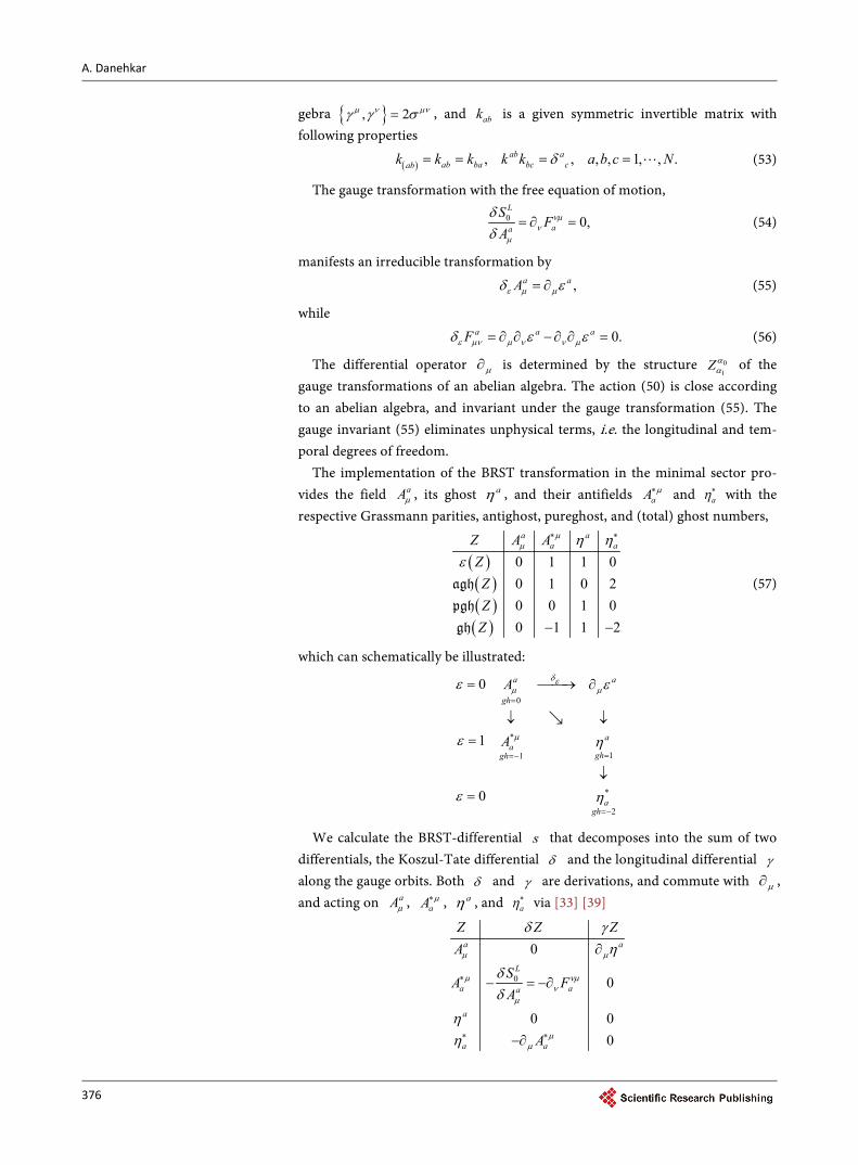
The implementation of the BRST transformation in the minimal sector pro-vides the field aAµ , its ghost aη , and their antifields aA µ∗ and aη

∗ with the respective Grassmann parities, antighost, pureghost, and (total) ghost numbers,

( )( )( )( )

0 1 1 00 1 0 20 0 1 00 1 1 2

a aa aZ A A

ZZZZ

µµ η η

ε

∗ ∗

− −

agh

pgh

gh

(57)

which can schematically be illustrated:

0

*

11

*

2

0

1

0

a a

gh

aa

ghgh

agh

A

A

δεµ µ

µ

ε ε

ε η

ε η

=

==−

=−

= → ∂

↓ ↓=

↓=

We calculate the BRST-differential s that decomposes into the sum of two differentials, the Koszul-Tate differential δ and the longitudinal differential γ along the gauge orbits. Both δ and γ are derivations, and commute with µ∂ , and acting on aAµ , aA µ∗ , aη , and aη

∗ via [33] [39]

0

0

0

0 00

a a

L

a aa

a

a a

Z Z ZA

SA F

A

A

µ µ

µ νµν

µ

µµ

δ γη

δδ

ηη

∗

∗ ∗

∂

− = −∂

−∂

A. Danehkar

377

The classical master Equation (47) of the action (50) holds the minimal solu-tion (45) in such a way

0 0 d .L a D aaS S A xA µ

µ µη∗ = + ∂ ∫

(58)

5.1. First-Order Deformation

We now consider the deformed solution of the master equation for the action (50) smoothly in the coupling constant λ that brings to the solution (58), while the coupling constant λ vanishes. In Section 4, we noticed that the first-order deformation ( 1λ ) of the master equation satisfies the solution 1 0sS = , where

1S is bosonic (commutative) function with ghost number zero. Let us assume

1 d ,DS xa= ∫ (59)

where a is a local function. Then, the first-order deformation, 1 0sS = , takes the local form

( )d 0D xsa sa a a jµµδ γ= → = + = ∂∫ (60)

( ) ( )0, 0,a aε= =gh (61)

where jµ is a local current that manifests the non-integrated density of the first-order deformation corresponding to the local cohomology of s in ghost number zero, ( )0a H s d∈ , where d is the exterior spacetime differential.

To evaluate Equation (60), we assume

( ) ( ) ( )0

, , 0, 0, 0, , ,I

i i i ii

a a a i a a i Iε=

= = = = ∀ =∑ agh gh

(62)

( )

( )( )

( )( )

( )( )

0, , 0, 0,

i i iiI

ij j j i j jµ µ µ µ µε

=

= = = =∑ agh gh

(63)

where ( )k

jµ are some local currents. Substituting (62) and (63) into (60) yields ( )

0 0 0,

iI I I

i ii i i

a a jµµδ γ= = =

+ = ∂∑ ∑ ∑

(64)

obviously

( ) ( )1, .i ia i a iδ γ= − =agh agh (65)

They can be decomposed on the several orders of the antighost number:

( )( )

( )

( )

1

1

1

,

1 ,

, 0, , 2

I

II

I Ik

k k

Z Z

I a j

I a a j

k a a j k I

µµ

µµ

µµ

γ

δ γ

δ γ

−

−

+

= ∂

− + = ∂

+ = ∂ = −

agh

(66)

The positive antighost number are strictly given as replacement for the first expression [35]:

A. Danehkar

378

( )0, 0 .II Ia I a Hγ γ= > → ∈ (67)

To proof it, let us consider Ie as the elements with pureghost number I of a basis in the polynomial space. The generic solution of (67) then takes the form

,II Ia eα= (68)

while

( ) ( ), .II I e Iα = =agh pgh

(69)

The objects Iα obviously are nontrivial in ( )0 ,H γ the so-called invariant polynomials. In other words, the strict positive antighost numbers provide tri-vially the cohomology of the exterior differential γ in the space of invariant polynomials Iα . Hence, a jµµγ = ∂ reduces to 0aγ = (see [35] for general proof).

Moreover, Ia may exclusively be reduced to γ -exact terms ,I Ia bγ= (70)

corresponding to a trivial definition, which states 0Ia = . This result is ob-viously given by the second-order nilpotency of γ that implies the unique so-lution of (67) up to γ -exact contributions, i.e.

,I I Ia a bγ→ + (71)

( ) ( ) ( ), 1, 1.I I Ib I b I bε= = − =agh pgh (72)

Hence, the non-triviality of the first-order deformation Ia requires the co-homology of the exterior longitudinal derivative γ in pureghost number equal to I , i.e. ( )I

Ia H γ∈ . To solve (66), it is necessary to provide the cohomology of γ and δ , ( )H γ and ( )H dδ :

( ) ,I I I Ia m a H dµµδ δ= ∂ → ∈

(73)

where

( ) ( ) , .IH d a a I a m Nµµδ δ= = = ∂agh

(74)

For an irreducible linear situation, where gauge generators are field indepen-dent, we assume that

( ) 0, 2.IH d Iδ = >

(75)

where ( )IH dδ manifests the local cohomology of the Koszul-Tate differential δ , while antighost number is I and pureghost number vanishes. In this case ( 2I = ), we obtain

( )

( )

21

2 10

1 0

0,

,

.

a

a a j

a a j

µµ

µµ

γ

δ γ

δ γ

= + = ∂ + = ∂

(76)

The first-order deformation up to antighost number two are:

0 1 2 .a a a a= + + (77)

The 2a is generated by arbitrarily smooth functions in the form (68), with

A. Danehkar

379

2α from ( )inv2H dδ and 2e denote the elements with pureghost number two

of a basis in the polynomial space, i.e.,

( ) ( ) ( )inv 22 2 2 2, 2,a H d eδ α∈ → = =agh pgh

(78)

where ( )invIH dδ is the local cohomology of the Koszul-Tate differential δ

with antighost number I in the invariant polynomial space. We now consider the Koszul-Tate differential δ and the exterior longitu-

dinal differential γ in the action (58):

0, , ,a aa a a aA A F Aµ νµ µ

µ ν µδ δη δ δη∗ ∗ ∗= = = −∂ = −∂

, 0.a aa aA Aα µ

µ µγ η γ γη γη∗ ∗= ∂ = = =

The local cohomology of the exterior longitudinal derivative γ in pureghost number one, ( )1 ,H γ has one ghost aη , while ( )2H γ has two ghosts a bη η , i.e.

( ) ( )1 2,a a bH Hη γ η η γ∈ ∈

(79)

From (79), we then solve

2 0,aγ =

by

21 ,2

a b ca bca fη η η∗=

(80)

where abcf contains the structure constants of a non-abelian algebra coupling

the Yang-Mills fields, and it is antisymmetric on indices bc :

[ ] .a a a abc bc cbbcf f f f= → = −

(81)

The expression ( )1

2 1a a jµµδ γ+ = ∂ is solved by taking the Koszul-Tate diffe-rential δ from (80):

( )

( ) ( )

212

12

a b ca bc

a b c a b ca bc a bc

a f

A f A f Aµ µµ µ

δ δ η η η

η η γ η

∗

∗ ∗

=

= − ∂ +

(82)

We simply notice that

( ) ( )21 .2

a b c a b ca bc a bca A f A A fµ µ

µ µδ γ η η η∗ ∗− = − ∂

(83)

This indicates ( )1

11, .2

a b c a b ca bc a bca A f A j A fµ µ µ

µη η η∗ ∗= − = −

(84)

To obtain 0a , we solve ( )0

1 0a a jµµδ γ+ = ∂ by taking the Koszul-Tate diffe-rential δ from 1a :

( )( )

1

1 1 .2 2

a b ca bc

a b c a b c a b ca bc a bc a bc

a A f A

F f A F f A A F f F

µµ

νµ νµ νµν µ ν µ νµ

δ δ η

η γ η

∗= −

= ∂ − + +

(85)

The last term in above relation vanishes, i.e.

A. Danehkar

380

0,a b ca bcF f Fνµ

νµη =

since 121 0,2

a b c m b a ca bc am bc

m b cmbc

F f F k F F f

F F f

νµ να µβνµ αβ νµ

να µβαβ νµ

η σ σ η

σ σ η

=

= =

while

, .ambc am bc mbc bmcf k f f f= = −

Therefore, we derive

( )11 .2

a b c a b ca bc a bca F f A A F f Aνµ νµ

ν µ ν µδ γ η − = ∂ −

(86)

It shows ( )0

01 , .2

a b c a b ca bc a bca F f A A j F f Aνµ µ νµ

ν µ µη= − = −

(87)

The results for the first-order deformation are summarized as follows:

1 1 .2 2

a b c a b c a b ca bc a bc a bca F f A A A f A fνµ µ

ν µ µη η η η∗ ∗= − − +

(88)

Finally, we derive

11 1d .2 2

D a b c a b c a b ca bc a bc a bcS x F f A A A f A fνµ µ

ν µ µη η η η∗ ∗ = − − + ∫

(89)

The first-order deformations of the solution ( 1S ) of the master equation were determined for the action (58). It is seen that gauge generators are field inde-pendent, and are reduced to a sum of terms with antighost numbers from zero to two.

5.2. Higher-Order Deformations

We now consider the higher-order deformations of the master equation for the action (50). The second-order deformation ( 2λ ) of the master equation are de-termined from the solution ( )1 1 2, 2 0S S sS+ = . Let us assume that

2 d ,DS xb= ∫ (90)

that takes the local form

2 .sb mµµ∆ + = ∂ (91)

Using the Equation (88) from Section 5.1, we calculate ( )1 1,S S :

( ) ( )( ) ( )( )

1 1, d d , d

d d , ,

D D D

D D

S S x xa ya

x y a x a x

≡ ∆ =

=

∫ ∫ ∫∫

while employing the following relations

( ) ( )( ) ( ) ( )( ) ( ), , ,a a a Db b bx y y x x yη η η η δ δ∗ ∗= = − −

(92)

( ) ( )( ) ( ) ( )( ) ( ), , ,a a a Db b bA x A y A y A x x yν ν ν

µ µ µδ δ δ∗ ∗= = − −

(93)

and the definitions

A. Danehkar

381

( ) ,g g gmg mgk f k A Aαρ βλ αρ βλ

ρλ ρ λ λ ρσ σ σ σ≡ ∂ − ∂

(94)

( ) ( ) ( )d .D Dx x y f x f yδ − ≡∫ (95)

They lead to the following expression ∆ :

( )( ) ( )

( ) ( )

a e m n p a e a e a e m n pem np a em np en pm ep mn a

a e a e m n p a m b c n pen pm em pn a bc ma np

a m b c n p a m b c n pbc ma np bc ma np

a mbc ma np

f f f f f f f f A A

f f f f F A A f k f A A A

f k f A A A f k f A A A

f k f

µµ

αβ αρ βµα β ρ µ α β

αρ βµ αµ βλρ µ α β λ µ α β

αµ

η η η η η η

η σ σ η

σ σ η σ σ η

σ σ

∗ ∗∆ = − − + +

+ − + ∂

+ ∂ − ∂

− ( ) ,b c n pA A Aβλρ µ α βη ∂

that is reduced to

[ ] [ ]

[ ] ( )

13!

2 .

a e m n p a e m n pa ae m np e m np

a e m n p a m b c n pa bc ma npe m np

f f f f A A

f f F A A f k f A A A

µµ

αβ αρ βµα β ρ µ α β

η η η η η η

η σ σ η

∗ ∗∆ = − −

− + ∂

We then decompose ∆ into the following terms,

0 1 2 ,∆ = ∆ + ∆ + ∆ (96)

namely,

[ ] ( )0 2 .a e m n p a m b c n pa bc ma npe m npf f F A A f k f A A Aαβ αρ βµ

α β ρ µ α βη σ σ η∆ ≡ − + ∂

(97)

[ ]1 ,a e m n pae m npf f A Aµ

µη η∗∆ ≡ −

(98)

[ ]21 ,3!

a e m n pae m npf f η η η η∗∆ ≡ −

(99)

We also define

0 1 2 .b b b b≡ + + (100)

From (91), it follows a set of equations ( )2

2 22 ,b mµµγ∆ + = ∂ (101)

( )1

1 2 12 2 ,b b mµµδ γ∆ + + = ∂ (102)

( )0

0 1 02 2 .b b mµµδ γ∆ + + = ∂ (103)

Equations (99) and (101) imply

2 20, 0,b∆ = = (104)

and

[ ] 0.a ee m npf f =

(105)

The later expression is called the Jacobi identity. Similarly, we obtain

1 10, 0.b∆ = = (106)

So, the Equation (103) remains to be solved:

( )( )0

02 2 .a m b c n pbc ma npf k f A A A b mαρ βµ µ

ρ µ α β µσ σ η γ∂ + = ∂

(107)

We solve it by substituting the exterior longitudinal differential γ of poten-

A. Danehkar

382

tials aAµ ( aA αµ µγ η= ∂ ):

( ) 12 .2

a m b c n p a m b c n pbc ma np bc am npf k f A A A f k f A A A Aαρ βµ αρ βµ

ρ µ α β ρ µ α βσ σ η γ σ σ ∂ = −

Accordingly, we derive

01 .4

a m b c n pbc am npb f k f A A A Aαρ βµ

ρ µ α βσ σ= −

Hence, the second-order deformations becomes

21d .4

D a m b c n pbc am npS x f k f A A A Aαρ βµ

ρ µ α βσ σ = − ∫

(108)

The Jacobi identity (105) obviously implies

( )1 2 3, 0 0.S S S= → =

Similarly, all deformations with orders higher than the second-order com-pletely vanish:

0, 3.kS k= ∀ ≥

As a result, the solution to the deformations becomes 20 1 2S S S Sλ λ= + + ,

that corresponds to the following Yang-Mills theory:

2

1d4

1 1 d2 21 d .4

D a aa a

D a b c a b c a b ca bc a bc a bc

D a m b c n pbc am np

S x F F A

x F f A A A f A f

x f k f A A A A

µν µµν µ

νµ µν µ µ

αρ βµρ µ α β

η

λ η η η η

λ σ σ

∗

∗ ∗

= − + ∂

+ − − + + −

∫

∫

∫

(109)

We have determined the Yang-Mills theory from the first- and second-order deformations of the master equation. The solutions of the master equation, which entirely include the gauge structures, are decomposed into terms with the antighost numbers from zero to two. In other words, the part with the antighost number equal to zero represents the Lagrangian action, while the antighost number one is proportional to the gauge generators. The terms with higher an-tighost numbers provide the reducibility functions, where the on-shell relations become linear components in the ghosts for ghosts. It is shown that all functions with order higher than second vanish in this model.

5.3. Interacting Theory

Let us consider the Equation (109) and identify the entire gauge structure of the Lagrangian model that describes all consistent interactions in the D-dimensional free Yang-Mills theory.

The antighost number zero of (109) shall provide the Lagrangian action of the interacting theory:

0

2

1 1d d4 2

1 d .4

L a D a D a b ca a bc v

D a m b c n pbc am np

S A x F F x F f A A

x f k f A A A A

µν νµµ µν µ

αρ βµρ µ α β

λ

λ σ σ

= − + − + −

∫ ∫

∫

(110)

A. Danehkar

383

Accordingly, the Yang-Mills theory is characterized by the following non- ab-elian action:

01d ,4

L a D aaS A x µν

µ µν = − ∫

(111)

where the non-abelian field strengths aµν is defined by

,a a a b cbcF f A Aµν µν µ νλ= + (112)

and abcf is the gauge-invariant that provides the gauge symmetry of the

Yang-Mills theory as follows

.a a a b c abcA f A Dε µ µ µ µδ ε λ ε ε= ∂ − ≡ (113)

So, the commutator among the deformed gauge transformations becomes:

1 2, .a aA Aε ε µ ε µδ δ δ =

(114)

The gauge symmetry remains abelian to order λ , and satisfies the equation of motion

0.aDµµν = (115)

The invariance of the action under the gauge transformations (113) is also obtained by the Noether identities

0 0.aaD D D

Aµ µ ν

µνµ

δδ

≡ =

(116)

The antighost number one of the deformation of the master equation allows to identify the gauge transformations (113) of the action (110) by substituting the ghost aη with gauge parameter aε . The antighost number two in (109) reads the complete gauge structure of the so-called interacting theory that de-termines the commutator (114) among the deformed gauge transformations.

6. Conclusion

In this paper, we reviewed deformed gauge transformations in the framework of the BRST-antifield formalism characterized by the antibracket that acts similar to the Poisson bracket in the Hamiltonian formalism. We provided the BRST cohomology of the consistent interactions through several order deformations of the master equation. The BRST-antifield formalism in the cohomological space provides the generalized framework of consistent interactions among fields with a gauge freedom by any types of invariant action. We see that higher order de-formations could be neglected due to non local interactions and their obstruction of consistent local couplings, which are associated with the anomalous gauge quantization. We demonstrated its functions by applying the BRST-antifield formalism to the D -dimensional, free Yang-Mills theory. All deformations of the master equation for the massless Yang-Mills model were calculated by using the cohomological groups ( ) , 0, , 2IH s d I = , of the BRST differential. The first-order deformation is provided by the cohomological group ( )1H s d , whereas the second-order deformation given by the cohomological group

A. Danehkar

384

( )2H s d obstructs all higher-order deformations. The results show that the deformations can be synthesized by the conception that all orders higher than two are trivial, while gauge generators are imposed to be field independent,

( ) 0, 2IH s d I= > . The deformations stopped at the second-order of the coupling constants characterize the consistent interactions, which maintain the equation of motion, and provide the entire gauge structure of the interacting Yang-Mills theory.

Acknowledgements

The author thanks the editor and the referee for their comments. Research of A. Danehkar is funded by the EU contract MRTN-CT-2004-005104. This support is greatly appreciated.

References [1] Dirac, P.A.M. (1950) Generalized Hamiltonian Dynamics. Canadian Journal of

Mathematics, 2, 129-148. https://doi.org/10.4153/CJM-1950-012-1

[2] Dirac, P.A.M. (1958) The Theory of Gravitation in Hamiltonian Form. Proceedings of the Royal Society A Mathematical, Physical and Engineering Sciences, London, 246, 333-343. https://doi.org/10.1098/rspa.1958.0142

[3] Dirac, P. (1964) Lectures on Quantum Mechanics. Yeshiva University, New York.

[4] Anderson, J.L. and Bergmann, P.G. (1951) Constraints in Covariant Field Theories. Physical Review, 83, 1018-1025. https://doi.org/10.1103/PhysRev.83.1018

[5] Bergmann, P.G. and Goldberg, I. (1955) Dirac Bracket Transformations in Phase Space. Physical Review, 98, 531-538. https://doi.org/10.1103/PhysRev.98.531

[6] Weinberg, S. (1995) The Quantum Theory of Fields. Cambridge University Press, Cambridge. https://doi.org/10.1017/CBO9781139644167

[7] Gotay, M.J. and Nester, J.M. (1979) Presymplectic Lagrangian Systems. I: The Con-straint Algorithm and the Equivalence Theorem. Annales de l’Institut Henri Poin-caré, 30, 129-142.

[8] Gotay, M.J. and Nester, J.M. (1980) Presymplectic Lagrangian Systems. II: The Se- cond-Order Equation Problem. Annales de l’Institut Henri Poincaré, 32, 1-13.

[9] Batlle, C., Gomis, J., Pons, J.M. and Roman-Roy, N. (1986) Equivalence between the Lagrangian and Hamiltonian Formalism for Constrained Systems. Journal of Ma-thematical Physics, 27, 2953-2962. https://doi.org/10.1063/1.527274

[10] Gitman, D.M. and Tyutin, I.V. (1990) Quantization of Fields with Constraints. Springer-Verlag, Berlin. https://doi.org/10.1007/978-3-642-83938-2

[11] Govaerts, J. (1991) Hamiltonian Quantisation and Constrained Dynamics. Leuven University Press, Leuven.

[12] Hanson, A., Regge, T. and Teitelboim, C. (1976) Constrained Hamiltonian Systems. Accademia Nazionale dei Lincei, Rome.

[13] Landau, L.D. and Lifshitz, E.M. (1976) Mechanics. Sykes, J.B. and Bell, J.S., Trans., Cambridge University Press, Cambridge.

[14] Sudarshan, E.C.G. and Mukunda, N. (1974) Classical Dynamics. Wiley, New York.

[15] Sundermeyer, K. (1982) Constrained Dynamics. Lecture Notes in Physics, Springer, Berlin.

[16] Becchi, C., Rouet, A. and Stora, R. (1974) The Abelian Higgs Kibble Model, Unitar-

A. Danehkar

385

ity of the S-Operator. Physics Letters B, 52, 344-346. https://doi.org/10.1016/0370-2693(74)90058-6

[17] Becchi, C., Rouet, A. and Stora, R. (1975) Renormalization of the Abelian Higgs- Kibble Model. Communications in Mathematical Physics, 42, 127-162. https://doi.org/10.1007/BF01614158

[18] Becchi, C., Rouet, A. and Stora, R. (1976) Renormalization of Gauge Theories. An-nals of Physics, 98, 287-321. https://doi.org/10.1016/0003-4916(76)90156-1

[19] Tyutin, I.V. (1975) Gauge Invariance in Field Theory and Statistical Physics in Op-erator Formalism. LEBEDEV-75-39. arXiv:0812.0580 [hep-th]

[20] Brandt, F., Dragon, N. and Kreuzer, M. (1989) All Consistent Yang-Mills Anoma-lies. Physics Letters B, 231, 263-270. https://doi.org/10.1016/0370-2693(89)90211-6

[21] Brandt, F., Dragon, N. and Kreuzer, M. (1989) All Solutions of the Consistency Eq-uations. DESY 89-076, ITP-UH 2/89.

[22] Fisch, J., Henneaux, M., Stasheff, J. and Teitelboim, C. (1989) Existence, Uniqueness and Cohomology of the Classical BRST Charge with Ghosts of Ghosts. Communi-cations in Mathematical Physics, 120, 379-407. https://doi.org/10.1007/BF01225504

[23] Henneaux, M. (1990) Lectures on the Antifield-BRST Formalism for Gauge Theo-ries. Nuclear Physics B—Proceedings Supplements, 18, 47-105. https://doi.org/10.1016/0920-5632(90)90647-D

[24] Batalin, I.A. and Vilkovisky, G.A. (1981) Gauge Algebra and Quantization. Physics Letters B, 102, 27-31. https://doi.org/10.1016/0370-2693(81)90205-7

[25] Batalin, I.A. and Vilkovisky, G.A. (1983) Quantization of Gauge Theories with Li-nearly Dependent Generators. Physical Review D, 28, 2567-2582. https://doi.org/10.1103/PhysRevD.28.2567

[26] Batalin, I.A. and Vilkovisky, G.A. (1984) Erratum: Quantization of Gauge Theories with Linearly Dependent Generators. Physical Review D, 30, 508. https://doi.org/10.1103/PhysRevD.30.508

[27] Fisch, J.M.L. and Henneaux, M. (1990) Homological Perturbation Theory and the Algebraic Structure of the Antifield-Antibracket Formalism for Gauge Theories. Communications in Mathematical Physics, 128, 627-640. https://doi.org/10.1007/BF02096877

[28] Henneaux, M. and Teitelboim, C. (1991) Quantization of Gauge Systems. Princeton University Press, Princeton.

[29] Gomis, J. and Paŕis, J. (1993) Field-Antifield Formalism for Anomalous Gauge Theories. Nuclear Physics B, 395, 288-324. hep-th/9204065 https://doi.org/10.1016/0550-3213(93)90218-E

[30] Gomis, J., Pars, J. and Samuel, S. (1995) Antibracket, Antifields and Gauge-Theory Quantization. Physics Reports, 259, 1-145. hep-th/9412228 https://doi.org/10.1016/0370-1573(94)00112-G

[31] Barnich, G. and Henneaux, M. (1993) Consistent Couplings between Fields with a Gauge Freedom and Deformations of the Master Equation. Physics Letters B, 311, 123-129. hep-th/9304057 https://doi.org/10.1016/0370-2693(93)90544-R

[32] Henneaux, M. (1998) Consistent Interactions between Gauge Fields: The Cohomo-logical Approach. Contemporary Mathematics, 219, 93-109. hep-th/9712226 https://doi.org/10.1090/conm/219/03070

[33] Barnich, G., Brandt, F. and Henneaux, M. (1995) Local BRST Cohomology in the Antifield Formalism: II. Application to Yang-Mills theory. Communications in Mathematical Physics, 174, 93-116. hep-th/9405194 https://doi.org/10.1007/BF02099465

A. Danehkar

386

[34] Bizdadea, C. (2000) On the Cohomological Derivation of Topological Yang-Mills Theory. Europhysics Letters, 52, 123-129. hep-th/0006218 https://doi.org/10.1209/epl/i2000-00413-7

[35] Cioroianu, E.M. and Sararu, S.C. (2005) Self-Interactions in a Topological BF-Type Model in D=5. Journal of High Energy Physics, 2005, JHEP07. hep-th/0508035 https://doi.org/10.1088/1126-6708/2005/07/056

[36] Bizdadea, C., Cioroianu, E.M., Danehkar, A., Iordache, M., Saliu, S.O. and Sararu, S.C. (2009) Consistent Interactions of Dual Linearized Gravity in D=5: Couplings with a Topological BF Model. European Physical Journal C, 63, 491-519. arXiv:hep-th/0908.2169 https://doi.org/10.1140/epjc/s10052-009-1105-0

[37] Barnich, G., Henneaux, M. and Tatar, R. (1994) Consistent Interactions between Gauge Fields and Local BRST Cohomology: The Example of Yang-Mills Models. International Journal of Modern Physics D, 3, 139-144. hep-th/9307155 https://doi.org/10.1142/S0218271894000149

[38] Bizdadea, C., Ciobirca, C.C., Cioroianu, E.M., Saliu, S.O. and Sararu, S.C. (2003) Hamiltonian BRST Deformation of a Class of N-Dimensional BF-Type Theories. Journal of High Energy Physics, 2003, JHEP01. hep-th/0302037 https://doi.org/10.1088/1126-6708/2003/01/049

[39] Barnich, G., Brandt, F. and Henneaux, M. (2000) Local BRST Cohomology in Gauge Theories. Physics Reports, 338, 439-569. hep-th/0002245 https://doi.org/10.1016/S0370-1573(00)00049-1

A. Danehkar

387

Appendix Antibracket Structure

For a function ( )X ψ in a generic space, commutative or anticommutative, we state:

, .l rX XX Xψ ψ ψ ψ

∂ ∂∂ ∂= =

∂ ∂ ∂ ∂

(117)

The left derivative l∂ is an ordinary derivative (left to right). The right de-rivative r∂ is the derivative action from right to left.

For any ( )X ψ in a generic space, we get

( ) ( )11 .Xl rX Xψε ε

ψ ψ+∂ ∂

= −∂ ∂

(118)

Considering Equation (32) and Equation (118), it follows that

( ) ( )( )( ) ( )1 1, 1 , .X YX Y Y Xε ε+ += − −

Assuming X Y= , one can find

( )( )( )1 11 .X Xl lr rA A

A A

X XX Xε ε+ +

∗ ∗

∂ ∂∂ ∂= −

∂Φ ∂Φ ∂Φ ∂Φ (119)

For bosonic (commutative) and fermionic (anticommutative) variables, we have

( )2 is commutative,

,0 is anticommutative.

lrA

A

XX XX X

X

∗

∂∂ ∂Φ ∂Φ=

(120)

For any X , we have

( )( ), , 0, .X X X X= ∀

(121)

Furthermore, the antibracket has the following properties:

( ) ( ) ( ) ( ), , 1 , ,Y ZX YZ X Y Z X Z Yε ε= + − (122)

( ) ( ) ( ) ( ), , 1 , ,X YXY Z X Y Z Y X Zε ε= + − (123)

( )( ) ( )( )( ) ( )( ) ( )( )( ) ( )( )1 1, , 1 , , 1 , , 0.X Y Z Z X YX Y Z Y Z X Z X Yε ε ε ε ε ε+ + + ++ − + − = (124)

Submit or recommend next manuscript to SCIRP and we will provide best service for you:

Accepting pre-submission inquiries through Email, Facebook, LinkedIn, Twitter, etc. A wide selection of journals (inclusive of 9 subjects, more than 200 journals) Providing 24-hour high-quality service User-friendly online submission system Fair and swift peer-review system Efficient typesetting and proofreading procedure Display of the result of downloads and visits, as well as the number of cited articles Maximum dissemination of your research work

Submit your manuscript at: http://papersubmission.scirp.org/ Or contact jhepgc@scirp.org