on the center-of-mass free density matrix - progress of theoretical

414

Progress of Theoretical Physics, Vol. 76, No.2, August 1986

On the Center-of-Mass Free Density Matrix

Kazuhiro Y ABANA

Department of Physics, Kyoto University, Kyoto 606

(Received January 7, 1986)

Two methods to calculate the density matrix of one· body or more·than·one·body which does not include the spurious center·of·mass excitation are presented. One is the method to calculate the density matrix for the many-body wave function of general type and the other is applicable to the case in which the center~of-mass motion separates from the internal motion and is in the (Os) orbit of harmonic oscillator. The applications of these methods are illustrated for some many-body wave function.

§ 1. Introduction

To represent the characteristic features of the many-body wave function of nuclei, the density matrices are often utilized. Experimentally, for example, in the electron scattering from nuclei, the nuclear structure is analyzed by the terms of the nuclear density and the current density, which are the special forms of the one-body density matrix. Theoretically, the one-body density matrix plays a crucial role in the current nuclear theories based on the mean field approximation, such as Hartree-Fock theory. And, in recent nuclear studies, interest is taken in not only the nuclear density which is the diagonal part of the one-body density matrix, but the non-local part of it. The non-local part of the one-body density matrix is often visualized with the use of the Wigner transform of it. 1

),2)

Especially, in the time-dependent Hartree-Fock theory, the Wigner transform of the one-body density matrix is interpreted as the classical distribution function and obeys the Vlasov equation approximately.3) These works clarify the importance of the non-local part of the one-body density matrix in the dynamics.

Usually the spatial coordinate of the density matrix is measured from some spatially fixed origin. Due to the finiteness of the nuclear system, however, we need to measure the coordinate from the center of mass of the system; otherwise the spurious center-of-mass motion affects the density matrix. This effect of center-of-mass motion becomes important for light systems. For the diagonal part of the one-body transition density matrix, the effect of center-of-mass motion was discussed by Tassie and Barker for the case of harmonic oscillator shell mode1. 4

) And for the diagonal part of the one-body density matrix in momentum representation, that is the nuclear momentum distribution, the effect of spurious center-of-mass motion has been discussed. 5

) For the general non-local density matrix, however, there seems not to be presented any method to treat the spurious center-of-mass effect.

In this paper, we present two methods to get the center-of-mass free density matrix. One is the method, applicable to the general wave function, which is especially suitable for the case where the wave function is a (linear superposition of) Slater determinant. The other is applicable to the cases in which the center-of-mass motion separates from other internal motions and is in the (Os) orbit of harmonic oscillator. For such wave functions, the latter method is more easy to calculate though the former method is also applicable.

The construction of this paper is as follows: In § 2, we present some preparations for

Dow

nloaded from https://academ

ic.oup.com/ptp/article/76/2/414/1848559 by guest on 29 D

ecember 2021

On the Center-of Mass Free Density Matrix 415

later discussion; the notations of the coordinate systems are introduced, and the center-ofmass free density matrix is defined. In § 3, we present a method to calculate the center-ofmass free one-body and more-than-one-body density matrices for the general many-body wave function. In § 4, another method to calculate the center-of-mass free density matrix is presented, which is applicable to the cases where the center-of-mass motion separates from the internal motion and is in the (Os) orbit of harmonic oscillator. In § 5, some applications of these methods are discussed and the summary is presented in § 6.

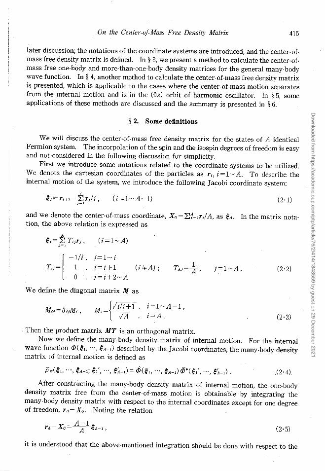
§ 2. . Some definitions

We will discuss the center-of-mass free density matrix for the states of A identical Fermion system. The incorpolation of the spin and the isospin degrees of freedom is easy and not considered in the following discussion for simplicity.

First we introduce some notations related to the coordinate systems to be utilized. We denote the cartesian coordinates of the particles as ri, i = 1 ~ A. To describe the internal motion of the system, we introduce the following Jacobi coordinate system:

(2'1)

and we denote the center-of-mass coordinate, XC=L:1=lrJA, as ~A. In the matrix notation, the above relation is expressed as

j

-1Ii' j=l~i

Tij = 01, j = i + 1 (i * A) ; , j=i+2~A

We define the diagonal matrix M as

Mi = {! il i + 1, i = 1 ~ A-I , IA , i=A.

Then the product matrix MT is an orthogonal matrix.

(2· 2)

(2' 3)

Now we define the many-body density matrix of internal motion. For the internal wave function iP(~l, "', ~A-l) described by the Jacobi coordinates, the many-body density matrix of internal motion is defined as

(2'4)

After constructing the many-body density matrix of internal motion, the one-body density matrix free from the center-of-mass motion is obtainable by integrating the many-body density matrix with respect to the internal coordinates except for one degree of freedom, r A - Xc. Noting the relation

(2' 5)

it is understood that the above-mentioned integration should be done with respect to the

Dow



ecember 2021

416 K. Yabana

Jacobi coordinates ~1 ~ ~A-2. Thus we are led to the following formula for the center-ofmass free one-body density matrix p.p(l)(a, a ' ):

(1)( ') -A( A )3 - (o( A A ') p.p a, a - A-I p.p A -1 a, A -1 a , (2·6)

(2'7)

where we have introduced the one-body densitY,matrixp.p(l)(a, a' ) with respect to the Jacobi coordinate ~A-1. The numerical factor A(A/ A -1)3 in Eq. (2'6) assures the usual normalization of the one-body density matrix, Jdap.p(l)(a, a) =A, for the normalized wave function (/).

Expressions similar to Eq. (2'6) for the center-of-mass free density matrix of morethan-one-body are obtainable in the following way. To get the nobody center-of-mass free density matrix, we need to integrate the many-body density matrix of Eq. (2·4) over the internal coordinates except for n-degrees of freedom, (r A-n+l - X G) ~ (r A - X G). For this purpose we invert the coordinate transformation of Eq. (2·2) as

(2·8)

where the second equality is due to the fact that the product matrix MT is orthogonal. Because the matrix element Tji equal to zero for j< i-I, Eq. (2'8) shows that ri-~A is expressible with the Jacobi coordinates ~i-l ~ ~A-1. From the above consideration, the coordinates (rA-n+1- X G) ~ (rA - X G) are expressible by the Jacobi coordinates ~A-n~ ~A-1, and the integrations of the remaining degrees of freedom should be achieved with respect to the Jacobi coordinates ~1 ~ ~A-n-1. Therefore the center-of-mass free nobody density matrix is obtainable from the following nobody density matrix with respect to the Jacobi coordinates:

= fd~1···d~A-n-1p.p(~1'-··' ~A-n-1, aA-n, "', aA-1; ~1, "', ~A-n-1, a~-n, "', a~-l) . (2'9)

From p.p(n), the nobody density matrix with respect to the cartesian coordinates, ri- XG(i =A-n+l~A), is obtainable by inverting the relation of Eq. (2'8). For the two-body case, for example, we get

(2'10)

From the above relations, the center-of-mass free two-body density matrix p.p(2)(a, b; a',

b' ) for the cartesian coordinates rA-1- XG and rA - XG is expressed as

Dow



ecember 2021

___ .J

On the Center-afMass Free Density Matrix

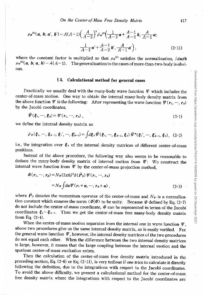
(2)( b ' b') A(A 1)( A )3 -- (2)( 1 + A-I b A . PIP a, ; a , = - A - 2 PIP A - 2 a A - 2 'A -1 a,

1 '+ A-I b' A - ,) A-2 a A-2 'A-l a ,

417

(2·11)

where the constant factor is multiplied so that PIP(2) satisfies the normalization, f dadb PIP(2)(a, b; a, b) =A(A -1). The generalization to the cases of more-than-two-body is obvious.

§ 3. Calculational method for general cases

Practically we usually deal with the many-body wave function lJf which includes the center-of-mass motion. One way to obtain the internal many-body density matrix from the above function lJf is the following: After representing the wave function lJf (rl, ... , r A) by the Jacobi coordinates,

(3·1)

we define the internal density matrix as

i.e., the integration over ~A of the internal density matrices of different center-of-mass positions.

Instead of the above procedure, the following way also seems to be reasonable to deduce the many-body density matrix of internal motion from lJf: We construct the internal wave function from lJf by the center-of-mass projection method,

<P(rl, ... , r1) = N7Jf(27rh) 30 CPG) lJf(rl, .•• , rA)

(3·3)

where PG denotes the momentum operator of the center-of-mass and N7Jf is a normalization constant which ensures the norm <<PI<p) to be unity. Because <P defined by Eq. (2·7) do not include the center-of-mass coordinate, <P can be represented in terms of the Jacobi coordinates ~l ~ ~A-l. Then we get the center-of-mass free many-body density matrix from Eq. (2·4).

When the center-of-mass motion separates from the internal one in wave function lJf, above two procedures give us the same internal density matrix, as is easily verified. For the general wave function qr, however, the internal density matrices of the two procedures do not equal each other. When the difference between the two internal density matrices is large, however, it means that the large coupling between the internal motion and the spurious center-of-mass excitation exists.

Then the calculation of the center-of-mass free density matrix introduced in the preceding section, Eq. (2·6) or Eq. (2·11), is very tedious if one tries to calculate it directly following the definition, due to the integrations with respect to the Jacobi coordinates. To avoid the above difficulty, we present a calculational method for the center-of-mass free density matrix where the integrations with respect to the Jacobi coordinates are

Dow



ecember 2021

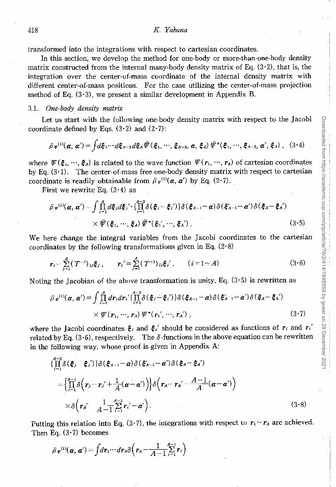
418 K. Yabana

transformed into the integrations with respect to cartesian coordinates. In this section, we develop the method for one-body or more-than-one-body density

matrix constructed from the internal many-body density matrix of Eq. (3·2), that is, the integration over the center-of-mass coordinate of the internal density matrix with different center-of-mass positions. For the .case utilizing the center-of-mass projection method of Eq. (3·3), we present a similar development in Appendix B.

3.1. One-body density matrix

Let us start with the following one-body density matrix with respect to the Jacobi coordinate defined by Eqs. (3·2) and (2·7):

pw(1)(a, a')= fd~I"'d~A-2d~Aljf(~I' "', ~A-2, a, ~A) ljf*(~I, "', ~A-2, a', ~A), (3·4)

where lfI"(~I, "', ~A) is related to the wave function lfI"(rl, "', rA) of cartesian coordinates by Eq. (3·1). The center-of-mass free one-body density matrix with respect to cartesian coordinate is readily obtainable from p w(l)(a, a') by Eq. (2·7). .

First we rewrite Eq. (3·4) as

(3· 5)

We here change the integral variables from the Jacobi coordinates to the cartesian coordinates by the following transformations given in Eq. (2·8)

(3·6)

Noting the Jacobian of the above transformation is unity, Eq. (3·5) is rewritten as

(3· 7)

where the Jacobi coordinates ~i and ~/ should be considered as functions of ri and r/ related by Eq. (3·6), respectively. The (3 -functions in the above equation can be rewritten in the following way, whose proof is given in Appendix A:

( 1 A-I )

X(3 r/- A-I ~Ir/-a' . (3·8)

Putting this relation into Eq. (3·7), the integrations with respect to rl~rA are achieved. Then Eq. (3·7) becomes

Dow



ecember 2021


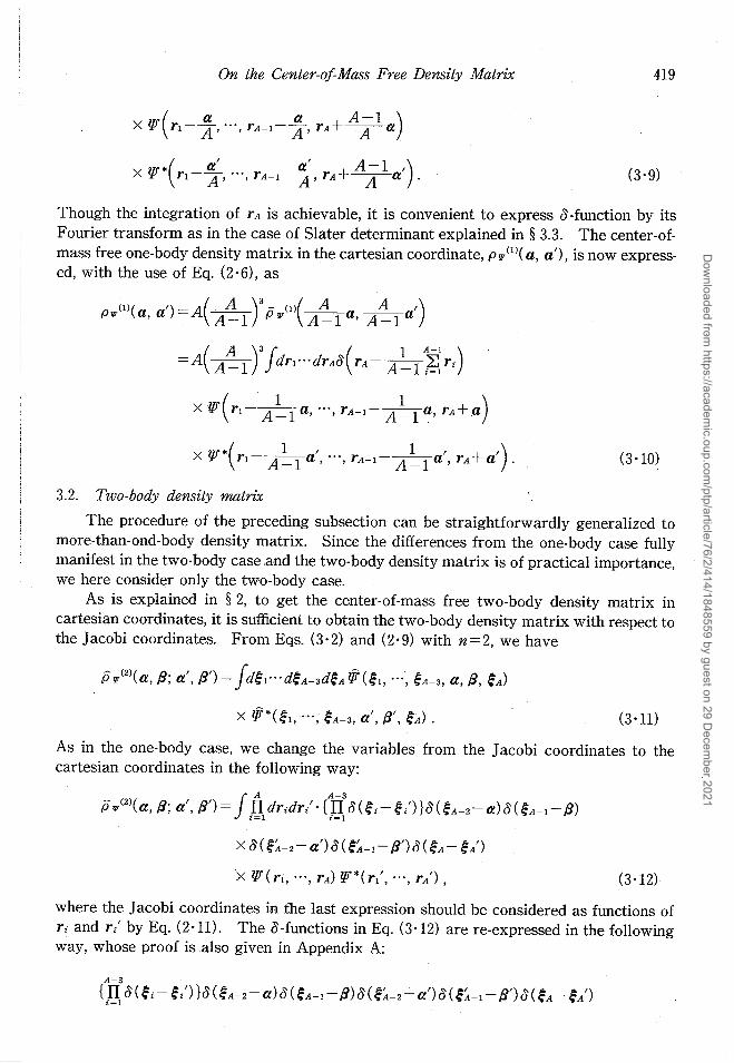
(3·9)

Though the integration of rA is achievable, it is convenient to express ·a-function by its Fourier transform as in the case of Slater determinant explained in § 3.3. The center-ofmass free one-body density matrix in the cartesian coordinate, pqr(I)( a, a'), is now expressed, with the use of Eq. (2·6), as

(1)( ')_A(~)3- (I)(~ ~,) pqr a, a - A-I pqr A-I a, A-I a

(3 ·10)

3.2. Two-body density matrix

The procedure of the preceding subsection can be straightforwardly generalized to more-than-ond-body density matrix. Since the differences from the one-body case fully manifest in the two-body case and the two-body density matrix is of practical importance, we here consider only the two-body case.

As is explained in § 2, to get the center-of-mass free two-body density matrix in cartesian coordinates, it is sufficient to obtain the two-body density matrix with respect to the Jacobi coordinates. From Eqs. (3·2) and (2·9) with n=2, we have

if qr(2)(a, P; a', P') = fd~I···d~A-3d~A ljf(~I, ... , ~A-3, a, p, ~A)

(3·11)

As in the one-body case, we change the variables from the Jacobi coordinates to the cartesian coordinates in the following way:

fA A-3

if qr(2)(a, P; a', P') = II dridr;'· {g a (~i- ~;') }a( ~A-2- a) a (~A-l - P)

x a(~~-2-a')a(~~-I- P')a(~A- ~A')

(3 ·12)

where the Jacobi coordinates in fhe last expression should be considered as functions of ri and r;' by Eq. (2·11). The a-functions in Eq. (3·12) are re-expressed in the following way, whose proof is also given in Appendix A:

Dow



ecember 2021

420 K. Yabana

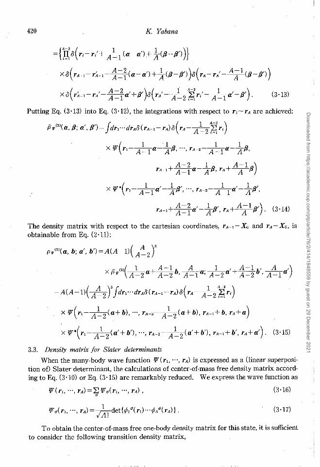
{A-2 ( 1 1)} = ll18 ri- r/ + A-I (a-a') +jf(P-P')

x 8( rA-l- r~-1-1 =i (a-a') + ~ (P-P') )8(rA- r/ - A Al (P-P'»)

(3·13)

Putting Eq. (3·13) into Eq. (3·12), the integrations with respect to rl ~ rA are achieved:

(3·14)

The density matrix with respect to the cartesian coordinates, rA-l- XG and rA - XG, is obtainable from Eq. (2·11):

P'l'(2)(a, b; a', b')=A(A-1)(A~2r

- (2)( 1 + A-I b A . 1 , + A -1 b' A ,) x P'I' A - 2 a A - 2 'A -1 a, A - 2 a A - 2 'A -1 a

=A(A -1)( A ~2 r !dr1"'drA8(rA- 1- rA)o( rA - A ~2 :~: ri)

x lJf(rl- A~2(a+b), "', rA-2- A~2(a+b), rA-l+b, rA+a)

X lJf*(r1- A~2(a'+b')' "', rA-2- A~2(a'+b')' rA-l+b', rA+a'). (3·15)

3.3. Density matrix for Slater determinants

When the many-body wave function lJf(rl, "', rA) is expressed as a (linear superposition of) Slater determinant, the calculations of center-of-mass free density matrix according to Eq. (3 ·10) or Eq. (3 ·15) are remarkably reduced. We express the wave function as

(3·16)

(3·17)

To obtain the center-of-mass free one-body density matrix for this state, it is sufficient to consider the following transition density matrix,

Dow



ecember 2021


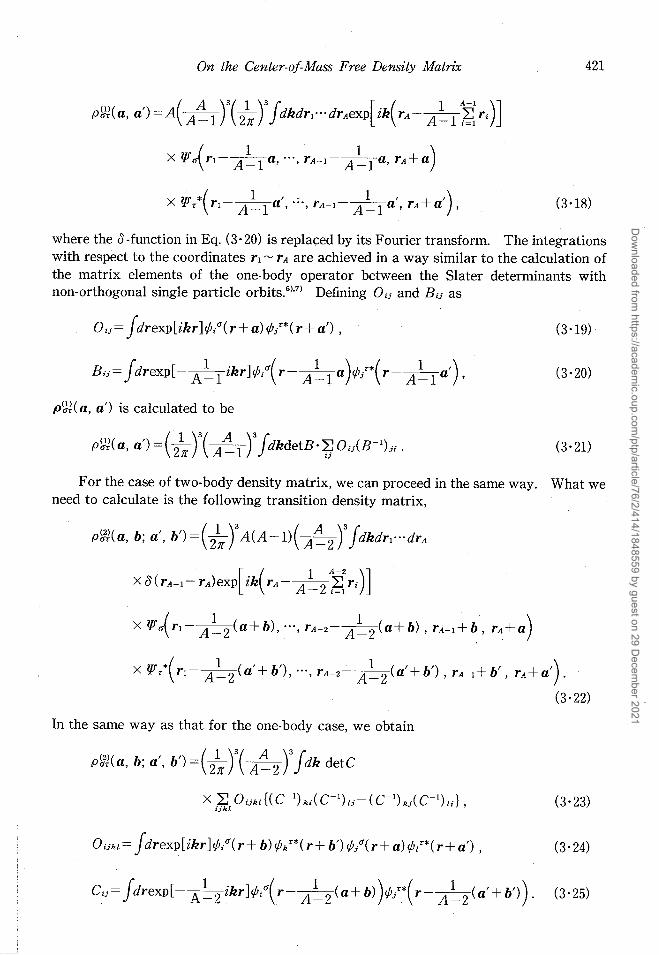
(3·18)

where the 0 -function in Eq. (3·20) is replaced by its Fourier transform. The integrations with respect to the coordinates r1 ~ 1"A are achieved in a way similar to the calculation of the matrix elements of the one-body operator between the Slater determinants with non-orthogonal single particle orbits. 6

),7) Defining Oij and Bij as

Oij= jdrexp[ikr ]¢/( r+ a) ¢/*( r+ a') , (3 ·19)

Bij= jdrexp[- A~l ikr]¢/{r- A~l a)¢r(r- A~l a')' (3·20)

p<,}f( a, a') is calculated to be

(3· 21)

For the case of two-body density matrix, we can proceed in the same way. What we need to calculate is the following transition density matrix,

XlJfo{r1- A~2(a+b), ... ,rA-2- A~2(a+b),rA-1+b, rA+a)

X lJf/(r1- A~2(a'+b'), "', rA-2- A~2(a'+b')' rA-1+b', rA+a').

(3·22)

In the same way as that for the one-body case, we obtain

p<Jl(a, b; a', b')=(2~r(A~2rjdk detC

x ~ Oijkl{(C-1)ki(C-1)lj-(C-1)kj(C-1)li} , (3·23) ijkl

Dow



ecember 2021

422 K. Yabana

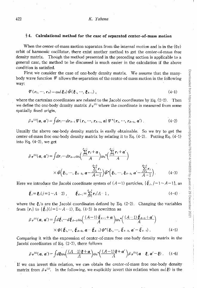
§ 4. Calculational method for the case of separated center-of-mass motion

When the center-of-mass motion separates from the internal motion and is in the (Os) orbit of harmonic oscillator, there exist another method to get the center-of-mass free density matrix. Though the method presented in the preceding section is applicable to a general case, the method to be discussed is much easier in the calculation if the above condition is satisfied.

First we consider the case of one-body density matrix. We assume that the manybody wave function 1fJ' allows the separation of the center-of-mass motion in the following way:

(4 ·1)

where the cartesian coordinates are related to the Jacobi coordinates by Eq. (2·2). Then we define the one-body density matrix j5 w(!) where the coordinate is measured from some spatially fixed origin,

(4· 2)

Usually the above one-body density matrix is easily obtainable. So we try to get the center-of-mass free one-body density matrix by relating it to Eq. (4·2). Putting Eq. (4 ·1) into Eq. (4·2), we get

A-I A-I . ~~ ~~)

x @( ~I, "', ~A-2, a- A~ 1 )@*( ~I, "', ~A-2, a' - A~ 1 . (4· 3)

Here we introduce the Jacobi coordinate system of (A -1) particles, {fj, j= 1 ~ A -I}, as

_ A-I ~A-I= ~ rJA-l, (4·4)

i=l

where the ~/s are the Jacobi coordinates defined by Eq. (2·2). Changing the variables from {ri} to {fi}(i=I~A-l), Eq. (4·3) is rewritten as

- (1)( ') _ {d£: "'d£: ( (A-I) fA-I + a) *( (A -1) fA-I + a') Pw a,a-j''i l 'iA-I(()O A (()o A

Comparing it with the expression of center-of-mass free one-body density matrix in the Jacobi coordinates of Eq. (2· 7), there follows

- (1)( ')- (dl: ((A-l)~+a) *((A-l)~+a')_ (1)( -I: a'-I:) (4.6) P w a, a - ) I 'i(()O A (()o A P w a 'i, 'i.

If we can invert this relation, we can obtain the center-of-mass free one-body density matrix from j5w(l). In the following, we explicitly invert this relation when (()o(~) is the

Dow



ecember 2021

___ -.-1

On the Center-afMass Free Density Matrix 423

Gaussian function,

( 2Av )3/4

wo(~)= ------;r exp{-Ave}. (4· 7)

After putting Eq. (4·7) into Eq. (4·6), we change the variables from a, a' to r, s as

a+a' r=--2-'

, s=a-a ,

and change ~-+ - ~+ r. Then Eq. (4·6) becomes

- (1)( s -~)-J. (2Av)3/2 [_ (A-1)2{ _~ }2_~ 2J P'l' r+Z ' r 2 - d~ 7f exp 2v A ~ A -1 r 2A s

x - (1)( e+~ e_~) P'l' ,. 2'" 2 .

(4· 8)

(4·9)

Now the r-dependence on the right-hand side is only through the Gaussian function. So we can easily invert Eq. (4·9), which results in

- (l)(e+~ e_~)_(_1 )3(A-:-1)3 (~2) P 'l' ,. 2 ,,. 2 - 27f A exp 2A s

- (1)( + s s) XP'l' r Z' r-Z . (4·10)

The change of variables from t s to a, a' by the same relation as Eq. (4·8) gives us the desired expression for P'l'(1)(a, a'). The center-of-mass free one-body density matrix with respect to the cartesian coordinate is obtained with the use of Eq. (2·6):

(1)( ')_A(~)3- (l)(~ ~,) P'l' a, a - A-1 P'l' A-1 a, A-1 a

_ ( 1 )3 [v ( A)2 , 2J - 2i[ Aexp 2A A-1 (a-a)

x - (1)( A . A , ) P'l' A-1 a-r, A-1 a -r . (4 ·11)

The generalization to the more-than-one-body case is straightforward. We consider the two-body case for illustration. As in the one-body case, we introduce the two-body density matrix,

which is assumed to be already obtained. It can be related to the center-of-mass free two-body density matrix in the same way as that of the one-body case,

Dow



ecember 2021

424 K. Yabana

p7[l(2)(a, b; a', b') = fd~Wo( (A -2)~+a+ b )wo*( (A -2)~+ a' + b')

x - (2)( e, b 1 A - 2 e, , e, b' 1 ,A - 2 e,) P7[l a- .. , - A-I a- A-I"; a - .. , - A-I a - A-I" . (4-13)

When the center-of-mass wave function is given by Eq. (4-7), we get the following expression for the center-of-mass free two-body density matrix by inverting Eq. (4-13),

(2)( b. ' b')-A(A-1)(~)3 - (2)(_1_ + A-I b ~ . P7[I a, ,a, - A-2 P7[I A-2 a A-2 'A-1 a,

1 '+ A-I b' A ') A-2 a A-2 'A-1 a

( 1 )3 [J,V ( A )2( a + b

= 2J[ A(A -l)exp ff\ A -2 2

R+ 1 '+ A-I b' R+ A ') A-2 a A-2' A-I a . (4 -14)

§ 5_ Application to some shell model wave functions

As examples of the application of the method to calculate the center-of-mass free density matrix, we present the calculations of center-of-mass free one-body density matrix. for some shell model wave functions for some doubly closed shell nuclei.

First we consider the harmonic oscillator shell model wave function for ground state and take the 160 nucleus for illustration. The wave function is given by

( 2v )3/4

cpop,( r) = 2/V n (eir )exp( - vr2) , (i=x,y,Z) (5-1)

where ei denotes the unit vector for i-direction. As is well known, the center-of-mass motion separates from the internal motion in the harmonic oscillator shell model without particle-hole excitations:

(5- 2)

So we can apply the method presented in § 4. The one-body density matrix measured from the spatially fixed origin is given by

Dow



ecember 2021


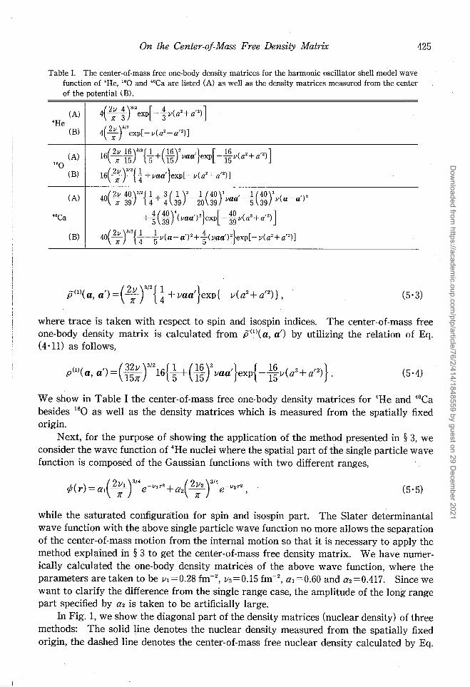
Table I. The center-of-mass free one-body density matrices for the harmonic oscillator shell model wave function of 4He, 160 and 40Ca are listed (A) as well as the density matrices measured from the center of the potential (B).

(Zv 4 r [ 4 ] (A) 4 7r3 exp -3v(a2+ a'2) 4He

(2vr (B) 47r exp[-v(a2+a'2)]

(Zv 16 r {I (16 r '} [ 16 2 '2 ] (A) 16 7r15 s+ 15 vaa exp -15v(a +a ) 160

(Zvre } (B) 16 7r · 4+ vaa' exp[-v(a2+a'2)]

(A) ( 2v 40 r {I t( 1 r to{ 40), , 1 ( 40), , 2 4° 7r39 4+ 4 39 - 20 39 vaa -S 39 v(a-a)

40Ca + i(~~r(vaa')2}exp[ -~~v(a2+a'2)J

(B) (Zvre 1 4} 40 7r 4-Sv(a-a')2+S(vaa')2 exp[ - v(a2+a'2)]

(5-3)

where trace is taken with respect to spin and isospin indices. The center-of-mass free one-body density matrix is calculated from p(l)(a, a') by utilizing the relation of Eq. (4 -11) as follows,

(1)( ') _(~)3/216{l+(li)2 '} {_li ( 2+ '2)} P a, a - 15IT 5 15 1/aa exp 151/ a a . (5-4)

We show in Table I the center-of-mass free one-body density matrices for 4He and 40Ca besides 160 as well as the density matrices which is measured from the spatially fixed origin.

Next, for the purpose of showing the application of the method presented in § 3, we consider the wave function of 4He nuclei where the spatial part of the single particle wave function is composed of the Gaussian functions with two different ranges,

¢( ) _ (21/1 )3/4 -Vl r2 + (21/2 )3/4 -lJ2r2 r - al IT e a2 IT e , (5-5)

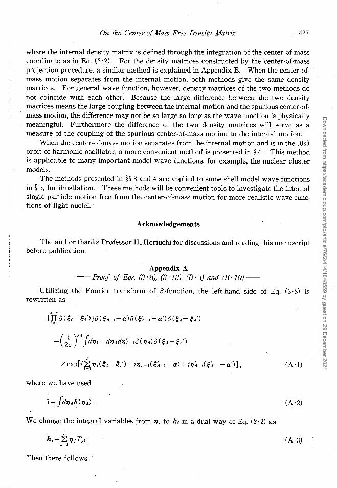
while the saturated configuration for spin and isospin part. The Slater determinantal wave function with the above single particle wave function no more allows the separation of the center-of-mass motion from the internal motion so that it is necessary to apply the method explained in § 3 to get the center-of-mass free density matrix. We have numerically calculated the one-body density matrices of the above wave function, where the parameters are taken to be 1/1 =0.28 fm-2, 1/2=0.15 fm-2, al =0.60 and a2=0.417. Since we want to clarify the difference from the single range case, the amplitude of the long range part specified by a2 is taken to be artificially large.

In Fig. 1, we show the diagonal part of the density matrices (nuclear density) of three methods: The solid line denotes the nuclear density measured from the spatially fixed origin, the dashed line denotes the center-of-mass free nuclear density calculated by Eq.

Dow



ecember 2021

426 K. Yabana

P(o,a)

0.3

0,2

0,1

o 2 3 a (fm)

Fig. 1. The diagonal part of the one· body density matrices (nuclear density) for 4He nuclei with the spatial wave function of Eq. (5·5). Solid line denotes the nuclear density measured from the spatially fixed origin, dashed line the center-ofmass free nuclear density obtained by the integration with respect to center-of-mass coordinate and dash-dotted line the center-of-mass free nuclear density for the center-of-mass projected wave function.

02 1(0,0') lo+o'I=2fm

0,1

o 2 3 " 5 6 la-a'i (fm)

Fig. 2. The non-local part of the one-body density matrices, where la+a'I=2fm,la-a'l is to be varied, while a + a' and a - a' are set to be orthogonal to each other. The three lines correspond respectively to those in Fig. 1.

(3 ·10), that is, the integration of the center-of-mass free density matrices with different center-of-mass coordinates, and the dash-dotted line denotes the center-of-mass free nuclear density for the projected wave function calculated by Eq. (B·5)_ Figure 2 shows the non-local part of the one-body density matrices where la+ a'i =2fm and la- a'i is to be varied, while two vectors, a+ a' and a- a', are taken to be orthogonal to each other. The three lines represent the same as that in Fig. 1. The difference between the center-ofmass free density matrices of two different methods is very small so that it can be said the coupling between the spurious center-of-mass excitation and the internal motion is very small in this wave function.

§ 6. Summary

In this paper, we have developed a method to calculate the center-of-mass free density matrix, which enables us to get the non-local part of the density matrix as well as the local part. The method is quite convenient when the many-body wave function is described by a (linear superposition of) Slater determinant.

Thecenter-of-mass free one-body or more-than-one-body density matrices with respect to cartesian coordinates are introduced in § 2, relating it to the density matrices with respect to the Jacobi coordinates.

In § 3,a calculational method for the center-of-mass free density matrices is presented,

Dow



ecember 2021


where the internal density matrix is defined through the integration of the center-of-mass coordinate as in Eq. (3·2). For the density matrices constructed by the center-of-mass projection procedure, a similar method is explained in Appendix B. When the center-ofmass motion separates from the internal motion, both methods give the same density matrices. For general wave function, however, density matrices of the two methods do not coincide with each other: Because the large difference between the two density matrices means the large coupling between the internal motion and the spurious center-ofmass motion, the difference may not be so large so long as the wave function is physically meaningful. Furthermore the difference of the two density matrices will serve as a measure of the coupling of the spurious center-of-mass motion to the internal motion.

When the center-of-mass motion separates from the internal motion and is in the (Os) orbit of harmonic oscillator, a more convenient method is presented in § 4. This method is applicable to many important model wave functions, for example, the nuclear cluster models.

The methods presented in §§ 3 and 4 are applied to some shell model wave functions in § 5, for illustlation. These methods will be convenient tools to investigate the internal single particle motion free from the center-of-mass motion for more realistic wave functions of light nuclei.

Acknowledgements

The author thanks Professor H .. Horiuchi for discussions and reading this manuscript before publication.

Appendix A - Proof of Eqs. (3, 8), (3 '13), (B, 3)' and (B '10)-

Utilizing the Fourier transform of a-function, the left-hand side of Eq. (3'8) is rewritten as

A

X exp[i ~ TJ;( ~i- ~;') + iTJA-l (~~-l- a) + iTJ~-I(~~-I- a')] , z=l

(A'l)

where we have used

(A·2)

We change the integral variables from TJi to hi in a dual way of Eq. (2·2) as

(A'3)

Then there follows '

Dow



ecember 2021

428 K. Yabana

A-I 1 A-I 7)A-I=-A kA--A ~ki~kA, :=1

(A-4)

where the indication by arrow is due to 0 (7)A) in Eq. (A -1). Noting that the Jacobian of the transformation, Eq. (A-3), is unity, Eq. (A-I) becomes

(A -I) =( 2~ yA fdkI···dkAd7)~-IO(7)A)O(~A - ~A') A

X exp[i ~ k;( r;- r;') + ikA(~~-I - a) + i7)~-I( ~~-I- a')] . i=l

(A-5)

After expressing 0 ( 7) A) as

(A-6)

integrations with respect to kI ~ kA and 7)~-I are achieved, which results in

(A-I) = fdsttt o(r;- r;' +s) }o(rA - rA' +s-a+a')o(~~-I-a')o(~A - ~A') .

(A-7)

Utilizing the o-functions of Eq. (A-7), ~A-~A' is expressed as

~ -s+ } (a-a') . (A-8)

Integration with respect to s gives us just the right-hand side of Eq. (3-8) if we express ~~-I as rA'-~1':-lr//A-1.

Equation (3 -13) is shown in a similar way. The left-hand side of Eq. (3 -13) is rewritten, in the same way as Eq. (A -1), as

A

xexp[i ~ 7);(~i- ~;') + i7)A-2(~~-2- a) + i7)A-I( ~~-I-13) i=l

+ i7)~-2( ~~-2 - a') + i7)~-I (~~-I - 13')] . (A-g)

Then we change 7)i into k i through Eq. (A-3). Noting Eq. (A-4) and

(A-I0)

where indication by arrow is the same that in Eq. (A-4), Eq. (A-g) is written as

Dow



ecember 2021

J

On the Center-of Mass Free Density Matrix

(A·9) =(2~ rA+I)fdkl ... dkAdkA~ldkA' O(7)A)O(~A- ~/)

xexp[ i tl kj(rj- r/) + i( A ~ 1 kA + kA-I )(~A-2-a) + ikA(~A-I- fJ)

+ i( A ~ 1 k/ + kA-I )(~A-2-a') + ik/(~A-I- fJ)] ,

where the following transformation is done,

(7):-2)= (1 1/ (A -l))(kA~I) . 7)A-I 0 1 kA

429

(A·n)

(A ·12)

Putting Eq. (A· 6) into Eq. (A ·n), the integrations with respect to kl' ... , kA, kA-I and kA' are achieved, which results in

(A·9) = fd8("'f1 o(r;- r/ +8) }o(rA-l- r~-I-(a-a') +8)

X o( rA - rA' - A ~ 1 (a-a') -(fJ-fJ') +8 )o( r~-I- r/ -1 =i a' +fJ')

xo(rA'- A~2 ~:r/- A~1 a'-fJ')o(~A-~/)' (A·13)

where ~A-2 and ~A-I are replaced by r~-I- L!1,;:-lr/ /A -2 and r/ - L!1,;:-fr/ /A -1, respectively. Utilizing the o-functions of Eq. (A· 13), ~A-~A' is re-expressed as

(A· 14)

Then the integration of 8 is achieved, which just gives us the right-hand side of Eq. (3·13). The left-hand sides of Eqs. (B· 3) and (B ·10) are just the left-hand side of Eqs. (3·8)

and (3·13) if we remove O(~A-~A'), respectively. So we can obtain Eqs. (B ·4) and (B·n) by removing O(~A-~/) in Eqs. (A·7) and (A·13), respectively.

Appendix B

We here derive the formulas for center-of-mass free density matrices of the internal many-body wave function constructed by the center-of-mass projection method.

B.I. One-body density matrix

Consider the one-body density matrix with respect to the Jacobi coordinate defined by Eq. (2·7). Putting Eq. (2·4) into Eq. (2·7), we get

p w(l)(a, a') = fd~I···d~A-2(jj(~I' ... , ~A-2, a) (jj*(~I, ... , ~A-2, a')

Dow



ecember 2021

430 K. Yabana

(B·!)

where, in the last equality, the transformation of Eq. (3'6) is made and ~i, ~/ in the last expression should be considered as functions of ri, r/, respectively. f/J(rl, "', rA) is related to rJj(~I, .. ·, ~A-I) by the coordinate transformation of ri and ~i. We here assume that the wave function f/J( rl, "', rA) is constructed from 1Jf (rl, "', rA) by the center-of-mass projec-

. tion method of Eq. (3'3). Putting Eq. (3'3) into Eq. (E'1), there follows

( A A-2 P 7[I(1)(a, a') =N7[l2J dudu'Dldridr/' {lI 8(~i- ~/)}

x 8 (~A-I- a) 8( ~~-I- a') 8(~A) 8( ~A')

fA A-2

=N 7[12 II dridr;'· {lI 8(~i- ~/) }8(~A-I- a)8(~~-I- a')

(B·2)

The 8 -functions in the above expression can be re-expressed in the following way as is shown in Appendix A:

{ A-I ( 1 A-I ) = J ds {DI8(ri-r/+s)}8(rA-r/+s-a+a')8 r/- A-I ~Ir/-a' . (B'3)

Putting it into Eq. (B'2), the integrations with respect to rl ~ rA are achieved,

x 1Jf(rl, "', rA-I, rA+a) 1Jf*(rl+s, "', rA-I+s, rA+s+a'). (B·4)

The one-body density matrix with respect to the cartesian coordinate is obtained from Eq. (2'6) as

(1)( ') _ A(~)3 - (1)(~ ~,) P7[l a, a - A -1 P 7[1 A -1 a, A -1 a

x 1Jf*(rl+s, "', rA-I+s, rA+s+ A~l a'). (B·5)

When the wave function is a (linear superposition of) Slater determinant as Eqs. (3·16) and (3 ,17), we obtain the following expression in the same way as in § 3.3:

Dow



ecember 2021

----~

On the Center-ai-Mass Free Density Matrix

=(Zl7[ Y(A~lyNw2jdsdk det B'~OdB-Ih,

Bij= jdrexp[- A~l ikr]¢/(r)¢/*(r+s) ,

Oij= jdrexP[ikr]¢/(r+ A~l a)¢/*(r+s+ A~l a').

B.Z. Two-body density matrix

431

(B·6)

(B·?)

(B·S)

For the internal wave function constructed by the center-of-mass projection method, the two-body density matrix with respect to the Jacobi coordinates ~A-2 and ~A-I is expressed, in the same way of Eqs. (B·1) and (B·Z) for one-body case, as

j A A-3

P w(2)(a, /3; a', /3') =Nw2 llJridr/' {iII O(~i- ~/) }O(~A-2-a)o(~A-I-/3)

XO(~~-2-a')o(~~-I-/3') 1J!(rl, ... , rA) 1J!*(rl', ... , rA'). (B'9)

The 0 -functions of the above expression is re-expressed, as shown in Appendix A, in the following way,

= jds(ri o(ri- r/ +s) }o(rA-I- r~-l +s-(a-a'))

x o( rA- rA' +s- A ~ 1 (a-a') -(/3-/3'))

(B·10)

Putting Eq. (B·10) into Eq. (B'9), the integrations with respect to rl ~ rA are achieved. We get the following expression,

p w(2)(a, /3; a', /3') =Nw2 jdsdrl···drAo(rA-1- rA)o( rA- A ~Z ~: ri)

x 1J!*(rl+s, ... , rA-2+s, rA-I+s+a', rA+s+ A~l a'+/3').

(B. 11)

The two-body density matrix with respect to the cartesian coordinates, rA-I- XG and rA-XG , is obtained, utilizing the relation of Eq. (Z·l1):

(2)( b. ' b')-A(A-1)(~)3 - (2)(_1_ + A-I b ~ . p w a, ,a, - A _ 2 p w A - 2 a A - 2 'A _ 1 a,

Dow



ecember 2021

432 K. Yabana

1 '+ A-I b' A ,) A-2 a A-2 'A-l a

( 1 A-I A-II)

x1Jf rl, ... , rA-2, rA-I+ A-2 a+ A-2 b, rA+ A-2 a+ A-2 b

x 1Jf*( rl +s, ... , rA-2+s, rA-I +S+ A ~2 a' + 1 =~ b',

+ + A-I '+ 1 b') rA S A-2 a A-2 .

When the wave function is a (linear superposition of) Slater determinant as Eqs. (3·16) and (3·17), we obtain the following expression for the transition two-body density matrix:

( 1 A-I A-II)

x 1Jf15 rl, ... , rA-2, rA-I+ A-2 a+ A-2 b, rA+ A-2 a+ A-2 b

x 1Jfr*(rl+S, ... , rA-2+s, rA-I+s+ A~2 a'+ 1=~ b',

+ + A-I '+ 1 b') rA S A-2 a A-2

Cij= !drexp[ - A~2 ikr]¢/(r)¢/*(r+s) ,

(B·13)

(B·14)

Oijkl= !drexp[ikr ]¢/(r+ A~2 a+ 1=~ b )¢kT*(r+s+ A~2 a'+ 1=~ b')

(B·15)

References

1) G. F. Bertsch, "Many-Body Dynamics of Heavy-Ion Collisions", in Les Houches Lecture Notes, ed. R. Balian et a!. (North-Holland, Amsterdam, 1978), p. 178.

2) J. Martorell and E. Moya de Guerra, Ann. of Phys. 158 (1984), 1. M. Prakash, S. Shlomo and V. M. Kolomiety, Nuc!. Phys. A370 (1981), 30.

3) M. Prakash, S. Shlomo, B. S. Nilsson, J. P. Bondorf and F. E. Serr, Nuc!. Phys. A385 (1982), 483. H. S. Kohler and H. Flocard, Nuc!. Phys. A323 (1979), 189.

4) L. J. Tassie and F. C. Barker, Phys. Rev. 111 (1958), 940. 5) For example, J. G. Zabolitzky and W. Ey, Phys. Lett. 76B (1978), 527. 6) D. M. Brink, Proc. Int. School of Phys., Enrico Fermi 36 (Academic Press, 1966), 247. 7) H. Horiuchi, Prog. Theor. Phys. Supp!. No. 62 (1977), 90.

Dow



ecember 2021

on the center-of-mass free density matrix - progress of theoretical

Documents