on the calibration of the sabr–libor market model correlations · model of interest forward rates...
TRANSCRIPT

On the Calibration of the
SABR–Libor Market Model Correlations
Master’s Thesis
Dr. Elidon Dhamo
Christ Church College
University of Oxford
Submitted in Partial Fulfillment for the MSc in
Mathematical Finance
September 2011


To Migena ...

Abstract
This work is concerned with the SABR-LMM model. This is a term structuremodel of interest forward rates with stochastic volatility that is a naturalextension of both, the LIBOR market model (Brace-Gatarek-Musiela [1997])and the SABR stochastic volatility model of Hagan et al. [2002].
While the seminal approximation formula (developed by Hagan et al. [2002])to implied Black volatility using the SABR model parameters allows fora successful calibration of each forward rate dynamics to the volatilitysmile of the respective caplets/floorlets, an adequate calibration of the richcorrelation structure of SABR-LMM (correlations among the forward rates,the volatilities and the cross correlations) is a challenging topic and of greatinterest in practice. Although widely used for calibration, it is well knownthat swaptions’ volatilities carry only little information about correlationsamong the forward rates. As practically successful for the classical LMM,desirable would be to take the market swap rate correlations into account forthe model calibration.
In this study we develop a new approach of calibrating the model correlations,aiming at incorporating the market information about the forward rate corre-lations implied from more correlation-sensitive products such as CMS spreadderivatives, in which also swap rate correlations are involved. To this end wederive a displaced-diffusion model for the swap rate spreads with a SABRstochastic volatility. This we achieve by applying the Markovian projectiontechnique which approximates the dynamics of the basket of forward rates, interms of the terminal distribution, by a univariate displaced-diffusion. TheCMS spread derivatives can then be priced using the SABR formulas for theimplied volatility, taking the whole market smile of CMS spread options intoconsideration. For the ATM values in the payoff measure of the projectedSDE we use a standard smile-consistent replication of the necessary convexityadjustment with swaptions.
Numerical simulations conclude the work, giving a comparison between thismethod and the classical one of calibrating the model correlations to swaptionvolatilities. Furthermore, we study the performance of different parameteriza-tions of the correlation (sub-)matrices.
v


Acknowledgements
First of all, I would like to thank Dr. Christoph Reisinger for agreeing tosupervise this thesis, his support and his encouragements.
I would like to express my gratitude towards my former employer, d-fineGmbH, for offering me the opportunity to take part in the MathematicalFinance course at the University of Oxford, and for providing financial support.
Last but not least I am particularly indebted to my family for their understand-ing, their great moral support and their patience over the numerous weekendsI did not spend with them.
vii


Contents
Introduction 1
Chapter 1. Forward Libor and Swap Market Models 4
1.1 A Review of the Classical Libor and Swap Market Models . . . . . . 4
1.1.1 Libor Dynamics Under the Forward Measure . . . . . . . . . . 7
1.1.2 Valuation in LMM . . . . . . . . . . . . . . . . . . . . . . . . 8
1.1.3 Covariance and Correlations in LMM . . . . . . . . . . . . . . 9
1.1.4 Swap Rate Models and Measures . . . . . . . . . . . . . . . . 10
1.1.5 Incompatibility Between the LMM and the SMM . . . . . . . 11
1.2 The Convexity Adjustment and CMS Derivatives . . . . . . . . . . . 13
1.2.1 Constant Maturity Swaps and Related Derivatives . . . . . . . 14
1.2.2 Valuation of CMS Derivatives . . . . . . . . . . . . . . . . . . 16
1.3 Parameterization and Calibration . . . . . . . . . . . . . . . . . . . . 22
1.3.1 Parametric Forms of the Instantaneous Volatilities . . . . . . . 23
1.3.2 Calibration to the Cap/Floor Market . . . . . . . . . . . . . . 24
1.3.3 The Structure of Instantaneous Correlations . . . . . . . . . . 25
1.3.4 Calibration of LMM Correlations to Swaptions Volatilities . . 30
1.3.5 Calibration to Correlations Implied From CMS Spread Options 30
Chapter 2. The SABR Model of Forward Rates 32
2.1 General Model Dynamics . . . . . . . . . . . . . . . . . . . . . . . . . 32
2.1.1 The Time-Homogeneous Model . . . . . . . . . . . . . . . . . 34
2.1.2 Joint Dynamics of the SABR Forward Rates and Their Volatilities 35
2.2 Valuation in the SABR Model . . . . . . . . . . . . . . . . . . . . . . 36
Chapter 3. Pricing CMS Derivatives in SABR 37
3.1 The Markovian Projection Method . . . . . . . . . . . . . . . . . . . 37
3.2 A Displaced SABR Diffusion Model for CMS Derivatives . . . . . . . 38
3.2.1 Projection of CMS-Spreads to Displaced SABR Diffusion . . . 38
ix

Contents x
3.2.2 Pricing of CMS-Spread Options in a SABR Displaced DiffusionModel . . . . . . . . . . . . . . . . . . . . . . . . . . . . . . . 45
Chapter 4. The SABR-LMM Model and Its Calibration 48
4.1 SABR–Consistent Extension of the LMM and Its Calibration . . . . . 48
4.2 Calibrating the Volatility Process . . . . . . . . . . . . . . . . . . . . 50
4.3 The SABR Correlation Structure . . . . . . . . . . . . . . . . . . . . 51
4.4 Calibration of the SABR–LMMCorrelations to Swaption Implied Volatil-ities . . . . . . . . . . . . . . . . . . . . . . . . . . . . . . . . . . . . 52
4.5 Calibrating to Correlations Implied From CMS Spread Options . . . 55
4.6 Numerical Simulations . . . . . . . . . . . . . . . . . . . . . . . . . . 56
Chapter 5. Conclusion and Outlook 59
Appendix A. Classical Models and SABR-LMM 60
A.1 Valuation in LMM . . . . . . . . . . . . . . . . . . . . . . . . . . . . 60
A.2 Swap Rate Dynamics and the Choice of Numeraire . . . . . . . . . . 63
A.3 Valuation in the Log-Normal Swap Market Model . . . . . . . . . . . 64
A.4 Drift Approximation in LMM and Simulations . . . . . . . . . . . . . 65
A.5 SABR Implied Volatility . . . . . . . . . . . . . . . . . . . . . . . . . 66
Appendix B. Calibration Details 69
B.1 Bootstrapping the Market Data . . . . . . . . . . . . . . . . . . . . . 69
B.2 Parameterization of SABR–LMM and Its Calibration . . . . . . . . . 71
B.2.1 Parameterization of the SABR–LMM Model . . . . . . . . . . 71
B.2.2 Calibration Procedure . . . . . . . . . . . . . . . . . . . . . . 72
Bibliography 77

Introduction
While the Brace-Gatarek-Musiela (BGM) or Libor1 Market Model (LMM), based onthe assumption that forward term rates follow lognormal processes under their cor-responding forward measure, has established itself as a benchmark model for pricinginterest rate derivatives, it is less successful in recovering other essential characteris-tics of interest rate markets, particularly volatility skews and smiles. The presenceof these volatility skew and smiles in the market, however, indicates that a purelognormal forward rate dynamics is not appropriate.
In the last decade several extensions of the BGM model have been proposed, inwhich various versions of the volatility structures of forward Libor rates have beendesigned to match the observed volatility smile effects in the market. The set ofextensions covers local volatility, jump-diffusion and stochastic volatility models withand without time-dependent parameters. The calibration procedures in most of thesemodels are complicated and computationally expensive, and are performed on a best-fit basis.
One of the most successful and popular extensions of the LMM, the SABR2 model,models the forward rate process under its forward measure using a correlated log-normal stochastic volatility process. Its success is indebted to two main propertiesof the model: the crucial property of taking into account the quality of prediction ofthe future dynamics of the volatility smile, meeting the observations from the marketreality, and the seminal asymptotic expansion formula, developed by Hagan et al.[2002], to approximate the implied Black volatility using the SABR model parame-ters. Hence, prices of options, such as caps and floors, can be calculated using thewell known Black pricing framework but taking the volatility smile surface via theSABR parameters into account.
The SABR model and the LMM, although modeling the same assets, ”do not directlytalk to each other”3. The SABR does not link the snapshots of the caplet smiles intowell-defined joint dynamics. To overcome this Rebonato [2007] introduced a naturalextension of the LMM, the SABR-LMM, that recovers the SABR caplet prices almostexactly for all strikes and maturities. The dynamics of the volatility in this model ischosen so as to be consistent across expiries and to make the evolution of the impliedvolatilities as time-homogeneous as possible.
While the approximation to implied Black volatility using the SABR model parame-ters allows for a successful calibration of each forward rate dynamics to the volatility
1Libor = London Inter-Bank Offered Rates2Launched by Hagan et al. [2002]3Rebonato [2007]
1

Introduction 2
smile of the respective caplets and floorlets, an adequate calibration of the rich cor-relation structure of SABR-LMM (comprising correlations among the forward rates,the volatilities and the cross correlations) is a challenging topic and of great inter-est in practice. Although widely used for calibration, it is well known that swap-tion volatilities carry only little information about correlations among the forwardrates4. Facing the richness of the correlation structure of SABR-LMM, the needfor a calibration approach to more correlation-sensitive products is obvious and ofwide practical interest. As already successfully applied for the classical LMM5, it isdesirable to additionally take the swap rate correlations into account for the modelcalibration, which consistently are to be implied from the market prices of appropri-ate products. A broadly known and traded class of interest rate derivatives meetingthese requirements, particularly incorporating information about the swap rate cor-relations, is the one of Constant Maturity Swap (CMS) spread derivatives. Whilevaluation (in all the mentioned forward rate models) of these products is typicallydone straight-forwardly by Monte-Carlo simulation, the calibration of the models tothese products, by finding accurate and fast analytical approximations to reproducethe prices of these instruments, has been always subject to research6, even within thesimpler LMM framework7.
Scope of the Present Work and Contribution
In this work we develop a novel approach for the calibration of the rich correlationstructure in the SABR-LMM model of forward rates. Given the reasons above, ourscope is to extract the information about the forward rate correlations from themarket prices of correlation-sensitive derivatives, such as CMS spread options, andfit the model correlation parameters to those. To this end the derivation of analyticalpricing formulas for these products in the SABR framework is necessary.
The Markovian projection (MP) technique8 is an effective technique to volatilitycalibration that seeks to optimally approximate a complex underlying process witha simpler one, keeping essential properties of the initial process, and is, in principle,applicable to any diffusion model.
Starting with the SABR-LMM we apply the MP technique to the CMS spreads andderive a displaced–diffusion SABR model for the spread between the swap rates withdifferent maturities. To achieve this we adapt the recent work of Kienitz-Wittkey[2010], carried out in a SABR swap rate framework, to our SABR-LMM model.Consequently, we can price the CMS spread options in the resulting SABR swapspread model by making use of the seminal SABR formula of Hagan et al. [2002]. Inthis way we can calibrate the SABR swap spread model parameters to the marketimplied (normal) volatilities of the corresponding CMS spread options. For the ATM
4We refer at this point to the works of Alexander [2003], Brigo-Mercurio [2007], Rebonato[2002], Schoenmakers [2002, 2005], Schoenmakers-Coffey [2003].
5Borger-van Heys [2010].6Antonov-Arneguy [2009], Castagna-Mercurio-Tarenghi [2007], Lutz [2010], Kienitz-Wittkey
[2010], etc.7Belomestny-Kolodko-Schoenmakers [2010], Borger-van Heys [2010], etc.8MP has been introduced in this context by Piterbarg [2003, 2005a,b] and formalized in Piterbarg
[2007].

Introduction 3
values in the expiry forward measure of the projected SDE (i.e. expiry time of thecorresponding CMS spread option) we use a standard smile-consistent replication9 ofthe necessary convexity adjustment with swaptions. By this means we shall be able toimplicitly retrieve the important information about swap rate correlations containedin the market smile of CMS spread options and embed it into the SABR-LMM modelcorrelations.
This work is concluded with the numerical implementation of this new calibrationprocedure and some numerical simulations. We shall discuss different parameteri-zations of the sub-matrices of the model correlation matrix, in particular the Doustparameterizations, and study the performance of this calibration approach, in termsof pricing errors for swaptions, in comparison to the approach of calibrating the modelcorrelations to swaptions’ implied volatilities, given in Rebonato [2007].
The performed simulations shall also illustrate the effectiveness and robustness ofthis approach, and provide information about expected and possible drawbacks.
Outline
The thesis is organized as follows.
In the first chapter we review the classical forward LIBOR and swap rate marketmodels. Particular focus is set on the introduction of convexity and the differentapproaches to carry out the convexity correction. We incorporate these methods tothe pricing of CMS derivatives, in particular, the CMS caps and spread options. Wealso describe the calibration of LMM and introduce the different parameterizationsof the correlation matrix. At the end of the chapter a recent approach to implycorrelations from CMS spread options is presented.
The second chapter is devoted to introduction and general properties of the SABRmodel.
The application of the Markovian Projection (MP) method to the basket of forwardrates is carried out in the third chapter. Here we derive a displaced-diffusion modelfor the swap rate spread with a SABR stochastic volatility. For the pricing of CMSspread caplets in the payoff forward measure we use a smile-consistent replication ofthe convexity adjustment for the ATM spreads via swaptions, and apply the Haganet al. [2002] formulae.
The SABR-LMMmodel is introduced in the fourth chapter which is mainly concernedwith the parameterization and the calibration of the model. Two different approachesto correlation calibration are presented. Numerical simulations give a comparisonbetween the these approaches, taking different parameterizations of the sub-matricesof the correlation matrix into account.
We conclude the work by presenting a short summary of our analysis, and give anoutlook of possible future directions of the discussed topics.
9According to Hagan [2003].

Chapter 1
Forward Libor andSwap Market Models
1.1 A Review of the Classical Libor and Swap
Market Models
Over the past two decades the Brace-Gatarek-Musiela [1997] model (BGM) has es-tablished itself as a benchmark model for pricing and risk managing interest ratederivatives. It is based on the assumption that the forward rates follow lognormalprocesses with deterministic (time-dependent) volatilities under their correspond-ing measures, and it is widely known as the lognormal forward Libor Market Model(LMM). The popularity of this model is indebted to its compatibility with the seminalBlack model which establishes a direct relationship between caplets’ prices and local(implied) volatilities of forward rates and constitutes the standard market conventionfor quoting benchmark instruments.
While the LMM model has established a standard for incorporating all available at-the-money information, it is less successful in recovering other essential characteristicsof interest rate markets, particularly volatility skews and smiles1. Various extensionsof the LMM model, designed to incorporate skew and smile effects, have been pro-posed. The set of extensions covers local volatility, jump-diffusion and stochasticvolatility models with and without time-dependent parameters. In the next chap-ters we shall discuss one of the most successful extensions of the LMM, the SABRmodel, which enjoys increasing popularity among the practitioners and academicsalike, again due to its compatibility with the Black ’s framework.
Nevertheless, one of the biggest challenges in using these models is the calibrationof the forward rate correlations which are not covered by the caplets markets, butrather incorporated in other benchmark instruments, such as European swaptionsor CMS spread derivatives. While the valuation in all these forward rate models is
1The volatility tends to rise if the option is out of the money. This results in the so calledvolatility smile describing the fact that implied Black volatility is strike-dependent.
4

Chapter 1. Forward Libor and Swap Market Models 5
typically done straight-forwardly by Monte-Carlo simulation, calibration by findingaccurate and fast analytical approximations to prices of these benchmark instrumentshas always been subject to research.
In this chapter we briefly describe the construction of forward Libor models as givenin Brace-Gatarek-Musiela [1997] and Jamshidian [1997], whereby we follow theapproach proposed by Musiela-Rutkowski [2005]. Assuming, for the time being,that there are no smile effects present in the interest rate markets, the formal modelsetup we present here is based on assumptions made in Musiela-Rutkowski [2005].In the following sections we shall present some of the mostly used parameterizationsand calibration methods for the forward rate volatilities and their correlations, whichwill prepare the ground for introducing the SABR-LMM model in the next chaptersand its calibration approaches. We shall also briefly mention the lognormal swaprate model (SMM), putting emphasis on the incompatibility between the two models.Furthermore, a separate section is dedicated to the approximation and pricing of CMSderivatives via the convexity correction technique which paves the way to calibratingthe forward rate correlations to the prices of CMS spread derivatives.
Let T ∗ > 0 represent a fixed time horizon. Given a filtered probability space(
Ω, Ftt∈[0,T ∗],PT ∗)
which satisfies the basic assumptions made in Musiela-Rutkowski
[2005], let WT ∗
t t∈[0,T ∗] denote a d-dimensional standard Brownian motion (Wienerprocess) and assume that the filtration Ftt∈[0,T ∗] is the usual P
T ∗−augmentation of
the filtration generated by WT ∗
t (cf. Hunt-Kennedy [2004]).
In the given probability space an interest rate system formally consists of a systemof zero-coupon bonds B = B(t, T ) | 0 < t < T < T ∗ satisfying a set of stochasticdifferential equations (SDEs) and defined by the following assumptions:
• The system of zero-coupon bond prices B = B(t, T ) | 0 < t < T < T ∗ ismodeled as a strictly positive continuous semi-martingale under PT ∗
. A deter-ministic initial set of bond prices B(0, T ), T ∈ [0, T ∗], is exogenously givenand the bond price process satisfies the relationship B(t, T ) > B(t, S) for anyt ≤ T < S with B(t, T ) ≡ 1 for any t ≥ T.
• For any fixed T ∈ [0, T ∗) the forward rate process2
(1.1.1) F (t, T, T ∗) =B(t, T )− B(t, T ∗)
τB(t, T ∗), 0 < t < T, τ(T, T ∗) = T ∗−T,
is a strictly positive, continuous martingale under PT ∗
.
The equivalent martingale measure PT ∗
can be interpreted as the time T ∗-forwardmeasure and implies that the bond price dynamics is arbitrage-free.
It follows from the Martingale Representation Theorem (cf. Karatzas-Shreve [1991])that for every T ∈ [0, T ∗) the forward interest rate process F (t, T, T ∗) has the repre-sentation
(1.1.2) dF (t, T, T ∗) = F (t, T, T ∗)γ(t, T, T ∗) · dWT ∗
t , 0 ≤ t ≤ T,
2This definition is derived from the self-financing portfolio of zero bonds: at time t we sell B(t, T )
and buy B(t,T )B(t,T∗) ·B(t, T ∗) at total of zero, B(t, T )− B(t,T )
B(t,T∗) ·B(t, T ∗) = 0. This leads to the definition
of F (t, T, T ∗), satisfying 1+(T ∗−T )F (t, T, T ∗) = B(t,T )B(t,T∗) . The latter is the interest amount received
at time T ∗.

Chapter 1. Forward Libor and Swap Market Models 6
under PT ∗
, where WT ∗
t =(
W T ∗
t,1 , . . . ,WT ∗
t,d
)
is a Rd-valued (element-wise independent)
PT ∗
-Brownian motion and γ(t, T, T ∗) is a Rd-valued, Ft-adapted3 volatility process
satisfying the condition PT ∗
[
∫ T
0‖γ(u, T, T ∗)‖2d du < ∞
]
= 1.
Given these assumptions and the representation of the forward rate process (1.1.2),we can in principle construct an interest rate model with an exogenously specifiedvolatility structure process γ(t, T, T ∗).
The volatility structure γ(t, T, T ∗) might be, in general, a stochastic process. In thespecial case where γ(t, T, T ∗) is a deterministic, bounded, piecewise continuous func-tion, the forward Libor rate F (t, T, T ∗) is a lognormal martingale under its equivalentmartingale measure. The construction of a model of forward rates as presented byBrace-Gatarek-Musiela [1997] starts by postulating that the dynamics of the forwardrates F (t, T, T ∗) under the equivalent martingale measure P T ∗
are governed by thestochastic differential equation (1.1.2), where the deterministic volatility function isexogenously given. The model for the forward rates (1.1.2) is referred to in the liter-ature as BGM (Brace-Gatarek-Musiela) Model or the lognormal LiborMarket Model(LMM).
In practice, however, we do not model a continuum of forward rates with a fixedcompounding period τ but only a finite number of simple forward rates, which in thefollowing will be termed forward Libor rates.
Definition 1.1 (d-factor Libor Market Model). Let T0, . . . , TN be the set of ex-piries and B(t, T0), . . . , B(t, TN) the corresponding set of zero coupon bond prices.
Let d be the fixed number of independent driving Brownian motions in the model.For each i ∈ 0, . . . , N − 1 the d-factor Libor Market Model (LMM) assumes thefollowing GBM dynamics for forward rate Fi(t) := Fi(t, Ti, Ti+1), under its payoffmartingale measure P
i+1 := PTi+1:
(1.1.3) dFi(t) = Fi(t)γi(t) · dWi+1t , 0 ≤ t ≤ Ti,
where Wi+1t is a standard d-dimensional Brownian motion under the forward mea-
sure Pi+1, with d(W i+1
t,k ,W i+1t,l ) = δk,l dt, k, l ∈ 1, . . . , d (δk,l is the usual Kronecker
Delta). γi(t) is a deterministic vector process4 given by γi(t) = (σi,1(t), . . . , σi,d(t))T ,
with σi(t) := ‖γi(t)‖d.
Using the Ito’s lemma, the GBM equation (1.1.3) can be solved by
(1.1.4) Fi(t) = Fi(0) exp
(∫ t
0
γi(s) · dWi+1s ds− 1
2
∫ t
0
‖γi(s)‖2d ds)
, 0 ≤ t ≤ Ti.
The dynamics in (1.1.3) does not yet distinguish between the correlations and thevolatility of the forward rates. To make this clearer we re-formulate the equation(1.1.3) in the form (cf. Rebonato [1999a] for more details)
(1.1.5) dFi(t) = Fi(t)σi(t)bi(t) · dWi+1t ,
3The filtration Ft is consistently generated by WT∗
t .4The interpretation for γi(t) is that it contains the responsiveness of the i’th forward rate for d
different independent random shocks.

Chapter 1. Forward Libor and Swap Market Models 7
where bi(t) ∈ Sd ⊂ Rd (Sd the unit hypersphere in R
d) is given by
(1.1.6) bi,k(t) =σi,k(t)
‖γi(t)‖d,
d∑
k=1
b2i,k = 1.
In this way (1.1.5) formally separates the volatility σi of the forward rate Fi from thecorrelation structure ρ between the forward rates, which can be equivalently definedvia its pseudo square root b = b0, . . . ,bN−1, containing the vectors bi as columns:
(1.1.7) ρ(t) = b(t)⊥ b(t) =
(
γi(t) · γj(t)
‖γi(t)‖d‖γj(t)‖d
)
i,j
, 0 ≤ t ≤ minTi, Tj.
Rebonato [1999a] presented a significant and efficient way to reduce to a very largeextent the difficulties in the simultaneous calibration of the volatilities and the corre-lation matrix thanks to straightforward geometrical relationships and matrix theory.The notation so far with the introduction of loading vectors in (1.1.6) shall simplifythe understanding and the usage of these results.
Remark 1.2 Once the fixing time Ti is reached the forward rate becomes constant,which means that Fi(t) remains constant for all t ≥ Ti. Although obvious, let it bementioned that the instantaneous volatility function then satisfies
σi(t) = ‖γi(t)‖d ≡ 0, ∀ t ≥ Ti, i ∈ 1, . . . , N.
1.1.1 Libor Dynamics Under the Forward Measure
Of course, in order to use the LMM in practice the dynamics of all forward Liborrates have to be formulated in a single measure. In this respect convenient choicesare either the terminal measure PN which is induced by taking the terminal discountbond B(t, TN) as numeraire, or the spot measure which is defined by the numerairegiven in (1.1.10). As a consequence only one of the forward Libor rates is a martingaleand, according to Girsanov’s theorem, all other forward rate processes will have bemodified by additional drift terms (cf. Hunt-Kennedy [2004]).
In practice, the standard approaches to construct the system of forward Libor ratesrely either on the forward induction as in Brace-Gatarek-Musiela [1997] or on theso-called backward induction as in Musiela-Rutkowski [2005].
Concretely, under the measure Pk+1 the forward rate process Fj reads
(1.1.8) dFj(t) = µ(t, Tj, Tk) dt+ Fj(t)γj(t) · dWk+1t ,
where the drift term µ(t, Tj, Tk) is determined by requiring lack of arbitrage.
For 0 ≤ t ≤ Tj the drifts are given by (cf. Brace-Gatarek-Musiela [1997])(τi = Ti+1 − Ti):
(1.1.9) µ(t, Tj, Tk) = Fj(t) ·
−k∑
i=j+1
τiFi(t) σi(t)σj(t)ρi,j(t)
1+τiFi(t)for j < k
0 for j = kj∑
i=k+1
τiFi(t) σi(t)σj(t)ρi,j(t)
1+τiFi(t)for j > k.

Chapter 1. Forward Libor and Swap Market Models 8
The spot measure (cf. Jamshidian [1997]) is induced by the rolling bond numeraire5
Gt = B(t, Tξ(t))
ξ(t)−1∏
j=0
(1 + τjFj(t)),(1.1.10)
where the left-continuous function ξ : [0, TN ] → 1, . . . , N gives the next reset dateat time t:
(1.1.11) ξ(t) = inf
k ∈ N |T0 +k−1∑
i=0
τi ≥ t
= inf
k ∈ N |Tk ≥ t
.
The forward Libor process for Fj, j = 0, . . . , N − 1, is then given by
(1.1.12) dFj(t) = Fj(t)γj(t) · dW∗t + Fj(t)
j∑
i=ξ(t)
τiFi(t) σi(t)σj(t)ρi,j(t)
1 + τiFi(t)dt,
with W∗t denoting a standard Brownian motion under the spot measure P
∗.
We see that in the spot Libor measure Fj in (1.1.12) contains j− ξ(t)+1 drift terms,whereas in the terminal measure it contains N − j − 1 drift terms, cf. (1.1.9). Fornumerical reasons it is important to keep the calculation costs of the Libor drifts assmall as possible. Therefore, for products involving only short maturity Libors thedynamics in the spot Libor measure (1.1.12), involving repeatedly the rolling of thebond with the shortest time to maturity available, is preferable, whereas for longerdated products the representation in the terminal measure may be recommended.
In both cases the numeraire process remains alive throughout the time span of thetenor structure TnNn=0. This is particularly necessary for the evaluation of deriva-tive securities that involve random payoffs at any date in the tenor structure. Oursimulations in Sec. 4.6 are carried out by calculating the drifts with respect to thespot measure.
1.1.2 Valuation in LMM
The key advantage of LMM in regard to model calibration as well as to pricing of thefinancial interest rate products is its compatibility of the forward rates’ modeling tothe Black framework, due to the assumed lognormality of the forward rate dynamicsand, of course, to the assumed deterministic (time-dependent) volatility.
With regard to the scope of this work, we present in Appendix A.1 the valuationformulae of the basic benchmark instruments which will be used to calibrate theLMM and other models we will consider later in the next chapters.
The spectrum of interest rate products which can be priced with LMM is huge. Inpractice, a lot of products are being priced with LMM by taking into consideration
5Gt represents the wealth at the time t of a portfolio that starts at time 0 with one unit of cashinvested in a zero-coupon bond of maturity T0, and whose wealth is then reinvested at each timeTj in zero-coupon bonds maturing at the next date Tj+1, cf. Schoenmakers [2005]. The processGt is a continuous and completely determined by the Libors at the tenor dates, such that the spotmeasure P
∗ is then defined such that the relative bond prices B(t, Tj)/Gt, j = 1, . . . , N are localmartingales.

Chapter 1. Forward Libor and Swap Market Models 9
approximations. One family of popular approximations we shall discuss in detail inChap. 1.2.
Nevertheless, the main reason to develop a market model of forward rates is howeverto price exotic interest rate options, whose complex payoff can be expressed in termsof market observable Libor rates. In the most cases this is done by performingjoint Monte-Carlo simulations of the forward rates in a calibrated LMM. The jointdistributional evolution of the forward rates with respect to e.g. a payoff measure,though, results in solving a system of stochastic differential equations, as in (1.1.8)-(1.1.9), which involves state dependent drift terms. In Appendix A.4 we brieflypresent a standard method how to approximate the corresponding drifts in the jointevolution of forward rates.
1.1.3 Covariance and Correlations in LMM
In general, if one is interested in terminal correlations of forward rates at a futuretime instant (when pricing financial instruments with payoffs at future times), asimplied by the LMM model, then the computation has to be based on a MonteCarlo simulation technique. Following Brigo-Mercurio [2007], let us assume we areinterested in computing the terminal correlation between forward rates Fi and Fj attime Tk, k < i < j, say under the measure P
y, y > k. Then we need to compute theterminal covariance
Corry(Fi(Tk);Fj(Tk))(t)=E
yt
[
(Fi(Tk)− Eyt [Fi(Tk)]) (Fj(Tk)− E
yt [Fj(Tk)])
]
√
Eyt
[
(
Fi(Tk)− Eyt [Fi(Tk)]
)2]
Eyt
[
(
Fj(Tk)− Eyt [Fj(Tk)]
)2]
.
We notice that, while the instantaneous correlations do not depend on the partic-ular probability measure or numeraire under which we are working, the terminalcorrelations do.
Recalling the dynamics of Fi and Fj under Py, the expected values appearing in the
above expression can be obtained by simulating the above dynamics of Fi and Fj upto time Tk. Fortunately, there exist approximated formulas that allow us to deriveterminal correlations algebraically from the LMM parameters ρi,j(.) and σi(.). Bypartial freezing of the drift components in the log-normal dynamics of the forwardrates with respect to P
y, we can easily obtain (cf. Brigo-Mercurio [2007]):
Corry(Fi(Tk);Fj(Tk))(t) ≈exp
∫ Tk
tσi(s)σj(s)ρi,j(s) ds
− 1√
exp
∫ Tk
tσi(s)2 ds
− 1
√
exp
∫ Tk
tσj(s)2 ds
− 1
.
This approach makes the terminal correlations independent of the chosen probabil-ity measure. Notice that a first order expansion of the exponentials appearing inthe above formula yields a second formula for the terminal correlations (Rebonato[2004]):
(1.1.13) CorryRR(Fi(Tk);Fj(Tk))(t) =
∫ Tk
tσi(s)σj(s)ρi,j(s) ds
√
∫ Tk
tσi(s)2 ds
√
∫ Tk
tσj(s)2 ds
.

Chapter 1. Forward Libor and Swap Market Models 10
An immediate application of Schwartz’s inequality shows that terminal correlations,when computed via Rebonato’s formula, are always smaller, in absolute value, thaninstantaneous correlations. In agreement with this general observation, recall thatthrough a careful repartition of integrated volatilities (caplets) in instantaneous volatil-ities σi(t) and σj(t) we can make the terminal correlation Corry
RRarbitrarily close to
zero, even when the instantaneous correlation ρi,j is one.
1.1.4 Swap Rate Models and Measures
A probability measure Pm,n, induced by the annuity Bm,n(t) =
∑ni=m+1 τi−1B(t, Ti)
and equivalent to the measure PT ∗
, is said to be the forward swap probability mea-sure associated with the dates Tm and Tn, or simply the forward swap measure, iffor every i = 0, . . . , N the relative bond price B(t,Ti)
Bm,n(t), for all t ∈ [0, Ti ∧ Tm+1], fol-
lows a local martingale process under Pm,n. Thus, the forward swap rate Sm,n(t) =
B(t,Tm)−B(t,Tn)Bm,n(t)
, t ∈ [0, Tm], is a Pm,n-martingale (cf. Appendix A.2).
Definition 1.3 If the (vector-valued) volatility process t → γm,n(t) is a deterministicfunction we speak of a (lognormal) Swap Market Model (SMM) for Sm,n, assumingthat forward swap rates follow a lognormal diffusion process of type
(1.1.14) dSm,n(t) = Sm,n(t)γm,n(t) ·Wm,nt , 0 ≤ t ≤ Tm,
where Wm,n denotes the corresponding d-dimensional Brownian motion under Pm,n.
As the correlations between the forward swap rates will not be focused on in thissection, (1.1.14) can be alternatively expressed in an one-dimensional form6 as
(1.1.15) dSm,n(t) = Sm,n(t)σm,n(t)dWm,nt , 0 ≤ t ≤ Tm,
where σm,n(t) = ‖γm,n(t)‖d, and Wm,nt =
γm,n(t)
‖γm,n(t)‖d·Wm,n
t being an one-dimensional
Brownian motion under Pm,n.
As an important consequence, European options on swap contracts over [Tm, Tn],called swaptions, can be priced exactly with the Black-Scholes formula ( see AppendixA.3). Moreover, as we will show, there exist very accurate swaption approximationformulas for swaptions in the LMM.
While in the Libor model of forward rates there is only one degree of freedom forchoosing the numeraire, see (1.1.9)–(1.1.12), for swap market models in general thereare N degrees of freedom for a N+1 time grid. For instance, for a complete system ofstandard swaps it is possible to choose σ0,N , . . . , σN−1,N simultaneously deterministic(cf. discussions in Schoenmakers [2005]).
In Appendix A.2 we shall briefly present some of swap rate models mostly used inpractice: in particular, the co-terminal and the co-initial swap rate models. We referto Galluccio et al. [2006] for their extensive studies on these and further swap ratemodels and their adequateness in practice.
6We will consider the swap rate process Sm,n(t), if not otherwise explicitly specified, always inits ”natural” measure P
m,n.

Chapter 1. Forward Libor and Swap Market Models 11
1.1.5 Incompatibility Between the LMM and the SMM
The cap and swaption markets are underpinned by the same state variables, eitherforward rates or, equivalently, swap rates which can be transformed to each other bysimple bootstrapping methods. As a corollary, the instantaneous volatilities of for-ward rates and swaptions cannot be assigned independently. Once the instantaneousvolatilities of, and correlations among, forward rates are given, then the correlationsamong and volatilities of swap rates are completely specified (cf. Rebonato [1999b]).
It is market practice to price both sets of instruments (caps and swaptions) using theBlack [1976] formula which is inconsistent as lognormal forward and lognormal swaprate models are incompatible; if simple forward rates are lognormal, swap rates canonly be approximately so, and vice versa (cf. Brace [1997]). The Black model ceasesto be arbitrage–free when it is assumed that, at the same time, forward rates and swaprates are all lognormal. Further discussions about the effects of this incompatibilityin practice can be found in Rebonato [1999b], Brigo-Liinev [2005], Brigo-Mercurio[2007].
The next two paragraphs show how the two models interact with each other, andhow far they are compatible.
Swap rate dynamics under the forward measure. Following Brigo-Mercurio[2007], the dynamics of the forward swap rate Sm,n in the SMM model (cf. (1.1.14)),under the Libor forward measure numeraire B(t, Tm) is given (after lengthy calcula-tions) by
(1.1.16) dSm,n(t) = µmm,n(t)Sm,n(t)dt+ Sm,n(t)γm,n(t) ·Wm
t , 0 ≤ t ≤ Tm.
The drift is defined by(1.1.17)
µmm,n(t) =
n−1∑
i,j=m
νm,ni,j (t)τiτjB(t, Tm, Ti+1)B(t, Tm, Tj+1)ρi,j(t)σi(t)σj(t)Fi(t)Fj(t)
1− B(t, Tm, Tn),
where B(t, Tm, Tk) =B(t,Tk)B(t,Tm)
denotes the price of the zero-coupon bond at time t formaturity Tk, as seen from expiry Tm, hence the forward price of the zero bond fromTm to Tk as seen at time t.
The weights νm,ni,j are defined as
νm,ni,j (t) =
B(t, Tm, Tn)∑i
k=m+1 τk−1B(t, Tm, Tk) +∑n
k=i+1 τk−1B(t, Tm, Tk)(∑n
k=m+1 τk−1B(t, Tm, Tk))2
·n∑
k=j+1
τk−1B(t, Tm, Tk).
Forward rate dynamics under the annuity measure. Symmetrically, it is pos-sible to work out the dynamics of the forward Libor rates under the SMM numeraireBm,n. Applying the change-of-numeraire technique we have the following dynamics

Chapter 1. Forward Libor and Swap Market Models 12
for the forward rate Fi under Pm,n (cf. (1.1.15)):
(1.1.18) dFi(t) = σi(t)Fi(t) (µm,ni (t)dt+ Fi(t)σi(t)W
m,nt ) , 0 ≤ t ≤ Ti.
The drift is given by
(1.1.19) µm,ni (t) =
n∑
k=m+1
(
(2χk≤i − 1)
τk−1B(t, Tk)
Bm,n(t)
maxi,k−1∑
j=mini,k
τjFj(t)σj(t)ρi,j(t)
1 + τjFj(t)
.
The details of these derivations can be found in Brigo-Mercurio [2007].
Approximating the Swap Rate Volatility in LMM
The dynamics of swap rates in a Libor market model, as seen in (1.1.16), is rathercomplicated due to the stochastic factors involved in the drifts. Therefore, closedform pricing of swaptions in the LMM is in general not possible, nonetheless it ispossible to give surprisingly accurate swaption approximation formulas in LMM. Tothis end we write the swap rate again as a combination of forward rates and discountzero bonds (cf. (A.1.2))
(1.1.20) Sm,n(t) =
∑ni=m+1 τi−1B(t, Ti)Fi−1(t)
Bm,n(t)=
n−1∑
i=m
wm,ni (t)Fi(t), t ∈ [0, Tm],
with the stochastic weights wm,ni (t) = τiB(t,Ti+1)
Bm,n(t). The popular freezing of these weights,
which certainly simplifies the swap drifts in LMM, will also help us in approximatingthe swap rate variance in LMM.
Following Schoenmakers [2005], the swap rate variance σ2m,n(t) = ‖γm,n(t)‖2d may be
expressed in terms of the forward Libor volatilities by
(1.1.21) σm,n(t)2 =
1
S2m,n(t)
(
n−1∑
i=m
n−1∑
j=m
vm,ni (t)vm,n
j (t)Fi(t)Fj(t)γi(t) · γj(t)
)
,
with some weights vm,ni (t) whose distance to the swap weights wm,n
i (t) is given via
(1.1.22) vm,ni (t)− wm,n
i (t) = τiBi,n(t)
Bm,n(t)
S0m,n(t)− S0
i,n(t)
1 + τiFi(t)=: ym,n
i (t),
where m ≤ i < n and S0i,n denotes a system of virtual swap rates over a period [Ti, Tn]
defined as (see Schoenmakers [2005] for the details of derivation)
S0i,n(t) =
B(t, Ti)−B(t, Tn)
Bm,n(t)∑n−1
k=minl|m+l≥i wm,nk (t)
.
The terms ym,ni (t) have magnitudes comparable with differences of swap rates, hence,
they are usually rather small. They are zero when S0i,n(t) = S0
m,n(t) for m < i < n.

Chapter 1. Forward Libor and Swap Market Models 13
For example, this is the case for standard swaptions when the yield curve is flat (seealso Rebonato-Jaeckel [2003]). Integrating (1.1.21) over time to expiry we obtain(1.1.23)
1
Tm − t
∫ Tm
t
σm,n(s)2ds =
n−1∑
i,j=m
∫ Tm
t
vm,ni (s)vm,n
j (s)Fi(s)Fj(s)
S2m,n(s)
γi(s) · γj(s) ds.
We now note that the (stochastic) fractions in the r.h.s. of (1.1.23) add up to ap-proximately one and thus may be regarded as weights, tend to vary relatively slowin practice and therefore may be approximated by their values at t. Under this addi-tional assumption instantaneous swap volatilities may be considered as deterministic(though model inconsistent). This technique of ”freezing” all weights and forwardrates in (1.1.23) to their initial value leads to Rebonato’s formula (Rebonato [2002]):(1.1.24)
1
Tm − t
∫ Tm
t
σm,n(s)2ds =
n−1∑
i,j=m
vm,ni (t)vm,n
j (t)Fi(t)Fj(t)
S2m,n(t)
∫ Tm
t
γi(s) · γj(s) ds,
with vm,ni (t) = τiB(t,Ti+1)
Bm,n(t)+ ym,n
i (t). This formula can be used to calibrate of the model
parameters to implied swaption volatilities according to (A.3.3).
1.2 The Convexity Adjustment and CMS Deriva-
tives
In finance convexity is a broadly understood and non-specific term for nonlinear be-havior of the price of an instrument as a function of evolving markets. Such convexbehaviors manifest themselves as convexity corrections/adjustments to various pop-ular interest rate derivatives. From the perspective of financial modeling they ariseas the results of valuation done under the wrong martingale measure.
Practitioners use various ad hoc rules to calculate convexity corrections for differentproducts, often based on Taylor approximations (cf. Hunt-Pelsser [1998], Benhamou[2000], etc). However, Pelsser [2003] is the first to put convexity correction on afirm mathematical basis by showing that it can be interpreted as the side-effect of achange of numeraire. It can be understood as the expected value of an interest rateunder a different probability measure than its own martingale measure.
The well known Change of Numeraire Theorem, due to Geman et al. [1995], showshow in an arbitrage-free economy an expectation under a probability measure P
N ,generated by the numeraire N, can be represented as an expectation under a probabil-ity measure PM , generated by the numeraire M, times the Radon-Nikodym derivativedPN/dPM . For an expectation at time 0 of a random variable H at time T we have
(1.2.1) EN[
H(T )]
= EM
[
H(T )N(T )M(0)
N(0)M(T )
]
.
Following Pelsser [2003], suppose we are given a forward interest rate F (t, T, T ∗) withmaturity T < T ∗ and a numeraire B(t, T ∗) such that the forward rate is a martingale

Chapter 1. Forward Libor and Swap Market Models 14
under the associated probability measure PT ∗
. Now assume we have a contract wherethe interest rate F (T, T, T ∗) is observed at T but paid at a later date S ≥ T. At timeT the discounted interest payment is given by V (T ) = B(T, S)F (T, T, T ∗) and in P
S
(1.2.2) V (0) = B(0, S)ES0
[
F (T, T, T ∗)]
follows. However, under the measure PS the process F (t, T, T ∗) is in general not a
martingale such that the expectation (1.2.2) can be expressed as F (0, T, T ∗) timesa correction term. This correction term is known in the market as the convexitycorrection or convexity adjustment. Applying the change of numeraire technique(1.2.1) we can express (1.2.2) in terms of ET ∗
as follows
ES0
[
F (T, T, T ∗)]
= ET ∗
0
[
F (T, T, T ∗)dPS
dPT ∗
]
= ET ∗
0
[
F (T, T, T ∗)B(T, S)B(0, T ∗)
B(0, S)B(T, T ∗)
]
= ET ∗
0
[
F (T, T, T ∗)R(T )]
,
where R denotes the Radon-Nikodym derivative which is also a martingale underthe measure P
T ∗
. If we know the joint probability distribution of F (T, T, T ∗) andR(T ) the expectation can be calculated explicitly and we obtain an expression forthe convexity correction.
Only for very special cases exact expressions for the convexity correction can beobtained. In these special cases the Radon-Nikodym derivative of the change of mea-sure is equal to (a simple function of) the interest rate that determines the payoff. Aprominent example where an exact expression for the convexity correction is possibleis a Libor in Arrears contract, in which the payment is in arrears, i.e. at fixing time.Thus, we have for the Radon-Nikodym derivative dPT/dPT ∗
we have
(1.2.3)dPT
dPT ∗=
B(T, T )B(0, T ∗)
B(0, T )B(T, T ∗)=
1 + τF (T, T, T ∗)
1 + τF (0, T, T ∗), τ = T ∗ − T,
and hence,
ET0
[
F (T, T, T ∗)]
= F (0, T, T ∗)1 + τF (0, T, T ∗)e
∫ T
0σT (s)2ds
1 + τF (0, T, T ∗).(1.2.4)
1.2.1 Constant Maturity Swaps and Related Derivatives
The acronym CMS stands for constant maturity swap, and it refers to a swap ratewith a pre-defined length which fixes in the future. CMS rates provide a convenientalternative to Libor as a floating index, as they allow market participants to expresstheir views on the future levels of long term rates (for example, the 10 year swaprate). There are a variety of CMS based instruments, the simplest of them beingCMS swaps and CMS caps / floors.
A particularly known type of exotic European interest rate contract is a (fixed forfloating) CMS swap. This is a swap where at every payment date a payment calcu-lated from a swap rate is exchanged for a fixed rate. The floating leg pays periodicallya swap rate of fixed length (say, the 10 year swap rate) which fixes at the beginningof the accrual period.

Chapter 1. Forward Libor and Swap Market Models 15
A CMS cap or floor is a basket of calls or puts on a swap rate of fixed tenor (say, 10years) structured in analogy to a Libor cap or floor, cf. Sec. A.1. For example, a 5year cap on 10 year CMS struck at K is a basket of CMS caplets over 5 years, eachof which pays max(10 year CMS rate−K; 0), where the CMS rate fixes at the startof each accrual period.
Needless to say, a plethora of more sophisticated contracts are traded in the mar-kets, which may differ from the standard ones by differences in fixing and paymentfrequencies, whether the floating leg fixes in arrears or in advance, whether the termand payment frequency of the swap rate may be different from the specifications ofthe CMS swap itself and further market particularities. Moreover, the contracts canconsist of even more complicated formulas involving algebraic expressions of CMSrates of different lengths.
CMS Swaps
As mentioned above the floating payments of a CMS swap are not based on theLibor forward rates but on some swap rate. Formally, at the settlement dates Ti+1,i ∈ 0, . . . , N −m− 17, the fixed payment K is exchanged for the variable paymentSi,i+m(Ti) for a preassigned length m ≥ 1. Let us consider one CMS swaplet only,paying at Ti+1 and based on a notional of 1. The discounted payment on the fixedleg as of t is obviously given by B(t, Ti+1)τiK, while for the floating leg
(1.2.5) CMS(t, Ti,m) = B(t, Ti+1)τiEi+1t
[
Si,i+m(Ti)]
holds. Ei+1t denotes the expectation at time t with respect to the forward measure
Pi+1.
For a fixed natural number n ≤ N −m and k ∈ 0, . . . , N −m− 1, we denote withCMS(t, Tk,m, n), a n–period (forward starting) CMS swap rate which is defined by
K = CMS(t, Tk,m, n) =
∑n−1i=k CMS(t, Ti,m)
Bk,n(t).(1.2.6)
CMS Caps/Floors
The CMS caplets and CMS floorlets are built up analogously to their classical pen-dants, i.e. the interest rate caplets and floorlets. We can write
CMSCPL(t, Tk,m, κ) = B(t, Tk+1)τkEk+1t
[
(
Sk,k+m(Tk)− κ)+]
,(1.2.7)
CMSFLL(t, Tk,m, κ) = B(t, Tk+1)τkEk+1t
[
(
κ− Sk,k+m(Tk))+]
,(1.2.8)
where κ is obviously the optionlet strike. Not surprisingly, this implies a put-callparity relation for the CMS rate:
(1.2.9) CMSCPL(t, Tk,m, κ)−CMSFLL(t, Tk,m, κ) = CMS(t, Tk,m)− κ.
7We are assuming that the total time horizon in our economy is up to TN .
Chapter 1. Forward Libor and Swap Market Models 16
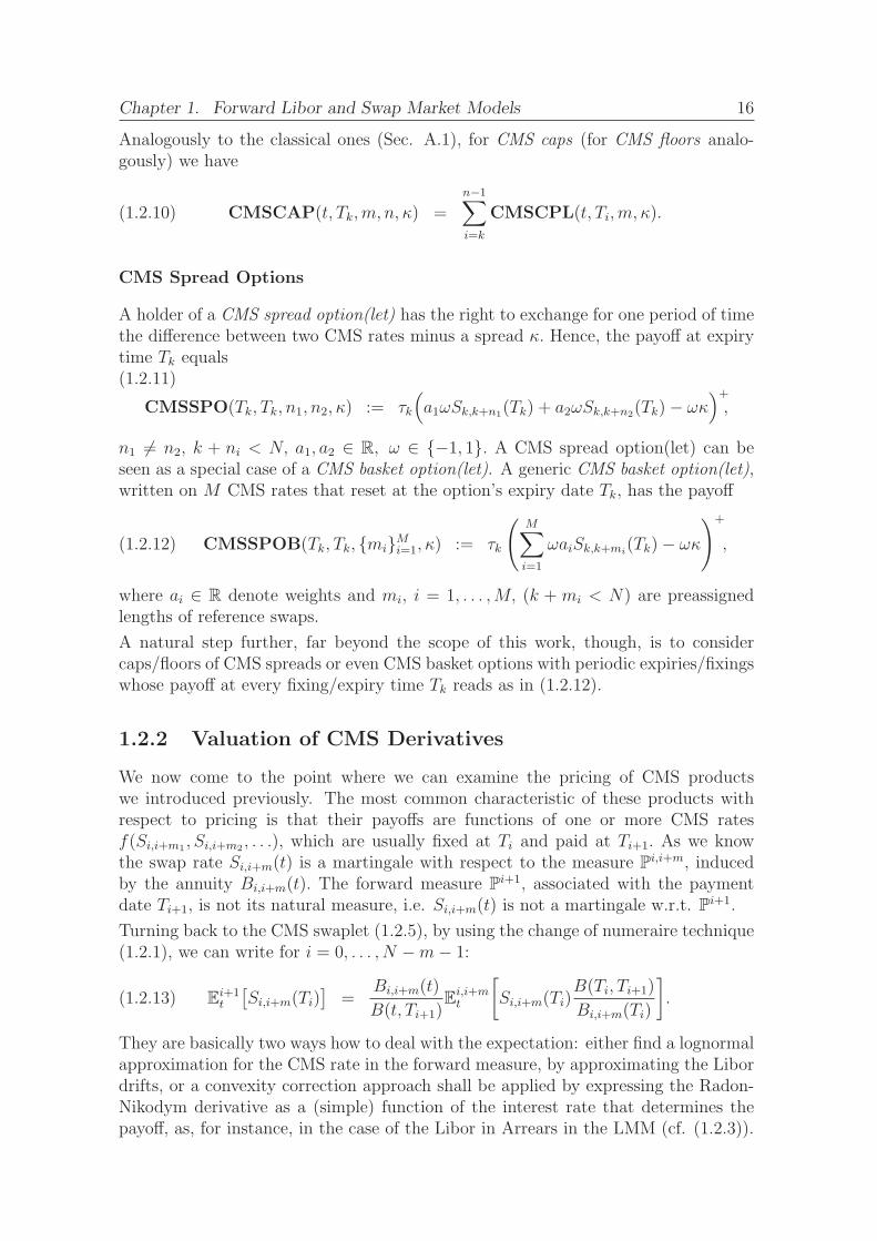
Analogously to the classical ones (Sec. A.1), for CMS caps (for CMS floors analo-gously) we have
CMSCAP(t, Tk,m, n, κ) =n−1∑
i=k
CMSCPL(t, Ti,m, κ).(1.2.10)
CMS Spread Options
A holder of a CMS spread option(let) has the right to exchange for one period of timethe difference between two CMS rates minus a spread κ. Hence, the payoff at expirytime Tk equals(1.2.11)
CMSSPO(Tk, Tk, n1, n2, κ) := τk
(
a1ωSk,k+n1(Tk) + a2ωSk,k+n2
(Tk)− ωκ)+
,
n1 6= n2, k + ni < N, a1, a2 ∈ R, ω ∈ −1, 1. A CMS spread option(let) can beseen as a special case of a CMS basket option(let). A generic CMS basket option(let),written on M CMS rates that reset at the option’s expiry date Tk, has the payoff
(1.2.12) CMSSPOB(Tk, Tk, miMi=1, κ) := τk
(
M∑
i=1
ωaiSk,k+mi(Tk)− ωκ
)+
,
where ai ∈ R denote weights and mi, i = 1, . . . ,M, (k + mi < N) are preassignedlengths of reference swaps.
A natural step further, far beyond the scope of this work, though, is to considercaps/floors of CMS spreads or even CMS basket options with periodic expiries/fixingswhose payoff at every fixing/expiry time Tk reads as in (1.2.12).
1.2.2 Valuation of CMS Derivatives
We now come to the point where we can examine the pricing of CMS productswe introduced previously. The most common characteristic of these products withrespect to pricing is that their payoffs are functions of one or more CMS ratesf(Si,i+m1
, Si,i+m2, . . .), which are usually fixed at Ti and paid at Ti+1. As we know
the swap rate Si,i+m(t) is a martingale with respect to the measure Pi,i+m, induced
by the annuity Bi,i+m(t). The forward measure Pi+1, associated with the payment
date Ti+1, is not its natural measure, i.e. Si,i+m(t) is not a martingale w.r.t. Pi+1.
Turning back to the CMS swaplet (1.2.5), by using the change of numeraire technique(1.2.1), we can write for i = 0, . . . , N −m− 1:
Ei+1t
[
Si,i+m(Ti)]
=Bi,i+m(t)
B(t, Ti+1)E
i,i+mt
[
Si,i+m(Ti)B(Ti, Ti+1)
Bi,i+m(Ti)
]
.(1.2.13)
They are basically two ways how to deal with the expectation: either find a lognormalapproximation for the CMS rate in the forward measure, by approximating the Libordrifts, or a convexity correction approach shall be applied by expressing the Radon-Nikodym derivative as a (simple) function of the interest rate that determines thepayoff, as, for instance, in the case of the Libor in Arrears in the LMM (cf. (1.2.3)).

Chapter 1. Forward Libor and Swap Market Models 17
In this section we want to discuss some of the methods used in the practice to ap-proximate (1.2.13). The first method exploits the idea of making the Radon-Nikodymderivative a function of the payout rate.
Approximating the Radon-Nikodym Derivative and the Convexity Cor-rection
For evaluating (1.2.13) we here recall the convexity approach in Pelsser [2003], basedon the assumption of a lognormal SMM, cf. Hunt-Kennedy [2004]:
B(Ti, Ti+1)
Bi,i+m(Ti)≈ a+ bi+1Si,i+m(Ti),(1.2.14)
where a and bi+1 are constants which are determined as follows. As the Radon-Nikodym derivative is a martingale w.r.t. to the annuity measure, by taking theexpectation we obtain
B(t, Ti+1)
Bi,i+m(t)= E
i,i+mt
[
B(Ti, Ti+1)
Bi,i+m(Ti)
]
= a+ bi+1Si,i+m(t).
Hence,
(1.2.15) bi+1 =1
Si,i+m(t)
(
B(t, Ti+1)
Bi,i+m(t)− a
)
.
On the other hand we have by summing up
1 =i+m−1∑
k=i
τkB(t, Tk+1)
Bi,i+m(t)=
i+m−1∑
k=i
τk (a+ bk+1Si,i+m(t)) .
Replacing bi+1 by (1.2.15),
a =1
∑i+m−1k=i τk
, bi+1 =Bi+1(t)− Bi,i+m(t)
∑i+m−1k=i
τk
Bi(t)−Bi+m(t)(1.2.16)
hold. Finally, we can rewrite (1.2.13) as
(1.2.17) Ei+1t
[
Si,i+m(Ti)]
= Si,i+m(t)
(
1 +bi+1Var
i,i+m[Si,i+m(Ti)]
Si,i+m(t)(a+ bi+1Si,i+m(t))
)
.
The linear approximation in (1.2.14) does seem very crude at first, but can be justifiedby the following argument (cf. Pelsser [2003]). Convexity corrections only becomesizable for large maturities. However, for large maturities the term structure almostmoves in parallel. Hence, a change in the level of the long end of the curve is welldescribed by the swap rate. Furthermore, for parallel moves in the curve, the ratioB(Ti, Ti+1)/Bi,i+m(Ti) is closely approximated by a linear function of the swap rate,which is exactly what the approach does. This leads to a good approximation of theconvexity correction for long maturities.
With these formulas we can easily price linear CMS products like in (1.2.5) – (1.2.6).

Chapter 1. Forward Libor and Swap Market Models 18
In his seminal work Hagan [2003] discusses general approximations of functionalform to the Radon-Nikodym derivative given through (1.2.13). He writes for theCMS caplets:
CMSCPL(t, Ti,m, κ) = B(t, Ti+1)τiEi,i+mt
[
(
Si,i+m(Ti)− κ)+B(Ti, Ti+1)/Bi,i+m(Ti)
B(t, Ti+1)/Bi,i+m(t)
]
= B(t, Ti+1)τiEi,i+mt
[
(
Si,i+m(Ti)− κ)+]
+ B(t, Ti+1)τiEi,i+mt
[
(
Si,i+m(Ti)− κ)+(
B(Ti, Ti+1)/Bi,i+m(Ti)
B(t, Ti+1)/Bi,i+m(t)− 1
)]
.
The first term is exactly the price of a European swaption (cf. (A.3.2)) with notionalB(t, Ti+1)/Bi,i+m(t), regardless of how the swap rate is modeled. The last term is theconvexity correction. Following the argumentation in Hagan [2003], since Si,i+m is a
martingale in the annuity measure andB(Ti,Ti+1)/Bi,i+m(Ti)
B(t,Ti+1)/Bi,i+m(t)− 1 is zero on average, this
term goes to zero linearly with the variance of the swap rate, and is much smallerthan the first term. Giving the ratio a general form
(1.2.18) B(Ti, Ti+1)/Bi,i+m(Ti) = G(Si,i+m(Ti)),
for some function G, we then have
CMSCPL(t, Ti,m, κ) = B(t, Ti+1)τiEi,i+mt
[
(
Si,i+m(Ti)− κ)+]
+ B(t, Ti+1)τiEi,i+mt
[
(
Si,i+m(Ti)− κ)+(
G(Si,i+m(Ti))
G(Si,i+m(t))− 1
)]
.
Using the general property for smooth functions f with f(κ) = 0 (integration byparts):
(1.2.19) f ′(κ)(
S − κ)+
+
∫ ∞
κ
(
S − x)+
f ′′(x) dx =
f(S) for S > κ0 for S < κ,
and choosing
(1.2.20) f(x) =(
x− κ)
(
G(x)
G(Si,i+m(t))− 1
)
,
we obtain by simple transformations
CMSCPL(t, Ti,m, κ) = τiB(t, Ti+1)
Bi,i+m(t)
[
1 + f ′(κ)]
PSWO(t, Ti, Ti+m, κ)
+
∫ ∞
κ
PSWO(t, Ti, Ti+m, x)f′′(x) dx
.(1.2.21)
This formula replicates the value of the CMS caplet in terms of European swaptionsat different strikes It takes into account the presence of a market smile, incorporatingconsistently the information coming from the quoted swaption Black -volatilities. Werefer to Mercurio-Pallavicini [2006] for discussions about the approximation of the
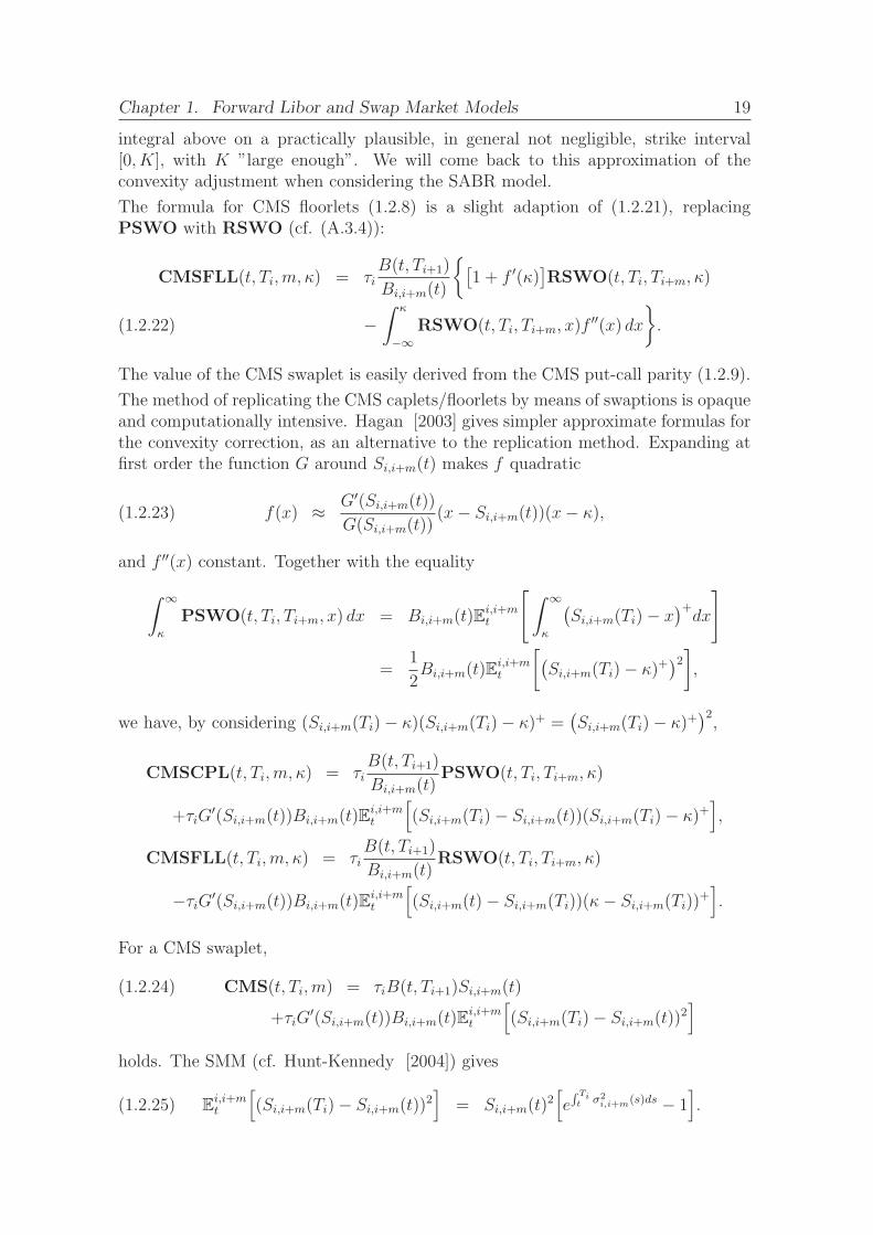
Chapter 1. Forward Libor and Swap Market Models 19
integral above on a practically plausible, in general not negligible, strike interval[0, K], with K ”large enough”. We will come back to this approximation of theconvexity adjustment when considering the SABR model.
The formula for CMS floorlets (1.2.8) is a slight adaption of (1.2.21), replacingPSWO with RSWO (cf. (A.3.4)):
CMSFLL(t, Ti,m, κ) = τiB(t, Ti+1)
Bi,i+m(t)
[
1 + f ′(κ)]
RSWO(t, Ti, Ti+m, κ)
−∫ κ
−∞RSWO(t, Ti, Ti+m, x)f
′′(x) dx
.(1.2.22)
The value of the CMS swaplet is easily derived from the CMS put-call parity (1.2.9).
The method of replicating the CMS caplets/floorlets by means of swaptions is opaqueand computationally intensive. Hagan [2003] gives simpler approximate formulas forthe convexity correction, as an alternative to the replication method. Expanding atfirst order the function G around Si,i+m(t) makes f quadratic
(1.2.23) f(x) ≈ G′(Si,i+m(t))
G(Si,i+m(t))(x− Si,i+m(t))(x− κ),
and f ′′(x) constant. Together with the equality
∫ ∞
κ
PSWO(t, Ti, Ti+m, x) dx = Bi,i+m(t)Ei,i+mt
[
∫ ∞
κ
(
Si,i+m(Ti)− x)+
dx
]
=1
2Bi,i+m(t)E
i,i+mt
[
(
Si,i+m(Ti)− κ)+)2]
,
we have, by considering (Si,i+m(Ti)− κ)(Si,i+m(Ti)− κ)+ =(
Si,i+m(Ti)− κ)+)2,
CMSCPL(t, Ti,m, κ) = τiB(t, Ti+1)
Bi,i+m(t)PSWO(t, Ti, Ti+m, κ)
+τiG′(Si,i+m(t))Bi,i+m(t)E
i,i+mt
[
(Si,i+m(Ti)− Si,i+m(t))(Si,i+m(Ti)− κ)+]
,
CMSFLL(t, Ti,m, κ) = τiB(t, Ti+1)
Bi,i+m(t)RSWO(t, Ti, Ti+m, κ)
−τiG′(Si,i+m(t))Bi,i+m(t)E
i,i+mt
[
(Si,i+m(t)− Si,i+m(Ti))(κ− Si,i+m(Ti))+]
.
For a CMS swaplet,
CMS(t, Ti,m) = τiB(t, Ti+1)Si,i+m(t)(1.2.24)
+τiG′(Si,i+m(t))Bi,i+m(t)E
i,i+mt
[
(Si,i+m(Ti)− Si,i+m(t))2]
holds. The SMM (cf. Hunt-Kennedy [2004]) gives
Ei,i+mt
[
(Si,i+m(Ti)− Si,i+m(t))2]
= Si,i+m(t)2[
e∫ Tit σ2
i,i+m(s)ds − 1]
.(1.2.25)

Chapter 1. Forward Libor and Swap Market Models 20
Given that G(Si,i+m(t)) approximates the ratio B(t, Ti+1)/Bi,i+m(t) (cf. (1.2.18))linear as in (1.2.14)), the equation (1.2.24) perfectly matches with (1.2.17).
Hagan [2003] suggests to use for CMS swaps the volatility of at-the-money swaptions,since the expected value includes high and low strike swaptions equally. For out-of-the-money CMS caplets and floorlets, the strike-specific volatility should be used,while for in-the-money options, the largest contributions come from swap rates nearthe mean value. Accordingly, call-put-parity should be used to evaluate in-the-moneycaplets and floorlets as a CMS swap payment plus an out-of-the-money CMS floorletor caplet.
The function G has been considered a general smooth and slowly varying function,regardless of the model used to obtain it. Hagan [2003] develops simpler approximateformulas for the convexity correction, by specifying G. We shall present here themarket standard method for computing convexity corrections which uses bond mathapproximations and goes as follows. Let the yield curve be flat, fixed at a level y.Then, given an equidistant time grid with step size ∆T and discrete discounting, wecan write
Bi,i+m(t) =i+m∑
k=i+1
τk−1B(t, Tk) =i+m∑
k=i+1
∆TB(t, Ti+1)
(1 + ∆Ty)k−i−1.
The standard formula for the geometric sum gives then
Bi,i+m(t) =B(t, Ti+1)
Si,i+m(t)
[
(1 + ∆TSi,i+m(t))−1
(1 + ∆TSi,i+m(t))m−1
]
,
where the par swap rate y = Si,i+m(t) was taken as discount rate, since it representsthe average rate over the life of the reference swap. Thus,
(1.2.26) Gstd(Si,i+m(t)) =Si,i+m(t)
(1 + ∆TSi,i+m(t))− 1(1+∆TSi,i+m(t))m−1
.
A more accurate lognormal approximation of the swap rates and their correlations inthe forward measure was introduced by Belomestny-Kolodko-Schoenmakers [2010],based on the method of freezing the weights (as in Section 1.1.5) but assuming amore sophisticated approximation.
The approximation (1.2.17) is model independent and quite accurate especially forflat yield curves and highly correlated rates. Such constraints are not necessarilyunrealistic, since adjustments are mostly relevant for long maturities (and tenors),where (forward) rates tend to be constant and to move in parallel fashion.
Assuming lognormal-type dynamics for the swap rates as in SMM we obtain theclassical Black-like adjustment with at-the-money implied volatilities given through(1.2.24)–(1.2.26).
Pricing CMS Spread Options
Once more than one CMS rate is part of a payoff, as in case of CMS spread options,the correlation between the CMS rates in the forward measure starts playing animportant role in pricing these products.

Chapter 1. Forward Libor and Swap Market Models 21
Let us first focus on CMS spread option(let)s with zero strike whose payoff at expirytime Ti equals (cf. (1.2.11))
(1.2.27) CMSSPO(Ti, Ti, n1, n2, 0) := τi
(
Si,i+n1(Ti)− Si,i+n2
(Ti))+
.
The arbitrage-free value of the payoff (1.2.27) at time t is given by
(1.2.28) CMSSPO(t, Ti, n1, n2, 0) := τiB(t, Ti)Eit
[(
Si,i+n1(Ti)− Si,i+n2
(Ti))+]
,
which can be calculated as soon as we know the joint distribution of the pair of swaprates Si,i+n1
and Si,i+n2under the forward measure P
i.
Apart from the fact that the expectation is taken in the non-natural forward mea-sure, this payoff is the one of an exchange option. Therefore, the simplest valuationprocedure is based on assuming that the logarithms of the swap rates are jointly nor-mally distributed as in the Black-Scholes model of two underlying assets. A formaljustification of this approach is given by resorting to the SMM (cf. Def. 1.3) andsuitable approximations. Thus, let assume that both swap rates evolve according to
dSi,i+n1= µi,i+n1
(t)Si,i+n1dt+ σi,i+n1
Si,i+n1dW i
t(1.2.29)
dSi,i+n2= µi,i+n2
(t)Si,i+n2dt+ σi,i+n2
Si,i+n2dW i
t ,(1.2.30)
where W it and W i
t are Brownian motions under Pi, correlated via d(W it , W
it ) = ρ(t)dt,
with ρ(t) assumed to be given (estimated historically or approximated, for instance,as in Belomestny-Kolodko-Schoenmakers [2010]. The drifts µi,i+n1
and µi,i+n2of the
corresponding swap rates with respect to Pi are motivated by (1.1.17) and assumed
to be frozen or deterministic.
The formula for pricing exchange options, developed by Margrabe [1978] using thechange of numeraire technique, can now be applied to obtain:(1.2.31)
Eit
[(
Si,i+n1(Ti)− Si,i+n2
(Ti))+]
= BS
(
Eit[Si,i+n1
(Ti)],Eit[Si,i+n2
(Ti)], σ√
Ti − t, 1)
.
With the swap rate dynamics given in (1.2.29)–(1.2.30) we obtain explicitly:
Eit[Si,i+nk
(Ti)] = Si,i+nk(t)e
∫ Tit µi,i+nk
(s)ds, k = 1, 2,
and
(1.2.32) σ2 =1
Ti − t
∫ Ti
t
(
σ2i,i+n1
(s) + σ2i,i+n2
(s)− 2ρ(s) σi,i+n1(s)σi,i+n2
(s))
ds.
There are several ways how to approximate drifts deterministically under Pi, for
instance:
• they can be inferred from the convexity adjustments, i.e. from the approxima-tions to E
it
[
Si,i+nk(Ti)
]
, k = 1, 2 (discussed in the previous section). We notethat the convexity adjustment technique does not give the correlation betweenthe swap rates w.r.t. Pi;

Chapter 1. Forward Libor and Swap Market Models 22
• the classical method of ”freezing the coefficients” can be applied to (1.1.17),to make the P
i-dynamics of the swap rates lognormal, i.e. Eit
[
Si,i+nk(Ti)
]
=
Si,i+nk(t)eµ
ii,i+nk
(t)(Ti−t), with µii,i+nk
(t) given in (1.1.17);
• complex lognormal approximations, as in Belomestny-Kolodko-Schoenmakers[2010] for instance, can be applied to the swap rates under Pi.
Assuming the dynamics (1.2.29)–(1.2.30) with drifts µii,i+nk
(t), k = 1, 2, and the cor-relation ρ(t) between the two swap rates frozen at evaluation time t, Brigo-Mercurio[2007] gives a formula for the more general case of a time Ti payoff (1.2.11) with astrike κ 6= 0:
(1.2.33) Eit
[(
aωSi,i+n1(Ti) + bωSi,i+n2
(Ti)− ωκ)+]
=
∫ +∞
−∞
1√2π
e−12v2f(v) dv,
where
f(v) = aωSi,i+n1(t) exp
(
µii,i+n1
(t)− 1
2ρ(t)2σ2
i,i+n1(t)
)
τ + ρ(t)σi,i+n1(t)
√τv
× Φ
ωln
aSi,i+n1(t)
h(v)+[
µi,i+n1(t) + (1
2− ρ(t)2)σ2
i,i+n1(t)]
τ + ρ(t)σi,i+n1(t)
√τv
σi,i+n1(t)
√τ√
1− ρ(t)2
− ωh(v)Φ
ωln
aSi,i+n1(t)
h(v)+[
µi,i+n1(t)− 1
2σ2i,i+n1
(t)]
τ + ρ(t)σi,i+n1(t)
√τv
σi,i+n1(t)
√τ√
1− ρ(t)2
,
h(v) = κ− bSi,i+n2(t)e(µi,i+n2
(t)− 12σ2i,i+n2
(t))τ+σi,i+n2(t)
√τv, τ = Ti − t.
A straight-forward calculation shows that for κ = 0 the equation (1.2.31) is recovered.
By no log-normality of the swap rates, an analytical solution for the case κ 6= 0 isonly feasible if the spread is modeled as a normal distributed random variable:
(1.2.34) Si,i+n1(t)− Si,i+n2
(t) = S(t) with dS(t) = σdW (t).
This framework is too simple to consistently price CMS spread options since implicitlya perfect correlation is assumed. And it is also not taking into account the smileand the skew effects. The market quotes spread options by their implied normalvolatilities, similar to swaptions which are quoted by their implied Black volatility.
1.3 Parameterization and Calibration
The general form of the forward Libor model (cf. Def. 1.1) is merely a frameworkwhich becomes a model once the forward volatility structure γi(t), i ∈ 0, . . . , N−1,is specified, which determines both the level of the forward rates and the correlationbetween the forward rates via
ρi,j(t) =γi(t) · γj(t)
‖γi(t)‖‖γj(t)‖, 0 ≤ t ≤ minTi, Tj.
Chapter 1. Forward Libor and Swap Market Models 23
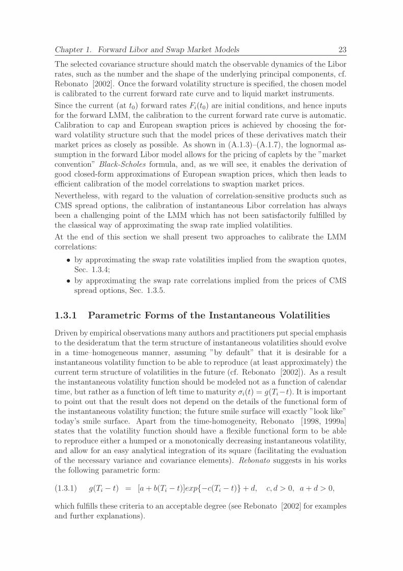
The selected covariance structure should match the observable dynamics of the Liborrates, such as the number and the shape of the underlying principal components, cf.Rebonato [2002]. Once the forward volatility structure is specified, the chosen modelis calibrated to the current forward rate curve and to liquid market instruments.
Since the current (at t0) forward rates Fi(t0) are initial conditions, and hence inputsfor the forward LMM, the calibration to the current forward rate curve is automatic.Calibration to cap and European swaption prices is achieved by choosing the for-ward volatility structure such that the model prices of these derivatives match theirmarket prices as closely as possible. As shown in (A.1.3)–(A.1.7), the lognormal as-sumption in the forward Libor model allows for the pricing of caplets by the ”marketconvention” Black-Scholes formula, and, as we will see, it enables the derivation ofgood closed-form approximations of European swaption prices, which then leads toefficient calibration of the model correlations to swaption market prices.
Nevertheless, with regard to the valuation of correlation-sensitive products such asCMS spread options, the calibration of instantaneous Libor correlation has alwaysbeen a challenging point of the LMM which has not been satisfactorily fulfilled bythe classical way of approximating the swap rate implied volatilities.
At the end of this section we shall present two approaches to calibrate the LMMcorrelations:
• by approximating the swap rate volatilities implied from the swaption quotes,Sec. 1.3.4;
• by approximating the swap rate correlations implied from the prices of CMSspread options, Sec. 1.3.5.
1.3.1 Parametric Forms of the Instantaneous Volatilities
Driven by empirical observations many authors and practitioners put special emphasisto the desideratum that the term structure of instantaneous volatilities should evolvein a time–homogeneous manner, assuming ”by default” that it is desirable for ainstantaneous volatility function to be able to reproduce (at least approximately) thecurrent term structure of volatilities in the future (cf. Rebonato [2002]). As a resultthe instantaneous volatility function should be modeled not as a function of calendartime, but rather as a function of left time to maturity σi(t) = g(Ti−t). It is importantto point out that the result does not depend on the details of the functional form ofthe instantaneous volatility function; the future smile surface will exactly ”look like”today’s smile surface. Apart from the time-homogeneity, Rebonato [1998, 1999a]states that the volatility function should have a flexible functional form to be ableto reproduce either a humped or a monotonically decreasing instantaneous volatility,and allow for an easy analytical integration of its square (facilitating the evaluationof the necessary variance and covariance elements). Rebonato suggests in his worksthe following parametric form:
(1.3.1) g(Ti − t) = [a+ b(Ti − t)]exp−c(Ti − t)+ d, c, d > 0, a+ d > 0,
which fulfills these criteria to an acceptable degree (see Rebonato [2002] for examplesand further explanations).

Chapter 1. Forward Libor and Swap Market Models 24
(1.3.1) can be extended to a richer parametric form; the extended linear-exponentialvolatility model (cf. Rebonato [2002], Brigo-Capitani-Mercurio [2003]):
(1.3.2) gext(Ti − t) = kig(Ti − t), k(Ti) > 0.
Rebonato [2002] models the vector k ∈ RN as ki = 1 + ǫ(Ti), being ideally close to
one and flexible enough to allow for a better fit of volatility function to the marketimplied volatilities of different maturities.
Assuming no smile and skews in the caplet markets, any choice of the parametersa, b, c, d will only approximately satisfy the ATM caplet condition,
(1.3.3) (σBlack
i )2 (Ti − t) =
∫ Ti
t
g(u)2 du,
across all forward rates8. The parameters ki then allow for the Libor rate specificadjustment to exactly fit the market implied volatility:
(1.3.4) k2i =
(σBlack
i )2 (Ti − t)∫ Ti
tg(u)2 du
.
The caplet condition (1.3.3) is then fulfilled by construction everywhere along thecurve.
A good and extensive overview of the volatility parameterizations used in practicecan be found in Brigo-Mercurio [2007].
1.3.2 Calibration to the Cap/Floor Market
The market convention to quote caps and floors is to use the (implied) Black- volatilitywhich plugged into the Black formula gives the market price of the cap/floor. In asmile-less world, we know from the Black-Scholes theory that for the instantaneousvolatility function σi(t) of a forward rate Fi(t) in the lognormal LMM the impliedBlack volatility σBlack
i is given by (cf. (A.1.4)),
(1.3.5) (σBlack
i )2 (Ti − t) =
∫ Ti
t
σi(u)2 du.
Ideally, in case of given market prices of ATM caplets, their implied Black volatilityconstitutes the right value to fit with the model volatility parameters.
The market prices are unfortunately a bit more involved. The market quotes flatvolatilities for caps of different maturities, T and strikes, K. Thus, an implied volatil-ity surface σBlack
cap(T,K) is quoted at any point in time. So what are the implied
volatilities of the caplets that make up the caps with different strikes and maturi-ties that are consistent with the quoted cap volatility surface? Alexander [2003]gives a brief and good overview about the particularities in stripping the informationout of cap market prices. For instance, each fixed strike caplet in a cap with the
8Depending on the calibration target one can choose the model volatility parameters to meetcondition (1.3.3) even not (only) for ATM Black volatilities.

Chapter 1. Forward Libor and Swap Market Models 25
ATM strike K has a different moneyness. Each Ti maturing caplet is assumed to beATM if Fi(Ti) = K, but since each caplet has a different underlying forward rate, itwill have a different ATM strike. So the different caplets in an ATM cap are onlyapproximately ATM. One of the popular iterative methods, used to back out thesecaplet volatilities from the cap market implied volatility surface, is the vega-weightedinterpolation technique, for which we refer to Alexander [2003].
Several stripping algorithms9 to extracting caplet volatilities out of quoted cap volatil-ities are presented in detail in the technical work by Hagan-Konikov [2004].
Finally, in a smile-less world, the calibration to caplets’ and floorlets’ implied volatil-ities (once extracted from the market quotes of caps and floors) for the LMM model isstraight-forward via (1.3.5), and the correlations between forward Libor rates have noimpact on the cap/floor prices. The application of the calibration requirement (1.3.5)to the volatility parameterizations given above is straight-forward as well. Therefore,in the sequel we will focus on the parameterization given in (1.3.2)–(1.3.4). The firststep in the calibration procedure is to find the solution parameters a, b, c, d for theminimizing problem(1.3.6)
mina,b,c,d
N−1∑
i=0
[
σBlack
i
√
(Ti − t)−√
∫ Ti
t
[
[a+ b(Ti − t)]exp−c(Ti − t)+ d]2
du
]2
.
Additionally, the free Libor rate specific parameters ki in (1.3.4) can be used toexactly fit the respective (ATM) Black caplet volatilities.
1.3.3 The Structure of Instantaneous Correlations
As discussed in Sec. 1.1.3, both, the instantaneous volatility formulation as well asthe chosen instantaneous correlation, can contribute to terminal correlations. Thequalities and properties an instantaneous correlation matrix ρ associated with a LMMshould have are (cf. Brigo-Mercurio [2007]):
• Symmetry and ones on the diagonal:
ρi,j = ρj,i, ρi,i = 1, for all i, j ∈ 0, . . . , N − 110;
• ρi,j ≥ 0 for all i, j, and the map i 7→ ρi,j has to be decreasing for i ≥ j,thus, moving away from the diagonal along a column or row the entries becomemonotonically decreasing as joint movements of far away rates are less correlatedthan movements of the rates with close maturity;
• When moving along the yield curve, the larger the tenor, the more correlatedthe adjacent forward rates are. Hence, the sub-diagonals, i 7→ ρi+p,i, will beincreasing for a fixed p.
9The idea behind the boot-stripping algorithms is that if we know, for instance, the 1 and 2 yearflat volatilities we know the 1 year and 2 year cap prices. Their price difference is by no arbitragearguments the second caplet in 2 year cap contract. It is thus required to solve a volatility thatimplies this caplet price. The same procedure is continued iteratively further.
10For ease of notation we will be numbering the elements of the correlation matrix by beginningwith zero, ρ = ρi,jN−1
i,j=0, coinciding with the numbering of the forward rates and their expiries.

Chapter 1. Forward Libor and Swap Market Models 26
A variety of parameterization functions have been introduced over the past years thatallow for expressing a given correlation matrix of forward rates in a functional form.There are several advantages to this: of course, it is computationally convenientto work with an analytical formula. But also noise, such as bid-ask spreads, andilliquidity are removed by focusing on general properties of correlation. Furthermore,the rank and the positive semi-definiteness of the correlation matrix can be controlledthrough the functional form.
The parameterizations we shall present here are full-rank parameterizations. Wewill also discuss how to reduce their rank depending on the number of underlyingBrownian motions of the model. One property that is implicitly present in all pa-rameterizations is the desirable time-homogeneity of the correlations.
Full-rank correlation parameterization
In general, the full instantaneous correlation matrix is characterized by N(N − 1)/2entries, given the symmetry and the ones on the diagonal. This number of entriesmay be too high for practical purposes, thus, a parsimonious parametric form withreduced number of parameters has to be found. In the literature a vast number ofcorrelation parameterizations is presented; to be mentioned here are the works ofSchoenmakers-Coffey [2003], Wu-Zhang [2003], Morini-Webber [2006], and latelythe papers of Borger-van Heys [2010] and Lutz [2010].
We will focus in the sequel on some of the parameterizations which will be used inour model calibration later on.
Three-parameters full-rank exponential parameterization. For 0 ≤ t ≤minTi, Tj Rebonato [2004] proposed a parameterization of the form
(1.3.7) ρi,j(ρ∞, α, β; t) = ρ∞ + (1− ρ∞) exp[
− |Ti − Tj|(β − αmaxi, j)]
,
which fulfils the desirable properties given above. Thus, it may produce for a giventenor structure realistic market correlations for properly chosen ρ∞ ∈ (−1, 1), β > 0and (small) 0 ≤ α ≤ β/(N − 1) (cf. Rebonato [1999a]). A slight modification of(1.3.7), also given in Rebonato [2004], reads:
(1.3.8) ρi,j(ρ∞, α, β; t) = ρ∞ + (1− ρ∞) exp[
− β|Ti − Tj| exp
−αmaxi, j
]
,
with ρ∞ ∈ (−1, 1), β > 0 and α ∈ R.
A special case of (1.3.7) is the Rebonato’s two-parameters full-rank exponential pa-rameterization:
(1.3.9) ρi,j(ρ∞, β; t) = ρ∞ + (1− ρ∞) exp[
− β|Ti − Tj|]
, β > 0, ρ∞ ∈ (−1, 1).
However, it should be noted that for a particular choice of parameters it is not directlyguaranteed that (1.3.7) or (1.3.8) defines valid correlation structure indeed (it mightviolate the positive semi-definiteness of the correlation matrix). The special case withρ∞ = 1 (cf. Rebonato [2002]),
(1.3.10) ρi,j(β; t) = exp[
− β|Ti − Tj|]
, t ∈ [0, Ti ∧ Tj],

Chapter 1. Forward Libor and Swap Market Models 27
assures a symmetric correlation matrix with positive eigenvalues. This parameteri-zation is analytically very attractive and fulfills the basic modeling requirements.
Apart from their parameter poorness which might turn out to be a handicap whenfitting to market quotes, these parameterizations do not distinguish on the distancebetween two different forward rates such that different pairs of forward rates with thesame distance to each other are correlated to the same degree. Since an unconstrainedoptimization is preferable to a constrained one, Schoenmakers-Coffey [2003] param-eterizations might be preferred from this point of view. Nonetheless, the Rebonato’sparameterizations are widely used in practice because of their analytical tractabilityand the easy calibration.
Doust ’s multiplicative correlations (cf. Doust [2007], Rebonato-McKay-White[2009]). To overcome the above-mentioned problem that the decorrelation (broughtinto the model by the constant exponential decay factor β) only depends on thedistance between two rates, the challenge will be to introduce a dependence of thedecorrelation factor on the expiries of the forward rates, β = βi,j , in such a way thatthe resulting correlation matrix does not loose any of the desired properties of beinga valid correlation matrix.
Similar in spirit to the construction in Schoenmakers-Coffey [2003], Doust proposesthe following parametric structure (cf. Doust [2007]):For ai ∈ [−1, 1],11 i = 1, . . . , N−112 the elements of the correlation matrix are definedrecursively:
- First define the trivial diagonal elements, ρi,i = 1, i = 0, . . . , N − 1;- Then define the elements of the first row by respecting the symmetry as
ρ0,j =
j∏
k=1
ak = ρj,0, j = 1, . . . , N − 1;
- By inspection, assuming that i > j, fill the lower triangle part by
ρi,j =ρ0,iρj,0
=i∏
k=j+1
ak.
The upper triangle part is then defined by the symmetry relationship:
ρ(a1, ..., aN−1; t) =
1 a1 a1a2 a1a2a3 . . . a1 · · · aN−1
a1 1 a2 a2a3 . . . a2 · · · aN−1
a1a2 a2 1 a3 . . . a3 · · · aN−1...
. . . . . . . . ....
a1 · · · aN−2 . . . aN−2 1 aN−1
a1 · · · aN−1 . . . aN−1 1
.
Given the N − 1 quantities ai, Doust [2007] proves that the resulting matrix isalways a real symmetric positive definite matrix which admits a simple Cholesky
11In the most cases ai will be positive, 0 < ai ≤ 1, as, empirically, the forward rate – forward ratecorrelations are proven to be positive.
12Recall that a correlation matrix has got N(N−1)/2 elements to be specified; here we are dealingwith N − 1 unknown parameters.

Chapter 1. Forward Libor and Swap Market Models 28
decomposition. Given an equidistant time grid ∆T = Ti+1 − Ti, i = 0, . . . , N − 1,(i.e. constant spacing between the forward rates in the considered model) Rebonato-McKay-White [2009] suggests the following choice of the parameters ai:
(1.3.11) ak = exp−βk∆T, k = 1, . . . , N − 1.
Then we have for i > j
(1.3.12) ρi,j(β1, ..., βN−1; t) = exp
−i∑
k=j+1
βk∆T
, 0 ≤ t ≤ minTi, Tj.
The dependence of βk on k allows us to specify the degree of decorrelation be-tween rates with same distance but different expiries. A decreasing property of βk :βk > βk+1, is empirically evident. Obviously, for a constant βk ≡ β, the simple pa-rameterization in (1.3.10) will be recovered. The flexibility can be even increased byintroducing functional forms to describe the dependence of βk > 0 on k. Polynomialforms of degree M ≤ N − 1, PM , like
(1.3.13) βk = PM(k) =M∑
l=0
gl/kl,
with positive parameters gl, easily guarantee the desired properties of the matrix.The correlation parameterization then takes for i > j the shape
(1.3.14) ρi,j(g0, ..., gM ; t) = exp
−∆T
i∑
k=j+1
M∑
l=0
gl/kl
, t ∈ [0, Ti ∧ Tj].
Finally, Rebonato-McKay-White [2009] go one step further imposing an additionallong-term decorrelation among the forward rates, preventing that the decorrelationgoes asymptotically to zero with increasing distance between the rates, but rather tosome finite economically plausible level ρ∞ > 0:
(1.3.15) ρi,j(ρ∞, g0, ..., gM ; t) = ρ∞ + (1− ρ∞)ρi,j(g0, ..., gM ; t), t ∈ [0, Ti ∧ Tj ].
Most of the introduced parameterizations are discussed with great detail in Rebonato[2004], while Schoenmakers [2002] is a good reference for the particularities of theirnumerical implementation and performance.
Rank-Reduced Correlations
From the standard matrix calculus it is well known that any positive semi-definitesymmetric matrix ρ ∈ R
N×N can be diagonalized by means of a real and orthogonalmatrix P ∈ R
N×N :
(1.3.16) ρ = PDP⊥, with PP⊥ = P⊥P = I,
where D ∈ RN×N is the diagonal matrix containing the positive eigenvalues of the
original matrix ρ, whereas the columns of P are the eigenvectors of ρ.Setting B := P
√D we obtain
(1.3.17) ρ = BB⊥ and B⊥B = D.

Chapter 1. Forward Libor and Swap Market Models 29
Rebonato [1999a] mimics the decomposition (1.3.17) by means of a suitable matrixB ∈ R
N×d of rank d < N such that BB⊥ is a d-rank correlation matrix.
In Rebonato [1999a] it is stated and proved that for any real matrix B ∈ RN×d
with rank d ≤ N, the matrix product BB⊥ is real and symmetric, and it can bediagonalized into
BB⊥ = PDP⊥,
where P ∈ RN×d is an orthogonal matrix containing the orthogonal eigenvectors of
BB⊥ and D ∈ Rd×d a diagonal matrix storing the squares of the eigenvalues of BB⊥.
This result is obviously very useful in the parametrization of a d-factor Libor model.As we will see it shall allow us to reduce to a very large extent the difficulties in thesimultaneous calibration to volatilities and to the correlation matrix.
Moreover, it is this result which completes the model picture started in (1.1.5)–(1.1.7), where already a low-factor Brownian shock was anticipated. It can be easilyseen that the introduced matrix B coincides with the matrix containing the loadingvectors bi as row vectors:
B = b⊥(t) =[
b0(t), . . .bN−1(t)]⊥
at any time t.
Here we shall present the two mostly used rank reduction techniques.
The Hypersphere Decomposition. Rebonato-Jaeckel [1999] suggests the fol-lowing form of the i-th column vector of the matrix b in (1.1.7):
bi,k(t) =
cos (θi,k(t))∏k−1
j=1 sin (θi,j(t)) if k = 1, . . . , d− 1∏k−1
j=1 sin (θi,j(t)) if k = d,(1.3.18)
where the angles θi,j(t) constitute the parameters to be altered within the fittingoptimization algorithm. We denote the resulting low-rank correlation matrix by ρθ.
The Spectral Decomposition. Following Rebonato-Jaeckel [1999] an alternativeand effective way of rank-reduction is the so-called spectral decomposition. Given atarget number of driving factors d and assuming (1.3.16) we can arrange the eigen-values in D in descending order and rearrange in P the corresponding eigenvectorssuch that their numbering in columns corresponds to the order of eigenvalues in thenew D:
ρ(t) = P(t)D(t)P⊥(t).
Then the smallest N − d eigenvalues will be set to zero and the corresponding eigen-vectors will be taken off the matrix P(t), resulting in the approximative correlationmatrix
ρ(d)(t) = P(d)(t)D
(d)(t)(P
(d))⊥(t).
In general the resulting matrix ρ(d)(t), although positive semidefinite, does not nec-essary feature ones on its diagonal. The solution is to interpret ρ(d)(t) as a covariancematrix and to derive the correlation matrix associated with it by normalizing it:
ρ(d)i,j (t) =
ρ(d)i,j (t)
√
ρ(d)i,i (t)ρ
(d)j,j (t)
.

Chapter 1. Forward Libor and Swap Market Models 30
By following this procedure we obtain an acceptable correlation matrix ρ(d)(t) whichis a d-rank approximation and intuitively similar to the target one.
This methodology can be found in the literature as the principal component analysis(PCA).
Approach to Optimizing on a Low Rank Parametric Form Once the targetfull-rank correlation matrix ρmod is given as input, we can minimize over the angleparameters θi,j(t) (cf. (1.3.18)) the norm of the difference between the target matrixρmod and the low-rank matrix ρθ:
minθi,j(t)
N∑
i,j=1
(
|ρmod
i,j (t)− ρθ
i,j(t)|2)
.
Rebonato-Jaeckel [1999] proved empirically that the differences between the reduc-tion over the angles and the spectral decomposition is typically very small.
In general, when we calibrate the LMM to swaptions using the instantaneous corre-lations ρ as fitting parameters, as we will see below, we are free to select a-priori aparametric form for the correlation matrix. Once the model matrix of instantaneouscorrelations ρmod is defined we can use one of the introduced rank reduction algorithmsto reduce the degrees of freedom for the random shocks we will use to simulate theforward term structure for future times and price interest rate derivatives.
1.3.4 Calibration of LMM Correlations to Swaptions Volatil-ities
The market is quoting the swaptions in terms of their Black implied volatilities. Forinstance, a Tm × (Tn − Tm) ATM payer swaption with expiry at Tm on the swap rateSm,n(t) is conventionally quoted as σBlack
m,n .
Calibrating the LMM consists of finding the instantaneous volatility σi(t)i andcorrelation parameters ρ(t) in the LMM dynamics that reflect the swaptions pricesobserved in the market. Combining the equations (A.3.3) and (1.1.23) we obtain
(1.3.19)(
σBlack
m,n
)2(Tm − t) =
n−1∑
i,j=m
∫ Tm
t
vm,ni (s)vm,n
j (s)Fi(s)Fj(s)
S2m,n(s)
γi(s) · γj(s) ds.
A sufficiently good and market proven approximation of (1.3.19) is the following:
(1.3.20)(
σBlack
m,n
)2(Tm − t) =
n−1∑
i,j=m
vm,ni (t)vm,n
j (t)Fi(t)Fj(t)
S2m,n(t)
∫ Tm
t
γi(s) · γj(s) ds,
which we shall consider as the standard approach.
1.3.5 Calibration to Correlations Implied From CMS SpreadOptions
Among practitioners and academics alike, there is consensus on the fact that even thelow-parametric LMM correlation parameterizations can hardly be calibrated reliably

Chapter 1. Forward Libor and Swap Market Models 31
to market data due to the fact that swaptions carry only little information about cor-relations (Alexander [2003], Brigo-Mercurio [2007], Rebonato [2002], Schoenmakers[2002, 2005], Schoenmakers-Coffey [2003]).
The market of structured interest rate products, in particular pay-off structures in-cluding derivatives of constant maturity swaps, has undergone an enormous growthduring the past few years. As already discussed in Sec. 1.2.2, such structures equippedwith call rights such as CMS spread options, require a realistic modeling of not onlythe development of swap rates, but also their correlation. Such correlation infor-mation is meanwhile available, because a separate market has developed for spreadoptions used for hedging purposes almost like plain vanilla instruments.
Assuming jointly lognormal swap rates we can work out an implied correlation of theinvolved swap rates in a CMS spread option. This correlation can then be taken astarget to be reproduced by a pricing model and, therefore, has to be included in amodel calibration procedure of LMM.
Motivated by the general formula for the valuation of the CMS spread optionlet givenin (1.2.33), assuming log-normality of the swap rates under Pi, with Ti the expiry timeof the optionlet, Borger-van Heys [2010] propose a calibration of the parameterizedinstantaneous forward rate correlations to prices of CMS spread options. Regarding(1.2.33), the value of a CMS spread optionlet can be written as(1.3.21)
Eit
[(
ωSi,i+n1(Ti)−ωSi,i+n2
(Ti)−κ)+]
= F(
Si,i+nk(t), µi
i,i+nk(t), σi,i+nk
(t), ρ(t), Ti, κ)
,
where k = 1, 2. Applying the typical freezing for the drifts µii,i+nk
(t) of the swap ratesunder P
i, and deriving the swap rate volatilities σi,i+nk(t) from the given market
quotes of the swaption ATM-implied volatilities (as in (A.3.3)), (1.3.21) can now beconsidered as a target function for the swap rate correlation ρ(t), and also for theforward rate correlations through
ρ(t) =1
(Ti − t)σi,i+n1(t)σi,i+n2
(t)
i+n1−1∑
k=i
i+n2−1∑
l=i
vi,i+n1
k (t)vi,i+n2
l (t)Fk(t)Fl(t)
Si,i+n1(t)Si,i+n2
(t)
×∫ Ti
t
σl(s)σk(s)ρl,k(s) ds.(1.3.22)
Here we used a standard approximation, cf. Belomestny-Kolodko-Schoenmakers[2010], for the swap rate correlation. This approach to the calibration of the Li-bor rate correlations was treated as a improvement of the typical market practice ofcalibration to swaption volatilities, showing satisfactory results for certain parame-terization of the instantaneous correlations, such as in Schoenmakers-Coffey [2003].We refer for the details to Borger-van Heys [2010].
The latter underpins our motivation for calibrating the forward rate correlation ofthe more involved SABR–LMM model we shall introduce in Chap. 3.2.

Chapter 2
The SABR Model ofForward Rates
2.1 General Model Dynamics
As already mentioned in Chap. 1.1, one problem encountered when modeling deriva-tives like caplets in the LMM and therefore using the Black formula is, that the marketprices for caplets over different strikes cannot be obtained with a constant volatilityparameter as the model demands1. The presence of these volatility skews and smilesin the market is however evidence that the underlying is driven by some process otherthan a lognormal one. With this in mind Dupire [1994] proposed the local volatilitymodel, which has the advantage that the model perfectly replicates the current mar-ket situation. But the approach behaves poorly in forecasting future dynamics andoption pricing is not possible in closed form. Thus, it became of practical interestto develop stochastic versions of the volatility structures of forward Libor modelscapable of matching the observed volatility in the markets of caps and swaptions, byconsidering a more general volatility process of the form γ(t, T, S;F (t, T, T ∗))2.
It was the seminal work of Hagan et al. [2002] who launched the so called SABRmodel, where the forward rate process is modeled under its forward measure using acorrelated lognormal stochastic volatility process. Hagan et al. [2002] explain clearlywhy ”just fitting the today’s market prices” is not good enough. Taking into accountthe quality of prediction of the future dynamics of the volatility smile, meeting theobservations from the market reality, is as crucial as the best achievable fitting to thetoday’s market prices.
Hagan and his colleagues were not the first to equip BGM-type models with stochasticvolatility, see for instance the Cox-Ingersoll-Ross (CIR)-type models of Andersen-Andreasen [2002], Andersen-Brotherton-Ratcliffe [2005], Piterbarg [2003, 2005a,b]or models of jump-diffusion. All these models lack the ability to fit accurately the
1It should be mentioned that the generic BGM framework does not necessarily require the forwardvolatility functions of forward rates to be deterministic functions; they may be adapted processesor some deterministic or random functions of the underlying forward Libor rates.
2Nevertheless, the class of models of practical interest are mainly characterized by a separa-ble volatility structure, cf. Andersen-Andreasen [2002], Andersen-Brotherton-Ratcliffe [2005],Andersen-Piterbarg [2007], Piterbarg [2003, 2005a,b], Wu-Zhang [2006], etc.
32

Chapter 2. The SABR Model of Forward Rates 33
appropriate market smile surface in a simple fast and robust manner. It is the abilityto do so which constitutes one major advantage of the SABR model, as there existsan approximation formula to implied Black volatility using the SABR parameters,introduced by Hagan et al. [2002]. Hence, option prices, such as of caps and floors, canbe calculated using the well known Black pricing framework but taking into accountthe volatility surface using a strike dependent volatility function. Nowadays theSABR model has become a reference stochastic volatility framework for modelingsmiles in the financial industry, because of the described properties and its easyapplication.
The SABR model attempts to capture the dynamics of a single forward rate. De-pending on the context, this forward rate could be a Libor forward rate, a forwardswap rate, the forward yield on a bond, etc. However, we shall focus in the followingon the SABR model of forward Libor rates.
Definition 2.1 (multifactor SABR Model). Assume that the number of model fac-tors, that is the number of independent driving Brownian motions, is d+ d under theforward measure P
i+1, for the index i ∈ 0, . . . , N − 1.Building on the preliminary framework presented in Chap. 1 for the classical LMM,the (d × d)–factor SABR model (SABR) assumes the following dynamics for theforward rate Fi under its payoff measure P
i+1:
(2.1.1) dFi(t) = Fβi(t)i (t)σi(t) bi(t)·dWi+1
t , 0 ≤ t ≤ Ti,
where 0 ≤ βi(t) ≤ 1 and σi(t) is a stochastic variable following a diffusion process oftype3:
(2.1.2) dσi(t) = σi(t)νi(t) bi(t)·dWi+1
t , 0 ≤ t ≤ Ti,
where Wi+1t is a d-dimensional and W
i+1
t a d-dimensional independent standardBrownian motion under P i+1, and νi(t) the exogenously given deterministic volatilityof volatility function4.
The loading vectors5 bi(t) ∈ Rd and bi(t) ∈ R
d satisfy ‖bi(t)‖d = ‖bi(t)‖d = 1 andfor 0 ≤ t ≤ minTi, Tj:
bi(t)Tbj(t) = ρi,j(t),(2.1.3)
mind,d∑
k=1
bik(t)bjk(t) = φi,j(t), φi,i(t) = ξi(t),(2.1.4)
bi(t)T bj(t) = θi,j(t), j = 0, . . . , N − 1,(2.1.5)
3Note that there is no mean reversion for the volatility process. Since we are looking at oneforward rate at a time, this is not necessarily a problem as long as the correct terminal distributionof the forward rate is obtained.
4While Pi+1, induced by B(t, Ti+1), is a natural martingale measure for the forward rate Fi(t),due to its definition in (1.1.1), the fact that the volatility process in (2.1.2) is defined to be driftlessunder Pi+1 is rather ”artificial” and can be seen as a model assumption.
5For ease of notation we will be numbering the elements of all correlation matrices by beginningwith zero such that they coincide with the numbering of the forward rates.

Chapter 2. The SABR Model of Forward Rates 34
where the matrices ρ(t),φ(t),θ(t) ∈ RN ×R
N are exogenously defined, with the par-ticularity that φ(t) has got ξi(t) = (ξ(t))i, the correlation between the forward rateand its own volatility process, on the diagonals (instead of ones)6.
Imposing the initial conditions for the forward rate process Fi(0) and its initial volatil-ity σi(0) = σSABR
i , the model becomes fully specified.
Investigating the qualitative behavior of the (Black) volatility implied from the SABRmodel, Rebonato-McKay-White [2009] spotted the following properties for the SABRparameters:
• a change (upwards) of the SABR initial volatility σSABR
i causes an almost shift(upwards) of the implied volatility smile across strikes, and a modest steepeningof the smile (low strikes increase more than high strikes);
• when the exponent βi goes from 1 to 0, it causes a progressive steepening ofthe smile and introduces modest curvature to it, while, on the other hand, anincreasing β lowers the level of the smile;
• a similar effect as for decreasing βi can be spotted when the correlation parame-ter ξi moves from 0 to −0.5; the smile becomes negatively slopped, accompaniedwith small decrease in curvature. There seems to be a pronounced redundancyin the resulting effects in choosing the parameters βi and ξi; the prevalent mar-ket practice is to fix the exponent βi (usually at 0.5) and optimize the fittingover the other parameters;
• finally, νi caters for the curvature of the smile (increasing νi increases the cur-vature), with certain secondary effect on the steepness of the smile.
However, only the interaction of all these parameters together makes the model suc-cessfully capable to capture the different market volatility smile surfaces. For deeperdiscussions about the solvability of the SABR system for different CEV exponents βand the property of the dynamics whether zero or negative rates are attainable werefer to the extensive analysis done in Rebonato-McKay-White [2009].
Rebonato-McKay-White [2009] provides a good empirical overview of the strengthsof the SABR model with respect to recovering the dynamics of the smile evolutionwhen the underlying changes, emphasizing, in particular, the aspects of hedging ofthe interest rate risk.
2.1.1 The Time-Homogeneous Model
Definition 2.2 The multifactor time–homogeneous SABR model is a special case ofthe model described in Def. 2.1. The alteration consists of the constant parametersover time:
βi(t) ≡ βi ∈ [0, 1],
νi(t) ≡ νi ∈ R,
6Here we assume that the matrices ρ(t) and θ(t) are valid correlation matrices (cf. Sec. 1.3.3).The slightly modified matrix φ(t) = (φi,j(t))i6=j and (φ(t))i,i = 1 is assumed to be a valid correlationmatrix as well.

Chapter 2. The SABR Model of Forward Rates 35
and time–homogeneous correlation matrices for 0 ≤ t ≤ minTi, Tjbi(t)
Tbj(t) = ρi,j(Tj − Ti),(2.1.6)
mind,d∑
k=1
bik(t)bjk(t) = φi,j(Tj − Ti), φi,i(0) = ξi,(2.1.7)
bi(t)T bj(t) = θi,j(Tj − Ti).(2.1.8)
Imposing the initial conditions for the forward rate process Fi(0) and its volatilityprocess σi(0) = σSABR
i , the model becomes fully specified.
2.1.2 Joint Dynamics of the SABR Forward Rates and Their
Volatilities
Applying the same change of measure technique as in Sec. 1.1.1, in order to derive thearbitrage–free dynamics of the system of the SABR forward rates and their volatilitiesin a single measure, say P
k+1, able to be implemented in practice, we obtain for j < k(j > k analogously):
dB(t, Tj+1)
B(t, Tk+1)=
B(t, Tj+1)
B(t, Tk+1)
k∑
i=j+1
τi1 + τiFi(t)
dFi(t) +O(dt2),
Consequently the following general drift formula for the forward rates in the SABRmodel at time 0 ≤ t ≤ Tj can be derived (cf. Sec. 1.1.1):(2.1.9)
dFj(t) = Fβj
j (t)γj(t)·dWk+1t + σj(t)F
βj
j dt
−k∑
i=j+1
τiFβii (t) σi(t)ρi,j1+τiFi(t)
, j < k
0 , j = kj∑
i=k+1
τiFβii (t) σi(t)ρi,j1+τiFi(t)
, j > k,
where γj = σj(t)bj(t). Analogously, the arbitrage free dynamics with respect to Pk+1
of the volatility parameters in the SABR model is given by (νj(t) = νj bj(t)):(2.1.10)
dσj(t) = σj(t)νj(t)·dWk+1
t + νjσj(t) dt
−k∑
i=j+1
τiFβii (t) σi(t)φi,j
1+τiFi(t), j < k
0 , j = kj∑
i=k+1
τiFβii (t) σi(t)φi,j
1+τiFi(t), j > k.
Similarly, under the spot measure P∗ the dynamics is given by the stochastic system:
dFj(t) = Fβj
j (t)γj(t)·dWst + F β
j (t)
j∑
i=m(t)
τiFβi
i (t) σi(t)σj(t)ρi,j1 + τiFi(t)
dt,(2.1.11)
dσj(t) = σj(t)νj(t)·dWs
t + σj(t)
j∑
i=m(t)
τiFβi
i (t) σi(t)νj(t)φi,j
1 + τiFi(t)dt.(2.1.12)

Chapter 2. The SABR Model of Forward Rates 36
2.2 Valuation in the SABR Model
The SABR model has meanwhile established itself as one of the most popular modelsfor pricing and risk managing interest rate derivatives. One of the main virtues of thismodel is its ability to describe the smile effects in the volatility market quotationsof the benchmark instruments which is the major limitation of the classical LMM.Although there are many models which try to catch the volatility smiles, the SABR’spopularity is indebted to its approximative compatibility with the Black formula (cf.Hagan et al. [2002]), the standard market practice of pricing benchmark instruments.It allows us to easily and accurately price benchmark instruments by making useof the SABR implied volatility in the Black–formula. In Appendix A.5 we give theformulas for the SABR implied Black and normal volatilities.
It should be mentioned that the Hagan et al. [2002] asymptotic expansion to theSABR model to approximate the Black volatility, is an expansion in small volatilityand small time, and was originally tested against short-dated Eurodollar options ina low-volatility high-rate environment. In the industry, the model is known to breakdown for high volatilities, high volatility-of-volatility, low rates, and long times toexpiry.
As mentioned above, the benchmark instruments can be accurately priced by mak-ing use of the SABR implied volatility in the Black formula. For instance, as-sume the SABR model of forward rates given in Def. 2.1, 2.2. The pricing of thecaplets/floorlets is then approximated by7
(2.2.1) CPL(0, T, S, κ) = B(0, S)τ(T, S)BS(
F (0, T, S), κ, σBlack
T (κ)√T , 1
)
,
withσBlack
T (κ) = σBlack(T,K, F (0, T, S), σSABR
T , νT , βT , ξT )
given in Appendix A.5.
While in LMM for a certain forward rate we were able to directly recover the priceof a caplet only for certain strike, mostly ATM, to which the model volatility wascalibrated, in SABR we are able to recover the prices of the entire caplet smile usingthe SABR implied volatility.
An other example of straight-forward pricing in SABR, by means of the SABR impliedvolatility, are the swaptions. Assume that the evolution of the swap rate is governedby the SABR dynamics given in (4.4.1). The payoff (A.3.1) can now be priced inSABR with respect to the measure P
m,n by
PSWO(0, Tm, Tn, κ) = Bm,n(0)BS(
Sm,n(0), κ, σBlack
m,n (κ)√
Tm, 1)
,
withσBlack
m,n (κ) = σBlack(Tm, κ, Sm,n(0), σSABR
m,n , νm,n, βm,n, ξm,n)
given in Appendix A.5. Here again, the whole swaption smile can be accuratelyrecovered by the model parameters.
We will see in the next chapters that the fitting of the SABR model parameters tothe respective smile constitutes the basis of any calibration of the SABR models tobe considered.
7The notation corresponds to the notation in Sec. A.1.

Chapter 3
Pricing CMSDerivatives in SABR
3.1 The Markovian Projection Method
The Markovian projection method, first introduced by Piterbarg [2003, 2005a,b] andformalized in Piterbarg [2007], is an approach to volatility calibration and repre-sents a way of deriving efficient, analytical approximations to European-style optionprices on various underlyings. This generic framework is applicable to a wide rangeof diffusion models and its power has been demonstrated on a number of examples,including spread and basket options, relevant to practical applications (cf. Antonov-Arneguy [2009], Antonov-Misirpashaev [2006], etc.). As we shall see, this method isalso capable to incorporate stochastic volatility models with a correlation structurebetween all stochastic variables/processes. We will apply this technique to approx-imate a basket of SABR variables by an univariate model, aiming at pricing CMSderivatives analytically, in particular the CMS spread contracts.
The Mimicking Theorem
The term Markovian projection (MP) refers to a technique that is based on a theoremby Gyoengy [1986] which explains how a complicated, usually non-Markovian processcan be replaced by a Markovian process, the mimicking process, with the same one-dimensional marginal distributions as the original process.
Theorem 3.1 (Gyoengy [1986])Given a filtered probability space
(
Ω, Ft,P)
, let X(t) be an Ito process governed by
(3.1.1) dX(t) = α(t)dt+ β(t) · dW(t),
where W(t) is a d-dimensional Ft-Brownian motion and α(t) ∈ Rn, β(t) ∈ R
n,d arebounded measurable Ft-adapted processes. Let (3.1.1) admit a unique solution.
Then there exist bounded measurable functions a : R+×Rn → R
n and b : R+×Rn →
Rd,d, defined for every (t,y) ∈ R+ × R
n through
(3.1.2) a(t,y) = E[α(t) | X(t) = y], b(t,y) =(
E[
β(t)Tβ(t) | X(t) = y])1/2
,
37

Chapter 3. Pricing CMS Derivatives in SABR 38
such that the following SDE:
(3.1.3) dY(t) = a(t,Y(t))dt+ b(t,Y(t)) · dW(t), Y(0) = X(0),
admits a weak solution Y(t) that has the same one-dimensional marginals as X(t).
Since X(.) and Y(.) have the same one-dimensional marginal distributions, the pricesof European-style options on X(.) and Y(.) for all strikes K and expiries T arethe same. Thus, for the purpose of European option valuation or the purpose ofcalibration to European options, one can replace a potentially complicated processX(.) with a much simpler Markov process Y(.). The correspondence between theprocesses is called Markovian projection of X(.) onto Y(.), where Y(.) follows a localvolatility process. The function b(t,x) is often called Dupire’s local volatility.
It should be noted that the Markovian projection is exact for European options but,of course, does not preserve the dependence structure of the underlying at differenttimes. Thus, the prices of securities dependent on sampling at multiple times, suchas barriers, American options and so on, are different between the original model andthe projected model (cf. Piterbarg [2007]).
A direct application of this result is however not possible, since the ”simpler” equiv-alent Markovian process is usually due to the calculation of the conditional expectedvalues in (3.1.2) still too complicated to enable analytical tractability. The Marko-vian process then needs to be approximated by e.g. a displaced-diffusion which is alinear function of state, possibly with time-dependent parameters.
3.2 A Displaced SABR Diffusion Model for CMS
Derivatives
3.2.1 Projection of CMS-Spreads to Displaced SABR Diffu-
sion
A detailed discussion about the CMS spread options and their pricing in LMM isgiven in Sec. 1.2.2. The scope of this chapter is to develop a approximation formulafor pricing of these derivatives in the SABR model of forward rates. In what followswe shall treat these derivatives as basket options, thus, options where the underlyingis a basket of SABR forward rates.
In the setting of a basket of forward price processes, an option on the basket canonly be valued analytically by the formula of Margrabe [1978] and its derivationsin the case of two assets. For higher dimensions the arbitrage-free price needs to becomputed numerically, usually by Monte Carlo simulations, which can become in thecase of stochastic volatility very time consuming and impracticable for calibrationpurposes. Therefore, the necessity for approximation formulas for calibration pur-poses can not be circumvented.Following Kienitz-Wittkey [2010], our aim is to make use of the Markovian Projec-tion (MP) to approximate, in terms of the terminal distribution, a basket of diffusionsby a univariate diffusion. In the case of multivariate SABR diffusions for a basket of

Chapter 3. Pricing CMS Derivatives in SABR 39
forward rates, as the CMS spreads can be formulated as, we show how these CMSspreads can be approximated by a displaced diffusion model of Rubinstein [1983]with a SABR stochastic volatility, aiming at valuing the spread option in closed formby taking into account the volatility cube and a full correlation structure of the SABRmodel of forward rates. To this end we shall apply the techniques developed by Piter-barg [2007] with the applications in Antonov-Arneguy [2009], Antonov-Misirpashaev[2006], and later adopted by Kienitz-Wittkey [2010] in the case of a more genericbasket of SABR diffusions.
We start with the time–homogeneous SABR model introduced in Def. 2.1 – 2.2 andmake the simplification
(3.2.1) dW i+1t = bi(t) · dWi+1
t , dW i+1t = bi(t) · dW
i+1
t , i = 0, . . . , N − 1,
with W i+1t , W i+1
t rate-specific one-dimensional Brownian motions under Pi+1. The
loading factors bi and bi will come into play when a given correlation model matrixneeds to be factorized in the spirit of the Sec. 1.3.3 by a rank reduction algorithm, inorder to match its rank (2N) to the number of Brownian drivers (d + d) to be usedin simulations.
Summarized the model dynamics reads for i = 0, . . . , N − 1:
dFi(t) = F βi
i (t)σi(t) dWi+1t ,(3.2.2)
dσi(t) = νiσi(t) dWi+1t , 0 ≤ t ≤ Ti,(3.2.3)
⟨
dW it , dW
jt
⟩
= ρi,j(Tj − Ti)dt = ρi,jdt, j = 0, . . . , N − 1(3.2.4)⟨
dW it , dW
jt
⟩
= φi,j(Tj − Ti)dt = φi,jdt, with φi,i(0) = ξi,(3.2.5)⟨
dW it , dW
jt
⟩
= θi,j(Tj − Ti)dt = θi,jdt, 0 ≤ t ≤ minTi, Tj,(3.2.6)
imposing the initial conditions for the forward rate process Fi(0) and its volatilityprocess σi(0) = σSABR
i .
In the following we will consider the spread between two swap rates with differentlengths:
Sk,n1,n2(t) := Sk,k+n1
(t)− Sk,k+n2(t).
As in (1.1.20) the difference between the two swap rates can be written as
(3.2.7) Sk,n1,n2(t) =
k+n1−1∑
i=k
wk,k+n1
i (t)Fi(t)−k+n2−1∑
i=k
wk,k+n2
i (t)Fi(t), t ∈ [0, Tk],
with the stochastic weights wm,ni (t) = τiB(t,Ti+1)
Bm,n(t).
Let us assume, without loss of generality, that n1 = maxn1, n2, and the weightsbelonging to the shorter swap with length n2 are set to zero beyond k + n2, i.e.wk,k+n2
i = 0, for i ≥ k + n2, such that the two weight vectors are of the same lengthn1. This eases the notation for the difference in (3.2.7) to
Sk,n1,n2(t) =
k+n1−1∑
i=k
(
wk,k+n1
i (t)− wk,k+n2
i (t))
Fi(t), t ∈ [0, Tk],
=
k+n1−1∑
i=k
υk,n1,n2
i (t)Fi(t),(3.2.8)

Chapter 3. Pricing CMS Derivatives in SABR 40
where υk,n1,n2
i is defined by υk,n1,n2
i (t) := wk,k+n1
i (t)− wk,k+n2
i (t).
The more general swap spread, given in (1.2.11), can be written as(3.2.9)
Sk,n1,n2(t; a, b, ω) = aωSk,k+n1
(Tk) + bωSk,k+n2(Tk) =
k+n1−1∑
i=k
υk,n1,n2
i (t; a, b, ω)Fi(t),
with a, b ∈ R, ω ∈ −1, 1 and
(3.2.10) υk,n1,n2
i (t; a, b, ω) := aωwk,k+n1
i (t) + bωwk,k+n2
i (t).
For the sake of readability of what follows we will be abbreviating the notation forthe swap spread in (3.2.8) or (3.2.9) to
(3.2.11) S(t) =M−1∑
i=0
υi(t)Fi(t), 0 ≤ t ≤ T0,
assuming that the swap rates are fixed at time T0 and M = maxn1, n2. For themore general case the formulas shall be given subsequently in Sec. 3.2.2.
Using the methodology of Markovian Projection (MP) we shall project the multidi-mensional diffusion process of the spread basket of the SABR forward rates onto anone-dimensional displaced SABR-type diffusion model. The stochastic weights υi(t)of this basket will be frozen at the initial time, thus, for the following approximationsthey are constants. Formally, we approximate the diffusion of the basket (3.2.11) offorward rates, which evolve according to (3.2.2)–(3.2.6), with a displaced diffusionmodel with stochastic volatility under an abstract spread measure.
Lemma 3.2 Given the multivariate SABR model of forward rates (3.2.2)–(3.2.6),applying the Markovian Projection technique leads to an approximation of the dy-namics of the swap spread S(t) by the system
dS(t) = U(t)f(S(t))dWt, t ∈ [0, T0],(3.2.12)
dU(t) = U(t)ΥdZt, t ∈ [0, T0],(3.2.13)
〈dWt, dZt〉 = Γdt,(3.2.14)
f(S0) = p, f ′(S0) = q,(3.2.15)
with the start valuesS(0) = S0, U(0) = 1.
f denotes a deterministic function, while p and q are given in (3.2.22) and (3.2.32),respectively. The parameters Υ and Γ are defined in (3.2.36)–(3.2.37).
The function f(S(t)) may be for instance a linear function f(S(t)) = p+q(S(t)−S0),cf. Sec. 3.2.2.
Proof. Let the stochastic weights υi(t) of this basket be frozen at the initial time,υi(t) ≡ υi(0) =: υi, thus, for the following approximations they are constants. Define
ui(t) :=σi(t)
σi(0), s.t. ui(0) = 1,
Chapter 3. Pricing CMS Derivatives in SABR 41
and the function φ(.) byφ(Fi(t)) := σi(0)F
βi
i (t).
Furthermore, define the parameters pi and qi by
pi := φ(Fi(0)) = σi(0)Fβi
i (0),(3.2.16)
qi := φ′(Fi(0)) = σi(0)βiFβi−1i (0).(3.2.17)
Let us rewrite equation (3.2.2) as
(3.2.18) dFi(t) = ui(t)φ(Fi(t)) dWi+1t .
By applying the freezing the weights υi(t) ≡ υi to (3.2.11) we obtain
(3.2.19) dS(t) =M−1∑
i=0
υi dFi(t) =M−1∑
i=0
υiui(t)φ(Fi(t)) dWi+1t .
We now write the dynamics of S in (3.2.19) as a single diffusion with stochasticvariance. The dynamics can be seen as being given with respect to an abstractspread measure, where it becomes driftless.
Define the process Wt as
dWt :=1
σ(t)
M−1∑
i=0
υiui(t)φ(Fi(t)) dWi+1t ,
with σ(t) given through
σ2(t) =M−1∑
i=0
υ2i u
2i (t)φ(Fi(t))
2 + 2M−1∑
i,j=0, i<j
υiυjui(t)uj(t)φ(Fi(t))φ(Fj(t))ρi,j.
Under this specification, the Levy characterization (cf. Karatzas-Shreve [1991]) givesthat Wt is a Brownian Motion. Hence,
(3.2.20) dS = σ(t)dWt.
To apply the result of Gyoengy [1986] as presented in Thm. 3.1 (with α = 0) weneed to compute the variance of (3.2.12)–(3.2.15) on which the spread dynamics willbe projected. We compute U2(t) as
(3.2.21) U2(t) =1
p2
(
M−1∑
i=0
υ2i u
2i (t)p
2i + 2
M−1∑
i,j=0, i<j
υiυjui(t)uj(t)pipjρi,j
)
,
with
(3.2.22) p =
√
√
√
√
M−1∑
i=0
υ2i p
2i + 2
M−1∑
i,j=0, i<j
υiυjpipjρi,j.
Hence, U(0) = 1 and σ(0) = p.

Chapter 3. Pricing CMS Derivatives in SABR 42
Now, we can apply Thm. 3.1 (with α = 0). With the notation of Thm. 3.1 we set
b(t, y) =(
ES0
[
σ2(t) |S(t) = y])1/2
,
and on the other hand
b2(t, y) = ES0
[
U2(t) |S(t) = y]
f 2(y),
where the expectation is taken with respect to the spread measure, with respect towhich Wt is a Brownian motion. The function f has therefore to fulfill
(3.2.23) f 2(y) =E
S0 [σ
2(t) |S(t) = y]
ES0 [U
2(t) |S(t) = y].
To compute the conditional expectations of the nominator and the denominator weobserve that σ2(t) and U2(t) are linear combinations of the form:
σ2(t) =M−1∑
i=0
υ2i fi,i(t) + 2
M−1∑
i,j=0, i<j
υiυjfi,j(t)ρi,j,(3.2.24)
U2(t) =M−1∑
i=0
υ2i gi,i(t) + 2
M−1∑
i,j=0, i<j
υiυjgi,j(t)ρi,j,(3.2.25)
where fi,j and gi,j are defined as
fi,j(t) := φ(Fi(t))φ(Fj(t))ui(t)uj(t),(3.2.26)
gi,j(t) :=pipjui(t)uj(t)
p2.(3.2.27)
A first order Taylor expansion leads to
fi,j(t) ≈ pipj
(
1 +qipi(Fi(t)− Fi(0)) +
qjpj(Fj(t)− Fj(0)) + (ui(t)− 1) + (uj(t)− 1)
)
.
Analogously,
gi,j(t) ≈ pipjp2(
1 + (ui(t)− 1) + (uj(t)− 1))
.
Thus, to compute the conditional expectations of (3.2.23) we need simple expressionsfor
ES0 [Fj(t)− Fj(0) |S(t) = y] and E
S0 [uj(t)− 1 |S(t) = y] , j = 0, . . . ,M − 1.
To find a simple formula we apply the Gaussian approximation, introduced in thiscontext by Piterbarg [2007], to compute the expectations. As discussed in Piterbarg’sworks, the Gaussian approximation is a simple but reasonable approximation. Hereit is given by:
dFi(t) ≈ dFi(t) = pidWi+1t ,
dui(t) ≈ dui(t) = νidWi+1t ,
dS(t) ≈ dS(t) = pdWt,
dWt :=1
p
M−1∑
i=0
υipidWi+1t ,(3.2.28)

Chapter 3. Pricing CMS Derivatives in SABR 43
with the correlation structure
⟨
dWt, dWi+1t
⟩
=1
p
M−1∑
j=0
υjpjρi,j dt =: λi dt,(3.2.29)
⟨
dWt, dWi+1t
⟩
=1
p
M−1∑
j=0
υjpjφi,j dt =: λi+M dt.(3.2.30)
The expected values with respect to the spread measure can now be computed byGaussian calculus, cf. Piterbarg [2007]. We obtain
ES0
[
Fj(t)− Fj(0) | S(t) = y]
=
⟨
Fj(t), S(t)⟩
⟨
S(t), S(t)⟩ (y − S(0)) = pjλj
y − S(0)
p,
and
ES0
[
uj(t)− 1 | S(t) = y]
= νjλj+My − S(0)
p.
Using these expressions we compute f 2(y) by
(3.2.31) f 2(y) =E
S0 [σ
2(t) |S(t) = y]
ES0 [U
2(t) |S(t) = y]≈ p2 + An(y − S(0))
1 + Ad(y − S(0)),
with
An =2
p
(
M−1∑
i=0
υ2i p
2i (qiλi + νiλi+M)
+M−1∑
i,j=0, i<j
υiυjpipjρi,j(qiλi + qjλj + νiλi+M + νjλj+M)
)
,
and
Ad =2
p3
(
M−1∑
i=0
υ2i p
2i νiλi+M +
M−1∑
i,j=0, i<j
υiυjpipjρi,j(νiλi+M + νjλj+M)
)
.
For f(S0) and f ′(S0) we then obtain
f(S(0)) = p, f ′(S(0)) =1
2p(An − p2Ad) = q,
with p given in (3.2.22) and q defined by
(3.2.32) q :=1
p2
(
M−1∑
i=0
υ2i p
2i qiλi +
M−1∑
i,j=0, i<j
υiυjpipjρi,j(qiλi + qjλj)
)
.
Finally, we need to derive a SABR diffusion for the stochastic volatility. Applyingthe Ito formula to derive the SDE for U(t) and replacing the quotients
ui(t)uj(t)
U2(t)with
the expected values
(3.2.33) ES0
[
u2i (t)
U2(t)
]
= ES0
[
ui(t)uj(t)
U2(t)
]
= 1,

Chapter 3. Pricing CMS Derivatives in SABR 44
we find, by using (3.2.21) and discarding terms of higher order, that
dU(t)
U(t)=
dU2(t)
2U2(t)
=1
p2
(
M−1∑
i=0
υ2i
ui(t)dui(t)
U2(t)p2i +
M−1∑
i,j=0, i<j
υiυj
[
dui(t)uj(t)
U2(t)+
ui(t)duj(t)
U2(t)
]
pipjρi,j
)
holds. With dui(t) = uiνidWi+1t , (3.2.33) and (3.2.29) we obtain
dU(t)
U(t)=
1
p2
M−1∑
i=0
(
υ2i
u2i (t)
U2(t)νip
2i +
M−1∑
j=0, j 6=i
υiυjui(t)uj(t)
U2(t)νipipjρi,j
)
dW i+1t
≈ 1
p2
M−1∑
i=0
(
υ2i νip
2i +
M−1∑
j=0, j 6=i
υiυjνipipjρi,j
)
dW i+1t
=1
p
M−1∑
i=0
υipiλiνidWi+1t .
For more accurate approximations we may keep the higher order terms. This resultsin a more complex expression and drift terms, cf. the λ-SABR model in Labordere[2005].
Thus, by computing the (simple) approximation we obtain a SDE for U(t):
(3.2.34) dU(t) := ΥU(t)dZt,
where for the Brownian Motion Zt under the spread measure we have
(3.2.35) dZt =1
Υp
M−1∑
i=0
υipiλiνidWi+1t ,
and
Υ2 = Var
[
1
p
M−1∑
i=0
υipiλiνidWi+1t
]
=1
p2
(
M−1∑
i=0
υ2i p
2iλ
2i ν
2i + 2
M−1∑
i,j=0, i<j
υiυjpipjλiλjνiνjθi,j
)
,(3.2.36)
with Υ such that Z(t) scales to 〈Z(t)〉 = t. Using (3.2.28) we determine the correlationbetween the dynamics of the forward price process and the stochastic volatility as:
Γ =〈dW (t), dZ(t)〉
dt≈
⟨
dW (t), dZ(t)⟩
dt
=1
Υp2
(
M−1∑
i=0
υ2i p
2i νiλiξi +
M−1∑
i,j=0, j 6=i
υiυjpipjνiλiφi,j
)
.(3.2.37)
Remark 3.3 For νi = 0, i = 0, . . . ,M − 1, we end up with the projection of CEVdiffusions since all stochastic volatility and cross correlation terms in the calculationcancel out. If additionally β = 1 the basket of SABR diffusion even simplifies to abasket of Geometric Brownian Motions.

Chapter 3. Pricing CMS Derivatives in SABR 45
3.2.2 Pricing of CMS-Spread Options in a SABR DisplacedDiffusion Model
We now apply the MP method to the case of the CMS spread (3.2.11), projecting thebasket diffusions to a displaced diffusion of SABR type as in (3.2.12)-(3.2.15), withf defined as a linear function
(3.2.38) f(S) := (S(t) + A)q, with A =p
q− S(0).
In the case of the spread Sk,n1,n2(t) = Sk,n1,n2
(t; 1,−1, 1), n1 > n2, (cf. (3.2.9)) wethen have for t ∈ [0, Tk]
1:
d (Sk,n1,n2(t) + Ak,n1,n2
) = dSk,n1,n2(t) = U(t) (Sk,n1,n2
(t) + Ak,n1,n2) dWt,
dU(t) = U(t)Υk,n1,n2dZt, U(t) := qk,n1,n2
U(t),(3.2.39)
〈dWt, dZt〉 = Γk,n1,n2dt,
where
(3.2.40) Ak,n1,n2=
pk,n1,n2
qk,n1,n2
− Sk,n1,n2(0),
(3.2.41) pk,n1,n2=
√
√
√
√
k+n1−1∑
i=k
(υk,n1,n2
i )2p2i + 2
k+n1−1∑
i,j=k, i<j
υk,n1,n2
i υk,n1,n2
j pipjρi,j,
and
qk,n1,n2=
1
p2k,n1,n2
(
k+n1−1∑
i=k
(υk,n1,n2
i )2p2i qiλk,n1,n2
i(3.2.42)
+
k+n1−1∑
i,j=k, i<j
υk,n1,n2
i υk,n1,n2
j pipjρi,j(qiλk,n1,n2
i + qjλk,n1,n2
j )
)
.
pi, qi are given (3.2.16)–(3.2.17), ρi,j in (3.2.4), the spread weights υk,n1,n2
i := υk,n1,n2
i (0) =
υk,n1,n2
i (0; 1,−1, 1) in (3.2.10)2, and (cf. (3.2.4)–(3.2.5)),
λk,n1,n2
i =1
pk,n1,n2
k+n1−1∑
j=k
υk,n1,n2
j pjρi,j , i = k, . . . , k + n1 − 1.
Finally,
Γk,n1,n2=
1
Υk,n1,n2p2k,n1,n2
(
k+n1−1∑
i=k
(υk,n1,n2
i )2p2i νiλk,n1,n2
i ξi(3.2.43)
+
k+n1−1∑
i,j=k, j 6=i
υk,n1,n2
i υk,n1,n2
j pipjνiλk,n1,n2
i φi,j
)
,
1We will keep the notation to make clear the dependencies of the parameters on the modelvariables in the following formulas .
2The swap spread weights are frozen at the initial time, t = 0.

Chapter 3. Pricing CMS Derivatives in SABR 46
and
Υ2k,n1,n2
=1
p2k,n1,n2
(
k+n1−1∑
i=k
(υk,n1,n2
i )2p2i (λk,n1,n2
i )2ν2i(3.2.44)
+ 2
k+n1−1∑
i,j=0, i<j
υk,n1,n2
i υk,n1,n2
j pipjλk,n1,n2
i λk,n1,n2
j νiνjθi,j
)
.
Using the SABR implied volatility function for the spread option,
σBlack
k,n1,n2(κ+ Ak,n1,n2
)
≈ σBlack(Tk, κ+ Ak,n1,n2,Ek
0
[
Sk,n1,n2(k)]
+ Ak,n1,n2, qk,n1,n2
,Υk,n1,n2, 1,Γk,n1,n2
)
=: σBlack
k,n1,n2(κ+ Ak,n1,n2
),
as given in Appendix A.5, the solution of the projected SDE can be written as anasset in a Black [1976] framework and therefore a closed form solution can be derived.Nevertheless, the expectation of the payoff has to be computed under the Tk-forwardmeasure. We can formulate the pricing equation as:
CMSSPO(0, Tk, n1, n2, κ) = τkB(0, Tk)Ek0
[(
Sk,n1,n2(Tk)− κ
)+]
(3.2.45)
= τkB(0, Tk)Ek0
[(
Sk,n1,n2(Tk) + Ak,n1,n2
− (κ+ Ak,n1,n2))+]
= τkB(0, Tk)BS(
Ek0
[
Sk,n1,n2(Tk)
]
+ Ak,n1,n2, κ+ Ak,n1,n2
, σBlack
k,n1,n2(κ+ Ak,n1,n2
)√
Tk, 1)
.
Therefore, the pricing depends on the chosen measure of the projected SDE as anexpectation of the CMS spread at the maturity of the option needs to be computed.Hence, choosing the forward risk adjusted measure, P
k, which coincides with theoptions maturity, the CMS spread is not a martingale under this measure. Thesolution in this case shall be either a lognormal approximation of the CMS rates withrespect to P
k, or an appropriate convexity correction. These approximations havebeen discussed in detail in Chapter 1.2.2.
SABR-Consistent Approximations of CMS-Spreads in the Forward Mea-sure
To compute the price of the CMS spread option using the SABR-DD model, we needto compute the expectation of the approximated spread at option expiry. Using theconvexity correction (CC) we obtain
Ek0
[
Sk,n1,n2(Tk)
]
= Ek0
[
Sk,k+n1(Tk)
]
− Ek0
[
Sk,k+n2(Tk)
]
= Sk,n1,n2(0) + CC(Sk,k+n1
(Tk))− CC(Sk,k+n2(Tk)).
Since we assume stochastic volatility when considering the SABR-DD projection ofthe CMS spread diffusion we have to incorporate this into computation of the convex-ity adjustment. One of the approximation which consider this is the Hagan [2003]

Chapter 3. Pricing CMS Derivatives in SABR 47
convexity adjustment given in general terms in (1.2.21)–(1.2.22)) which together withthe put-call-parity (1.2.9) give for the CMS rates:
Ek0
[
Sk,k+ni(Tk)
]
= Sk,k+ni(0) + E
k0
[
(Sk,k+ni(Tk)− Sk,k+ni
(0))+]
(3.2.46)
− Ek0
[
(Sk,k+ni(0)− Sk,k+ni
(Tk))+]
= τkB(0, Tk)
Bk,k+m(0)
(1 + f ′(Sk,k+ni(0)))PSWO(0, Tk, Tk+ni
, Sk,k+ni(0))
+
∫ ∞
Sk,k+ni(0)
PSWO(0, Tk, Tk+ni, x)f ′′(x) dx
−(1 + f ′(Sk,k+ni(0)))RSWO(0, Tk, Tk+ni
, Sk,k+ni(0))
+
∫ Sk,k+ni(0)
−∞RSWO(0, Tk, Tk+ni
, x)f ′′(x) dx
,
with f given through (1.2.23), and (cf. Appendix. A.3)
PSWO(0, Tk, Tk+ni, κ) = Bm,n(0)BS
(
Sk,k+ni(0), κ, σBlack
k,k+ni(κ)√
Tk, 1)
,
RSWO(0, Tk, Tk+ni, κ) = Bm,n(0)BS
(
Sk,k+ni(0), κ, σBlack
k,k+ni(κ)√
Tk,−1)
.
We shall use the standard model of replication of the CMS caplets/floorlets given in(1.2.23)–(1.2.26) for the numerical implementation.

Chapter 4
The SABR-LMMModel and ItsCalibration
4.1 SABR–Consistent Extension of the LMM and
Its Calibration
The SABR model and the LMM, although modeling the same assets, ”do not directly’talk to each other’ (Rebonato [2007]). The SABR does not link the snapshots ofthe caplet smiles into well-defined joint dynamics. To overcome this shortcoming1,Rebonato [2007] introduced an extension of the LMM that recovers the SABR capletprices almost exactly for all strikes and maturities. The dynamics of the volatilityis chosen so as to be consistent across expiries, and to make the evolution of theimplied volatilities as time homogeneous as possible. This chapter is concerned withthe description of this model and its calibration.
Consider again the (single) SABR dynamics of the forward rate FT (t) = F (t, T, T ∗)under its martingale measure P
T ∗
given in (A.5.1)–(A.5.2). The SABR dynamicsfor FT is fully described by the initial conditions, FT (0), σT (0) = σSABR
T and by thefurther forward rate specific parameters βT , νT and ξT . We now move to workingunder the same terminal measure P
T ∗
under which the forward rate is driftless. Thechoice of a different measure will simply introduce the familiar drift correction terms(see Sec. 2.1.2).
The SABR parameters above are assumed to be available from a previous SABRfitting to the market prices of caplets/floorlets for all expiries T, i.e. forward rates,and strikes K, and are assumed as given in what follows. Note that to calibratethe SABR parameters, by means of the implied SABR volatility function given in
1The issue of reconciling the SABR dynamics with the LMM setting was also addressed byLabordere [2006, 2007], Mercurio-Morini [2009]. Labordere presents a possible unification of theLMM and the SABR models using concepts borrowed from hyperbolic geometry, where he provesthat approaches based on the ”freezing” of suitably chosen stochastic quantities, as extensively usedhere, cannot be correct away from the at-the-money strike. Nevertheless, they shall be acceptablein the range of parameters normally found in typical pricing applications.
48

Chapter 4. The SABR-LMM Model and Its Calibration 49
Appendix A.5, to the market (implied) Black volatilities of caplets/floorlets usuallyan optimization is carried out for each forward rate. For instance, the minimizationproblem may in general read
(4.1.1) minσSABRT
,νT ,βT ,ξT
∑
K
[
σBlack(T,K, FT (0), σSABR
T , νT , βT , ξT )− σBlack
T (K)
]2
,
σBlack
T (K) denoting the implied Black-volatility of a caplet with expiry T and strike K.As discussed above, due to redundancy in information stored in βT and ξT , usuallyβT is kept constant while altering the other parameters in (4.1.1).
The SABR forward rate parameters implicitly determine the caplet prices for allstrikes for the maturity for which they have been fitted. We want to determine theparameters of an LMM model such that the LMM caplet prices for all the samestrikes and maturities are as close as possible to the SABR caplet prices.
Sticking to the notation given in Def. 2.1 we introduce the Rebonato’s SABR-extension of the LMM, the (multi-factor) SABR–Libor Market Model (SABR–LMM).
Definition 4.1 The d×d-factor time–homogeneous SABR Libor Market model (SABR–LMM) assumes the following dynamics for forward rate Fi, i = 0, . . . , N − 1, and itsvolatility under payoff measure P i+1
dFi(t) = F βi
i (t)si(t) bi(t)·dWi+1t ,
dsi(t) = gi(t)dki(t),(4.1.2)
dki(t) = ki(t)hi(t) bi(t)·dWi+1
t , 0 ≤ t ≤ Ti,
with Wi+1t , W
i+1
t independent standard d, respectively d-dimensional Brownian mo-tions under P
i+1, and the exponential βi(t) and the loading vectors bi(t) ∈ Rd,
bi(t) ∈ Rd as defined in Def. 2.1 (2.1.6)–(2.1.8). The functions gi and hi will be
described below. Imposing the initial conditions for the forward rate process Fi(0)and its volatility process si(0), the model becomes fully specified.
The function gi(t) is given by gi(t) = g(Ti−t), preserving the time homogeneity of thesystem. To retain time-homogeneity as much as possible, Rebonato [2007] imposesthat the volatility of volatility should also have the functional form
(4.1.3) hi(t) = h(Ti − t),
where g and h are assumed to be given deterministic functions. This leads to
(4.1.4) ki(t) = ki(0) exp
(∫ t
0
h(Ti − s)bi(s) · dWi+1
s ds− 1
2
∫ t
0
h2(Ti − s) ds
)
,
and therefore,
si(t) = gi(t)ki(t)
= gi(t)ki(0) exp
(∫ t
0
h(Ti − s)bi(s) · dWi+1
s ds− 1
2
∫ t
0
h2(Ti − s) ds
)

Chapter 4. The SABR-LMM Model and Its Calibration 50
holds. In the sequel we shall use again the notational simplification, introduced with(3.2.1),
dW i+1t = bi(t) · dWi+1
t , dW i+1t = bi(t) · dW
i+1
t , i = 0, . . . , N − 1,
which makes the SABR–LMM dynamics equivalent to the Def. 4.1 if we assume therate-specific one-dimensional Pi+1-Brownian motions W i+1
t and W i+1t to be correlated
at 0 ≤ t ≤ minTi, Tj via (cf. (2.1.6)–(2.1.8)):
⟨
dW it , dW
jt
⟩
= ρi,j(Tj − Ti)dt = ρi,jdt,(4.1.5)⟨
dW it , dW
jt
⟩
= φi,j(Tj − Ti)dt = φi,jdt, with φi,i(0) = ξi,(4.1.6)⟨
dW it , dW
jt
⟩
= θi,j(Tj − Ti)dt = θi,jdt, i, j = 0, . . . , N − 1.(4.1.7)
4.2 Calibrating the Volatility Process
Given a pre-calibration of the SABR parameters σSABR
i , βi, νi and ξi to the marketquotes of caplets volatilities, in this section the focus will be on the specificationof the volatility parameterization we shall use in our further work. In the spiritof (1.3.2)–(1.3.4), let the instantaneous volatilities si(t) of the forward rates in ourmodel (4.1.2) be defined by the deterministic function g(Ti − t) of the residual timeto maturity, and the forward rate specific functions ki as
(4.2.1) si(t) = ki(t)g(Ti − t),
where the function g shall be parameterized as
(4.2.2) g(u) = [ag + bgu]e−cgu + dg, cg, dg > 0, ag + dg > 0.
As far as caplets are concerned, the calibration problem consists of choosing theparameters of the function g and the functions ki adequately. In a deterministicvolatility setting the quantities ki would be fully determined by the requirement thateach caplet should be perfectly priced. This is no longer the case in the stochasticvolatility setting. Following Rebonato [2007] we therefore heuristically impose thatthe parameters ag, bg, cg and dg should be chosen in such a way as to match as closelyas possible the expectation at time 0 of si(t), namely σSABR
i . This can be done byminimizing the squared discrepancies (cf. (1.3.6)) by performing a minimization:
(4.2.3) minag,bg,cg,dg
N−1∑
i=0
[
σSABR
i −√
1
Ti
∫ Ti
0
[
[ag + bgu]e−cgu + dg
]2
du
]2
,
where the sum runs over the N caplet expiries. Once the parameters of the functiong have been found, the forward rate specific initial values ki(0) are then chosen so asto provide exact recovery of the quantities σSABR
i , analogously to (1.3.4):
(4.2.4) σSABR
i =ki(0)√T i
√
∫ Ti
0
g(u)2 du.
Chapter 4. The SABR-LMM Model and Its Calibration 51
If the chosen function g allows for a good fit to the initial SABR values σSABR
i fordifferent maturities Ti, these correction factors will all be close to 1.
The variable ki(t) follows itself an other stochastic process given in (4.1.4). The time–homogeneous deterministic function h shall also be parameterized as (recommendedin Rebonato [2007]):
(4.2.5) h(u) = [ah + bhu]e−chu + dh, ch, dh > 0, ah + dh > 0.
The parameters ah, bh, ch, dh are chosen to minimize the sum of the squared discrep-ancies:
(4.2.6) minah,bh,ch,dh
N−1∑
i=0
[
νi −√
1
Ti
∫ Ti
0
[
[ah + bhu]e−chu + dh
]2
du
]2
.
Afterwards, rate–specific small correction factors, εi, are applied to ensure the exactrecovery of the volatility of volatility, νi (analogous to (4.2.4)):
(4.2.7) νi =εi(0)√T i
√
∫ Ti
0
h(u)2 du.
To accurately take into account the stochasticity of the volatility, Rebonato-White[2009] suggests a better approximation to the function h which is given by
(4.2.8) νi =ki(0)
σSABR
i Ti
(
2
∫ Ti
0
g(u)2∫ u
0
h(Ti − τ)2u
Ti
dτ du
)1/2
,
reflecting the relationship between the market–given quantity νi and the parametersof our SABR–LMM model. Details and the derivation can be found in Rebonato-White [2009] and Rebonato-McKay-White [2009].
4.3 The SABR Correlation Structure
The prices of caplets only depend on the correlation among the forward rates andthe volatilities. For products with more complex payoffs (e.g., swaptions), however,we must fully specify the parameters in (4.1.5)–(4.1.7), i.e., we must also define thecorrelations among the forward rates ρ(t), among the volatilities θ(t) and the non-diagonal elements of the correlations matrix between the forward rates and volatilitiesφ(t), as only the correlation between the forward rate and its own volatility, ξi, isavailable from the SABR caplet-related fitting.
In the spirit of Rebonato-White [2009], let us therefore define the full correlationmatrix (occasionally referred to as the super-correlation matrix ) as
(4.3.1) Σ(t) :=
[
ρ φ
φ⊥ θ
]
(t).
There are many ways to parameterize the super-correlation matrix. Based on thediscussions in Sec. 1.3.3 we will give two examples.

Chapter 4. The SABR-LMM Model and Its Calibration 52
Example 4.2 Rebonato-White [2009]: Full-rank exponential parameterizations at0 ≤ t ≤ minTi, Tj (cf. (1.3.9)):
ρi,j(ρ∞, λ; t) = ρ∞ + (1− ρ∞) exp[
− λ|Ti − Tj|]
, λ, ρ∞ > 0,
θi,j(θ∞, µ; t) = θ∞ + (1− θ∞) exp[
− µ|Ti − Tj|]
, µ, θ∞ > 0,
φi,j(ϑ1, ϑ2; t) = sign(ξi)√
|ξiξj| exp[
− ϑ1(Ti − Tj)+ − ϑ2(Ti − Tj)
+]
, ϑ1, ϑ2 > 0.
Example 4.3 Full-rank mixed parameterizations2 (cf. (1.3.9), (1.3.14)):
ρi,j(g0, ..., gM ; t) = exp
−∆T
i−1∑
k=j
M∑
l=0
gl/kl
, gl > 0,(4.3.2)
θi,j(θ∞, µ; t) = θ∞ + (1− θ∞) exp[
− µ|Ti − Tj|]
, µ, θ∞ > 0,(4.3.3)
and for ϑk > 0, k = 1, 2:
(4.3.4) φi,j(ϑ1, ϑ2; t) = sign(ξi)√
|ξiξj| exp[
− ϑ1(Ti − Tj)+ − ϑ2(Ti − Tj)
+]
.
In principal, the existence of three different correlation sub-matrices, independentfrom each other, leaves enough space to test a lot of possible combinations of param-eterizations. In the chapter about numerical results we shall analyze and illustratethe accuracy of different parameterizations.
4.4 Calibration of the SABR–LMM Correlations
to Swaption Implied Volatilities
We stress that a good choice of the correlation matrix is important to study thecongruence between the caplet and the swaption markets. However, the results inthis section do not depend on the particular parametrization chosen, as they areall expressed simply in terms of the elements of the super–correlation matrix Σ (cf.(4.3.1)).
In what follows we assume that the SABR dynamics of the swap rate Sm,n3, m,n ≤ N,
is given by (cf. (A.5.1)–(A.5.2), replacing FT by the swap rate Sm,n):
dSm,n(t) = σm,n(t)Sβm,n
m,n (t)dWm,nt ,
dσm,n(t) = νm,nσm,n(t)dWm,nt ,(4.4.1)
⟨
dWm,nt , dWm,n
t
⟩
= ξm,ndt,
where Wm,nt and Wm,n
t are the Brownian motions with respect to the measure Pm,n,
induced by the annuity numeraire Bm,n(t). The SABR dynamics is therefore fully
2Without loss of generality here we assume constant spacing between the forward rate maturities,i.e. equidistant time grid.
3As already mentioned the SABR model can be used to model the dynamics of an arbitrary assetif appropriate to do so. Here, the swap rates are being modeled with SABR.

Chapter 4. The SABR-LMM Model and Its Calibration 53
described by the initial conditions, Sm,n(0), σm,n(0) = σSABR
m,n and by the swap ratedependent parameters βm,n, νm,n and ξm,n.
It is obvious that the formula, discussed in Appendix A.5, to approximate the impliedBlack volatilities by the set of SABR model parameters, holds for swap rates as well,assuming the system is embedded into its the natural probability space, measuredwith P
m,n.
In the sequel we shall assume that the parameters for the SABR dynamics of theswap rates have been calibrated, in the simplest case, to a set of given market quotesfor implied European swaption volatilities. The calibration can be carried out incomplete analogy to the forward rates’ case given in (4.1.1).
Following the approach proposed by Rebonato [2007], for a given set of SABRforward rate parameters our goal in this section is to approximate analytically theSABR parameters of the swap rates implied by the SABR–LMM dynamics of theforward rates. Therefore we need to express the SABR parameters of the swap ratedynamics in (4.4.1) in terms of the SABR–LMM parameters of our forward ratefamily. Concretely, we need to formulate the parameters βm,n, σ
SABR
m,n , νm,n and ξm,n
in terms of g, h, Fi(0), ki(0), βi, εi, for i = m, . . . , n− 1, and of course the elementsof the super-correlation matrix Σ.
Writing the swap rate as a sum of forward rates as in (1.1.20) and applying the trick
of freezing the weights,∂wm,n
i (0)
∂Fi(t)= 0, we obtain for t ∈ [0, Tm]:
σm,n(t)Sβm,n
m,n (t)dWm,nt = dSm,n(t) =
n−1∑
i=m
∂Sm,n(t)
∂Fi(t)dFi(t)
≈n−1∑
i=m
wm,ni (0)F βi
i (t)si(t)bi(t)·dWi+1t .
Considering the expression (σm,n(t))2 (Sm,n(t)
βm,n)2
we can write
(σm,n(t))2 (Sβm,n
m,n (t))2
=n−1∑
i,j=m
wm,nj (0)wm,n
i (0)F βi
i (t)Fβj
j (t)si(t)sj(t)ρi,j(t),
leading to
(4.4.2) σm,n(t) =1
Sβm,nm,n (t)
√
√
√
√
n−1∑
i,j=m
wm,nj (0)wm,n
i (0)F βi
i (t)Fβj
j (t)si(t)sj(t)ρi,j(t).
Assume additionally that the variation over time of the ratio F βi
i (t)/Sβm,nm,n (t) can be
considered small compared with the variation in the functions si(t) because swaprates are strongly correlated with the underlying forward rates. As usual practice inthis context we are tempted to ”freeze” these ratios and end up having the simplifiedformula
(4.4.3) σm,n(t) =
√
√
√
√
n−1∑
i,j=m
Wm,nj Wm,n
i si(t)sj(t)ρi,j(t),

Chapter 4. The SABR-LMM Model and Its Calibration 54
where
Wm,ni := wm,n
i (0)F βi
i (0)
Sβm,nm,n (0)
, i = m, . . . , n− 1.
See Labordere [2006] for a discussion about the limitations of this approach.
Having (4.2.1) in mind and approximating
(
σSABR
m,n
)2Tm ≈
∫ Tm
0
(σm,n(t))2 dt,
we obtain for t ∈ [0, Tm],
σSABR
m,n =
√
√
√
√
1
Tm
n−1∑
i,j=m
Wm,nj Wm,n
i
∫ Tm
0
si(t)sj(t)ρi,j(t) dt
=
√
√
√
√
1
Tm
n−1∑
i,j=m
Wm,nj Wm,n
i ki(0)kj(0)
∫ Tm
0
g(Ti − t)g(Tj − t)ρi,j(t) dt.(4.4.4)
Analogously to equation (4.2.8) for the forward rate volatility of volatility, Rebonato-White [2009] propose a more accurate approximation for the volatility of volatilityνm,n, given by
νm,n =1
σSABRm,n Tm
(
2n−1∑
i,j=m
Wm,nj Wm,n
i ki(0)kj(0)
×∫ Tm
0
g(Ti − t)g(Tj − t)ρi,j(t)θi,j(t)
∫ t
0
h(Ti − τ)h(Tj − τ)t
√
TiTj
dτ dt
) 12
.(4.4.5)
In order to approximate the correlation between a swap rate and its volatility ξm,n,Rebonato-White [2009] derive, after some simplification and approximations, thefollowing simplistic expression
(4.4.6) ξm,n =n−1∑
i,j=m
Ωi,jφi,j ,
with the matrix Ω defined as
Ωi,j =2Wm,n
j Wm,ni ki(0)kj(0)
(
νm,nσSABRm,n Tm
)2
×∫ Tm
0
g(Ti − t)g(Tj − t)ρi,j(t)φi,j(t)
∫ t
0
h(Ti − τ)h(Tj − τ)t
√
TiTj
dτ dt.(4.4.7)
From Equation (4.4.5) we then have Ωi,j ≥ 0, and∑n−1
i,j=m Ωi,j = 1, i.e. the quantitiesΩi,j have the desired properties of weights.
The last bit is the approximation of the swap rate exponent βm,n. Rebonato-White[2009] make the heuristic ansatz

Chapter 4. The SABR-LMM Model and Its Calibration 55
βm,n =n−1∑
k=m
ωkβk,
as the (approximate) sum of CEV-variables with exponent βk is in general not aCEV-variable with the same exponent. We know, however, that in the lognormalcase the approximation is good (see Rebonato [2004]), and that it is exact in thenormal case.
Concluding this chapter, with the equations (4.4.4)–(4.4.7) we have the ingredientsfor calibrating a parameterization of the super–correlation matrix Σ to the SABR-parameters for (a chosen set of) swap rate processes. Hence, the super–correlationmatrix can in principle be calibrated to rich market data of swaptions over differentstrikes, maturities and tenors. Nevertheless, as we shall see, a sensible choice ofmarket swaptions has to be considered in order to prevent from parameter instability.An additional advantage of these approximations is that the calibration of differentparts of the super–correlation matrix can be carried out successively. With (4.4.4),the correlations between the forward rates can be calibrated, which then entered intoequation (4.4.5) allow for the calibration of correlations between the forward ratevolatilities. Finally, (4.4.6)-(4.4.7) summarize the gained information so far to makepossible the calibration of correlations between the forward rates and the foreignvolatilities (as the diagonals of the sub–matrix φ are already determined by theSABR parameters of the previous fit to the caplets’ market, cf. (4.1.1)).
4.5 Calibrating to Correlations Implied From CMS
Spread Options
As for the classical LMM there is consensus among practitioners on the fact thatswaptions carry only little information about correlations of the involved forwardrates (cf. Sec. 1.3.5). The presented approach of calibrating the super–correlationmatrix to swaption prices in Sec. 4.4, although easy implementable, suffers fromthe lack of sensitivity of the calibrated parameters against different market statesof the yield curve, when, for instance, whole swaption smile cubes are taken intoconsideration. In other words one can hardly fine-tune the model correlations viathis approach. The scope is to gain more precise information about the SABR-LMMcorrelations from correlations between the swap rates which are completely missingin the previous approach.
Motivated by the corresponding analogies for the LMM (cf. Sec. 1.3.5), we proposehere a new approach of calibrating the SABR correlations; a calibration to the SABRimplied volatilities of CMS spread options. The gain is to include the precious marketinformation about the swap rate correlation in the calibration of the SABR–LMMmodel correlations. CMS spread structures are particularly suitable for this scope;apart from being available and liquid interest rate instruments in today’s markets,they are one of the easiest financial products to contain information about the swaprate correlations.
This approach of calibrating the SABR-LMM super–correlation matrix to the swap

Chapter 4. The SABR-LMM Model and Its Calibration 56
rate correlations implied from the CMS spread options will consist of the followingsteps.
Consider the SABR model (3.2.39)-(3.2.44) for the swap spread. First we need toimply the SABR model parameters for the CMS swap spread from the market datafor CMS spread options4. To this end the equation (3.2.45) will be used to calibratethe SABR CMS spread parameters through
σBlack
k,n1,n2(κ+ Ak,n1,n2
) =(4.5.1)
= σBlack(Tk, κ+ Ak,n1,n2,Ek
0
[
Sk,n1,n2(Tk)
]
+ Ak,n1,n2, qk,n1,n2
,Υk,n1,n2, 1,Γk,n1,n2
),
where the expectation Ek0
[
Sk,n1,n2(Tk)
]
is approximated via the convexity replicationapproach (3.2.46), discussed in detail in Sec. 1.2.2.
In order to adapt the SABR–LMM parameters to the SABR framework used in Chap.3.2, we express the parameters pi in (3.2.16), qi in (3.2.17) and νi in terms of SABR-LMM parameters as in Sec. 4.2 (via (4.2.4)-(4.2.8)). Let us emphasize at this pointthat, through the Hagan’s implied SABR volatility formula, this approach takes thebroad information of the whole smile of CMS spreads options into account.
Finally, we use then the determined SABR parameters for the CMS spreads to imply,via the formulas given in Sec. 3.2.2, the correlation sub-matrices of (4.3.1), i.e.,the correlations among the forward rates ρ(t), among the volatilities θ(t) and thecorrelations between the forward rates and volatilities φ(t) (the non-diagonal elementsonly as the diagonals ξi are available from the SABR caplet-related fitting).
4.6 Numerical Simulations
In this section we aim at illustrating the discussed calibration methods and performsimulations with real market data for a certain date5. We took as an example stan-dard EUR market data (yield curve, caps smiles, swaption smiles and CMS spreadoption smiles as of September 12, 20116. The chosen time grid step ∆T for the imple-mentation setup is 6 months (6M) and the time horizon is 20 years (20Y) ahead, i.e.Tk40k=0, with T39 = today+20Y as the last fixing time. In Appendix B.1 the generalsetup is introduced, the market data and briefly the algorithms used to pre-processthe market data, i.e. adapt these to our setup, are presented.
In Appendix B.2.1 the concrete parameterization of the model is described. We useDoust parameterizations for the forward rate correlations ρ(t) and for the correlationsamong the volatilities θ(t). In the following we will denote by ”(m x n) Doust param-eterizations” parameterizations with M = m− 1 in (1.3.14) for ρ(t), and M = n− 1in (1.3.14) for θ(t). The correlation matrix between the forward rates and volatilitiesφ(t) is parameterized with the two-parameter exponential parameterization given in(4.3.4) throughout the examples and simulations.
4The market usually quotes these products in terms of implied normal volatilities. In this casethe Hagan’s formula for the implied SABR normal volatility (cf. Sec. A.5) has to be used insteadof (4.5.1) for the calibration of the SABR model parameters for the CMS swap spread.
5All numerical work is implemented in C++, where we made use of the free and open-sourceQuantLib framework, to be found at quantlib.org.
6The date was chosen randomly. Market data was mainly taken from Thomson Reuters c©, witha special thank to Dr. Jorg Kienitz for the market data for CMS spread options.
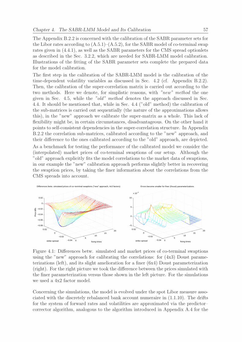
Chapter 4. The SABR-LMM Model and Its Calibration 57
The Appendix B.2.2 is concerned with the calibration of the SABR parameter sets forthe Libor rates according to (A.5.1)–(A.5.2), for the SABR model of co-terminal swaprates given in (4.4.1), as well as the SABR parameters for the CMS spread optionletsas described in the Sec. 3.2.2, which are needed for SABR-LMM model calibration.Illustrations of the fitting of the SABR parameter sets complete the prepared datafor the model calibration.
The first step in the calibration of the SABR-LMM model is the calibration of thetime-dependent volatility variables as discussed in Sec. 4.2 (cf. Appendix B.2.2).Then, the calibration of the super-correlation matrix is carried out according to thetwo methods. Here we denote, for simplistic reasons, with ”new” method the onegiven in Sec. 4.5, while the ”old” method denotes the approach discussed in Sec.4.4. It should be mentioned that, while in Sec. 4.4 (”old” method) the calibration ofthe sub-matrices is carried out sequentially (the nature of the approximations allowsthis), in the ”new” approach we calibrate the super-matrix as a whole. This lack offlexibility might be, in certain circumstances, disadvantageous. On the other hand itpoints to self-consistent dependencies in the super-correlation structure. In AppendixB.2.2 the correlation sub-matrices, calibrated according to the ”new” approach, andtheir difference to the ones calibrated according to the ”old” approach, are depicted.
As a benchmark for testing the performance of the calibrated model we consider the(interpolated) market prices of co-terminal swaptions of our setup. Although the”old” approach explicitly fits the model correlations to the market data of swaptions,in our example the ”new” calibration approach performs slightly better in recoveringthe swaption prices, by taking the finer information about the correlations from theCMS spreads into account.
05
1015
20
−0.04
−0.02
0
0.02
−0.08
−0.06
−0.04
−0.02
0
0.02
fixing times
Differences betw. simulated prices of co−terminal swaptions ("new" approach, 4x3 factors)
strike spread
Pric
e di
ffs
05
1015
20
−0.04
−0.02
0
0.02
−5
0
5
10
x 10−4
fixing times
Errors become smaller for finer (Doust) parameterizations
strike spread
Figure 4.1: Differences betw. simulated and market prices of co-terminal swaptionsusing the ”new” approach for calibrating the correlations: for (4x3) Doust parame-terizations (left), and its slight amelioration for a finer (6x4) Doust parameterization(right). For the right picture we took the difference between the prices simulated withthe finer parameterization versus those shown in the left picture. For the simulationswe used a 4x2 factor model.
Concerning the simulations, the model is evolved under the spot Libor measure asso-ciated with the discretely rebalanced bank account numeraire in (1.1.10). The driftsfor the system of forward rates and volatilities are approximated via the predictor–corrector algorithm, analogous to the algorithm introduced in Appendix A.4 for the

Chapter 4. The SABR-LMM Model and Its Calibration 58
0
5
10
15
20
−0.04−0.02
00.02
−5
0
5
10
x 10−4
fixing times
Comparison betw. the two approaches (4x3 factors)
strike spread0
510
1520
−0.04
−0.02
0
0.02
−5
0
5
10
x 10−4
fixing times
Comparison betw. the two approaches (3x1 factors)
strike spread
Figure 4.2: These two pictures show the performance of the ”new” method vs. the”old” one (the parts above zero show the better performance of the ”new” method)for different factorizations. In the left picture the simulations were performed with a4x2 factor model, while in the right picture a 3x1 factor model was taken. For thecorrelations we used a (4x3)-Doust parameterization for both cases.
LMM. For the simulations we used different number of stochastic factors for theforward rates and their volatilities7, and made use of the spectral decomposition dis-cussed in Sec. 1.3.3 for the correlation matrices. In all the runs the number of MonteCarlo simulations was 20.000.
In the Fig. 4.1 the difference between simulated and market prices of co-terminalswaptions using the ”new” approach is shown. The performance of a (4x3) Doust pa-rameterization (left) and a finer (6x4) Doust parameterization (right) are compared.The finer parameterization performs slightly better (right-hand picture). This ame-lioration, though, is very small, and can be interpreted as an evidence for the effec-tiveness and robustness of the method8.
The pictures in Fig. 4.2 shall illustrate the performance of the two methods of cal-ibrating the correlations for different factorizations, i.e. different number of modelstochastic drivers. They show the difference between the simulated swaption priceswith the ”new” correlation calibration method against the ones simulated with cor-relations calibrated according to the ”old” method.
We shall identify three effects out of these pictures: the first is that for long-termexpiries there is (almost) no difference between the two methods, i.e. they are equallygood performing. This fact can easily be explained with the ”freezing” of swapweights which has been applied to the derivation of both approaches. The secondeffect is that, although in a very small scale, the ”new” approach apparently providesa slightly smaller error between the simulated and market prices of swaptions (thepositive parts of the surface). Finally, with increasing the number of stochasticdrivers, i.e. retrieving more information from the correlation matrices via the useddecomposition, the model errors become smaller; an evidence more of the importanceof the information stored in the correlation structure.
7It is a rather standard market usance that in the simulations the number of factors for volatilities(in the stochastic volatility models) is smaller than the one for the Libor rates, attributing ”lessimportance” to the volatility sub-model.
8For a better proof one would need to have data enough to be able to sketch the dependence ofthe degree of parameterization fineness on the simulation error.

Chapter 5
Conclusion andOutlook
In this work we have developed and discussed a novel approach of calibrating the richcorrelation structure in the SABR-LMM model of forward rates, implying marketinformation on correlations from correlation-sensitive derivatives such as CMS spreadoptions, which additionally incorporate information on the swap rate correlations. Tothis end the derivation of analytical pricing formulas for these products is necessary.
Applying the effective Markovian projection (MP) technique we have derived a displa-ced–diffusion SABR model for the spread between the swap rates with different ma-turities. Consequently, we can apply the seminal formula of Hagan et al. to calibratethe SABR model parameters for the CMS spread to the market implied (normal)volatilities of the CMS spread options. For the ATM values in the payoff measureof the projected SDE we have used a standard smile-consistent replication of thenecessary convexity adjustment with swaptions. In this way we are able to retrievethe additional information about the swap rate correlations from the whole marketsmile of CMS spread options and embed it into the SABR-LMM model correlations.
Numerical simulations with different parameterizations of the correlation sub-matriceshave evidenced effectiveness and robustness of this calibration approach. Simulationswith real market data have shown so far a slightly better performance, (even) in termsof pricing errors of swaptions, of this approach in comparison to the rather standardone of calibrating the model correlations to swaptions’ implied volatilities. As ex-pected, the used ”freezing” of the swap rate coefficients turns out to be restrictive forthe usage of this method for longer expiries. This is a drawback in both approaches.
Nevertheless, the simulations were based only on a snapshot of market data, suchthat further numerical analysis is certainly necessary to study the properties of thisapproach for different market movements and different constellations of volatilityskews/smiles of the market segments involved before it can be used in practice. Themarket data involved in the proposed calibration is very broad and these empiricalstudies would have gone far beyond the scope of this project. Also not presented inthis thesis is a performance analysis on the valuation of more complex correlation-sensitive products. Future research should also encompass the parameterizations andthe interplay of the different sub-matrices of the model correlation structure, takingalso an weighting of the sub-matrices into account for the calibration. A comparisonto other stochastic volatility models which use the MP technique for their calibration,such as e.g. SV-LMM and FLTSS-LMM, may also be objective for studies and futuredevelopments in this area, particularly regarding the MP technique.
59
Appendix A
Classical Models andSABR-LMM
A.1 Valuation in LMM
With regard to the scope of this work, this section is concerned with the analyt-ical pricing of basic benchmark instruments which are used to calibrate the LMM(and partly also the SABR-LMM). The notation chosen for the different financialinstruments is aligned with the notation used in Brigo-Mercurio [2007].
Forward rates and FRAs
An alternative definition of the forward rate is given in the literature (cf. Brigo-Mercurio [2007]) also through a Forward Rate Agreement (FRA). A FRA is a contractgiving its holder an interest rate payment for the period between two time instants,T and S, with T < S. At the maturity S, a fixed payment based on a fixed rate K isexchanged against a floating payment based on the spot rate F (T, T, S), resetting inT with maturity S. Basically, this contract allows to lock in the interest rate betweenT and S at a desired value K. The payoff of this contract at S is given by
τ(T, S)(K − F (T, T, S)),
where the notional involved is taken to be one, and for the sake of simplicity, bothrates are assumed to have the same day count conventions. A time t ≤ T this contractwill have the price
FRA(t, T, S,K) = B(t.S)ESt [τ(T, S) (K − F (T, T, S))](A.1.1)
= τ(T, S)B(t.S) (K − F (t, T, S)) ,
with respect to its natural measure PS, which corresponds to the numeraire B(t, S).
To render this contract fair (i.e. at value zero) at time t, K has to be equal tothe forward Libor rate F (t, T, S). Thus, its ”fairness” can be invoked to define theforward Libor rates. Here, and in the sequel, we assume a notional of one for thecontracts we shall present1.
1Any other notional N ∈ R is simply a multiplicator to the price of the financial contract. It isassumed to have been fixed at the beginning of the contract and remain constant over time.
60

Appendix A. Classical Models and SABR-LMM 61
Interest rate swaps
A generalization of the FRA is the interest rate swap. An interest rate (forwardstarting payer) swap (IRS) on a loan over a period [Tm, Tn], with notional amount 1,is a two-legs contract, starting from a future time instant Tm, to pay a fixed rate Kand to receive spot Libor (floating) at the payment dates Tm+1, ..., Tn. At every timeTi ∈ Tm+1, ..., Tn the fixed leg pays out τi−1K, whereas the floating leg pays theamount τi−1Fi−1(Ti), corresponding to the interest rate Fi, resetting at the previoustime Ti−1
2. The IRS paying the fixed leg and receiving the floating leg is termed payerIRS (IRSp), whereas the opposite case is termed receiver IRS (IRSr). We assumeagain a notional of one in the sequel.
The value of a receiver IRS at time t is given by (cf. Brigo-Mercurio [2007])
IRSr(t, Tm, Tn) =n∑
i=m+1
FRA(t, Ti−1, Ti, K) =n∑
i=m+1
τi−1B(t, Ti) (K − Fi−1(t))
= B(t, Tn)−B(t, Tm) +n∑
i=m+1
τi−1B(t, Ti)K.
Making the contract ”fair” at time t, (i.e. setting IRSr(t, Tm, Tn) = 0) leads to thedefinition of the swap rate K as(A.1.2)
K := Sm,n(t) =B(t, Tm)− B(t, Tn)∑n
i=m+1 τi−1B(t, Ti)=
B(t, Tm)−B(t, Tn)
Bm,n(t), t ∈ [0, Tm].
The amount Bm,n(t) :=∑n
i=m+1 τi−1B(t, Ti) is called the swap annuity and representsa natural numeraire for the swap rate process3.
Similarly to caps and floors introduced in the next section, IRS contracts may besettled in arrears or, as assumed above, in advance.
Caps and Floors
A caplet/floorlet is a contract that can be viewed as a payer/receiver FRA whereexchange payment is executed only if it has a positive value. The payoff profile of acaplet with strike level κ at reset time T and settlement time S reads
B(T, S)(
FRA(T, T, S, κ))+
= B(T, S)τ(T, S)(
F (T, T, S)− κ)+
,
leading to the pricing formula at t ≤ T < S:
CPL(t, T, S, κ) = B(t, S)τ(T, S)ESt
[
(
F (T, T, S)− κ)+]
= B(t, S)τ(T, S)BS(
F (t, T, S), κ, σBlack
T (κ)√T − t, 1
)
,(A.1.3)
2It is obvious to state that in general Fi(t) ≡ Fi(Ti), for any t ≥ Ti.3We refer to (A.1.2) as the standard swap rate. In practice, however, there are several con-
stellations of a swap contract, depending on the market practice, day count conventions, paymentfrequencies etc., which, in fact, do not impact the theory. The generalization to these constellationsis straightforward such that we will consider only the simplified version in this work.

Appendix A. Classical Models and SABR-LMM 62
where the expectation is taken with respect to the forward measure related to B(t, S).The quantity σBlack
T (κ) denotes the implied (Black-) volatility, as seen from time t, ofthe caplet with strike κ in the Black–framework, i.e. as if the underlying forwardrate F (t, T, S) was following the Black-Scholes lognormal dynamics.
In the LMM introduced in Section 1.1 the price of the at–the–money (ATM) caplet,for instance, is obtained by putting κ = F (t, T, S) in (A.1.3). The ATM impliedBlack-volatility σBlack
T = σBlack
T (F (t, T, S))4 and the model volatility γ(t, T, S) have tosatisfy the relation
(A.1.4) (σBlack
T )2 (T − t) =
∫ T
t
‖γ(u, T, S)‖2 du5.
BS denotes the known Black-Scholes formula6, firstly introduced in the seminal workof Black-Scholes [1973], and given by the equation
BS(
F,K, σ, ω)
= FωΦ(ωd+(F,K, σ))−KωΦ(ωd−(F,K, σ)),(A.1.5)
d±(F,K, σ)) =ln(F/K)± σ2/2
σ, ω = +/− 1 (call/put),(A.1.6)
where Φ denotes the standard Gaussian cumulative distribution function.
Analogously to (A.1.3), the pricing equation for the corresponding floorlet with thesame strike κ reads
(A.1.7) FLL(t, T, S, κ) = B(t, S)τ(T, S)BS(
F (t, T, S), κ, σBlack
T (κ)√T − t,−1
)
.
We mention here that at time t a caplet7 is at–the–money/out–of–the–money/in–the–money when its strike κ = F (t, T, S) / κ > F (t, T, S) / κ < F (t, T, S).
A interest rate cap (CAP) is a contract that can be viewed as a payer IRS where eachexchange payment is executed only if it has a positive value. It can be decomposedadditively in caplets with the same strike level κ, leading to the following pricingformula at time t:
CAP(t, Tm, Tn, κ) =n∑
i=m+1
CPL(t, Ti−1, Ti, κ)
=n∑
i=m+1
B(t, Ti)τi−1BS(
Fi−1(t), κ, σBlack
i−1 (κ)√
Ti−1 − t, 1)
,(A.1.8)
4If not otherwise mentioned or notationally specified the implied Black volatility of an optionwill be an ATM one.
5We see already at this point the severe limitation of the LMM with respect to smile modeling.For caplets with different strikes the model volatility would have to match the equations
(
σBlackT (κ)
)2(T − t) =
∫ T
t
‖γ(u, T, S)‖2 du, ∀ κ.
The impossible task of accurately fitting the whole caplets’ smile surface with a desirable singlevolatility function (cf. Sec 1.3) has led many authors to introduce stochaticity in the model volatility.
6Widely known also as Black-76.7For a floorlet the logic goes analogously.

Appendix A. Classical Models and SABR-LMM 63
with σBlack
i−1 (κ) denoting the implied Black-volatility of the caplet CPL(t, Ti−1, Ti, κ),respectively, as seen at time t. The value for the corresponding interest rate floor(FLO) is analogous.
A CAP(t, Tm, Tn, κ) is said to be at–the–money at time t if and only if Sm,n(t) = κ.It is instead said to be in–the–money when Sm,n(t) > κ and out–of–the–money ifSm,n(t) < κ. For a floor the moneyness is defined analogously.
We see already at this point that while the moneyness for caplets is natural, the onefor cap/floors is rather a market convention. Being ATM for a cap/floor does notnecessarily imply the same property for the caplets it is built upon. We shall cometo this point in Chap. 1.3.2.
A.2 Swap Rate Dynamics and the Choice of Nu-
meraire
Given the swap rate dynamics introduced in Def. 1.3, the commonly used swap ratemodels8 in the literature are the following (cf. Musiela-Rutkowski [2005]):
• the co-terminal swap rate model (cf. Jamshidian [1997], Galluccio et al.[2006]), seen as the more natural model analogous to the forward Libor marketmodel. Within co-terminal SMM for every m = 0, . . . , N − 1 the swap rate
Sm,N(t) =B(t, Tm)−B(t, TN)∑N
i=m+1 τi−1B(t, Ti)=
B(t, Tm)−B(t, TN)
Bm,N(t),
is considered and theBm,N(t)-induced probability measure Pm,N is said to be theco-terminal swap measure for the date Tm if for every k = 0, . . . , N the relativebond price B(t, Tk)/Bm,N (t), t ∈ [0, Tk ∧ Tm] is a local martingale under Pm,N .
• the co-initial swap rate model (cf. Galluccio-Hunter [2003]) where, analogouslyto the co-terminal one, for every m = 1, . . . , N the swap rate S0,m(t), t ≤ T0 isconsidered (fixed starting point). The corresponding probability measure P
0,m
is induced by the numeraire B0,m(t). The demand for the co-initial SMM ismotivated by the desire to value and hedge exotic interest derivatives such asCMS spread options or forward starting swaptions.
• the co-sliding swap rate model (cf. Galluccio et al. [2006]), where we no longerassume that the swap agreements have different lengths but the same startor maturity date. In the co-sliding SMM, on the contrary, the constant lengthK ≥ 1 plays the role of the orientation variable. For everym = 0, . . . , N−K theconsidered swap rates are then given by Sm,m+K(t), t ≤ Tm. The correspondingprobability measure P
m,m+K is induced by Bm,m+K(t). The LMM is the onlyadmissible model of a co-sliding type as it can be seen as a special case of it.
We refer to Galluccio et al. [2006] for their extensive studies on the three typesof swap rate models and their adequateness in practice.
8Discussions about the differences between these models and further modeling issues can be foundin Rebonato [1999b], Brigo-Liinev [2005] and the references therein.

Appendix A. Classical Models and SABR-LMM 64
A.3 Valuation in the Log-Normal Swap Market
Model
The second class of basic derivatives on interest rates is the class of the swap options,or more commonly swaptions. A European (payer) swaption over period [Tm, Tn]gives the right to enter at the future time Tm into an interest rate (payer) swap (IRS)with strike rate κ, starting from Tm. The underlying length Tn − Tm is called thetenor of the swaption. Following Brigo-Mercurio [2007], consider the value of theunderlying payer IRS at swaption expiry time Tm, i.e.
n∑
i=m+1
τi−1B(Tm, Ti)(
Fi−1(Ti−1)− κ)
,
the payoff of the (cash-settled) swaption can be written as
(A.3.1)
(
n∑
i=m+1
τi−1B(Tm, Ti)(
Fi−1(Ti−1)− κ)
)+
= (Sm,n(Tm)− κ)+ Bm,n(Tm),
as the option will be exercised only if the swap value with strike κ is positive. Afundamental difference between the swaptions and the caps can be obviously derivedfrom (A.3.1), this payoff cannot be decomposed in more elementary products, as forthe cap case. As the additive decomposition is not feasible for the (.)+ operator wewill need to consider the joint action of the forward rates involved in the contractpayoff. Due to the convexity of the operator (.)+ the value of a (payer) swaption isalways smaller than the value of the corresponding cap contract.
The market convention is to price swaptions with the Black-Scholes formula. Takingthe natural numeraire given by Bm,n(t), one can price the payoff (A.3.1) with respectto the measure P
m,n by
PSWO(t, Tm, Tn, κ) = Bm,n(t)Em,nt
[
(
Sm,n(Tm)− κ)+]
= Bm,n(t)BS(
Sm,n(t), κ, σBlack
m,n (κ)√
Tm − t, 1)
, t ≤ Tm,(A.3.2)
where the formula for BS is given in (A.1.5)–(A.1.6), Em,nt denotes the expectation
with respect to the probability measure Pm,n, and σBlack
m,n (κ) the implied (Black–)volatility of the swaption quoted in the market.
Within the SMM introduced in Chapter 1.1.4, the ATM Black volatility, σBlack
m,n (Sm,n(t)) =σBlack
m,n , satisfies
(A.3.3)(
σBlack
m,n
)2(Tm − t) =
∫ Tm
t
σm,n(u)2 du.
Analogously, the price for the receiver swaption is given by
RSWO(t, Tm, Tn, κ) = Bm,n(t)Em,nt
[
(
κ− Sm,n(Tm))+]
= Bm,n(t)BS(
Sm,n(t), κ, σBlack
m,n (κ)√
Tm − t,−1)
, t ≤ Tm.(A.3.4)

Appendix A. Classical Models and SABR-LMM 65
A.4 Drift Approximation in LMM and Simulations
As discussed in Chapter 1.1.1, the joint dynamics of forward rates under the ter-minal measure (let say P
k+1 as in (1.1.8)-(1.1.9)) is complex and the correspondingstochastic differential equations are high dimensional and contain state dependentdrift terms. Hence, the joint distributional evolution of forwards in the terminalpricing measure is impossible to be computed explicitly. This leaves two naturalalternatives:
• The naive straightforward alternative is to discretize the corresponding stochas-tic differential equation using some discretization scheme (Euler or Milstein, forexample). After that, using a very small time step it is possible to evolve theforward rates on a fine time grid for the price sensitive events.
• The second alternative is to try to approximate the state dependent stochas-tic integrals by an efficient and accurate method which allows for solving thestochastic differential equation approximately analytically. Then the evolvingthe interest rates over long integration/simulation steps is possible.
The second alternative is more appealing and efficient as for each realization of theforwards only as many steps are needed as there are price sensitive events.
There are several ways to improve the Euler scheme for the numerical integrationof stochastic differential equations. Instead of using any of the well-known explicit,implicit, or standard predictor-corrector methods, here we are going for the hybridtechnique presented in Hunter-Jackel-Joshi [2001]. Hereby we integrate the termsγk(t) · dWk+1
t in (1.1.4) directly as if the drift coefficient is constant over any onetime step. So far this is essentially consistent with the standard Euler method.However, in addition, we account for the indirect stochasticity of the drift term byusing a Predictor-Corrector method. The algorithm for constructing one draw fromthe terminal distribution of the forward rates over one time step reads as follows.
• Evolve the logarithms of the forward rates Fj(t) as if the drifts
µkj (t) :=
−k∑
i=j+1
τiFi(t) σi(t)σj(t)ρi,j(t)
1+τiFi(t), j < k
0 , j = kj∑
i=k+1
τiFi(t) σi(t)σj(t)ρi,j(t)
1+τiFi(t), j > k
.
were constant over [t, t + ∆t), and equal to their initial values at t, accordingto the log-Euler scheme:
log(Fj(t+∆t)) = log(Fj(t)) +√∆tσj(t)
d∑
i=1
bj,izi +
[
µkj (t)−
1
2σj(t)
2
]
∆t,
with the loading vector bj given in (1.1.6)–(1.1.7). z = zi denotes d-independentstandard N (0, 1)-random variables (w.r.t. Pk+1).

Appendix A. Classical Models and SABR-LMM 66
• Compute the drifts at the terminal time with the so evolved forward rates,µkj (t+∆t).
• Average the initially calculated drift coefficients with the newly computed ones:
µkj (t) :=
1
2
(
µkj (t) + µk
j (t+∆t))
.
• Re-evolve Fj(t +∆t) using the same normal variates as initially but using thenew predictor-corrector drift terms µk
j (t).
This is a very natural way to incorporate the drift state-dependence. While furtherand potentially better approximations are possible (cf. Joshi [2003], Joshi-Stacey[2008]), this approach has the advantage of being very simple to understand andimplement, and has been extensively studied with respect to its accuracy (cf. Hunter-Jackel-Joshi [2001]).
A.5 SABR Implied Volatility
The (single) SABR model for the forward rate FT (t) = F (t, T, T ∗) is an extension ofthe CEV model,
(A.5.1) dFT (t) = σT (t)FT (t)βT dW T ∗
t ,
in which 0 ≤ βT ≤ 19 and the volatility parameter σT is assumed to be stochastic,following
(A.5.2) dσT (t) = νTσT (t)dWT ∗
t ,⟨
dW T ∗
t , dW T ∗
t
⟩
= ξTdt.
Except for the normal case of βT = 0 (cf. Hagan-Lesniewski [2001]), no explicitsolution to this model is known. The general case can be solved approximately bymeans of an asymptotic expansion of (A.5.1)-(A.5.2) in the parameter ǫ = νT
√T . In
what follows the initial state is given by FT (0) and σT (0). In the sequel the SABRinitial volatility parameter σT (0) will be denoted as
σSABR
T := σT (0).
Following the seminal work Hagan et al. [2002], we write t = Ts, and define X(s) =FT (Ts), Y (s) = σT (Ts)/νT such that the SABR dynamics can be recast in the form
dX(s) = ǫY (s)X(s)βT dW T ∗
s ,
dY (s) = ǫY (s)dW T ∗
s ,
where we have also used the well known scaling law W T ∗
Ts =√TW T ∗
s for Brownianmotions. The initial conditions take the shape
X(0) = FT (0), Y (0) = σSABR
T /νT .
9We note that, according to Jourdain [2004], if βT = 1 and the rate-volatility correlationparameter ξT > 0, then the process FT (t), while a local martingale, fails to be a martingale in P
T∗
.

Appendix A. Classical Models and SABR-LMM 67
Under typical market conditions, the parameter ǫ is small, and the asymptotic solu-tion is quite accurate and easy implementable in computer code. As a consequence,the asymptotic solution to the SABR model lends itself well to valuation and riskmanagement of large portfolios of options in real time. In order to describe theasymptotic solution, we denote with
σNorm
T (K) ≈ σNorm(T,K, FT (0), σSABR
T , νT , βT , ξT ) =: σNorm
T
the implied normal volatility of an option struck at K and expiring T years from now(i.e. t = 0). The analysis of Hagan et al. [2002] of the model dynamics shows thatthe implied normal volatility is approximately given by:
σNorm
T = σSABR
T (FT (0)K)βT /2 1 + 124log2(FT (0)/K) + 1
1920log4(FT (0)/K) + ...
1 + (1−βT )2
24log2(FT (0)/K) + (1−βT )4
1920log4(FT (0)/K) + ...
·(
ζ
δ(ζ)
)
·
1 +
[−βT (2− βT )(σSABR
T )2
24(FT (0)K)1−βT+
ξTνTσSABR
T βT
4(FT (0)K)(1−βT )/2+
2− 3ξ2T24
ν2T
]
T + ...
.
The distance function entering the formula above is given by:(A.5.3)
ζ =νT
σSABR
T
(FT (0)K)(1−βT )/2 log(FT (0)/K), δ(ζ) = log
(
√
1− 2ζξT + ζ2 − ξT + ζ
1− ξT
)
.
Hagan et al. [2002] describes how to approximatively obtain the implied lognormalvolatility for Black’s model
σBlack
T (K) ≈ σBlack(T,K, FT (0), σSABR
T , νT , βT , ξT ) =: σBlack
T
by giving the following relationship to the normal volatility:
(A.5.4) σNorm
T =σBlack
T (FT (0)−K)
log(FT (0)/K)
1− 1
24(σBlack
T )2T + . . .
.
Hence, the approximated implied Black volatility for the SABR model of an optionstruck on FT at K, expiring at T, reads then
σBlack
T =σSABR
T
(FT (0)K)(1−βT )/2(
1 + (1−βT )2
24log2(FT (0)/K) + (1−βT )4
1920log4(FT (0)/K) + ...
)
·(
ζ
δ(ζ)
)
·
1 +
[
(1− βT )2(σSABR
T )2
24(FT (0)K)1−βT+
ξTνTσSABR
T βT
4(FT (0)K)(1−βT )/2+
2− 3ξ2T24
ν2T
]
T + ...
.
Remark A.1 Given the analogous SABR model for the swap rate Sm,n as in (4.4.1),the approximative implied SABR volatility of a swaption on the swap rate Sm,n, withtenor (Tn − Tm) and strike K reads
(A.5.5) σBlack
m,n (K) ≈ σBlack(Tm, K, Sm,n(0), σSABR
m,n , νm,n, βm,n, ξm,n).
It is obvious to mention that the approximative formula for the SABR implied volatil-ity can be extended to the SABR model of any underlying. In Sec. 3.2.2 we will seean application of this formula for the SABR model of a CMS swap spread.

Appendix A. Classical Models and SABR-LMM 68
For practical use in interest rate options portfolio management, an important step isthe calibration of the model parameters. For each benchmark option expiry and un-derlying tenor we have to calibrate four model parameters: σSABR
T , νT , βT , ξT . In orderto do it we need market implied volatilities for several different strikes. The experi-ence shows (cf. Rebonato-McKay-White [2009]) that there is a bit of redundancybetween the parameters βT and ξT . As a result, one usually calibrates the model byfixing one of these parameters.
Two common practices are:
(a) Fix βT , say βT = 0.5, and calibrate σSABR
T , νT , ξT .
(b) Fix ξT = 0, and calibrate σSABR
T , νT , βT .
Calibration results show a persistent term structure of the model parameters as func-tions of the expiration and underlying tenor. Typical is the shape of the parameterνT which start out high for short dated options and then declines monotonically asthe option expiration increases. This indicates presumably that modeling short datedoptions should include a jump diffusion component (cf. Hagan-Lesniewski [2008]),an ongoing research topic. A good empirical analysis of the SABR parameters canbe found in Rebonato-McKay-White [2009].
Special Cases.
Two cases are worthy of special treatment: the stochastic normal model (βT = 0)and the stochastic lognormal model (βT = 1). Both these models are simple enoughthat the expansion can be continued. For the stochastic normal model (βT = 0) theapproximative implied volatilities of European calls and puts are:
σNorm
T = σSABR
T
[
1 +2− 3ξT
24ν2TT + . . .
]
,
σBlack
T = σSABR
T
log(FT (0)/K)
FT (0)−K·(
ζ
δ(ζ)
)
·
1 +
[
(σSABR
T )2
24FT (0)K+
2− 3ξ2T24
ν2T
]
T + . . .
,
ζ =νT
σSABR
T
√
FT (0)K log(FT (0)/K), δ(ζ) = log
(
√
1− 2ζξT + ζ2 − ξT + ζ
1− ξT
)
.
For the stochastic log normal model (βT = 1) the approximative implied volatilitiesare:
σNorm
T = σSABR
T
FT (0)−K
log(FT (0)/K)·(
ζ
δ(ζ)
)
·
1 +
[−(σSABR
T )2
24+
ξTνTσSABR
T
4+
2− 3ξ2T24
ν2T
]
T + . . .
,
σBlack
T = σSABR
T
(
ζ
δ(ζ)
)
·
1 +
[
νTσSABR
T ξT4
+2− 3ξ2T
24ν2T
]
T + . . .
,
ζ =νT
σSABR
T
log(FT (0)/K), δ(ζ) = log
(
√
1− 2ζξT + ζ2 − ξT + ζ
1− ξT
)
.

Appendix B
Calibration Details
B.1 Bootstrapping the Market Data
Here we describe the general setup, the original and the pre-processed market data.Thetime horizon chosen for our model setup is 20 years ahead with an equidistant 6months (6M) time grid. The market data are taken from Thomson Reuters c© asof September 12, 2011. The implementation has been carried out in C++ usingQuantLib1. The raw market data and the interpolated data to be input to the mod-els are given as follows.
• The yield curve:
– Market data: EUR/EURIB yield curve consisting of deposit rates, futuresand swap rates;
– Interpolated market quotes: set of 6M contiguous forward rates rolled for20 years ahead. The discount term structure has been bootstrapped fromthe yield term structure and log-linearly interpolated2, see Fig. B.1.
0 5 10 15 200
0.005
0.01
0.015
0.02
0.025
0.03
0.035
0.04
0.045
0.05
fixing times
forw
ards
Forward rates
0 5 10 15 200
0.005
0.01
0.015
0.02
0.025
0.03
0.035
0.04
0.045
0.05
fixing times
co−t
erm
sw
ap ra
tes
Forward co−terminal swap rates
Figure B.1: Model Libor and swap rates: 6M contiguous forward Libor rates forthe time horizon of 20 years and the corresponding grid of co-terminal swap ratesbootstrapped from market data as of Sept. 12, 2011.
1QuantLib Library Version 1.0.1., to be found in http://quantlib.org.2Day count convention (DC) = Actual365Fixed, business days (BD) = ”Modified Following”.
69

Appendix B. Calibration Details 70
• The caps/floors market:
– Market data: EUR/EURIB ATM 6M cap/floor (implied) volatility quotesand a matrix of 6M cap/floor smile spreads3 for strike spreads over ATMranging within [-3%, +5%] and different expiries up to 30 years ahead;
– Interpolated quotes: 6M grid of contiguous 6M ATM caplet series fillingthe 20 years time horizon. The resulting caplet volatility surface overstrikes and expiries uses bi-cubic spline interpolation, see Fig. B.2.
0
5
10
15
20
−0.02
0
0.02
0.04
0
0.5
1
1.5
fixing times
Caplets smile
strike spread
impl
. vol
0
5
10
15
20
−0.02
0
0.02
0.04
0
0.005
0.01
0.015
fixing times
Caplets prices
strike spread
capl
et p
rices
Figure B.2: Model caplets: grid of implied volatilities and Black-prices of contiguous6M caplet series rolled 20 years ahead for the given strikes, interpolated from themarket data as of Sept. 12, 2011.
• The swaption volatilities:
– Market data: EUR/EURIB ATM swaption volatilities for tenors from 1Yto 30Y, for different expiries up to 30 years ahead; EUR/EURIB swaptionsmile spreads for the strike spreads over ATM ranging in [-4%, +5%], andfor tenors up to 30 years and expiries up to 20 years ahead;
– Interpolated quotes: 6M spaced series of co-terminal swaps for the 20 yearsmodel time horizon, with 6M fixing and floating legs; ATM volatilities forthe co-terminal swaps built by means of bilinear interpolation from themarket data; series of 6M–expiring swaptions with the co-terminal swapsas underlyings, for each given absolute strike; resulting in a surface ofabsolute swaption volatilities with the axis (expiry × strike), see Fig. B.3.
• CMS Spread Optionlets4:
– Market data: implied ATM normal volatilities for the Single Look option-lets on the EUR/EURIB CMS spreads 10Y/2Y, 30Y/2Y and 30Y/10Yfor different expiries from 2 weeks up to 20 years ahead; additionally nor-mal volatility smile spreads (in basis points (bp)) for the mentioned CMSspread optionlets with the absolute strike range [-0.5%, +1.5%] and ex-piries up to 20 years ahead;
3The cap/floor volatility smile is given in terms of vol spreads over the ATM volas.4We thank Dr. Jorg Kienitz for providing the CMS spread options data used for the calibration
examples in this chapter.

Appendix B. Calibration Details 71
0
5
1015
20
−0.04
−0.02
0
0.02
0.2
0.4
0.6
0.8
1
fixing times
Swaptions smile
strike spread
impl
vol
0
5
10
15
20
−0.04
−0.02
0
0.02
0
0.1
0.2
0.3
0.4
0.5
fixing times
Swaptions prices
strike spread
Sw
aptio
n pr
ices
Figure B.3: Model swaptions: grid of implied volatilities and Black-prices of swap-tions on co-terminal swaps with 6M stepping expiries, interpolated from the marketdata as of Sept. 12, 2011.
– Interpolated quotes: normal volatility smile in bp of CMS spread optionletson 10Y/2Y, 20Y/2Y and 20Y/10Y on a 6M grid of expiries, given in TableB.1, built by using 2D-interpolation.
B.2 Parameterization of SABR–LMM and Its Cal-
ibration
B.2.1 Parameterization of the SABR–LMM Model
Starting from the time-homogeneous SABR–LMM model, given in Def. 4.1, we shalluse the following parameterization of the model variables:
• For the forward rate volatility we will use the parameterization (4.2.1) with thetime-homog. function g given in (4.2.2).
• For the volatility of volatility function h we again will use a time-homog. pa-rameterization given in (4.2.5).
• For the super–correlation matrix (4.3.1) we will use full-rank mixed parameter-izationsas follows:
– Doust’s correlation parametrization for the forward rate – forward ratesubmatrix, given in (1.3.14);
– Doust’s parametrization for the volatility – volatility correlations, given(1.3.14), or alternatively, the two-parameter exponential parameterizationgiven in (1.3.9);
– The parametrization given in Example 4.3 (4.3.4) for the correlations be-tween the forward rates and the volatilities.

Appendix B. Calibration Details 72
10Y/2Y ATM rate -0.5% -0.25% 0% 0.25% 0.5% 0.75% 1.0% 1.5%
6M 0.0117850 2 2 2 27 21 14 9 31Y 0.0123250 33 33 33 109 91 74 59 40
1Y6M 0.0114528 63 64 64 189 159 132 107 752Y 0.0109419 96 97 98 269 229 191 158 114
2Y6M 0.0096187 133 134 135 347 297 250 209 1543Y 0.0082777 173 176 178 424 364 308 260 198
3Y6M 0.0073985 216 219 221 495 426 363 310 2404Y 0.0065000 262 266 269 567 489 420 361 285
4Y6M 0.0061953 311 316 320 638 553 476 413 3325Y 0.0059208 362 369 374 711 618 535 467 381
5Y6M 0.0059321 416 424 430 785 685 596 523 4316Y 0.0059784 472 482 489 861 753 659 582 484
6Y6M 0.0060139 529 540 549 938 823 723 641 5387Y 0.0060692 590 602 612 1018 896 790 704 595
7Y6M 0.0061427 650 664 675 1098 970 858 767 6528Y 0.0063303 714 729 741 1181 1046 928 833 712
8Y6M 0.0063114 779 796 809 1264 1122 999 899 7739Y 0.0064165 848 866 880 1349 1200 1072 968 836
9Y6M 0.0064623 916 936 951 1430 1276 1143 1035 89810Y 0.0066037 989 1010 1026 1514 1354 1216 1105 963
10Y6M 0.0067320 1063 1085 1103 1596 1431 1289 1174 1028
20Y/2Y ATM rate -0.5% -0.25% 0% 0.25% 0.5% 0.75% 1.0% 1.5%
6M 0.0158146 4.59 4.34 4.35 3.96 33.69 26.93 20.30 9.61
20Y/10Y ATM rate -0.5% -0.25% 0% 0.25% 0.5% 0.75% 1.0% 1.5
6M 0.0040295 1.08 1.24 1.25 4.39 1.12 0.21 0.37 0.84
Table B.1: Interpolated 10Y/2Y, 20Y/2Y, 20Y/10Y CMS spread volatility smile (inbp) for the different strikes (first row), and the calculated ATM spread rates on the6M grid of expiries (first left column) within the model time horizon, based on dataas of Sept. 12, 2011.
B.2.2 Calibration Procedure
The calibration starts with bootstrapping and preprocessing the market data to fita predefined (6M)-equidistantly spaced time grid, 0, T0, ..., TN, (TN−1 = 20Y, thelast fixing date) of model forward rates and co-terminal swaps, briefly described inAppendix B.1. Then, the following calibration steps have to be carried out:
The Calibration of the SABR Forward and Swap Rate Parameters
As the next step we have to calibrate the (auxiliary) SABR models for the forward((A.5.1)– (A.5.2)) and swap rates (4.4.1) separately, by using the formulas in Ap-pendix A.5 which can be split in the following steps:
• Calibration of the time-homogeneous SABR model of forward rates Fi, i ∈

Appendix B. Calibration Details 73
0, ..., N − 1, as defined in ((A.5.1)– (A.5.2)). The βi parameters are set tothe constant βi ≡ β = 0.5, throughoutly. The calibration consists of optimizingover the SABR parameters, σSABR
i , νi and ξi, by using the Levenberg-Marquardtalgorithm (cf. (4.1.1)):
(B.2.1) minσSABRi ,νi,ξi
∑
K
[
σBlack(Ti, K, Fi(0), σSABR
i , νi, 0.5, ξi)− σBlack
i (K)
]2
,
where the sum is taken over the available strikes K, σBlack
i (K) is the (inter-polated) market implied caplet volatility at strike K, and the SABR impliedvolatility σBlack is given in Chap. A.5. The goodness of the fit of the forwardrate SABR parameters is illustrated in the Fig. B.4 (left picture).
0
5
10
15
20
−0.02
0
0.02
0.04
0
0.01
0.02
0.03
0.04
fixing times
SABR fitting to caplets prices
strike spread
rel.
diffs
0
5
10
15
20
−0.04
−0.02
0
0.02
0
0.02
0.04
0.06
0.08
fixing times
SABR fitting to swaptions prices
strike spread
rel.
diffs
Figure B.4: Relative errors to market Black-prices of model caplets (left) and co-term.swaptions (right) of the prices calculated using the calibrated SABR parameters.
• Calibration of the SABR dynamics for the co-terminal swap rate Si,N , i ∈0, . . . , N − 1, as given in (4.4.1). We again make use of the Levenberg-Marquardt algorithm to calibrate the SABR parameter for the grid of co-terminal swaps, where again the exponent βi,N ≡ 1/2 is kept constant andthe other three parameters, σSABR
i,N , νi,N and ξi,N , are calibrated to match thebootstrapped swaption smile,
minσSABRi,N
,νi,N ,ξi,N
∑
κ
[
σBlack(Ti, κ, Si,N (0), σSABR
i,N , νi,N , 0.5, ξi,N )− σBlack
i,N (κ)
]2
,
with κ representing the available swaption strikes, σBlack
i,N (κ) the market impliedswaption volatility at strike κ, and the SABR implied volatility σBlack given inChap. A.5. The fit of the SABR parameters for the swap rates is illustrated inthe Fig. B.4 (right picture).
• Calibration of the SABR-DD dynamics (cf. (3.2.39)) of the CMS spreadsSk,n1,n2
, k ∈ 0, . . . ,maxn1, n2 − 1, to the given implied (normal) volatil-ity smile given in Tab. B.1, by using the formulae in Sec. A.5, together withHagan [2003] replication approach (3.2.46) for the expectation of the spreadin the corrsp. forward measure. The determination of the SABR parame-ters, Γk,n1,n2
, Υk,n1,n2and qk,n1,n2
, (βk,n1,n2= 1), is done by using the standard
Levenberg-Marquardt optimization algorithm.

Appendix B. Calibration Details 74
The following Fig. B.5 shows the fitting of the SABR parameters for the CMSspread 10Y/2Y, i.e. the difference between the normal volatilities calculatedwith the calibrated SABR parameters and the market volatilities given in TableB.1. It should be mentioned that the fitting implicitly includes the approxima-tion errors of the Hagan’s convexity adjustment method in (3.2.46).
0
2
4
6
8
10
−5
0
5
10
15
x 10−3
0
0.02
0.04
0.06
0.08
fixing times
Smile fitting of the CMS Spread 10y − 2y
strike
Figure B.5: Fitting error of the normal volatilities after the calibration of the SABRparameters for the 10Y/2Y CMS spread.
The Calibration of the SABR–LMM Model
Finally, in what follows we describe briefly the calibration of the time-homogeneousSABR-LMM for the forward rates, as given in Def. 4.1.
• To calibrate the forward rate volatility in the SABR–LMM model we follow theapproach discussed in Chap. 4.2, by using the parameterization given in Sec.B.2.1. To this end we should
– perform (4.2.3) to calibrate the time-homogeneous function g and adjustthe initial rate-dependent values ki(0) according to (4.2.4);
– calibrate the function h as in (4.2.6), by taking the restriction (4.2.8) intoaccount.
• Using the full-factor parameterizations introduced in Sec. B.2.1, the calibrationof the super–correlation matrix is carried out in the following two different ways:
– Given the calibrated SABR parameters for the swap rate dynamics (cf.(4.4.1)), we follow the approach given in Chap. 4.4 (”old” approach),where the correlation submatrices of (4.3.1) are successively calibratedaccording to the equations (4.4.4)–(4.4.7);
– Following the (”new”) approach in Chap. 4.5, we use the determinedSABR-DD parameters for the CMS spreads to derive via (3.2.41)–(3.2.44)the parameters of the super–correlation matrix.
In both cases we use square differences between the model parameters and thetarget values as objective function and apply the Levenberg-Marquardt opti-mization algorithm.

Appendix B. Calibration Details 75
The next Fig. B.6 - B.8 show the correlation sub-matrices, calibrated accordingto the ”new” approach, and their difference to the ones calibrated according tothe ”old” approach. As introduced in Sec. B.2.1 we used for these examples aDoust-parameterization of degree M = 3 (4 parameters) for the forward ratecorrelations, and a Doust-parameterization of degree M = 2 (3 parameters)for the volatility correlations. Finally, (4.3.4) is used for the cross correlationsbetween the forward rates and the volatilities.
The pictures show that, while for short-term expiries the correlations betweenthe Libor rates is lower than in the ”old” approach, the other sub-matrices, i.e.vol. - vol. and Libor rate - vol. correlations, generally are higher.
The full picture of the super-correlation matrix (cf. (4.3.1)) is given in the lastFig. B.9, calibrated according to the ”new”-approach.
05
1015
20
0
5
10
15
200
0.2
0.4
0.6
0.8
1
fixing times
Forward Libor rates correlations (new method)
fixing times 05
1015
20
0
5
10
15
20−0.025
−0.02
−0.015
−0.01
−0.005
0
fixing times
Forward Libor rates correlations (diff. betw. "new" and "old" approaches)
fixing times
Figure B.6: Matrix of correlations betw. the Libor rates (left), calibrated to the CMSspread options (”new” approach), and its difference to the corresponding correlationmatrix computed according to Chap. 4.4 (”old” approach).
05
1015
20
05
1015
200
0.2
0.4
0.6
0.8
1
fixing times
Volatility − volatility correlations (new method)
fixing times0
510
1520
0
5
10
15
200
0.002
0.004
0.006
0.008
0.01
fixing times
Volatility − volatility correlations (diff. betw. "new" and "old" approaches)
fixing times
Figure B.7: Matrix of correlations betw. the Libor rate volatilities (left), calibratedto the CMS spread options (”new” approach), and its difference to the correspondingcorrelation matrix computed according to Chap. 4.4 (”old” approach).

Appendix B. Calibration Details 76
0
5
10
15
20
0
5
10
15
20−0.4
−0.3
−0.2
−0.1
0
fixing times
Libor rate − volatility correlations (new method)
fixing times 05
1015
20
0
5
10
15
200
0.05
0.1
0.15
0.2
0.25
fixing times
Libor rate − volatility correlations (diff. betw. "new" and "old" approaches)
fixing times
Figure B.8: Matrix of cross correlations betw. the Libor rates and their volatilities(left), calibrated to the CMS spread options (”new” approach), and its differenceto the corresponding correlation matrix computed according to Chap. 4.4 (”old”approach).
0
20
40
60
80
0
20
40
60
80−0.5
0
0.5
1
Super correlation matrix (new method)
Figure B.9: The full super-correlation matrix (4.3.1), calibrated according to the”new”-approach.

Bibliography
C. Alexander: Common Correlation and Calibrating the Lognormal Forward RateModel. Wilmott Magazine, March 2003, pp. 68-78.
L. Andersen and J. Andreasen: Volatilite Volatilities. Risk, Vol. 15:12 (2002), pp.163–168.
L. Andersen and R. Brotherton-Ratcliffe: Extended Libor Market Models WithStochastic Volatility. Journal of Computational Finance, Vol. 9:1 (2005), pp. 1–40.
L. Andersen and L. Piterbarg: Moment Explosions in Stochastic Volatility Models.Finance and Stochastics, Vol. 11 (2007), pp. 29-50.
A. Antonov and M. Arneguy: Analytical Formulas for Pricing CMS Products in theLibor Market Model with Stochastic Volatility. Working paper, 2009.
A. Antonov and T. Misirpashaev: Markovian Projection Onto a Displaced Diffusion.Generic formulas with applications. International Journal of Theor. and Appl. Fi-nance, Vol. 12:4 (2009), pp. 507–522.
D. Belomestny, A. Kolodko and J. Schoenmakers: Pricing CMS Spread Options in aLibor Market Model. International Journal of Theor. and Appl. Finance, Vol. 13:1(2010), pp. 45–62.
E. Benhamou: A Martingale Result for Convexity Adjustment in the Black PricingModel. Working Paper, 2000.
F. Black: The Pricing of Commodity Contracts. Journal of Financial Economics, Vol.3 (1976), pp. 167-179.
F. Black and M. Scholes: The Pricing of Options and Corporate Liabilities. Journalof Political Economy, Vol. 81:3 (1973), pp. 637-654.
R. H. Borger; J. v. Heys: Calibration of the Libor Market Model Using CorrelationsImplied by CMS Spread Options. Applied Mathematical Finance, Vol 17:5 (2010),pp. 453–469.
A. Brace: Arbitrage-Free Lognormal Interest Rate Models. Risk Seminars, 2nd draft,1997.
A. Brace, D. Gatarek and M. Musiela: The Market Model of Interest Rate Dynamics.Mathematical Finance, Vol. 7:2 (1997), pp. 127–155.
77

BIBLIOGRAPHY 78
D. Brigo, C. Capitani and F. Mercurio: Different Covariance Parametrizations of theLibor Market Model and Joint Caps/Swaptions Calibration. Working paper, 2003.
D. Brigo and J. Liinev: On the Distributional Distance Between the Lognormal LI-BOR and Swap Market Models. Quantitative Finance, Vol. 5:5 (2005), pp. 433-442.
D. Brigo and F. Mercurio: Interest Rate Models - Theory and Practice. With Smile,Inflation and Credit. 2’nd edition. Springer Finance, 2007.
A. Castagna, F. Mercurio and M. Tarenghi: Smile-Consistent CMS Adjustment inClosed Form: Introducing the Vanna-Volga Approach. Working paper, 2007.
R. Cont and P. Tankov: Financial Modelling for Jump Processes. Chapman and Hall,2004.
J. Cox: Notes on Option Pricing I: Constant Clasticity of Variance Diffusions. Jour-nal of Portfolio Management, Vol. 22 (1996), pp. 15-17.
J. C. Cox, J. E. Ingersoll and S. A. Ross: A Theory of the Term Structure of InterestRates. Econometrica, Vol. 53 (1985), pp. 385-407.
P. Doust: Modelling Discrete Probabilities. Working paper, 2007.
B. Dupire: Pricing with a smile. Risk, Vol. 7:1 (1994), pp. 18–20.
B. Dupire: A Unified Theory of Volatility. Working Paper, 1994.
S. Galluccio, J.-M. Ly, Z. Huang and O. Scaillet: Theory and Calibration of SwapMarket Models. Mathematical Finance, Vol. 17:1 (2006), pp. 111–141.
S. Galluccio and C. Hunter: The Co-Initial Swap Market Model. Working paper,2003.
D. Gatarek, P. Bachert and R. Maksymiuk: The LIBOR Market Model in Practice.Wiley Finance, 2006.
H. Geman, N. El Karoui, J.C. Rochet: Changes of Numeraire, Changes of ProbabilityMeasure and Option Pricing. Journal of Applied Probability, Vol. 32:2 (1995), pp.443–458.
P. Glasserman: Monte Carlo Methods in Financial Engineering. Springer, Berlin,2003.
I. Gyoengy: Mimicking the One-Dimensional Marginal Distributions of ProcessesHaving an Ito Differential. Probability Theory and Related Fields, Vol. 71 (1986),pp. 501–516.
P. Hagan, A. Lesniewski and D.E. Woodward: Probability Distribution in the SABRModel of Stochastic Volatility. Working paper, 2001.
P. S. Hagan: Convexity conundrums: Pricing CMS Swaps, Caps and Floors. WilmottMagazine, March 2003, pp. 38–44.

BIBLIOGRAPHY 79
P. S. Hagan and M. Konikov: Interest Rate Volatility Cube: Construction and Use.Working paper, 2004.
P. S. Hagan, D. Kumar, A. Lesniewski and D. E. Woodward: Managing Smile Risk.Wilmott Magazine, September 2002, pp. 84–108.
P. Hagan and A. Lesniewski: LIBOR Market Model With SABR Style StochasticVvolatility Models. Working paper, 2008.
D. Heath, R. Jarrow and A. Morton: Bond Pricing and the Term Structure of InterestRates: A New Methodology for Contingent Claims Valuation. Econometrica, Vol60 (1992), pp. 77–105.
J. C. Hull: Options, Futures and Other Derivatives. 6’th edition. Prentice Hall, 2005.
J. C. Hull and A. White: Efficient Procedures for Valuing European and AmericanPath Dependent Options. Journal of Derivatives, Vol. 1 (1993), 21–31.
J. C. Hull and A. White: Forward Rate Volatilities, Swap Rate Volatilities, and theImplementation of the Libor Market Model. Journal of Fixed Income, Vol. 10:2(2000), pp. 46-62.
P. J. Hunt and J. E. Kennedy: Financial Derivatives in Theory and Practice. WileyFinance, 2004.
P. J. Hunt and A. Pelsser: Arbitrage-Free Pricing of Quanto-Swaptions. Journal ofFinancial Engineering, Vol. 7:1 (1998), pp. 25–33.
C. J. Hunter, P. Jackel and M. S. Joshi: Drift Approximations in a Forward-Rate-Based LIBOR Market Model. Published as Getting the Drift, Risk, July 2001, pp.81-84.
F. Jamshidian: LIBOR and Swap Market Models and Measures. New Products andStrategic Trading. Finance and Stochastics, Vol. 1 (1997), pp. 293–330.
M. S. Joshi: Rapid Computation of Drifts in a Reduced Factor LIBOR Market Model.Wilmott Magazine, May 2003, pp. 84–85.
M. Joshi and A. Stacey: New and Robust Drift Approximations for Libor MarketModel. Quantitative Finance, Vol. 8 (2008), pp. 427–434.
B. Jourdain: Loss of Martingality in Asset Price Models with Lognormal StochasticVolatility. Working paper, 2004.
I. Karatzas and S.E. Shreve: Brownian Motion and Stochastic Calculus. GraduateTexts in Mathematics, 2’nd Ed., Springer, 1991.
J. Kienitz and M. Wittkey: Option Valuation in Multivariate SABR Models - withan Application to the CMS Spread. Working Paper. 2010.
P. H. Labordere: A General Asymptotic Implied Volatility for Stochastic VolatilityModels. Working paper, 2005.

BIBLIOGRAPHY 80
P. H. Labordere: Unifying the BGM and SABR Models: A Short Ride in HyperbolicGeometry. Working paper, 2006.
P. H. Labordere: Combining the SABR and LMM models. Risk, October 2007, pp.102-107.
Y. Lu and S. Neftci: Convexity Adjustment and Forward Libor Model: Case of Con-stant Maturity Swaps. FINRISK - Working Paper Series, 2003.
M. Lutz: Extracting Correlations From the Market: New Correlation Parameteriza-tions and the Calibration of A Stochastic Volatility LMM to CMS Spread Options.Working paper, 2010.
W. Margrabe: The value of an Option to Exchange One Asset for Another. Journalof Finance, Vol. 33:1 (1978), pp. 177–186.
F. Mercurio and A. Pallavicini: Smiling at Convexity. Risk, August 2006, pp. 64-69.
F. Mercurio and M. Morini: Joining the SABR and Libor Models Together. Risk,March 2009, pp. 80–85.
R. C. Merton: Theory of Rational Option Pricing. The Bell Journal of Economicsand Management Science, Vol. 4:1 (1973), pp. 141-183.
M. Morini and N. Webber: An EZI Method to Reduce the Rank of a CorrelationMatrix in Financial Modelling. Applied Mathematical Finance, Vol. 13:4 (2006),pp. 309–331.
M. Musiela and M. Rutkowski: Martingale Methods in Financial Modelling, Appli-cation of Mathematics: Stochastic Modelling and Applied Probability. 2’nd edition,Springer Verlag, 2005.
A. Pelsser: Mathematical Foundation of Convexity Correction. Quantitative Finance,Vol. 3:1 (2003), pp. 59–65.
V. Piterbarg: A Stochastic Volatility Forward LIBOR Model with a Term Structureof Volatility Smiles. Working Paper, 2003.
V. Piterbarg: Time to Smile. Risk, Vol. 18:5 (2005), pp. 71–75.
V. Piterbarg: Stochastic Volatility Model With Timedependent Skew. Applied Math-ematical Finance, Vol. 12:2 (2005), pp. 147–185.
V. Piterbarg: Markovian Projection Method for Volatility Calibration. Risk, Vol. 20:4(2007), pp. 84–89.
R. Rebonato: Interest Rate Option Models. 2’nd edition, John Wiley Publ., 1998.
R. Rebonato: On the Simultaneous Calibration of Multifactor Lognormal Interest-Rate Models to Black Volatilities and to the correlation matrix. Journal of Comp.Finance, Vol. 2:4 (1999), pp. 5–27.

BIBLIOGRAPHY 81
R. Rebonato: On the Pricing Implications of the Joint Lognormal Assumption forthe Swaption and Cap Markets. Journal of Comp. Finance, Vol. 2:3 (1999), pp.57–76.
R. Rebonato: Modern Pricing of Interest Rate Derivatives: The Libor Market Modeland Beyond. 1’st edition. Princeton University Press, 2002.
R. Rebonato: Volatility and Correlation: The Perfect Hedger and the Fox. 2’nd edi-tion, Wiley Finance, 2004.
R. Rebonato: A Time-Homogeneous, SABR-Consistent Extension of the LMM: Cal-ibration and Numerical Results. Risk, Vol. 20:11 (2007), pp. 92–97.
R. Rebonato and P. Jaeckel: The Most General Methodology to Create a Valid Corre-lation Matrix for Risk Management and Option Pricing Purposes. Journal of Risk,Vol. 2:2, (1999), pp. 17–28.
R. Rebonato and P. Jaeckel: Linking Caplet and Swaption Volatilities in a BGM/JFramework: Approximate Solutions. Journal of Comp. Finance, Vol. 6:4 (2003),pp. 41–60.
R. Rebonato and R. White: Linking Caplets and Swaption Prices in the LMM-SABRmodel. Journal of Comp. Finance, Vol. 13:2 (2009), pp. 19–46.
R. Rebonato, K. McKay and R. White: The SABR/LIBOR Market Model: Pricing,Calibration and Hedging for Complex Interest-Rate Derivatives. Wiley Finance,2009.
M. Rubinstein: Displaced Diffusion Option Pricing. Journal of Finance, Vol. 38:1(1983), pp. 213–317.
J. Schoenmakers and B. Coffey: Systematic Generation of Parametric CorrelationStructures for the LIBOR Market Model. International Journal of Theor. and Appl.Finance, Vol. 6:4 (2003), pp. 1–13.
J. Schoenmakers: Calibration of LIBOR Models to Caps and Swaptions: A WayAround Intrinsic Instabilities Via Parsimonious Structures and a Collateral MarketCriterion. Weierstrass-Institut f. Angewandte und Stochastik. WIAS Preprint 740,Work presented at Risk Europe 2002, Paris 23 & 24 April 2002.
J. Schoenmakers: Robust Libor Modelling and Pricing of Derivative Products. CRCFinancial Mathematics Series, Chapman & Hall / CRC, 2005.
L. Wu and Z.Y. Zhang: Optimal low-rank approximation of correlation Matrices.Linear Algebra and Its Application, Vol. 364 (2003), pp. 161–187.
L. Wu and F. Zhang: Libor Market Model with Stochastic Volatility. Journal of In-dustrial and Management Optimization, Vol 2:2 (2006), pp. 199–227.

List of Figures
4.1 Differences betw. simulated and market prices of co-terminal swap-tions using the ”new” approach for calibrating the correlations: for(4x3) Doust parameterizations (left), and its slight amelioration for afiner (6x4) Doust parameterization (right). For the right picture wetook the difference between the prices simulated with the finer param-eterization versus those shown in the left picture. For the simulationswe used a 4x2 factor model. . . . . . . . . . . . . . . . . . . . . . . . 57
4.2 These two pictures show the performance of the ”new” method vs.the ”old” one (the parts above zero show the better performance ofthe ”new” method) for different factorizations. In the left picture thesimulations were performed with a 4x2 factor model, while in the rightpicture a 3x1 factor model was taken. For the correlations we used a(4x3)-Doust parameterization for both cases. . . . . . . . . . . . . . 58
B.1 Model Libor and swap rates: 6M contiguous forward Libor rates forthe time horizon of 20 years and the corresponding grid of co-terminalswap rates bootstrapped from market data as of Sept. 12, 2011. . . . 69
B.2 Model caplets: grid of implied volatilities and Black-prices of con-tiguous 6M caplet series rolled 20 years ahead for the given strikes,interpolated from the market data as of Sept. 12, 2011. . . . . . . . 70
B.3 Model swaptions: grid of implied volatilities and Black-prices of swap-tions on co-terminal swaps with 6M stepping expiries, interpolatedfrom the market data as of Sept. 12, 2011. . . . . . . . . . . . . . . 71
B.4 Relative errors to market Black-prices of model caplets (left) and co-term. swaptions (right) of the prices calculated using the calibratedSABR parameters. . . . . . . . . . . . . . . . . . . . . . . . . . . . . 73
B.5 Fitting error of the normal volatilities after the calibration of the SABRparameters for the 10Y/2Y CMS spread. . . . . . . . . . . . . . . . 74
B.6 Matrix of correlations betw. the Libor rates (left), calibrated to theCMS spread options (”new” approach), and its difference to the corre-sponding correlation matrix computed according to Chap. 4.4 (”old”approach). . . . . . . . . . . . . . . . . . . . . . . . . . . . . . . . . 75
B.7 Matrix of correlations betw. the Libor rate volatilities (left), calibratedto the CMS spread options (”new” approach), and its difference to thecorresponding correlation matrix computed according to Chap. 4.4(”old” approach). . . . . . . . . . . . . . . . . . . . . . . . . . . . . . 75
82

LIST OF FIGURES 83
B.8 Matrix of cross correlations betw. the Libor rates and their volatilities(left), calibrated to the CMS spread options (”new” approach), and itsdifference to the corresponding correlation matrix computed accordingto Chap. 4.4 (”old” approach). . . . . . . . . . . . . . . . . . . . . . 76
B.9 The full super-correlation matrix (4.3.1), calibrated according to the”new”-approach. . . . . . . . . . . . . . . . . . . . . . . . . . . . . . 76