on the calibration of full-polarization 86ghz global...

Astronomy & Astrophysicsmanuscript no. paper-GMVA-v12 c© ESO 2012October 16, 2012

On the Calibration of Full-polarization 86 GHz Global VLBIObservations

I. Martı-Vidal1,2, T.P. Krichbaum1, A. Marscher3, W. Alef1, A. Bertarini1,4, U. Bach1, F.K. Schinzel1⋆, H. Rottmann1,J.M. Anderson1, J.A. Zensus1, M. Bremer5, S. Sanchez6, M. Lindqvist2, and A. Mujunen7

1 Max-Planck-Institut fur Radioastronomie (MPIfR), Auf dem Hugel 69, D-53121 Bonn (Germany)e-mail:[email protected]

2 Onsala Space Observatory (Chalmers University of Technology), Observatorievagen 90, SE-43992 Onsala (Sweden)3 Institute for Astrophysical Research, Boston University, 725 Commonwealth Avenue, Boston, MA-02215 (USA)4 Institute of Geodesy and Geoinformation, Bonn University, Nussallee 17, D-53115 Bonn (Germany)5 Institut de Radioastronomie Millimetrique (IRAM), 300 Rue de la Piscine, F-38406 Saint Martin d’Heres (France)6 Instituto de Radioastronomıa Milimetrica (IRAM), Av. Divina Pastora 7, Nucleo Central, E-18012 Granada (Spain)7 Metsahovi Radio Observatory (Aalto University), Metsahovintie 114, FI-02540 Kylmala (Finland)

Version 12. March 6, 2012.

ABSTRACT

We report the development of a semi-automatic pipeline for the calibration of 86 GHz full-polarization observations performed withthe Global Millimeter-VLBI array (GMVA) and describe the calibration strategy followed in the data reduction. Our calibrationpipeline involves non-standard procedures, since VLBI polarimetry atfrequencies above 43 GHz is not yet well established. We alsopresent, for the first time, a full-polarization global-VLBI image at 86 GHz(source 3C 345), as an example of the final product ofour calibration pipeline, and discuss the effect of instrumental limitations on the fidelity of the polarization images. Our calibrationstrategy is not exclusive for the GMVA, and could be applied on other VLBI arrays at millimeter wavelengths. The use of this pipelinewill allow GMVA observers to get fully-calibrated datasets shortly after the data correlation.

Key words. instrumentation: interferometers – techniques: interferometric – radio continuum: general

1. Introduction

The Global Millimeter-VLBI array (GMVA) is the result of acollaboration of a group of radio observatories, led by the Max-Planck-Institut fur Radioastronomie (MPIfR), interested in per-forming astronomical VLBI observations at millimeter wave-lengths1. Currently, the GMVA is formed by the radio telescopesat Effelsberg (100 m, MPIfR, Germany), Pico Veleta (30 m,IRAM, Spain), Plateau de Bure (six 15 m antennas working inphased-array mode, IRAM, France), Onsala (20 m, Sweden),Metsahovi (14 m, Finland), and a subset of the Very LongBaseline Array2 (i.e., all the VLBA antennas equipped with86 GHz receivers, which are those at Brewster, Owens Valley,Mauna Kea, Pie Town, Kitt Peak, Fort Davis, Los Alamos, andNorth Liberty). Some technical details of these antennas aregiven in Table 1. It is planned that additional antennas (e.g.,the 40 m telescope at Yebes Observatory, Spain; the NRAO100 m Green Bank Telescope, USA; the 50 m Large MillimeterTelescope, LMT, Mexico; the 64 m Sardinia Radio Telescope,SRT, Italy; and, later, the Atacama Large mm-submm Array,ALMA, Chile) will join the global 3mm-VLBI effort in the fu-ture. Owing to its large number of participating telescopesand acoordinated observing strategy, based on efficient observing timeallocation, the GMVA is capable of providing good-quality im-ages with a high spatial resolution (40−70µas) at 86 GHz. On its

⋆ Now at Department of Physics and Astronomy, University of NewMexico, Albuquerque, NM 87131, USA

1 Seehttp://www.mpifr-bonn.mpg.de/div/vlbi/globalmm2 The VLBA (National Radio Astronomy Observatory, NRAO) com-

prises ten identical antennas of 25 m diameter, spread across the USA.

most sensitive baselines (i.e., to the IRAM and Effelsberg tele-scopes), the GMVA offers a∼ 3−4 times higher sensitivity and a∼ 2 times higher angular resolution than the stand-alone VLBA.This makes it possible to obtain detailed high angular resolutionand high quality images of emission regions which appear self-absorbed (and are therefore invisible) at lower frequencies. Thevery high spatial resolution achievable with the GMVA is crucialfor the understanding of high-energy astrophysical phenomena(e.g. physical processes in Active Galactic Nuclei, AGN, and inthe vicinity of supermassive black holes).

In this paper we describe the steps required for the calibra-tion of GMVA observations, from the subband phase calibra-tion (i.e., the alignment of phases and delays in the different ob-serving subbands) to the global fringe fitting (GFF; Schwab &Cotton 1983) and the polarization calibration. This paper focusesonly on the technical aspects in the data calibration and reduc-tion, which at millimeter wavelengths deviates in some detailsfrom the standard data analysis (which is typically appliedatlonger cm-wavelengths). The scientific exploitation of thedatais of course a matter of the principal investigators (PIs) oftheprojects approved for GMVA observations.

A special motivation for this paper is the fact that VLBIpolarimetry at frequencies above 43 GHz is not standard, norwell established. Extending the frequency coverage of VLBIpo-larimetry to higher frequencies is important for a better under-standing of the details in jet physics (e.g. Homan et al. 2009;O’Sullivan et al 2011; Gomez et al. 2011) or the origin andlaunching mechanisms of jets near the central black hole inAGN (e.g., Broderick & Loeb 2009; Tchekhovskoy et al. 2011;Mc Kinney et al. 2012). We therefore believe that it is impor-

1

I. Martı-Vidal et al.: Calibration of GMVA 86 GHz Observations

Table 1.Technical details of the GMVA stations.

Name Diameter Tsys at Zenith Calib SEFD Pol. leakage (May 2010)(m) (K) (Jy) (%)

Effelsberg (EF) 100 130 Diode 929 7± 3Plateau de Bure (PB) 34.8 90 Average 409 3± 3

Pico Veleta (PV) 30 90 Chopper 643 2± 2VLBA 25 100 Diode 2941 6± 3

Onsala (ON) 20 300 Chopper 6122 –Metsahovi (MH) 14 300 Diode 17647 4± 2

Notes.Values for PB are given for the combined array (i.e., in phased-array mode).Diode stands for the commonon-off noise-diode method(or equivalent), which does not correct for the atmospheric opacity;Chopperstands for thehot-coldchopper-wheel method (or equivalent; e.g.Penzias & Burrus 1973), which corrects for the opacity; andAveragestands for theTsys average of all the PB antennas (accounting for the phasingefficiency and applying model-based estimates of the opacity). SEFD is the system equivalent flux density. The polarisation leakage column (D-term) is the average amplitude of the polarization-leakage factors, as estimated from the fitting for all the sources observed in the GMVA sessionreported in this paper (see Sect. 6). Onsala only records LCP (hence,there are no D-terms estimated).

tant to discuss the possibilities and limitations of polarimetricVLBI observations at mm-wavelengths, which so far are not yetfully exploited. There are only a few published 86 GHz polariza-tion images (e.g. Attridge 2001; Attridge et al. 2005; Gomez etal. 2011), which were made using the VLBA only, and not theglobal, and more sensitive, 3mm-VLBI array.

We present as an example of our calibration strategy resultsobtained from part of the full-polarization observations taken inthe GMVA session in May 2010. We also present some represen-tative images (in total intensity and polarization) of the quasar3C 345 (one of the sources observed in that session). In Sect.3,we summarize the technical details of the observations, andinSects. 4 to 6 we depict the calibration strategy in chronologicalorder: the whole phase calibration is described in Sect. 4; theamplitude calibration is described in Sect 5; and the correctionfor the polarization leakage at the receivers is described in Sect.6. Finally, we present sample images of 3C 345 in Sect. 7 andsummarize our work in Sect. 8.

2. Observing with the GMVA

For logistical reasons, the GMVA observations are performedin 4–6 day-long sessions twice per year (in spring and autumn)and the Call for Proposals shares the deadlines with those oftheVLBA (i.e., February 1st and August 1st each year). The propos-als are refereed individually by the participating institutes, andthe ratings are then combined to determine what projects shallbe observed.

For each observing session, the experiments belonging todifferent principal investigators (PIs) are combined in a singleVLBI observing time block at all telescopes. Within this blocktime, the detailed observing schedule may be sub-divided indif-ferentscheduling blocksarranged to minimize the idle times ofthe telescopes and to maximize the uv-coverage for the observedradio sources within the given time constraints. Hence, when asource is not visible to the whole interferometer (because of thedifferent rise and setting times between the USA and Europe),the scheduling strategy includes sub-arraying (i.e., division ofthe whole GMVA into two or more independent arrays). The useof subarrays allows the schedulers to optimize on-source inte-gration times and antenna elevations, but also causes some dif-ficulties in the data calibration and reduction. For instance, it isnot always possible to assign a common reference antenna forthe global fringe fitting (GFF). Hence, the calibration of phase-like quantities (phases, delays, and rates) requires a continuous

re-referencing between the subarrays, which may often changeduring the GMVA session.

Nevertheless, all the peculiarities in the data calibration dueto the complex structure of GMVA schedules should not rep-resent any problem for the PIs, since the bulk of the data cali-bration and editing could be performed at the VLBI correlatorand data analysis center (e.g at the MPIfR), following the stepsdescribed in this paper.

3. GMVA observations on May 2010

This paper concerns, as a test dataset, the GMVA observationsconducted between the 6th and the 11th of May 2010. Most ofthe observing session was performed in dual-polarization mode(i.e., the left circular polarization, LCP, and the right circular po-larization, RCP, were simultaneously observed) at a frequency of86 GHz, with an overall recording rate of 512 Mb s−1, 2-bit sam-pling in Mark5B format. Four 16 MHz subbands were used ateach polarization. For each subband, the correlator produced 32spectral channels. In the correlation process, all possible com-binations of the polarizations were correlated, to yield all fourStokes products.

The full set of GMVA antennas participated in these obser-vations. The observations were divided in scans of∼7 minutes.There were a total of 18 AGN observed with different overallon-source times.

4. Phase Calibration

The phase calibration is the most critical and time-consumingpart in the data reduction, especially at 86 GHz, because ofstrong atmospheric and instrumental phase instabilities.The fullprocess of phase calibration (with the exception of the even-tual phase self-calibration involved in the source imaging) wasperformed using the NRAO Astronomical Image ProcessingSystem (AIPS). We used AIPS in batch mode by writing severalscripts in ParselTongue (a Python interface to AIPS; see Ketteniset al. 2006). This process involves the following main steps.

– Preliminary calibration. We corrected the effect of thechanging parallactic angle of each antenna. The effects ofthe Nasmyth mount of the Pico Veleta station were also cor-rected (see Dodson 2009).

– Subband phase calibration. The independent oscillators ofthe single-sideband mixers introduce unknown phase offsetsin each subband. In addition, due to the different lengths in

2


the signal paths, there may be slightly different delays andphases among the subbands at each station. These delays andphases were referred to one (reference) antenna.

– Global fringe-fitting on the multi-band data. We found theantenna-dependent multi-band gains (i.e., delays, phases,and phase rates, over the whole band) in all the observations.

– Polarization calibration. We found the delay and phase dif-ference between subbands in the cross-hand (i.e., RL andLR) correlations.

We emphasize that the long duration of the GMVA observingsessions (∼ 3−5 days) and the subarraying may affect the resultsof each step in the calibration, as we discuss in the followingsubsections.

4.1. Subband phase calibration

A common strategy for the correction of the different delays andphases of the subbands is to use the so-calledphase-cal injectiontones, which are sharp pulses injected in the signal path, close tothe receiver horn. However, this approach is not possible for theGMVA, since the 86 GHz receivers of the VLBA do not havephase-cal injection tones. In addition, the phase-cal tones at theEuropean telescopes are not injected at the receiver front-end,but at a later stage in the signal path. Hence, there may be instru-mental phase variations in the signal that cannot be correctedfrom the phase-cal tones; these variations can only be removedvia the alternativemanual phase-calibrationapproach.

With a manual phase-calibration, the unknown delays andphases among subbands are estimated from the application ofthe global fringe-fitting algorithm to a set of visibilitiesfrom abright source. Independent solutions for the delay and phase ofeach subband, antenna, and polarization are found from the ob-servations. Then, the delay and phase solutions for that particularsubset of visibilities are extrapolated to the whole dataset. Theantenna-dependent phase solutions computed with the globalfringe-fitting algorithm must be referred to a so-calledreferenceantenna, which has assigned, by definition, a zero phase (anddelay) gain.

However, the manual phase-calibration may lead to an im-perfect alignment of the phases among the subbands, mainly dueto possible drifts in the electronics of the receiving systems dur-ing the relatively long duration of a GMVA session. Moreover,the many subarraying conditions present in the GMVA observa-tions make it impossible to assign thesamereference antenna tothe whole dataset. In addition, it is difficult to find scans of brightsources simultaneously observed with the whole interferometer,since weather or station-related problems may cause missedcal-ibrator observations; furthermore, the calibrators are quite vari-able at 86 GHz, so it is not easy to select the best calibratorsources at the time of the schedule preparation. Our script for thecalibration of GMVA observations overcomes these drawbacksof manual phase-calibration in the following way.

1. The script performs a global fringe fitting (using the AIPStask FRING) to the whole set of observations. It finds in-dependent solutions for the phases and delays of each sub-band and polarization. Different reference antennas may beused by FRING if the main reference antenna (e.g., LosAlamos) is missing in a particular subarray and/or time. Wenotice, though, that any change of reference antenna madeby FRING does not affect our final calibration (see below).

2. From all the FRING solutions, the script filters only thosewith the highest signal-to-noise ratio (SNR). A typical cut-off is SNR≥ 20.

3. The remaining solutions are arranged by antenna and ref-erence antenna, and the delays and phases are referred tothose of a given (reference) subband and polarization. (i.e.,the phase and delay differences between subbands are calcu-lated, in order to remove these purely instrumental contribu-tions from the data).

4. The resulting delay and phase differences of each antenna arebinned using a median-window filter (MWF) and the bins arelinearly interpolated in time. Different averaging and inter-polation schemes may be applied and visually checked, untila satisfactory time interpolation of the phases and delays atall the antennas is obtained.

5. The interpolated phases and delays are applied to the wholedataset and re-referenced, when necessary, to the main (i.e.,the most commonly appearing) reference antenna.

We emphasize that even if the main reference antenna is notpresent in a particular subarray and time, it is still possible tore-reference the delays and phases to that antenna, by meansofbootstrapping (i.e., from a phase connection through the inter-polated solutions of all the antennas). We notice further that thisalgorithm is applied transparently and homogeneously to the dif-ferent subarrays in the data, and in such a way that the phase gainof the main reference antenna is always zero.

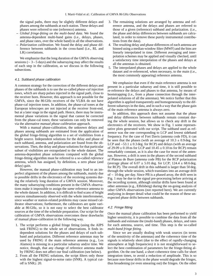
In addition, this approach does not assume that the phaseand delay differences between subbands remain constant dur-ing the whole session, but allows us to check any drift in theelectronics of the receivers. We show in Fig. 1 some represen-tative plots generated with our script. The subband used as ref-erence was the one corresponding to LCP and lowest sidebandfrequency. For the case of Fort Davis (antenna code FD), it canbe seen that the phases (with an average of 10.3 ± 0.9 deg. forLCP and−53.1± 0.3 deg. for RCP) and delays (with an averageof 29.09± 0.18 ns for LCP and 10.45± 0.10 ns for RCP) remainremarkably constant, as it is also the case for most of the anten-nas. However, a drift is seen in the phases of the second subbandof Plateau de Bure (antenna code PB) for the RCP polarization(average phase of 6.07± 5.01 deg. for LCP; 124.4 ± 68.6 deg.for RCP). The overall drift in this subband is larger than 50 deg.through the whole session, which translates into an averagedriftof ∼ 10 deg. per day. Since PB is a phased array, the drift seen inFig. 1 may be due to the signal pre-processing before arriving atthe recording system, although similar drifts have been found atother antennas (e.g., Effelsberg) during the on-going analysis ofother GMVA observations (not reported here). We are currentlyanalyzing in deeper detail what could be the reason of these un-expected phase drifts between subbands.

4.2. Fringe fitting

Once the manual phase calibration has been performed to yieldhigher sensitivity, it is possible to combine the data from all thesubbands and estimate the (multi-band) phases, delays, andratesfor each antenna, source, and time. This step is the so-calledmulti-band fringe fitting.

Since we are usually dealing with weak sources (in termsof the sensitivity of the antennas) and the coherence time ofthesignals is relatively short (due to the effect of rapidly-changingatmosphere at high frequencies) it is not straightforward to se-lect the best combination of parameters for the fringe-fitting al-gorithm. On the one hand, a short coherence time calls for shortintegration times, to avoid a reduction of amplitude. This is sobecause non-linear drifts in the phase would degrade the fringes,thus broadening (or even smearing out) the fringes. On the other

3


0

50

100

150

200

Phase

(deg)

LCPRCP

127 128 129 130 131Time (DOY)

−20

−10

0

10

20

dela

y (

ns)

−50

0

50

Phase

(deg)

LCPRCP

127 128 129 130 131Time (DOY)

0

10

20

30

40

50

dela

y (

ns)

FD subband #2 PB subband #2

Fig. 1.Single-band phases (upper figures) and delays (lower figures) in thesecond subband of Fort Davis (left) and Plateau de Bure (right), referredto Los Alamos, for both circular polarizations. Times are given in day of the year (DOY). The gains are referred to the first subband in the LCPpolarization. Solid lines are the interpolations applied to calibrate the data. Noticethat these plots show data fromall sources.

hand, a short integration time reduces the chance of a successfulfringe detection.

We estimated the best integration time to be used on GMVAdata by analyzing the performance of the global fringe-fittingfor different integration times. For an integration time of 3–4minutes, the number of good (i.e., high SNR) solutions is max-imized with respect to bad, or failed, ones. Since an integrationtime of 3–4 minutes is much longer than the actual (expected)atmosphere coherence time at 86 GHz (i.e,∼ 10− 20 seconds),our results indicate that the changes in the fringe rate due to theatmosphere are not so severe and/or systematic as to break downthe phase coherence during an integration time longer than theexpected∼ 10− 20 seconds, although the exact coherence timewill depend, of course, on the weather conditions at each station(humidity, wind speed, etc.). In other words, the phase fluctua-tions are mostly around an average slope (on a time scale muchlonger than that of the wrapping of the phase, for reasonablygood weather conditions). Hence, if we apply the global fringefitting using long integration times, we will be able to estimateand remove the main slope in the time evolution of the visibilityphases, thus improving the signal coherence (see, e.g., Rogerset al. 1984; Baath et al. 1992; and Rogers, Doeleman, & Moran1995, for additional discussions on the phase coherence in high-frequency VLBI observations). As an example of the quality inthe coherence of the GMVA phases, Fig. 2 shows the fringe-rate spectra at two baselines (Effelsberg to Los Alamos and KittPeak to Los Alamos) for an observation of source 3C 273B, withan integration time of 4 minutes. Notice the sharp peaks in thefringe rates after such a long integration time (and especially forEF-LA, which is one of the longer baselines).

Based on these results, our script for the GMVA calibrationuses a mixed approach, to optimize the performance of the globalfringe fitting. First, a preliminary fringe fitting is executed us-ing a long integration time (4 minutes) and a low SNR cut-off(SNR>4.5). Then, the script reads the estimated antenna delaysand bins them in time using a median window filter. Finally, the

IF 1(LL)

Rate (mHz)-200 -100 0 100 200

6

5

4

3

2

1

0

Fringe rate spectrum (Jy) Baseline: KP - LA

IF 1(LL)

Rate (mHz)-200 -100 0 100 200

600

500

400

300

200

100

0

Fringe rate spectrum (mJy). Baseline: EF - LA

KP − LA

EF − LA

Fig. 2. Fringe-rate spectra at the baselines of Effelsberg to Los Alamos(EF-LA, baseline of 7831 km) and Kitt Peak to Los Alamos (KP-LA,baseline of 752 km), for an observation of source 3C 273B with an in-tegration time of 4 minutes.

4


127 128 129 130 131Time (DOY)

−62

−61

−60

−59

−58

−57

−56

−55

MB

dela

y (

ns)

LCPRCP

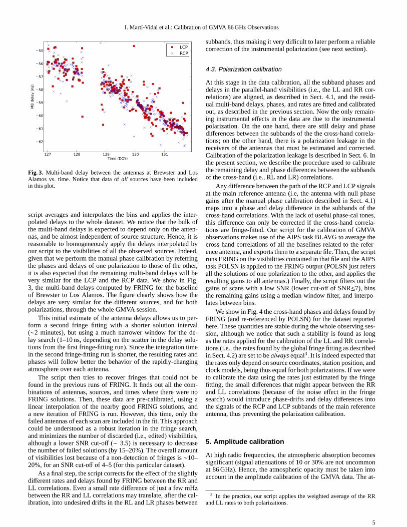
Fig. 3. Multi-band delay between the antennas at Brewster and LosAlamos vs. time. Notice that data ofall sources have been includedin this plot.

script averages and interpolates the bins and applies the inter-polated delays to the whole dataset. We notice that the bulk ofthe multi-band delays is expected to depend only on the anten-nas, and be almost independent of source structure. Hence, it isreasonable to homogeneously apply the delays interpolatedbyour script to the visibilities of all the observed sources. Indeed,given that we perform the manual phase calibration by referringthe phases and delays of one polarization to those of the other,it is also expected that the remaining multi-band delays will bevery similar for the LCP and the RCP data. We show in Fig.3, the multi-band delays computed by FRING for the baselineof Brewster to Los Alamos. The figure clearly shows how thedelays are very similar for the different sources, and for bothpolarizations, through the whole GMVA session.

This initial estimate of the antenna delays allows us to per-form a second fringe fitting with a shorter solution interval(∼2 minutes), but using a much narrower window for the de-lay search (1–10 ns, depending on the scatter in the delay solu-tions from the first fringe-fitting run). Since the integration timein the second fringe-fitting run is shorter, the resulting rates andphases will follow better the behavior of the rapidly-changingatmosphere over each antenna.

The script then tries to recover fringes that could not befound in the previous runs of FRING. It finds out all the com-binations of antennas, sources, and times where there were noFRING solutions. Then, these data are pre-calibrated, using alinear interpolation of the nearby good FRING solutions, anda new iteration of FRING is run. However, this time, only thefailed antennas of each scan are included in the fit. This approachcould be understood as a robust iteration in the fringe search,and minimizes the number of discarded (i.e., edited) visibilities,although a lower SNR cut-off (∼ 3.5) is necessary to decreasethe number of failed solutions (by 15–20%). The overall amountof visibilities lost because of a non-detection of fringes is∼10–20%, for an SNR cut-off of 4–5 (for this particular dataset).

As a final step, the script corrects for the effect of the slightlydifferent rates and delays found by FRING between the RR andLL correlations. Even a small rate difference of just a few mHzbetween the RR and LL correlations may translate, after the cal-ibration, into undesired drifts in the RL and LR phases between

subbands, thus making it very difficult to later perform a reliablecorrection of the instrumental polarization (see next section).

4.3. Polarization calibration

At this stage in the data calibration, all the subband phasesanddelays in the parallel-hand visibilities (i.e., the LL and RR cor-relations) are aligned, as described in Sect. 4.1, and the resid-ual multi-band delays, phases, and rates are fitted and calibratedout, as described in the previous section. Now the only remain-ing instrumental effects in the data are due to the instrumentalpolarization. On the one hand, there are still delay and phasedifferences between the subbands of the the cross-hand correla-tions; on the other hand, there is a polarization leakage in thereceivers of the antennas that must be estimated and corrected.Calibration of the polarization leakage is described in Sect. 6. Inthe present section, we describe the procedure used to calibratethe remaining delay and phase differences between the subbandsof the cross-hand (i.e., RL and LR) correlations.

Any difference between the path of the RCP and LCP signalsat the main reference antenna (i.e, the antenna with null phasegains after the manual phase calibration described in Sect.4.1)maps into a phase and delay difference in the subbands of thecross-hand correlations. With the lack of useful phase-caltones,this difference can only be corrected if the cross-hand correla-tions are fringe-fitted. Our script for the calibration of GMVAobservations makes use of the AIPS task BLAVG to average thecross-hand correlations of all the baselines related to therefer-ence antenna, and exports them to a separate file. Then, the scriptruns FRING on the visibilities contained in that file and the AIPStask POLSN is applied to the FRING output (POLSN just refersall the solutions of one polarization to the other, and applies theresulting gains to all antennas.) Finally, the script filters out thegains of scans with a low SNR (lower cut-off of SNR≤7), binsthe remaining gains using a median window filter, and interpo-lates between bins.

We show in Fig. 4 the cross-hand phases and delays found byFRING (and re-referenced by POLSN) for the dataset reportedhere. These quantities are stable during the whole observing ses-sion, although we notice that such a stability is found as longas the rates applied for the calibration of the LL and RR correla-tions (i.e., the rates found by the global fringe fitting as describedin Sect. 4.2) are set to bealwaysequal3. It is indeed expected thatthe rates only depend on source coordinates, station position, andclock models, being thus equal for both polarizations. If wewereto calibrate the data using the rates just estimated by the fringefitting, the small differences that might appear between the RRand LL correlations (because of the noise effect in the fringesearch) would introduce phase-drifts and delay differences intothe signals of the RCP and LCP subbands of the main referenceantenna, thus preventing the polarization calibration.

5. Amplitude calibration

At high radio frequencies, the atmospheric absorption becomessignificant (signal attenuations of 10 or 30% are not uncommonat 86 GHz). Hence, the atmospheric opacity must be taken intoaccount in the amplitude calibration of the GMVA data. The at-

3 In the practice, our script applies the weighted average of the RRand LL rates to both polarizations.

5


127 128 129 130 131Time (DOY)

0

5

10

15

20

Delay (ns.)

IF 1IF 2

IF 3IF 4

127 128 129 130 131Time (DOY)

0

50

100

Phase (deg.)

IF 1IF 2

IF 3IF 4

Fig. 4.Left, delay differences between LCP and RCP at Los Alamos. Right, phase differences at the same station (referred to those in the subbandat the lowest frequency, IF1).

mospheric opacityτ is estimated at each station (and for eachtime) using the well-known formula

τ = log

(

1−Tsys− Trec

Tamb

)

, (1)

whereTsys is the (opacity-uncorrected) system temperature andTrec is the temperature of the receiver. In this equation, it is as-sumed that the sky temperature (i.e.,Tsys− Trec) is equal to theaverage temperature of the atmosphere (Tamb) corrected by theabsorption factor exp (τ). The spill-over correction and the an-tenna temperature due to the source are very small quantities(less than a few K), so that they can be neglected. If a noisediode is used for the signal calibration,Tsys is directly measuredat the backend of each antenna receiver and for each scan;Tambcan be estimated from the weather monitoring at each station.If the calibration strategy is based on a chopper wheel, the sys-tem directly measures the opacity-corrected system temperature(i.e., Tsysexp (τ)). In regard toTrec, it is assumed to be a stablequantity at a time scale of one day or more.

We estimate the receiver temperature for each station (andpolarization) by fitting the lower envelope of theTsys vs. airmassdistribution with a linear model. Then, the extrapolation of thatmodel to a null airmass gives us a good estimate of the receivertemperature in the time range considered. We show in Fig. 5(left) a sample plot ofTsys vs. airmass, together with the fit tothe lower envelope, for the Los Alamos station. It can be seenin the figure that the receiver temperature is slightly different foreach polarization. However, we notice that our script forces theslopes of the lower envelopes to be the same at both polarizations(since the contribution of the atmosphere toTsys is independentof the polarization). We show in Fig. 5 (right) the resultingtimeevolution of the opacity at zenith (i.e., corrected by the sine ofthe elevation) at Los Alamos. Once the opacity is known, thecorrected system temperature,T∗, is easily computed as

T∗sys= Tsysexp (τ). (2)

There may be cases where an opacity correction has beenalready applied to theTsys values provided by a given station(e.g., Plateau de Bure, Pico Veleta, or Onsala). In those cases,

a differential (or refined) opacity correction can still be appliedusing the approach described here4. There is also the possibilityof applying a constant (zenith-)opacity correction to those an-tennae where it is not possible to find precise estimates of thereceiver temperature. In any case, our goal in the processing ofeach GMVA dataset is to provide the end user with a calibrationtable including all the opacity-corrected gains, as well asa set ofAIPS-friendly files with all theT∗sys estimates (i.e., the opacity-corrected temperatures) and the originalTsys values measured ateach station (in case that the user would like to apply a differentapproach to correct for the atmospheric opacity).

6. Polarization leakage

The LCP and RCP signals from the sources are separated in thefrontend of the receivers, and follow different paths in the elec-tronics. However, the receivers are not perfect, and there is acertain level ofcross-talkbetween the RCP and LCP signals.Hence, the RCP (LCP) signal recorded at each station is in-deed equal to the true RCP (LCP) signal from the source, plusan unknown fraction of LCP (RCP) signal modified by a phasegain. The (complex) factors that account for the fraction ofLCP(RCP) source signal transferred to the recorded RCP (LCP) sig-nals are the so-calledD-terms, and may be different at each an-tenna and for each polarization (for a deep discussion on thepo-larization leakage and its correction with theD-term approach,see Leppanen et al. 1995). The antenna D-terms are expectedto depend only on the station hardware, and be stable quanti-ties over periods of the order of one year (Gomez et al. 2002),although this may depend on the observing frequency. In thissection, we describe how the D-terms are estimated, and howare their effects corrected in the GMVA observations.

Once the data are calibrated in both phase and amplitude,we perform a deep hybrid imaging with the program Difmap(Shepherd et al. 1994), by applying phase and amplitude self-calibration under reasonable limits, and taking special care withnoisier data (since, in those cases, there may be a large probabil-

4 At IRAM opacities are obtained using an atmospheric model, so arenot free from assumptions.

6


1 2 3 4 5Airmass

140

160

180

200

220

240

260Tsys (K)

LCPRCP

127 128 129 130 131Time (DOY)

0.08

0.09

0.10

0.11

0.12

0.13

Zenith Opacity (np)

Fig. 5. Left, system temperatures (Tsys) measured at Los Alamos vs. airmass. Straight lines are fits of linear models to the lower envelopes of theTsys distributions. The receiver temperature is estimated as the extrapolation ofthe lower envelope to a null airmass. Right, zenith opacity (i.e.,opacity multiplied by the sine of the antenna elevation) at Los Alamos vs. time, as estimated using Eq. 1.

ity of generating spurious components in the source structures;e.g., Martı-Vidal & Marcaide 2008). To ensure optimum resultsall the hybrid imaging is performed without scripting.

The final images and calibrated data are then read back intoAIPS by the script, source by source. The AIPS task CALIB isexecuted to perform the correction of any possible RCP-to-LCPamplitude bias at the antennas (by assuming a zero circular po-larization for all the sources). The CLEAN components corre-sponding to the main features in the structure of each sourcearethen joined with the AIPS task CCEDT (the regions defining themain features in the source structures have already been selectedmanually, after the hybrid imaging). Finally, the task LPCAL es-timates the D-terms of each antenna, as well as the polarizationof the different source components.

We notice that the accuracy of the D-term determinationdepends on the strength of the detected cross-polarized signal,which may be higher if the source is strongly polarized or ifthe antenna has strong intrinsic cross-polarization (but it shouldbe below of 10%, to avoid problems with the linear approxima-tion used in LPCAL). The accuracy also depends on the uni-formity and range of the parallactic angle coverage and, to alesser extend, also on the complexity of the polarized source sub-structure.

6.1. D-terms and image fidelity

Since the D-terms are estimated using the data of each sourceseparately, we have as many estimates of antenna D-terms assources (we are currently working on the possibility of fittingone single set of D-terms to the visibilities of all sources,simul-taneously, which would result in a more robust modeling of thepolarization leakage). The final D-terms that we apply to eachantenna are a weighted average of all estimated D-terms. Priorto the average, any clear outliers are removed, and the relativeweights are adjusted as a function of the source flux density(and its fraction of polarized emission); the higher the signal ofthe source in the cross-hand correlations, the higher the weightof the corresponding D-terms in the average. This approach isvery similar to those reported in previous publications discussinghigh-frequency VLBI polarimetry (e.g. Marscher et al. 2002).

We give the average D-term amplitudes of all the antennas inTable 1 (Col. 6). We notice that the dispersion in the D-termses-

timated from the visibilities of the different sources is large (seethe uncertainties in the amplitude averages!). Such a largedis-persion in the D-term estimates is indicative of a strong coupling(in the LPCAL fitting) between the polarization leakage and thepolarized source components, which maps into a poor modelingof the polarization leakage. We also notice that the visibilitiesin the cross-hand correlations are quite sensitive to the leakage,so the final full-polarization GMVA images may differ notably,depending on the different schemes used for the estimate of theD-terms.

However, it would be expected that the main polarizationfeatures in the images (i.e., the source components with thestrongest polarized emission) are rather insensitive to changesin the estimated D-terms. Moreover, there may also be corre-lations in the D-terms (i.e., couplings in the D-term estimatesat the different antennas, resulting from the fitting procedure inLPCAL), such that images obtained from the use of differentsets of D-terms do not differ significantly. We performed a quan-titative analysis of how strongly the GMVA polarization imagesdiffer as a function of the different weighting schemes in theD-term averaging. In our analysis, we have estimated the high-est dynamic range achievable in the polarization images, suchthat the result should be nearly independent of the weights ap-plied in the D-term averaging. This analysis is based on a MonteCarlo approach, and is described in the following lines. Foreachsource:

1. We generate the dirty image of the Stokes parameters Q andU, calibrated using the vector-averaged D-terms (which areobtained as described in Sect. 6). Let us call this result thereference polarization image.

2. We compute a new vector-average of the D-terms, but usingrandom weights for the different sources (weights uniformlydistributed between 0 and 1).

3. We generate the dirty images of the Stokes parameters Q andU using these new D-terms, and subtract these images fromthe reference image (i.e., that generated in step 1). Let us callthese resultsdifferential polarization images.

4. We compute the ratio between the intensity peaks in the dif-ferential images (i.e., those generated in step 3) and the in-tensity peak in the reference image (i.e., that generated instep 1).

7


0.0 0.2 0.4 0.6 0.8 1.0Peak ratio (diff. image / pol. image)

0

20

40

60

80

100

120

140

160

180

# of D-term

calib

rations.

Fig. 6.Distribution of the intensity peaks of thedifferential polarizationimages(see text) of source 3C 345, divided the peak of the referencepolarization image.

5. We iterate steps 2 to 4.

The intensity peaks in the differential images (i.e., those instep 3) give us an estimate of how different are the images whenwe (randomly) change the weights of the D-terms in the average.Ideally, the peaks in these images should be zero (i.e., the imagesgenerated in step 1 and step 3 should be equal), regardless oftheweighting scheme used to compute the average of the D-terms.Hence, the ratio between the intensity peak in the differential im-ages and the peak of the (D-term corrected) polarization imagewill be a measure of the dynamic range achievable, such thatthe images are independent of the different weights applied tothe D-terms. In other words, the peaks in the differential imagesare lower bounds to the flux density per unit beam of the sourcecomponents that are almost insensitive to changes in the D-termsaveraging.

In Fig. 6, we show the distribution of intensity peaks in thedifferential polarization images of source 3C 345, using a totalof 1000 Monte Carlo iterations. The cut-off probability of 95%(i.e., 2 sigma) for the null hypothesis of a false detection corre-sponds to a peak intensity of∼0.65 times the peak in the polar-ization image. Hence, any source component with a flux densitylarger than∼0.65 times that of the peak can be considered asreal, with a confidence of 95%.

The images obtained using different D-terms do not only dif-fer in the strength of the polarized features, but also in their lo-cation. Indeed, many of the Monte Carlo iterations where wefound large peaks in the differential images correspond to caseswhere the peaks of the Monte Carlo images were slightly shiftedwith respect to the peak of the reference polarization image. Weshow in Fig. 7(a) the distribution of shifts between the peakofthe reference image and the peak of the images obtained fromall the Monte Carlo iterations. Most of the Monte Carlo imageshave their peaks at less than 30µas away from the peak of ourreference polarization image (this is roughly the size of the mi-nor axis of our beam). If we take into account these small shiftsin the computation of the differential polarization images, the re-sulting peaks of the new differential images are quite lower thanthose without shifting, as we show in Fig. 7(b). Hence, if thesmall shifts are corrected, the final images do not typicallydif-fer at a level of more than 50–60% of the source peak (with aconfidence interval of 95%). The position shifts obtained from

0.0 0.2 0.4 0.6 0.8 1.0Peak ratio (shifted diff. image / pol. image)

0

50

100

150

200

250

300

350

# o

f D-term

calib

rations.

0.00 0.01 0.02 0.03 0.04 0.05 0.06 0.07 0.08 0.09Peak shift (mas)

0

50

100

150

200

250

300

350

400

450

# o

f D-term

calib

rations.

(b)

(a)

Fig. 7.(a) Distribution of the shifts in the intensity peaks of all the polar-ization images obtained in our Monte Carlo D-terms analysis. (b) Sameas Fig. 6, but taking into account the peak shifts before computing thedifferential polarization images.

the different D-term calibration also imply that the astrometricprecision in the location of the polarized emission is of theorderof ∼30µas (roughly the size of the minor axis of the synthesizedbeam).

7. Representative images

Once the data are calibrated as described in the previous sec-tions, they are ready for a full-polarization imaging (taking intoaccount the polarization limitations described in Sect. 6.1). Wepresent, in Fig. 8, a sample image of the source 3C 345 obtainedfrom the GMVA observations reported here. The high qualityof the GMVA data allows us to recover extended jet structuredistant from the core, after careful imaging, including iterativeamplitude self-calibration and uv-tapering. We also show in Fig.9 two polarization images of the same source, obtained fromdifferent estimates of the antenna D-terms (i.e., averaging theD-terms estimated from the visibilities of a selection of sourcesor using the D-terms just estimated from the visibilities 3C345).The polarization is very similar in both images (we applied acut-off at 60% of the polarization peak). There is polarized emissionat the north-east side of the core, where the electric-vector posi-tion angle (EVPA) is perpendicular to the jet. Then, the electric

8


Center at RA = 16h 42m 58.80996672s Dec = 39d 48’ 36.9939808"

Cont peak flux = 1.11 Jy/beam Levs = (-0.5, 0.5, 1, 2, 4, 8, 16, 32, 64, 90)% of peak

0.0 0.5 1.0R

elat

ive

Dec

(m

as)

Relative RA (mas)0.0 -0.2 -0.4 -0.6 -0.8

0.3

0.2

0.1

0.0

-0.1

-0.2

-0.3


Cont peak flux = 3.45 Jy/beam Levs = (-0.5, 0.5, 1, 2, 4, 8, 16, 32, 64, 90)% of peak

0 1 2 3

Rel

ativ

e D

ec (

mas

)

Relative RA (mas)0 -1 -2 -3 -4 -5

1.0

0.5

0.0

-0.5

-1.0

(a)

(b)

Fig. 8. Total-intensity images of 3C 345 obtained from the analysis ofthe GMVA data taken on May 2010. The full width at half maximum(FWHM) of the restoring beams are shown at the bottom-left corners.(a) using uniform weighting of the visibilities (restoring beam withFWHM of 110×38µas with a position angle of−4.37 deg.). (b) usingnatural weighting of the visibilities and tapering longest baselines (toenhance the sensitivity to extended structures; FWHM of 270×230µaswith a position angle of 62 deg.).

vector position angle rotates as the distance to the core increaseswestwards. The polarization images in Fig. 9 can be comparedto another image obtained from VLBI observations at 43 GHz(Jorstad et al., in prep.) taken on 19 May 2010, only a few daysbefore our GMVA session. We show the 43 GHz image (onlythe part near the VLBI core of the source) in Fig. 10. The elec-tric vector position angle at 43 GHz is very similar to that ofthe optically-thin components in Fig. 9 (i.e., the western compo-nents, away from the core at 86 GHz), although we notice thatthe absolute electric-vector position angle (i.e., a possible globalR-L phase offset at the reference antenna, which would map intoa global rotation of all the polarization vectors in the image) hasnot been determined in our observations. We also notice thatthepolarized core component with north-south electric vectorposi-tion angle at 86 GHz is not detected at 43 GHz. Possible reasonsof this discrepancy in the polarized emission at different frequen-cies could be opacity, Faraday rotation, or blending (due tothelarger beam at 43 GHz). A deep analysis of Figs. 9 and 10 liesbeyond the scope of the objective of this paper, and will be pub-lished elsewhere.

Center at RA = 16h 42m 58.80996672s DEC 39d 48’ 36.9939808"

Cont peak flux = 1.55 Jy/beam

Levs = (-0.5, 0.5, 1, 2, 4, 8, 16,32, 64, 90)% of peakPol. line (1 mas) = 2.5 Jy/beam

Rel

ativ

e D

ec (

mas

)

Relative RA (mas)0.4 0.2 0.0 -0.2 -0.4 -0.6 -0.8

0.4

0.2

0.0

-0.2

-0.4

-0.6

Fig. 10. VLBI image of the inner core region of 3C345 at 43 GHz(Jorstad et al., in prep.), observed on 19 May 2010.

8. Summary

We report a well-defined calibration pipeline for globalmillimeter-VLBI (GMVA) observations. With this pipeline,it ispossible to estimate all the instrumental effects in an optimumway, dealing with the particulars of the (typically complicated)schedules of global 3mm VLBI observations and the inherentcomplications due to the high observing frequency (86 GHz).Allthe scripts used in the pipeline are written in a generic way,sothey can be easily executed and adapted for all the GMVA (andeventually non-GMVA) datasets. Indeed, these scripts willstillbe valid if new stations eventually join the GMVA in a near fu-ture.

The scripts allow us to perform manual phase calibration(i.e., alignment of the phases among the different sub-bands)regardless of the subarraying conditions typically found in thedata. The script also corrects for time dependent phase and delaydrifts between subbands caused by variations in the electronicsof the antenna receivers.

We perform the global fringe fitting (GFF) by optimizing theintegration time of the fringes within the real coherence time ofthe visibilities. In the case of the GMVA, we show that at 86GHz integration times of up to several minutes maximize theSNR of the fringes, indicative of an only moderate atmosphericdegradation of the incoming phase.

The visibility amplitudes are calibrated by fitting the temper-ature of the receivers of each antenna (and polarization) tothedistribution of system temperatures over airmass. The opacity isthen directly derived from the ambient and system temperaturesfor each antenna and time. For the cases of antennas where theatmospheric absorption is directly accounted in the amplitudecalibration, we can still refine the opacity correction withourapproach.

For the polarization calibration, we perform manual phasecalibration on the cross-polarization visibilities (i.e., we alignthe phases of the cross-polarization visibilities among the sub-bands) by imposing the same fringe rates in both polarizationsfor all the antennas and times. This calibration allows us tode-termine the leakage in the receivers (i.e., the D-terms) using thedata of all sub-bands together, thus duplicating the SNR withrespect to the D-terms estimated from independent fits to thedifferent subbands.

Our scripts also allow us to perform a Monte Carlo analysisto determine the effect of different D-term calibrations on the fi-nal full-polarization images. For the data reported here, acut-offin the polarization images at a level of 50–60% of the intensitypeak generates images that are typically very similar, regardless

9


Pol. line (1 mas) = 4.5 Jy/beam

Rel

ativ

e D

ec (

mas

)

Relative RA (mas)0.05 0 -0.05 -0.1 -0.15 -0.2 -0.25

0.2

0.1

0

-0.1

-0.2


Cont peak flux = 1.11 Jy/beam

Levs = (-0.5, 0.5, 1, 2, 4, 8, 16, 32, 64, 90)% of peakPol. line (1 mas) = 4.5 Jy/beam

Rel

ativ

e D

ec (

mas

)

Relative RA (mas)0.05 0 -0.05 -0.1 -0.15 -0.2 -0.25

0.2

0.1

0

-0.1

-0.2

(b)(a)

Fig. 9. Polarization images (superimposed to the total-intensity image) of 3C 345. The FWHM of the restoring beam is shown at the bottom-leftcorners. (a) averaging the D-terms estimated from the visibilities of 3C 345, BLLAC, and 0716+714. (b) using the D-terms directly estimated fromthe visibilities of 3C 345.

of the D-term calibration. The absolute position of the polariza-tion features can also be affected by the D-term calibration, butthis effect is not larger than the size of the the synthesized beam.

As an example of our pipeline output, we show full-polarization images of source 3C 345, obtained from observa-tions performed during the GMVA session of May 2010. Thepolarization images show a strong component at the northeastside of the source core, with a north-south electric vector posi-tion angle that rotates counter-clockwise along the jet (i.e., alongthe west direction). There are also two polarization componentsat about 0.1 and 0.2 mas from the core, with an electric vectorpo-sition angle aligned to the direction of the jet and similar to theelectric vector position angle observed at 43 GHz from VLBAobservations taken a few days before our GMVA session.

In forthcoming GMVA sessions, we expect to be able to pro-vide the end user with fully calibrated datasets, obtained shortafter the data correlation.

Acknowledgements.The National Radio Astronomy Observatory is a facilityof the National Science Foundation operated under cooperative agreement byAssociated Universities, Inc. Based on observations with the 100-m telescope ofthe MPIfR (Max-Planck-Institut fur Radioastronomie) at Effelsberg. Based onobservations carried out with the IRAM Plateau de Bure Interferometer and theIRAM telescope at Pico Veleta. IRAM is supported by INSU/CNRS (France),MPG (Germany) and IGN (Spain).

References

Attridge J.M. 2001, ApJ, 553, L31Attridge J.M., Wardle J.F.C., Homan D.C., & Phillips R.B. 2005, ASPC, 340,

171Baath L.B., Rogers A.E.E., Inoue M., et al. 1992, A&A, 257, 31Broderick A.E. & Loeb A. 2009, ApJ, 697, 1164Dodson R. 2009, arXiv:0910.1707DGomez J.L., Marscher A.P., Alberdi A., et al. 2002, VLBA Scientific Memo #30Gomez J.L., Roca-Sogorb M., Agudo I., et al. 2011, ApJ, 733, 11Homan D.C., Lister M.L., Aller H.D., et al. 2009, ApJ, 696, 328Kettenis M., van Langevelde H.J., Reynolds C., & Cotton B. 2006, ASPC, 351,

497Leppannen K.J., Zensus A.J. & Diamond P.J. 1995, AJ, 110, 2479Marscher A.P., Svetlana G.J., John P.M., et al. 2002, ApJ, 577, 85Martı-Vidal I. & Marcaide J.M. 2008, A&A, 480, 289Mc Kinney J.C., Tchekhovskoy A., & Blandford R.D. 2012, arXiv:1201.4163O’ Sullivan S.P., Gabuzda D.C., Gurvits L.I. 2011, MNRAS, 415, 3049

Penzias A.A., Burrus C.A. 1973, ARA&A, 11, 51Rogers A.E.E., Moffet A.T., Backer D.C., & Moran J.M. 1984, Radio Science,

19, 1552Rogers A.E.E., Doeleman S.S., & Moran J.M. 1995, AJ, 109, 1391Shepherd M.C., Pearson T.J., & Taylor G.B. 1994, BAAS, 26, 987Schwab F.R. & Cotton W.D. 1983, AJ, 88, 688Tchekhovskoy A., Narayan R., & Mc Kinney J.C. 2011, MNRAS, 418, L79

10

on the calibration of full-polarization 86ghz global...

Documents