on the calculation of full and partial directivity indices · in this document, the partial...

3D Audio and Applied Acoustics Laboratory · Princeton University

On the Calculation of Full and Partial Directivity Indices

Joseph G. Tylka Edgar Y. [email protected] [email protected]

Revised version – February 19th, 2016Original version – November 16th, 2014

Abstract

A set of metrics is presented which quantifies, using measured power spectra, the directivityof a loudspeaker, relative either to the full sphere or to a given hemisphere, plane, or half-plane.The former, called the directivity index (DI), is a commonly-used metric, but is only definedfor complete sets of measurements. The latter metrics, called partial directivity indices, extendthe definition of the DI to isolate sections of the loudspeaker’s radiation pattern (e.g., forwardradiation alone) and quantify its directivity over those sections. In general, all DI spectra aregiven by the ratio between the on-axis power spectrum and a weighted average of a certain subsetof power spectra. For the spherical and hemispherical cases, each weight is proportional to thesurface area of the portion of the unit sphere represented by the corresponding measurement,whereas for the planar cases, each weight is proportional to the arc length of the correspondingportion of the unit circle. In this document, the partial directivity indices are defined and therelevant formulae needed to compute them are provided.

1 Introduction

It is a well-known property of modern loudspeakers that sound is not radiated equally in all direc-tions for all frequencies. The directivity of a loudspeaker describes the extent to which the acousticpower produced by the loudspeaker is biased toward a given direction. To quantify directivity, thedirectivity factor (or directivity index when expressed in dB) is defined as the acoustic intensity ata given point on the surface of an imaginary sphere surrounding the loudspeaker relative to theaverage intensity over the entire surface [1, 2]. The directivity factor (index) spectrum is typicallydefined as (ten times the base-ten logarithm of) the ratio between the on-axis power spectrumand the average power spectrum,1 which is approximately computed by averaging measured powerspectra over many directions [2]. In practice, rather than measuring power spectra uniformly dis-tributed on the sphere (a time-consuming and complicated process), measurements are typicallyperformed only along horizontal and vertical “orbits” around the loudspeaker [2]. We shall refer tothe DI spectrum computed with these measurements as the approximate full-sphere DI spectrum.

In this document, we first recall the definitions of the exact and approximate full-sphere DIspectra. We then extend the latter to define three partial DI spectra:

• single plane (horizontal or vertical),

• single hemisphere (frontal or rear), and

• single half-plane (frontal or rear, and horizontal or vertical).

1This average power spectrum over many directions is sometimes called the sound power spectrum [2].

1

mailto:[email protected]

mailto:[email protected]


These partial DI spectra allow certain sections of the radiation pattern to be isolated when evalu-ating directivity. Of particular significance to these definitions are the weighted averages of mea-surements which yield the corresponding average power spectra. Consequently, we discuss thecalculation of appropriate weights based on the geometrical arrangement of the measurements. Wealso discuss the calculation of the average and standard deviation of a given DI spectrum to serveas compact metrics by which to compare the directivities of different loudspeakers. This documentis presented as part of the ongoing experimental survey of loudspeaker directivity at the 3D Audioand Applied Acoustics (3D3A) Laboratory at Princeton University.2

1.1 Coordinate System

In this document, we adopt a spherical coordinate system in accordance with the Audio EngineeringSociety (AES) standard AES56-2008 [3]. A diagram of this coordinate system is shown in Fig. 1.Typically, we define the origin of the coordinate system as the center of the loudspeaker cabinet, anda reference axis which passes through the center of the (upright) loudspeaker cabinet horizontally,parallel to the ground and perpendicular to a specified radiating surface (e.g., the dome of the high-frequency transducer). However, the precise alignment of the loudspeaker in the coordinate systemmay vary for different loudspeakers. We also define a measurement axis which passes through theorigin and the measurement point (i.e., the position of the microphone). The plane defined by thereference axis and the measurement axis is called the measurement plane.

Let θ ∈ [0, π] denote the angle between the measurement axis and the reference axis on themeasurement plane. Also let φ ∈ [0, 2π) denote the angle of the measurement plane about thereference axis, such that φ = 0 when the measurement point is to the left of the loudspeaker(when viewed from the rear) and the measurement plane is parallel to the ground. When viewingthe loudspeaker from the rear, φ increases as the measurement plane rotates clockwise about thereference axis. By this convention, measurements taken along the horizontal orbit will have φ valuesof either 0 (to the left of the loudspeaker) or π (to the right), and those along the vertical orbitwill have φ values of either π/2 (above) or 3π/2 (below). We will also refer to the correspondingCartesian coordinate system, for which the x-axis points in the direction (π/2, 0), the y-axis pointsin the direction (π/2, π/2), and the z-axis points in the direction (0, 0).

2 The Directivity Index

For measurements performed at a fixed distance away from the loudspeaker, let H(ω, θ, φ) denotethe frequency response of the loudspeaker, where ω is angular frequency in rad/sec. We referto the frequency response measured at θ = φ = 0 as the “on-axis” response, and denote it byH0,0 (ω) = H (ω, 0, 0). The directivity index spectrum (in dB) is then given by

DI(ω) = 10 log10

|H0,0 (ω)|2

1

4π

∫ 2π

φ=0

∫ π

θ=0|H (ω, θ, φ)|2 sin θdθdφ

. (1)

2http://www.princeton.edu/3D3A/Directivity.html

2

http://www.princeton.edu/3D3A/Directivity.html


Figure 1: Diagram of the coordinate system. The reference axis (θ = 0) passes through the center ofthe (upright) loudspeaker cabinet, parallel to the ground. The two circles represent the horizontaland vertical measurement orbits.

As it is impossible to measure H for all directions (θ, φ), we must turn to an approximate definitionof the DI spectrum.

Consider a set of 2N directions (θm,n, φm,n) for m = 0, 1 and integer values of n ∈ [0, N − 1],where the value of m indicates the orbit and N is the number of measurements taken along each or-bit. We denote frequency responses measured for these directions by Hm,n (ω) = H (ω, θm,n, φm,n).Let ∆θ = 2π/N denote the angular spacing between measurements in each orbit, and ∆φ = π/2denote the angular spacing between orbits. The full set of measurement directions are then givenby

(θm,n, φm,n) =

(n∆θ,m∆φ) for 0 ≤ n < N

2 ,(π −

(n− N

2

)∆θ, π +m∆φ

)for N

2 ≤ n < N,(2)

where N is an integer multiple of 4 (i.e., the same number of measurements are taken in eachquadrant of each orbit). By this definition, m = 0 corresponds to the horizontal orbit and m = 1corresponds to the vertical orbit. Note that each orbit contains a measurement for the frontalon-axis (θ = 0) response as well as the rear axis (θ = π) response. For measurements taken in the3D3A Lab, we maintain an angular spacing of ∆θ = 5, yielding N = 72 total measurements oneach orbit. A diagram illustrating an example of these measurement directions with an angularspacing of ∆θ = 10 (for clarity) is shown in Fig. 4 (in the appendix).

Given frequency response measurements for each of the directions defined in Eq. (2), the ap-

3


proximate full-sphere DI spectrum (in dB) is given by

DI(ω) = 10 log10

|H0,0 (ω)|21∑

m=0

N−1∑n=0

wn |Hm,n (ω)|2, (3)

where wn is a direction-dependent weight attributed to each measurement. Note that these weightsare normalized such that

1∑m=0

N−1∑n=0

wn = 1.

This formula has been adapted from the method proposed by Davis [4], and later refined by Davis[5, 6] and Wilson [7, 8], in which measurements are equally spaced around each orbit, but weightedaccording to the surface area of the portion of the unit sphere represented by each measurement.This method will be discussed further in Section 4.

3 Partial Directivity Indices

In this section, we define the three types of partial directivity indices listed in Section 1.

3.1 Single Plane

The single plane DI uses measurements performed along a single orbit (either horizontal or vertical)to quantify the ratio between the on-axis acoustic output of the loudspeaker and its total acousticoutput into the measurement plane. As defined by Eq. (2), these directions correspond to n ∈[0, N − 1] and either m = 0 (horizontal) or m = 1 (vertical). A diagram illustrating an example ofthese measurement directions (in the horizontal plane) is shown in Fig. 5.

Given frequency response measurements for these directions, the approximate single-plane DIspectrum (in dB) is given by

DIm(ω) = 10 log10

|Hm,0 (ω)|2

1

N

N−1∑n=0

|Hm,n (ω)|2. (4)

Note that, by this definition, each measurement is given equal weight in the calculation of theaverage power spectrum. This is done because the measurements are equally spaced along themeasurement orbit and, for this particular DI spectrum, we are interested only in the variation ofthe loudspeaker’s frequency response with angle along that orbit.

3.2 Single Hemisphere

The single hemisphere DI uses measurements performed along halves (either frontal or rear) ofboth the horizontal and vertical orbits to quantify the ratio between the on-axis acoustic output

4


of the loudspeaker and its total acoustic output into the measurement half-space (hemisphere). Asdefined by Eq. (2), these directions correspond to m = 0, 1 and either n ∈ [0, N/4] ∪ [3N/4, N − 1](frontal) or n ∈ [N/4, 3N/4] (rear). Due to the inclusion of the end-points, an angular spacingof ∆θ = 5 yields N + 2 = 74 total measurements. A diagram illustrating an example of thesemeasurement directions is shown in Fig. 6.

Given frequency response measurements for these directions, the approximate single-hemisphereDI spectrum (in dB) is given by

DI(ω) = 10 log10

|H0,0 (ω)|21∑

m=0

N−1∑n=0

vn |Hm,n (ω)|2, (5)

where the weights vn in the above equation are related to those used in the definition of thefull-sphere DI spectrum (see Eq. (3)) by, in the case of the frontal hemisphere,

vn =

2wn for n ∈ [0, N/4) ∪ (3N/4, N − 1],

wn for n = N/4, 3N/4,

0 for n ∈ (N/4, 3N/4).

(6)

In the case of the rear hemisphere, the weight values for the first and third cases in Eq. (6) areswapped. Due to the symmetry of the wn weights (as will be seen in Section 4), the vn weights arealso normalized such that

1∑m=0

N−1∑n=0

vn = 1.

Note that the weights at the end-points of each half-orbit (i.e., the four measurements for whichθ = π/2) are reduced by a factor of 2 relative to the other non-zero weights. This is necessarysince the total weight attributed to those measurements in the calculation of the full-sphere DIspectrum (Eq. (3)) represents a portion of the sphere whose surface area is evenly split in front ofand behind the loudspeaker, i.e., between θ = π/2±∆θ/2. Consequently, to compute the averagepower spectrum for the frontal hemisphere only, for example, we include only the forward-radiatingpower by splitting the surface area (and therefore the weight) in half.

3.3 Single Half-Plane

The single half-plane DI uses measurements performed along half (either frontal or rear) of a singleorbit (either horizontal or vertical) to quantify the ratio between the on-axis acoustic output ofthe loudspeaker and its total acoustic output into the measurement half-plane. As defined byEq. (2), these directions correspond to any combination of m = 0 (horizontal) or m = 1 (vertical)and n ∈ [0, N/4] ∪ [3N/4, N − 1] (frontal) or n ∈ [N/4, 3N/4] (rear). Due to the inclusion of theend-points, an angular spacing of ∆θ = 5 yields N/2 + 1 = 37 total measurements. A diagramillustrating an example of these measurement directions is shown in Fig. 7.

5


Given frequency response measurements for these directions, the approximate single-half-planeDI spectrum (in dB) is given by

DIm(ω) = 10 log10

|H0,0 (ω)|2

1

N/2

N−1∑n=0

un |Hm,n (ω)|2, (7)

where the weights un in the above equation are given by, in the case of a frontal half-plane,

un =

1 for n ∈ [0, N/4) ∪ (3N/4, N − 1],12 for n = N/4, 3N/4,

0 for n ∈ (N/4, 3N/4).

(8)

In the case of a rear half-plane, the weight values for the first and third cases in Eq. (8) are swapped.It is easily shown that these weights satisfy

N−1∑n=0

un = N/2.

Note that, as in the single-plane DI spectrum definition given in Eq. (4), all measurements, withthe exception of those at the end-points, are given equal weight in the calculation of the averagepower spectrum. However, as in the single-hemisphere DI spectrum definition given in Eqs. (5)and (6), the weights of the end-point measurements are reduced by a factor of 2.

4 Weight Calculations

As mentioned above, in order to compute the full-sphere and single-hemisphere DI spectra, we mustcompute a weighted average of frequency response measurements. In this section, we describe howthe appropriate weights are calculated. This method follows the same formulation as that proposedby Wilson [7, 8], which itself is equivalent to the graphical method proposed by Kendig and Mueser[9].

Consider a plane perpendicular to the z-axis at some distance z ∈ [−1, 1] from the origin. Theintersection of this plane and the unit sphere defines a circle (or a point if |z| = 1) consisting of alldirections which satisfy z = cos θ. The surface area of the portion of the unit sphere (i.e., the solidangle) for which z ≥ cos θ is given by

Ω(θ) =

∫ 2π

φ=0

∫ θ

θ′=0sin θ′dθ′dφ = 2π(1− cos θ), (9)

where θ′ is a variable of integration and Ω is given in sr.We use the above equation to compute weights that correspond to the surface area of the unit

sphere represented by each measurement. For example, the surface area represented by an on-axismeasurement (for which θ = 0) is given by Ω(∆θ/2). This surface can be visualized as a “spherical

6


(a) w0 (b) w1 (c) w2

Figure 2: Surface areas corresponding to various weight calculations.

cap,” as illustrated in Fig. 2a. In the case of measurements along both the horizontal and verticalorbits, the total surface area of the unit sphere represented by the four measurements of the sameθ is given by Ω(θ+ ∆θ/2)−Ω(θ−∆θ/2). Such a surface can be visualized as a “strip” around thesphere, as illustrated in Figs. 2b and 2c.

Following the numbering convention defined by Eq. (2), the first few weights for the calculationof the average power spectrum are given by

w0 =1

4π

Ω(

∆θ2

)2

, (10)

w1 =1

4π

Ω(∆θ + ∆θ

2

)− Ω

(∆θ − ∆θ

2

)4

, and (11)

w2 =1

4π

Ω(2∆θ + ∆θ

2

)− Ω

(2∆θ − ∆θ

2

)4

. (12)

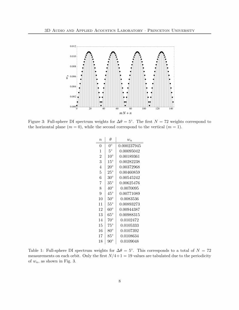
In the above equations, the on-axis weight w0 is divided by 2 since the surface area of the sphericalcap must be evenly split between the on-axis measurement from the horizontal orbit and that fromthe vertical orbit. Similarly, both the weights w1 and w2 are divided by 4 since the surface area ofthe strip around the sphere must be evenly split between the two measurements from the horizontalorbit and those from the vertical orbit. The remaining weights for a given set of measurementsmay be calculated by extending the pattern established by the above equations. Figure 3 shows thefull set of weights for the calculation of the approximate full-sphere DI spectrum with an angularspacing between measurements of ∆θ = 5. A certain subset of these weights is applied in thecalculation of the approximate single-hemisphere DI spectrum, as given by Eq. (6).

It is useful to note that the full set of weights will exhibit a certain periodicity, as seen in Fig. 3,due to the symmetry of the measurements along each orbit. Indeed, only the first N/4 + 1 weightsfor the calculation of the approximate full-sphere DI spectrum need to be computed explicitly.These values are tabulated in Table 1 for an angular spacing of ∆θ = 5.

7


+

Figure 3: Full-sphere DI spectrum weights for ∆θ = 5. The first N = 72 weights correspond tothe horizontal plane (m = 0), while the second correspond to the vertical (m = 1).

n θ wn

0 0 0.0002379451 5 0.000950422 10 0.001893613 15 0.002822384 20 0.003729685 25 0.004608596 30 0.005452427 35 0.006254768 40 0.00700959 45 0.0077108910 50 0.008353611 55 0.0089327312 60 0.0094438713 65 0.0098831514 70 0.010247215 75 0.010533316 80 0.010739217 85 0.010863418 90 0.0109048

Table 1: Full-sphere DI spectrum weights for ∆θ = 5. This corresponds to a total of N = 72measurements on each orbit. Only the first N/4+1 = 19 values are tabulated due to the periodicityof wn, as shown in Fig. 3.

8


5 Average Directivity Index

In order to more easily compare the directivity of different loudspeakers, we now define an averageDI value. This value is computed by averaging the DI spectrum over a certain range of frequencies.For measurements taken in the 3D3A Lab, we compute a logarithmically-weighted average of eachapproximate DI spectrum from 100 Hz to 20 kHz.

In practice, the frequency responses used in the various DI spectra definitions given in previoussections are computed via the fast Fourier transform (FFT). Therefore, the discrete frequenciesover which any frequency spectrum is defined are uniformly spaced between 0 Hz (DC) and thesampling frequency. The frequency index, k ∈ [0,K − 1], is proportional to the actual frequency inHz, given by the relationship

f [k] =Fsk

K, (13)

where K is the number of FFT points and Fs is the sampling frequency.Rather than computing the arithmetic mean of the DI spectrum on a linear frequency scale,

we compute a weighted average which approximates averaging the spectrum over a logarithmicfrequency scale. The average DI spectrum value (in dB) over the range k ∈ [k1, k2] is then given by

DI =

k2∑k=k1

W [k] ·DI[k]

k2∑k=k1

W [k]

, (14)

where k1 < k2 ≤ K/2 and W [k] is a sequence of weights given by

W [k] = logk + 0.5

k − 0.5. (15)

Similarly, the variance of the DI spectrum over the same frequency range is given by

σ2DI =

k2∑k=k1

W [k](DI[k]−DI

)2k2∑

k=k1

W [k]

. (16)

The standard deviation, σDI, may be used to quantify the extent to which the loudspeaker exhibitsconstant directivity, as a small standard deviation indicates that the DI is constant with frequency.This, however, does not guarantee constant directivity, as a small σDI means only that the ratiobetween the on-axis and the average power spectrum remains nearly constant with frequency – thepolar radiation pattern may still vary with frequency. Additional metrics for constant directivitywill be discussed in a future publication.

9


References

[1] C. T. Molloy. Calculation of the Directivity Index for Various Types of Radiators. The Journalof the Acoustical Society of America, 20(4):387–405, July 1943.

[2] Floyd E. Toole. Sound Reproduction: Loudspeakers and Rooms. Focal Press, 2008.

[3] AES56-2008: AES standard on acoustics - Sound source modeling - Loudspeaker polar radiationmeasurements, 2008 (reaffirmed 2014).

[4] Don Davis. A Proposed Standard Method of Measuring the Directivity Factor “Q” of Loud-speakers Used in Commercial Sound Work. J. Audio Eng. Soc., 21(7):571–578, 1973. URLhttp://www.aes.org/e-lib/browse.cfm?elib=1948.

[5] Don Davis. On Standardizing the Measurement of Q. J. Audio Eng. Soc. (Forum), 21(9):730–731, 1973.

[6] Don Davis. Further Comments on Directivity Factor. J. Audio Eng. Soc. (Forum), 21(10):827–828, 1973. URL http://www.aes.org/e-lib/browse.cfm?elib=1917.

[7] Geoffrey L. Wilson. Directivity Factor: Q or Rθ? Standard Terminology and MeasurementMethods. J. Audio Eng. Soc. (Forum), 21(10):828, 830, 833, 1973. URL http://www.aes.org/

e-lib/browse.cfm?elib=10298.

[8] Geoffrey L. Wilson. More on the Measurement of the Directivity Factor. J. Audio Eng. Soc. (Fo-rum), 22(3):180, 182, 1974. URL http://www.aes.org/e-lib/browse.cfm?elib=2771.

[9] Paul M. Kendig and Roland E. Mueser. A Simplified Method for Determining TransducerDirectivity Index. The Journal of the Acoustical Society of America, 19(4):691–694, 1947.doi: http://dx.doi.org/10.1121/1.1916539. URL http://scitation.aip.org/content/asa/

journal/jasa/19/4/10.1121/1.1916539.

Appendix: Measurement Diagrams

In this section, we present diagrams representing the measurement positions for each of the fourcases described in Sections 2 and 3. For clarity, we use an angular spacing between measurementsof ∆θ = π/18 rad = 10 in all diagrams. Figure 4 shows measurements for the full-sphere DI,consisting of complete horizontal and vertical orbits. Figure 5 shows measurements for the single-plane DI, consisting of a complete horizontal orbit only. Figure 6 shows measurements for thesingle-hemisphere DI, consisting of frontal halves only of both the horizontal and vertical orbits.Figure 7 shows measurements for the single-half-plane DI, consisting of the frontal half of thehorizontal orbit only.

10

http://www.aes.org/e-lib/browse.cfm?elib=1948





http://scitation.aip.org/content/asa/journal/jasa/19/4/10.1121/1.1916539

http://scitation.aip.org/content/asa/journal/jasa/19/4/10.1121/1.1916539


Figure 4: Diagram of full-sphere measurements.

Figure 5: Diagram of single-plane measurements.

11


Figure 6: Diagram of single-hemisphere measurements.

Figure 7: Diagram of single-half-plane measurements.

12

on the calculation of full and partial directivity indices · in this document, the partial...

Documents