on the behavioral drift estimation of ubiquitous computing ... · on the behavioral drift...
TRANSCRIPT

On the Behavioral Drift Estimation of Ubiquitous
Computing Systems in Partially Known Environments
Gerald Rocher, Jean-Yves Tigli, Stephane Lavirotte
To cite this version:
Gerald Rocher, Jean-Yves Tigli, Stephane Lavirotte. On the Behavioral Drift Estimationof Ubiquitous Computing Systems in Partially Known Environments. 13th Annual In-ternational Conference on Mobile and Ubiquitous Systems: Computing, Networking andServices, Nov 2016, Hiroshima, Japan. 2016, Proceeding of the 13th Annual Interna-tional Conference on Mobile and Ubiquitous Systems: Computing, Networking and Services.<http://http://mobiquitous.org/2016/>. <hal-01362500>
HAL Id: hal-01362500
https://hal.archives-ouvertes.fr/hal-01362500
Submitted on 13 Sep 2016
HAL is a multi-disciplinary open accessarchive for the deposit and dissemination of sci-entific research documents, whether they are pub-lished or not. The documents may come fromteaching and research institutions in France orabroad, or from public or private research centers.
L’archive ouverte pluridisciplinaire HAL, estdestinee au depot et a la diffusion de documentsscientifiques de niveau recherche, publies ou non,emanant des etablissements d’enseignement et derecherche francais ou etrangers, des laboratoirespublics ou prives.

On the Behavioral Drift Estimation of UbiquitousComputing Systems in Partially Known Environments
Gérald Rocher1,2
[email protected] Tigli2
[email protected]éphane Lavirotte2
[email protected] Informatique, Groupe Innovation, Saint-Ouen, France
2Université Côte d’Azur, CNRS, Laboratoire I3S, UMR 7271, France
ABSTRACTBackground. With the recent advent of the so-called con-nected objects, today largely present in our surroundings,software applications have an open door to the physicalworld through sensors and actuators. However, although itoffers huge opportunities in many areas (e.g., smart-home,smart-cities, etc. . . ), it poses a serious methodological chal-lenge. Indeed, while classical software applications operatein the well known and delimited digital world, the so-calledambient applications operate in and through the physicalworld, open and subject to uncertainties that cannot bemodeled accurately and entirely. These uncertainties leadthe behavior of the ambient applications to potentially driftover time against requirements. In this paper, we proposea framework to estimate the behavioral drift of the ambientapplications against requirements at runtime.Methodology. We rely on the Moore Finite State Ma-chines (FSM) modeling framework to specify the ideal be-havior an ambient application is supposed to meet, irre-spective of the operating environment and the underlyingsoftware infrastructure. We then appeal on the control the-ory and propose a framework to transform the Moore FSMto its associated Continuous Density Hidden Markov Model(CD-HMM) state observer. By accounting for uncertaintiesthrough probabilities, it extends Moore FSM with viabilityzones, i.e. zones where the behavioral requirements of theambient applications are acceptable. The observation of theexecution of a concrete ambient application together withthe statistical modeling framework underlying its associatedstate observer allow to compute the likelihood of an obser-vation sequence to have been produced by the application.The likelihood then gives direct insight into the behavioraldrift of the concrete application against requirements.Results. We validate our approach through a concrete use-case in the field of school lighting. The results demonstratethe soundness and efficiency of the proposed approach forestimating the behavioral drift of the ambient applicationsat runtime. In light of these results, one can envision us-
Mobiquitous 2016, November 28–December 1, 2016, Hiroshima, JAPAN
ing this estimation to support a decision-making algorithm(e.g., within a self-adaptive system).
KeywordsCyber-physical systems, ubiquitous computing, service com-position, uncertainties, Hidden Markov Model, drift estima-tion
1. INTRODUCTIONIn recent years, achievements in computer hardware minia-
turization and power consumption reduction have enabledthe proliferation of communicating devices integrated in ev-eryday life physical objects (a.k.a. connected objects) andphysical environments (e.g., houses, buildings, cities, etc. . . ).By means of software services, these so-called ambient de-vices now provide software applications with interfaces tointeract with our physical surroundings through sensors andactuators at the heart of the Cyber-Physical Systems (CPS)[1]. The proliferation of ambient devices results in the si-multaneous presence of a large number of software servicesoffered to the users. Their composition allows to imagineas many applicative scenarios as relevant interconnections.The primary objective of these so-called ambient applica-tions is to smartly and seamlessly assist users in their every-day lives, by off-loading them with the constraining physi-cal and cognitive tasks [15]. This software paradigm, knownas ubiquitous computing, pervasive computing or ambientcomputing, is at the heart of the smart-* systems (namelysmart-city, smart-building, smart-home, etc. . . ) [12].In this context, the interaction logics between ambient de-vices are not hardwired and become more complex to man-age. Indeed, ambient devices interact with each other withinan application through the physical environment but alsowith the other surrounding devices and physical processes.This complexity requires ambient applications designers toensure that the coherency and the relevancy of the inter-action logics between ambient devices within the ambientapplications are going to be maintained over time, irrespec-tive of the evolutions of the environment (stochastic dynam-ics) and the interactions with the other surrounding devices(interferences) [7, 26]. To this end, they appeal on Model-Driven Engineering (MDE) techniques relying on: (1) mod-els of the systems (often deterministic), their operationalenvironments, etc. . . , and (2) formal verification techniques.These techniques are meant to predict the behavioral com-pliancy of the applications against requirements on the longrun [19] and their effectiveness depends on the accuracy of

the models or the intervention of the designers or the userson a regular basis.
However:
1. Models are abstractions of the real world andare, by definition, incomplete. Models flaws andruntime uncertainties [9] lead models to be continuouslymade consistent with the evolutions of the systems andtheir environments (e.g., models@runtime [5]). However,these approaches assume controlled environments whosedynamics can be anticipated and modeled offline (e.g.,Dynamic Software Product Lines[6]) and evolutions fullyobservable during operation (e.g., Model IdentificationAdaptive Control (MIAC) and Model Reference Adap-tive Control (MRAC)).
2. Models lack integration of stochastic dynamics.Most of the modeling frameworks have discrete dynamics.Quantitative models allow, to some extent, accounting foruncertainties. However, it is still far from what would benecessary in the context of ubiquitous computing systemsoperating in physical environments whose dynamics is in-trinsically stochastic[13].
Ubiquitous computing introduces a methodological break thatchallenges the classical MDE techniques. Indeed, these tech-niques are efficient for critical systems whose environmentsare whether known or at least controlled over time [14].However, this is clearly not the case for many smart-* sys-tems operating in partially known physical environments,subject to unpredictable changes and where indirect inter-actions through the physical environment may yield unex-pected applications behaviors[27].
These uncertainties lead the behavior of the am-bient applications to potentially drift over timeagainst requirements and one need to provisionubiquitous computing systems with the ability toquantify this behavioral drift.
In this context, the main idea behind our approach is to usean empirical statistical modeling framework to model the be-havior an ambient application must meet, irrespective of thephysical environment it operates in and the underlying am-bient devices it is composed with. At runtime, the concreteambient application is seen as a black box. The observa-tion of its direct and indirect impacts on the physical envi-ronment is then applied against the statistical model fromwhich the likelihood of the observation is computed. Thelikelihood estimate gives direct insight into the behavioraldeviation of the concrete application against requirements.
The contributions of this paper are the following:
1. We appeal on the control theory and the notion of stateobserver (Section.4.2). Given a system whose underly-ing states are not directly observable, the role of a stateobserver is to estimate the underlying states of the realsystem during execution (a.k.a. state estimation prob-lem). This is typically done by means of a dynamicalmodel of the system, the observation of its inputs andthe indirect effects of its execution on the operational en-vironment. In this paper, we consider an ambient applica-tion as being the system whose operational environment
is the physical environment. We assume that the physicalenvironment dynamics is non-linear and possibly subjectto non-Gaussian noises. Based on these assumptions, wepropose to model the state observers of the ambient ap-plications as Continuous Density Hidden Markov Model(CD-HMM)[17]. We then leverage the ability of this sta-tistical modeling framework to estimate the likelihood ofan observation sequence gathered from sensors buried inthe physical environment to have been produced by themodel. While the proposed approach is not meant topredict the behavior of the ambient applications on thelong run, it provides a mechanism for estimating theirbehavioral drift against requirements.
2. We model the ideal expected behavior of the ambient ap-plications as Moore Finite State Machines (Moore FSM).As such, we use Moore FSM modeling framework as ameans to specify the set of possible states and transi-tions in which applications are not compromised, that is,the set of states and transitions where the behavioral re-quirements are satisfied (Section.4.1). Moreover, MooreFSM modeling framework allows designers to specify theexpected observations for each state (i.e., the expectedstate output emissions). Then, we consider this formal-ism from a probabilistic point of view (Section.5.1) andprovide a framework to transform these machines to theirassociated CD-HMM state observers (Section.5.2). Byaccounting for uncertainties through probabilities, CD-HMM extends Moore FSM with viability zones [2], i.e.zones where the behavioral requirements are satisfied,without necessarily being perfect.
3. We validate our approach through a concrete use-casein the field of school lighting (Section.2). The resultsdemonstrate the soundness and efficiency of the proposedapproach at estimating the behavioral drifts of the am-bient applications at runtime in the presence of environ-mental disturbances (Section.6.2). In light of these re-sults, one can envision using this estimate to support adecision-making algorithm, enabling it to react smartlyto unexpected environmental events.
2. CASE STUDY: LIGHTING IN SCHOOLSLighting, and particularly daylighting, is of importance
in the context of classrooms. It plays a significant roleon students well beings and numerous studies show a di-rect correlation between cognitive abilities and a good vi-sual environment[16]. Thus, architects rely on standards(e.g. Illuminating Engineering Society of North America(IESNA1)) and physical models to design classrooms satis-fying luminosity requirements while maximizing daylighting(Figure.2). However, classrooms occupancy and unexpectedphysical phenomena (Figure.1) could compromise the model(e.g., due to weather conditions, stickers or drawings on thewindows, furniture, etc... the luminosity is not distributedin the classroom as planned by the models). Although class-rooms are provisioned with a bunch of hardwired switchesallowing to independently illuminate rows of school desks,blackboards, etc. . . , managing lighting in such conditions re-quires teachers and students to mobilize cognitive resourcesand, in fine, lights are never switched off. This results in ahuge waste of energy. According to the International Energy
1http://www.ies.org/

Agency (IEA):”Lighting accounts for about 20% of global building electricityconsumption. The latest scenarios show the total electricitysavings potential in building lighting by 2030 could be equiv-alent to all the electricity consumed in Africa in 2013” 2.
Figure 1: Examples of classrooms where theluminosity is not homogeneously distributed
Through this simple example, we show that environmen-tal dynamics and associated uncertainties are hardly pre-dictable and incorporable into models designed offline. More-over, relying on users to manage these uncertainties does notallow to ensure systems effectiveness both from users and en-ergy savings perspectives.
Figure 2: Simulation of the luminance distributionwithin a classroom based on a 3D model3
On the basis of these facts, let’s imagine an ambient ap-plication whose role, in the presence of the teacher and/orstudents, is to maximize, on their behalf, the luminosity ofa particular point in space of a classroom.Stochastic dynamics. For instance, thanks to some se-mantically annotated ambient devices, the application getcomposed of actuators (e.g., light bulbs, shutters, etc. . . )on which it acts to get the required luminosity at the speci-fied point in space. From that point, numerous unexpectedevents may occur in the classroom and outside leading theluminosity to decrease: (1) the weather turns cloudy, (2)the shade of a tree is projected on the blackboard, (3) a fur-niture recently placed in the classroom prevents luminosityto meet the expected level at some point in space, (4). . . Atany time, the behavior of the application may drift againstrequirements due to incomplete models (e.g., semantics an-notations formally describe ambient devices functionalities,irrespective of the environmental interferences which couldcompromise the model).Systems multiplicity and interferences. A second am-bient application runs in the same environment whose role
2http://www.iea.org/topics/energyefficiency/subtopics/lighting/3Source:http://lightinglab.fi/IEAAnnex45/publications/Technical reports/lighting in schools.pdf
is to minimize the lighting power consumption. Dependingon the lighting power consumption, measured on a regularbasis, time slots and classrooms occupancy, this applicationmay suddenly prevent some ambient devices to be used (e.g.,light bulbs). By doing so, the integrity of the first applica-tion may be compromized.Such scenarios are uncountable in the context of ubiquitouscomputing. The lack of comprehensive models of the sys-tems and the physical environments dynamics calls the needfor a mechanism aiming at estimating, from observations,the behavioral drifts of the ambient applications against re-quirements at runtime. Thereby, ubiquitous computing sys-tems could act smartly against requirements and ambientdevices availability to disqualify some ambient applicationsmade ineffective by the evolution of the environment anddeploy some others, more relevant.
3. RELATED WORKSTo the best of our knowledge, the estimation of the behav-
ioral drift of ambient applications at runtime in the contextof ubiquitous computing has not been studied before. TheHMM-based technique presented in this paper to supportthe calculation of the likelihood that an ambient applicationsatisfies the required behavior at runtime given observationsequences is new.In this section, we discuss related work on self-adaptation,providing ubiquitous computing systems with so-called self-* properties. Indeed, when operating in open and uncertainenvironments, self-adaptation becomes a must-be require-ment. Self-adaptation poses new challenges in term of as-surance, i.e., the ability to provision evidence that the sys-tem satisfies its behavioral requirements, irrespective of theadaptations over time. This is witnessed by the recent re-search on the subject [8, 24], namely:Runtime verification. Is a verification technique con-cerned by detecting at runtime, from observations, whethercertain properties of a system hold. For instance, close toour work in the sense that the HMM modeling frameworkis used, in [21], Stoller et al. model a program as a HMMwhere the hidden states are the states of the program. Theproblem addressed concerns the program execution traceswhose, in order to reduce the verification overhead, are oftensampled by a monitor. This potentially leads some eventsto be missed. In this context, HMM modeling frameworkdemonstrated good results at estimating the probability aproperty holds, given a potentially incomplete trace of theprogram execution.Bayesian surprise. Close to the problem addressed in thepresent paper, in [3], Bencomo is concerned by the quantifi-cation of the deviation gap from the original specified be-havior of a Self-Adaptive System (SAS) due to uncertaintiesand propose future research agenda to tackle this problem.At the base of this work is the notion of Bayesian surprise[4]. Design-time beliefs for specific decisions are specifiedusing Bayesian Dynamic Decision Networks (DDNs) [4]. ABayesian surprise then quantifies how observations affect be-liefs at runtime by measuring the distance between poste-rior and prior belief distributions. The distance is calcu-lated by using the Kullback-Leibler divergence (KL). Thiswork in progress mainly focuses on the non-functional re-quirements. The approach we propose in the present paperaddresses both functional (what an application is supposedto do, described with Moore FSM modeling framework) and

non-functional requirements (how an application is supposedto be, specified through the expected observations).Viability zones The viability zone of a system is the set ofpossible states in which the system operation is not compro-mised (here a parallel can be done with the solutions spaceof a dynamical system). In other words, this is the set ofstates where the system behavior is satisfied [2]. Viabilityzones are characterized in terms of relevant attributes andassociated values measured from the system or the environ-ment. Managing viability zones at runtime is crucial for theassurance of SAS and is still an open problem [22]. Alongwith Moore FSM and HMM modeling frameworks, our ap-proach allows, to some extent, defining viability zones ofan ambient application through state transition probabili-ties and state output emission probability density functions(pdf). Specifically, the HMM parameters can be learnt dur-ing operation [21], allowing the viability zones to be refinedat runtime.
4. BACKGROUNDThe theoritical fundations of this paper are based on two
modeling frameworks, namely Moore Finite State Machines(FSM) and Hidden Markov Models (HMM). We providehereafter a brief overview of these modeling frameworks.
4.1 Moore Finite State Machine (FSM)In this paper we consider ambient applications whose ideal
expected behavior can be modeled as Moore Finite StateMachines (Moore FSM). Moore FSM models systems dy-namics as deterministic processes where each state is asso-ciated with an output emission [23].More formally, a discrete-time Moore FSM is defined by thetuple M = 〈S, S0, I, Y,Γ, G〉 where:
• S = {x1, x2, . . . , xN} is the finite set of states. A state xvisited at time k is denoted x(k),
• S0 ∈ S is the initial state the machine starts with,
• I = {u1, u2, . . . , uM} is the finite set of input vectors; u(k)
denotes the input vector at time k,
• Y = {y1, y2, . . . , yL} is the finite set of expected outputsvectors; y(k) denotes the output vector at time k,
• Γ is the state transition function mapping a state and aninput vector to the next state (x(k+1) = Γ(x(k), u(k))),
• G is the output function mapping each state to an ex-pected output vector (y(k) = G(x(k))). The outputs of aMoore FSM depend only on the underlying states. Thus,as it executes, a Moore FSM produces an observation se-quence y1:K = {y1, y2, . . . , yK}.
Moore FSM equations can be stated as follow (Figure.3):{x(k+1) = Γ(x(k), u(k)) (State equation)y(k) = G(x(k)) (Observation equation)
(4.1.1)The state transition function Γ and the state space S reflectthe paths an ambient application can go through as it ex-ecutes. The function G defines the outputs one can expectwhile being in a particular state.
4.2 Hidden Markov Model (HMM)The absence of reliable models of the underlying ambi-
ent devices the ambient applications are composed with andthe physical environment they interact with, requires am-bient applications to be observed during operation in orderto quantify their potential behavioral drift against require-ments. To this end, we appeal on the control theory and thenotion of state observer. In most practical cases, a systemunderlying state x(k) cannot be completely determined bydirect observations (system states are said hidden). Instead,a state observer is used to estimate the underlying state x(k)
of the real system by means of its dynamical model, theobservation of its inputs and the indirect effects of its ex-ecution on the operational environment (Figure.4). In this
Figure 3: Moore Finite State Machine (FSM) in anutshell
paper, we consider an ambient application as being the sys-tem whose operational environment is the physical environ-ment. The physical environment dynamics is intrinsicallystochastic and physical phenomena are most of the timenonlinear. Ambient applications, therefore, when operatingwithin the physical environment through sensors and actua-tors, are driven by random processes (non-Gaussian noises,uncertainties and non-anticipated interactions) potentiallyyielding unexpected behaviors. So, from an observer pointof view, a given ambient application buried in the physicalenvironment, can be described by the following discrete-timestochastic dynamical model [11]:{
x(k+1) = Φ(x(k), ω(k)) (State process)y(k) = ψ(x(k), v(k)) (Observation process)
(4.2.1)where ω(k) and v(k) are respectively denoting the system andthe measurement noises (that can be assimilated to unknowninputs affecting both states and observations).
{ω(k)
}and{
v(k)
}are random processes, sequences of independent and
identically distributed (iid) random variables. Φ and ψ de-note any non-linear functions. The system defined by Eq.4.2.1is said stochastic because it is driven by the random pro-cesses
{ω(k)
}and
{v(k)
}. In this context, and assuming
that the expected behavior of the ambient application canbe modeled over a discrete and finite state space, the onlystate observer modeling framework allowing to optimally es-timate the underlying states from environmental noisy ob-servation sequences is the Hidden Markov Model (HMM)modeling framework [11]. HMM belongs to the DynamicBayesian Network (DBN) class. It is a Stochastic FiniteState Machine (SFSM) assuming modeled systems to havethe Markovian property, i.e., the state x(k+1) only dependson the previous state x(k). The model is called hidden be-cause the underlying stochastic process (i.e., a sequence ofstates) affecting the observed output sequence is not com-
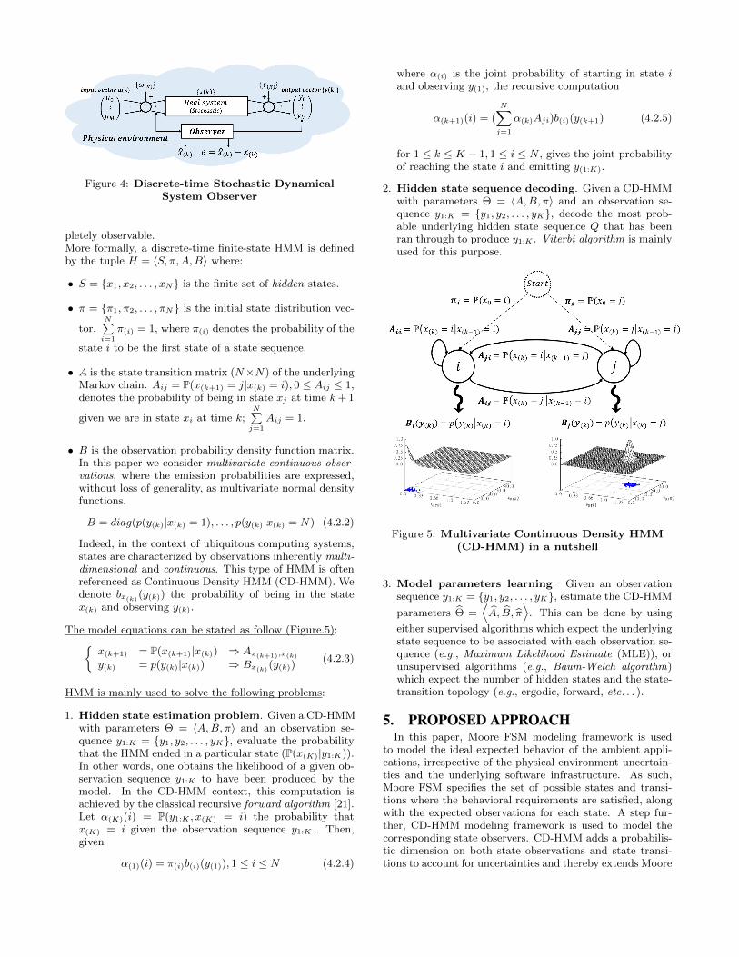
Figure 4: Discrete-time Stochastic DynamicalSystem Observer
pletely observable.More formally, a discrete-time finite-state HMM is definedby the tuple H = 〈S, π,A,B〉 where:
• S = {x1, x2, . . . , xN} is the finite set of hidden states.
• π = {π1, π2, . . . , πN} is the initial state distribution vec-
tor.N∑i=1
π(i) = 1, where π(i) denotes the probability of the
state i to be the first state of a state sequence.
• A is the state transition matrix (N×N) of the underlyingMarkov chain. Aij = P(x(k+1) = j|x(k) = i), 0 ≤ Aij ≤ 1,denotes the probability of being in state xj at time k+ 1
given we are in state xi at time k;N∑j=1
Aij = 1.
• B is the observation probability density function matrix.In this paper we consider multivariate continuous obser-vations, where the emission probabilities are expressed,without loss of generality, as multivariate normal densityfunctions.
B = diag(p(y(k)|x(k) = 1), . . . , p(y(k)|x(k) = N) (4.2.2)
Indeed, in the context of ubiquitous computing systems,states are characterized by observations inherently multi-dimensional and continuous. This type of HMM is oftenreferenced as Continuous Density HMM (CD-HMM). Wedenote bx(k)
(y(k)) the probability of being in the statex(k) and observing y(k).
The model equations can be stated as follow (Figure.5):{x(k+1) = P(x(k+1)|x(k)) ⇒ Ax(k+1),x(k)
y(k) = p(y(k)|x(k)) ⇒ Bx(k)(y(k))
(4.2.3)
HMM is mainly used to solve the following problems:
1. Hidden state estimation problem. Given a CD-HMMwith parameters Θ = 〈A,B, π〉 and an observation se-quence y1:K = {y1, y2, . . . , yK}, evaluate the probabilitythat the HMM ended in a particular state (P(x(K)|y1:K)).In other words, one obtains the likelihood of a given ob-servation sequence y1:K to have been produced by themodel. In the CD-HMM context, this computation isachieved by the classical recursive forward algorithm [21].Let α(K)(i) = P(y1:K , x(K) = i) the probability thatx(K) = i given the observation sequence y1:K . Then,given
α(1)(i) = π(i)b(i)(y(1)), 1 ≤ i ≤ N (4.2.4)
where α(i) is the joint probability of starting in state iand observing y(1), the recursive computation
α(k+1)(i) = (
N∑j=1
α(k)Aji)b(i)(y(k+1) (4.2.5)
for 1 ≤ k ≤ K − 1, 1 ≤ i ≤ N , gives the joint probabilityof reaching the state i and emitting y(1:K).
2. Hidden state sequence decoding. Given a CD-HMMwith parameters Θ = 〈A,B, π〉 and an observation se-quence y1:K = {y1, y2, . . . , yK}, decode the most prob-able underlying hidden state sequence Q that has beenran through to produce y1:K . Viterbi algorithm is mainlyused for this purpose.
Figure 5: Multivariate Continuous Density HMM(CD-HMM) in a nutshell
3. Model parameters learning. Given an observationsequence y1:K = {y1, y2, . . . , yK}, estimate the CD-HMM
parameters Θ =⟨A, B, π
⟩. This can be done by using
either supervised algorithms which expect the underlyingstate sequence to be associated with each observation se-quence (e.g., Maximum Likelihood Estimate (MLE)), orunsupervised algorithms (e.g., Baum-Welch algorithm)which expect the number of hidden states and the state-transition topology (e.g., ergodic, forward, etc. . . ).
5. PROPOSED APPROACHIn this paper, Moore FSM modeling framework is used
to model the ideal expected behavior of the ambient appli-cations, irrespective of the physical environment uncertain-ties and the underlying software infrastructure. As such,Moore FSM specifies the set of possible states and transi-tions where the behavioral requirements are satisfied, alongwith the expected observations for each state. A step fur-ther, CD-HMM modeling framework is used to model thecorresponding state observers. CD-HMM adds a probabilis-tic dimension on both state observations and state transi-tions to account for uncertainties and thereby extends Moore

FSM with viability zones [2], i.e. zones where the behavioralrequirements are satisfied, without necessarily being perfect(Figure.11). Therefore, Moore FSM dynamics ⊂ CD-HMMdynamics. The problem is then, given an ambient applica-tion whose ideal expected behavior is specified through aMoore FSM, to transform this model to its associated CD-HMM state observer further used to estimate the behavioraldrift of the concrete application against requirements fromobservations.
5.1 Moore FSM: A Probabilistic point of viewThe state transition function Γ maps a state x(k) ∈ S and
an input vector u(k) ∈ I to a next state x(k+1) ∈ S. This canbe traduced by (1) the probability of the input u(k) occur-rence and (2) the probability that this occurrence leads ef-fectively the state transition (joint probability). The outputfunction G maps each state to an output vector. Here again,
Figure 6: DFSA from a probabilistic point of view.uhold(k)
is the input leading the state to loop back on itself,and utrans(k)
is the input leading a transition from thestate x(k) to the state x(k+1)
this can be traduced by the probability of observing an out-put vector given the system is in a particular state (Figure6).Taking into account the input occurrence probability leadsthe apparition of a transient state where the output vectory(k) is partitioned with the input vector (Y(k) = (y(k), u(k))).It means that inputs have to be observed as part of the stateoutput vector. For a given Moore FSM, the probabilities dis-cussed above are implicit and values constrained as follow:
1. Input occurrence probability. Moore FSM doesn’tdefine an input occurrence function. The occurrence of aninput is exogenous to the model. So, from a probabilisticpoint of view, given a state x(k) ∈ S any input u(k) ∈ Imay occur at time k. This can be formulated as follow:
∀x(k) ∈ S,uM∑
u(k)=u1
Poccurrence(x(k), u(k)) = 1 (5.1.1)
2. State transition probability. The state transitionfunction Γ maps a state x(k) ∈ S and an input u(k) ∈ Ito the next state x(k+1) (x(k+1) = Γ(x(k), u(k))). Froma probabilistic standpoint, the Moore FSM implicit con-straint on state transitions can be stated as follow:∀x(k) ∈ S, u(k) ∈ I :
∃!x(k+1) ∈ S\Ptrans(x(k), x(k+1)|u(k)) = 1, (5.1.2a)xN∑
x(k+1)=x1
Ptrans(x(k), x(k+1)|u(k)) = 1, (5.1.2b)
xN∑x(k+1)=x1
Ptrans(x(k), x(k+1)) = 1 (5.1.2c)
Eq.5.1.2a is the probability for a transition to occur fromthe state x(k) ∈ S at time k to the state x(k+1) ∈ S at timek+1, given the occurrence of the input u(k) ∈ I at time k(joint probability). Eq.5.1.2a and Eq.5.1.2b put togetherstipulate that a couple x(k), u(k) at time k is associatedwith a unique state x(k+1) at time k + 1 (determinism).This constraint can be represented by a tri-dimensionalmatrix N × N × L. Interestingly, the probabilistic ap-proach describes all state transitions, even those not ex-plicitly described in the model (i.e., state transitions withprobability set to 0 in the N ×N × L matrix are implic-itly not accepted by the model). Eq.5.1.2c stipulates thatstate outgoing transitions are equiprobable. Indeed, in-puts being exogenous to the model, one cannot presumethe probability of the inputs occurrence to each other.
3. Output emission probability. Each state output vec-tor is given by y(k) = G(x(k)). From a probabilistic stand-point, the Moore FSM implicit constraints on outputs canbe stated as follow:∀x(k) ∈ S :
∃!y(k) ∈ Y \Pemission(y(k)|x(k)) = 1, (5.1.3a)yN∑
y(k)=y1
Pemission(y(k)|x(k)) = 1, (5.1.3b)
Eq.5.1.3a is the probability to emit y(k) ∈ Y given we arein the state x(k) ∈ S at time k. Eq.5.1.3a and Eq.5.1.3bput together stipulate that each state is associated witha unique output vector.
5.2 Moore FSM to CD-HMM projectionBased on the case-study described in section 2, let’s con-
sider an ambient application whose required behavior is de-fined by the Moore FSM depicted in Figure.7. The modeldescribes the ideal behavior of the ambient application thatcan be stated as follow:”While a human is present in the classroom, the luminosityof a point in space in the classroom must be maintained at30 lux. Otherwise, the luminosity must be maintained at 2lux”.
input u(k) Low luminosity(State 0)
High luminosity(State 1)
No presence (u = 0) Conform Non-conformPresence (u = 1) Non-conform Conform
Figure 7: Moore FSM Example.The luminosity of apoint in space must be set to 30 lux if human presence is
detected, 2 lux otherwise
This behavior can be modeled with two states: (1) whilebeing in the first state, i.e., no human presence is detected(u = 0), the expected luminosity is 2 lux (low luminosity,

represented by the output vector (00010)); (2) while be-ing in the second state, i.e., human presence is detected(u = 1), the expected luminosity is 30 lux (high luminosity,represented by the output vector (11110)). Let’s transformthese requirements to a CD-HMM state observer (definedby Θ = 〈A,B, π〉).
Construction of the state transition matrix (A). Weconsider the FSM model depicted in Figure.7 from a prob-abilistic point of view. First, we only consider the statetransitions probabilities and apply the constraints given byEqs.(5.1.2a, 5.1.2b and 5.1.2c). The resulting model is givenin Figure.8. For the time being, the state transitions are de-fined irrespective of the input. Without input information,the non-conform situations described in Figure.7 (i.e., (1)human presence is detected but the luminosity remains at alow level, (2) no human is detected but the luminosity is at ahigh level) cannot be detected because both states (i.e., lowand high luminosity) are defined by the model. Althoughboth states are defined by the model, they are conditionedby an input value. So, let’s now consider the input occur-rences probabilities as depicted in Figure.6. The resulting
Figure 8: Moore FSM from a probabilistic point ofview taking into account only the state transitions
probabilities
Figure 9: Moore FSM from a probabilistic point ofview taking into account both state transitions and
inputs occurrence probabilities
model is given in Figure.9. Transient states denote the factthat state transitions given in Figure.8 are conditioned byan input occurrence represented by the transient states inFigure.6.Note that in Figure.9, the state transitions from states 1→ 2and 4→ 0 are supposed to be instantaneous. Depending onthe observation sampling rate, there is a non-negligible prob-ability for a transient state to loop back on itself (i.e., theobservation values lead CD-HMM to consider that the appli-cation is still in the same state due to the observation prob-
ability density functions defined in matrix B). One need tointegrate this probability in the model, computed based onthe sensor data acquisition sampling rate. Also, some statesbeing equivalent (states 2/3 and 0/5), a model reduction canbe applied. The resulting model is given in Figure.10.Construction of the observation probabilities (B).Recall the definition of the matix B given by 4.2.2 wherep(y(k)|x(k)) are probability density functions expressed, with-out loss of generality, as multivariate normal density func-tions. Based on Figure.6, the observation vector is given by
Figure 10: Moore FSM from a probabilistic point ofview after states reduction
Y(k) = (y(k), u(k)), where y(k) is the luminosity sensor value∈ N and u(k) the human presence sensor value ∈ [0, 1]. Thusfor each x(k):
bx(k)(Y(k)) = p(Y(k)|x(k)) (5.2.1a)
=1√
(2π)n1√detΣ
e12
(Y(k)−µ)′Σ−1(Y(k)−µ)
(5.2.1b)
where n = 2 (Y(k) comprises two random variables, y(k) andu(k)), µ = E(Y(k)) an n-dimensional vector and Σ is then×n positive definite variance-covariance matrix of Y(k). µcan directly be retrieved from the Moore FSM model outputvectors. Variance and covariance values cannot be retrievedfrom the Moore FSM model directly and have to be definedoffline by the designer of the ambient application.Construction of the initial state distribution vector(π). The initial state distribution vector π is initialized withequiprobable values (πi = 1
N, 1 ≤ i ≤ N). Without setting
equiprobable values, the CD-HMM initial state distributionvector obtained from the Moore FSM depicted in Figure.10would be π = (π0 = 1.0, π1 = 0.0, π2 = 0.0, π3 = 0.0). Then,based on Eqs.(4.2.4 and 4.2.5), any observation sequencewhose initial state is not x0 would yield P(x(K)|y1:K) ≈ 0.0.Actually, one do not know the initial state of an observa-tion sequence gathered at any time from sensors. In otherwords, the starting state of an observation sequence can beany state x ∈ S.CD-HMM through parameters Θ = 〈A,B, π〉 adds a proba-bilistic dimension on both state emissions and state transi-tions to account for uncertainties and thereby extends MooreFSM with viability zones [2], i.e. zones where the behavioralrequirements of the ambient application are satisfied, with-out necessarily being perfect (e.g., the Figure.11 depicts via-bility zones defined from the observation probability densityfunctions defined in matrix B).

Figure 11: The CD-HMM observation matrix Bdefines viability zones through pdf
6. EVALUATION
6.1 Evaluation MethodologyThe following methodology has been used to evaluate the
validity of our approach:
1. Specify the ideal expected behavior of an ambientapplication as a Moore FSM. To this end, the finitestate machine designer tool Qfsm4 has been used.
2. Simulate the Moore FSM to obtain a set of traces.From the model, we developed Verilog test benches toproduce a set of traces as Value Change Dump (VCD)files (Figure.12). The length of the generated traces islimited to 350 events.
Figure 12: Example of a Moore FSM simulationwaveforms
3. Apply an additive random noise to the set of traces.We wrote a program that reads the set of traces obtainedfrom the simulation (.vcd) and transforms it to a Comma-Separated Values (.csv) dataset. A user defined addi-tive pseudo-random noise uniformly distributed has beenadded to the traces.
4. Transform the Moore FSM to its associated CD-HMM state observer, defined by Θ = 〈A,B, π〉. Weimplemented the algorithm described in section 5.2 totransform the Moore FSM model to its associated CD-HMM state observer. We used Accord.NET framework[20] to implement the CD-HMM engine.
5. Verify the CD-HMM state observer dynamics. Fromthe CD-HMM parameters Θ = 〈A,B, π〉, we generated
a probable observation sequence Y1:K (Figure.13). This
4urlhttp://qfsm.sourceforge.net/
step is necessary to ensure, offline, that the observer dy-namics is conform to the behavioral requirements of theambient application. Some parameters are then adjustedas necessary (variance-covariance matrix values and tran-sient states probabilities given the inputs acquisition sam-pling rate).
Figure 13: Observation sequence generated from theCD-HMM state observer depicted in Figure.10
6. Apply the set of traces as input to the CD-HMMstate observer. Given a CD-HMM state observer withparameters Θ = 〈A,B, π〉 and an observation sequenceY1:K = {Y1, Y2, . . . , YK}, one get the probability that theCD-HMM ended in a particular state (P(x(K)|y1:K)). Inother words, one obtains the likelihood of a given inputsequence Y1:K to have been produced by the model Θ =〈A,B, π〉.
6.2 Experimental ResultsWe applied the aforementioned methodology to the use-
case described in the Figure.7. We used MQTT (MessageQueuing Telemetry Transport) [10], a lightweight messag-ing protocol, to transmit each event of the set of traces tothe CD-HMM state observer on a regular basis (we set theemission rate to one event per second). We added a pseudo-random noise uniformly distributed between 0 and 0.2 to thetraces. Then, we set the observation window of the state ob-server to 10 events (Y1:K = {Y1, Y2, . . . , YK}, where K = 10and Y(k) = (y(k), u(k)), where y(k) is the luminosity sensorvalue ∈ N and u(k) the human presence sensor value ∈ [0, 1].The CD-HMM state observer is generated with a probabilityfor transient states to loop back on themselves set to 0.1. µvalues (Eq.5.2.1) are set from the Moore FSM output vec-tors for each state while the variance values of the matrixΣ are set to 0.02 and the covariance set to 0.0 (We considerindependent variables).We modified the set of traces to randomly introduce someviolations: (1) the luminosity in the classroom is degradedby some stochastic dynamics, (2) a second system preventsthe utilization of some devices (systems multiplicity and in-terferences).(1) Stochastic dynamics. In the first case, we simulateda situation where, while the observed ambient applicationis running, the weather turns cloudy. The drop in luminos-ity is detected by the luminosity sensor. The behavior ofthe ambient application starts drifting against requirements(blue curve in Figure.14). As the CD-HMM state observerreceives the observation sequence Y1:K = {Y1, Y2, . . . , YK}where K = 10, it detects the drift and returns negative log-likelihood values (red curve).

Figure 14: While the application is running, theweather turns cloudy. This leads a luminosity drop
Figure 15: Although a human is detected in theclassroom, the luminosity remains at a low level
(2) Systems multiplicity and interferences. In the sec-ond case we simulated a situation where, although a humanpresence is detected in the classroom (green curve in Fig-ure.15), the luminosity remains at a low level (blue curve).For instance, the ambient devices used in the first situation(some light bulbs) are disqualified by a second applicationmanaging the lighting power consumption. Here again, thenon-conformity of the behavior of the ambient applicationagainst requirements is detected by the CD-HMM state ob-server (red curve).
The magnitude of the quantification of the behavioral driftagainst the required behavior depends on the HMM param-
eters Θ = 〈A,B, π〉. Typically, if we compare the behavioralviolations previously depicted and associated drift quantifi-cations, in the first case (stochastic dynamics) the behavioris not expected at all by the model while in the second case(Systems multiplicity and interferences), the behavior is ex-pected but with low probability.
7. CONCLUSION AND FUTURE WORKThe proliferation of ambient devices in our physical sur-
roundings (a.k.a. connected objects) results in the simul-taneous presence of a large number of software services of-fered to the users. Their composition yields the so-calledambient applications whose primary objective is to smartlyand seamlessly assist users in their everyday lives, by off-loading them with the constraining physical and cognitivetasks. However, this vision, at the heart of smart-* sys-tems, is seriously hampered by the physical nature of theoperational environment the ambient applications operatein. Indeed, ambient devices interact in and through thephysical environment whose nature is intrinsically stochasticand subject to uncertainties that cannot be modeled entirelyoffline. Hence, apart from the case where the operational en-vironment is controlled or its future evolutions are known,any unforeseen environmental change (i.e., not modeled) canjeopardize the models and lead the behavior of the ambientapplications to drift over time.In this context, we have presented an approach providingsmart-* systems with the ability to quantify, at runtime,the behavioral drift of the ambient applications against re-quirements. The main idea of the proposed approach istwofold: (1) We modeled the ideal behavior of the ambientapplications as deterministic Moore Finite State Machines(Moore FSM). This modeling framework allows ambient ap-plications designers to specify: (i) the set of possible statesand state transitions in which the behavior of the ambi-ent applications is not compromised and (ii) the expectedobservations for each state. (2) We considered the MooreFSM modeling framework from a statistical point of view,and presented a framework to transform Moore FSM mod-els to their associated Continuous Density Hidden MarkovModel (CD-HMM) state observers. As such, HMM model-ing framework allows to take into account unertainties andextends Moore FSM with viability zones in which the be-havior of the ambient applications is not compromised. Wethen leveraged the ability of this modeling framework toestimate the likelihood of an observation sequence gatheredfrom sensors buried in the physical environment to have beenproduced by the model (i.e., the quantification of the behav-ioral drift against requirements).We validated our approach through a concrete use-case inthe field of school lighting. The results obtained demon-strate the soundness and efficiency of the proposed approachfor estimating the behavioral drifts of the ambient applica-tions at runtime in the presence of environmental distur-bances. In light of these results, we envision using this es-timation to support a decision-making algorithm within aself-adaptive system.To extend the application areas of the proposed approach,we plan to investigate cases where behavioral requirementshave to integrate temporal properties. For instance, we tar-get situations where ambient devices interactions could besubject to some temporal inertia (e.g., (1) in order to re-duce energy consumption, recent light bulbs reach their op-

timal luminosity after a given period of time; (2) a user re-quiring ambient temperature to be increased cannot expectthis requirement to be instantaneously executed). On thatfront, we plan to specify the required behaviors of the ambi-ent applications as discrete-time Finite State Time Machine(FSTM) [18] further transformed to Hidden Semi-MarkovModel (HSMM) state observer [25]. HSMM is said semi-Markov because the transition from a state x(k) to a subse-quent state x(k+1) does not only depend on the state x(k)
but also on its duration.Finally, the lack of experimental datasets covering the func-tional and non-functional behavioral aspects of the ambientapplications, makes difficult the benchmarking of differentapproaches. To fill the gap, we plan to gather datasets frommultiple fields ranging from assisted living to industry 4.0.
8. ACKNOWLEDGMENTSThis research was supported by GFI Informatique, Innova-tion Group.
9. REFERENCES[1] R. Alur. Principles of cyber-physical systems. MIT
Press, 2015.
[2] J.-P. Aubin, A. Bayen, and P. Saint-Pierre. ViabilityTheory: New Directions. Springer, 2011.
[3] N. Bencomo. Quantun: Quantification of uncertaintyfor the reassessment of requirements. In 23rdInternational Requirements Engineering Conference(RE), pages 236–240. IEEE, 2015.
[4] N. Bencomo and A. Belaggoun. A world full ofsurprises: Bayesian theory of surprise to quantifydegrees of uncertainty. In Companion Proceedings ofthe 36th International Conference on SoftwareEngineering, pages 460–463. ACM, 2014.
[5] N. Bencomo, R. France, B. Cheng, and U. Aßmann.Models@runtime: foundations, applications, androadmaps, volume 8378. Springer, 2014.
[6] R. Capilla, J. Bosch, P. Trinidad, A. Ruiz-Cortes, andA. Hinchey. An overview of dynamic software productline architectures and techniques: Observations fromresearch and industry. Journal of Systems andSoftware, 91:3 – 23, 2014.
[7] W. Chipman, C. Grimm, and C. Radojicic. Coverageof uncertainties in cyber-physical systems.GMM-Fachbericht-ZuE, 2015.
[8] R. de Lemos, D. Garlan, C. Ghezzi, and H. Giese.Software engineering for self-adaptive systems:Assurances (dagstuhl seminar 13511). DagstuhlReports, 3(12), 2014.
[9] H. Giese, N. Bencomo, L. Pasquale, A. J. Ramirez,P. Inverardi, S. Watzoldt, and S. Clarke. Living withuncertainty in the age of runtime models. InModels@runtime, pages 47–100. Springer, 2014.
[10] U. Hunkeler, H. L. Truong, and A. Stanford-Clark.MQTT- S A publish/subscribe protocol for wirelesssensor networks. In 2008 3rd International Conferenceon Communication Systems Software and Middlewareand Workshops (COMSWARE’08).
[11] V. Krishnamurthy. Partially Observed MarkovDecision Processes. Cambridge University Press, 2016.
[12] J. Krumm. Ubiquitous computing fundamentals. CRCPress, 2016.
[13] M. Kwiatkowska. Advances in quantitative verificationfor ubiquitous computing. In International Colloquiumon Theoretical Aspects of Computing, pages 42–58.Springer, 2013.
[14] M. Kwiatkowska. From software verification to’everyware’ verification. Computer Science-Researchand Development, 28(4):295–310, 2013.
[15] J. Nehmer, M. Becker, A. Karshmer, and R. Lamm.Living assistance systems: an ambient intelligenceapproach. In Proceedings of the 28th internationalconference on Software engineering, pages 43–50.ACM, 2006.
[16] M. Pinto, R. Almeida, P. Pinho, and L. Lemos.Daylighting in classrooms-the daylight factor as aperformance criterion. In ICEH-3rd InternationalCongress on Environmental Health, 2014.
[17] L. Rabiner. A tutorial on hidden markov models andselected applications in speech recognition. Proc.IEEE, 77(2):257–286, 1989.
[18] K. Sacha. Translatable finite state time machine. InInternational SDL Forum, pages 117–132. Springer,2007.
[19] I. Sarray, A. Ressouche, D. Gaffe, J.-Y. Tigli, andS. Lavirotte. Safe composition in middleware for theinternet of things. In Proceedings of the 2nd Workshopon Middleware for Context-Aware Applications in theIoT, pages 7–12. ACM, 2015.
[20] C. R. Souza. The accord.net framework, Dec 2014.http://accord-framework.net. Sao Carlos, Brazil.
[21] S. D. Stoller, E. Bartocci, J. Seyster, R. Grosu,K. Havelund, S. A. Smolka, and E. Zadok. Runtimeverification with state estimation. In InternationalConference on Runtime Verification, pages 193–207.Springer, 2011.
[22] G. Tamura, N. M. Villegas, H. A. Muller, J. P. Sousa,B. Becker, G. Karsai, S. Mankovskii, M. Pezze,W. Schafer, L. Tahvildari, et al. Towards practicalruntime verification and validation of self-adaptivesoftware systems. In Software Engineering forSelf-Adaptive Systems II, pages 108–132. Springer,2013.
[23] F. Wagner, R. Schmuki, T. Wagner, andP. Wolstenholme. Modeling software with finite statemachines: a practical approach. CRC Press, 2006.
[24] D. Weyns, N. Bencomo, R. Calinescu, J. Camara,C. Ghezzi, V. Grassi, L. Grunske, P. Inverardi, J.-M.Jezequel, S. Malek, et al. Perpetual assurances inself-adaptive systems. In Assurances for Self-AdaptiveSystems, Dagstuhl Seminar, volume 13511, 2014.
[25] S.-Z. Yu. Hidden semi-markov models. In Journal ofArtificial Intelligence, volume 174, pages 215–243,2010.
[26] M. Zhang, B. , Selic, S. Ali, T. Yue, O. Okariz, andR. Norgren. Understanding uncertainty incyber-physical systems: A conceptual model. InECMFA, 2016.
[27] X. Zheng, C. Julien, M. Kim, and S. Khurshid. On thestate of the art in verification and validation in cyberphysical systems. The University of Texas at Austin,The Center for Advanced Research in SoftwareEngineering, Tech. Rep. TR-ARiSE-2014-001, 2014.