on some electro-mechanical aspects of neuron model · discovery of nerve impulse flow from a squid...

OnsomeElectro-MechanicalAspectsofNeuronModel

BishakhBhattacharyaProfessor,DepartmentofMechanicalEngineering

IITKanpurKanpur208016

Brieforganizationofmypresentation

• Phase-I• ClassicalNeuronModelbasedonElectricPulseTransmission• ANewViewincorporatingMechanicalWavePropagation• SolitonPropagationinNerves• ABriefComparisonbetweenthetwomodels• CompromisingSolutionsintheHorizon• OpenIssues

• Phase-II• RevisitingBrainDynamicsfromtheperspectiveofnetworkedoscillation• InsearchofMetronomes• CanlearningbeintegratedwithDefaultModeNetwork?• ApplicationinChildRobotInteraction

DiscoveryofNerveImpulseflowfromaSquidGiantAxon

1. INTRODUCTION

The action potential is a propagating voltage pulse traveling along the

nerve axon. Since the first description of its electrical features by Luigi

Galvani [1] and Volta [2] in the past decade of the eighteenth century, its

nature has been in the focus of intense studies during the recent 200 years.

Starting from a famous paper by Bernstein [3] in 1902, it has been assumed

that the permeability of the neural membrane for ions is a necessary prereq-

uisite for the propagation of the nervous impulse in excitable membranes.

Bernstein based his considerations on the electrochemistry of semipermeable

walls, leading to a voltage difference across a membrane upon uneven dis-

tribution of positive and negative ions (Nernst potentials). While Bernstein

assumed that the permeability for ions breaks down in a nonspecific manner,

the later Hodgkin–Huxley (HH) model [4] is based on the assumption that

the membrane contains proteins that selectively conduct sodium and potas-

sium ions in a time- and voltage-dependent manner. This model was at the

basis of a rapid development in molecular biology, leading to numerous

studies on ion channel proteins. Until today, permeation studies on ion

channel proteins have been in the center of interest of molecular biology.

The HHmodel treats the nerve axon as an electrical circuit in which the

proteins are resistors and the membrane is a capacitor. Ion currents flow

through the membrane and along the nerve axon leading to a propagating

pulse. The voltage dependence of the channel proteins results a characteristic

spike (Fig. 9.1) described by a partial differential equation that exclusively

contains electrical parameters.While theHHmodel describes various aspects

of the action potential in a satisfactory manner (e.g., its velocity and the pulse

amplitude), it fails to describe several other aspects of the nerve pulse that are

Time (ms)Time (ms)

0 1 2 3 4 5 6 7 8 910

20

–0.5

0.0

0 100 200 300 400

0.5

40

60

80

0

100

Volta

ge (

mV

)

Volta

ge (

mV

)

Figure 9.1 The action potential. Left: The action potential in a squid axon, adapted fromRef. [5]. Right: Extracellular recording of action potential from grasshopper nerves.Adapted from Ref. [6].

276 Revathi Appali et al.

HodgkinandHuxley1952

Thelargesizeofthesquidgiantaxonisaspecializationforrapidconductionofactionpotentialsthattriggerthecontractionofthesquid’smantlewhenescapingfromapredator.Inadditiontobeingbeneficialforthesquid,thelargediameterofthegiantaxonwasbeneficialforHodgkinandHuxleybecauseitpermittedmanipulationsthatwerenottechnicallyfeasibleinsmalleraxonsthathadbeenusedinbiophysicalstudiesuptothatpoint.

TheActionPotentialinaSquidAxon[1]andExtracellularRecordingsfromGrasshopperNerves

TheHodgkinandHuxleyModel

• Signaltravelsthroughnervefibres ofGiantSquidataspeedupto30m/swhichisabout108km/hr

[Forhuman:Musclefibre control425km/hr,Touch– 274km/hr,Pain–2.2Km/hr]• Byfixingelectrodesintonervecells(VoltageClamp),itisdiscoveredthatasanervepulsetravelsandpassestheelectrode,avoltagespikeoccursforseveralthousandthsofasecond.• Further,thecauseofvoltagespikewasattributedtothestreamingoutofSodiumionsfromthechannelfollowedbypotassiumionsguessinginsideduetowhichsoonafterthevoltagesubsides.

TheH-HElectricalModel

• Inbiophysicsbasedneuralmodeling,theelectricalpropertiesofaneuronarerepresentedintermsofanelectricalequivalentcircuit.• Capacitorsareusedtomodelthechargestoragecapacityofthecellmembrane• Resistorsareusedtomodelthevarioustypesofionchannelsembeddedinmembrane• Batteriesareusedtorepresenttheelectrochemicalpotentialsestablishedbydifferingintra- andextracellularionconcentrations.

TheCircuitDiagram

• The capacitive current 𝐼" is defined by the rate of change of charge q at the membrane surface: 𝐼" = dq/dt.The charge q(t) is related to the instantaneous membrane voltage 𝑉$(t) and membrane capacitance 𝐶$ bythe relationship 𝑞 = 𝐶$𝑉$.

• the ionic current 𝐼)*+ is subdivided into three distinct components, a sodium current 𝐼,-, a potassiumcurrent 𝐼., and a small leakage current 𝐼/ that is primarily carried by chloride ions, The pathway labeled“stim” represents an externally applied current, such as might be introduced via an intracellular electrode.

Nelson, M.E. (2004) Electrophysiological Models In: Databasing the Brain: From Data to Knowledge. (S. Koslow and S. Subramaniam, eds.) Wiley, New York.

current IK, and a small leakage current IL that is primarily carried by chloride ions. The behavior of an electrical circuit of the type shown in Fig. 1 can be described by a differential equation of the general form:

extionm

m IIdt

dVC =+ (1)

where Iext is an externally applied current, such as might be introduced through an intracellular electrode. Equation 1 is the fundamental equation relating the change in membrane potential to the currents flowing across the membrane.

Macroscopic Ionic Currents

The individual ionic currents INa, IK and IL shown in Fig. 1 represent the macroscopic currents flowing through a large population of individual ion channels. In HH-style models, the macroscopic current is assumed to be related to the membrane voltage through an Ohm’s law relationship of the form V=IR. In many cases it is more convenient to express this relationship in terms of conductance rather than resistance, in which case Ohm’s law becomes I = GV, where the conductance G is the inverse of resistance, G = 1/R. In applying this relationship to ion channels, the equilibrium potential Ek for each ion type also needs to be taken into account. This is the potential at which the net ionic current flowing across the membrane would be zero. The equilibrium potentials are represented by the batteries in Fig. 1. The current is proportional to the

Fig. 1 Electrical equivalent circuit for a short segment of squid giant axon. The capacitor represents the capacitance of the cell membrane; the two variable resistors represent voltage-dependent Na+ and K+

conductances, the fixed resistor represents a voltage-independent leakage conductance and the three batteries represent reversal potentials for the corresponding conductances. The pathway labeled “stim” represents an externally applied current, such as might be introduced via an intracellular electrode. The sign conventions for the various currents are indicated by the directions of the corresponding arrows. Note that the arrow for the external stimulus current Iext is directed from outside to inside (i.e., inward stimulus current is positive), whereas arrows for the ionic currents INa, IK and IL are directed from inside to outside (i.e., outward ionic currents are positive). After Hodgkin & Huxley (1952).

Thegoverningequations• Thebehaviouroftheelectriccircuitmaybegovernedbythefollowingequation:

• where𝐼012 isanexternallyappliedcurrent,suchasmightbeintroducedthroughanintracellularelectrode.

• Thetotalioniccurrent𝐼)*+ isthealgebraicsumoftheindividualcontributionsfromallparticipatingchanneltypesfoundinthecellmembrane suchthat:

• TheIoniccurrentisproportionaltoconductancetimesthedifferencebetweenthemembranepotential𝑉$andtheequilibriumpotential𝐸4.


current IK, and a small leakage current IL that is primarily carried by chloride ions. The behavior of an electrical circuit of the type shown in Fig. 1 can be described by a differential equation of the general form:

extionm

m IIdt

dVC =+ (1)

where Iext is an externally applied current, such as might be introduced through an intracellular electrode. Equation 1 is the fundamental equation relating the change in membrane potential to the currents flowing across the membrane.

Macroscopic Ionic Currents

The individual ionic currents INa, IK and IL shown in Fig. 1 represent the macroscopic currents flowing through a large population of individual ion channels. In HH-style models, the macroscopic current is assumed to be related to the membrane voltage through an Ohm’s law relationship of the form V=IR. In many cases it is more convenient to express this relationship in terms of conductance rather than resistance, in which case Ohm’s law becomes I = GV, where the conductance G is the inverse of resistance, G = 1/R. In applying this relationship to ion channels, the equilibrium potential Ek for each ion type also needs to be taken into account. This is the potential at which the net ionic current flowing across the membrane would be zero. The equilibrium potentials are represented by the batteries in Fig. 1. The current is proportional to the

Fig. 1 Electrical equivalent circuit for a short segment of squid giant axon. The capacitor represents the capacitance of the cell membrane; the two variable resistors represent voltage-dependent Na+ and K+

conductances, the fixed resistor represents a voltage-independent leakage conductance and the three batteries represent reversal potentials for the corresponding conductances. The pathway labeled “stim” represents an externally applied current, such as might be introduced via an intracellular electrode. The sign conventions for the various currents are indicated by the directions of the corresponding arrows. Note that the arrow for the external stimulus current Iext is directed from outside to inside (i.e., inward stimulus current is positive), whereas arrows for the ionic currents INa, IK and IL are directed from inside to outside (i.e., outward ionic currents are positive). After Hodgkin & Huxley (1952).


conductance times the difference between the membrane potential Vm and the equilibrium potential Ek. The total ionic current Iion is the algebraic sum of the individual contributions from all participating channel types found in the cell membrane:

∑∑ −==k

kmkk

kion EVGII )( (2)

which expands to the following expression for the Hodgkin-Huxley model of the squid axon:

)()()( LmLKmKNamNaion EVGEVGEVGI −+−+−= (3)

Note that individual ionic currents can be positive or negative depending on whether or not the membrane voltage is above or below the equilibrium potential. This raises the question of sign conventions. Is a positive ionic current flowing into or out of the cell? The most commonly used sign convention in neural modeling is that ionic current flowing out of the cell is positive and ionic current flowing into the cell is negative (see subsection on Sign Conventions for more details).

In general, the conductances are not constant values, but can depend on other factors like the membrane voltage or the intracellular calcium concentration. In order to explain their experimental data, Hodgkin and Huxley postulated that GNa and GK were voltage-dependent quantities, whereas the leakage current GL was taken to be constant. Thus the resistor symbols in Fig. 1 are shown as variable resistors for GNa and GK, and as a fixed resistor for GL. Today, we know that the voltage-dependence of GNa and GK can be related to the biophysical properties of the individual ion channels that contribute to the macroscopic conductances. Although Hodgkin and Huxley did not know about the properties of individual membrane channels when they developed their model, it will be convenient for us to describe the voltage-dependent aspects of their model in those terms.

Gates

The macroscopic conductances of the HH model can be considered to arise from the combined effects of a large number of microscopic ion channels embedded in the membrane. Each individual ion channel can be thought of as containing one or more physical gates that regulate the flow of ions through the channel. An individual gate can be in one of two states, permissive or non-permissive. When all of the gates for a particular channel are in the permissive state, ions can pass through the channel and the channel is open. If any of the gates are in the non-permissive state, ions cannot flow and the channel is closed. Although it might seem more natural to speak of gates as being open or closed, a great deal of confusion can be avoided by consistently using the terminology permissive and non-permissive for gates while reserving the terms open and closed for channels.

The voltage-dependence of ionic conductances is incorporated into the HH model by assuming that the probability for an individual gate to be in the permissive or non-permissive state depends on the value of the membrane voltage. If we consider gates of a particular type i, we can define a probability pi, ranging between 0 and 1, which represents the probability of an individual gate being in the permissive state. If we consider a large number of channels, rather than an individual channel, we can also interpret pi as the fraction of gates in that population that

ThevariationofConductancewithGate

• ThemacroscopicconductanceoftheHHmodelcanbeconsideredtoarisefromthecombinedeffectsofalargenumberofmicroscopicionchannelsembeddedinthemembrane.• Eachindividualionchannelcanbethoughtofascontainingoneormorephysicalgatesthatregulatetheflowofionsthroughthechannel.Anindividualgatecanbeinoneoftwostates,permissiveornon-permissive.• Atsomepointintimet,let𝑝)(t) representthefractionofgatesthatareinthepermissivestate.Consequently1- 𝑝) (t)mustbeinthenon-permissivestate.

ProbabilisticVariationoftheGate

• Theprobabilisticvariationintermsofrateconstant:

• Thetransitionbetweenthepermissiveandnon-permissivestatesareassumedtoobeyfirstorderkineticsasfollows:

• Thesteadystatevalue:withtimeconst.


are in the permissive state. At some point in time t, let pi(t) represent the fraction of gates that are in the permissive state. Consequently 1- pi (t) must be in the non-permissive state.

)(,(1, )(

)(

t pstatepermissive

nfraction i

t)p statepermissivenon

nfraction i

iV

V

ii

i

← →

−−

β

α

The rate at which gates transition from the non-permissive state to the permissive state is denoted by a variable αi(V), which has units of sec-1. Note that this “rate constant” is not really constant, but depends on membrane voltage V. Similarly there is a second rate constant, β i(V) describing the transition rate from the permissive to the non-permissive state. Transitions between permissive and non-permissive states in the HH model are assumed to obey first-order kinetics:

iiiii pVpV

dtdp )()1)(( βα −−= (4)

where αi(V) and β i(V) are voltage-dependent. If the membrane voltage Vm is clamped at some fixed value V, then the fraction of gates in the permissive state will eventually reach a steady state value (i.e., dpi/dt = 0) as t‡8 given by:

)()()(

, VVVp

ii

iti βα

α+

=∞→ (5)

The time course for approaching this equilibrium value is described by a simple exponential with time constant τi(V) given by:

)()(1)(

VVV

iii βατ

+= (6)

When an individual channel is open, it contributes some small, fixed value to the total conductance and zero otherwise. The macroscopic conductance for a large population of channels is thus proportional to the number of channels in the open state, which is in turn proportional to the probability that the associated gates are in their permissive state. Thus the macroscopic conductance Gk due to channels of type k, with constituent gates of type i, is proportional to the product of the individual gate probabilities pi:

∏=i

ikk pgG (7)

where kg is a normalization constant that determines the maximum possible conductance when all the channels are open (i.e. all gates are in the permissive state).

We have presented Eqs. 4–7 using a generalized notation that can be applied to a wide variety of conductances beyond those found in the squid axon. To conform to the standard notation of the HH model, the probability variable pi in Eqs. 4–7 is replaced by a variable that represents the gate type. For example, Hodgkin and Huxley modeled the sodium conductance



)(,(1, )(

)(

t pstatepermissive

nfraction i


nfraction i

iV

V

ii

i

← →

−−

β

α


iiiii pVpV

dtdp )()1)(( βα −−= (4)


)()()(

, VVVp

ii

iti βα

α+

=∞→ (5)


)()(1)(

VVV

iii βατ

+= (6)


∏=i

ikk pgG (7)





)(,(1, )(

)(

t pstatepermissive

nfraction i


nfraction i

iV

V

ii

i

← →

−−

β

α


iiiii pVpV

dtdp )()1)(( βα −−= (4)


)()()(

, VVVp

ii

iti βα

α+

=∞→ (5)


)()(1)(

VVV

iii βατ

+= (6)


∏=i

ikk pgG (7)





)(,(1, )(

)(

t pstatepermissive

nfraction i


nfraction i

iV

V

ii

i

← →

−−

β

α


iiiii pVpV

dtdp )()1)(( βα −−= (4)


)()()(

, VVVp

ii

iti βα

α+

=∞→ (5)


)()(1)(

VVV

iii βατ

+= (6)


∏=i

ikk pgG (7)



TheConductancevsGaterelationship


using three gates of a type labeled “m” and one gate of type “h”. Applying Eq. 7 to the sodium channel using both the generalized notation and the standard notation yields:

hmgppgG NahmNaNa33 == (8)

Similarly, the potassium conductance is modeled with 4 identical “n” gates:

44 ngpgG NanKK == (9)

Summarizing the ionic currents in the HH model in standard notation, we have:

)()()( 43LmLKmKNamNaion EVgEVngEVhmgI −+−+−= (10)

mVmVdtdm

mm )()1)(( βα −−= (11)

hVhVdtdh

hh )()1)(( βα −−= (12)

nVnVdtdn

nn )()1)(( βα −−= (13)

To completely specify the model, the one task that remains is to specify how the six rate constants in Eqs. 11–13 depend on the membrane voltage. Then Eqs. 10–13, together with Eq. 1, completely specify the behavior of the membrane potential Vm in the HH model of the squid giant axon.

Sign Conventions

Note that the appearance of Iion on the left-hand side of Eq. 1 and Iext on the right indicates that they have opposite sign conventions. As the equation is written, a positive external current Iext will tend to depolarize the cell (i.e., make Vm more positive) while a positive ionic current Iion will tend to hyperpolarize the cell (i.e., make Vm more negative). This sign convention for ionic currents is sometimes referred to as the neurophysiological or physiologists’ convention. This convention is conveniently summarized by the phrase “inward negative”, meaning that an inward flow of positive ions into the cell is considered a negative current. This convention perhaps arose from the fact that when one studies an ionic current in a voltage clamp experiment, rather than measuring the ionic current directly, one actually measures the clamp current which is necessary to counterbalance it. Thus an inward flow of positive ions is observed as a negative-going clamp current, hence explaining the “inward negative” convention. Some neural simulation software packages, such as GENESIS, use the opposite sign convention (inward positive), since that allows all currents to be treated consistently. In the figures shown in this chapter, membrane currents are plotted using the neurophysiological convention (inward negative).








mVmVdtdm

mm )()1)(( βα −−= (11)

hVhVdtdh

hh )()1)(( βα −−= (12)

nVnVdtdn

nn )()1)(( βα −−= (13)


Sign Conventions









mVmVdtdm

mm )()1)(( βα −−= (11)

hVhVdtdh

hh )()1)(( βα −−= (12)

nVnVdtdn

nn )()1)(( βα −−= (13)


Sign Conventions



2 by finding values of )( cVn∞ , )0(∞n , and )( cn Vτ that give the best fit to the data for each value of Vc. Fig. 3 illustrates this process, using some simulated conductance data generated by the Hodgkin-Huxley model. Recall that n takes on values between 0 and 1, so in order to fit the conductance data, n must be multiplied by a normalization constant Kg that has units of conductance. For simplicity, the normalized conductance KK gG / is plotted. The dotted line in Fig. 3 shows the best-fit results for a simple exponential curve of the form given in Eq. 17. While this simple form does a reasonable job of capturing the general time course of the conductance change, it fails to reproduce the sigmoidal shape and the temporal delay in onset. This discrepancy is most apparent near the onset of the conductance change, shown in the inset of Fig. 3. Hodgkin and Huxley realized that a better fit could be obtained if they considered the conductance to be proportional to a higher power of n. Figure 3 shows the results of fitting the conductance data using a form j

kK ngG = with powers of j ranging from 1 to 4. Using this sort of fitting procedure, Hodgkin and Huxley determined that a reasonable fit to the K+ conductance data could be obtained using an exponent of j=4. Thus they arrived at a description for the K+ conductance under voltage clamp conditions given by:

[ ]4/4 ))0()(()( ntccKKK enVnVngngG τ−

∞∞∞ −−== (18)

Fig. 3 Best fit curves of the form j

Kk ngG = (j = 1–4) for simulated conductance vs. time data. The inset shows an enlargement of the first millisecond of the response. The initial inflection in the curve cannot be well-fit by a simple exponential (dotted line) which rises linearly from zero. Successively higher powers of j (j=2: dot-dashed; j=3: dashed line) result in a better fit to the initial inflection. In this case, j=4 (solid line) gives the best fit.


Activation and Inactivation gates

The strategy Hodgkin and Huxley used for modeling the sodium conductance is similar to that described above for the potassium conductance, except that the sodium conductance shows a more complex behavior. In response to a step change in clamp voltage, the sodium conductance exhibits a transient response (Fig. 4), whereas the potassium conductance exhibits a sustained response (Fig. 2). Sodium channels inactivate whereas the potassium channels do not. To model this process, Hodgkin and Huxley postulated that the sodium channels had two types of gates, an activation gate, which they labeled m, and an inactivation gate, which they labeled h. Again, boundary conditions dictated that m and h must follow a time course given by:

)(/))0()(()()( cm Vtcc emVmVmtm τ−

∞∞∞ −−= (19)

)(/))0()(()()( ch Vtcc ehVhVhth τ−

∞∞∞ −−= (20)

Hodgkin and Huxley made some further simplifications by observing that the sodium conductance in the resting state is small compared to the value obtained during a large depolarization, hence they were able to neglect )0(∞m in their fitting procedure. Likewise, steady state inactivation is nearly complete for large depolarizations, so )( cVh∞ could also be eliminated

Fig. 4 Simulated voltage-clamp data illustrating activation and inactivation properties of the Na+ conductance in squid giant axon. The command voltage Vc is shown in the lower panel and the Na+ current in the upper panel. Simulation parameters are from the Hodgkin and Huxley model (1952).

PropertiesunexplainedbytheH-Hmodel

•Whynervesdisplaythicknessandlengthvariationsundertheinfluenceoftheactionpotential?•Whytheactionpotentialcanbeexcitedbyamechanicalstimulus?•Whyduringthefirstphaseofthenervepulse,heatisreleasedfromthemembrane,whileitisreabsorbedduringthesecondphase• Itseemsasifthemechanicalandtheheatsignaturesratherindicatethatthenervepulseisanadiabaticandreversiblephenomenonsuchasthepropagationofamechanicalwave.

DevelopmentofaNewModel

• ConsiderthewellknownEulerwaveequationforareadensity∆𝜌8 as:

• However,closetothemeltingtransition,thevelocityofsound,cisnotconstantanditmaybewrittenas(‘p’,‘q’arematerialparameters).Also,consideringdispersionofsoundwaveintoaccount.

maximum.This implies that the lateral compressionof a fluidmembrane leads

to an increase in compressibility. This effect is known as a nonlinearity. From

experiment, it is known that the compressibility is also frequency dependent,

an effect that is known as dispersion. These two phenomena are necessary

conditions for the propagation of solitons. It can be shown that the features

of lipid membranes slightly above a transition are sufficient to allow the

propagation of mechanical solitons along membrane cylinders [21]. The

solitons consists of a reversible compression of the membrane that is linked

to a reversible release of heat, mechanical changes in the membrane.

Furthermore, the soliton model also implies a mechanism for anesthesia

that lies in the well-understood influence that anesthetics have on the lipid

phase transition [38].

The soliton model starts with the well-known wave equation for area

density changes DrA

@2

@t2DrA ¼ @

@zc2

@

@zDrA

! "ð9:9Þ

that originates from the Euler equations of compressible media (e.g.,

[39,40]). Here, t is the time, z is the position along the nerve axon, and c

is the sound velocity. If c¼ c0 is constant, one finds the relation for sound

propagation (@ 2r/@ t2)¼ c02(@ 2r/@ z2).

However, it has been shown that close to melting transitions in mem-

branes, the sound velocity is a sensitive function of density [41,42]. As

shown in Fig. 9.5, such transitions are found in biomembranes. This is

taken into account by expanding the sound velocity around its value in

the fluid phase

c2 ¼ c20 þpDrAþ qðDrAÞ2þ%%% ð9:10Þ

up to terms of quadratic order. The parameters p and q describe the depen-

dence of the sound velocity on density close to the melting transition and are

fitted to experimental data [21].

It is further known that the speed of sound is frequency dependent. This

effect is known as dispersion. In order to take dispersion into account, a sec-

ond term is introduced into Eq. (9.9) that assumes the form:

& h@4

@z4DrA ð9:11Þ

where h is a constant. For low-amplitude sound, this term leads to the

most simple dispersion relation c2¼ c02þ (h/c0

2)o2¼ c02þconst %o2. Lacking

285Comparison of the Hodgkin–Huxley Model and the Soliton Theorymaximum.This implies that the lateral compressionof a fluidmembrane leads

to an increase in compressibility. This effect is known as a nonlinearity. From

experiment, it is known that the compressibility is also frequency dependent,

an effect that is known as dispersion. These two phenomena are necessary

conditions for the propagation of solitons. It can be shown that the features

of lipid membranes slightly above a transition are sufficient to allow the

propagation of mechanical solitons along membrane cylinders [21]. The

solitons consists of a reversible compression of the membrane that is linked

to a reversible release of heat, mechanical changes in the membrane.

Furthermore, the soliton model also implies a mechanism for anesthesia

that lies in the well-understood influence that anesthetics have on the lipid

phase transition [38].

The soliton model starts with the well-known wave equation for area

density changes DrA

@2

@t2DrA ¼ @

@zc2

@

@zDrA

! "ð9:9Þ

that originates from the Euler equations of compressible media (e.g.,

[39,40]). Here, t is the time, z is the position along the nerve axon, and c

is the sound velocity. If c¼ c0 is constant, one finds the relation for sound

propagation (@ 2r/@ t2)¼ c02(@ 2r/@ z2).

However, it has been shown that close to melting transitions in mem-

branes, the sound velocity is a sensitive function of density [41,42]. As

shown in Fig. 9.5, such transitions are found in biomembranes. This is

taken into account by expanding the sound velocity around its value in

the fluid phase

c2 ¼ c20 þpDrAþ qðDrAÞ2þ%%% ð9:10Þ

up to terms of quadratic order. The parameters p and q describe the depen-

dence of the sound velocity on density close to the melting transition and are

fitted to experimental data [21].

It is further known that the speed of sound is frequency dependent. This

effect is known as dispersion. In order to take dispersion into account, a sec-

ond term is introduced into Eq. (9.9) that assumes the form:

& h@4

@z4DrA ð9:11Þ

where h is a constant. For low-amplitude sound, this term leads to the

most simple dispersion relation c2¼ c02þ (h/c0

2)o2¼ c02þconst %o2. Lacking

285Comparison of the Hodgkin–Huxley Model and the Soliton Theory

good data on the frequency dependence of sound in the kilohertz regime,

the term given by Eq. (9.11) is most natural dispersion term.

Combining Eqs. (9.9)–(9.11) leads to the final time and position-

dependent partial differential equation [21,23]:

@2

@t2DrA¼ @

@zc20 þpDrAþ qðDrAÞ2þ%% %! " @

@zDrA

# $& h

@4

@z4DrA ð9:12Þ

which describes the propagation of a longitudinal density pulse in a myelin-

ated nerve. In this equation,

• DrA is the change in lateral density of the membrane DrA¼rA & r0A;

• rA is the lateral density of the membrane;

• r0A is the equilibrium lateral density of the membrane in the fluid phase;

• c0 is the velocity of small-amplitude sound;

• p and q are the parameters determined from density dependence of the

sound velocity. These two constants parameterize the experimental

shape of the melting transition of the membrane and are given in Ref.

[21];

• h is a parameter describing the frequency dependence of the speed of

sound, that is, the dispersion.

All parameters except h are known from experiment. The empirical equi-

librium value of r0A is 4.035 ' 10& 3g/m2, and the low-frequency sound

velocity c0 is 176.6m/s. The coefficients p and q were fitted to measured

values of the sound velocity as a function of density. The parameter h is

not known experimentally due to difficulties to measure the velocity of

sound in the kilohertz regime. However, Chapter 2 attempts to derive this

parameter theoretically from relaxation measurements.

The nonlinearity and dispersive effects of the lipids can produce a self-

sustaining and localized density pulse (soliton) in the fluid membrane (see

Fig. 9.6). The pulse consists of a segment of the membrane that locally is

found in a solid (gel) state. It preserves its amplitude, shape, and velocity

while propagating along the nerve axon. Further, the pulse propagates over

long distances without loss of energy.

In the following, we work with the dimensionless variables u (dimen-

sionless density change), x, and t defined in Ref. [23] as

u¼DrA

rA0; x¼ c0

hz; t¼ c20ffiffiffi

hp t; B1¼

r0c20p; B2¼

r20c20q ð9:13Þ


Dispersion

Non-dimensionalisation ofthewaveequation:





@2

@t2DrA¼ @


@zDrA

# $& h

@4

@z4DrA ð9:12Þ










[21];


















u¼DrA

rA0; x¼ c0


hp t; B1¼

r0c20p; B2¼

r20c20q ð9:13Þ






@2

@t2DrA¼ @


@zDrA

# $& h

@4

@z4DrA ð9:12Þ










[21];


















u¼DrA

rA0; x¼ c0


hp t; B1¼

r0c20p; B2¼

r20c20q ð9:13Þ


Equation (9.12) now assumes the following form:

@2u

@t2¼ @

@xðBðuÞÞ@u

@x$ @4u

@x4ð9:14Þ

with

BðuÞ¼ 1 þ B1u þ B2u2 ð9:15Þ

B1¼$ 16.6 and B2¼79.5 were determined experimentally for a syn-

thetic lipid membrane in Ref. [21]. If we consider a density pulse u prop-

agating with constant velocity, we can use the coordinate transformation

x¼x $ bt (where b is the dimensionless propagation velocity of the density

pulse) and we yield the following form:

b2@2u

@x2¼ @

@xBðuÞ@u

@x

! "$ @4u

@x4ð9:16Þ

This is very much in the spirit of Eq. (9.7) used to obtain a propagating

solution. Equation (9.15) displays exponentially localized solitary solutions

which propagate without distortion for a finite range of subsonic velocities

[21,23].

Time (ms)0.0

0.0

0.00

DrA

/r0A

0.05

0.10

0.15

0.20

0.1 0.2 0.3 0.4

0.5 1.0 1.5 2.0 2.5 3.0

z (m)

Figure 9.6 Calculated solitary density pulse as a function of lateral position calculatedusing experimental parameters for a synthetic membrane. The pulse travels with about100 m/s. From Ref. [43].


Modifiedequationconsideringthepropagationofdensitypulse• Considerthepropagationofthedensitypulse‘u’withaconstantvelocity.• Wecanuseacoordinatetransformation𝜉 = 𝑥 − 𝛽𝑡,where𝛽 isthedimensionlesspropagationofvelocitywhichgivesusthemodifiedequationas:


@2u

@t2¼ @

@xðBðuÞÞ@u

@x$ @4u

@x4ð9:14Þ

with







b2@2u

@x2¼ @

@xBðuÞ@u

@x

! "$ @4u

@x4ð9:16Þ




[21,23].

Time (ms)0.0

0.0

0.00

DrA

/r0A

0.05

0.10

0.15

0.20

0.1 0.2 0.3 0.4

0.5 1.0 1.5 2.0 2.5 3.0

z (m)



TheanalyticalsolutionofthedensitypropagationequationThe above differential equation possesses analytical solutions given by

uðxÞ ¼ 2aþa%

ðaþþ a% Þþðaþ % a% Þcoshðxffiffiffiffiffiffiffiffiffiffiffiffiffiffi1 % b2Þ

q ð9:17Þ

where u ¼ a& is given by

a& ¼ % B1

B21 &

ffiffiffiffiffiffiffiffiffiffiffiffiffiffiffib2 % b201 % b20

s !

ð9:18Þ

for the velocity range b0<|b|<1 (with 1 being the low-amplitude sound

velocity). There exists a lower limit for the propagation velocity of the pulse

given by b0 ¼ 0.649851 for a synthetic membrane. No solitons exist

for slower velocities. The density change u(x) describes the shape of the

propagating soliton, which depends on the velocity b. A typical soliton

generated by Eq. (9.16) is shown in Fig. 9.6. The minimum propagation

velocity b is about 100 m/s, very similar to the measured propagation

velocity of the action potential inmyelinated nerves. Since the pulse describes

a reversible mechanical pulse, it possesses a reversible heat production, a

thickening and a simultaneous shortening of the nerve axon, in agreement

with observation. Due to the electrostatic features of biomembranes,

the pulse possesses a voltage component. Thus, the traveling soliton can

be considered a piezoelectric pulse.

One feature of the solitonmodel not discussed here in detail is that it pro-

vides a mechanism for general anesthesia. It has been shown that general

anesthetics lower the melting points of lipid membranes. At critical dose

(where 50% of the individuals are anesthetized), the magnitude of this shift

is independent of the chemical nature of the anesthetic drugs [38,44].

From this, one can deduce quantitatively how much free energy is

required to trigger a soliton. In the presence of anesthetics, this free energy

requirement is higher. As a result, nerve pulse stimulation is inhibited.

In this respect, it is interesting to note that hydrostatic pressure reverses

anesthesia. For instance, tadpoles anesthetized by ethanol wake up at

pressures around 50 bars [45]. It is also known that hydrostatic pressure

increases melting temperatures of lipid membranes due to the positive excess

volume of the transition [46]. The effects of anesthetics and hydrostatic

pressure are known quantitatively. Therefore, one can also quantitatively

calculate at what pressure the effect of anesthetics is reversed. The resulting

pressures are of the order of 25 bars at critical anesthetic dose, which is of

same order than the observed pressure reversal of anesthesia [19,38].


The above differential equation possesses analytical solutions given by

uðxÞ ¼ 2aþa%


q ð9:17Þ


a& ¼ % B1

B21 &


s !

ð9:18Þ
































The above differential equation possesses analytical solutions given by

uðxÞ ¼ 2aþa%


q ð9:17Þ


a& ¼ % B1

B21 &


s !

ð9:18Þ
































Thevalueofnon-dimensionalvelocity,𝛽 generallyliesbetween0.6to1

Thisiswhatthesolutionlookslike:


@2u

@t2¼ @

@xðBðuÞÞ@u

@x$ @4u

@x4ð9:14Þ

with







b2@2u

@x2¼ @

@xBðuÞ@u

@x

! "$ @4u

@x4ð9:16Þ




[21,23].

Time (ms)0.0

0.0

0.00

DrA

/r0A

0.05

0.10

0.15

0.20

0.1 0.2 0.3 0.4

0.5 1.0 1.5 2.0 2.5 3.0

z (m)



ItisaSoliton!

Asoliton isaself-reinforcingsolitarywavepacketthatmaintainsitsshapewhileitpropagatesataconstantvelocity.

Thesearecausedbyacancellationofnonlinearanddispersiveeffectsina medium.Thesolitonphenomenonwasfirstdescribedin1834byJohnScottRussellwhoobservedasolitarywaveintheUnionCanalinScotland.

GeneratingSolitonsinReal-life

Whathappenswhenthesoliton’scollide?

• IthasbeenshownbyTasakithatNervepulsesareblockeduponcollision.• AccordingtoHHmodel,propagationofanervepulsegeneratearefractoryperiodwhichisgovernedbytherelaxationtimesoftheproteinconductance.• AsimulationofHHmodelshowsthefollowingblocking:

Interestingly, soliton-like regimes can be also found in the HH model

[55]. The term soliton is used here in a more mathematical sense meaning

that one can generate pulses that reflect or penetrate each other when using

certain parameters. Since the HH and the FHN models are based on

dissipative processes, these are not solitons in a physical sense as in the soliton

model.

Aslanidi and Mornev demonstrated that in excitable media under certain

conditions, one can expect the emergence of a soliton-like regimes that

corresponds to reflection (or loss-free penetration) of colliding waves.

Figure 9.10 shows that EK¼"12mV that colliding pulses annihilate. In

contrast, a soliton-like regime was found for "2.50mV<EK<2.46mV

(Fig. 9.10). Furthermore, the pulses can also collide with the fiber bound-

aries and be reflected [55]. The authors of this study concluded that the

soliton-like regime is described by spatially nonuniform time-periodic solu-

tions of the HH equations. Themechanism of pulse reflection is explained as

0–0.4

–0.2

0.2

0.4

0.6

0.8

1

1.2

0

0.01 0.02 0.03 0.04X (dimensionless)

Pot

entia

l (di

men

sion

less

)

0.05 0.06 0.07

Before collision Post collision

Figure 9.7 Collision of nerve pulses calculated with the FitzHugh–Nagumo equations.Two pulses traveling in opposite directions are shown before (black) and after the col-lision (blue). The pulses are annihilated after the collision.


However,foraSoliton basedpropagationthereisnoannihilationbutarepulsionaccompaniedbyspeeddependentnoisegeneration

follows [55]: “In the soliton-like regime the traveling pulse presents a dou-

blet consisting of a high-amplitude pulse-leader and a low-amplitude wave

following this pulse. When doublets interact, the leaders are annihilated, and

the collision of the low-amplitude waves after a short delay leads to their

–200 200–400

–200–400

400 –200 200–400 400

200

0.05

0.10

0.15

0.20

0.25

b = 0.8 b = 0.649851

0.05

0.10

0.15

0.20

0.25

0.05

0.10

0.15

0.20

0.25

0.05

0.10

0.15

0.20

0.25

u u

400 –200–400 200 400x

x

x

x

Figure 9.8 Collision of two solitons before (top panels) and after collision (bottompanels) for two different velocities (left and right panels). Left: soliton velocity ofb¼0.8. Small-amplitude noise is traveling ahead of the postcollision pulses. This indi-cates some dissipation during the collision. Right: soliton velocity b¼0.649850822(close to maximum amplitude). Adapted from Ref. [23].

Velocity b

% E

nerg

y lo

ss

0.6

0

1

2

3

4

0.7 0.8 0.9 1.0

Figure 9.9 Energy loss of soliton after collision in %. The dissipation is significant onlywhen the pulses reach their minimum velocity. From Ref. [23].


DoesSolitonmodelsupportanesthesia?

• Itisknownthatallgeneralanestheticslowersthemeltingpointoflipidmembrane• Reductionofmeltingpointimpliesincreaseofrequiredpressuretogeneratethedensitywave(asitonlypropagatesinaliquidcrystalphaseofthelipidmembrane)• Inthepresenceofanesthesia,freeenergyrequirementincreaseswhichinhibitsthesolitonformation(remember:thesolitonformationispossibleonlywithinarangeofpropagationvelocity).• Infactbyincreasingtheambientpressurelevelonecanrestartthenerveimpulse!ThiswaswellknownfromaTadpoleexperimentwhereabout50barpressureallowedthetadpolestoovercometheeffectofethanolbasedanesthesia.• Thesolitonmodelprovidesamechanismforgeneralanesthesia

AbriefsummaryofHHandSolitonModel

• InHH,theactionpotentialisbasedontheelectricalcabletheoryinwhichthepulseistheconsequenceofvoltage- andtime-dependentchangesoftheconductanceforsodiumandpotassium.• Themodelisconsistentwithquantizedioncurrentsattributedtoopeningandclosingofspecificchannelproteins.• Itisconsistentwiththechannel-blockingeffectsofseveralpoisons,suchastetrodotoxin.• TheHHmodelisbasedonioncurrentsthroughresistors(channelproteins)andisthereforeofdissipativenature.• Reversiblechangesinheatandmechanicalchangesarenotexplicitlyaddressed,butheatgenerationwouldbeexpected.• TheHHmodelgeneratesarefractoryperiod

InSoliton:

• Thenervepulseisasolitaryelectromechanicalsolitonwavecoupledtothelipidtransitioninthemembrane.• Thesolitarycharacterisaconsequenceofthenonlinearityoftheelasticconstantsclosetothemeltingtransitionofthelipidmembraneandofdispersion.• Itdoesnotcontainanexplicitroleofpoisonsandproteinionchannels.• However,thetheoryisconsistentwithchannel-likeporeformationinlipidmembranesthatisindistinguishablefromproteinconductancetraces• Inagreementwiththeexperiment,thepropagatingpulsedoesnotdissipateheatbecauseitisbasedonadiabaticprocesses.

WhatdoesPiezoelectricmodellingpredict?

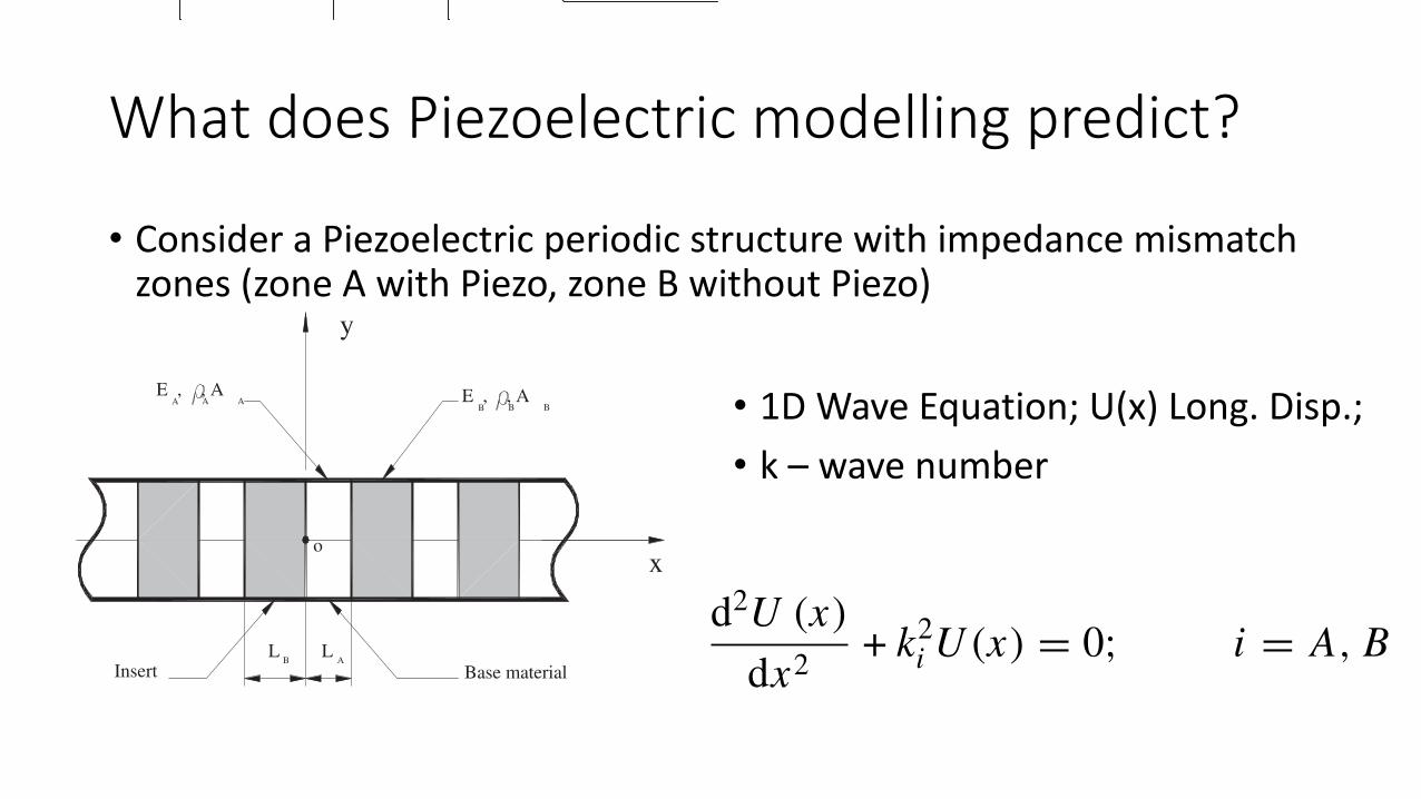
• ConsideraPiezoelectricperiodicstructurewithimpedancemismatchzones(zoneAwithPiezo,zoneBwithoutPiezo)O Thorp et al

LInsert

E , , A

ox

Base materialL

E , , A

y

AB

A AB B

B A

Figure 1. Periodic structure with impedance mismatch zones.

of the SMA inserts are used to modify the ability of the periodicrod to transmit waves. In [12], particular emphasis is placedon studying the characteristics of the rod when aperiodicity isintroduced in order to localize the vibration near the excitationsources. The study is guided by the early findings on thelocalization phenomena in disordered structures in the field ofsolid-state physics [13] and by the extensive wealth of availableliterature in structural dynamics (e.g. [14, 15]).

In this study, a radically different approach is adoptedwhereby the capabilities of classical periodic structuresto attenuate the propagation of waves are enhancedby augmenting these structures with the well-knownenergy dissipation characteristics of shunted piezoelectricmaterials [16–18].

Emphasis is placed in this paper on developing thefundamentals that govern the dynamics of wave propagationin rods with periodically placed shunted piezoelectric patches.The effect of uniform tuning of the shunting parameters ofall the patches on the location and the width of the pass andstop band characteristics will be investigated. Furthermore,the potential of introducing intentional aperiodicity byrandomizing the shunting parameters of the patches on thelocalization of vibration will also be demonstrated.

The paper is organized into five sections. In thefirst section a brief introduction is given. Section 2presents the fundamentals of wave propagation in one-dimensional systems using the transfer matrix approach aswell as the mathematical model for shunted piezoelectricmaterials. Section 3 investigates the performance of theconsidered periodic rod in terms of propagation constants,force transmission and deformed shape. The effect of disorderon the wave propagation characteristics is studied in section 4.The localization factor and the vibration localization areevaluated for rods with different levels of disorder subjectedto different excitation frequencies. Section 5 summarizesthe results obtained and provides some recommendations forfuture work.

2. Wave propagation in rods with periodic shuntedpiezoelectric patches

2.1. Transfer matrix formulation

The longitudinal wave propagation, at frequency ω, in aperiodic rod as shown in figure 1 is described by the solutionof the one-dimensional wave equation

d2U (x)

dx2+ k2

i U(x) = 0; i = A, B (1)

where U(x) is the longitudinal displacement of the rod atlocation x. Also, ρi and Ei denote respectively the density andYoung’s modulus of the ith layer and ki = ω

√ρi/Ei = ω/ci

is the corresponding wavenumber, with ci =√

Ei/ρi denotingthe wave speed.

The state vector Ykr at the right end (x = LB) of the kthcell of the periodic structure can be defined as follows:

Ykr =!

Ukr

...Nkr

"T (2)

where Nkr denotes the longitudinal force. The state vector atthe right end of an elementary cell is related to the state vectorat the left end as

Ykr = TkYkl . (3)

In equation (3), Tk is the cell transfer matrix, which isgiven by

Tk = T(B)k T

(A)k (4)

where

T(i)k =

#

cos(kiLi)sin(kiLi )

ziω

−ziω sin(kiLi) cos(kiLi)

$

, i = A, B. (5)

Equation (5) is obtained by recasting the dynamic stiffnessmatrix of rods [2] in the above transfer matrix form. Inequation (5), zi is the impedance of the ith layer of a semi-infinite rod, defined as

zi = Ai

%

Eiρi i = A, B (6)

with zi = Ai, Ei and ρi denoting the cross-sectional area,Young’s modulus and density of the ith layer, respectively.

980

• 1DWaveEquation;U(x)Long.Disp.;• k– wavenumber

O Thorp et al

LInsert

E , , A

ox

Base materialL

E , , A

y

AB

A AB B

B A









d2U (x)

dx2+ k2

i U(x) = 0; i = A, B (1)


√ρi/Ei = ω/ci




Ykr =!

Ukr

...Nkr

"T (2)


Ykr = TkYkl . (3)


Tk = T(B)k T

(A)k (4)

where

T(i)k =

#

cos(kiLi)sin(kiLi )

ziω


$

, i = A, B. (5)


zi = Ai

%

Eiρi i = A, B (6)


980

Solutionofthewaveequation• StateVector

O Thorp et al

(a)

(b)

0 500 1000 1500 2000 2500 3000 3500 4000 4500 5000 0

0.2

0.4

0.6

0.8

1

1.2

1.4

Frequency [Hz]

0 500 1000 1500 2000 2500 3000 3500 4000 4500 5000 0

0.1

0.2

0.3

0.4

0.5

0.6

0.7

0.8

0.9

1

Frequency [Hz]

η DSU E/E

Figure 2. Effective material properties of a piezoeletric patch withresistive (a) and inductive/resistive (b) shunting.

where ESUjj (ω) is the storage modulus and η(ω) is the loss

factor of the shunted piezoelectric patch. The effects of thefrequency on the storage modulus, normalized to the storagemodulus of the open circuit, and on the loss factor are shownin figure 2. The figure shows that the shunting circuit canmodify the dynamic properties gradually as in the case ofresistive shunting (figure 2(a)) or sharply as in the case ofresistive/inductive shunting (figure 2(b)). The location of thefrequency band, where the modifications can occur graduallyor sharply, can be selected by proper tuning of the shuntingcircuit parameters. The values of the tuning frequencies fordifferent shunting circuits are given in [16] and are summarizedin table 1.

Table 1. Optimal shunting parameters.

Shunting circuit Resistive Resistive/inductive

Tuning frequency ωtun =

!

1 − k2ij

R · CSpi

ωtun = 1!

L · CSpi

ZSU

Piezoelectric patch

ZSU

Base structure Shunting impedance

ZSU ZSU

Figure 3. Periodic rod with periodic shunted piezoeletric patches.

Piezo patch Base rod

Exciter 72.4 72.4

72.4

Figure 4. Rod with four shunted piezoelectric patches.

2.4. Mechanical impedance of rod with shunted piezoelectricpatch

The transfer matrix T (B) of the portion of the rod treated withthe piezoelectric patches (figure 4) can be calculated usingequation (5) such that the impedance of a composite rod zB isgiven by

zB ="

(ρAAA + ρPAP)#

EAAA + ESUjj AP

$

(19)

and

kB = ω

"

(ρAAA + ρPAP) /#

EAAA + ESUjj AP

$

(20)

where AA and AP denote, respectively, the cross sections of therod and of the piezoelectric patch, ρA and ρP are the densities ofthe rod and of the piezoelectric and EA is the Young’s modulusof the rod material.

The treatment of a portion of the rod produces a change ofimpedance due to the added stiffness of the piezoelectric and tothe additional stiffness corresponding to the shunting circuit.The latter is frequency dependent as suggested by figure 2and it can be modified around specified frequency bands bytuning the shunting circuit according to table 1. The change inimpedance generated by adding the piezoelectric patches canbe evaluated by defining a relative impedance ζ as

ζ = zB

zA(21)

where zA = AA√

EAρA is the impedance of the base rod andzB is the impedance of the treated portion of the rod, defined

982

O Thorp et al

(a)

(b)

0 500 1000 1500 2000 2500 3000 3500 4000 4500 5000 0

0.2

0.4

0.6

0.8

1

1.2

1.4

Frequency [Hz]

0 500 1000 1500 2000 2500 3000 3500 4000 4500 5000 0

0.1

0.2

0.3

0.4

0.5

0.6

0.7

0.8

0.9

1

Frequency [Hz]

η DSU E/E

Figure 2. Effective material properties of a piezoeletric patch withresistive (a) and inductive/resistive (b) shunting.

where ESUjj (ω) is the storage modulus and η(ω) is the loss

factor of the shunted piezoelectric patch. The effects of thefrequency on the storage modulus, normalized to the storagemodulus of the open circuit, and on the loss factor are shownin figure 2. The figure shows that the shunting circuit canmodify the dynamic properties gradually as in the case ofresistive shunting (figure 2(a)) or sharply as in the case ofresistive/inductive shunting (figure 2(b)). The location of thefrequency band, where the modifications can occur graduallyor sharply, can be selected by proper tuning of the shuntingcircuit parameters. The values of the tuning frequencies fordifferent shunting circuits are given in [16] and are summarizedin table 1.

Table 1. Optimal shunting parameters.

Shunting circuit Resistive Resistive/inductive

Tuning frequency ωtun =

!

1 − k2ij

R · CSpi

ωtun = 1!

L · CSpi

ZSU

Piezoelectric patch

ZSU

Base structure Shunting impedance

ZSU ZSU

Figure 3. Periodic rod with periodic shunted piezoeletric patches.

Piezo patch Base rod

Exciter 72.4 72.4

72.4

Figure 4. Rod with four shunted piezoelectric patches.

2.4. Mechanical impedance of rod with shunted piezoelectricpatch

The transfer matrix T (B) of the portion of the rod treated withthe piezoelectric patches (figure 4) can be calculated usingequation (5) such that the impedance of a composite rod zB isgiven by

zB ="

(ρAAA + ρPAP)#

EAAA + ESUjj AP

$

(19)

and

kB = ω

"

(ρAAA + ρPAP) /#

EAAA + ESUjj AP

$

(20)

where AA and AP denote, respectively, the cross sections of therod and of the piezoelectric patch, ρA and ρP are the densities ofthe rod and of the piezoelectric and EA is the Young’s modulusof the rod material.

The treatment of a portion of the rod produces a change ofimpedance due to the added stiffness of the piezoelectric and tothe additional stiffness corresponding to the shunting circuit.The latter is frequency dependent as suggested by figure 2and it can be modified around specified frequency bands bytuning the shunting circuit according to table 1. The change inimpedance generated by adding the piezoelectric patches canbe evaluated by defining a relative impedance ζ as

ζ = zB

zA(21)

where zA = AA√

EAρA is the impedance of the base rod andzB is the impedance of the treated portion of the rod, defined

982

• Impedance

• WaveConstant

O Thorp et al

LInsert

E , , A

ox

Base materialL

E , , A

y

AB

A AB B

B A









d2U (x)

dx2+ k2

i U(x) = 0; i = A, B (1)


√ρi/Ei = ω/ci




Ykr =!

Ukr

...Nkr

"T (2)


Ykr = TkYkl . (3)


Tk = T(B)k T

(A)k (4)

where

T(i)k =

#

cos(kiLi)sin(kiLi )

ziω


$

, i = A, B. (5)


zi = Ai

%

Eiρi i = A, B (6)


980

O Thorp et al

LInsert

E , , A

ox

Base materialL

E , , A

y

AB

A AB B

B A









d2U (x)

dx2+ k2

i U(x) = 0; i = A, B (1)


√ρi/Ei = ω/ci




Ykr =!

Ukr

...Nkr

"T (2)


Ykr = TkYkl . (3)


Tk = T(B)k T

(A)k (4)

where

T(i)k =

#

cos(kiLi)sin(kiLi )

ziω


$

, i = A, B. (5)


zi = Ai

%

Eiρi i = A, B (6)


980

O Thorp et al

LInsert

E , , A

ox

Base materialL

E , , A

y

AB

A AB B

B A









d2U (x)

dx2+ k2

i U(x) = 0; i = A, B (1)


√ρi/Ei = ω/ci




Ykr =!

Ukr

...Nkr

"T (2)


Ykr = TkYkl . (3)


Tk = T(B)k T

(A)k (4)

where

T(i)k =

#

cos(kiLi)sin(kiLi )

ziω


$

, i = A, B. (5)


zi = Ai

%

Eiρi i = A, B (6)


980

• CellTransferMatrix

Note𝐸>>?@ iscomplexandhence,theEigenvaluesoftheTransferMatrixwillbecomplex,wheretherealpartindicateswaveattenuationandimaginarypartindicateswavepropagation

PiezoelectricmodellingpredictsStopBandsandPropagation• ThePlotofRealandImaginarypartsoftheEigenvaluewithfrequencyshowsexistenceofpropagationandstopbands.

Attenuation and localization of wave propagation in rods with periodic shunted piezoelectric patches

(a)

(b)

Rel

ativ

e Im

peda

nce

ζ

Frequency [Hz]

R=10 Ω, L=0R= Ω, L=0Short Circuit

0 0.2 0.4 0.6 0.8 1 1.2 1.4 1.6 1.8 2

x 10 4

0

0.1

0.2

0.3

0.4

0 0.2 0.4 0.6 0.8 1 1.2 1.4 1.6 1.8 2

x 10 4

0

1

2

3

4

Rea

l(µ )

Im

ag(µ

)

Frequency [Hz]

0 0.2 0.4 0.6 0.8 1 1.2 1.4 1.6 1.8 2

x 104

1.3

1.31

1.32

1.33

1.34

1.35

1.36

1.37

1.38

1.39

1.4

100

Figure 5. Propagation constants (a) and relative impedance (b) forresistive shunting.

in equation (19). Substituting the expressions for zA and zB ,the relative impedance ζ can be rewritten as

ς =

!

"

"

#

$

1 +ρPAP

ρAAA

%

&

1 +ESU

jj AP

EAAA

'

. (22)

2.5. Response to harmonic excitation

The transfer matrix approach presented in section 2.1 can beused to evaluate the amplitude of the response along the rodfor harmonic excitation.

The state vectors at the beginning and the end of thestructure are related by the system transfer matrix T :

Yn = T Y0 or(

Un

Nn

)

=*

T11 T12

T21 T22

+(

U0

N0

)

(23)

where subscripts ‘0’ and ‘n’ denote, respectively, the statevectors at the beginning and at the end of the periodic structure.For a periodic system, the transfer matrix is the same for everycell and therefore

T = T nk (24)

where n is the number of cells and Tk is the transfer matrix ofone cell.

(a)

(b)

Frequency [Hz]

Rel

ativ

e Im

peda

nce

ζ

Frequency [Hz]

Rea

l(µ )

Im

ag(µ

)

0 0.2 0.4 0.6 0.8 1 1.2 1.4 1.6 1.8 2 x 10 4

0 0.1 0.2 0.3 0.4 0.5

0 0.2 0.4 0.6 0.8 1 1.2 1.4 1.6 1.8 2 x 10 4

0 1 2 3 4

0 0.2 0.4 0.6 0.8 1 1.2 1.4 1.6 1.8 2 x 10 4

1.25

1.3

1.35

1.4

1.45

1.5

Figure 6. Propagation constants (a) and relative impedance (b) forresistive/inductive shunting. (a) R = 10 $, L = 0.84 × 10−3 H(- - - -); R = 10 $, L = 0.29 × 10−3 H (— · —); R = 10 $,L = 0.14 × 10−3 H (——); and the thin solid curve represents theshort circuit case.

Equation (23) can be expanded as follows:

andUn = T11U0 + T12N0

Nn = T21U0 + T22N0(25)

where U0, Un and N0, Nn are the amplitudes of the longitudinaldisplacements and forces at the beginning and at the end of therod, respectively.

The boundary conditions for a rod fixed at node ‘n’ andexcited at its free end ‘0’ by a harmonic longitudinal force canbe expressed as follows:

U0 = 0

Un = 0and

N0 = f0

Nn = 0(26)

where f0 is the amplitude of the applied excitation.According to equations (25), the displacement U0 at the

free end can be obtained from the first of equations (26):

U0 = −T −111 T12N0. (27)

983

O Thorp et al

LInsert

E , , A

ox

Base materialL

E , , A

y

AB

A AB B

B A









d2U (x)

dx2+ k2

i U(x) = 0; i = A, B (1)


√ρi/Ei = ω/ci




Ykr =!

Ukr

...Nkr

"T (2)


Ykr = TkYkl . (3)


Tk = T(B)k T

(A)k (4)

where

T(i)k =

#

cos(kiLi)sin(kiLi )

ziω


$

, i = A, B. (5)


zi = Ai

%

Eiρi i = A, B (6)


980

EAPsarebroadlyclassifiedintotwogroups– ElectronicEAPandIonicEAPElectronicEAP(EEAP) IonicEAP(IEAP)

DielectricEAP IonicPolymerGels(IPG)

ElectrostrictivePaper IonicPolymerMetalComposite(IPMC)Nafion &Flemion

FerroelectricPolymers ConductingPolymersPpy,PA

LiquidCrystalElastomer CarbonNanotubes(CNT)

“InelectronicEAPs,theelectricfieldappliescoulombattractiveforcestotheelectrodes.Thiscausesthechangeinsizeandshapeduetocompressiveforces.WithionicEAPs,themobilityanddiffusionofionschangestheshape.”

AreBilayerlipidmembranes(BLM)piezoelectricorelectro-active?• ResponseoftheNeuronstoNerveimpulsesisgenerallyinthemillisecondregionwhichsupportstheexistenceofpiezoelectricity.• However,theionicmotionismorefeasibleduetothemovementofNaandKions.

Or:AretheyElectro-thermo-mechanicalSystem?

2

be considered as a SmA* phase (Sm stands for smectic, which indicates layered structure; A means that the average molecular orientation (director) is normal to the layers, and * indicates that the constituent molecules are chiral). Such a phase has D∞ symmetry and therefore must be piezoelectric, because by tilting the molecules, induced by shear and/or layer compression, one induces a SmC* phase, which has polar C2 symmetry with the polar axis normal to the tilt plane.13

In this paper we concentrate on this piezoelectric property of bare lipid bilayers. We show that piezoelectricity of lipid bilayers might explain previously observed ferroelectric-like behavior14 of ion channels and may have consequences in various sensory mechanisms. As op-posed to the flexoelectric polarization, here the tilt induced polarization occurs within the insulat-ing chains of the bilayers and therefore cannot be screened out by free ions of the surrounding aqueous plasma. We studied these properties using a hydrated phospholipid extract of egg yolk from Avanti Inc., which forms a stable SmA* liquid crystal phase in bulk over a wide tempera-ture range including the room temperature.15 The pictorial representation of the physical mecha-nism of the piezoelectricity, and the molecular structure of the major phospholipid component of the mixture, L-α-Phosphatidylcholine, are illustrated in Figure 1.

Figure 1: Illustration of the molecular structure of phospholipid L-α-Phosphatidylcholine and of the piezoelectricity of a lipid bilayer. A tilt of the average molecular orientation (director) with respect to the layer normal, induced by mechanical shear and/or layer compression, leads to a SmC* configuration with polarization normal to the tilt (shear) plane.

We assert that the lipid bilayers of cell membranes have this local SmA* structure, sug-gesting that real biological membranes are piezoelectric and electric charges are generated along the membrane when the lipids become tilted due to mechanical stimuli. Furthermore, we believe that cell membrane piezoelectricity may have numerous applications in biological processes. For example, it could explain communication between proteins embedded in cell membranes, or al-low the conversion of external stimuli to electric signals within sensory proteins. One specific sensory mechanism that we suspect might be possible is magneto-reception, where animals use ferromagnetic particles to sense local changes in magnetic fields. Homing pigeons, as well as many other animals have the ability to travel long distances without landmarks and arrive at their destinations with very high accuracy.16 For example, salmon, having spent most of their life in

electronic-Liquid Crystal Communications April 10, 2007

http://www.e-lc.org/docs/2007_04_09_12_01_56

Thepictorialrepresentationofthephysicalmechanismofthepiezoelectricity,andthemolecularstructureofoneofthemajorphospholipidcomponentsofthemixture,L-α-Phosphatidylcholine,areillustrated.TheexperimentsclaimedtoverifyPiezoelectricnatureoftheliquidcrystal.

7

0

5

10

15

20

0 20 40 60 80 100

Shear aligned lipid+ferrofluidNot Sheared lipid+ferrofluidpure phospholipidempty cellferrofluid

Magnetic Field (Gauss)

Cur

rent

(pA

)

a b

Figure 6 : Electric current induced by 1.1Hz periodic magnetic field that causes reorientation of the director in the plane along the electrode wires. (a): Magnetic field dependence of the phos-pholipid – 0.5wt% ferrofluid mixtures in different alignments and of the control groups; (b): The temperature dependence of the current of the aligned mixture at 100G. To summarize, we have unambiguously demonstrated the piezoelectricity of bare lipid bi-layers. In addition this current appears within the structured part of the membrane, so they are normally not screened out by ions surrounding the membrane; therefore the lateral background noise level is lower as indeed found on the control phospholipid samples. We have also clearly shown the effect of magnetic particles on electric responses of bilayer systems, supporting the magnetite model for magneto-reception. Although our magnetically induced signals are small, we emphasize that in real receptor cells the deformations are much larger than in the experiments we have used, so they may result in stronger localized signals.

Accordingly, we are convinced that study of the piezoelectric signals within the cell membrane is worthwhile and may shed light on a number of biophysical processes involving signaling within the cell membranes.

Acknowledgement: The work was partially supported by NSF DMS 0456221. We thank to Professor Philip

Westerman for helpful discussions, Dr. G. Liao, T. Heatdrech and C. Braganza for their in-volvement in early stages of the experiments.

0

5

10

15

20

60 80 100 120Temperature ( oC)

Cur

rent

(pA

)



4

For the piezoelectric measurements (Figure 2a) the liquid crystal material is sandwiched

between two glass plates (2 and 2’) that are firmly fixed to temperature stabilized heaters (1 and 1’). A pair of piezoelectric plates (5,6), sensitive to forces in the lateral directions, is attached to the bottom of the lower heated plate, which is connected to a rigid frame (8) via three layers of piezo sensors (5,6,7) sensitive in orthogonal directions. The frame also holds a piezoelectric ac-tuator (9) ((PSt 500/10/5 from Piezomechanik GmbH), which can shift the top plate with maxi-mum amplitude of 5μm. The actuator is driven by a high voltage amplifier (LE 430/015 from Piezomechanik GmbH). The motion of the top plate is monitored by a piezoelectric accelerome-ter (BK 4375 from Bruel & Kjaer, sensitivity 0.1mm/s2). The sample holder is placed in a polar-izing microscope (10), which enables textural observations of the sample during the measure-ments. One can make controlled periodic shear deformations of a given frequency and detect the induced corresponding current using a lock-in amplifier (7265 DSP from PerkinElmer). As shown in Figure 3a, an important feature of the vibration created by this setup is that it is along the y direction only at frequencies below 200 Hz, and at higher frequencies there are num-ber of resonances where the vertical vibration becomes generated with basically similar ampli-tudes.

0

0.4

0.8

1.2

0 200 400 600 800 1000

verticalhorizontal

Frequency (Hz)

Dis

palc

emen

t (μm

)

0

100

200

300

400

0 200 400 600 800 1000

71oC62oC53oC23oC

Frequency (Hz)

P (n

C/c

m2 )

a b

Figure 3: (a): Frequency dependences of the amplitudes of the vibrations of the top plate in ver-tical (Δx) and horizontal (Δy) displacements. (b): The frequency dependence of the induced electric polarization P calculated from the piezo-current I as /( )P I A ω= ⋅ , where A~0.6mm2 is the area of the electrode and ω is the angular frequency. Comparing Figure 3a and b, one can see that the peak positions measured in the vibration of the top plate and of the induced currents correspond to each other (the correspondence is more evi-dent at low frequencies). The frequency dependence of the induced polarization (see Figure 3/b) shows that the response is decreasing toward lower temperatures as the material becomes stiffer. We note that the modulus of the piezo actuator is much larger than of the lipid even at room temperature and the measured displacement of the top plate is basically temperature independent. The amplitude of the current measured at different runs increases after the initial frequency scans. Simultaneous textural observations (see Figure 4) revealed improving homeotropic alignment during the vibration of the upper plate.



Jakli etal:ElectronicLiquidCrystalCommunications

NewworksintheHorizonARTICLEReceived 17 Oct 2014 | Accepted 19 Feb 2015 | Published 30 Mar 2015

Mechanical surface waves accompany actionpotential propagationAhmed El Hady1,2,* & Benjamin B. Machta3,4,*

Many diverse studies have shown that a mechanical displacement of the axonal membrane

accompanies the electrical pulse defining the action potential (AP). We present a model for

these mechanical displacements as arising from the driving of surface wave modes in which

potential energy is stored in elastic properties of the neuronal membrane and cytoskeleton

while kinetic energy is carried by the axoplasmic fluid. In our model, these surface waves are

driven by the travelling wave of electrical depolarization characterizing the AP, altering

compressive electrostatic forces across the membrane. This driving leads to co-propagating

mechanical displacements, which we term Action Waves (AWs). Our model allows us to

estimate the shape of the AW that accompanies any travelling wave of voltage, making

predictions that are in agreement with results from several experimental systems. Our model

can serve as a framework for understanding the physical origins and possible functional roles

of these AWs.

DOI: 10.1038/ncomms7697

1 Princeton Neuroscience Institute, Princeton University, Princeton, New Jersey 08544, USA. 2 Howard Hughes Medical Institute, Princeton University,Princeton, New Jersey 08544, USA. 3 Lewis-Sigler Institute, Princeton University, Princeton, New Jersey 08544, USA. 4 Department of Physics, PrincetonUniversity, Princeton, New Jersey 08544, USA. * These authors contributed equally to this work. Correspondence and requests for materials should beaddressed to A.E.H. (email: [email protected]) or to B.B.M. (email: [email protected]).

NATURE COMMUNICATIONS | 6:6697 | DOI: 10.1038/ncomms7697 | www.nature.com/naturecommunications 1

& 2015 Macmillan Publishers Limited. All rights reserved.

References• A.L.Hodgkin,A.F.Huxley,Aquantitativedescriptionofmembranecurrentanditsapplicationtoconductionandexcitationinnerve,J.Physiol.117(1952)500–544.

• I.Tasaki,K.Kusano,M.Byrne,Rapidmechanicalandthermalchangesinthegarfisholfactorynerveassociatedwithapropagatedimpulse,Biophys.J.55(1989)1033–1040.

• I.Tasaki,M.Byrne,Volumeexpansionofnonmyelinated nervefibersduringimpulseconduction,Biophys.J.57(1990)633–635.

• T.Heimburg,A.D.Jackson,Onsolitonpropagationinbiomembranes andnerves,Proc.Natl.Acad.Sci.U.S.A.102(2005)9790–9795.

• M.Argentina,P.Coullet,V.Krinsky,Head-oncollisionsofwavesinanexcitableFitzHugh-Nagumosystem:atransitionfromwaveannihilationtoclassicalwavebehav- ior,J.Theor.Biol.205(2000)47–52.

• R.Appali,S.Petersen,U.vanRienen,AcomparisonofHodgkin-Huxleyandsolitonneuraltheories,Adv.RadioSci.8(2010)75–79.

• OThorp,MRuzzene2andABaz,Attenuationandlocalizationofwavepropagationinrodswithperiodicshuntedpiezoelectricpatches,(2001)SmartMater.Struct.10979

on some electro-mechanical aspects of neuron model · discovery of nerve impulse flow from a squid...

Documents