on solutions to the yang-baxter equation related to sl(n)
TRANSCRIPT

On solutions to the Yang-Baxterequation related to sl(n)
Gary Bosnjak
A thesis submitted for the degree of
Doctor of Philosophy
September 2017

c© Gary Bosnjak 2017

I declare that the work contained in this thesis is my own original research, obtainedin collaboration with my supervisor Dr. Vladimir Mangazeev at the Australian
National University, Canberra. All material taken from other sources is referenced andacknowledged as such. I also declare that none of the material contained in this thesis
has been submitted for another degree at this or another university.
Gary Bosnjak
30 September 2017


Acknowledgments
I would first like to acknowledge and thank my supervisors Vladimir Bazhanov andVladimir Mangazeev for taking me on as a PhD student. I am grateful to have hadthe opportunity to study under some of the foremost experts in quantum integrabil-ity, and no doubt they have had an enormous influence on my mathematical interests;introducing me to all kinds of new mathematics and physics where I think there arevery many exciting discoveries to be made. Especially Mangazeev who I have workedclosely with in the development of the results in this thesis, and from which we havewritten (and still need to write!) papers together. I am also thankful for all the wisdomand hard lessons I have received in trying to establish myself as a researcher. The per-sonal growth I have undergone these past few years has been extraordinary.
Ofcourse I would like to thank my family, so thanks Mum, Dad, Daniel and Andrew. Isometimes feel like I don’t deserve the support I get from you people, but it seems thatthe love really is unconditional! All of the frequent visits and accommodation are verymuch appreciated. They say you can’t choose your family but I wouldn’t have it anyother way! I just hope the feeling is mutual because you might have to put up with memore often now.
Obviously I met a lot of interesting people during my time as a PhD student. There aremany names but I want to especially acknowledge a few other research students whohad an impact on me as an intellectual and a friend. Brendan Wilson my officematewho taught me a lot of physics, programming and got me into bike touring. TitouanSerandour, Song Cheng, Michael Canagasabey whom I had lots of fun discussions withabout maths and everything else, and Gleb Kotousov, who is an interesting character.
Finally I want to acknowledge the Australian National University, who provided mewith the funding that enabled this opportunity. It is a lovely research environment andthe staff have been nothing but wonderful to me. I am a little reluctant to leave to behonest. I hope I can come back!
v


Abstract
In this thesis the problem of constructing solutions to the Yang-Baxter equation is con-sidered. Such solutions are known as R-matrices and we study a certain class of theserelated to the quantum group Uq(sln). Using a variety of unrelated methods the ma-trix elements for different representations of the quantum group are constructed. Inthe process the structure of the solutions and their symmetries are detailed including arealisation of the R-matrix as a "composite object".
Among the new results obtained is a formula for the elements of the general Uq(sln)
R-matrix for symmetric tensor representations with arbitrary weights in terms of mul-tivariable q-hypergeometric series. This formula is shown to be factorised by moreelementary R-matrices without the difference property. An explicit formula for the fac-tors in terms of simple products is derived from the general formula by evaluating theR-matrix at special values of the spectral parameter. Using this factorisation a simpleproof that the newly obtained R-matrix can be stochastic is given. Symmetries of theR-matrix generate identities of hypergeometric series which may be unknown.
This new factorised representation of the R-matrix is compared with other construc-tions developed in the literature. It is shown that there is agreement up to simpletransforms between all the R-matrices considered, thereby linking different approachesto solving Yang-Baxter equation. In the process comparisons between different formu-lae for the matrix elements are made which reveal that the 3D approach based on a newsolution to the tetrahedron equation is the most efficient construction for this class ofR-matrices. In some cases comparisons can only be made in the rational limit q → 1and using the newly obtained trigonometric R-matrix a quantum deformation of theirconstruction is given. These deformations are used to discover new structure of thetrigonometric R-matrix, such as a new L-operator factorisation in the rank 1 case aswell some new formulae for the generating function of the operator action.
Some progress is made towards a more general formula for matrix elements in thecase of arbitrary highest weight representations of sln. Using a factorisation approachby Derkachov et al. explicit formulae for the elements of the factors in the case n = 3 is
vii

viii
presented. These factors are shown to be related to the new trigonometric factorisationpresented in this thesis.
Finally, the stochastic R-matrix is linked to recent developments in near-equilibriumstochastic systems of interacting particles of KPZ universality class. The factorisation ofthe matrix is shown to be equivalent to a "convolution" of the probability function de-scribing these models. A generalisation of this probability function in the case of sl(3)is proposed which contains an extra parameter and seems to satisfy the sum-to-unityrule.

Contents
Acknowledgments v
Abstract vii
1 Thesis Overview 1
2 Yang-Baxter Integrability 7
2.1 Integrable systems . . . . . . . . . . . . . . . . . . . . . . . . . . . . . . . . 7
2.2 Statistical mechanics . . . . . . . . . . . . . . . . . . . . . . . . . . . . . . . 10
2.2.1 The six-vertex model . . . . . . . . . . . . . . . . . . . . . . . . . . . 13
2.2.2 The transfer matrix . . . . . . . . . . . . . . . . . . . . . . . . . . . . 14
2.3 Yang-Baxter integrability . . . . . . . . . . . . . . . . . . . . . . . . . . . . . 17
2.3.1 Bethe ansatz . . . . . . . . . . . . . . . . . . . . . . . . . . . . . . . . 17
2.3.2 Commuting transfer matrices . . . . . . . . . . . . . . . . . . . . . . 19
2.4 Quantum groups . . . . . . . . . . . . . . . . . . . . . . . . . . . . . . . . . 24
2.4.1 Quantum inverse scattering method . . . . . . . . . . . . . . . . . . 25
2.4.2 The quantum group Uq(sln) . . . . . . . . . . . . . . . . . . . . . . 27
3 A 3D Integrable Model 39
3.1 The tetrahedron equation . . . . . . . . . . . . . . . . . . . . . . . . . . . . 40
3.2 A solution with positive Boltzmann weights . . . . . . . . . . . . . . . . . 42
ix

x Contents
3.2.1 q-oscillator algebra and Fock space representations . . . . . . . . . 43
3.2.2 Functional Tetrahedron equation . . . . . . . . . . . . . . . . . . . . 44
3.3 n-layer projection . . . . . . . . . . . . . . . . . . . . . . . . . . . . . . . . . 47
3.4 Symmetries and special cases . . . . . . . . . . . . . . . . . . . . . . . . . . 55
3.5 Reductions and factorization . . . . . . . . . . . . . . . . . . . . . . . . . . 56
3.6 Comparison with other results . . . . . . . . . . . . . . . . . . . . . . . . . 58
3.7 Rational limit . . . . . . . . . . . . . . . . . . . . . . . . . . . . . . . . . . . 62
3.7.1 Rational L-operator . . . . . . . . . . . . . . . . . . . . . . . . . . . . 64
3.7.2 Factorization . . . . . . . . . . . . . . . . . . . . . . . . . . . . . . . 66
3.8 A polynomial representation . . . . . . . . . . . . . . . . . . . . . . . . . . 67
4 Spectral decomposition 71
4.1 The Jimbo equations . . . . . . . . . . . . . . . . . . . . . . . . . . . . . . . 71
4.2 The case Uq(sl2) . . . . . . . . . . . . . . . . . . . . . . . . . . . . . . . . . . 74
4.2.1 Quantum Clebsch-Gordan coefficients . . . . . . . . . . . . . . . . . 74
4.2.2 An explicit formula . . . . . . . . . . . . . . . . . . . . . . . . . . . . 77
4.2.3 Transformation to a single sum . . . . . . . . . . . . . . . . . . . . . 78
4.2.4 Discussion . . . . . . . . . . . . . . . . . . . . . . . . . . . . . . . . . 80
5 R-matrix factorisation by Q-operators 83
5.1 Factorized ansatz . . . . . . . . . . . . . . . . . . . . . . . . . . . . . . . . . 84
5.2 Principal series representations of SL(n, C) . . . . . . . . . . . . . . . . . . 86
5.3 Factorised form and properties . . . . . . . . . . . . . . . . . . . . . . . . . 90
5.4 Operator kernel and hermitian form . . . . . . . . . . . . . . . . . . . . . . 91

Contents xi
5.5 Construction for sl2 . . . . . . . . . . . . . . . . . . . . . . . . . . . . . . . . 93
5.5.1 Factor Identities . . . . . . . . . . . . . . . . . . . . . . . . . . . . . . 97
5.5.2 Discussion . . . . . . . . . . . . . . . . . . . . . . . . . . . . . . . . . 101
5.6 Construction for sl3 . . . . . . . . . . . . . . . . . . . . . . . . . . . . . . . . 102
5.6.1 The factor R(1)(λ) . . . . . . . . . . . . . . . . . . . . . . . . . . . . 109
5.6.2 The factor R(2)(λ) . . . . . . . . . . . . . . . . . . . . . . . . . . . . 110
5.6.3 The factor R(3)(λ) . . . . . . . . . . . . . . . . . . . . . . . . . . . . 112
5.6.4 Symmetric tensor representations . . . . . . . . . . . . . . . . . . . 113
5.6.5 Discussion . . . . . . . . . . . . . . . . . . . . . . . . . . . . . . . . . 118
6 L-operator factorisation 121
6.1 Factorization formula for the rational R-matrix . . . . . . . . . . . . . . . . 123
6.2 The trigonometric R-matrix . . . . . . . . . . . . . . . . . . . . . . . . . . . 126
6.3 A trigonometric factorization . . . . . . . . . . . . . . . . . . . . . . . . . . 128
6.4 An alternative derivation . . . . . . . . . . . . . . . . . . . . . . . . . . . . 134
6.4.1 q-deformation . . . . . . . . . . . . . . . . . . . . . . . . . . . . . . . 135
7 SU(2)-invariance and coherent state action 139
7.0.1 Transformation to a single sum . . . . . . . . . . . . . . . . . . . . . 143
7.0.2 q-deformation . . . . . . . . . . . . . . . . . . . . . . . . . . . . . . . 144
7.1 Generating function for q-action . . . . . . . . . . . . . . . . . . . . . . . . 146
8 A stochastic R-matrix 149
8.0.1 Symmetric tensor representations of Uq(sln) . . . . . . . . . . . . . 150
8.0.2 Towards an arbitrary highest weight generalisation . . . . . . . . . 154

xii Contents
9 Conclusion 157
9.1 Future Work . . . . . . . . . . . . . . . . . . . . . . . . . . . . . . . . . . . . 161
A Hypergeometric Series 165
A.1 Definitions . . . . . . . . . . . . . . . . . . . . . . . . . . . . . . . . . . . . . 165
A.2 Identities . . . . . . . . . . . . . . . . . . . . . . . . . . . . . . . . . . . . . . 166
A.2.1 Chapter 5 identities . . . . . . . . . . . . . . . . . . . . . . . . . . . 168
A.2.2 Chapter 6 identities . . . . . . . . . . . . . . . . . . . . . . . . . . . 169
A.2.3 Chapter 7 identities . . . . . . . . . . . . . . . . . . . . . . . . . . . 169
B Basic Hypergeometric Series 171
B.1 Definitions . . . . . . . . . . . . . . . . . . . . . . . . . . . . . . . . . . . . . 171
B.2 Identities . . . . . . . . . . . . . . . . . . . . . . . . . . . . . . . . . . . . . . 172
B.2.1 Chapter 4 identities . . . . . . . . . . . . . . . . . . . . . . . . . . . 174
B.2.2 Chapter 6 identities . . . . . . . . . . . . . . . . . . . . . . . . . . . 176
B.2.3 Chapter 7 identities . . . . . . . . . . . . . . . . . . . . . . . . . . . 177

List of Figures
2.1 Local site configurations allowed in the six-vertex model. . . . . . . . . . . 13
2.2 A possible configuration of a 4× 4 six-vertex model with periodic bound-ary conditions. . . . . . . . . . . . . . . . . . . . . . . . . . . . . . . . . . . . 14
2.3 Matrix elements for an operator R given by vertex configurations. . . . . 15
2.4 Graphical notation of the row-to-row transfer matrix T for M sites. . . . . 16
2.5 Matrix [S(λ, µ)] . . . . . . . . . . . . . . . . . . . . . . . . . . . . . . . . . . 21
2.6 Sufficiency condition for T (λ)T (µ) = T (µ)T (λ) . . . . . . . . . . . . . . 22
2.7 Yang-Baxter RLL-relation . . . . . . . . . . . . . . . . . . . . . . . . . . . . 26
3.1 Matrix elements for an operator R given by vertex configurations. . . . . 40
3.2 Tetrahedron equation in vertex form . . . . . . . . . . . . . . . . . . . . . . 41
3.3 Tetrahedron RLLL relation . . . . . . . . . . . . . . . . . . . . . . . . . . . . 42
3.4 n-layer projection of the 3-dimensional model . . . . . . . . . . . . . . . . 49
4.1 Tensor representation of Clebsch-Gordan coefficients . . . . . . . . . . . . 74
4.2 R-matrix representation as a sum of projection operators . . . . . . . . . . 76
4.3 Graphical representation of the R-matrix (4.2.19) . . . . . . . . . . . . . . . 81
xiii

xiv LIST OF FIGURES
Chapter 1
Thesis Overview
In this thesis we consider the problem of constructing solutions to the parametrisedquantum Yang-Baxter equation. That is, the linear operator equality
R12(λ1, λ2)R13(λ1, λ3)R23(λ2, λ3) = R23(λ2, λ3)R13(λ1, λ3)R12(λ1, λ2), (1.0.1)
acting on a tensor product of vector spaces V1 ⊗ V2 ⊗ V3. A solution R(λ) is a linear’R-operator/R-matrix’ acting on W⊗U such that Rij(λi, λj) acts as W = Vi, U = Vj andtrivially in the third space. It is also known as the triangle equation or 2-simplex equa-tion. Ever since the connection between this equation and the solvability of quantumsystems was realised, many approaches have been developed over the years as meansof constructing solutions and thereby examples of quantum systems that are solvable.The list of all approaches, as they are currently known are
1. Direct evaluation of the universal R-matrix [1; 2; 3]
2. Fusion procedure [4; 5; 6]
3. Projection of a 3D Integrable Model [7; 8; 9; 10]
4. Matrix factorization of the L-operator [11; 12]
5. Factorization of the R-matrix by Q-operators [13; 14]
6. Coherent state action on the holomorphic basis [15]
7. Spectral decomposition [16; 17; 18]
8. Direct solution to recurrence relations
Development of some approaches, such as 3, 4 and 5 are still ongoing. Others, suchas 1, 2, 6 and 7 have seen little progress in the last few decades and are perhaps (with
1

2 Thesis Overview
the exception of 6) more "mature" in their development. In most cases, the R-matrixis presented in an abstract "black box" form in which the finer features of the solutionare opaque. For example, up until now, matrix elements were only known explicitlyfor very few solutions whose structure is usually described by some low rank Lie alge-bra under a low dimensional fundamental or adjoint representation. We look to thesemethods in an attempt to construct matrix elements for higher rank Lie algebras forrepresentations acting on finite and infinite dimensional spaces. Every method we con-sider, offers in theory a way of doing this for at least some classes of solutions. Howeverin practice it is all too often an exhaustive computation and not feasible even with mod-ern computer algebra. Furthermore some approaches are instrinsically limited or notyet developed enough to construct many solutions. Therefore there are many solutionswhich we know to exist but we cannot write down their elements.
One of the major results of this thesis featured in chapter 3 is the construction of a mas-ter formula (3.3.24) giving the elements of every R-matrix related to Uq(sln) for symmet-ric tensor representations with arbitrary weights. The formula is presented in terms ofa multivariable basic hypergeometric series and is always a finite algebraic expressionwhich is very efficient to compute. This includes the case of complex weight parame-ters where the R-matrix is irreducible and acts on a tensor product infinite-dimensionalVerma modules. This work is a generalisation of the 3D projection approach used in[10] where the formula (3.8.3) was obtained in case n = 2. The formula is given in termsof a single variable basic hypergeometric series which matches the q-Racah polynomi-als [19] known in combinatorics. In chapter 4 we give another proof/derivation of thisformula using the representation theory of quantum groups directly.
We spend a great deal of time studying the structure of this formula, including itssymmetries, degenerations, and comparing it with other results obtained elsewhere inthe literature. These are some minor results contained in this thesis. Actually, the mostinteresting thing to come out of this study is a new factorization for this class of R-matrices in terms of two simpler R-matrices with two independent spectral parameters.We say they are simpler because they are obtained from the general R-matrix by evaluat-ing it at two special values of the spectral parameter. In these cases our formula (3.3.24)reduces to a simple binomial product with weight parameters entering the expressionalgebraically. Viewing these as spectral parameters it solves (1.0.1). Multiplying thesematrices back together with special arguments we can reconstruct the original R-matrixthereby factorising it. This is encapsulated in (3.5.6) and we consider it another majorresult of this thesis.

3
We are very excited by this factorisation, and we believe there is still much more tothe story regarding its reason for being and its applications. For example, the binomialproduct function determining matrix elements of the factors is actually the probabilitydistribution function Φ (8.0.4) first introduced in [20] as a higher rank generalisationof a four parameter family of integrable stochastic zero range processes [21; 22; 23; 24].Contained within this family are non-equilbrium systems of interacting particles be-longing to the Kardar-Parisi-Zhang universality class. It is clear that the Yang-Baxterequation is behind the integrability of these models and our factorisation implies thatthe matrix elements we have constructed are some kind of convolution of these proba-bility distribution functions. The explicit relation is given by (8.0.10) which we rewritehere in a more abstract form as
R(λ) = Φ ∗Φ, (1.0.2)
where R(λ) is a "twisted" version (8.0.1) of the R-matrix constructed in chapter 3. Thiselegant connection between the Uq(sln) R-matrix, typically known to describe a fam-ily of six-vertex-like models and 1D quantum spin-chain magnets, and these stochasticZRP models is unknown and therefore is another major result of this thesis. In addition,we use this result to give a simple proof that our R-matrix can be stochastic by showingthat its elements sum to unity down columns and are positive.
All of the results mentioned so far are obtained by using a solution (3.2.13) [9] to themore general tetrahedron/3-simplex equation and projecting it out in one direction. Weare interested in other ways R-matrices can be constructed, with the goal of unifyingthese approaches and constructing the elements of even more solutions to the Yang-Baxter equation which we expect also has interesting structure such as factorisationand stochasticity. We also want to see if it is possible to find a "better" formula than theone we have obtained and therefore find some interesting identities for hypergeometricseries. As we show in this thesis, each construction yields a very different presentationof the R-matrix. Even when two methods supposedly construct an identical matrix, theformula for the elements is often completely different. To illustrate, for the case of sl2 themethod of spectral decomposition in chapter 4 constructs a triple summation formula(4.2.9), while the factorisation methods of chapters 5 and 6 produce double summationand single summation (5.5.14) formulae respectively. Yet each formula produces (upto normalisation and simple transformations) the same R-matrices. In this thesis wespend much time showing how all these different presentations are actually the same,by using identities for hypergeometric series to transform and sum up all these differentformulae to the same result. So far we have completed this unification for sl2, where

4 Thesis Overview
we have derived the single summation formula (3.8.3) and its rational limit from allconstructions considered. From this exercise we conclude that this formula is simplestpresentation of sl2 related R-matrices. We do not believe it can be summed up furtheror transformed into an even simpler series. This unification is a main result of our work.
We believe this to be also true of our trigonometric R-matrix formula (3.3.24) and wehave made some progress towards reconstructing it with other approaches. Before weelaborate, let us be clear that the 3D and spectral decomposition methods are the onlyones considered in this thesis that construct trigonometric R-matrices. The methods inother chapter construct rational R-matrices which are a special case obtainable from thetrigonometric ones in the limit q → 1. We have successfully taken this limit in (3.3.24)to give another formula (3.7.4) for a family of sln related factorised rational R-matriceswhich we can directly compare to the constructions where the trigonometric version isunknown. Besides the aforementioned n = 2 case which we have unified in this thesis,we have succeeded in the case of n = 3 in section 5.6.4 for the rational R-matrix. Onething we have learnt is that the computational task involved in these alternative meth-ods is far greater than the 3D model projection method of chapter 3, and the resultantformulae are much more complicated. Hence our assertion that the 3D construction isthe most efficient for this particular class of R-matrices.
Given our unification and the unknown quantum deformation of the factorisation meth-ods of chapters 6, 5 and Sklyanin’s method in chapter 7 we use our trigonometric R-matrix to work out how they deform. We start from our Uq(sl2) R-matrix (3.8.3) andreverse the arguments made in the rational case and replace them with their quantumanalogues. We obtain the q-deformations of all the theory developed in what is essen-tially the q→ 1 limit and there are number of new results here. The main one is a newhigher spin Uq(sl2) L-operator/R-matrix factorisation (6.3.17) with explicit formulae forall the factors generalising the results in [12]. We also find that our factorisation (3.5.6)in the n = 2 case is actually the q-deformation of the Q-operator factorisation of chapter5 derived using a very different Lie group oriented approach [25; 14]. Therefore ourfactorisation is also a higher rank trigonometric generalisation of this construction.
In these rational R-matrix constructions we often have to consider a generating func-tion for the operator action to extract matrix elements. We also present a deformation ofthese functions for the action of the trigonometric R-matrix. For example, the R-matrixconstructed in chapter 7 has a generating function presented as a terminating 2F1 hy-pergeometric series. This presentation is particularly nice because its dependence onthe holomorphic basis of the underlying space is a function of only a single variable.

5
Besides showing that this R-matrix is exactly the same as that obtained from the 3Dapproach, we also found its quantum deformation and its generating function whichturns out to be a balanced and terminating 4φ3 basic hypergeometric series and it ap-pears that it no longer depends on a single variable. This is unfortunate, but the resultstill may be useful in integration involving quantum groups although this is a questionwe did not get around to investigating.
We are particularly interested in the construction of chapter 5 for a number of rea-sons. The first is because it is a factorisation in terms of objects similar to ones weobtained in (3.5.6), (3.7.18) and so the construction can probably be generalised in thisdirection. Secondly because it applies for all highest weight representations of sln andhence we could obtain a more general formula for a larger family of R-matrices. Weattempted this for the case of sl3 and mostly succeeded, where we constructed explicitformula for the elements of the three factors (5.6.15), (5.6.19), and (5.6.21) composingthe full R-matrix. The functions for their elements are already quite complicated andthe resultant function obtained by composing them together is even more complicated- containing 12 summations - so we do not write it down until we can find a way ofsumming it. Nevertheless the factors are interesting objects in their own right becausethey are a kind of R-matrix, satisfying identity (5.3.4d). This identity is essentially theYang-Baxter equation but with the extra complexity of the intertwining of representa-tions by each factor. This complexity can be removed at least in the n = 2 case bymaking the right variable substitution as in (5.5.17) where we showed it is the same asour factorisation. It is probable that the same can be done for the n = 3 factors we con-struct with this method. We also mention as another application that they are buildingblocks for constructing Q-operators as explained in [26; 27; 14]. This is not exploredany further in our thesis but it is something we would like to investigate in the future.
We also think there is an application of the chapter 5 construction to the aformentionedstochastic ZRP models. Given the similarity of that factorisation with ours (3.5.6) weask if they are also stochastic R-matrices. If they are then they must be something moregeneral because they are operators acting with more parameters. As we considered thesl3 construction we saw that one of the factors is described by a function that seems tosatisfy the sum-to-unity property. It has an extra parameter compared to the function(8.0.10) (for n = 3) describing stochastic R-matrices and it reduces to it when this extraparameter is set to 0. We cannot at this time give a proof of the sum to unity propertyor its positivity regimes, but propose this function as a possible generalisation whichmay be interpreted as a new collection of stochastic models - a conjecture.

6 Thesis Overview
The structure of this thesis is summarised as follows. Chapter 2 is a brief background ofYang-Baxter integrability. We present some history of the notion of integrability and themotivation for studying it as an enquiry into some of the most fundamental problemsin physics. We use this as a foundation to formally introduce the Yang-Baxter equation;how it appears and some of the discoveries made in attempts to solve it. The goal ofthis chapter is to provide some context for our work, and to explain where it fits in thebody of research on this topic. We also use it to introduce some of the notations, the-ory, and terminology used in this thesis and elsewhere, such as quantum groups andtheir representation theory. We will briefly mention some constructions that we did notconsider in this thesis, such as the universal R-matrix construction.
The rest of the thesis is divided into chapters based on each particular R-matrix con-struction we have considered. Chapter 3 is dedicated to the 3D model projection ap-proach where we use a solution of the tetrahedron equation to construct R-matrices.Chapter 4 is dedicated to the method of "spectral decomposition" where we use therepresentation theory of quantum groups to write down the R-matrix in terms of itseigenvalue decomposition on its subspaces which are described by Clebsch-Gordancoefficients. Chapter 5 is about a R-matrix factorisation in terms of more elementaryintertwining operators which are building blocks of Q-operators. Chapter 6 is anotherfactorisation approach that can be considered a continuation of chapter 5 when onetries to restrict that construction to the case of finite-dimensional R-matrices. Chapter 7is a construction of a SU(2) invariant R-matrix by considering its action on the coherentstate vector where it turns out to have nice transformation properties that can be ex-ploited. Chapter 8 is an investigation of the R-matrices considered as a stochastic objectwhere we prove its sum-to-unity property and link it back to the stochastic models. Theappendices are dedicated to hypergeometric series where we list all the definitions andidentities we use in writing down and transforming the formulae we derive in the maintext.
Finally, we would like to mention that some of this work has already been publishedin journals. The research on the 3D model approach in chapter 3 for Uq(sln) and itsstochastic interpretation in chapter 8 appears in [28]. The main results in chapters 6and 7 will appear in [29]. The results of other chapters may appear in later papers.
Chapter 2
Yang-Baxter Integrability
2.1 Integrable systems
In the discipline of physics one attempts to model the physical universe by buildinga complete, consistent theory from which predictions can be formulated and testedagainst experiment. In modern physics, popular theories such as the standard model arealmost completely mathematical, such that the core principles of the theory are writtenin the formal language of mathematics. This formalisation of physics is perhaps anongoing process since the time of Newton. His description of planetary motion as thesolution to some collection of mathematical equations birthed the fundamental physicscommonly known today as Classical Mechanics.
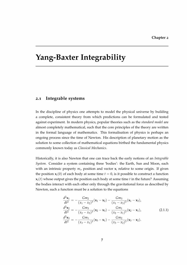
Historically, it is also Newton that one can trace back the early notions of an IntegrableSystem. Consider a system containing three ‘bodies’: the Earth, Sun and Moon, eachwith an intrinsic property mi, position and vector xi relative to some origin. If giventhe position xi(0) of each body at some time t = 0, is it possible to construct a functionxi(t) whose output gives the position each body at some time t in the future? Assumingthe bodies interact with each other only through the gravitational force as described byNewton, such a function must be a solution to the equations
d2x1
dt2 = − Gm2
(x1 − x2)3 (x1 − x2)−Gm3
(x1 − x3)3 (x1 − x3),
d2x2
dt2 = − Gm3
(x2 − x3)3 (x2 − x3)−Gm1
(x2 − x1)3 (x2 − x1), (2.1.1)
d2x3
dt2 = − Gm1
(x3 − x1)3 (x3 − x1)−Gm2
(x3 − x2)3 (x3 − x2).
7

8 Yang-Baxter Integrability
In mathematics (2.1.1) may be identified as a system of coupled, second-order linearordinary differential equations. One can imagine that a solution is of interest to mathe-maticians as a formal object unto itself. Yet it also practical applications,such as accurateprediction of future solar events.
In any case, it turns out a general solution satisfying any initial condition xi(0) doesnot have a ‘closed’ form. That is, the function xi(t) cannot be written down in terms ofelementary functions such as trignometric, exponential, logarithmic and algebraic func-tions. This was proven by Bruns and Poincare. Indeed, Newton himself had attempteda solution but failed. Sundman’s theorem gives an expression for xi(t) as an infinitepower series but this is not considered a closed-form solution. Furthermore, its conver-gence is so slow that computing a good approximation of the function is impractical.Perhaps it is worth noting that closed-form solutions have been found in some specialcases of the problem [30; 31; 32; 33].
This particular example is often referred to as the classical three-body problem and (2.1.1)its equations of motion. We have presented it in order to illustrate a system that is con-sidered to be NOT integrable. It also serves as a special case of a more general problemin physics - the many-body problem. Many observable phenomena can be modelled asa system of interacting bodies. For example, the motion of galaxies is composed of themotion of many stars and their satellites interacting through gravity. The motion of agas is composed of the motion of molecules interacting through intermolecular forces.These are systems with many thousands of bodies. So it seems to be somewhat demor-alising that we cannot give a proper expression for the motion of just three bodies ingeneral. Fortunately, in many cases a partial solution can be given. With the adventof computers sophisticated numerical techniques have been developed to provide anapproximate answer to a systems behaviour - but not the exact motion!
It is the many-body systems whose equations of motion DO have a closed-form so-lution that are of particular interest to physicists and mathematicians alike. The elegantnature of their solution makes them special. These are the systems that we loosely referto as Integrable. Loosely, because there are actually a few different definitions of anintegrable system; depending on the theory we use to model it. But they all express thesame theme, and that is the solvability of a system. Let us consider a few examples.
Say we want to model the dynamics of an n-body system using classical mechanics,whereby one realises it as a Hamiltonian system. Integrability in this context refers to Li-ouville integrability. In this formalism the system is described by a 2n-dimensional state

§2.1 Integrable systems 9
vector (q, p), with each component (qi, pi) of the coordinate referring to the positionand momentum state of the ith body in the system. The vector space of all configu-rations is known as phase space. The motion of the system can then be thought of asa curve embedded in phase space. To determine this curve one considers the Hamil-tonian H(q, p; t) constructed from the axioms of the particular system. The curve isdetermined by Hamilton’s equations,
dqdt
=∂H∂p
, (2.1.2)
dpdt
= −∂H∂q
.
Naturally one may consider other scalar-valued functions defined on the phase space.Given two such functions f , g let us also consider the operation
f , g :=n
∑i=0
∂ f∂qi
∂g∂pi− ∂g
∂qi
∂ f∂pi
(2.1.3)
which (assuming it is well-defined) is also scalar-valued function on the phase space.We call ·, · the Poisson bracket. The system is considered to be Liouville integrablewhen the system admits a sufficient number of independent functions Xi(q, p; t) suchthat
Xi,H = 0, Xi, Xj = 0,dXi
dt= 0. (2.1.4)
Xi are often called conserved quantities or integrals of motion. Their existence allowsone to write down the solution to (2.1.2) in a closed-form.
The Hamiltonian formalism of a physical system and its integrability is a good placeto start in introducing the background of this thesis. We will consider the integrabil-ity of a system under the theory quantum mechanics. It is true that so far we haveonly discussed classical mechanics. But it is the power of the Hamiltonian formalismthat allows us to talk about the same system in both a classical setting AND a quan-tum setting. Roughly speaking, phase space in the classical system becomes a Hilbertspace in the quantum system, and functions on phase space become operators actingon the Hilbert space. Expressions represented by Poisson brackets become expressionsrepresented by commutator brackets under the rule
·, · → 1ih[·, ·]. (2.1.5)

10 Yang-Baxter Integrability
This process is commonly known as Canonical quantization of a classical system. Thedetails are rather technical and not the subject of this thesis so we will not go into themhere. The main message is that the notion of integrability of a classical system (2.1.4)has a quantum analogue - sufficiently many conserved quantities commuting with theHamiltonian operator and each other under the commutator bracket.
2.2 Statistical mechanics
In large systems, we may not be concerned with the exact motion of every single body.Indeed, in the last section we established that for anything more than 2 bodies this isnot possible except under special circumstances. But perhaps we want to model thesystems ‘average’ behaviour. We may be interested in macroscopic properties that wecan measure. For example, the density and temperature of a gas or the magnetisationof a magnet. These are not mechanical ‘motion’ but they are measurable quantities fa-miliar in the study of thermodynamics. It is perhaps true that the thermodynamics of asystem arise from the microscopic mechanical motions and interactions of its smallestconstituents. Statistical Mechanics aims to clarify this link between mechanics and ther-modymanics; to model macroscopic behaviour starting from only its most fundamentalmicroscopic interactions.
The approach taken is to consider all possible configurations C of the system. A config-uration being a labelling of the state of each component. Assign to each configurationan energy E(C) and let us assume that the probability p(C) of observing the system ina particular configuration is given by
p(C) = Z−1W(C), W(C) := exp(−E(C)kT
). (2.2.1)
W(C) is known as the Boltzmann weight of a configuration and this collection of weightsdefines the Boltzmann probability distribution. The object Z is known as the partitionfunction and the sum-to-unity requirement of the probability distribution lets us realiseit as
Z = ∑C
exp(−E(C)kT
). (2.2.2)
We will not spend time justifying the assumption of a Boltzmann probability distribu-tion of the states, other than to say that in many physical applications it leads to usefulpredictions. Another assumption that is implicit in this distribution is that the system

§2.2 Statistical mechanics 11
is in equilibrium with its surroundings. By that we mean that the collection of configu-rations and their probabilities is static in time. This means there are no net particle orenergy flow in or out of the system.
Given some observable quantity O of the system with value O(C) then its expectedvalue is
〈O〉 = Z−1 ∑CO(C)exp(−E(C)
kT). (2.2.3)
For example, consider the internal energy E of the system, then
〈E〉 = Z−1 ∑C
E(C)exp(−E(C)kT
) = kT2 ∂
∂TlogZ . (2.2.4)
It is easily calculated once of the partition function is known. This is also true of manyother macroscopic quantities one may be interested in such as correlation functions.Furthermore, the partition function can exhibit the critical behaviour of a system. Thatis, for some parameters determining the Boltzmann weights, the system may drasti-cally change its behaviour. Real world examples of this include the change of waterinto steam or ice dependent on the temperature and pressure. Phenomena such asthese are known as a phase transition, and the collection of values for the parametersthat cause it are the systems critical points. In statistical models they manifest in thepartition function of a system as some kind of singularity. As we can see, the partitionfunction contains most, if not all of the answers to the interesting questions we can askabout a systems behaviour.
Therefore the primary goal is to calculate the partition function of a given system.In computing a systems partition function one can say the system is effectively ‘solved’.This is much easier said than done. Generally speaking, for real world many-bodysystems the number of possible configurations one could observe it in is exhaustivelylarge. Computing a sum over all these configurations seems hopeless.
Instead, let us ask: For what kind of systems can we compute the partition function?For what kinds of systems might the expression for the partition function have an ana-lytic or even closed form? What is the microscopic nature of such a system? Are suchsystems somehow related? These questions are central to much of the research andprogress made in statistical mechanics throughout the 20th century.
Many examples of solvable models, both classical and quantum, were found over the

12 Yang-Baxter Integrability
last century. Some examples that have guided much of the research include the Isingmodel [34], Eight-vertex model [35] and the XYZ Heisenberg spin chain [36]. It is onlyin recent decades though that an underlying theme has emerged that seems to explaintheir solvability. This theme has become to be known as the famous Yang-Baxter equa-tion [37; 35]. The idea is that every model that can be solved exactly admits a solutionto the Yang-Baxter equation. Conversely, every solution to the Yang-Baxter equationdescribes a solvable model.
Maybe that last paragraph is a bit bold and needs some qualifications. It is true whentalking about a special class of systems known as the two-dimensional vertex mod-els. These are systems such as the six and eight-vertex models where the interactingbodies are contrained to a lattice in two space dimensions. Each site in the latticeis a vertex with edges drawn between interacting sites. For two-dimensional solvablevertex models the construction of a solution to the Yang-Baxter equation is usually obvi-ous. For vertex models in higher dimensions one talks about solutions to a generalisedYang-Baxter equation. For example, solvable three-dimensional vertex models admitsolutions to what is known as Zamolodchikov’s tetrahedron equation [38; 39] - a 3DYang-Baxter equation. For solvable systems that are not posed as a vertex model, theYang-Baxter link is less obvious. Progress has been made in figuring this out; certainmodels are found to be ‘equivalent’ to a vertex model. For example, a duality existsbetween vertex models and another class of models known as interaction-round-a-facemodels. An equivalence also exists between a n-dimensional classical system and a(n− 1)-dimensional quantum system; the most famous example being the equivalenceof the 2D eight-vertex model and the 1D XYZ Heisenberg spin chain.
Unfortunately for some solvable models the role of the Yang-Baxter equation (and itsgeneralisations) is still not known. Regardless, at this point in time the consensus seemsto be that it does play a role, and only the details need to worked out. Since it is knownin a large array of cases already, the notion of Yang-Baxter integrability as another for-mulation of integrability has resulted in a hive of research activity over the past fewdecades. There is now a formal definition for integrable systems in this sense, and wewill get to it. But first we find it more appropriate introduce a concrete example of asolvable model in statistical mechanics. Let us introduce the six-vertex model and useit to show how the Yang-Baxter equation appears as a necessary condition for solvabil-ity. We also like this example because it serves as a base special case for main resultspresented in this thesis.
§2.2 Statistical mechanics 13
2.2.1 The six-vertex model
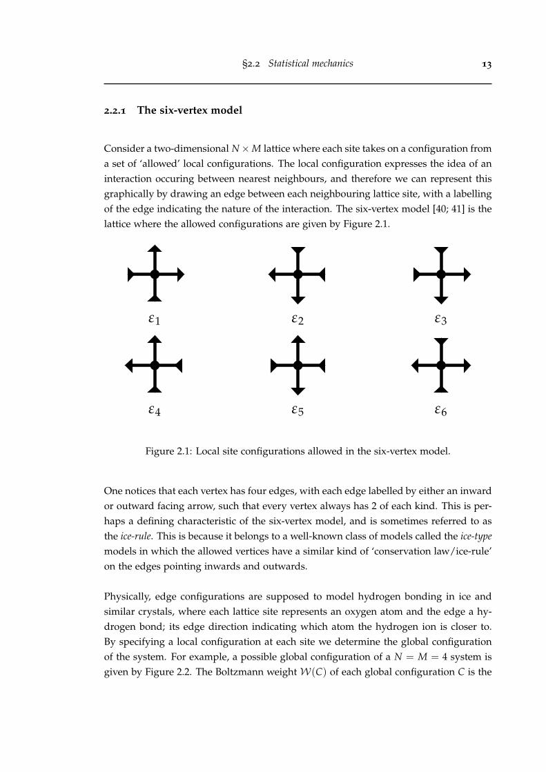
Consider a two-dimensional N×M lattice where each site takes on a configuration froma set of ‘allowed’ local configurations. The local configuration expresses the idea of aninteraction occuring between nearest neighbours, and therefore we can represent thisgraphically by drawing an edge between each neighbouring lattice site, with a labellingof the edge indicating the nature of the interaction. The six-vertex model [40; 41] is thelattice where the allowed configurations are given by Figure 2.1.
ε1 ε2 ε3
ε4 ε5 ε6
Figure 2.1: Local site configurations allowed in the six-vertex model.
One notices that each vertex has four edges, with each edge labelled by either an inwardor outward facing arrow, such that every vertex always has 2 of each kind. This is per-haps a defining characteristic of the six-vertex model, and is sometimes referred to asthe ice-rule. This is because it belongs to a well-known class of models called the ice-typemodels in which the allowed vertices have a similar kind of ‘conservation law/ice-rule’on the edges pointing inwards and outwards.
Physically, edge configurations are supposed to model hydrogen bonding in ice andsimilar crystals, where each lattice site represents an oxygen atom and the edge a hy-drogen bond; its edge direction indicating which atom the hydrogen ion is closer to.By specifying a local configuration at each site we determine the global configurationof the system. For example, a possible global configuration of a N = M = 4 system isgiven by Figure 2.2. The Boltzmann weightW(C) of each global configuration C is the

14 Yang-Baxter Integrability
Figure 2.2: A possible configuration of a 4× 4 six-vertex model with periodic boundaryconditions.
product of the weights appearing locally. In the six-vertex model we assign the energiesε i to vertices as in Figure 2.1, then the local weights are defined by
Wi = exp(− ε i
kT). (2.2.5)
Let us consider Figure 2 as an example. Let us label this configuration as C1. ItsBoltzmann weight can be expressed as
W(C1) =W1W2W23W2
4W55W5
6 . (2.2.6)
As discussed earlier to solve this model we need to be able to sum over the weightsof all possible configurations - the partition function. A popular way to express thiscomplicated summation is with a mathematical object known as the transfer matrix.
2.2.2 The transfer matrix
The problem of computing the partition function can be posed as an eigenvalue prob-lem of a matrix which is often referred to as a transfer matrix. In this section we willshow how the transfer matrix is constructed, techniques used to find its eigenvalues
§2.2 Statistical mechanics 15
Ri′,j′
i,j = i
j
i′
j′
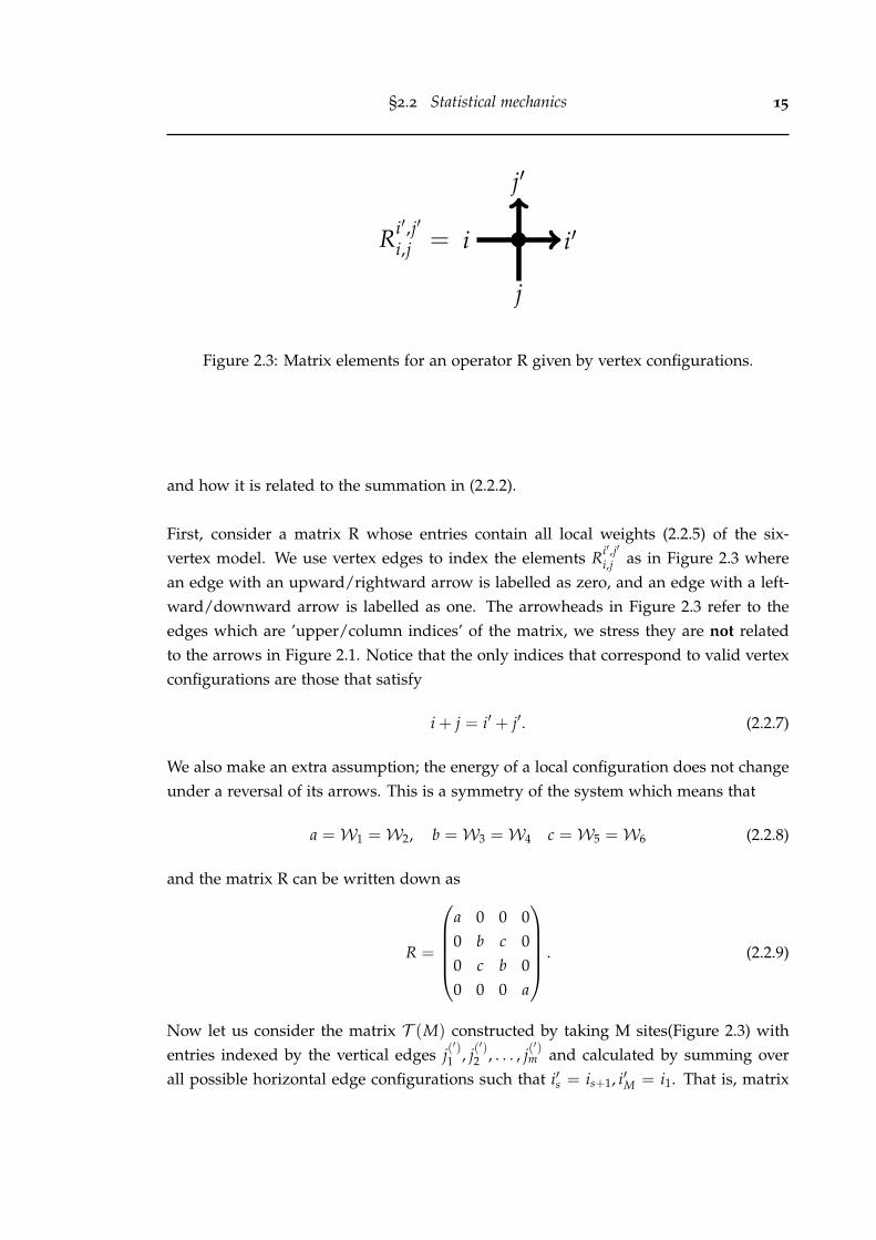
Figure 2.3: Matrix elements for an operator R given by vertex configurations.
and how it is related to the summation in (2.2.2).
First, consider a matrix R whose entries contain all local weights (2.2.5) of the six-vertex model. We use vertex edges to index the elements Ri′,j′
i,j as in Figure 2.3 wherean edge with an upward/rightward arrow is labelled as zero, and an edge with a left-ward/downward arrow is labelled as one. The arrowheads in Figure 2.3 refer to theedges which are ’upper/column indices’ of the matrix, we stress they are not relatedto the arrows in Figure 2.1. Notice that the only indices that correspond to valid vertexconfigurations are those that satisfy
i + j = i′ + j′. (2.2.7)
We also make an extra assumption; the energy of a local configuration does not changeunder a reversal of its arrows. This is a symmetry of the system which means that
a =W1 =W2, b =W3 =W4 c =W5 =W6 (2.2.8)
and the matrix R can be written down as
R =
a 0 0 00 b c 00 c b 00 0 0 a
. (2.2.9)
Now let us consider the matrix T (M) constructed by taking M sites(Figure 2.3) withentries indexed by the vertical edges j(
′)1 , j(
′)2 , . . . , j(
′)m and calculated by summing over
all possible horizontal edge configurations such that i′s = is+1, i′M = i1. That is, matrix

16 Yang-Baxter Integrability
T j′1,...,j′Mj1,...,jM
=
j1
j′1
j2
j′2
jM−1
j′M−1
jM
j′M
Figure 2.4: Graphical notation of the row-to-row transfer matrix T for M sites.
elements have the form
[T (M)]j′1,...,j′Mj1,...,j′M
= ∑i1,...,iM
M
∏s=1
Ri′s,j′sis,js . (2.2.10)
The expression (2.2.10) is somewhat awkward to use in discussions. Quite often wefind it more convenient to use a graphical notation to express complicated objects suchas T which we feel better illustrates its construction from more elementary objects R.We present Figure 2.4 as a graphical representation of (2.2.10). Here external edgesconnected to only one vertex are the matrix indices, and each possible configurationcorresponds to a particular matrix element. Edges that are enclosed by two vertices aresummed over all possible edge states. The loop through all horizontal edges in Figure2.4 means we sum over possible horizontal configurations in determining an elementof the matrix T . Let us note that in imposing periodic boundary conditions, we arediscussing a special case of the six-vertex model on a torus.
The graphical notation we have used in Figure 2.3 and 2.4 is essentially the Penrosegraphical notation used in multilinear algebra. Of course, R and T are multidimensionalarrays and can be thought of as tensor objects with an underlying basis. The order ofa tensor is number of indices needed to specify an element of the array - graphicallythe number of edges passing through the vertex. So R is an order 4 tensor and T isan order 2M tensor. Because the number of lower indices (incoming edges) is equal tothe number of upper indices (outgoing edges), R is a multilinear operator acting on avector space V1 ⊗V2 and likewise for T (but with M factors).
With the machinery we have established so far, it is not hard to see that the partitionfunction Z for the N ×M six vertex model is given by
Z = Trace[T N(M)]. (2.2.11)

§2.3 Yang-Baxter integrability 17
In (2.2.11) we have matrix multiplied N copies of T (M) which sums over all possiblevertical edge configurations except at the lattice boundary. The trace imposes periodicboundary conditions for the boundary edges and sums over all their possible configu-rations. The result is the partition function.
It is well known that the trace of a linear operator is a sum of its eigenvalues. If weknow the eigenvalues of T then we know it for any power of T and therefore we knowZ . Therefore the problem of solving a vertex model is equivalent to diagonalising T -thereby calculating its eigenspectrum.
2.3 Yang-Baxter integrability
There are two main approaches to calculating the spectrum of T ; the Bethe Ansatzand the method of Commuting Transfer matrices. These methods are actually equivalentin a way that was made precise through the Baxter Q-Operators but we will save thatdiscussion for later. Now we will give an overview of the two techniques and introducethe Yang-Baxter equation.
2.3.1 Bethe ansatz
The Bethe ansatz was a method introduced by Hans Bethe [42] to solve the spin-1/2 1DHeisenberg spin by diagonalising its Hamiltonian. Lieb [40] discovered that this tech-nique also works for the six-vertex model, and was able to solve it for a number of cases.
The Bethe ansatz aims to solve the eigenvalue equation
T |X〉 = Λ |X〉 (2.3.1)
directly by assuming the eigenvectors are given by a superposition of plane-waves, thatis
|X〉 = ∑σ
Aσexp(iσk ·X). (2.3.2)
where the sum is over all permutations σ of the components in the wavevector k. Thisspecial form of the eigenvectors is the ’ansatz’ and substituting (2.3.2) into the left-handside of (2.3.1) leads to the right-hand side plus a collection of extra terms. Requiring

18 Yang-Baxter Integrability
that these terms cancel leads to a set of equations for the coefficients Aσ and wavevectorcomponents ks commonly known as the Bethe Ansatz equations.
The ice-rule mentioned in the last section plays an important role in applying (2.3.1)to the six-vertex model. It is easy to see that rule (2.2.7) for each site implies a globalrule
j1 + · · ·+ jM = j′1 + · · ·+ j′M = n (2.3.3)
for the M-site transfer matrix T . Therefore T has a M+1 block-diagonal form and indiagonalising it one can restrict the problem to each block indexed by n =0,. . . ,M. Oncea block n is fixed a state |X〉 is specified by X = (x1, . . . , xn) where xi is the position ofthe ith down configuration in the lattice/one index in T . The sum in (2.3.2) is over then! permutations of k = (k1, . . . , kn).
Peforming the necessary computations one finds that the extra terms in (2.3.1) dis-appear provided that
exp(iMk j) = (−1)n−1n
∏l=1
1− 2∆exp(iMk j) + exp(iM(k j + kl))
1− 2∆exp(iMkl) + exp(iM(k j + kl)), (2.3.4)
∆ := (a2 + b2 − c2)/2ab. (2.3.5)
(2.3.4) are the Bethe ansatz equations for the six-vertex model. They are a set of nequations determining k. Once they are solved, Aσ and Λn in (2.3.1) can be computedby
Aσ = εσ ∏1≤i<j≤n
(1− 2∆exp(iMσi) + exp(iM(σi + σj))
), (2.3.6)
Λn = aMn
∏s=1
L(ks) + bMn
∏s=1
M(ks), (2.3.7)
L(ks) =ab− (c2 − b2)exp(iMks)
a2 − abexp(iMks), (2.3.8)
M(ks) =a2 − c2 − abexp(iMks)
ab− b2exp(iMks). (2.3.9)
Clearly (2.3.4) are transcendental equations and therefore no closed-form solution ex-ists. In fact, these equations remain unsolved for general finite n,M. The only casewhere they have been solved exactly is in the (thermodynamic) limit M→ ∞, and onlyfor the maximum eigenvalue. Perhaps this is fortunate, because for the N ×M lattice

§2.3 Yang-Baxter integrability 19
in the limit M, N → ∞
Z ∼ ΛNMAX, (2.3.10)
so we can say the infinite six-vertex model on a torus can be solved by the Bethe ansatz.At this point we remind the reader of the many-body problem outlined in the last sec-tion. Certainly, the Bethe ansatz equations are in a sense ’equations of motion’ for thesix-vertex model - describing its behaviour on average. It seems counter intuitive thatthe equations for finitely many bodies are harder to solve than for infinitely many in-teracting bodies. Nevertheless, in principle the Bethe ansatz equations admit enoughsolutions k to determine all eigenvalues and eigenvectors of the transfer matrix.
An important point that we want to make is that this method relied on the ice ruleto specify states and the terms in the eigenfunction (2.3.2) by co-ordinates X. For thisreason this technique has come to be known as the coordinate Bethe ansatz. However,it is not immediately clear how one could apply this technique if such a conservationrule does not exist. This is a problem encountered in solving the eight-vertex model.Regardless, the eight-vertex model was solved by Baxter [43] using what has come tobe known as the commuting transfer matrix method.
2.3.2 Commuting transfer matrices
These two methods on the surface seem quite different but they actually imply oneanother. That is, the Bethe ansatz equations imply that transfer matrices with differentBoltzmann weights commute. Conversely, the premise of commuting transfer matricesimplies the Bethe ansatz equations. This fact allows a more algebraic formulation of thecoordinate bethe ansatz approach outlined in the last section. The Yang-Baxter equationarises as a sufficiency condition for the commutativity of transfer matrices and thereforethe existence of the Bethe ansatz equations.
The crucial observation to make is that the Boltzmann weights a,b,c of equation (2.2.8)only enter the Bethe ansatz equations (2.3.4) through ∆ (2.3.5) and therefore this isthe only variable the eigenvectors depend on. That means that if we choose differentweights a′, b′, c′ with the same ∆ then the transfer matrix has the same set of eigenvec-tors. At this point it is appropriate to introduce a parametrisation of the weights. Let

20 Yang-Baxter Integrability
us define
a = ρq(1− λ2), b = ρ(q2 − λ2), c = ρ(q2 − 1)λ, (2.3.11)
∆ =q + q−1
2(2.3.12)
so that a,b,c are entire functions of q, λ. For fixed q, the Boltzmann weights a(λ), b(λ),c(λ) lie on a curve parametrised by λ. For every point we can associate a transfermatrix T (λ). Every transfer matrix lying on this curve will have the same eigenvectorsbecause ∆ depends only on q. Therefore they are simultaneously diagonalisable andhence commute.
[T (λ), T (µ)] = 0 ∀λ, µ ∈ C. (2.3.13)
Now supposing that (2.3.13) holds it is possible to recover the Bethe ansatz equations.The approach is to construct operators Q(λ) that satisfy
T (λ)Q(λ) =[λq−1
]MQ(qλ) + [λ]MQ(q−1λ), (2.3.14)
[T (λ),Q(µ)] = [Q(λ),Q(µ)] = 0. (2.3.15)
(2.3.14) is known as the Baxter TQ-relation. The commutativity (2.3.15) of these opera-tors with the transfer matrix means that they same have the eigenvectors and so can wediagonalize them simultaneously. Define diagonal matrices Td(λ) and Qd(λ) by
T (λ) =M−1Td(λ)M, Q(λ) =M−1Qd(λ)M (2.3.16)
then the TQ-relation becomes 2M equations of the form
Λ(λ) =
[λq−1]MA(qλ) + [λ]MA(q−1λ)
A(λ) (2.3.17)
for each entry on the main diagonal Td(λ)Qd(λ) and eigenvaluesΛ(λ),A(λ) respec-tively. Λ(λ) is an entire function in λ by (2.3.16) since M does not depend on λ andT (λ) is entire. Therefore the right-hand side of (2.3.17) is entire. This means that givenzeroes λj of A(λ) the numerator must also vanish, therefore
[λj]M[
λjq−1]M = −
A(qλj)
A(q−1λj)(2.3.18)

§2.3 Yang-Baxter integrability 21
S(λ, µ)i′,j′′,k′
i,j,k =
j
j′′
k k′
i i′
Figure 2.5: Matrix [S(λ, µ)]
which are equivalent to the Bethe ansatz equations (2.3.4). To make the connection weidentify
exp(ik j) =
[λj][
λjq−1] , A(λ) =
n
∏l=1
[λλ−1
l
](2.3.19)
and so the solutions k j of (2.3.4) correspond to solutions λj of (2.3.18).
Of course the argument rests upon the assumption that transfer matrices commutefor all values of the spectral parameter - it may not be true. But even if it is true it is notclear from the arguments how one could construct Q(λ) if the Bethe-ansatz equationswere not already known. The problem of constructing Q-operators has been consid-ered in many texts, beginning with Baxter in [43] for eight-vertex model, known asthe propagation through the vertex method. Another method due to Bazhanov-Lukyanov-Zamalodchikov is given in [44; 45] and yet another method by Chicherin-Derkachov-Karakhanyan in [46; 27; 47].
On the problem of commuting transfer matrices, we may ask, what is a sufficient con-dition for (2.3.13) to hold? Consider a matrix S(λ, µ) with elements defined by
[S(λ, µ)]i′,j′′,k′
i,j,k := ∑j′
R(λ)i′,j′
i,j R(µ)k′,j′′
k,j′ (2.3.20)
and represented graphically in Figure 2.5. We can write T (µ)T (λ) and T (λ)T (µ) interms of S . It is obvious that
[T (λ)T (µ)]j′′1 ,...,j′′M
j1,...,jM= Trace
M
∏k=1
[S(λ, µ)]j′′kjk
(2.3.21)
22 Yang-Baxter Integrability
j
j′′
k
k′′
i
i′′
=R R
R(λ)
R(µ)
R(µ)
R(λ)
j
j′′
k
k′′i
i′′
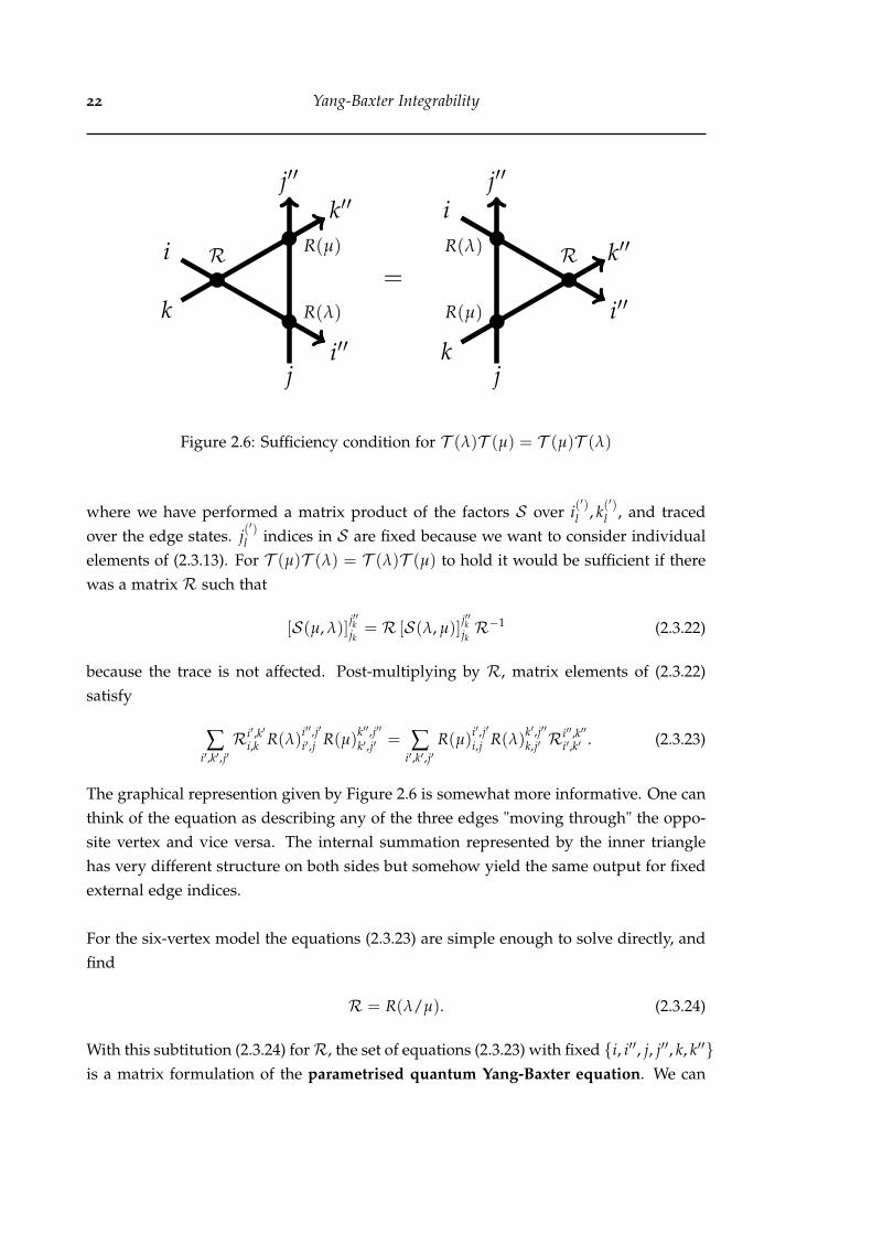
Figure 2.6: Sufficiency condition for T (λ)T (µ) = T (µ)T (λ)
where we have performed a matrix product of the factors S over i(′)
l , k(′)
l , and tracedover the edge states. j(
′)l indices in S are fixed because we want to consider individual
elements of (2.3.13). For T (µ)T (λ) = T (λ)T (µ) to hold it would be sufficient if therewas a matrix R such that
[S(µ, λ)]j′′kjk= R [S(λ, µ)]
j′′kjkR−1 (2.3.22)
because the trace is not affected. Post-multiplying by R, matrix elements of (2.3.22)satisfy
∑i′,k′,j′Ri′,k′
i,k R(λ)i′′,j′
i′,j R(µ)k′′,j′′
k′,j′ = ∑i′,k′,j′
R(µ)i′,j′
i,j R(λ)k′,j′′
k,j′ Ri′′,k′′i′,k′ . (2.3.23)
The graphical represention given by Figure 2.6 is somewhat more informative. One canthink of the equation as describing any of the three edges "moving through" the oppo-site vertex and vice versa. The internal summation represented by the inner trianglehas very different structure on both sides but somehow yield the same output for fixedexternal edge indices.
For the six-vertex model the equations (2.3.23) are simple enough to solve directly, andfind
R = R(λ/µ). (2.3.24)
With this subtitution (2.3.24) forR, the set of equations (2.3.23) with fixed i, i′′, j, j′′, k, k′′is a matrix formulation of the parametrised quantum Yang-Baxter equation. We can

§2.3 Yang-Baxter integrability 23
now introduce it formally.
Definition 2.3.0.1 (Quantum Yang-Baxter equation). The linear operator equality
R12(λ)R13(λµ)R23(µ) = R23(µ)R13(λµ)R12(λ), (2.3.25)
acting on the vector space V1⊗V2⊗V3 is the quantum Yang-Baxter equation. A solutionR(λ) is a linear ’R-operator’ acting on W ⊗U such that Rij(λ) acts as W = Vi, U = Vj
and trivially in the third space.
The relation (2.3.25) is probably the most common presentation of the Yang-Baxterequation found in the literature. We refer to solutions R(λ) as R-operators when dis-cussing them independent of a basis. Of course, if we choose an orthonormal basis|i, j〉 := |i〉 ⊗ |j〉 ∈ W ⊗U then the operator can be realised as a R-matrix R(λ) withelements
R(λ)i′,j′
i,j = 〈i, j| R(λ) |i′, j′〉 (2.3.26)
and (2.3.25) can be written as (2.3.23) with (2.3.24) and re-scaling λ := λµ.
Figure 2.6 illustrates clearly how R in (2.3.25) are composed with each other. Thethree edges spanned by i, i′′, j, j′′, k, k′′ represent the action in each factor ofV1 ⊗ V2 ⊗ V3. With a basis (2.3.26) the Yang-Baxter equation expresses an equality oftwo 6-order tensors.
Using operator language, we can reformulate the transfer matrix (2.2.10)/Figure 2.4as a ‘global’ operator
T (λ) := TraceV0 [M0(λ)] , (2.3.27)
M0(λ) := R01(λ)⊗R02(λ)⊗ · · · ⊗R0M(λ) (2.3.28)
acting in the space V1 ⊗ · · · ⊗ VM. This is sometimes referred to as the quantum space.The operatorM0(λ) is called the Monodromy operator and the transfer matrix is formedby taking the trace over V0 also known as the auxiliary space. Graphically, it is fairly easyto see that
R12(λ/µ)M1(λ)M2(µ) =M2(µ)M1(λ)R12(λ/µ) (2.3.29)
by starting with the left hand side and moving R ’through’ each lattice site swappingλ and µ as in Figure 2.6. If R is non-singular (2.3.29) implies (2.3.13) so this relation is

24 Yang-Baxter Integrability
somehow a more general statement. R can be thought of as ’intertwining’ representa-tions of M, in the sense of a module homomorphism preserving the action of M onsome representation space. We will elaborate on this later.
Some parallels appear to emerge between integrability in the Liouville sense and inthe Yang-Baxter sense. Just as a Liouville integrable system in classical mechanics ad-mit sufficiently many commuting conserved quantities, a Yang-Baxter integrable sys-tem in statistical mechanics admits infinitely many commuting transfer matrices. TheYang-Baxter equation is a sufficiency condition for commutativity and therefore eachR-matrix solution encodes a model in statistical mechanics that is exactly solvable bythe Bethe ansatz/Q-operators. A straightforward decoding of the R-matrix is to inter-pet its elements as Boltzmann weights of a vertex model just like (2.2.9) and Figure2.1. Obviously not all solvable models are posed as vertex models and the process ofrelating such to an R-matrix can be highly non-trivial. The details are not important inour work, we only remark that Yang-Baxter integrability is not always obvious and canbe hidden.
The question we want to answer is; How to solve the Yang-Baxter equation? Howto construct R-matrices?. In this thesis we have constructed R-matrix solutions to theYang-Baxter equation using a variety of methods. It is an interesting walkthrough ofdifferent approaches to constructing matrix elements, which all produce the same re-sults. We are also interested in the structure of the solutions, and we find that thesolutions have an interesting form in terms of hypergeometric series, relating them tocertain special classes of orthogonal polynomials. We also find some more elementaryobjects related to the R-matrix. All R-matrices in this thesis are related to a special classof algebras known as ’quantum groups’, which we will introduce now.
2.4 Quantum groups
Quantum groups were first found by the Leningrad school under Ludwig Fadeev as aconsequence of their approach known as the quantum inverse scattering method [48; 5; 49]to constructing and solving integrable systems. They were introduced formally byDrinfel’d [50; 51] and Jimbo [16] as Hopf algebras with extra structure that makes themquasitriangular. Roughly speaking, each algebra contains the symmetries of an entireclass of R-matrices [52; 53]. Given such an algebra, it is usually possible to constructan element of the algebra that represents this class - the so-called universal R-matrix

§2.4 Quantum groups 25
[50; 54; 55; 56; 3; 57]. Applying a representation of the algebra to the universal R-matrixallows one to realise it as an actual matrix.
Many of these algebras are deformations of Universal enveloping algebras U(g) of a Liealgebra g. This unexpected link between statistical mechanics and Lie algebras was per-haps the reason for so much research interest over the past few decades. To show howquantum groups arise in studying R-matrices we will give an overview of some of thesteps involved in the quantum inverse scattering method where they were originallydiscovered.
2.4.1 Quantum inverse scattering method
In the last section we constructed a collection of transfer matrices from the six-vertexmodel and found that they commute. In general, the existence of an invertible matrixR which satisfies the Yang-Baxter equation (2.3.25) was seen to be a sufficient conditionfor commutativity. Now we ask the converse question: given an R-matrix, what kindof commuting transfer matrices can be constructed? That is, we want to solve equation(2.3.22) for fixed R and variable S .
This equation is just a local form of (2.3.29) (or M = 1) for M0 (2.3.28), but this istoo specific because it is built out of factors R. We use a more general form
ML0 (λ) := L01(λ)⊗L02(λ)⊗ · · · ⊗ L0M(λ), (2.4.1)
where the L(λ) are known as Local operators or L-operators. They act in the auxiliaryspace V0 as a n × n matrix with each entry an operator acting in the quantum spaceV1 ⊗ · · · ⊗VM. We also make the assumption that its dependence on λ only enters as
L(λ) = λL+(λ) + λ−1L−(λ) (2.4.2)
where L+(λ) is an upper triangular matrix and λ−1L−(λ) is a lower triangular matrix.For example, when n = 2 it can be written as
L(λ) =(
L−11λ−1 + L+11λ λL12
λ−1L21 L−22λ−1 + L+22λ
), (2.4.3)
a 2× 2 matrix with operator entries Lij. The idea is that a representation of these op-erators will give commuting transfer matrices by construction and hence an integrable

26 Yang-Baxter Integrability
k
k′′
i
i′′
=R12 R12
L13(λ)
L23(µ)
L23(µ)
L13(λ)
k
k′′i
i′′
Figure 2.7: Yang-Baxter RLL-relation
model. Since R satisfies (2.3.22), the equation (2.3.25) can be written as
R12(λ/µ)L13(λ)L23(µ) = L23(µ)L13(λ)R12(λ/µ), (2.4.4)
which is sometimes referred to as the RLL-relation or a weaker RLL-form Yang-Baxterequation. A graphical representation of this equation is given in Figure 2.7
We will also work with an n × n × n × n, n ≥ 2 R-matrix whose elements are givenby the function
[R(λ)]i′,j′
i,j = δi,i′δj,j′δi,j(q− 1)(λ + λ−1q−1) + δi,i′δj,j′(λ− λ−1) + δi,j′δj,i′σi,i′ (2.4.5)
for 1 ≤ i, j, i′, j′ ≤ n and
σi,j =
0 if i = j,
(q− q−1)λ if i < j,
(q− q−1)λ−1 if i > j.
(2.4.6)
For n = 2 this is equivalent to the six-vertex model R-matrix (2.3.24) and (2.2.8) but witha change of variables. Substituting this R-matrix and (2.4.3) in the RLL relation (2.4.4)defines relations for the operators L±αβ. In particular,
[L±αα, L±ββ] = [L+αα, L−ββ] = 0, (2.4.7a)
L±ααLβγ = q∓δαβ±δαγ LβγL±αα, (2.4.7b)
LαβLβα − LβαLαβ = (q− q−1)(L+ααL−ββ − L+
ββL−αα), (2.4.7c)
LαβLαγ = q−εαβγ LαγLαβ n > 2, (2.4.7d)
LαγLβγ = q−εαβγ LβγLαγ n > 2, (2.4.7e)

§2.4 Quantum groups 27
LαβLβγ − LβγLαβ = −εαβγ(q− q−1)Lεαβγ
ββ Lαγ n > 2, (2.4.7f)
LαβLγδ − LγδLαβ = (qεαβγ − qεαβδ)LγβLαδ n > 3 (2.4.7g)
where α, β, γ, δ ∈ 1, . . . , n do not coincide for relations (2.4.7d)− (2.4.7g) and εαβγ isan antisymmetric function such that
εαβγ = 1, if α < β < γ. (2.4.8)
The relations (2.4.7)-(2.4.7g) define the L-operator algebra RL for the R-matrix (2.4.5). RL
also admits the comultiplication ∆ : RL → RL ⊗RL given by
∆(Lαβ) = ∑γ
Lαγ ⊗ Lγβ (2.4.9)
which makes it a Hopf algebra. RL is one presentation of the quantum group com-monly known as Uq(sln) in the literature. If we make the identification
L±ii = q±∑n−1s=1
(n−s)Hsn ∓∑i−1
s=1 Hs , (2.4.10)
Li,i+1 = (q− q−1)q∑n−1s=1
(n−s)Hsn −∑i
s=1 Hs Fi, (2.4.11)
Li+1,i = (q−1 − q)q−∑n−1s=1
(n−s)Hsn +∑i
s=1 Hs Ei (2.4.12)
the defining relations (2.4.7)-(2.4.7g) of the L-operator algebra RL are equivalent to thestandard definition of Uq(sln) introduced independently by Drinfeld and Jimbo. Wewill now formally introduce this quantum group [50; 51; 16] starting with the moregeneral algebra Uq(sln), and explain its reductions.
2.4.2 The quantum group Uq(sln)
Uq(sln) is the algebra generated by elements q±Hi , Ei, Fii=0,...,n−1 over the field of ra-tional functions C(q) subject to the relations
qHi qHj = qHj qHi , qHi q−Hi = q−Hi qHi = 1, (2.4.13a)
qHi Ej = qaij EjqHi , qHi Fj = q−aij FjqHi , (2.4.13b)
[Ei, Fj] = δi,jqHi − q−Hi
q− q−1 , (2.4.13c)
E2i Ej − (q + q−1)EiEjEi + EjE2
i = 0 |i− j| = 1 mod n, (2.4.13d)
F2i Fj − (q + q−1)FiFjFi + FjF2
i = 0 |i− j| = 1 mod n (2.4.13e)
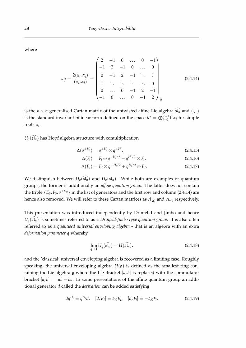
28 Yang-Baxter Integrability
where
aij =2(αi, αj)
(αi, αi)=
2 −1 0 . . . 0 −1−1 2 −1 0 . . . 0
0 −1 2 −1. . .
......
. . . . . . . . . . . . 00 . . . 0 −1 2 −1−1 0 . . . 0 −1 2
ij
(2.4.14)
is the n× n generalised Cartan matrix of the untwisted affine Lie algebra sln and (., .)is the standard invariant bilinear form defined on the space h∗ =
⊕n−1i=0 Cαi for simple
roots αi.
Uq(sln) has Hopf algebra structure with comultiplication
∆(q±Hi) = q±Hi ⊗ q±Hi , (2.4.15)
∆(Fi) = Fi ⊗ q−Hi/2 + qHi/2 ⊗ Fi, (2.4.16)
∆(Ei) = Ei ⊗ q−Hi/2 + qHi/2 ⊗ Ei. (2.4.17)
We distinguish between Uq(sln) and Uq(sln). While both are examples of quantumgroups, the former is additionally an affine quantum group. The latter does not containthe triple E0, F0, q±H0 in the list of generators and the first row and column (2.4.14) arehence also removed. We will refer to these Cartan matrices as A
slnand Asln respectively.
This presentation was introduced independently by Drinfel’d and Jimbo and henceUq(sln) is sometimes referred to as a Drinfeld-Jimbo type quantum group. It is also oftenreferred to as a quantised universal enveloping algebra - that is an algebra with an extradeformation parameter q whereby
limq→1
Uq(sln) = U(sln), (2.4.18)
and the ’classical’ universal enveloping algebra is recovered as a limiting case. Roughlyspeaking, the universal enveloping algebra U(g) is defined as the smallest ring con-taining the Lie algebra g where the Lie Bracket [a, b] is replaced with the commutatorbracket [a, b] := ab− ba. In some presentations of the affine quantum group an addi-tional generator d called the derivation can be added satisfying
dqHi = qHi d, [d, Ei] = δi0Ei, [d, Fi] = −δi0Fi, (2.4.19)

§2.4 Quantum groups 29
∆(d) = d⊗ 1 + 1⊗ d. (2.4.20)
This is because the Cartan matrix has corank 1 and it can be shown that the Cartansubalgebra of the underlying Lie algebra must have dimension n + 1. A further elementc called the central charge is also present, but for our purposes we have set c = 0.
For the sake of completeness, we will give the definition of sln. It is the vector spaceover C generated by Ei, Fi, Hin−1
i=0 with Lie Bracket [·, ·] such that
[Hi, Hj] = 0, [Ei, Fj] = δi,jHi, (2.4.21a)
[Hi, Ej] = aijEj, [Hi, Fj] = −aijFj, (2.4.21b)
ad1−aijEi
(Ej) = 0, ad1−aijFi
(Fj) = 0 (2.4.21c)
where aij is given in (2.4.14). sln is an infinite dimensional affine lie algebra. It canbe identified as sln ∼= sln ⊗ C[t, t−1]⊕ Cc ⊕ Cd for finite dimensional sln and Laurentpolynomials C[t, t−1]. Just like the quantum case, we can have extra elements c and dwith relations analogous to (2.4.19). They generalise the Lie algebra to what is knownas an affine Kac-Moody algebra. Our presentation corresponds to the case c = 0.
It is well known that finite semisimple Lie algebras g admit the vector space decom-position
g = g∆− ⊕ h⊕ g∆+ , (2.4.22)
g∆± =⊕
λ∈∆±
gλ, (2.4.23)
gλ = X ∈ g | [H, X] = λ(H)X ∀H ∈ h (2.4.24)
where h is called the Cartan subalgebra and is the maximal commutative subalgebra ofg. g∆± are the positive and negative root spaces corresponding to roots λ ∈ h∗. Roots arecharacterised in terms of simple roots αin
i=1 where n is the rank of the algebra. Eachroot is an integral sum of simple roots λ = ∑i Ciαi, Ci ∈ Z and form the root system
∆ = ∆+ ∪ ∆−, (2.4.25)
which splits into ‘positive’ roots ∆+ or ‘negative’ roots ∆− depending on the sign Ci
which are either all positive or all negative. The entire root system can be constructedfrom the simple roots through the Weyl group although the details are not important tous here. The root vector Eλ corresponding to the root λ can be constructed from the

30 Yang-Baxter Integrability
generators in (2.4.21) by
Eαi = Ei, E−αi = Fi, Hαi = Hi, i ≥ 1
[Eαi , E−αi ] = Hαi [Eα, Eβ] = µαβEα+β for α + β 6= 0, µαβ ∈ Q. (2.4.26)
The root vectors form a basis of the Lie algebra, sometimes called the Cartan-Weyl basisof the Lie algebra. With normalisation µαβ ∈ Z it also sometimes called a Chevalleybasis. For sln the dimension of the Lie algebra is n2 − 1.
The infinite dimensional affine Lie algebra g case has a similar root space decompo-sition as (2.4.22) except the root system (2.4.25) is infinite because of the addition of anextra simple root α0. The write the system down, we first locate the unique maximalroot θ ∈ ∆g
+ of the finite algebra g and note that it satisfies
a0i = −2(θ, αi)
(θ, θ), ai0 = −2
(αi, θ)
(αi, αi)(2.4.27)
where maximal is defined as being the root whereby θ − γ /∈ ∆g− ∀γ ∈ ∆g
+. For sln it isnot too hard to see that θ = ∑n−1
i=1 αi.
Next we define δ := α0 + θ which is also the null root of the affine Lie algebra andsatisfies
(δ, δ) = 0, (δ, θ) = (θ, δ) = 0 (2.4.28)
then the root system ∆g+ of the affine Lie algebra g can be written down as
∆g+ = γ + mδ | γ ∈ ∆g
+, m ∈ Z+ ∪ mδ | m ∈ Z+
∪ (δ− γ) + mδ | γ ∈ ∆g+, m ∈ Z+ (2.4.29)
and similarly for the negative root system ∆g+.
The corresponding root vectors can be constructed similar to (2.4.26) for the Lie al-gebra but we are interested in analogous elements of the quantum group which reduceto the Lie algebra root vectors in the limit q → 1. Therefore we will only give theconstruction in the quantum case. To do this, we must first choose an ordering of thepositive roots in (2.4.29). We choose the normal ordering
α ≺ α + β ≺ β, ∀α, β ∈ ∆g+, (2.4.30)
§2.4 Quantum groups 31
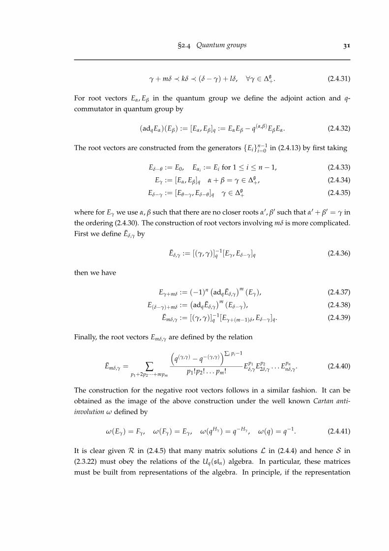
γ + mδ ≺ kδ ≺ (δ− γ) + lδ, ∀γ ∈ ∆g+. (2.4.31)
For root vectors Eα, Eβ in the quantum group we define the adjoint action and q-commutator in quantum group by
(adqEα)(Eβ) := [Eα, Eβ]q := EαEβ − q(α,β)EβEα. (2.4.32)
The root vectors are constructed from the generators Ein−1i=0 in (2.4.13) by first taking
Eδ−θ := E0, Eαi := Ei for 1 ≤ i ≤ n− 1, (2.4.33)
Eγ := [Eα, Eβ]q α + β = γ ∈ ∆g+, (2.4.34)
Eδ−γ := [Eθ−γ, Eδ−θ ]q γ ∈ ∆g+ (2.4.35)
where for Eγ we use α, β such that there are no closer roots α′, β′ such that α′+ β′ = γ inthe ordering (2.4.30). The construction of root vectors involving mδ is more complicated.First we define Eδ,γ by
Eδ,γ := [(γ, γ)]−1q [Eγ, Eδ−γ]q (2.4.36)
then we have
Eγ+mδ := (−1)n (adqEδ,γ)m
(Eγ), (2.4.37)
E(δ−γ)+mδ :=(adqEδ,γ
)m(Eδ−γ), (2.4.38)
Emδ,γ := [(γ, γ)]−1q [Eγ+(m−1)δ, Eδ−γ]q. (2.4.39)
Finally, the root vectors Emδ,γ are defined by the relation
Emδ,γ = ∑p1+2p2···+mpm
(q(γ,γ) − q−(γ,γ)
)∑i pi−1
p1!p2! . . . pm!Ep1
δ,γEp22δ,γ . . . Epn
nδ,γ. (2.4.40)
The construction for the negative root vectors follows in a similar fashion. It can beobtained as the image of the above construction under the well known Cartan anti-involution ω defined by
ω(Eγ) = Fγ, ω(Fγ) = Eγ, ω(qHγ) = q−Hγ , ω(q) = q−1. (2.4.41)
It is clear given R in (2.4.5) that many matrix solutions L in (2.4.4) and hence S in(2.3.22) must obey the relations of the Uq(sln) algebra. In particular, these matricesmust be built from representations of the algebra. In principle, if the representation

32 Yang-Baxter Integrability
theory of the underlying algebra is understood then matrix solutions to (2.4.4) can beconstructed.
Of course, the RLL-relation (2.4.4) is a weaker form of the Yang-Baxter equation (2.3.25)which is what we are interested in solving. Therefore solutions L must also describethe R-Operator solutions R and therefore we expect the quantum group Uq(sln) alsodescribes the structure of the R-matrix. In deriving the L-operator algebra RL (2.4.7)-(2.4.7g) each side of (2.4.4) acting in the third space V3 of V1 ⊗ V2 ⊗ V3 was left asan abstract operator. In trying to solve (2.3.25) we could do the same thing insteadwith spaces V1 or V2 and derive the same algebra relations due to the symmetry ofthe equation. Therefore an operator R ∈ End(V ⊗U) solving (2.3.25) acts with samequantum group structure in both spaces, and is some representation of an elementR ∈ Uq(sln)⊗Uq(sln) which often referred to as the universal R-matrix. That is,
R = (πV ⊗ πW)(R) (2.4.42)
where πV : Uq(sln) → End(V) is a representation associates each element of the quan-tum group with a linear transformation on a representation space V. The Cartan-Weylbasis construction is useful because it turns out they ‘building blocks’ of the universalR-matrix - it can be written down explicitly in terms of the root vectors, which we willdo in the next section.
In this section we started with an R-matrix (2.4.5) and showed that it has underly-ing Uq(sln) structure. It turns out that this matrix is only one instance of a large familyof matrices encapsulated by the Uq(sln) universal R-matrix R. It corresponds to thefundamental symmetric tensor representation of R which we will elaborate upon furtherwhen we discuss the representation theory of Uq(sln).
It seems that we can construct many new matrix solutions to the Yang-Baxter equationby starting with a universal R-matrix and ’simply’ evaluating it for different represen-tations as in (2.4.42). In principle this is doable for Uq(sln) as the universal R-matrixis known and the representation theory is well understood. Unfortunately the expres-sion for the universal R-matrix is quite complicated and direct evaluation has so faronly been successful for small n in low dimensional representations [1; 2]. A majorresult of this thesis is the construction of matrix solutions for all n and for higher finitedimensional and infinite dimensional representations. We do this by exploring somedifferent methods of constructing R-matrices and show they are more efficient than di-rect evaluation of the universal R-matrix. Regardless, we find it appropriate to give the
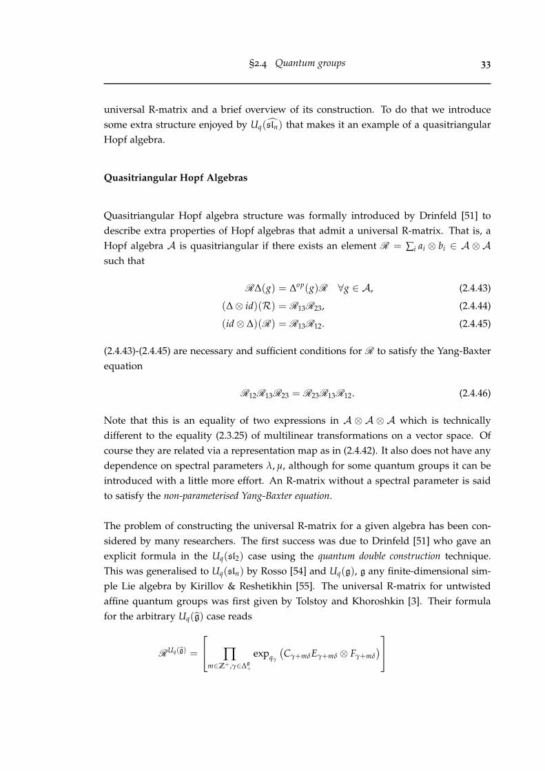
§2.4 Quantum groups 33
universal R-matrix and a brief overview of its construction. To do that we introducesome extra structure enjoyed by Uq(sln) that makes it an example of a quasitriangularHopf algebra.
Quasitriangular Hopf Algebras
Quasitriangular Hopf algebra structure was formally introduced by Drinfeld [51] todescribe extra properties of Hopf algebras that admit a universal R-matrix. That is, aHopf algebra A is quasitriangular if there exists an element R = ∑i ai ⊗ bi ∈ A ⊗ Asuch that
R∆(g) = ∆op(g)R ∀g ∈ A, (2.4.43)
(∆⊗ id)(R) = R13R23, (2.4.44)
(id⊗ ∆)(R) = R13R12. (2.4.45)
(2.4.43)-(2.4.45) are necessary and sufficient conditions for R to satisfy the Yang-Baxterequation
R12R13R23 = R23R13R12. (2.4.46)
Note that this is an equality of two expressions in A ⊗ A ⊗ A which is technicallydifferent to the equality (2.3.25) of multilinear transformations on a vector space. Ofcourse they are related via a representation map as in (2.4.42). It also does not have anydependence on spectral parameters λ, µ, although for some quantum groups it can beintroduced with a little more effort. An R-matrix without a spectral parameter is saidto satisfy the non-parameterised Yang-Baxter equation.
The problem of constructing the universal R-matrix for a given algebra has been con-sidered by many researchers. The first success was due to Drinfeld [51] who gave anexplicit formula in the Uq(sl2) case using the quantum double construction technique.This was generalised to Uq(sln) by Rosso [54] and Uq(g), g any finite-dimensional sim-ple Lie algebra by Kirillov & Reshetikhin [55]. The universal R-matrix for untwistedaffine quantum groups was first given by Tolstoy and Khoroshkin [3]. Their formulafor the arbitrary Uq(g) case reads
RUq(g) =
∏m∈Z+,γ∈∆g
+
expqγ
(Cγ+mδEγ+mδ ⊗ Fγ+mδ
)

34 Yang-Baxter Integrability
× exp
(∑
m∈Z+
r
∑i,j=1
Sm,ijEmδ,αi ⊗ Fmδ,αj
)
×
∏m∈Z+,γ∈∆g
+
expqγ
(C(δ−γ)+mδE(δ−γ)+mδ ⊗ F(δ−γ)+mδ
)× exp
(h
r
∑i,j=1
bijhαi ⊗ hαj
)(2.4.47)
where r is the rank of the Cartan matrix Ag and the factors Cγ, Sm,ij, bij are determinedby the relations
[Eγ, Fγ] =qHγ − q−Hγ
Cγ, bij =
(A−1
g
)ij
, q = exp(h), (2.4.48)
Sm,ij =(
T−1m
)ij
, Tm,ij = (−1)mδij m−1 qm(αi ,αj) − q−m(αi ,αj)
(qαi − q−1αi )(qαj − q−1
αj ). (2.4.49)
The ordering of the products follows the normal ordering of the roots given in (2.4.31).For example, in the case of Uq(sl2) the Khoroshkin-Tolstoy formula for the universalR-matrix reads
RUq(sl2) =
(∏n≥0
expqα((q− q−1)(Eα+nδ ⊗ Fα+nδ))
)
× exp
(∑n≥0
n[n]−1qα(qα − q−1
α )(Enδ ⊗ Fnδ)
)
×(
∏n≥0
expqα((q− q−1)(E(δ−α)+nδ ⊗ F(δ−α)+nδ))
)q
12 Hα⊗Hα . (2.4.50)
As mentioned earlier, the universal R-matrix does not typically have a spectral param-eter. For Uq(sln) a spectral parameter can be introduced by the well known evaluationhomomorphism map [58] evalx : Uq(sln)→ Uq(sln)⊗C[x, x−1] by
R(x, y) = (evalx ⊗ evaly)(R), (2.4.51)
evalx(E0) = xGFθ , evalx(F0) = x−1G−1Eθ , evalx(qH0) = q−Hθ ,
evalx(Ei) = Ei, evalx(Fi) = Fi, evalx(qHi) = qHi , 1 ≤ i ≤ n− 1 (2.4.52)
where G := q1n ∑n−1
i=1 (n−2i)Hi . Applying (2.4.51) to (2.4.47) one can check that the universalR-matrix with spectral parameter depends only on the difference of the parameterssuch that R(x, y) = R(x/y). Such an element, by construction, is a solution to the

§2.4 Quantum groups 35
parameterised Yang-Baxter equation
R12(λ)R13(λµ)R23(µ) = R23(µ)R13(λµ)R12(λ). (2.4.53)
Now that we have a formula (2.4.47), (2.4.51) for a universal R-matrix with spectralparameter we could evaluate it directly for a given representation as in (2.4.42). Asmentioned earlier this is a problem that has not been solved in general. In this thesiswe will show that there are many other ways to evaluate this quantum group formulathat are not only more efficient but reveal interesting structure of the R-matrix that isnot obvious by focusing solely on the Khoroskin-Tolstoy construction.
In the next section we will discuss the representation theory of Uq(sln) in the genericq case which is well understood. The classification of all representations of the alge-bra gives a classification of all matrix realisations of R(λ) and hence solutions to theYang-Baxter equation with sln structure.
Representation Theory
Given the isomorphism g ∼= g⊗ C[x, x−1]⊕ Cc⊕ Cd well known in the study of non-twisted affine Kac-Moody Lie algebras, one asks if a similar isomorphism exists forquantum groups Uq(g). Unfortunately it does not, except only for sln where the evalu-ation homomorphism map (2.4.52) shows that
Uq(sln) ∼= Uq(sln)⊗C[x, x−1] (2.4.54)
where the left-hand side is as we have presented it in (2.4.13) ignoring the elementsc and d. This means that the extra generators E0, F0, H0 of Uq(sln) exist insideUq(sln)⊗C[x, x−1] and that representations πV : Uq(sln)→ End(V) can be constructedby considering representations πV : Uq(sln) → End(V) of the non-affine algebra andpulling back by evalx. That is,
πV = πV evalx, (2.4.55)
and so in discussing the Uq(sln) R-matrix with spectral parameter one is really takingabout the Uq(sln) R-matrix. The only other parameters needed to specify an R-matrixare the parameters fixing the underlying quantum group representation, and in thiscase the non-affine quantum group. We will not say anything about the representationtheory of Uq(g) in general other than that irreducible representations can be constructed

36 Yang-Baxter Integrability
by "combining" irreducible representations of the non-affine quantum group in a man-ner that is highly technical and non-trivial.
We will assume that q is not a root of unity. In this case the irreducible representa-tions of Uq(sln) are classified by highest weight representations. These are determined bythe linear functional
I =n−1
∑s=1
Isωs, Is ∈ C (2.4.56)
on the Cartan subalgebra h where ωs have the the action
ωi(Hj) = δi,j. (2.4.57)
For now we choose to only focus on the theory for the case I = Iω1 for I ∈ Z+ alsoknown as symmetric tensor representations and from now on we will refer to a specificrepresentation by its single parameter ‘I’ or map π I , and its underlying representationspace VI . This is because much of the thesis is dedicated to R-matrices in these repre-sentations. The theory in this case is treated explicitly in Chapter 5 of [59] where theunderlying space is characterised as the subspace of homogenous polynomials in thering C[X1, X2, . . . , Xn] with basis
|m1, m2, . . . , mn〉 =Xm1
1[m1]q!
Xm22
[m2]q!. . .
Xmnn
[mn]q!, (2.4.58)
such that I ≥ m1, m2, . . . , mn ≥ 0 and ∑s ms = I. This basis generates a space ofdimension (I+n−1
n−1 ) which we denote by VI . Quantum group generators K±i , Ei, Fi, i =
1, 2, . . . n presented in [59] act on this basis by
Ki |m1, m2, . . . , mn〉 = qmi−mi+1 |m1, m2, . . . , mn〉 , (2.4.59a)
Ei |m1, m2, . . . , mn〉 = H(mi+1)[mi + 1]q |m1, . . . , mi + 1, mi+1 − 1, . . . , m3〉 , (2.4.59b)
Fi |m1, m2, . . . , mn〉 = H(mi)[mi+1 + 1]q |m1, . . . , mi − 1, mi+1 + 1, . . . , mn〉 , (2.4.59c)
where H(i) = 0 for i ≤ 0 and 1 otherwise. The highest weight vector is |I, 0, . . . , 0〉,annihilated by the raising operators Ei.
We will also use the same notation as above in the case I ∈ C where the representationspace is an infinite-dimensional Verma module. Generally speaking, all highest weightrepresentations can be characterised as Verma modules containing a finite-dimensionalsubrepresentation only when the weight is integral and dominant.
§2.4 Quantum groups 37
Some results have also been achieved for arbitrary highest weight representations inchapter 5 and we will introduce the theory there as we need it. A complete explicittreatment of all irreducible representations of Uq(sln) is given in [60].
Fixing a representation of the algebra and a basis for the underlying vector space,one can realise the universal R-matrix explicitly as a matrix. We denote the matrixrealisation acting on VI ⊗VJ by
RI,J(λ) = (π I ⊗ π J)R(λ). (2.4.60)
All of representation theory in this case is a ‘deformation’ of the sln representationtheory over C which can all be obtained from the above by taking the limit q→ 1.

38 Yang-Baxter Integrability

Chapter 3
A 3D Integrable Model
In this thesis we are primarily concerned with how to solve the Yang-Baxter equation.We showed in the introduction that this equation arises as a sufficiency condition fora 2-dimensional classical lattice (or 1-dimensional quantum chain)model in statisticalmechanics to be solvable. Of course, from a physical point of view what we wouldreally like to do is model the behaviour of lattice structures in three dimensions. Justlike the 2D case we ask under what conditions we can compute the partition function ofa 3D lattice model. We can follow the same logic of commuting transfer matrices as inthe 2D case to derive a generalised 3D Yang-Baxter equation - the famous ZamolodchikovTetrahedron equation [38; 39]. Understanding this equation is an active area of researchand some solutions are known.
In addition to 3D integrability a solution to the tetrahedron equation also describesan infinite family of solvable 2D lattice models. That is, a 3D lattice can be interpretedas a 2D lattice whereby the third direction represents an increased set of states/degreesof freedom for each edge on the 2D lattice. The tetrahedron equation guarantees thatthis 2D composite weight satisfies the Yang-Baxter equation and hence describes some R-matrix. The size of the 3D lattice in this third direction is connected with the rank of thealgebra behind the 2D lattice through rank-size duality as it is known in the literature. Inthis way the size parametrises an infinite family of solvable 2D lattice models.
In this chapter we will review the construction of a solution recently obtained byBazhanov, Mangazeev and Sergeev in [9]. Using this solution we take an n-layer pro-jection in a third direction and extract a formula for the elements of a R-Matrix, whichwe show is the Uq(sln) R-matrix for symmetric tensor representations. We will thenstudy this formula and simplify it further to give what we believe is the simplest ex-pression for the matrix elements in this case. We will analyse this formula by discussing
39

40 A 3D Integrable Model
Rn′1,n′2,n′3n1,n2,n3 =
n2
n1
n′2
n′1
n3
n′3
Figure 3.1: Matrix elements for an operator R given by vertex configurations.
its symmetries, degenerations and show that it factorises into a neat form which hasinteresting structure which we believe deserves further study.
3.1 The tetrahedron equation
Like the 2D models considered in this thesis, the 3D model considered in this chapteris formulated as an edge-spin model where the unit cell of the lattice is the vertex givenby R in Figure 3.1. For this kind of model the tetrahedron equation is written as follows
Definition 3.1.0.1 (Tetrahedron Equation). The linear operator equality
R123R145R246R356 = R356R246R145R123, (3.1.1)
acting on the vector space V1 ⊗ V2 ⊗ V3 ⊗ V4 ⊗ V5 ⊗ V6 is the tetrahedron equation. Asolution R is a linear ’R-operator’ acting on W ⊗ U ⊗ V such that Rijk acts as W =
Vi, U = Vj, V = Vk and trivially in the other spaces.
Of course, as in the 2D case the operator form (3.1.1) can be expressed as a matrixequation once a basis for each space is fixed. Supposing there is an orthonormal ba-sis |n1, n2, n3〉ni∈Z≥0 for the space V ⊗ U ⊗W then R has matrix elements R
n′1,n′2,n′3n1,n2,n3
determined by the action
〈n1, n2, n3|R |n′1, n′2, n′3〉 = Rn′1,n′2,n′3n1,n2,n3 , (3.1.2)
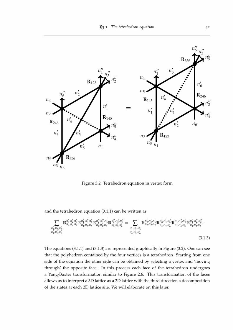
§3.1 The tetrahedron equation 41
=
R145
R123
R356
R246
n6n3
n5
n4
n2
n′′6
n1
n′′5
n′′4
n′′1 n′′3n′′2
n′3
n′4
n′1
n′2
n′5
n′6
R246
R356
R123
R145
n1n3
n2
n4
n5
n′′1
n6
n′′2
n′′4
n′′6 n′′3n′′5
n′1
n′4
n′6
n′5
n′2
n′1
Figure 3.2: Tetrahedron equation in vertex form
and the tetrahedron equation (3.1.1) can be written as
∑n′1,n′2,n′3n′4,n′5,n′6
Rn′1,n′2,n′3n1,n2,n3R
n′′1 ,n′4,n′5n′1,n4,n5
Rn′′2 ,n′′4 ,n′6n′2,n′4,n6
Rn′′3 ,n′′5 ,n′′6n′3,n′5,n′6
= ∑n′1,n′2,n′3n′4,n′5,n′6
Rn′3,n′5,n′6n3,n5,n6R
n′2,n′4,n′′6n2,n4,n′6
Rn′1,n′′4 ,n′′5n1,n′4,n′5
Rn′′1 ,n′′2 ,n′′3n′1,n′2,n′3
.
(3.1.3)
The equations (3.1.1) and (3.1.3) are represented graphically in Figure (3.2). One can seethat the polyhedron contained by the four vertices is a tetrahedron. Starting from oneside of the equation the other side can be obtained by selecting a vertex and ’movingthrough’ the opposite face. In this process each face of the tetrahedron undergoesa Yang-Baxter transformation similar to Figure 2.6. This transformation of the facesallows us to interpret a 3D lattice as a 2D lattice with the third direction a decompositionof the states at each 2D lattice site. We will elaborate on this later.

42 A 3D Integrable Model
=
Lα,γ
Lα,β
R123
Lβ,γ
n4
n2
n1
n′′4
n′′1n′′2
n′4
n′1
n′2 Lβ,γ
R123
Lα,β
Lα,γ
n1
n2
n4
n′′1
n′′2
n′′4
n′4
n′2
n′1
Figure 3.3: Tetrahedron RLLL relation
3.2 A solution with positive Boltzmann weights
In this section we review a solution to the tetrahedron equation originally found byBazhanov, Mangazeev and Sergeev. The method involves the use of a functional formof the tetrahedron equation [7] whereby we consider the action of the map R123 on theq-oscillator algebra and under extra assumptions construct representations of it.
Just like in the 2D case where we considered a generalised RLL-Yang Baxter equa-tion (2.4.4) represented graphically in Figure 2.7, we consider a generalised RLLL-tetrahedron equation of the form
Lα,βLα,γLβ,γR123 = R123Lβ,γLα,γLα,β (3.2.1)
illustrated in Figure 3.3. These L-operators are different to those used in (2.4.4). ThereR was already given explicitly and the remaining space was left as a representationspace of L-operator algebra (2.4.7). In this case R is not known and we will consider
§3.2 A solution with positive Boltzmann weights 43
the space it acts in(white lines in Figure 3.3) abstractly with (3.3) determining relationsbetween the operators from each vertex. The tetrahedron equation (3.2) ensures thatthe L-operator algebra determined by (3.3) is associative.
For the solution constructed in this chapter we will consider an algebra constructedfrom a q-oscillator algebra placed at each vertex L.
3.2.1 q-oscillator algebra and Fock space representations
Definition 3.2.0.1 (q-oscillator algebra Oscq). The q-oscillator algebra is generated byk, a+, a− over C(q, q−1) subject to the relations
ka± = q±1a±k, qa+a− − q−1a−a+ = q− q−1, (3.2.2a)
k2 = q(1− a+a−) = q−1(1− a−a+). (3.2.2b)
The q-oscillator algebra is a ‘building block’ of the solution to the tetrahedron equationwe construct in this section. Therefore we also need to consider its representations. Inparticular, we will consider the infinite-dimensional irreducible anti-Fock space repre-sentation F−q spanned by |n〉n∈Z≥0 with scalar product
〈m|n〉 = δn,m, N |n〉 = n |n〉 , 〈n|N = 〈n| n (3.2.3)
where N is the occupation number operator. The q-oscillator algebra action on this spaceis given by
k = q−N−1/2, (3.2.4a)
a+ |0〉 = 0, a− |n〉 = |n + 1〉 , a+ |n〉 = (1− q−2n) |n− 1〉 , (3.2.4b)
〈0| a− = 0, 〈n| a− = 〈n− 1| , 〈n| a− = 〈n + 1| (1− q−2−2n). (3.2.4c)
It is called the anti-Fock space representation because a+ annihilates the vacuum state|0〉. In the next section we use this representation to construct a solution to (3.1.1).

44 A 3D Integrable Model
3.2.2 Functional Tetrahedron equation
The remaining spaces (denoted as black lines in Figure 3.3) are identified with C2. Inparticular, we choose L [9] as
L(k, a±) =
1 0 0 00 k a+ 00 a− −k 00 0 0 1
, (3.2.5)
acting in C2 ⊗C2 with operator valued entries. Entries in (3.2.5) are indexed such thatthe indices for the second space index 2× 2 blocks while indices for the first space indexthe entries in each block. In (3.3) we label these two-dimensional spaces by α, β and γ
and label the L operators appropriately.
Now we define the map R123 : Oscq ⊗Oscq ⊗Oscq → Oscq ⊗Oscq ⊗Oscq by the innerautomorphism
R123(x) = R123xR−1123 ∀x ∈ Oscq ⊗Oscq ⊗Oscq, (3.2.6)
R123(a±i ) = a′±i , R123(ki) = k′i, i = 1, 2, 3. (3.2.7)
Then we can rewrite (3.2.1) as
Lα,β(k1, a±1 )Lα,γ(k2, a±2 )Lβ,γ(k3, a±3 ) = R123(
Lβ,γ(k3, a±3 )Lα,γ(k2, a±2 )Lα,β(k1, a±1 ))
= Lβ,γ(k′3, a′±3 )Lα,γ(k′2, a′±2 )Lα,β(k′1, a′±1 ). (3.2.8)
Substituting (3.2.5) into (3.2.8) we find that R123 is determined by the relations
k′2a′±1 = k3a±1 + k1a±2 a∓3 , (3.2.9a)
a′±2 = a±1 a±3 + k1k3a±2 , (3.2.9b)
k′2a′±3 = k1a±3 + k3a∓1 a∓2 , (3.2.9c)
k′1k′2 = k1k2, k′2k′3 = k2k3, (3.2.9d)(k′2)2
= k21k2
2k23 + k1k3
(q−1a+
1 a−2 a+3 + qa−1 a+
2 a−3)
+ k21 + k2
3 − (q + q−1)k21k2
3. (3.2.9e)

§3.2 A solution with positive Boltzmann weights 45
Applying the representation (3.2.4) to the these relations one can determine recurrencerelations for R
n′1,n′2,n′3n1,n2,n3 using (3.2.6), (3.2.7) and (3.1.2). Doing so we find
Rn′1,n′2,n′3n1,n2,n3 = δn1+n2,n′1+n′2
δn2+n3,n′2+n′3
qn2(n2+1)−(n2−n′1)(n2−n′3)
(q2; q2)n2
Qn2(x, y, z) (3.2.10)
where x = q−2n′1 , y = q−2n′2 , z = q−2n′3 and
Qn+1(x, y, z) = (x− 1)(z− 1)Qn(xq2, y, zq2) + xz(y− 1)q2nQn(x, yq2, z), (3.2.11)
Q0(x, y, z) = Q0(xq−2, y, z) = Q0(x, yq−2, z) = Q0(x, y, zq−2) (3.2.12)
Choosing the normalisation R0,0,00,0,0 = 1, equation (3.2.12) allows us to set Q0(x, y, z) =
1 ∀x, y, z ∈ q−2nn∈Z≥0 . Using this to solve the recurrence relation (3.2.11) we find R
to be
Rn′1,n′2,n′3n1,n2,n3 = δn1+n2,n′1+n′2
δn2+n3,n′2+n′3q−n2(1+n1+n3)−n′1n′3
×[
n1 + n2
n1
]q2
2φ1
(q−2n2 q−2n′1
q−2n1−2n2
∣∣∣∣∣ q2, q2(1+n′3)
), (3.2.13)
solving (3.1.3) by construction. We shall refer to this matrix representation of the oper-ator R as the 3D R-matrix. The formula contains q-binomials defined in (B.1.4) and aterminating basic hypergeometric series as defined in (B.1.9). We will use this notationregularly throughout the rest of the thesis.
We also notice that due to conservation laws we always have n2 ≤ n1 + n2 and n′1 ≤n1 + n2. As a result, for summands with a sufficiently large index, the numerator yieldsa double zero and the series terminates despite a simple zero in the denominator. In ad-dition, the hypergeometric function in (3.2.13) does not require a regularisation and therange of the summation can be taken to be from 0 to min(n2, n′1). All nonzero elementsin (3.2.13) are positive for 0 < q < 1 as explained in [9] where it was first introduced.
The R-Matrix (3.2.13) possesses a number of symmetries which are generated by twoelementary ones
Rn′1,n′2,n′3n1,n2,n3 = R
n′3,n′2,n′1n3,n2,n1 , R
n′1,n′2,n′3n1,n2,n3 = qn3−n2+n2
1−n′21(q2; q2)n′1(q2; q2)n1
Rn1,n′3,n′2n′1,n3,n2
. (3.2.14)

46 A 3D Integrable Model
They can be proved by using Heine’s transformations (B.2.6) for φ2 1 series . We list heretwo other useful symmetries which follow from (3.2.14):
Rn′1,n′2,n′3n1,n2,n3 = qn1−n2+n2
3−n′23(q2; q2)n′3(q2; q2)n3
Rn′2,n′1,n3
n2,n1,n′3(3.2.15)
and
Rn′1,n′2,n′3n1,n2,n3 = q(n3+n′3+2n′1−2n2+1)(n1−n′1)
3
∏i=1
(q2; q2)n′i(q2; q2)ni
Rn1,n2,n3n′1,n′2,n′3
. (3.2.16)
Let us notice that up to the factor q−n2(1+n1+n3)−n′1n′3 the expression (3.2.13) is a poly-nomial in q2n′3 and can be formally continued to negative values n3, n′3 < 0. So let usassume that ni, n′i ≥ 0, i = 1, 2 and n3, n′3 ∈ Z provided that all indices are still con-strained by delta-functions entering (3.2.13). Then it is easy to find a transformation ofmatrix elements of the 3D R-matrix under the replacement q→ q−1
Rn′1,n′2,n′3n1,n2,n3
∣∣∣q→q−1
= q(n1−n′2)(n2−n′2−1)Rn′1,n′2,−n3−1n1,n2,−n′3−1. (3.2.17)
Extra parameters can be added to (3.2.13) without affecting the equality of (3.1.3). Inparticular, the function
[R(λ, µ, c)]n′1,n′2,n′3
n1,n2,n3= cn′1−n1
1 cn′2−n22 cn′3−n3
3
(µ3
λ1
)n2(
λ2
λ3
)n′1(
µ1
µ2
)n′3R
n′1,n′2,n′3n1,n2,n3 (3.2.18)
for triples λ = λ1, λ2, λ3, µ = µ1, µ2, µ3 and c = c1, c2, c3. The factors dependingon c is just a diagonal similarity transform and it drops out of the tetrahedron trivially.The factors in µ, λ is also fairly easy to show; using the two delta functions at each ver-tex in (3.1.3) one can move all factors in µ, λ on the internal edges to the external edges.Comparing the external edges of both sides of the equation shows they are equal andhence the tetrahedron equation is not affected.
We will refer (3.2.18) as a ‘dressed’ 3D R-Matrix. These factors are important in the con-struction of certain objects of interest such as the layer-to-layer transfer matrix wherethey allow one to introduce two spectral parameters and thereby an infinite family ofcommuting operators for this 3D model. It also allows us to introduce a spectral pa-rameter to a 2D R-matrix whose construction we will consider in the next section. ThisR-matrix related to Uq(sln) and using (3.2.18) we will give a new presentation for itsmatrix elements.
§3.3 n-layer projection 47
3.3 n-layer projection
We consider a ‘composite weight’ S constructed from the dressed R-Matrix (3.2.18) bymultplying n copies of it together in the third space and taking the trace. That is
Si′,j′
i,j := ∑k
n
∏s=1
[R(λs, µs, cs)]j′s,i′s,ks+1js,is,ks
(3.3.1)
where kn+1 = k1, λs = (λ1,s, λ2,s, λ3,s) and similarly for µs, cs. We note that the deltafunctions contained in each factor (3.2.13) imply the global conservation laws
I = I′, J = J′, (3.3.2)
I :=n
∑s=1
is, I′ :=n
∑s=1
i′s, J :=n
∑s=1
js, J′ :=n
∑s=1
j′s. (3.3.3)
We now consider the case where λ3,s and µ3,s are equal for all s. Using these conserva-tion laws for the indices we can rewrite S as
S(w, Φ, Ψ)i′,j′
i,j = Φh(i)Φv(j′)Ψh(i, i′)Ψv(i, i′)∑k
wk1n
∏s=1
Rj′s,i′s,ks+1js,is,ks
(3.3.4)
where
w =n
∏s=1
µ1,s
µ2,s(3.3.5a)
Φh(i) =n−1
∏s=1
φikh,k, Φv(j′) =
n−1
∏s=1
φj′kv,k, (3.3.5b)
Ψh(i, i′) =n−1
∏s=1
ψi′k−ikh,k , Ψv(i, i′) =
n−1
∏s=1
ψj′k−jkv,k , (3.3.5c)
φh,k =λ1,n
λ1,k, φv,k =
λ2,k
λ1,n, (3.3.5d)
ψh,k =c2,k
c2,n
n−1
∏s=k
µ1,s
µ2,s, ψv,k =
c1,kλ2,k
c1,nλ1,n. (3.3.5e)
Here we have also removed any factors in (3.3.1) depending solely on I, J because theyare constants. The tetrahedron equation implies that this composite weight satisfies theYang-Baxter equation
∑i′,j′k′
Si′,j′
i,j (w, Φ, Ψ)Si′′,k′i′,k (w′, Φ
′, Ψ
′)S
j′′,k′′
j′,k′ (w′/w, Φ
′′, Ψ
′′) = (3.3.6)

48 A 3D Integrable Model
∑i′,j′k′
Sj′,k′
j,k (w′/w, Φ′′, Ψ
′′)Si′,k′′
i,k′ (w′, Φ
′, Ψ
′)S
i′′,j′′
i′,j′ (w, Φ, Ψ)
provided that the functions Φ, Ψ, Φ′, Ψ
′, Φ
′′, Ψ
′′ are constrained by the relations
φv,k = φ′v,k, φ
′h,k = φ
′′h,k, φ
′′v,k = φ−1
h,k , ψ′′v,k =
ψh,kψ′v,kψ
′′h,k
φh,kψv,kψ′h,k
∀k = 1, . . . n− 1. (3.3.7)
These constraints are again a consequence of the delta functions appearing in (3.2.13).It is clear from (3.3.6) that S(w) is a R-matrix with the parameter w in (3.3.4) playing therole of the spectral parameter. The other parameters Φ, Ψ and their constraints (3.3.7)give us some freedom in writing down the R-matrix. Their dependence on indicesi, j, i′, j′ are rather simple - the Ψ are gauge transformations of the R-matrix while theΦ are ’fields’ in the physical sense which affect the Boltzmann weights of the underly-ing model.
The functions Φ, Ψ do play a nontrivial role when considering the transfer matrix builtfrom S(w) as in (2.3.27) where they can affect the spectrum and commutativity if notchosen carefully. Since we are currently interested in the R-Matrix and not the globalproperties of the model, for now we can set these functions to 1 without loss of gener-ality.
The R-Matrix S(w) is composite in the sense that it is a direct sum of “smaller” R-matrices. It is a fact which follows from considering the conservation laws (3.3.2) ap-plied to each component in (3.3.6). By fixing the external indices in equation (3.3.6),it can be observed that the equation reduces to a tensor sum of an infinite number ofthe Yang-Baxter equations on subspaces indexed by global parameters I, J, K = 0, . . . , ∞defined in (3.3.3).
In particular, it was argued in [7; 9] that the subspace for each parameter I is in factthe underlying space of the rank I symmetric tensor representation of Uq(sln) and theaction of S on this space is the corresponding R-matrix
Si′,j′
i,j (w) =∞⊕
I,J=0
R(n)I,J (w). (3.3.8)
The case n = 2 in (3.3.4) was considered in [10] which resulted in a new formula for thematrix elements of the R-Matrix for Uq(sl2) acting in the tensor product of representa-tions of highest weight I and J. Setting I = J = 1 the formula gives the R-matrix for

§3.3 n-layer projection 49
S(w)i′,j′
i,j =
i1
j1
i′1
j′1
k1
k2
i2
j2
i′2
j′2
k3
iN
jN
i′N
j′N
kN−1
Figure 3.4: n-layer projection of the 3-dimensional model
the 6-vertex model.
The R-matrices R(n)I,J (w) in (3.3.8) are irreducible and now we will give a new pre-
sentation for them by extracting a formula for them from the expression (3.3.1). Firstlet us introduce some vector notations. We denote by i := i1, . . . , ir a vector with rcomponents ik ∈ Z≥0 and define
|i| =r
∑s=1
is, (i, j) =r
∑s=1
is js. (3.3.9)
Addition is done component-wise and we introduce two permutations σ and τ actingon k as
σk1, . . . , kr = k2, . . . , kr, k1, (3.3.10)
τk1, . . . , kr = kr, kr−1, . . . , k1 (3.3.11)
of the vector coordinates. The dimension r can take values n and n − 1 as explainedbelow.

50 A 3D Integrable Model
The Kronecker delta function of two vectors is zero unless all their components match,i.e.
δi,j =r
∏s=1
δis,js . (3.3.12)
We also note that in discussing S(w) and R(n)I,J (w) the vectors i, j, i′, j′ have different
dimensions. When we use S(w), the n-layer composite weight, it is implied that the di-mension r = n. When we derive the expression for the R-Matrix R(n)
I,J , it is implied thatthe dimension r = n− 1 because by fixing I, J the relation (3.3.3) implies that we canremove one of the indices. Typically we choose to remove last components in, jn, i′n, j′nand replace them with I − |i|, J − |j| etc. except in certain cases where it is more con-venient to keep them. Of course, in evaluating final expressions the replacement has tobe made regardless.
Combining (3.2.13) and (3.3.4) the composite weight Si′,j′
i,j (w) can be written as
Si′,j′
i,j (w) = δi+j,i′+j′ ∑k∈Zn
≥0
δi+k,i′+σk wk1 q−|i|−(i,j)−(k,i+σ−1 j′)n
∏s=1
[is + js
is
]q2
(3.3.13)
× ∑m∈Zn
≥0
n
∏s=1
(q−2is , q−2j′s ; q2)ms
(q2, q−2is−2js ; q2)ms
q2|m|+2(m,σk).
The above formula contains 2n summations. The n summations in k are non-terminating.The n summations in m are restricted by 0 ≤ ms ≤ min(is, j′s), s = 1, . . . , n due to thepresence of Pochhammer symbols in the numerator. Let us also notice that all sumsin m′s terminates before the Pochhammer symbols in the denominator become zero.Therefore, there is no need for a regularisation.
This formula is quite easy to simplify. The presence of delta functions in (3.3.13) leadto the following global conservation laws for the spin indices i, j, i′, j′,
i1 + · · ·+ in = i′1 + · · ·+ i′n = I, j1 + · · ·+ jn = j′1 + · · ·+ j′n = J (3.3.14)
which allows us to remove one of the indices from i, j, i′, j′ once we fix integers I, J.Furthermore, we can also express k2, . . . , kn in terms of k1 by the relations
ks+1 = ks + is − i′s, kn = k1 +n−1
∑s=1
(is − i′s), (3.3.15)
which allows us to rewrite the sum in k as a single sum in k1. However, some care mustbe taken in computing this sum. Note that when i′s > is for some s, the summation

§3.3 n-layer projection 51
range of ks implies contributions to the sum for negative values of ks+1 not included inthe expression (3.3.13). These contributions turn out to be trivial. To see that we firstnotice that
Rn′1,n′2,n′3n1,n2,n3 = 0, n3 < 0, n′3 ≥ 0 (3.3.16)
This follows from (3.2.15) since the factor 1/(q2; q2)n3 becomes zero and all other factorsare nonzero. Now let us look at the product in (3.3.4) and assume that there are contri-butions from negative values for some ks, s = 1, . . . , n. All ks cannot be negative, sincek1 ≥ 0. Since the product is cyclic, we will always find at least one factor R
j′s,i′s,ks+1js,is,ks
suchthat ks < 0 and ks+1 ≥ 0. This factor will be equal to zero because of (3.3.16). Therefore,all factors which contain some negative ks automatically disappear and we can safelysum over k1 from 0 to ∞ in (3.3.13) with substitutions (3.3.15). As one can easily see thesum on k1 becomes a geometric series which converges provided
wq−I−J < 1, 0 < q < 1. (3.3.17)
Once this condition is satisfied for w = λ2 > 0, the sum in (3.3.4) has only positiveterms, since all matrix elements of the 3D R-matrix (3.2.13) are positive. Restrictingthe result to fixed positive values I, J we get the expression for matrix elements of theoperator R(n)
I,J (w) in (3.3.8). The result reads
[R(n)
I,J (λ)]i′,j′
i,j= δi+j,i′+j′ qΨ
n
∏s=1
[is + js
is
]q2
∑m∈Zn
≥0
q2|m|+2 ∑
k≥lmk(il−i′l)
1− λ2q2|m|−I−J
n
∏s=1
(q−2is , q−2j′s ; q2)ms
(q2, q−2(is+js); q2)ms
(3.3.18)
where
Ψ = −2(i, j) + (i′, j′)− (I − |i|)(J − |j|) + I(|i′| − |i| − 1) + ∑1≤k<l≤n−1
(i′k j′l − ik jl).
(3.3.19)Here in the left-hand side of (3.3.18) and in the expression for the phase factor (3.3.19)we used (n− 1)-component indices, see (3.3.9) with r = n− 1. However, in the right-hand side of (3.3.18) for compactness we kept n-component external indices assumingthat we need to substitute in, jn, i′n, j′n from (3.3.14). The formula has n summationindices m1, m2, . . . , mn which terminates after finitely many terms. Finally we noticethat the sum ∑k≥l in (3.3.18) taken over n ≥ k ≥ l ≥ 1 can be restricted to the valuesn− 1 ≥ k ≥ l ≥ 1, since it is equal to zero for k = n due to (3.3.14).

52 A 3D Integrable Model
The case n = 2 of (3.3.18) was given in equation (75) of [9]. This formula generateselements of a (I+n−1
n−1 )× (J+n−1n−1 )-dimensional matrix determined by indices 0 ≤ |i|, |i′| ≤
I, 0 ≤ |j|, |j′| ≤ J.
As the next step we shall evaluate one sum in (3.3.18) and reduce the total numberof summations to n− 1. We use the same method as in [10].
We start with the Lagrange interpolating formula
k
∑l=0
xx− ql
ql(q−k; q)l
(q; q)lPk(ql) =
Pk(x)(q; q)k
xk(x−1; q)k+1, (3.3.20)
which is valid for any polynomial Pk(x) of degree at most k. First we define a newvariable
l = m1 + · · ·+ mn (3.3.21)
which runs from 0 to I and use l instead of mn. Then one can rewrite (3.3.18) as
[R(n)
I,J (λ)]i′,j′
i,j= δi+j,i′+j′(−1)|i|−|i
′|q−2(i,j)+(i′,j′)−(I−|i|)(J−|j|)+I(|i′|−|i|−1)+∑k<l(i′k j′l−ik jl)
×q(|i|−|i
′|)(|j|+|j′|−2J−1)(q−2J ; q2)|j|(q−2J ; q2)|j′|(q2; q2)I
n−1
∏s=1
[is + js
is
] I
∑l=0
q2l
1− λ2q−I−J+2l(q−2I ; q2)l
(q2; q2)lPI(q2l).
(3.3.22)
The summation in l matches (3.3.20) with k = I, x = λ−2qI+J and
PI(q2l) = q2l(I+|i|−|i′|) ∑m
q2(|m|+∑l>k mk(i′l−il))n−1
∏s=1
(q−2is , q−2j′s ; q2)ms
(q2, q−2(is+js); q2)ms
(3.3.23)
× (q−2l ; q2)|m|(q2(1−l+J−|j′|+|m|; q2)I−|i′|(q
2(1−l+I−|i|+|m|); q2)|i|−|m|.
The polynomial PI(x) in (3.3.23) has degree of at most I and therefore we can replacethe sum in l in (3.3.22) with the right hand side of (3.3.20) to find the expression
Proposition 3.3.1.
[R(n)
I,J (λ)]i′,j′
i,j= δi+j,i′+j′
[A(n)
I,J (λ)]i′,j′
i,jBI,J(λ) q
(i′,j′)−(i,j)−J|i|−I|j′|+ ∑k>l
(ik jl+j′ki′l)(3.3.24)
× ∑m∈Zn−1
≥0
(λ2q−I−J , λ2q2+I+J−2|i|−2|j|; q2)|m|
(λ2q2+I−J−2|i|, λ2q2+J−I−2|j′|; q2)|m|
n−1
∏s=1
(q−2is , q−2j′s ; q2)ms
(q2, q−2(is+js); q2)ms
q2(|m|+ ∑
k<lmk(i′l−il))
.

§3.3 n-layer projection 53
All external and summation indices in (3.3.24) have n− 1 components and the coeffi-cients A(n)
I,J (λ)i′,j′
i,j and BI,J(λ) are given by
[A(n)
I,J (λ)]i′,j′
i,j=
(λ−2qI−J ; q2)|j′|(λ−2qJ−I ; q2)|i|(q−2J ; q2)|j|
(λ−2q−I−J ; q2)|i+j|(q−2J ; q2)|j′|
n−1
∏s=1
[is + js
js
]q2
, (3.3.25)
BI,J(λ) = q−I−I J (λ2q−I−J ; q2)I+J+1
(λ2q−I−J ; q2)I+1(λ2q−I−J ; q2)J+1. (3.3.26)
The formula (3.3.24) provides an expression for the matrix elements of the Uq(sln) R-Matrix acting on the space VI ⊗VJ where
VI ≡ |i〉, |i| ≤ I. (3.3.27)
It follows from the tetrahedron equation for the 3D R-matrix (3.2.13) that (3.3.24) satis-fies the Yang-Baxter equation
R(n)I,J (λ)R(n)
I,K(λµ)R(n)J,K(µ) = R(n)
J,K(µ)R(n)I,K(λµ)R(n)
I,J (λ) (3.3.28)
for any I, J, K ∈ Z+. However, one will notice that the coefficient BI,J(λ) is just aconstant not depending on indices. We find it convenient to set this factor to 1. Inwhat follows, we will use (3.3.24) with BI,J(λ) = 1 unless stated otherwise. In thisnormalization we have [
R(n)I,J (λ)
]0,0
0,0= 1. (3.3.29)
The main reason we do this is because (3.3.24) is now well defined even when I, J ∈ C.Although the 3D model projection outlined in this paper satisfies the Yang-Baxter equa-tion for integral weights by construction, the equation (3.3.28) remains valid even forcomplex weights I, J, K ∈ C. The proof closely follows the arguments given in [20].
Consider a particular element of the Yang-Baxter equation 〈i, j, k|(3.3.28)|i′, j′, k′〉 withfixed external indices i = (i1, . . . , in−1), etc. Due to the conservation law in (3.3.24) wehave |i + j + k| = |i′ + j′ + k′| ≡ m and all summation indices in (3.3.28) will also belimited by m. Choose an integer N > m and assume that integer weights I, J, K > N. Itis easy to see that all denominators in the R-matrices entering the Yang-Baxter equationare non-zero and (3.3.28) becomes the equality of two rational functions in variablesx = q−I , y = q−J and z = q−K. After eliminating denominators we can rewrite (3.3.28)as equality of two polynomials in three variables x, y, z. The degree of these polyno-mials grows as a fixed polynomial in N. Now we know that the Yang-Baxter equation(3.3.28) is true for infinitely many integer variables I, J, K > N. It can only happen if

54 A 3D Integrable Model
(3.3.28) reduces to a polynomial identity in x, y, z ∈ C. Therefore, the Yang-Baxter equa-tion with the R-matrix (3.3.24) and normalization (3.3.29) is satisfied for I, J, K ∈ C. Inthis case it defines the infinite dimensional R-matrix corresponding to Verma modulerepresentations of Uq(sln).
To illustrate how formula (3.3.24) works, let us consider a special case n = 2. In thiscase matrix elements are indexed by indices i, j, i′, j′, and (3.3.24) becomes a single sumwhich is given by
[R(2)
I,J (λ)]i′,j′
i,j= δi+j,i′+j′qi′ j′−ij−i J−I j′
[i + j
i
]q2
(λ−2qI−J ; q2)j′(λ−2qJ−I ; q2)i(q−2J ; q2)j
(λ−2q−I−J ; q2)i+j(q−2J ; q2)j′
× 4φ3
(q−2i q−2j′ λ2q−I−J λ2q2+I+J−2i−2j
q−2i−2j λ2q2+I−J−2i λ2q2+J−I−2j′
∣∣∣∣∣ q2, q2
). (3.3.30)
This is a balanced and terminating φ4 3 basic hypergeometric series for the elementsof the Uq(sl2) R-matrix. This case was already studied in [10] and the formula giventhere is of the same type as (3.3.30) but with different arguments. Most notably, thehypergeometric sum in [10] is a polynomial in the spectral parameter λ while (3.3.30)is a rational function.
Using Sears’ transform (B.2.14) we can transform the sum in (3.3.30) to equation (5.8)in [10] by identifying
n = i, a = q−2j′ , b = λ2q−I−J , c = λ2q2+I+J−2i−2j,
d = λ2q2+I−J−2i, e = q−2i−2j, f = λ2q2+J−I−2j′ .
Let us note that (5.8) in [10] requires a regularisation but the expression (3.3.30) is freefrom any divergences.
One problem with (3.3.24) is that the hypergeometric sum is a rational function inλ. For integer I the whole expression (3.3.24) is a polynomial in λ up to an overall fac-tor (λ2q−I−J ; q2)I+1. However, when both weights I, J are non-integral, this factor is nolonger a polynomial in λ and no polynomial normalization exists. In this case we canadopt the normalization (3.3.29) where elements of the R-matrix are rational functionsof λ.
As mentioned before, using Sears’ transformation the hypergeometric sum in (3.3.24)for n = 2 can be transformed into a hypergeometric polynomial in λ up to simple q-

§3.4 Symmetries and special cases 55
binomial factors. We are aware of the An multivariable generalizations of Sears’ trans-formation in the literature, but they do not appear to be applicable to our expression forn ≥ 3. Focusing on each summation index in (3.3.24) one can easily see that it is a 4φ3
basic hypergeometric series but it is not balanced and only one of the hypergeometricseries has a q2 argument so the A1 Sears’ transformations does not apply.
We expect that a formula with a hypergeometric sum being a polynomial in λ stillexists but it probably requires a new yet to be discovered identity for multivariablehypergeometric series.
3.4 Symmetries and special cases
In this section we discuss symmetries of the R-matrix R(n)I,J (λ) given by (3.3.24). They
can be derived from the corresponding symmetries of the 3D R-Matrix generated by(3.2.14). It is actually more convenient to use (3.2.15-3.2.16) since we need to to keepa position of the third “hidden” direction where we take the trace. Applying thesetransformations to the factors in (3.3.4) we find two symmetries
[R(n)
I,J (λ)]i′,j′
i,j= λ2(|i′|−|i|)
[R(n)
J,I (λ)]τj′,τi′
τj,τi, (3.4.1)[
R(n)I,J (λ)
]i′,j′
i,j= q2[i′,j′]−2[i,j]λ2(|i′|−|i|)
n
∏s=1
(q2; q2)i′s(q2; q2)j′s
(q2; q2)is(q2; q2)js
[R(n)
I,J (λ)]τi,τj
τi′,τj′. (3.4.2)
Let us explain some notations here. In the previous section we mentioned that for theR-matrix R(n)
I,J (λ) we are using n− 1-component indices, i.e. i = i1, . . . , in−1 with thelast n-th component in = I − |i| removed and similar for j’s. However, in (3.4.2) theproduct in the right-hand side is taken over s = 1, . . . , n where for s = n we substitutethe last component as above, i.e. in = I − |i|, jn = J − |j|, etc. The transformation τ isdefined in (3.3.10).
In addition, in (3.4.2) we used a notation [i, j] for a convolution of n-component in-dices, i.e.
[i, j] = (i, j) + (I − |i|)(J − |j|). (3.4.3)
There is also a symmetry of the R-matrix which corresponds the the cyclic permutationof the n 3D R-matrices in the “hidden” direction. Let us introduce the notation
ı = I − |i|, i1, . . . , in−2, (3.4.4)

56 A 3D Integrable Model
which is equivalent to the permutation σ−1i for the n-tuple i but with the last compo-nent removed. Here we assume that I, J ∈ Z+. Performing a cyclic shift in (3.3.4) weeasily obtain [
R(n)I,J (λ)
]i′,j′
i,j= λ2(|i′|−|i|)
[R(n)
I,J (λ)]ı′,′
ı,. (3.4.5)
For example, when n = 2 this corresponds to i→ I − i and similarly for other indices.
The last symmetry follows from the transformation of the 3D R-matrix (3.2.17). Af-ter simple calculations one can obtain the following result
[R(n)
I,J (λ, q)]i′,j′
i,j= q[i,j]−[i
′,j′][
R(n)J,I (λ
−1, q−1)]j′,i′
j,i. (3.4.6)
Finally, when I = J and λ = 1 the R-matrix reduces to permutation operator
R(n)I,I (1) = P1,2 (3.4.7)
which can be seen from (3.5.2) in the next section.
3.5 Reductions and factorization
There are two special points in the spectral parameter λ = q±(I−J)/2 where the multi-ple sum in (3.3.24) reduces to one non-zero summand. These specializations producethe R-matrix without difference property with weights I, J playing the role of spectralparameters. With the normalization (3.3.29) we can choose I, J ∈ C and obtain the R-matrix acting in the tensor product of two Verma modules.
For the case of the Uq(sl2) algebra the importance of such reductions was first no-ticed in [22]. Under the choice λ = q(J−I)/2 the Uq(sl2) R-matrix of [10] reduces to theR-matrix of the Povolotsky model [61] which satisfies a stochasticity condition and de-fines a family of zero-range chipping models. A generalization of the Povolotsky modelto arbitrary rank n− 1 was obtained in the recent paper [20].
So let us start with the case λ = q(I−J)/2, I − J ∈ Z+. The expression for the R-matrix(3.3.24) contains the factor (λ−2qI−J ; q2)|j′| outside the sum which has the argument 1after the above substitution. This factor is always zero for |j′| > 0 unless it is canceledby the factor (λ2q2+J−I−|j′|; q2)|m| inside the sum. It can only happen when |m| = |j′| orm = j′, since ms ≤ j′s, s = 1, . . . , n− 1. Let us note that the argument fails when J − I is

§3.5 Reductions and factorization 57
a positive integer because the other factor in the denominator can cancel with the zeroof (λ−2qI−J ; q2)|j′| and multiple summands survive.
After simple algebra one can derive from (3.3.24) the following result
[R(n)
I,J (qI−J
2 )]i′,j′
i,j= δi+j,i′+j′q
(i′,j′)−(i,j)−J|i|−I|j′|+2J|j′|+ ∑k>l
(ik jl+j′ki′l−2j′k jl)
×(q−2J ; q2)|j|(q2J−2I ; q2)|i′|−|j|
(q−2I ; q2)|i′|
n−1
∏s=1
[i′sjs
]q2
. (3.5.1)
Similarly, we can make the substitution λ = qJ−I
2 for J − I ∈ Z+. In this case theargument is the same except with the factors (λ−2qJ−I ; q2)|i| and (λ2q2+I−J−|i|; q2)|m|and so the only summand that contributes is m = i. Then we obtain
[R(n)
I,J (qJ−I
2 )]i′,j′
i,j= δi+j,i′+j′q(i
′,j′)−(i,j)−J|i|−I|j′|+2I|i|+∑k>l(ik jl+j′ki′l−2iki′l)
×(q−2I ; q2)|i|(q2I−2J ; q2)|j′|−|i|
(q−2J ; q2)|j′|
n−1
∏s=1
[j′sis
]q2
. (3.5.2)
Obviously these reductions are substantially simpler than the original R-matrix. Asmentioned above I, J play role of the spectral parameters for these R-matrices and cannow take arbitrary complex values.
In fact, one can construct the full R-matrix as a matrix product of (3.5.1)-(3.5.2). Toexplain this it is convenient to apply a simple similarity transformation in the firstspace and introduce
R(n)I,J (λ) = U ⊗ 1 R(n)
I,J (λ) U−1 ⊗ 1 (3.5.3)
withUi,i′ = δi,i′
(λq(I−J)/2
)|i|. (3.5.4)
We now define two operators M and N acting in the tensor product of two Vermamodules by
M(qI , qJ) = R(n)I,J (q
I−J2 ), N(qI , qJ) = R(n)
I,J (qJ−I
2 ) (3.5.5)
where as usual R1,2(λ) = P1,2R1,2(λ), etc. with P1,2 being the permutation operator.Both operators M(qI , qJ) and N(qI , qJ) of complex arguments qI , qJ are defined by itsmatrix elements via (3.5.1)-(3.5.2) and (3.5.5).
With these notations one can easily derive from (3.3.24) the following factorization

58 A 3D Integrable Model
Proposition 3.5.1.
R(n)I,J (λ) = M(λq
I+J2 , qJ)N(λ−1q
I+J2 , qJ). (3.5.6)
A similar factorization of the R-matrix appeared in [25] for the sl2 case of the XXXmodel.
We can also rewrite a factorization formula (3.5.6) for the matrix elements of the originalR-matrix R(n)
I,J (λ) as follows
[R(n)
I,J (λ)]i′,j′
i,j= ∑
k+l=i+jMk,l
i,j Ni′,j′
k,l , (3.5.7)
with
Mi′,j′
i,j = δi+j,i′+j′ q−J|i|−(i,j)+ ∑
k>l(ik jl+j′ki′l−2j′k jl) (q−2J ; q2)|j|(λ
−2qJ−I ; q2)|i′−j|
(λ2q−I−J)|j′|(λ−2q−I−J ; q2)|i′|
n−1
∏s=1
[i′sjs
]q2
,
(3.5.8a)
Ni′,j′
i,j = δi+j,i′+j′ q(i′,j′)−I|j′|+ ∑
k>l(jkil+j′ki′l−2jki′l) (λ
2q−I−J ; q2)|j|(λ−2qI−J ; q2)|j′−j|
(q−2J ; q2)|j′|
n−1
∏s=1
[j′sjs
]q2
(3.5.8b)
where we removed some gauge factors which cancel in the matrix product (3.5.7).
3.6 Comparison with other results
In this and next sections we will compare (3.3.24) with some other presentations of theUq(sln) related R-matrix given in the literature. We will establish a connection with thestandard the Uq(sln) L-operator presented in [20] and also compare our results withsome higher-spin examples of the Uq(sl3) R-Matrix.
We start with some remarks regarding the coefficient A(n)I,J (λ) in (3.3.25). For specific ele-
ments of the R-matrix the q-Pochhammer symbols are finite products as their argumentsare integers. If we want to derive the formula for the L-operator as an n× n-matrix withoperator entries acting in the Verma modules spanned by |j〉 = |j1, . . . , jn−1〉 we need torewrite (3.3.25) in the form suitable for abstract values of j indices.
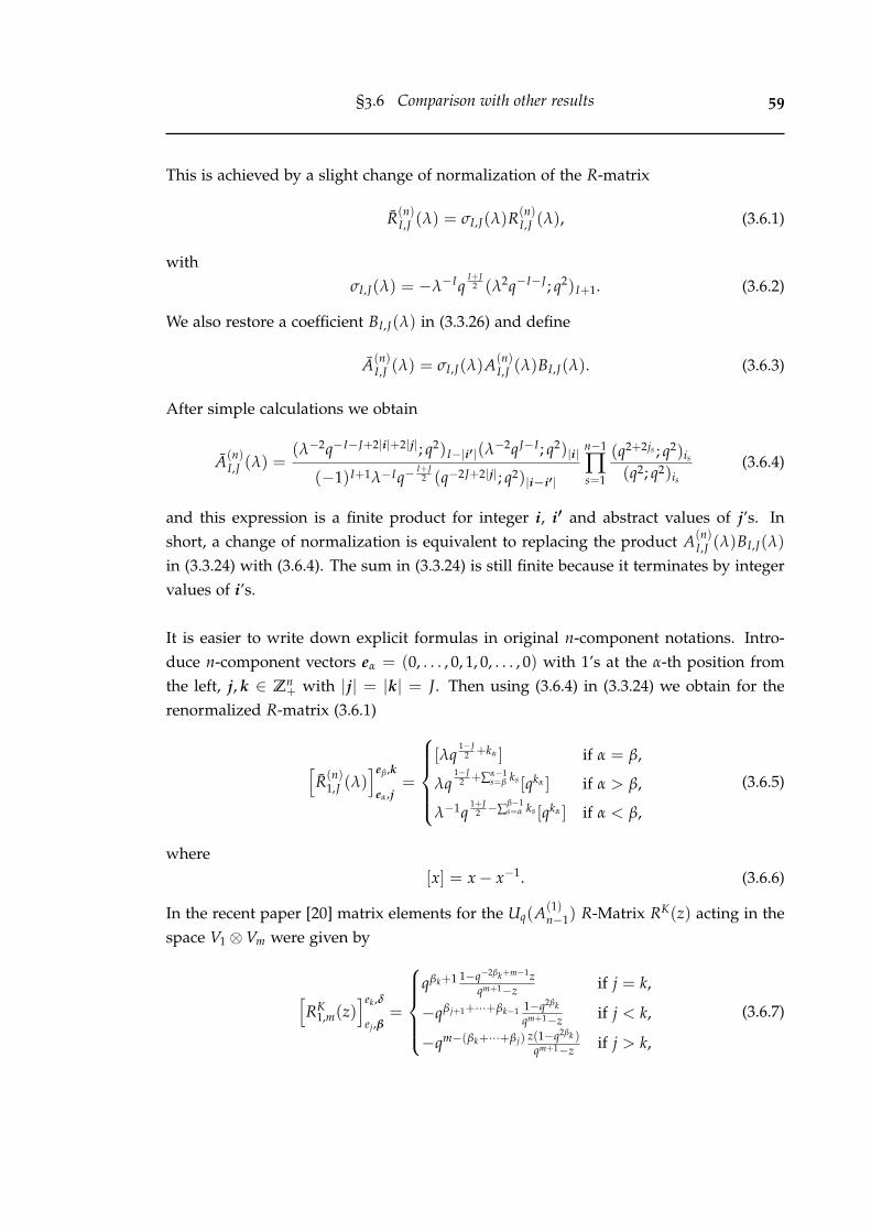
§3.6 Comparison with other results 59
This is achieved by a slight change of normalization of the R-matrix
R(n)I,J (λ) = σI,J(λ)R(n)
I,J (λ), (3.6.1)
withσI,J(λ) = −λ−Iq
I+J2 (λ2q−I−J ; q2)I+1. (3.6.2)
We also restore a coefficient BI,J(λ) in (3.3.26) and define
A(n)I,J (λ) = σI,J(λ)A(n)
I,J (λ)BI,J(λ). (3.6.3)
After simple calculations we obtain
A(n)I,J (λ) =
(λ−2q−I−J+2|i|+2|j|; q2)I−|i′|(λ−2qJ−I ; q2)|i|
(−1)I+1λ−Iq−I+J
2 (q−2J+2|j|; q2)|i−i′|
n−1
∏s=1
(q2+2js ; q2)is
(q2; q2)is
(3.6.4)
and this expression is a finite product for integer i, i′ and abstract values of j’s. Inshort, a change of normalization is equivalent to replacing the product A(n)
I,J (λ)BI,J(λ)
in (3.3.24) with (3.6.4). The sum in (3.3.24) is still finite because it terminates by integervalues of i’s.
It is easier to write down explicit formulas in original n-component notations. Intro-duce n-component vectors eα = (0, . . . , 0, 1, 0, . . . , 0) with 1’s at the α-th position fromthe left, j, k ∈ Zn
+ with |j| = |k| = J. Then using (3.6.4) in (3.3.24) we obtain for therenormalized R-matrix (3.6.1)
[R(n)
1,J (λ)]eβ,k
eα,j=
[λq
1−J2 +kα ] if α = β,
λq1−J
2 +∑α−1s=β ks [qkα ] if α > β,
λ−1q1+J
2 −∑β−1s=α ks [qkα ] if α < β,
(3.6.5)
where[x] = x− x−1. (3.6.6)
In the recent paper [20] matrix elements for the Uq(A(1)n−1) R-Matrix RK(z) acting in the
space V1 ⊗Vm were given by
[RK
1,m(z)]ek ,δ
ej,β=
qβk+1 1−q−2βk+m−1z
qm+1−z if j = k,
−qβ j+1+···+βk−1 1−q2βk
qm+1−z if j < k,
−qm−(βk+···+β j) z(1−q2βk )qm+1−z if j > k,
(3.6.7)

60 A 3D Integrable Model
and the elements of RK(z) acting on Vl ⊗V1 were given by
[RK
l,1(z)]γ,ek
α,ej=
qγk+1 1−q−2γk+l−1z
ql+1−z if j = k
−ql−(αj+···+αk) z(1−q2αk )ql+1−z if j < k,
−qαk+1+···+αj−1 1−q2αk
ql+1−z if j > k,
(3.6.8)
where we write them in the same notations as in (3.6.5).A direct comparison of (3.6.7) and (3.6.5) gives
[R(n)
1,J (λ)]eβ,k
eα,j=[λq
1+J2
]q[eβ,k]−[eα,j]
[RK
1,J(λ−2)]eα,j
eβ,k. (3.6.9)
To compare matrix elements of RKl,m(z) with our formula (3.3.24) for other cases we must
first identify their parameters. So we set l = I, m = J and z = λ−2. The normalizationof the R-matrix RK
l,m(z) is the same as (3.3.29) for R(n)I,J (λ). Therefore, we expect that for
arbitrary I, J [R(n)
I,J (λ)]i′,j′
i,j= q[i
′,j′]−[i,j][
RKI,J(λ
−2)]i,j
i′,j′. (3.6.10)
The difference between two R-matrices in (3.6.10) is easy to explain. The matrix ele-ments of R(n)
I,J (λ) are defined similar to (3.1.2), i.e.
[R(n)
I,J (λ)]i′,j′
i,j= 〈i, j|R(n)
I,J (λ)|i′, j′〉. (3.6.11)
However, the matrix elements of RKl,m(z) in [20] are defined by the transposed action
[RK
l,m(z)]γ,δ
α,β= 〈γ, δ|RK
l,m(z)|α, β〉 . (3.6.12)
It is easy to check that the extra “twist” factor q[i′,j′]−[i,j] in (3.6.10) drops out from the
Yang-Baxter equation.
We have checked that the relation (3.6.10) holds for the Uq(A(1)1 ) and Uq(A(1)
2 ) R-matrices for all cases given in Appendix A of [20].
It is also interesting to compare our reductions (3.5.1) and (3.5.2) with that obtainedin [20]. In particular, we expect that the Theorem 2 in [20]
[RK
l,m(ql−m)
]γ,δ
α,β= δα+β,γ+δqψ
[ml
]−1
q2
n+1
∏s=1
[βs
γs
]q2
, (3.6.13)

§3.6 Comparison with other results 61
ψ = ∑1≤s,t≤n+1
αs(βt − γt) + ∑1≤s,t≤n+1
(βs − γs)γt (3.6.14)
should correspond to the substitution λ = qJ−I
2 given by (3.5.2). A direct calculationshows the relation (3.6.10) also holds in this case.
Now let us turn to the Uq(sln) L-operator. When J = 1 the expression (3.6.5) fur-ther reduces to the trigonometric n-state R-Matrix [62; 63]. We shall also use a twistedversion of this R-matrix [64] which we give in the form stated in [65]
Rβ,δα,γ(λ) = δα,βδγ,δδα,γ(q− 1)(λ + λ−1q−1) + δα,βδγ,δρα,γ(λ− λ−1) + δα,δδβ,γσα,β, (3.6.15)
where
σα,β =
0 if α = β,
(q− q−1)λ if α < β,
(q− q−1)λ−1 if α > β
(3.6.16)
and ρα,β are nonzero complex parameters such that
ρα,α = ρα,βρβ,α = 1, α, β = 1, . . . , n. (3.6.17)
Setting all ρα,β = 1 and taking convention that all indices α, β, γ, δ = 1, . . . , n in (3.6.15)denote positions of 1’s counted from the right, i.e. α ≡ en−α+1 we obtain that (3.6.15) isequivalent to (3.6.5) with J = 1.
Setting I = J = 1 in the Yang-Baxter equation (3.3.28) we obtain the L-operator al-gebra
R1,2(λ/µ)L1(λ)L2(µ) = L2(µ)L1(λ)R1,2(λ/µ), (3.6.18)
where the R1,2(λ)-matrix corresponds to the standard Uq(A(1)n−1) trigonometric R-matrix
(3.6.5) with J = 1. The L-operators L(λ) are identified with R(n)1,K(λ) (3.6.5) acting in the
“quantum” space with the weight K.
To rewrite the L-operator in algebraic notations let us introduce Weil operators Xk, Zk,i = 1, . . . , n acting in the space of n-component vectors |j〉, js ∈ Z, s = 1, . . . , n and theirconjugates such that
Zk|j〉 = qjk |j〉, Xk|j1, . . . , jn〉 = |j1, . . . , jk + 1, . . . , jn〉, (3.6.19)

62 A 3D Integrable Model
〈j|Zk = qjk〈j|, 〈j1, . . . , jn|Xk = 〈j1, . . . , jk − 1, . . . , jn|. (3.6.20)
They satisfy the Weil algebra relations
ZkXl = qδk,l Xl , Zk, k, l = 1, . . . , n. (3.6.21)
We can now define the L-operator L(λ) as an n× n matrix with operator entries suchthat
〈j|Lα,β(λ)|k〉 =[
R(n)1,J (λ)
]eβ,k
eα,j. (3.6.22)
Using (3.6.19)-(3.6.21) we obtain
Lα,β(µ) =
[µZα] if α = β,
µ X−1α Xβ [Zα]
α−1∏
s=βZs if α > β,
µ−1qX−1α Xβ [Zα]
β−1∏
s=αZ−1
s if α < β,
(3.6.23)
where we defined a rescaled spectral parameter µ = λq1−J
2 and for any vector |j〉, |j| = J
Z|j〉 = q|j||j〉, Z =n
∏s=1
Zs. (3.6.24)
In fact, we can consider (3.6.23) as an operator solution of the algebra (3.6.18) since arescaling of the spectral parameter does not affect (3.6.18). The operator Z commuteswith (3.6.23) and all representations are characterised by its complex eigenvalue qJ .
3.7 Rational limit
In the chapters that follow we will consider some other approaches to constructingR-matrices. We will compare our results obtained from the 3D approach with theseother methods. Unfortunately, not all of these approaches have been developed in thequantum case and from them we can only get a result for rational R-matrices. Sothe only way we can compare the results from this chapter is to construct rational R-matrices from our formula (3.3.24). To begin the construction, let us consider
q = eh, λ = eµh, h→ 0 (3.7.1)

§3.7 Rational limit 63
also known as the rational limit because entries of the R-matrix go from being trigono-metric functions in h, µ to rational functions in µ. The limit q → 1 is equivalent tocalculating the limit h → 0. To calculate this, we note that the leading term in theasymptotics of the q-Pochhammer symbol is
(q2x; q2)n ∼ (−2h)n (x)n, (a)n =Γ(a + n)
Γ(a), (3.7.2)
as h→ 0 for any finite real x and integer n.
Substituting (3.7.2) into (3.3.24) with normalization (3.3.29) it is easy to see that be-cause the number of factors in the numerator and denominator are always equal thatthe leading term in h of any nonzero matrix element of the R-matrix is finite and givenby [
R(n)I,J (λ)
]i′,j′
i,j= R(n),r
I,J (µ)i′,j′
i,j (1 + O(h)), (3.7.3)
with
Proposition 3.7.1.
[R(n),r
I,J (µ)]i′,j′
i,j= δi+j,i′+j′
[A(n),r
I,J (µ)]i′,j′
i,j(3.7.4)
× ∑m∈Zn−1
+
(µ− I2 −
J2 , µ + 1 + I
2 +J2 − |i| − |j|)|m|
(µ + 1 + I2 −
J2 − |i|, µ + 1 + J
2 −I2 − |j′|)|m|
n−1
∏s=1
(−is,−j′s)ms
ms!(−is − js)ms
.
Like the q-deformed case all external and summation indices in (3.7.4) have n− 1 com-ponents and the coefficient A(n),r
I,J (µ)i′,j′
i,j is given by
[A(n),r
I,J (µ)]i′,j′
i,j=
(−µ + I2 −
J2 )|j′|(−µ + J
2 −I2 )|i|(−J)|j|
(−µ− I2 −
J2 )|i+j|(−J)|j′|
n−1
∏s=1
(is + js
js
). (3.7.5)
The normalisation (3.3.29) is important to the asymptotics. If we chose instead to leavethe factor BI,J(λ) in (3.3.26) then the leading term in h would be 1/h in (3.7.3) instead.This is because the product in the numerator of (3.3.26) has one less factor than thedenominator. The other benefit of leaving out BI,J(λ), as mentioned earlier in the quan-tum case, is that the formula remains valid even for complex weights. From the changeof variables (3.7.1) it is easy that the R-matrix (3.7.4) satisfies the Yang-Baxter equationwith additive spectral parameters
R(n),rI1,I2
(u)R(n),rI1,I3
(u + v)R(n),rI2,I3
(v) = R(n),rI2,I3
(v)R(n),rI1,I3
(u + v)R(n),rI1,I2
(u) (3.7.6)
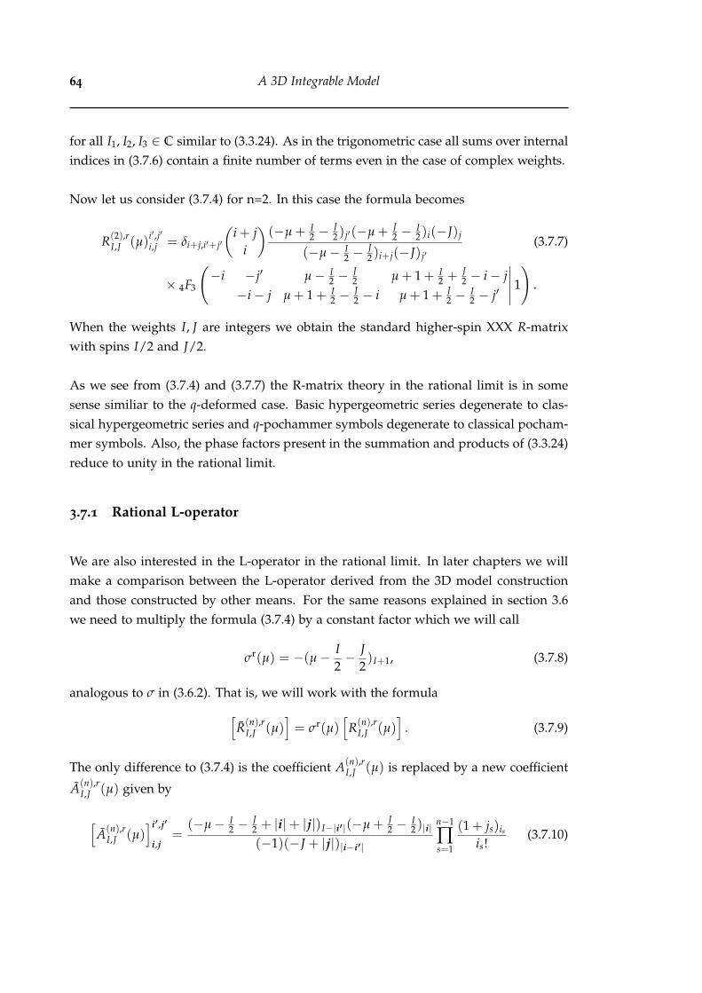
64 A 3D Integrable Model
for all I1, I2, I3 ∈ C similar to (3.3.24). As in the trigonometric case all sums over internalindices in (3.7.6) contain a finite number of terms even in the case of complex weights.
Now let us consider (3.7.4) for n=2. In this case the formula becomes
R(2),rI,J (µ)
i′,j′
i,j = δi+j,i′+j′
(i + j
i
)(−µ + I
2 −J2 )j′(−µ + J
2 −I2 )i(−J)j
(−µ− I2 −
J2 )i+j(−J)j′
(3.7.7)
× 4F3
(−i −j′ µ− I
2 −J2 µ + 1 + I
2 +J2 − i− j
−i− j µ + 1 + I2 −
J2 − i µ + 1 + J
2 −I2 − j′
∣∣∣∣∣ 1
).
When the weights I, J are integers we obtain the standard higher-spin XXX R-matrixwith spins I/2 and J/2.
As we see from (3.7.4) and (3.7.7) the R-matrix theory in the rational limit is in somesense similiar to the q-deformed case. Basic hypergeometric series degenerate to clas-sical hypergeometric series and q-pochammer symbols degenerate to classical pocham-mer symbols. Also, the phase factors present in the summation and products of (3.3.24)reduce to unity in the rational limit.
3.7.1 Rational L-operator
We are also interested in the L-operator in the rational limit. In later chapters we willmake a comparison between the L-operator derived from the 3D model constructionand those constructed by other means. For the same reasons explained in section 3.6we need to multiply the formula (3.7.4) by a constant factor which we will call
σr(µ) = −(µ− I2− J
2)I+1, (3.7.8)
analogous to σ in (3.6.2). That is, we will work with the formula[R(n),r
I,J (µ)]= σr(µ)
[R(n),r
I,J (µ)]
. (3.7.9)
The only difference to (3.7.4) is the coefficient A(n),rI,J (µ) is replaced by a new coefficient
A(n),rI,J (µ) given by
[A(n),r
I,J (µ)]i′,j′
i,j=
(−µ− I2 −
J2 + |i|+ |j|)I−|i′|(−µ + J
2 −I2 )|i|
(−1)(−J + |j|)|i−i′|
n−1
∏s=1
(1 + js)is
is!(3.7.10)
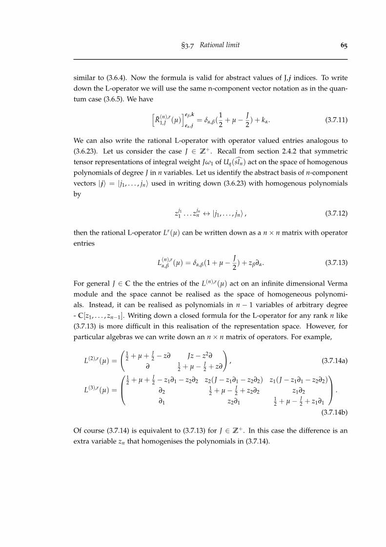
§3.7 Rational limit 65
similar to (3.6.4). Now the formula is valid for abstract values of J,j indices. To writedown the L-operator we will use the same n-component vector notation as in the quan-tum case (3.6.5). We have[
R(n),r1,J (µ)
]eβ,k
eα,j= δα,β(
12+ µ− J
2) + kα. (3.7.11)
We can also write the rational L-operator with operator valued entries analogous to(3.6.23). Let us consider the case J ∈ Z+. Recall from section 2.4.2 that symmetrictensor representations of integral weight Jω1 of Uq(sln) act on the space of homogenouspolynomials of degree J in n variables. Let us identify the abstract basis of n-componentvectors |j〉 = |j1, . . . , jn〉 used in writing down (3.6.23) with homogenous polynomialsby
zj11 . . . zjn
n ↔ |j1, . . . , jn〉 , (3.7.12)
then the rational L-operator Lr(µ) can be written down as a n× n matrix with operatorentries
L(n),rα,β (µ) = δα,β(1 + µ− J
2) + zβ∂α. (3.7.13)
For general J ∈ C the the entries of the L(n),r(µ) act on an infinite dimensional Vermamodule and the space cannot be realised as the space of homogeneous polynomi-als. Instead, it can be realised as polynomials in n − 1 variables of arbitrary degree- C[z1, . . . , zn−1]. Writing down a closed formula for the L-operator for any rank n like(3.7.13) is more difficult in this realisation of the representation space. However, forparticular algebras we can write down an n× n matrix of operators. For example,
L(2),r(µ) =
(12 + µ + J
2 − z∂ Jz− z2∂
∂ 12 + µ− J
2 + z∂
), (3.7.14a)
L(3),r(µ) =
12 + µ + J
2 − z1∂1 − z2∂2 z2(J − z1∂1 − z2∂2) z1(J − z1∂1 − z2∂2)
∂212 + µ− J
2 + z2∂2 z1∂2
∂1 z2∂112 + µ− J
2 + z1∂1
.
(3.7.14b)
Of course (3.7.14) is equivalent to (3.7.13) for J ∈ Z+. In this case the difference is anextra variable zn that homogenises the polynomials in (3.7.14).

66 A 3D Integrable Model
3.7.2 Factorization
Given the reductions (3.5.1), (3.5.2) and factorization (3.5.6) of the trigonometric R-matrix there obviously must exist similar results for the rational R-matrix (3.7.4). Onecan start from (3.7.4) and make the substitutions µ = I − J, I − J ∈ Z+ and µ =
J − I, J − I ∈ Z+ and make the same arguments given in the beginning of section(3.5) but for classical pochammer symbols to find
[R(n),r
I,J (I − J
2)
]i′,j′
i,j= δi+j,i′+j′
(−J)|j|(J − I)|i′−j|(−I)|i′|
n−1
∏s=1
(i′sjs
), I − J ∈ Z+ (3.7.15)
[R(n),r
I,J (J − I
2)
]i′,j′
i,j= δi+j,i′+j′
(−I)|i|(I − J)|j′−i|(−J)|j′|
n−1
∏s=1
(j′sis
), J − I ∈ Z+. (3.7.16)
Of course one could also just take the rational limit of (3.5.1) and (3.5.2). In any case,we can define
Mr(I, J) := R(n),rI,J (
I − J2
), Nr(I, J) := R(n),rI,J (
J − I2
) (3.7.17)
analogous to (3.5.5). Let us note that no similarity transform on (3.7.4) is required hereunlike (3.5.3) and (3.5.4) in the trigonometric case. Functions Mr(I, J), Nr(I, J) dependonly on complex parameters I, J and the dependence is algebraic. Using these functionsthe rational R-matrix R(n),r
I,J (µ) can be written in the factorised form
Proposition 3.7.2.
R(n),rI,J (µ) = Mr(µ +
I + J2
, J)Nr(−µ +I + J
2, J). (3.7.18)
Removing the permutation operator in R gives back the original rational R-matrix(3.7.4), which at the level of matrix elements can be written as
[R(n),r
I,J (λ)]i′,j′
i,j= ∑
k+l=i+jMr k,l
i,j Nr i′,j′
k,l (3.7.19)
where
Mr i′,j′
i,j = δi+j,i′+j′(−J)|j|(−µ + J−I
2 )|i′−j|
(−µ− I+J2 )|i′|
n−1
∏s=1
(i′sjs
), (3.7.20a)
Nr i′,j′
i,j = δi+j,i′+j′(µ− I+J
2 )|j|(−µ + I−J2 )|j′−j|
(−J)|j′|
n−1
∏s=1
(j′sjs
). (3.7.20b)

§3.8 A polynomial representation 67
We will return to these results in later chapters when making comparisons with someother factorisation techniques. To finish this section, we will write down the symmetriesof (3.7.4) which are easily deduced from (3.4.1) - (3.4.6). They are
[R(n),r
I,J (µ)]i′,j′
i,j=[
R(n),rJ,I (µ)
]j′,i′
j,i, (3.7.21a)
=[
R(n),rJ,I (µ)
]τj′,τi′
τj,τi, (3.7.21b)
=n
∏s=1
i′s!j′s!is!js!
[R(n),r
I,J (µ)]τi,τj
τi′,τj′, (3.7.21c)
=[
R(n),rI,J (µ)
]i′,j′
i,j. (3.7.21d)
3.8 A polynomial representation
In the last section we noted that the formula (3.3.24) contains λ in the denominatorterms of the hypergeometric sum and hence each summand is a rational function inthis variable. It would be interesting to determine whether a formula exists where thesummands only contain λ in the numerator and hence are polynomials. We pose thisas a problem; can (3.3.24) be transformed so that the sum only contains λ in the numer-ator?
We can at least give a partial answer to this problem. For n = 2 it can be done us-ing Sears transform for 4φ3 hypergeometric series. For n > 2 we can also do it butonly at the cost of adding extra summations to the expression. As mentioned earlier, atthis stage we are not sure if it is possible to transform without adding extra sums, butif it is then it probably requires some yet to be discovered identities for multivariablehypergeometric series.
In any case, let us take (3.3.30) and apply a similarity transform in the auxiliary spaceby defining
[R(2)
I,J (λ)]i′,j′
i,j= λi−i′
[R(2)
I,J (λ)]i′,j′
i,j. (3.8.1)
It is easy to check that the Yang-Baxter equation is not affected by this modification.Now we make a Sears’ transform (B.2.14) by identifying
n = i, a = q−2j′ , b = λ2q−I−J , c = λ2q2+I+J−2i−2j,

68 A 3D Integrable Model
d = λ2q2+I−J−2i, e = q−2i−2j, f = λ2q2+J−I−2j′ . (3.8.2)
The result is[R(2)
I,J (λ)]i′,j′
i,j= δi+j,i′+j′ (−1)i qi(i+j−2J−1)−I j+i′(I+j′)
λi+i′(q2; q2)i
(q−2J ; q2)j(λ−2q+I−J ; q2)j−i′
(q−2J ; q2)j′(λ−2q−I−J ; q2)i+j
× φ4 3
(q−2i; q−2i′ λ−2qJ−I λ2q2+J−I
q−2I q2(1+j−i′) q2(1+J−i−j)
∣∣∣∣∣ q2, q2
). (3.8.3)
This formula for the Uq(sl2) R-matrix first appeared (up to normalisation) in (5.8) of[10]. Let us note that in writing down this formula we have used the regularisationscheme (B.1.10) and a regularised version of Sears’ transform (B.2.14). The reason weregularise in this way is because the q-pochammer terms in the denominator are ofthe form (q−2n; q2)r which is zero when r > n. Over the summation range from 0 toMin(i, i′) this inequality is sometimes satisfied and the summation is not well defined.However, in all such cases these poles are cancelled off by zeroes in the products outsidethe 4φ3 summation and so the poles are can be removed by our choice of regularisation.
In most cases a regularisation is not necessary. Of course, (3.3.30) does not need it,but there are polynomial representations that mostly do not require it. For example,transforming (3.8.3) using Sears’ transform (B.2.13) with
n = i, a = q−2i′ , c = λ−2q2+J−I , d = λ−2qJ−I ,
d = q−2I , e = q2J−2j−2i+2, f = q2+2j−2i′ ,
and removing regularisation we get the formula
[R(2)
I,J (λ)]i′,j′
i,j= δi+j,i′+j′ qi′ j′−ij+I(i−j′)
[i + j
i
]q2
(q−2I ; q2)i(q−2J ; q2)j(λ−2qI−J ; q2)j−i′
λi+i′(q−2J ; q2)j−i′(λ−2q−I−J ; q2)i+j
× 4φ3
(q−2i q−2i′ λ2q−I−J λ−2q−2−I−J
q−2I q−2(i+j) q−2(J−j+i′)
∣∣∣∣∣ q2, q2
). (3.8.4)
Unlike (3.3.30) and (3.8.3) this series does not appear to always terminate naturally afterfinitely many terms. This is because of the denominator arguments of the form q−m,m ∈ Z+ which can cancel numerator terms that would otherwise terminate the series.However, this series should still be considered to be finite and truncated after i termsbecause it was transformed using identity (B.2.13) which is for finite sums. Of course,there is also the danger of poles from the denominator terms but this is not a problemfor finite-dimensional R-matrices or when I, J are non-integral. In the former case the

§3.8 A polynomial representation 69
sum is truncated before these terms becomes zero and in the latter case the sum termi-nates. The only case where it is a problem is for infinite-dimensional R-matrices whereI, J ∈ Z+ and i(
′) > I, j(′) > J. In this case the expression requires a regularisation such
as (B.1.10).
In the following chapters we want to compare some of the results obtained with (3.8.3)as well as its rational limit q→ 1. Following (3.7.1) - (3.7.3) we get
[R(2),r
I,J (µ)]i′,j′
i,j= δi+j,i′+j′(−1)i (−J)j(−µ + I
2 −J2 )j−i′
i!(−J)j′(−µ− I2 −
J2 )i+j
(3.8.5)
× F4 3
(−i; −i′ −µ + J
2 −I2 µ + 1 + J
2 −I2
−I 1 + j− i′ 1 + J − i− j
∣∣∣∣∣ 1
).
Obviously R(2) and R(2) have the same limit as q → 1 because the leading term in thediagonal similarity transform (3.8.1) is 1.
The n > 2 case is more complicated, and best possible result we have found so farpertains to the rational limit, where we have succeeded at the cost of adding an extrasummation to the expression so that it is an n-fold summation rather than an (n− 1)-fold summation like (3.3.24) and (3.7.4). It would be nice to find a (n− 1)-fold summa-tion polynomial formula but it is at this stage unclear to us if it exists. In any case, wehave found that
[R(n),r
I,J (µ)]i′,j′
i,j= δi+j,i′+j′
(−I)|i|(−J)|j|(−µ + I−J2 )|j−i′|
(−J)|j−i′|(−µ− I+J2 )|i+j|
n−1
∏s=1
(is + js
is
)
× ∑m,mn
(µ + I+J2 − |i + j|+ 1)|m|
(−|i|,−|i′|)|m|(−|i|,−|i′|, µ− I+J
2 )|m|+mn
mn!(−I, J − |j|+ |i′|)|m|+mn
n−1
∏s=1
(−1)ms(−is,−i′s)ms
ms!(−is − js)ms
,
where m = m1, . . . mn−1 as in (3.7.4), 0 ≤ m ≤ i and 0 ≤ mn ≤ |i−m|. We note thatfor finite matrices and non-integral Verma modules I, J ∈ C the formula does not needregularisation.

70 A 3D Integrable Model

Chapter 4
Spectral decomposition
In this chapter we will review another method for constructing R-matrices. This methodwe will refer to as spectral decomposition. This method is well known in the literature[16; 17; 18], and is perhaps the oldest of all the approaches considered in this thesis. Itis quite different to the 3D model approach of the last chapter because it uses quantumgroups and their representation theory directly. We are interested in constructing theR-matrix using this approach and comparing it with the other newer constructions.
We can show that at least for Uq(sl2) the R-matrix is the same as that obtained from the3D approach. To show this we construct an explicit formula for the matrix elements forfinite-dimensional highest weight representations. The formula at first sight appears tobe very different to (3.3.24) obtained in Chapter 3 with very different structure. It turnsout both formulas actually produce the same output and to prove they are indeed thesame we will give the transformation between the two.
First we will give an overview of the method including all of the relevant theory andthen we will apply it to the case of Uq(sl2).
4.1 The Jimbo equations
Perhaps the central idea behind this method is notion of the R-Matrix as an intertwinerof two quantum group representations. Let us recall (2.4.43)
R∆(g) = ∆op(g)R ∀g ∈ A, (4.1.1)
71

72 Spectral decomposition
satisfied by the universal R-matrix. Because ∆ is an algebra homomorphism it is enoughto consider the relation on the generators of Uq(g). Indeed, for Uq(sln) under the eval-uation homomorphism (2.4.52) the relation (4.1.1) can be written as n separate relations
R(x, y)∆(Ei) = ∆op(Ei)R(x, y) 1 ≤ i ≤ n, (4.1.2a)
R(x, y)(xGFθ ⊗ qHθ/2 + q−Hθ/2 ⊗ yGFθ)
= (yGFθ ⊗ q−Hθ/2 + qHθ/2 ⊗ xGFθ)R(x, y) (4.1.2b)
for the universal R-matrix and coproduct. Taking two affinisable finite-dimensionalrepresentations π I , π J and applying π I ⊗ π J to these relations as in (2.4.60) we get a setof linear equations that can be solved for RI,J(λ), λ = x/y. Just like (2.4.60) we willdenote the representation map π I ⊗ π J applied to ∆ by
∆I,J(a) := (π I ⊗ π J)(∆(a)). (4.1.3)
It is true that π I ⊗ π J is a representation of Uq(g)⊗Uq(g) on the representation spaceVI ⊗VJ . That is,
π I ⊗ π J : Uq(g)⊗Uq(g)→ End(VI)⊗ End(VJ), (4.1.4)
(π I ⊗ π J)(a⊗ b) · (v⊗ u) = (π I(a) · v)⊗ (π J(b) · u) ∀a, b ∈ g⊗ g (4.1.5)
and End(VI)⊗ End(VJ) ∼= End(VI ⊗ VJ) at least for the finite dimensional representa-tion spaces we consider.
Due to Hopf algebra structure of the quantum group ∆ is an algebra homomorphismand hence ∆I,J can be viewed as a representation of Uq(g) on the space VI ⊗ VJ -the pullback of π I ⊗ π J by ∆. With this in mind let us define a modified R-MatrixRI,J : VI ⊗VJ → VJ ⊗VI by
RI,J = PRI,J , P(v⊗ u) = u⊗ v, (4.1.6)
and rewrite the relations (4.1.2) in terms of RI,J(λ) for a given representation ∆I,J . Wehave
RI,J(λ)∆I,J(a) = ∆J,I(a)RI,J(λ), ∀a ∈ Uq(g), (4.1.7a)
RI,J(λ)(λπ I(GFθ)⊗ π J(qHθ/2) + π I(q−Hθ/2)⊗ π J(GFθ))
= (π J(GFθ)⊗ π I(qHθ/2) + λπ J(q−Hθ/2)⊗ π I(GFθ))RI,J(λ). (4.1.7b)
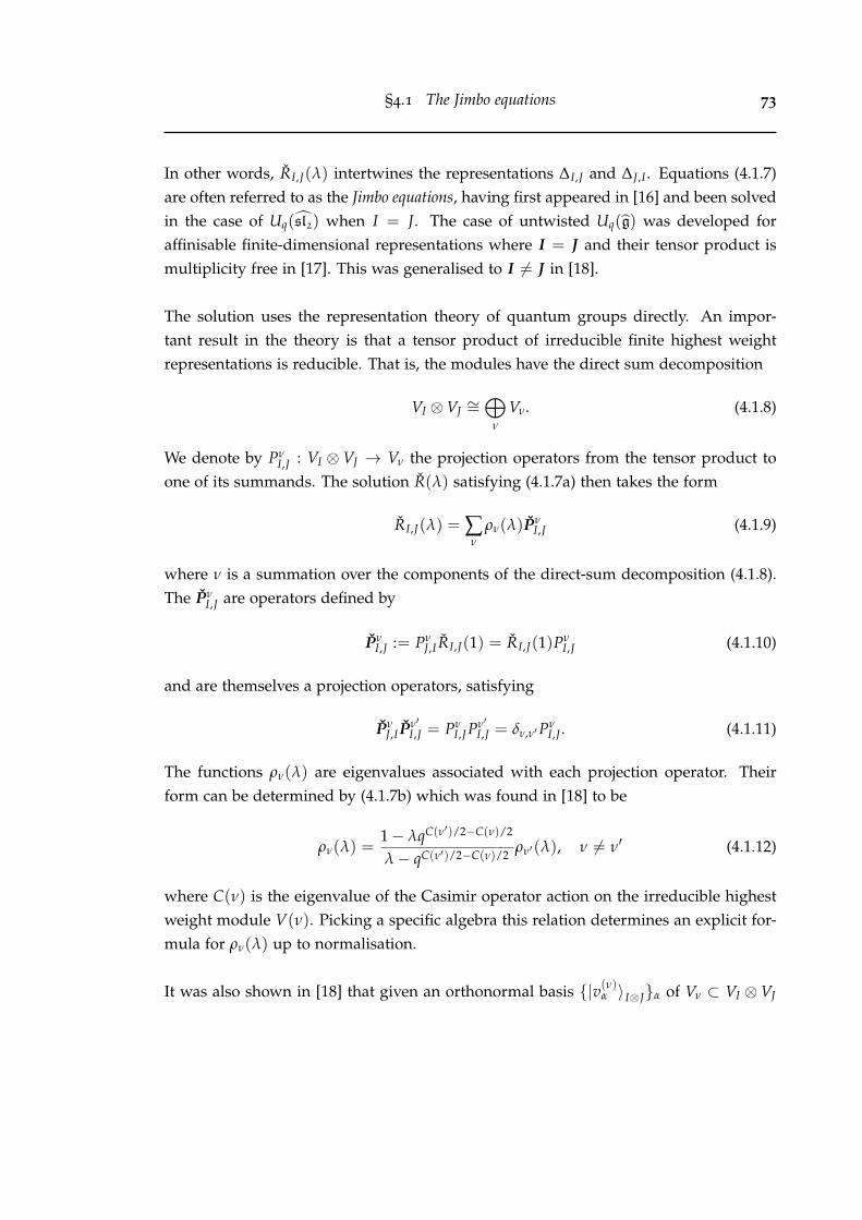
§4.1 The Jimbo equations 73
In other words, RI,J(λ) intertwines the representations ∆I,J and ∆J,I . Equations (4.1.7)are often referred to as the Jimbo equations, having first appeared in [16] and been solvedin the case of Uq(sl2) when I = J. The case of untwisted Uq(g) was developed foraffinisable finite-dimensional representations where I = J and their tensor product ismultiplicity free in [17]. This was generalised to I 6= J in [18].
The solution uses the representation theory of quantum groups directly. An impor-tant result in the theory is that a tensor product of irreducible finite highest weightrepresentations is reducible. That is, the modules have the direct sum decomposition
VI ⊗VJ ∼=⊕
ν
Vν. (4.1.8)
We denote by PνI,J : VI ⊗ VJ → Vν the projection operators from the tensor product to
one of its summands. The solution R(λ) satisfying (4.1.7a) then takes the form
RI,J(λ) = ∑ν
ρν(λ)PνI,J (4.1.9)
where ν is a summation over the components of the direct-sum decomposition (4.1.8).The Pν
I,J are operators defined by
PνI,J := Pν
J,I RI,J(1) = RI,J(1)PνI,J (4.1.10)
and are themselves a projection operators, satisfying
PνJ,IP
ν′I,J = Pν
I,J Pν′I,J = δν,ν′Pν
I,J . (4.1.11)
The functions ρν(λ) are eigenvalues associated with each projection operator. Theirform can be determined by (4.1.7b) which was found in [18] to be
ρν(λ) =1− λqC(ν′)/2−C(ν)/2
λ− qC(ν′)/2−C(ν)/2ρν′(λ), ν 6= ν′ (4.1.12)
where C(ν) is the eigenvalue of the Casimir operator action on the irreducible highestweight module V(ν). Picking a specific algebra this relation determines an explicit for-mula for ρν(λ) up to normalisation.
It was also shown in [18] that given an orthonormal basis |v(ν)α 〉I⊗Jα of Vν ⊂ VI ⊗ VJ
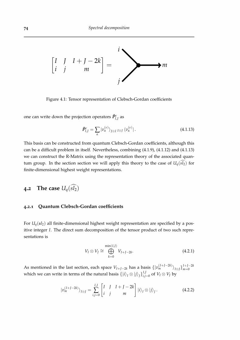
74 Spectral decomposition
[I J I + J − 2ki j m
]=
i
j
m
Figure 4.1: Tensor representation of Clebsch-Gordan coefficients
one can write down the projection operators PνI,J as
PνI,J = ∑
α
|v(ν)α 〉J⊗I I⊗J 〈v(ν)α | . (4.1.13)
This basis can be constructed from quantum Clebsch-Gordan coefficients, although thiscan be a difficult problem in itself. Nevertheless, combining (4.1.9), (4.1.12) and (4.1.13)we can construct the R-Matrix using the representation theory of the associated quan-tum group. In the section section we will apply this theory to the case of Uq(sl2) forfinite-dimensional highest weight representations.
4.2 The case Uq(sl2)
4.2.1 Quantum Clebsch-Gordan coefficients
For Uq(sl2) all finite-dimensional highest weight representation are specified by a pos-itive integer I. The direct sum decomposition of the tensor product of two such repre-sentations is
VI ⊗VJ ∼=min(I,J)⊕
k=0
VI+J−2k. (4.2.1)
As mentioned in the last section, each space VI+J−2k has a basis |v(I+J−2k)m 〉I⊗J
I+J−2km=0
which we can write in terms of the natural basis |i〉I ⊗ |j〉JI,Ji,j=0 of VI ⊗VJ by
|v(I+J−2k)m 〉I⊗J =
I,J
∑i,j=0
[I J I + J − 2ki j m
]|i〉I ⊗ |j〉J . (4.2.2)
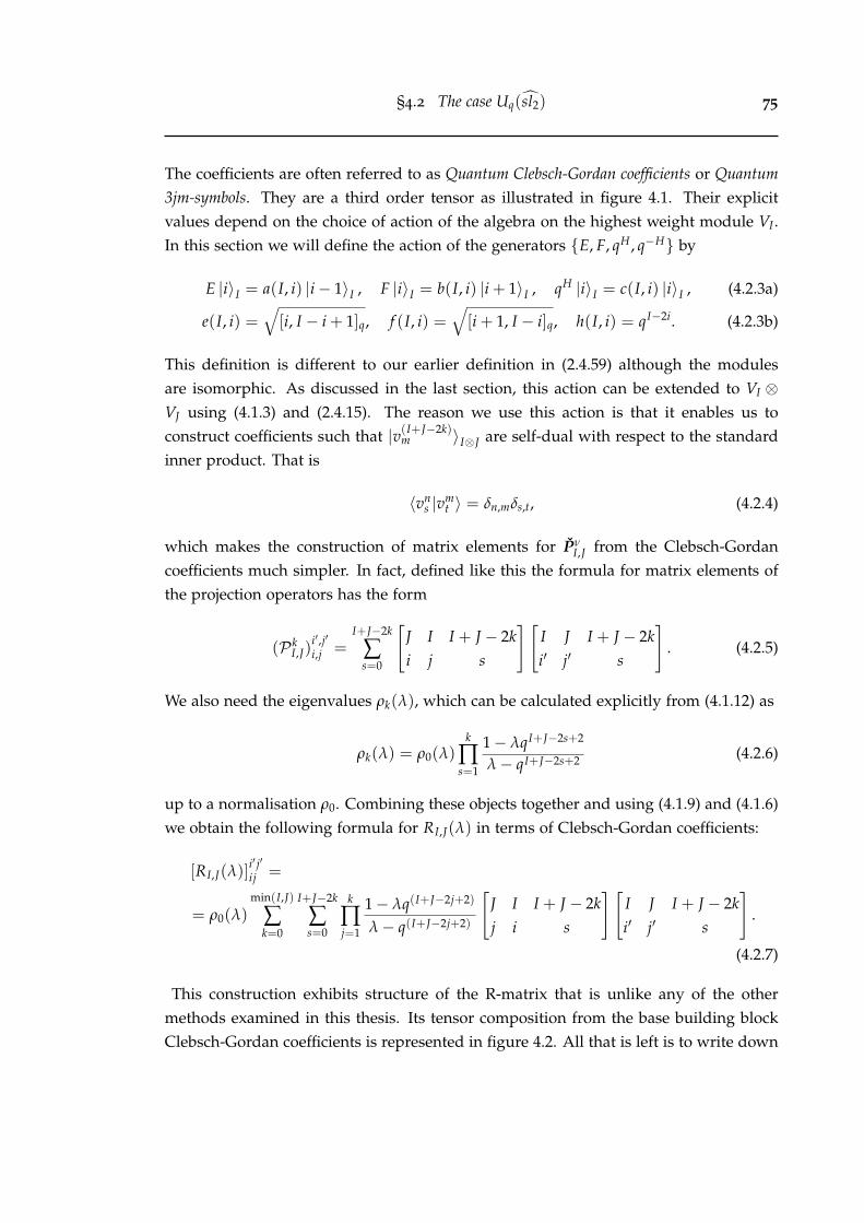
§4.2 The case Uq(sl2) 75
The coefficients are often referred to as Quantum Clebsch-Gordan coefficients or Quantum3jm-symbols. They are a third order tensor as illustrated in figure 4.1. Their explicitvalues depend on the choice of action of the algebra on the highest weight module VI .In this section we will define the action of the generators E, F, qH, q−H by
E |i〉I = a(I, i) |i− 1〉I , F |i〉I = b(I, i) |i + 1〉I , qH |i〉I = c(I, i) |i〉I , (4.2.3a)
e(I, i) =√[i, I − i + 1]q, f (I, i) =
√[i + 1, I − i]q, h(I, i) = qI−2i. (4.2.3b)
This definition is different to our earlier definition in (2.4.59) although the modulesare isomorphic. As discussed in the last section, this action can be extended to VI ⊗VJ using (4.1.3) and (2.4.15). The reason we use this action is that it enables us toconstruct coefficients such that |v(I+J−2k)
m 〉I⊗J are self-dual with respect to the standardinner product. That is
〈vns |vm
t 〉 = δn,mδs,t, (4.2.4)
which makes the construction of matrix elements for PνI,J from the Clebsch-Gordan
coefficients much simpler. In fact, defined like this the formula for matrix elements ofthe projection operators has the form
(P kI,J)
i′,j′
i,j =I+J−2k
∑s=0
[J I I + J − 2ki j s
] [I J I + J − 2ki′ j′ s
]. (4.2.5)
We also need the eigenvalues ρk(λ), which can be calculated explicitly from (4.1.12) as
ρk(λ) = ρ0(λ)k
∏s=1
1− λqI+J−2s+2
λ− qI+J−2s+2 (4.2.6)
up to a normalisation ρ0. Combining these objects together and using (4.1.9) and (4.1.6)we obtain the following formula for RI,J(λ) in terms of Clebsch-Gordan coefficients:
[RI,J(λ)]i′ j′
ij =
= ρ0(λ)min(I,J)
∑k=0
I+J−2k
∑s=0
k
∏j=1
1− λq(I+J−2j+2)
λ− q(I+J−2j+2)
[J I I + J − 2kj i s
] [I J I + J − 2ki′ j′ s
].
(4.2.7)
This construction exhibits structure of the R-matrix that is unlike any of the othermethods examined in this thesis. Its tensor composition from the base building blockClebsch-Gordan coefficients is represented in figure 4.2. All that is left is to write down

76 Spectral decomposition
[R(λ)]i′,j′
i,j = ∑k
ρk(λ)
j
i
i′
j′
s
Figure 4.2: R-matrix representation as a sum of projection operators
the expression for these coefficients and we have a formula for the matrix elements ofRI,J(λ). The coefficients we use are given by[
I J I + J − 2ki j m
]= δi+j,k+m(−1)i+jq−j2+mj−2ij−2kj+(i−k)(J−k)
×
√(q2; q2)i(q2; q2)J−j(q2; q2)I−k(q2; q2)I+J−2k−m(q4; q2)I+J−2k
(q2; q2)j(q2; q2)I−i(q2; q2)J−k(q2; q2)k(q2; q2)m(q4; q2)I+J−k
× 3φ2
(q−2j; q−2m q2+2J−2j
q2+2i−2m q2i−2m−2I
∣∣∣∣∣ q2, q2i+2j+2k−2I−2J
). (4.2.8)
We constructed this formula using the action (4.2.3). The highest weight vector |vν0〉I⊗J
in each submodule can be identified by solving
∆I,J(E) · |vν0〉I⊗J = 0.
The string basis of each submodule can be generated by repeated applications of the‘lowering operator’ F to the highest weight vector. That is,
|vνm〉I⊗J = ∆I,J(Fm) · |vν
0〉I⊗J .
Some analysis of (4.2.8) is warranted. One can use the Karlsson-Minton summationformula (B.2.4) on the 3φ2 hypergeometric series with
a = q−2j, b1 = q2i−2m−2I , m1 = I − i,
b2 = q2+2i−2m, m2 = J + m− i− j,
to see that the quantum Clebsch-Gordon coefficients are non-trivially zero wheneverm > I + J − 2k. In addition, it is easy to see that the expression is trivially zero whenm < 0 due to the (q2; q2)m q-Pochhammer in the denominator.

§4.2 The case Uq(sl2) 77
This analysis is important when reducing the quadruple sum in (4.2.7) to a triple sum.The conservation law δi+j,m+k in (4.2.8) allows us to eliminate the sum over ‘s’ in (4.2.7).In doing so the sum over ‘k’ may include terms containing Clebsch-Gordon coefficientswith arguments outside its domain. In particular, it may happen that the inequality0 ≤ m ≤ I + J − 2k is broken. Due to the discussion in the previous paragraph theseterms will always be zero and not contribute to the sum.
4.2.2 An explicit formula
The conservation laws of both Clebsch-Gordon coefficients in (4.2.7) imply the conserva-tion law δi+j,i′+j′ for the R-matrix. After substituting (4.2.8) into (4.2.7), setting ρ0(λ) = 1and simplifying with q-Pochhammer identities we find the triple sum expression
[RI J(λ)]i′,j′
i,j = δi+j,i′+j′Ti′,j′
i,j
qi(3I+5J−2j+4)+j(3I+2J+2) (q2; q2)i′(q2; q2)
I+J−i−j
(q2; q2)
J−j′
qi′(I+2J+2) (q2; q2)i (q2; q2)i+j (q2; q2)I+J (q2; q2)J−j
×∑r
(−1)rλr (λ−1q−I−J , q−2i−2j, q−2I−2J−2; q2)r
(q−2I−2J ; q2)
2r
qr(I+J+1+2j′−2j)−r2 (q2, λq−I−J , q2i−2I+2j−2J ; q2)
r (q−2I−2J−2; q2)2r
× 3φ2
(q−2i; q−2i+2I+2 q−2i−2j+2r
q−2i+2r+2 q−2i−2J+2r
∣∣∣∣∣ q2, q2i−2I+2j−2J+2r
)
× 3φ2
(q−j′ ; q−2i′−2j′+2r q2J−2j′+2
q2r−2j′+2 q−2I−2j′+2r
∣∣∣∣∣ q2, q2i′−2I+2j′−2J+2r
)(4.2.9)
for elements of the R-matrix where
Ti′,j′
i,j =
√√√√ (q2, q2)i (q2, q2)j (q−2I , q2)i′ (q−2J , q2)j′
(q2, q2)i′ (q2, q2)j′ (q−2I , q2)i (q−2J , q2)j. (4.2.10)
The sum over ‘r’ is finite and over the range 0 ≤ r ≤ min(I, J, i + j, I + J − i− j). Thisis a refinement of the upper bound in (4.2.7) where it is min(I, J) because the sum canterminate sooner than this in a couple of ways. First, the q-Pochhammer
(q−2i−2j; q2)
rin the numerator will have a zero whenever r > i + j which may be a smaller boundand therefore terminating the sum earlier. Second, it may happen that r > I + J − i− jand therefore the q-Pochhamer
(q2i−2I+2j−2J ; q2)
r in the denominator is zero. However,this pole is cancelled by the double zero (implied by (B.2.4)) of the two Clebsch-Gordon
3φ2 hypergeometric series and therefore no terms when r > I + J − i− j contribute tothe sum. Therefore summing over ‘r’ from 0 to min(I, J, i + j, I + J − i− j) includes all
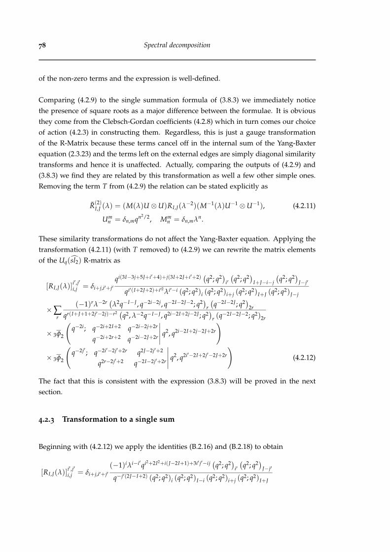
78 Spectral decomposition
of the non-zero terms and the expression is well-defined.
Comparing (4.2.9) to the single summation formula of (3.8.3) we immediately noticethe presence of square roots as a major difference between the formulae. It is obviousthey come from the Clebsch-Gordan coefficients (4.2.8) which in turn comes our choiceof action (4.2.3) in constructing them. Regardless, this is just a gauge transformationof the R-Matrix because these terms cancel off in the internal sum of the Yang-Baxterequation (2.3.23) and the terms left on the external edges are simply diagonal similaritytransforms and hence it is unaffected. Actually, comparing the outputs of (4.2.9) and(3.8.3) we find they are related by this transformation as well a few other simple ones.Removing the term T from (4.2.9) the relation can be stated explicitly as
R(2)I,J (λ) = (M(λ)U ⊗U)RI,J(λ
−2)(M−1(λ)U−1 ⊗U−1), (4.2.11)
Umn = δn,mqn2/2, Mm
n = δn,mλn.
These similarity transformations do not affect the Yang-Baxter equation. Applying thetransformation (4.2.11) (with T removed) to (4.2.9) we can rewrite the matrix elementsof the Uq(sl2) R-matrix as
[RI,J(λ)]i′,j′
i,j = δi+j,i′+j′qi(3I−3j+5J+i′+4)+j(3I+2J+i′+2) (q2; q2)
i′(q2; q2)
I+J−i−j
(q2; q2)
J−j′
qi′(I+2J+2)+i′2 λi′−i (q2; q2)i (q2; q2)i+j (q2; q2)I+J (q2; q2)J−j
×∑r
(−1)rλ−2r (λ2q−I−J , q−2i−2j, q−2I−2J−2; q2)r
(q−2I−2J ; q2)
2r
qr(I+J+1+2j′−2j)−r2 (q2, λ−2q−I−J , q2i−2I+2j−2J ; q2)
r (q−2I−2J−2; q2)2r
× 3φ2
(q−2i; q−2i+2I+2 q−2i−2j+2r
q−2i+2r+2 q−2i−2J+2r
∣∣∣∣∣ q2, q2i−2I+2j−2J+2r
)
× 3φ2
(q−2j′ ; q−2i′−2j′+2r q2J−2j′+2
q2r−2j′+2 q−2I−2j′+2r
∣∣∣∣∣ q2, q2i′−2I+2j′−2J+2r
)(4.2.12)
The fact that this is consistent with the expression (3.8.3) will be proved in the nextsection.
4.2.3 Transformation to a single sum
Beginning with (4.2.12) we apply the identities (B.2.16) and (B.2.18) to obtain
[RI,J(λ)]i′,j′
i,j = δi+j,i′+j′(−1)iλi−i′qi2+2I2+i(J−2I+1)+3i′ j′−ij (q2; q2)
i′(q2; q2)
J−j′
q−j′(2J−I+2) (q2; q2)i (q2; q2)I−i (q2; q2)i+j (q2; q2)I+J

§4.2 The case Uq(sl2) 79
×∑r
q2r(i+j)+r(I+J)−2r2λ−2r (λ2q−I−J , q−2i−2j, q−2I−2J−2; q2)
r
(q−2I−2J ; q2)
2r(λ−2q−I−J , q2)r (q−2I−2J−2; q2)2r
× 3φ2
(q2r−2I ; q2i−2I q2J−2r+2
q−2I q2i−2I+2j+2
∣∣∣∣∣ q2, q2
)3φ2
(q−2j′ ; q2r−2J q2I−2r+2
q−2J q−2i+2I−2j+2
∣∣∣∣∣ q2, q−2i′)
.
(4.2.13)
The summation range for r is the same as it was in equation (4.2.9). We rewrite (4.2.13)by bringing out the summations in the 3φ2 series outside the sum over ‘r’ - denotingtheir summation indices by ‘s’ and ‘l’ respectively. In doing so we notice that the sumover ‘r’ is a very-well-poised 6φ5 series. More explicitly,
[RI,J(λ)]i′,j′
i,j = λi−i′(−1)I+j+i′ q2i2+i(−3I+j+J+i′+2)(q2; q2)I(q2; q2)J
qI(1−I)+(i′−j)(j+2i′+1−I)(q2; q2)I+J
× (q2; q2)I−i′(q2; q2)i′
(q2; q2)I−i(q2; q2)i
j′,I−i
∑l,s=0
q2s−2li′(q−2j′ , q2I+2, q2)l(q2J+2, q2i−2I ; q2)
s(q2; q2)l (q2; q2)s (q2; q2)I+l−i−j (q2; q2)i+j+s−I
× 6φ5
(q−2I−2J−2 −q−I−J+1 q−I−J+1 λ2q−I−J q2l−2J q2s−2I
−q−I−J−1 q−I−J−1 q−I−J
λ2 q−2I−2l q−2J−2s
∣∣∣∣∣ q2,qI+J−2l−2s
λ2
).
(4.2.14)
Interestingly, this series depends only on λ, I and J, a fact elaborated on in section4.2.4. Even though the 6φ5 series has denominator terms of the form q−m, m ∈ Z+ thissum does not have any poles because of the range of the summation over ‘r’ explainedafter equation (4.2.9). Therefore this series is truncated before the denominator termscan be zero. In fact, by noting the range of the sums over ‘s’ and ‘l’ the range of thesummation over ‘r’ can be re-expressed as 0 ≤ r ≤ min(I − s, J − l). We use identity(B.2.5) with a = q−2I−2J−2 and n = I − s to write the 6φ5 series as a product. The triplesum therefore reduces to a double sum. Identifying the sum over ‘l’ as a 3φ2 series wehave
[RI,J(λ)]i′,j′
i,j = δi+j,i′+j′(−1)j′λ3i−i′−2Iqi2+I(I−J−2)+i(j+i′+3−2I)+(j−i′)(j+2i′+1−I)
× (q2; q2)i′(q2; q2)I−i′(λ−2qJ−I ; q2)i
(q2; q2)i(q2; q2)j(q2; q2)I−i(λ−2q−I−J ; q2)I
j′
∑l=0
q−2li′(q−2j′ , λ2qI−J+2; q2)l
(q2; q2)I+l−i−j(λ2q−2i+I−J+2; q2)l
× 3φ2
(q−2I+2i; λ2q−I+J+2 q2l+2
λ2q−I−J+2l+2 q2i−2I+2j+2
∣∣∣∣∣ q2, q2
). (4.2.15)
Transforming the 3φ2 using identity (B.2.19) we see that (4.2.15) becomes
[RI,J(λ)]i′,j′
i,j = δi+j,i′+j′(−1)i+i′λi−2j−i′qi2+2j2−2i′2−jJ+i(j−J+i′−I+1)+i′(I+j−1)

80 Spectral decomposition
× (q2, q2)i′(q2, q2)I−i′(λ−2qJ−I , q2)i
(q2, q2)i(q2, q2)j(q2, q2)I−i(λ−2q−I−J , q2)i+j
j′
∑l=0
q−2li′(q−2j′ , λ2qI−J+2, q2)l
(q2, λ2qI−J−2i+2, q2)l
× 3φ2
(q−2j; λ2q−I−J λ2qI+J−2i−2j+2
λ2qI−J−2i−2j+2l+2 λ2qJ−I−2j+2
∣∣∣∣∣ q2, q2l+2
). (4.2.16)
Now rewriting (4.2.16) by interchanging the order of the two sums, the sum over ‘l’ canbe identified as a terminating 2φ1 series. That is,
[RI,J(λ)]i′,j′
i,j = δi+j,i′+j′(−1)i+i′λj+j′ qi2−2i′2−i(I+J+j−i′−1)(q2; q2)i′(q2; q2)I−i′
qi′(1−I)+j(J−i′−2)(q2; q2)i(q2; q2)j(q2; q2)I−i
×(λ−2qI−J ; q2)j(λ
−2qJ−I ; q2)i+j
(λ−2q−I−J ; q2)i+j
j
∑s=0
q2s(q−2j, λ2q−I−J , λ2qI+J−2i−2j+2; q2)s
(q2, λ2qJ−I−2j+2, λ2qI−J−2i−2j+2; q2)s
× 2φ1
(q−2j′ λ2qI−J+2
λ2qI−J−2i−2j+2s+2
∣∣∣∣∣ q2, q2s−2i′)
. (4.2.17)
The 2φ1 series can written as a product of binomials using the q-Chu-Vandermondesum (B.2.2) with n = j′. Doing so yields the single summation
[RI,J(λ)]i′,j′
i,j = δi+j,i′+j′qi′ j′−ij−I j−Ji′[
i + ji
]q2
(λ−2qJ−I ; q2)i′(λ−2qI−J ; q2)j(q−2I ; q2)i
λi−i′(λ−2q−I−J ; q2)i+j(q−2I ; q2)i′
× 4φ3
(q−2j q−2i′ λ2q−I−J λ2qI+J−2i−2j+2
q−2i−2j λ2qJ−I−2j+2 λ2qI−J−2i′+2
∣∣∣∣∣ q2, q2
). (4.2.18)
This is just (3.3.30) under the symmetry (3.4.1) and the similarity transform (3.8.1). Wealready showed this is equal to (3.8.3) using the Sears’ transform (B.2.14) with iden-tification (3.8.2). Therefore we have linked the two constructions and shown that theconstructed R-matrix is the same.
4.2.4 Discussion
In transforming (4.2.13) to (4.2.14) we realised the summation over ‘r’ as a 6φ5 very-well-poised basic hypergeometric series that can be written as a product of binomials.This product depends only on λ, I, and J and not at all on indices i, j, i′, j′. Moreover, theremaining summations do not depend on λ and are split into summations dependingonly on lower or upper indices. In other words, we can write (4.2.15) in the form

§4.2 The case Uq(sl2) 81
[R(λ)]i′,j′
i,j =
i
j
i′
j′
s lA C
B(λ)
Figure 4.3: Graphical representation of the R-matrix (4.2.19)
Proposition 4.2.1.
[RI,J(λ)]i′,j′
i,j = δi+j,i′+j′λi−i′κ ∑
s,lAs
i,jBls(λ)C
i′,j′
l (4.2.19)
where
Asi,j = (−1)j q2i2+j2+ij+j(1−I)+i(2−3I+J)+2s(q2i−2I ; q2)s
(q2; q2)s(q2; q2)i(q2; q2)I−i(q2; q2)s+i+j−I, (4.2.20a)
Bls(λ) =
(q2; q2)s+l(λ2q2+I−J ; q2)l(λ
2q2+J−I ; q2)s
(λ2q2−I−J ; q2)s+l, (4.2.20b)
Ci′,j′
l = (−1)i′ qi′ j′−i′2+i′(I−1)−2li′(q−2j′ ; q2)l(q2; q2)I−i′(q2; q2)i′
(q2; q2)l(q2; q2)l+I−i′−j′, (4.2.20c)
κ = (−1)IqI2−I J−I (λ−2qJ−I ; q2)I
(λ−2q−I−J ; q2)I. (4.2.20d)
The summation indices s, l have the same range as they do in (4.2.13). κ is a multiplica-tion of the R-matrix by a constant and the λi−i′ term is a gauge transform whose pres-ence does not affect the Yang-Baxter equation - both terms can be removed if desired.A graphical representation of this factorisation is presented in figure 4.3. Althoughthe operators A and B have the same valence as the Clebsch-Gordan coefficients, theirelements are very different, given by binomial products rather than 3φ2 basic hyperge-ometric series.

82 Spectral decomposition

Chapter 5
R-matrix factorisation byQ-operators
In this chapter we will review a factorisation of the R-matrix first introduced by Derka-chov in [13] and developed by Derkachov-Manashhov in [66]. It is a factorisation ofrational R-matrices with SL(N, C) symmetry in terms of ‘elementary’ intertwining op-erators which are closely related to Baxter Q-operators [41]. We are particularly inter-ested to compare the factorisation (3.5.6) obtained from the 3D model approach to theone here. Already we can note some important similarities and differences. Firstly, thefactorisation (3.5.6) is for trigonometric R-matrices and so is a deformation of those con-structed by Derkachov. A direct comparison is only possible after taking the rationallimit q → 1 as we did in (3.7.4). In this case, the rational limit of (3.5.6) - which wefound to be (3.7.19) - is written as a product of two almost equal factors for symmet-ric tensor representations of sln while Derkachov’s factorisation for the same algebracontains n factors for any lowest weight representation. For the case n = 2 it turnsout that the factorizations are exactly the same. For n > 2 however the situation ismore complicated and it would be interesting to see how the n factors in Derkachov’sconstruction reduce to the 2 stochastic R-matrices (3.5.8) in the restriction to symmetrictensor representations.
Derkachov’s construction [66] uses the principal series representations of the Lie groupSL(n, C) to construct the R-operator that acts on this representation space and is invari-ant with respect to the Lie group action. The representation space is characterised asthe space of functions in n(n − 1)/2 variables and the R-operator is represented in afactorised form consisting of integral operators. The restriction of these operators to thespace of polynomials [13] is equivalent to the R-matrix acting on Verma modules of sln.
83

84 R-matrix factorisation by Q-operators
The main advantage of this approach is that it constructs the R-matrix for any rep-resentation of sln. In the process we also construct elementary factors that are veryclosely related to local operators used to construct Baxter Q-operators. That means wecan potentially generalise the formulae obtained in chapter 3 using the 3-dimensionalapproach. In this thesis we will consider the explicit construction of the R-matrix for thecase n = 2, 3. For higher rank algebras the problem is no more difficult conceptually,but the computational challenge grows considerably with n, and at the time of writingthis is still in the process of being solved.
In the first part of this chapter we will give an overview of the construction and thenwe will compute formulae for matrix elements of all the operators involved in the con-struction for n = 2, 3. We will then analyse and discuss the results.
5.1 Factorized ansatz
This factorisation approach can be seen as an alternative way of solving the Yang-Baxter RLL-relation, which we introduced in a particular case in (2.4.4). There it waspresented as an equality of operators acting on Cn⊗Cn⊗V3 so that R12 acts on a finitedimensional vector space. In this chapter we will consider the same equation but actingon V1⊗V2⊗C2 (in the case of sl2) so thatR12 is an operator acting on V1⊗V2 ∼= VI ⊗VJ
with arbitrary weight parameters I and J. Both forms are a restriction of the generalYang-Baxter equation (2.3.25) to certain integral weights. Here we will rewrite the RLL-relation but with additive spectral parameters u, v as
R12(u− v)L1(u)L2(v) = L2(v)L1(u)R12(u− v). (5.1.1)
For a fixed L-operator Li acting non-trivially on Vi ⊗ Cm this equation determines theR-matrix R12(u − v) with arbitrary weights I, J. For example, in [13] the L-operatoracting in Vl ⊗C2 is given by
L(u) = u + 2S⊗ s + S− ⊗ s+ + S+ ⊗ s− =
(u + S S−
S+ u− S
), (5.1.2)
where S, S± are generators of the sl2 Lie algebra acting in the lowest weight repre-sentation space Vl with spin parameter l. These generators are related to E1, F1, H1presented in (2.4.21) by 2S = H1, S+ = E1, and S− = F1. The operators s, s± are the
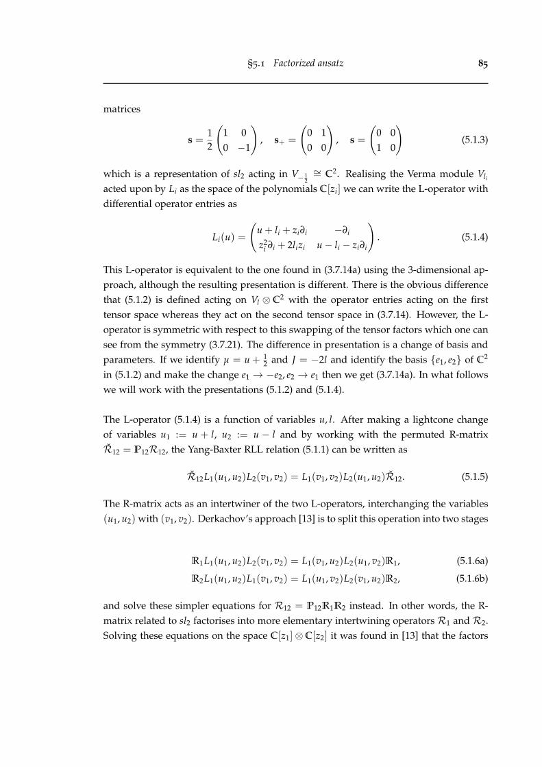
§5.1 Factorized ansatz 85
matrices
s =12
(1 00 −1
), s+ =
(0 10 0
), s =
(0 01 0
)(5.1.3)
which is a representation of sl2 acting in V− 12
∼= C2. Realising the Verma module Vli
acted upon by Li as the space of the polynomials C[zi] we can write the L-operator withdifferential operator entries as
Li(u) =
(u + li + zi∂i −∂i
z2i ∂i + 2lizi u− li − zi∂i
). (5.1.4)
This L-operator is equivalent to the one found in (3.7.14a) using the 3-dimensional ap-proach, although the resulting presentation is different. There is the obvious differencethat (5.1.2) is defined acting on Vl ⊗ C2 with the operator entries acting on the firsttensor space whereas they act on the second tensor space in (3.7.14). However, the L-operator is symmetric with respect to this swapping of the tensor factors which one cansee from the symmetry (3.7.21). The difference in presentation is a change of basis andparameters. If we identify µ = u + 1
2 and J = −2l and identify the basis e1, e2 of C2
in (5.1.2) and make the change e1 → −e2, e2 → e1 then we get (3.7.14a). In what followswe will work with the presentations (5.1.2) and (5.1.4).
The L-operator (5.1.4) is a function of variables u, l. After making a lightcone changeof variables u1 := u + l, u2 := u − l and by working with the permuted R-matrixR12 = P12R12, the Yang-Baxter RLL relation (5.1.1) can be written as
R12L1(u1, u2)L2(v1, v2) = L1(v1, v2)L2(u1, u2)R12. (5.1.5)
The R-matrix acts as an intertwiner of the two L-operators, interchanging the variables(u1, u2) with (v1, v2). Derkachov’s approach [13] is to split this operation into two stages
R1L1(u1, u2)L2(v1, v2) = L1(v1, u2)L2(u1, v2)R1, (5.1.6a)
R2L1(u1, u2)L1(v1, v2) = L1(u1, v2)L2(v1, u2)R2, (5.1.6b)
and solve these simpler equations for R12 = P12R1R2 instead. In other words, the R-matrix related to sl2 factorises into more elementary intertwining operators R1 and R2.Solving these equations on the space C[z1]⊗C[z2] it was found in [13] that the factors

86 R-matrix factorisation by Q-operators
are given (up to normalization) by
R1(u1|v1, v2) =Γ(z21∂2 + u1 − v2)
Γ(z21∂2 + v1 − v2), (5.1.7a)
R2(u1, u2|v2) =Γ(z12∂1 + u1 − v2)
Γ(z12∂1 + u1 − u2)(5.1.7b)
where zij = zi − zj. The sl2 R-matrix can therefore be represented as a ratio of gammafunctions with operator arguments. The gamma functions could be expanded out as aformal series of operators, but a neater and more transparent way of representing thisoperator action is with the Euler beta integral given by equation (6.0.2) in Chapter 6where it is considered in more detail. We stress that this is a factorisation of the R-matrix acting on infinite-dimensional Verma modules. While the overall R-matrix canbe restricted to a finite-dimensional subspace for integral weights, the operator multi-plication of factors is still over an infinite-dimensional space.
So far we have only considered the case of sl2 to illustrate the main idea. In fact,this idea works for sln for arbitrary highest or lowest weight representations. The sln
L-operator is a function of n variables L(u1, u2, . . . , un) and one can break the operation(5.1.5) into n stages so that the sln R-operator has the form
R12 = P12R(1)R(2) . . . R(n), (5.1.8)
R(i)L1(u1, . . . , ui, . . . , un)L2(v1, . . . , vi, . . . , vn) = (5.1.9)
L1(u1, . . . , vi, . . . , un)L2(v1, . . . , ui, . . . , vn)R(i).
We would like to compute matrix elements of the factors Ri explicitly. For sl2 wecould do this using (5.1.7) but solving the RLL-relation directly for general n is difficult.Instead, we will construct the factors using a different approach [66] related to principalseries representations of the Lie group SL(n, C).
5.2 Principal series representations of SL(n, C)
The R-operator constructed in [66] acts in the tensor product of principal series repre-sentation spaces and is invariant under the action of the Lie group SL(n, C). The rep-resentation space is the space of states for the non-compact spin magnet with SL(n, C)
symmetry. Of course, we are interested in the R-operator acting on sln Verma mod-ules but it appears to be easier to first construct the factors as integral operators onthe principal series representation space and then ‘restrict’ the action to the subspace
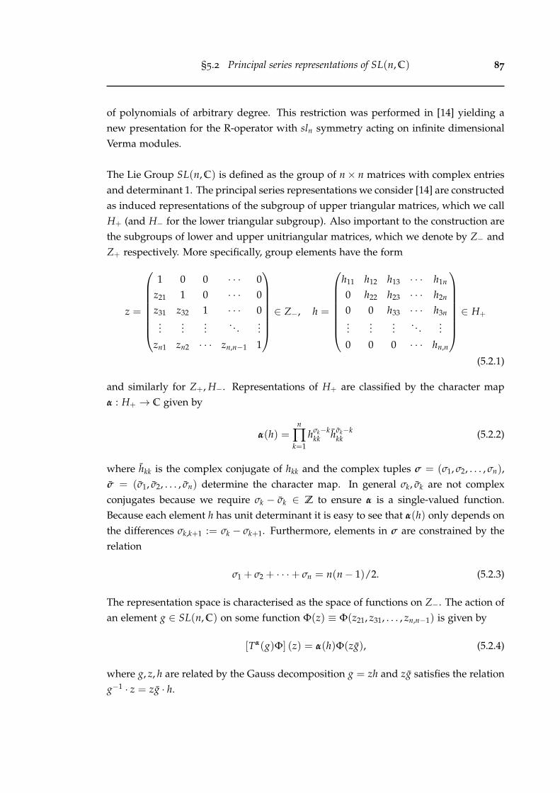
§5.2 Principal series representations of SL(n, C) 87
of polynomials of arbitrary degree. This restriction was performed in [14] yielding anew presentation for the R-operator with sln symmetry acting on infinite dimensionalVerma modules.
The Lie Group SL(n, C) is defined as the group of n× n matrices with complex entriesand determinant 1. The principal series representations we consider [14] are constructedas induced representations of the subgroup of upper triangular matrices, which we callH+ (and H− for the lower triangular subgroup). Also important to the construction arethe subgroups of lower and upper unitriangular matrices, which we denote by Z− andZ+ respectively. More specifically, group elements have the form
z =
1 0 0 · · · 0z21 1 0 · · · 0z31 z32 1 · · · 0...
......
. . ....
zn1 zn2 · · · zn,n−1 1
∈ Z−, h =
h11 h12 h13 · · · h1n
0 h22 h23 · · · h2n
0 0 h33 · · · h3n...
......
. . ....
0 0 0 · · · hn,n
∈ H+
(5.2.1)
and similarly for Z+, H−. Representations of H+ are classified by the character mapα : H+ → C given by
α(h) =n
∏k=1
hσk−kkk hσk−k
kk (5.2.2)
where hkk is the complex conjugate of hkk and the complex tuples σ = (σ1, σ2, . . . , σn),σ = (σ1, σ2, . . . , σn) determine the character map. In general σk, σk are not complexconjugates because we require σk − σk ∈ Z to ensure α is a single-valued function.Because each element h has unit determinant it is easy to see that α(h) only depends onthe differences σk,k+1 := σk − σk+1. Furthermore, elements in σ are constrained by therelation
σ1 + σ2 + · · ·+ σn = n(n− 1)/2. (5.2.3)
The representation space is characterised as the space of functions on Z−. The action ofan element g ∈ SL(n, C) on some function Φ(z) ≡ Φ(z21, z31, . . . , zn,n−1) is given by
[Tα(g)Φ] (z) = α(h)Φ(zg), (5.2.4)
where g, z, h are related by the Gauss decomposition g = zh and zg satisfies the relationg−1 · z = zg · h.

88 R-matrix factorisation by Q-operators
We are interested in a special case of representations known as the unitary principal seriesrepresentations. These are irreducible representations which parametrise σk,k+1, σk,k+1 by
σk,k+1 = −nk
2+ iλk, σk,k+1 =
nk
2+ iλk, nk ∈ Z, λk ∈ R. (5.2.5)
For these representations Tα(g) is a unitary operator on the Hilbert space L2(Z−) withinner product
〈Φ1|Φ2〉 =∫
∏1≤i≤k≤n
d2zki(Φ1(z))∗Φ2(z). (5.2.6)
The representation theory of SL(n, C) is closely related to that of the complex Lie al-gebra sln. Taking g ∈ SL(n, C) close to the identity 1 we write it as g = 1 + εE =
1 + ∑1≤i,k≤n εikEki where
(Eik)nm = δinδkm −1n
δikδnm (5.2.7)
are the generators of SL(n, C) in the fundamental representation. The operator Tα(g)then acts as[
Tα(1 + ∑1≤i,k≤n
εikEki)Φ
](z) = Φ(z) + ∑
1≤i,k≤n
(εikEki + εikEki
)Φ(z) +O(ε2). (5.2.8)
The linear operators Eik(Eik) acting on variables zmn(zmn) are generators of the Liealgebra sln. They satisfy the commutation relations
[Eik, Enm] = δknEim − δimEnk. (5.2.9)
They can be considered as the standard generators of the Lie algebra gln with the extrarelation ∑n
i=1 Eii = 0. This can be seen from their operator form given in [14] by
Eki = −∑mn
zim (Dnm + δnmσm)(
z−1)
nk, (5.2.10)
Dki =n
∑m=k
zmk∂
∂zmi= −
i
∑m=1
zim∂
∂zkmk > i (5.2.11)
where zki =(z−1)
ki , zii = 1 and operators Dnm are non-zero only for n > m. The op-erators (5.2.10) define a highest weight representation of sln acting on a Verma module
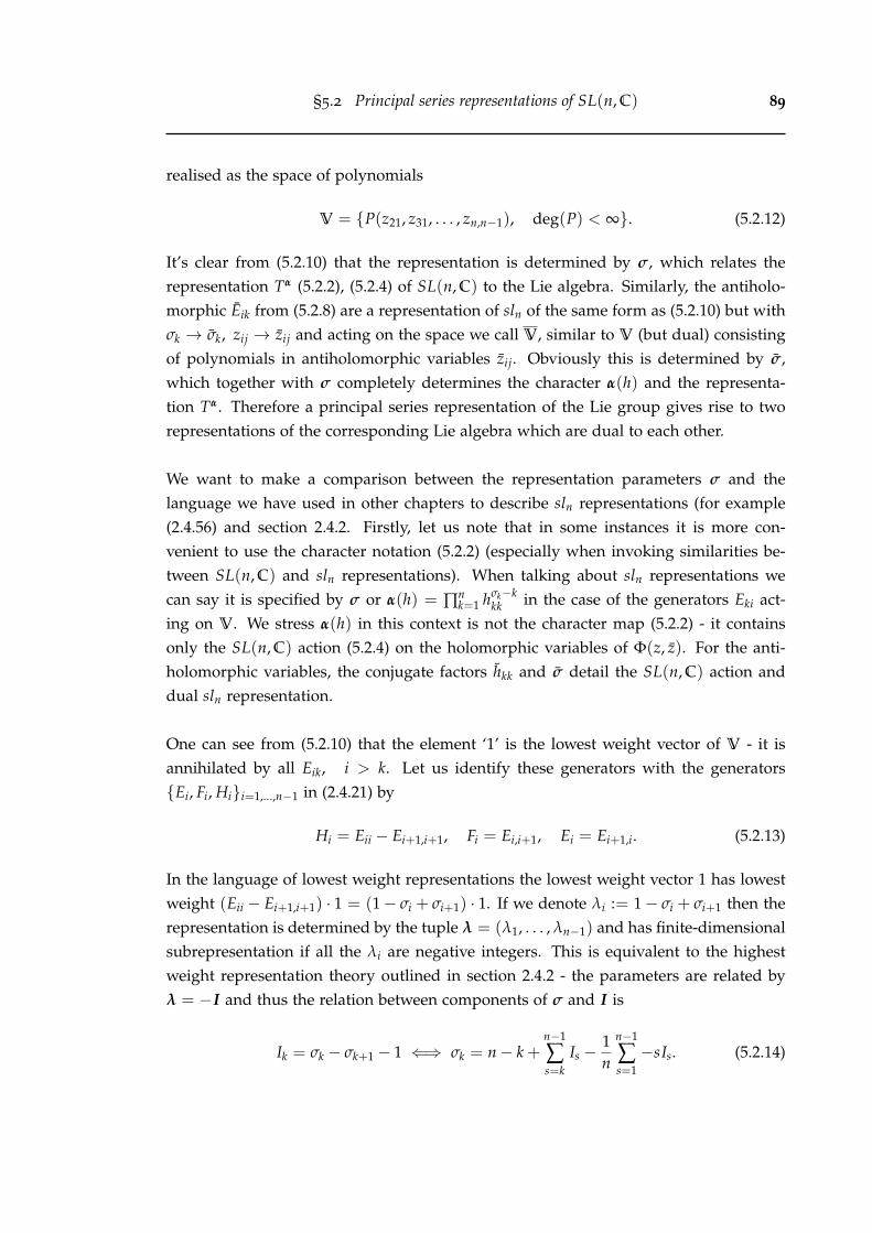
§5.2 Principal series representations of SL(n, C) 89
realised as the space of polynomials
V = P(z21, z31, . . . , zn,n−1), deg(P) < ∞. (5.2.12)
It’s clear from (5.2.10) that the representation is determined by σ, which relates therepresentation Tα (5.2.2), (5.2.4) of SL(n, C) to the Lie algebra. Similarly, the antiholo-morphic Eik from (5.2.8) are a representation of sln of the same form as (5.2.10) but withσk → σk, zij → zij and acting on the space we call V, similar to V (but dual) consistingof polynomials in antiholomorphic variables zij. Obviously this is determined by σ,which together with σ completely determines the character α(h) and the representa-tion Tα. Therefore a principal series representation of the Lie group gives rise to tworepresentations of the corresponding Lie algebra which are dual to each other.
We want to make a comparison between the representation parameters σ and thelanguage we have used in other chapters to describe sln representations (for example(2.4.56) and section 2.4.2. Firstly, let us note that in some instances it is more con-venient to use the character notation (5.2.2) (especially when invoking similarities be-tween SL(n, C) and sln representations). When talking about sln representations wecan say it is specified by σ or α(h) = ∏n
k=1 hσk−kkk in the case of the generators Eki act-
ing on V. We stress α(h) in this context is not the character map (5.2.2) - it containsonly the SL(n, C) action (5.2.4) on the holomorphic variables of Φ(z, z). For the anti-holomorphic variables, the conjugate factors hkk and σ detail the SL(n, C) action anddual sln representation.
One can see from (5.2.10) that the element ‘1’ is the lowest weight vector of V - it isannihilated by all Eik, i > k. Let us identify these generators with the generatorsEi, Fi, Hii=1,...,n−1 in (2.4.21) by
Hi = Eii − Ei+1,i+1, Fi = Ei,i+1, Ei = Ei+1,i. (5.2.13)
In the language of lowest weight representations the lowest weight vector 1 has lowestweight (Eii − Ei+1,i+1) · 1 = (1− σi + σi+1) · 1. If we denote λi := 1− σi + σi+1 then therepresentation is determined by the tuple λ = (λ1, . . . , λn−1) and has finite-dimensionalsubrepresentation if all the λi are negative integers. This is equivalent to the highestweight representation theory outlined in section 2.4.2 - the parameters are related byλ = −I and thus the relation between components of σ and I is
Ik = σk − σk+1 − 1 ⇐⇒ σk = n− k +n−1
∑s=k
Is −1n
n−1
∑s=1−sIs. (5.2.14)

90 R-matrix factorisation by Q-operators
In what follows we will mostly use the I parameters in the context of sln Verma modulesrather than σ (which we still use for SL(n, C)) in order to be consistent with otherchapters and to make comparisons easier.
5.3 Factorised form and properties
It was proven in [66] that the SL(n, C) invariant R-matrix acting on the tensor productof two unitary principal series representations Tα ⊗ Tβ has the factorised form
R12(u− v) = P12R(1)12 (u1 − v1) . . . R
(n)12 (un − vn), (5.3.1)
where u, v are spectral parameters and ui := u− σi, vi := v− ρi. The factors R(i)(λ)
solve (5.1.9) and are intertwiners of representations Tα ⊗ Tβ with Tαi,λ ⊗ Tβi,λ . That is,
R(i)(λ)(
Tα(g)⊗ Tβ(g))=(
Tαi,λ(g)⊗ Tβi,λ(g))
R(i)(λ) ∀g ∈ SL(n, C), (5.3.2)
αi,λ(h) = h−λii h−λ
ii α(h), βi,λ(h) = hλii h
λii β(h). (5.3.3)
As we will see, the intertwining action of the R(i) has to be carefully taken into accountwhen multiplying factors such as in (5.3.1) because the representation parameters of theoperator depend on its position in the product. We will sometimes write the operatoras R(i)(λ|σ′, ρ′) to indicate the transformed representation it acts as. Computing thetransforms (5.3.3) over all R(i) on the right hand side of (5.3.1) we see that the overallchange to the representation parameters is nil, as we would expect from the left handside.
The intertwiner factors are very interesting objects in their own right. Some non-trivialrelations they satisfy include
R(i)12 (0) = id, (5.3.4a)
R(i)12 (λ)R
(i)12 (µ) = R
(i)12 (λ + µ), (5.3.4b)
R(i)12 (λ)R
(j)23 (µ) = R
(j)23 (µ)R
(i)12 (λ), (5.3.4c)
R(i)12 (λ)R
(i)23 (λ + µ)R
(i)12 (µ) = R
(i)23 (µ)R
(i)12 (λ + µ)R
(i)23 (λ), (5.3.4d)
R(i)12 (λ− σi + ρi)R
(j)12 (λ− σj + ρj) = R
(j)12 (λ− σj + ρj)R
(i)12 (λ− σi + ρi). (5.3.4e)
Identity (5.3.4d) states that the factors satisfy a Yang-Baxter type equation, although theoperator composition à la (5.3.2) is more complicated. We already know from chapter 3

§5.4 Operator kernel and hermitian form 91
that at least for symmetric tensor representations the R-matrix factorises into ‘smaller’R-matrices without the difference property. We will aim to clarify the connection be-tween these factorisations. Equation (5.3.4e) states that the factors R(i)(ui− vi) commutewith each other.
The operators R(i) acting on the principal series representation space of SL(n, C) arerepresented in [66] as a product of even more elementary intertwining operators. Theaction of these elementary operators takes the form of an integral operator. We mayview the R-operators as being composed of even smaller building blocks. However,unlike R(i), these operators cannot be restricted to sln Verma modules. Therefore weshould be able to represent the operator R(i) restricted to Verma modules as a matrix,and calculate a formula for its entries. In principle, this could be done by evaluatingthe integral operator directly for monomial test functions but it appears to be simplerto write the action down in terms of the operator kernel with respect to a hermitianform on the Verma module.
5.4 Operator kernel and hermitian form
In this section we will present a construction of the factors R(i) operating on sln Vermamodules. It was first presented in [14], and we will follow it explicitly for the case ofsl2, sl3 to construct a matrix representation of the operators and a formula for theirelements.
Let us first give a brief overview of some concepts that we will use. A hermitianform Ω : V×V→ C can be specified in terms of a reproducing kernel. A reproducingkernel E(z, w) evaluates the point P(z) ∈ V through the hermitian form by
P(z) = Ω (E(z, α), P(α)) . (5.4.1)
Fixing a basis en(z) of V we can represent the hermitian form as a matrix withelements Ωnm(en, em). Expanding E(z, α) in this basis it is easy to see Ω−1 forms thecoefficients of this expansion. That is,
E(z, α) = ∑m,n
em(z)Ω−1mnen(α) (5.4.2)
Generally speaking, we associate an operator with a kernel and hermitian form (andvice versa) - the reproducing kernel being associated with the identity operator. Given

92 R-matrix factorisation by Q-operators
an arbitrary operator A acting on V we denote its kernel by A(z, w). The relationbetween an operator, its kernel and hermitian form is given by
[AP] (z) = Ω(A(z, α), P(α)), (5.4.3)
A(z, α) = ∑nm
en(z)(
AΩ−1)
nmem(α), (5.4.4)
of which (5.4.1) and (5.4.2) is a particular case.
We will construct the factors R(i) by first constructing their kernels and the associ-ated hermitian form, and then evaluating (5.4.3). We start from a special form for thereproducing kernel and kernels of the operators R(i). For a sln Verma module of highestweight I the reproducing kernel has the form [14]
E I(z, α) =n−1
∏k=1
(∆k(α†z))Ik , (5.4.5)
where ∆k(M) = Det(Mk) and Mk is the k-th main minor of the matrix M. The corre-sponding hermitian form will be denoted by ΩI . In this Verma module we will workwith the basis
ei(z) = ∏s>l
zislsl , (5.4.6)
indexed by the tuple i = (i21, . . . , in,n−1). We use the same notation for the second tensorfactor acted on by R(i) and denote its reproducing kernel by E J(w, β). The kernel ofR(i)(λ) is denoted by Rλ,I J(z, w|α, β). A presentation of this kernel was constructed in[14] by considering the operator action on the coherent state basis of principal seriesrepresentations. We begin with this presentation which, in the notation of [14], is givenby
R(i)λ,I J(z, w|α, β) = Ai
(βww−1zα−1
z
)λ
iiE I(z, α)E J(w, β). (5.4.7)
Here, given matrices z, w ∈ Z−, α†, β† ∈ Z+ as in (5.2.1) we form the decomposition
α†z = zαdz,ααz, β†w = wβdw,ββw (5.4.8)
where zα, wβ ∈ Z−, αz, βw ∈ Z+ and dz,α, dw,β are diagonal matrices. Ai is a constantfactor which for now we choose to be 1.

§5.5 Construction for sl2 93
The action of the factor R(i)(λ) on an element ψ(z, w) ∈ V⊗V can be written as[R(i)(λ)ψ
](z, w) = ΩI J
(R(i)
λ,I J(z, w|α, β), ψ(α, β))
. (5.4.9)
We recall that the variables α and β in R are conjugated with respect to the analo-gous variables in ψ - see (5.4.7), (5.4.8). The hermitian form ΩI J is constructed as thekronecker product of the forms ΩI , ΩJ .
5.5 Construction for sl2
In this section we will explicitly carry out the construction outlined in the last sectionfor the case of the Lie algebra sl2. That is, we want to construct the sl2 invariant R-matrix of the form (5.3.1). Here we will rewrite this equation for the case n = 2 withexplicit dependence on the spectral parameter λ and weight parameters I, J. That is,we want to calculate
R12(λ) = P12R(1)12 (λ +
J − I2| I + J
2− λ,
I + J2
+ λ)R(2)12 (λ +
I − J2|I, J). (5.5.1)
We will do this by first calculating the factors R(i)12 (λ|I, J) and then composing them
with the substituted variables. To do this, we must first calculate the kernels of theoperators involved.
Throughout we work with 2 × 2 matrices belonging to SL(2, C) and its subgroups(5.2.1). Note that the matrices in Z− are functions of only a single variable z21. There-fore we can drop the index and work with the variables z, w, α, β etc. Also the basis ofmonomials (5.4.6) is just the set zii≥0.
Using (5.4.5) the reproducing kernel may be written in the form
E I(z, α) = ∆1(α†z)I
= (1 + zα)I (5.5.2)
Using the binomial theorem to expand this in the monomial basis gives
E I(z, α) =∞
∑k=0
(−1)k(−I)k
k!αkzk. (5.5.3)

94 R-matrix factorisation by Q-operators
This terminates if and only if I ∈ Z+. Since αk and zk are our basis elements and weknow the reproducing kernel has the form (5.4.2), it is easy to see that Ω−1
I is given bya diagonal matrix. Therefore we deduce that the elements of ΩI are given by
[ΩI ]mn = δn,m(−1)n n!
(−I)n. (5.5.4)
Next we want to calculate the kernels R(1)λ,I J ,R
(2)λ,I J . First we need the decomposition
(5.4.8) for 2× 2 matrices. It is
α†z =
(1 + αz α
z 1
)
=
(1 0z
1+αz 1
)(1 + αz 0
0 11+αz
)(1 α
1+αz
0 1
)(5.5.5)
= zαdz,ααz
and similarly for β†w. We then calculate the matrix βww−1zα−1z in (5.4.7) to be
βww−1zα−1z =
(1 β
1+βw
0 1
)(1 0−w 1
)(1 0z 1
)(1 −α
1+αz
0 1
)
=
( 1+βz1+βw
β−α(1+αz)(1+βw)
z− w 1+αw1+αz
). (5.5.6)
Combining (5.5.2) and (5.5.6) we see that the kernels (5.4.7) in the case of sl2 can berepresented by the functions
R(1)λ,I J(z, w|α, β) = (1 + αz)I(1 + βw)J−λ(1 + βz)λ, (5.5.7a)
R(2)λ,I J(z, w|α, β) = (1 + αz)I−λ(1 + βw)J(1 + αw)λ. (5.5.7b)
We will calculate R(i)(λ) by comparing the coefficients in the expansions of (5.5.7) and(5.4.4). Extracting the elements of R(i)(λ) is easy because Ω is a diagonal matrix. Theseries expansion of the R(i)
λ,I J are given by
R(1)λ,I J(z, w|α, β) =
∞
∑s1,s2,s3=0
(−1)s1+s2+s3(−I)s1(λ− J)s2(−λ)s3
s1!s2!s3!zs1+s3 ws2 αs1 β
s2+s3 , (5.5.8a)
R(2)λ,I J(z, w|α, β) =
∞
∑s1,s2,s3=0
(−1)s1+s2+s3(λ− I)s1(−J)s2(−λ)s3
s1!s2!s3!zs1 ws2+s3 αs1+s3 β
s2 . (5.5.8b)

§5.5 Construction for sl2 95
Now comparing to (5.4.4),
R(k)λ,I J(z, w|α, β) =
∞
∑i,j,i′,j′=0
(−1)i′+j′[R(k)(λ|I, J)
]i′,j′
i,j
(−I)i′(−J)j′
i′!j′!ziwjαi′β
j′(5.5.9)
and one can see that (by equating coefficients) we must have
Proposition 5.5.1.
[R(1)(λ|I, J)
]i′,j′
i,j= δi+j,i′+j′
j′!(−λ)j′−j(λ− J)j
j!(−J)j′(j′ − j)!, (5.5.10a)[
R(2)(λ|I, J)]i′,j′
i,j= δi+j,i′+j′
i′!(−λ)i′−i(λ− I)i
i!(−I)i′(i′ − i)!. (5.5.10b)
The ice rule i + j = i′ + j′ enters by equating the exponents of (5.5.8) and (5.5.9). Imme-diately we see that both operators are defined by essentially the same function. Theyare related by a swapping of indices, that is
[R(1)(λ|I, J)
]i′,j′
i,j=[R(2)(λ|J, I)
]j′,i′
j,i. (5.5.11)
We can now calculate the R-matrix (5.5.1). Let us first explain the variable substitu-tions we need to make in more detail. As mentioned in the last section, the operatorsR(i)(λ) (factorising the SL(2, C)-invariant R-matrix) are intertwiners of principal seriesrepresentations - (5.3.2) and (5.3.3). This is still true in the restriction to Verma mod-ules. Using (5.3.3) it is easily to calculate how each factor transforms the representationparameters I, J. For convenience we write it down explicitly:
R(1)(λ)(
π I ⊗ π J)=(
π I+λ ⊗ π J−λ)
R(1)(λ), (5.5.12a)
R(2)(λ)(
π I ⊗ π J)=(
π I−λ ⊗ π J+λ)
R(2)(λ). (5.5.12b)
Consequently, the representation parameters of R(i)(λ|I, J) depend not only on the rep-resentation parameters of the operators preceding it but also the spectral parameters- a subtle detail. Given λ is generic, this means that R(i)(λ) generally maps an inte-gral highest weight representation to a non-integral one - it does not preserve finitedimensional subspaces in the Verma module acted upon by the R-matrix when I, J areintegers. So even though the R-operator can be restricted to finite representations forintegral weights, the multiplication of the operators comprising it is over an infinitedimensional space.

96 R-matrix factorisation by Q-operators
We can now write down a formula for elements of the R-matrix RI J(λ). Using theconstructed factors (5.5.10) we get
[R(λ)]i′,j′
i,j = ∑r,s
[R(1)(λ +
J − I2| I + J
2− λ,
I + J2
+ λ)
]r,s
j,i
[R(2)(λ +
I − J2|I, J)
]i′,j′
r,s
=(−I)ii′!(−I)i′ i!
i+j
∑r,s=0
δi+j,r+s,i′+j′s!(−λ + I
2 −J2 )j−r(−λ− I
2 +J2 )i′−r(λ− I
2 −J2 )r
r!(j− r)!(i′ − r)!(−λ− I2 −
J2 )s
(5.5.13)
Even though there are two summation indices this really only a single sum because ofthe kronecker delta function. We can use this relation to eliminate the sum over r or s;we choose s. We can see from the sum (5.5.13) that r runs from 0 to Min(i′, j) and socan safely make the substitution s = i + j− r without summing negative s values. As aresult we obtain the expression
[RI,J(λ)]i′,j′
i,j = δi+j,i′+j′(i + j)!(−I)i(−λ + I
2 −J2 )j(−λ + J
2 −I2 )i′
i!j!(−I)i′(−λ− I2 −
J2 )i+j
× 4F3
(−i′ −j λ− I
2 −J2 λ + I
2 +J2 − i− j + 1
−i− j λ + J2 −
I2 − j + 1 λ + I
2 −J2 − i′ + 1
∣∣∣∣∣ 1
), (5.5.14)
for elements of the sl2-invariant R-matrix acting on Verma modules V⊗V. They are
4F3 balanced and terminating hypergeometric series. It is very easy to compare thisformula with (3.7.7) obtained from the 3D model approach. They are the same up to aswapping of indices, that is
[RI,J(λ)]i′,j′
i,j =[
R(2),rJ,I (λ)
]j′,i′
j,i, (5.5.15)
but this is just the symmetry (3.7.21a) found using the 3-dimensional approach. Weconclude that we are dealing with the same R-matrix.
Actually, we can get (3.7.7) exactly from this chapter’s construction without havingto appeal to symmetry relations. It turns out the symmetry in this constructions mani-fests itself in the reordering of the factors (5.3.4e). Using this relation the R-matrix alsofactorises as
[R(λ)]i′,j′
i,j = ∑r,s
[R(2)(λ +
I − J2| I + J
2+ λ,
I + J2− λ)
]r,s
j,i
[R(1)(λ +
J − I2|I, J)
]i′,j′
r,s
=j′!(−J)j
j!(−J)j′
i+j
∑r,s=0
δi+j,r+s,i′+j′r!(−λ− I
2 +J2 )r−j(−λ + I
2 −J2 )r−i′(λ− I
2 −J2 )s
s!(r− i′)!(r− j)!(−λ− I2 −
J2 )r
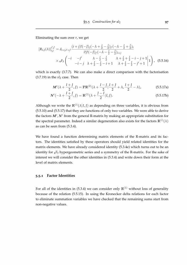
§5.5 Construction for sl2 97
Eliminating the sum over r, we get
[RI,J(λ)]i′,j′
i,j = δi+j,i′+j′(i + j)!(−J)j(−λ + I
2 −J2 )j′(−λ− I
2 +J2 )i
i!j!(−J)j′(−λ− I2 −
J2 )i+j
× 4F3
(−i −j′ λ− I
2 −J2 λ + I
2 +J2 − i− j + 1
−i− j λ + J2 −
I2 − i + 1 λ + I
2 −J2 − j′ + 1
∣∣∣∣∣ 1
), (5.5.16)
which is exactly (3.7.7). We can also make a direct comparison with the factorisation(3.7.19) in the sl2 case. Then
Mr(λ +I + J
2, J) = PR(2)(λ +
I − J2| I + J
2+ λ,
I + J2− λ), (5.5.17a)
Nr(−λ +I + J
2, J) = R(1)(λ +
J − I2|I, J). (5.5.17b)
Although we write the R(i)(λ|I, J) as depending on three variables, it is obvious from(5.5.10) and (5.5.17) that they are functions of only two variables. We were able to derivethe factors Mr, Nr from the general R-matrix by making an appropriate substitution forthe spectral parameter. Indeed a similar degeneration also exists for the factors R(i)(λ)
as can be seen from (5.3.4).
We have found a function determining matrix elements of the R-matrix and its fac-tors. The identities satisfied by these operators should yield related identities for thematrix elements. We have already considered identity (5.3.4e) which turns out to be anidentity for 4F3 hypergeometric series and a symmetry of the R-matrix. For the sake ofinterest we will consider the other identities in (5.3.4) and write down their form at thelevel of matrix elements.
5.5.1 Factor Identities
For all of the identities in (5.3.4) we can consider only R(1) without loss of generalitybecause of the relation (5.5.15). In using the Kronecker delta relations for each factorto eliminate summation variables we have checked that the remaining sums start fromnon-negative values.

98 R-matrix factorisation by Q-operators
Zero spectral parameter
The identity (5.3.4a) is obvious by inspecting (5.5.10). When λ = 0 the functions in(5.5.10) are zero unless j = j′, i = i′, in which case all terms in the numerator anddenominator cancel.
Yang-Baxter identity
The identity (5.3.4d) is a Yang-Baxter relation for the factors R(i)(λ). This relation is notsurprising given the link established by (5.5.17) between the factors R(i)(λ) and thosein (3.7.17). At the level of matrix elements, the Yang-Baxter equation for the factors isan identity for 4F3 hypergeometric series. In constructing the identity we will denotethe left hand side of (5.3.4d) by L and the right hand side by R. The identity can beexpressed as
[L(λ, µ)]i′,j′,k′
i,j,k = ∑r,l,s=0
[R
(1)12 (λ|I + µ, J + λ)
]r,l
i,j
[R
(1)23 (λ + µ|J − µ, K)
]s,k′
l,k
[R
(1)12 (µ|I, J)
]i′,j′
r,s,
[R(λ, µ)]i′,j′,k′
i,j,k = ∑r,l,s=0
[R
(1)23 (µ|J − µ, K− λ)
]r,l
j,k
[R
(1)12 (λ + µ|I, J + λ)
]i′,s
i,r
[R
(1)23 (λ|J, K)
]j′,k′
s,l.
There are 3 delta functions on each side implying the global conservation law i+ j+ k =
i′ + j′ + k′ as well as the bounds 0 ≤ s, l ≤ j′ + k′ and 0 ≤ r ≤ j + k on the summationindices. These bounds can be further refined by looking at the explicit expression. Wealso use the conservation laws to eliminate two summation variables on each side. Onthe left hand side we subsitute r = i′ + j′ − s, l = k′ − k + s and on the right handside l = j + k− r, s = r + i− i′. Simplifying some of the Pochhammer symbols in theresulting single sum, we obtain
[L(λ, µ)]i′,j′,k′
i,j,k = δi+j+k,i′+j′+k′ [A(λ, µ)]i′,j′,k′
i,j,k(−J)j(−λ− µ)k′−k(−µ)j′(−λ)k′−k−j
(−J)j′(−J − λ)k′−k(i− i′)!
×j′
∑s=0
(−j′, k′ − k + 1, µ− J, i− i′ − j′ − λ)s(1 + i− i′ − j′ + s)j′−s
s!(1 + µ− j′,−λ− J + k′ − k)s,
(5.5.18a)
[R(λ, µ)]i′,j′,k′
i,j,k = δi+j+k,i′+j′+k′ [A(λ, µ)]i′,j′,k′
i,j,k(−λ− µ)i−i′(−µ)j(−λ)i−i′−j′
(−J − λ)i−i′(k′ − k)!

§5.5 Construction for sl2 99
×j
∑r=0
(−j, 1 + i− i′, µ− J, k′ − k− j− λ)r(1 + k′ − k− j + r)j−r
r!(1 + µ− j,−λ− J + i− i′)r,
(5.5.18b)
[A(λ, µ)]i′,j′,k′
i,j,k =k′!(λ + µ− K)k
j!k!(−K)k′. (5.5.18c)
Both sides are given by balanced and terminating 4F3 hypergeometric series. In fact, wecan rewrite this identity so that is expresses a symmetry of the function for the elementson both sides. If we define L(λ, µ) and R(λ, µ) by multiplying the formulas for L(λ, µ)
and R(λ, µ) by (−J)j′ and then removing the A(λ, µ) term we obtain the symmetry
[R(λ, µ)
]i′,j′,k′
i,j,k =[R(λ, µ)
]k,j,ik′,j′,i′ . (5.5.19)
This identity is a combination of Whipple transformations (A.2.7) and the numeratorterm terminating the series is changed from j′ to j.
Additive spectral parameter identity
On the level of matrix elements we expect a summation formula, given the left handside contains a sum over matrix elements and the right hand side is just a product.Indeed, the identity reads
[LHS(λ, µ)]i′,j′
i,j =i+j
∑r,s=0
[R(1)(λ; I + µ, J − µ)
]r,s
i,j
[R(1)(µ; I, J)
]i′,j′
r,s, (5.5.20)
[RHS(λ, µ)]i′,j′
i,j =[R(1)(λ + µ)
]i′,j′
i,j. (5.5.21)
The delta functions present on the left hand side imply the conservation law i + j =
i′ + j′ consistent with the right hand side. Eliminating the sum over ‘r’ we get
[LHS(λ, µ)]i′,j′
i,j = δi+j,i′+j′(−1)j (−µ)j′(λ + µ− J)j
j!(−J)j′(1 + λ)j∑s=0
(−j′,−λ− j)s
(s− j)!(µ− j′ + 1)s, (5.5.22a)
[RHS(λ, µ)]i′,j′
i,j = δi+j,i′+j′j′!(−λ− µ)j′−j(λ + µ− J)j′
(−J)j′(j′ − j)!j!. (5.5.22b)
Both sides are zero whenever j′ < j. The sum on the left appears to be a terminating
3F2 series with j′ − j terms but actually it is a 2F1 series. To see this we reverse the order

100 R-matrix factorisation by Q-operators
of the summation by substituting s = j′ − s which gives
[LHS(λ, µ)]i′,j′
i,j = δi+j,i′+j′(−1)j+j′ (−µ)j′(λ + µ− J)j(−λ− j)j′ j′!j!(−J)j′(1 + λ)j(1 + µ− j′)j′(j′ − j)!
× 2F1
(j− j′ −µ
1 + λ + j− j′
∣∣∣∣∣ 1
). (5.5.23)
This is essentially the Gauss summation formula (A.2.2) up to a change of variables.
Commutativity identity
Identity (5.3.4c) does not give a non-trivial identity at the level of matrix elements be-cause both sides are the same product of binomials. Regardless, we will still write downthe elements for both sides of (5.3.4c). There are two orderings for the factors in thisidentity - R(1)R(2) and vice versa. For the former we have
[LHS(λ, µ)]i′,j′,k′
i,j,k = ∑s=0
[R
(1)12 (λ|I, J − µ)
]i′,s
i,j
[R
(2)23 (λ|J, K)
]j′,k′
s,k
= [RHS(λ, µ)]i′,j′,k′
i,j,k = ∑s=0
[R
(2)23 (µ|J − λ, K)
]s,k′
j,k
[R
(1)12 (λ|I, J)
]i′,j′
i,s
= δi+j+k,i′+j′+k′j′!(−λ)i−i′(−µ)k−k′(λ + µ− J)j
j!(i− i′)!(k− k′)!(−J)j′. (5.5.24)
On the left hand side we have made the substitution s = j′ + k′ − k and on the righthand side s = j + k − k′. The two delta functions in each factors also imply the deltafunction i + j + k = i′ + j′ + k′. For the other ordering we get
[LHS(λ, µ)]i′,j′,k′
i,j,k = ∑s=0
[R
(2)12 (λ|I, J + µ)
]i′,s
i,j
[R
(1)23 (λ|J, K)
]j′,k′
s,k
= [RHS(λ, µ)]i′,j′,k′
i,j,k = ∑s=0
[R
(1)23 (µ|J + λ, K)
]s,k′
j,k
[R
(2)12 (λ|I, J)
]i′,j′
i,s
= δi+j+k,i′+j′+k′i′!k′!(−λ)i′−i(−µ)k′−k(λ− I)i(µ− K)k
i!k!(i′ − i)!(k′ − k)!(−I)i′(−K)k′(5.5.25)
Even though we have written the identity as a sum over s there is actually no summationinvolved. This is easy to see from (5.5.10) because R(2) only depends on i indices andR(1) only depends on k indices. So both sides of the identity are just pure Kroneckerproducts of tensors.

§5.5 Construction for sl2 101
5.5.2 Discussion
In this section we have constructed the rational sl2 R-matrix at the level of matrix ele-ments using methods developed in [66; 14]. We have derived formulae for the R-matrixitself as well as its factors and related objects such as kernels and a hermitian form. Wehave also considered some identities satisfied by the factors and showed that they arecases of well known identities in theory of hypergeometric series.
What is interesting is that out of all the methods for constructing the sl2 R-matrix, thisone seems to be the most efficient. All of the other methods considered give a doubleor triple summation formulae for the matrix elements and much work has to be doneto simplify it to a single variable hypergeometric series. Of course, in this constructionwe only get a rational R-matrix and not the more general trigonometric R-matrix like inthe methods of spectral decomposition and the 3D model projection. However, it seemslike this construction should somehow generalise to trigonometric R-matrices, becausewe were able to construct a similar factorisation (3.5.6) from factors that are very similarto the ones constructed in this section.
We notice that there is a factorisation of the sl2 R-matrix and also its trigonometricand elliptic deformations in [67] in terms of ‘parameter permutation’ operators. Theseoperators can be combined to construct the factors R(i)(λ) and suggests that the finerstructure of the R-matrix discussed in this chapter splits even further. It would inter-esting to investigate this factorisation, which may offer another means of constructing(5.5.10), (3.5.6) and their elliptic generalisation. Another factorised form of the R-matrixrelated to the quantum modular double was constructed in [12] which is a combinationof two Uq(sl2) algebras but it is not clear how it can be restricted to Uq(sl2) or evenif the factorisation is similar to what we have found. It would be an interesting ex-ercise to reverse the arguments starting from the trigonometric R-matrix to derive theq-deformation of all the objects in this section. This is something we may attempt in thefuture.
Another appealing feature of the construction in this section is that we can constructthe factors from the ‘ground up’. The other means of deriving them, as in section 3.5,is to start with the general higher spin R-matrix and make the appropriate subsitutionto see it ‘degenerate’ into the desired factor. The general R-matrix is a far more com-plicated object than its factors and so this is not always feasible. We are very interestedin these factors as standalone objects. The function describing their elements appears

102 R-matrix factorisation by Q-operators
to be the same function appearing in other related studies. Firstly, they describe moreelementary R-matrices without difference property which as shown can be combinedto construct the general R-matrix. Secondly, with some small modifications [14] theydescribe a local form of the Q-operator. That is why we have named this chapter ‘Fac-torisation by Q-operators’. The Q-operators are known to factorise the transfer matrixthrough what is known as the fundamental fusion relation, but this is a factorisation ofglobal operators. The factorisation in this chapter seems to be a local form of this well-known relation and hence details another connection between an integrable model andits Q-operators.
Thirdly, and unexpectedly, the factors in this section are essentially the stochastic ma-trices that appear in the study of TASEP models [61; 22]. We study this aspect of thefactors in greater detail in chapter 8 but in summary the function determining elementsof R(1) and R(2) is a special case of the more general Φ function (8.0.4) which, as itturns out, factorises the general Uq(sln) R-matrix for symmetric tensor representations(8.0.10). However, it seems that this might be just a happy coincidence for sl2, and forgeneral n the correspondence is more complicated and maybe non-existent. In the nextsection we will see how these factors generalise in the case of sl3.
5.6 Construction for sl3
In this section we will repeat the steps of the last section but this time for the sl3invariant R-matrix acting on V ⊗V under arbitrary highest weight representationsπI ⊗ π J ∼= π(I1,I2) ⊗ π(J1,J2). In one way this construction gives a more general R-matrixthan (3.3.24) derived using the 3D approach which is only for symmetric tensor repre-sentations π(I,0)⊗π(J,0) but as mentioned multiple times in this chapter in another wayit is less general because it is a construction for the Lie algebra/rational R-matrices andnot the quantum group/trigonometric R-matrices.
In this case the R-matrix factorises into three factors of the form (5.3.1). The fac-tors with explicit dependence on spectral and weight parameters can be written asR(i)(λ|I1, I2; J1, J2) like for the sl2 case but expressions quickly become cumbersome sowe will refrain unless necessary. Instead we write it as
RI,J(λ) = PR(1)(λ1|I′′; J′′)R(2)(λ2|I
′; J′)R(3)(λ3|I; J) (5.6.1)

§5.6 Construction for sl3 103
where
λ1 =2J1 + J2 − 2I1 − I2
3, λ2 =
I1 − I2 + J2 − J1
3, λ3 =
2I2 + I1 − J2 − J1
3,
I ′ = (I1,−λ +I2 − I1 + J1 + 2J2
3), J′ = (J1, λ +
I1 + 2I2 − J1 + J2
3),
I ′′ = (−λ +2I1 + I2 + J1 − J2
3, J2), J′′ = (λ +
I1 − I2 + 2J1 + J2
3, I2). (5.6.2)
We now work with the group of 3× 3 matrices SL(3, C) and its subgroups (5.2.1). Thesubgroup Z− is a function of 3 variables z21, z31, z32, which for convenience we will re-label as z1, z2 and z3 respectively. We relabel the variables w, α and β in the same way.The basis of monomials (5.4.6) is the set zi := zi1
1 zi22 zi3
3 i1,i2,i3=0,... and similarly for theother variables. We also define zX := z1z3 − z2 to simplify some of our expressions.
The reproducing kernel (5.4.5) now has the form
E I(z, α) = ∆1(α†z)I1 ∆2(α
†z)I2
= (1 + z1α1 + z2α2)I1(1 + z3α3 + (z1z3 − z2)(α1α3 − α2))
I2 . (5.6.3)
We expand this out using the multinomial theorem
(1 + a2 + · · ·+ an)m = ∑
s2,...,sn
Dms2,...,sm
n
∏i=2
asii , (5.6.4a)
Dms2,...,sm
= (−1)s2+···+sm(−m)s2+···+sn
∏ni=2 si!
, (5.6.4b)
to get
E I(z, α) =∞
∑s,l=0
(−I2)l1+l2+l3+l4+l5l1!l2!l3!l4!l5!
(−1)s1+s2+l1+l3+l5
× zs1+l4+l51 zs2+l1+l2
2 zl3+l4+l53 α1
s1+l2+l5 α2s2+l1+l4 α3
l2+l3+l5 . (5.6.5)
To extract matrix elements out of this we must set
i1 = s1 + l4 + l5, i2 = s2 + l1 + l2, i3 = l3 + l4 + l5,
i′1 = s1 + l2 + l5, i′2 = s2 + l1 + l4, i′3 = l2 + l3 + l5.
In doing so we notice the conservation laws
i2 + i3 = i′2 + i′3, i1 + i′3 = i′1 + i3, i1 + i2 = i′1 + i′2

104 R-matrix factorisation by Q-operators
although the second relation is dependent on the other two. We find that the formulafor the matrix elements of the inverse hermitian form Ω−1
I1,I2is given by
[Ω−1
I1,I2
]i′1,i′2,i′3
i1,i2,i3= δi1+i2,i′1+i′2
δi2+i3,i′2+i′3(−1)i1+i2+i3−i′1 ∑
s1,s2,l1=0
(−I1)s1+s2(−I2)i2+i3−s2
s1!s2!l1!
× (−1)s1
(i2 − s2 − l1)!(s1 + i3 − i1)!(i1 + i2 − s2 − l1 − i′1)!(l1 + i′1 + s2 − s1 − i2)!
This is a triple sum expression for the matrix elements and is somewhat complicated.However, it can be summed up twice to obtain a single sum 4F3 hypergeometric series.That is, it can be simplified to
[Ω−1
I1,I2
]i′1,i′2,i′3
i1,i2,i3= δi1+i2,i′1+i′2
δi2+i3,i′2+i′3
(−1)i1+i′1 I2!(I1 + I2 − i′1 − i3)!(i3 + i′1)!i1!i3!i′1!i′3!(I1 + I2 − i2 − i3)!(i2 − i′1)!(I2 − i3 − i′1)!
×i1
∑s=0
(−i1,−i′1, i1 + i2 − i3 − i′1 − I1, I1 + I2 − i3 − i′1 + 1)s
s!(1 + i2 − i′1,−i3 − i′1, I2 − i3 − i′1 + 1)s. (5.6.6)
The hypergeometric series is balanced and terminating and the output contains notonly binomial terms but also polynomial factors in I1, I2. It is a far more complicatedexpression than what was found in the sl2 case (5.5.3) in not just the number of termsbut also because it is not a diagonal matrix. Calculating a formula for the inverse there-fore is non-trivial. However we were able to do it by making a few key observations.First, (5.6.6) can be evaluated for abstract I1, I2 because they do not enter the product ar-gument of pochhammer sumber. Second, the two conservation laws of Ω−1 imply thatthe matrix has a block diagonal form, indexed by the value of each conserved quantity.Each block is finite and restricting to each one we can calculate the inverse of the block- giving elements of Ω. Third, by inspection we notice that the polynomial factors inthese elements are almost exactly the same as Ω−1 except shifted by I1 → I1 + 1. Mak-ing this shift we see the difference between Ω and Ω−1 is just a product of binomialterms which are not difficult to work out. We find matrix elements of Ω are given bythe formula
[ΩI1,I2 ]i′1,i′2,i′3i1,i2,i3
= (−1)i′2+i3 δi1+i2,i′1+i′2δi2+i3,i′2+i′3
×i2!(i1 + i2 − i′1)!(i3 + i′1)!(−I1 + i1 − i3 − 1)i2−i′1
(i2 + i3 − I2 − i′2)i1
(i2 − i′1)!(−I1)i1+i2(−I1 − I2 − 1)i1+i2(−I2)i3
×i1
∑s=0
(−i1,−i′1, i1 + i2 − i3 − j1 − I1 − 1, I1 + I2 − j1 − i3 + 2)s
s!(1 + i2 − j1,−i3 − j1, 1 + I2 − i3 − j1)s. (5.6.7)

§5.6 Construction for sl3 105
The fact that Ω−1 is not diagonal also means we cannot use a shortcut that we usedin calculating the factors for sl2, where instead of finding matrix elements by consid-ering the action (5.4.9) we were able to separate them from the hermitian form in (5.4.4).
To calculate the kernels R(1),R(2),R(3) we first need to calculate the decomposition(5.4.8) for 3× 3 matrices. It is given by
α†z =
1 + z1α1 + z2α2 z3α2 + α1 α2
z2α3 + z1 1 + z3α3 α3
z2 z3 1
=
1 0 0z1+z2α3
1+z1α1+z2α21 0
z21+z1α1+z2α2
z3+zXα11+z3α3+zXαX
1
×
1 + z1α1 + z2α2 0 00 1+z3α3+zXαX
1+z1α1+z2α20
0 0 11+z3α3+zXαX
1 α1+z3α2
1+z1α1+z2α2
α21+z1α1+z2α2
0 1 α3+z1αX1+z3α3+zXαX
0 0 1
= zαdz,ααz (5.6.8)
and similarly for β†w. The matrix βww−1zα−1z is easy to calculate but the elements are
large expressions that are messy to write down. Since we are only interested in thediagonal elements for calculating the kernels we will just list those. They are
(βww−1zα−1
z
)11
=1 + z1β1 + z2β2
1 + w1β1 + w2β2,(
βww−1zα−1z
)22
=[1 + z3β3 + (w1 + w2β3)(α1 + z3α2) + zX βX(w1α1 + w2α2)
+zXαX + wX βX + zXα1(β3 − α3) + w1βX(z3 − w3)]
× (1 + z1α1 + z2α2)−1(1 + w3β3 + wX βX)
−1,(βww−1zα−1
z
)33
=1 + w3α3 + wXαX
1 + z3α3 + zXαX.
We use these to calculate the kernel functions R(i) from (5.4.7). They are
R(1)λ,I J(z, w|α, β) = (1 + z1β1 + z2β2)
λ(1 + z1α1 + z2α2)I1(1 + w1β1 + w2β2)
J1−λ
× (1 + z3α3 + zXαX)I2(1 + w3β3 + wX βX)
J2 (5.6.9a)
R(2)λ,I J(z, w|α, β) =
[1 + z3β3 + (w1 + w2β3)(α1 + z3α2) + zXαX + zX βX(w1α1 + w2α2)
+wX βX + zXα1(β3 − α3) + w1βX(z3 − w3)]λ
(1 + z1α1 + z2α2)I1−λ
× (1 + z3α3 + zXαX)I2(1 + w21β1 + w2β2)
J1(1 + w3β3 + wX βX)J2−λ
(5.6.9b)
R(3)λ,I J(z, w|α, β) = (1 + w3α3 + wXαX)
λ(1 + z1α1 + z2α2)I1(1 + w1β1 + w2β2)
J1
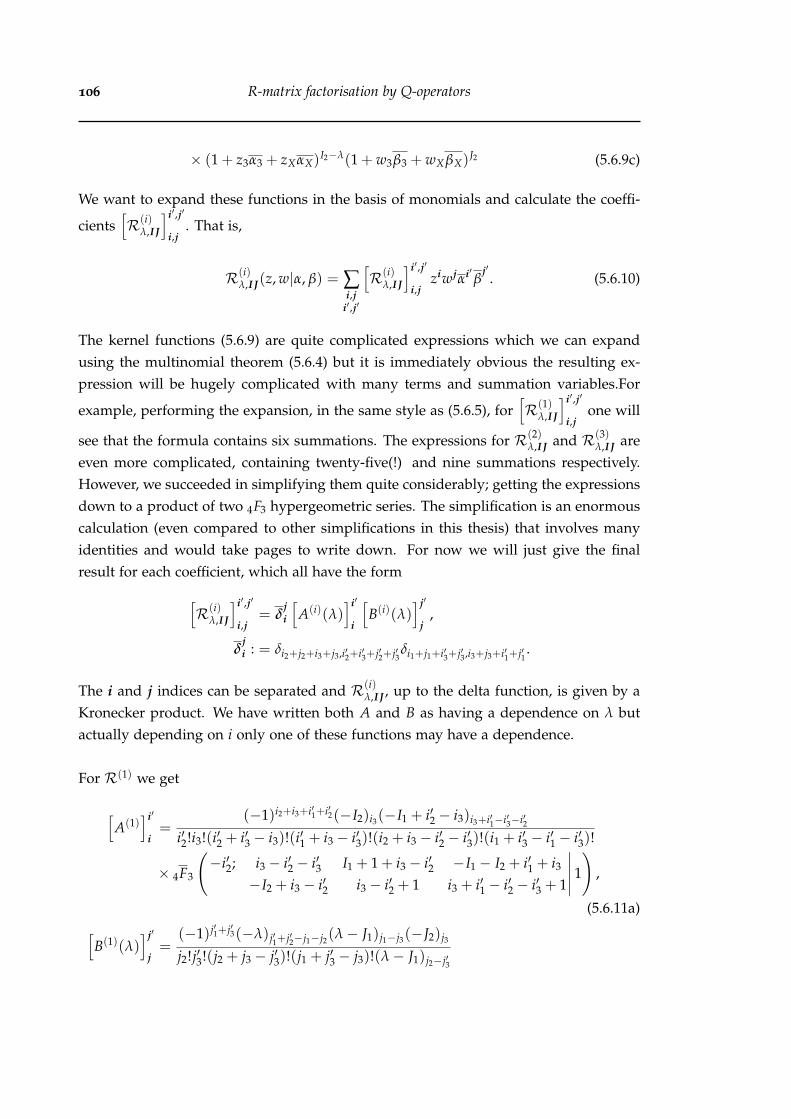
106 R-matrix factorisation by Q-operators
× (1 + z3α3 + zXαX)I2−λ(1 + w3β3 + wX βX)
J2 (5.6.9c)
We want to expand these functions in the basis of monomials and calculate the coeffi-
cients[R(i)
λ,I J
]i′,j′
i,j. That is,
R(i)λ,I J(z, w|α, β) = ∑
i,ji′,j′
[R(i)
λ,I J
]i′,j′
i,jziwjαi′β
j′. (5.6.10)
The kernel functions (5.6.9) are quite complicated expressions which we can expandusing the multinomial theorem (5.6.4) but it is immediately obvious the resulting ex-pression will be hugely complicated with many terms and summation variables.For
example, performing the expansion, in the same style as (5.6.5), for[R(1)
λ,I J
]i′,j′
i,jone will
see that the formula contains six summations. The expressions for R(2)λ,I J and R(3)
λ,I J areeven more complicated, containing twenty-five(!) and nine summations respectively.However, we succeeded in simplifying them quite considerably; getting the expressionsdown to a product of two 4F3 hypergeometric series. The simplification is an enormouscalculation (even compared to other simplifications in this thesis) that involves manyidentities and would take pages to write down. For now we will just give the finalresult for each coefficient, which all have the form[
R(i)λ,I J
]i′,j′
i,j= δ
ji
[A(i)(λ)
]i′
i
[B(i)(λ)
]j′
j,
δji : = δi2+j2+i3+j3,i′2+i′3+j′2+j′3
δi1+j1+i′3+j′3,i3+j3+i′1+j′1.
The i and j indices can be separated and R(i)λ,I J , up to the delta function, is given by a
Kronecker product. We have written both A and B as having a dependence on λ butactually depending on i only one of these functions may have a dependence.
For R(1) we get
[A(1)
]i′
i=
(−1)i2+i3+i′1+i′2(−I2)i3(−I1 + i′2 − i3)i3+i′1−i′3−i′2i′2!i3!(i′2 + i′3 − i3)!(i′1 + i3 − i′3)!(i2 + i3 − i′2 − i′3)!(i1 + i′3 − i′1 − i′3)!
× 4F3
(−i′2; i3 − i′2 − i′3 I1 + 1 + i3 − i′2 −I1 − I2 + i′1 + i3
−I2 + i3 − i′2 i3 − i′2 + 1 i3 + i′1 − i′2 − i′3 + 1
∣∣∣∣∣ 1
),
(5.6.11a)[B(1)(λ)
]j′
j=
(−1)j′1+j′3(−λ)j′1+j′2−j1−j2(λ− J1)j1−j3(−J2)j3
j2!j′3!(j2 + j3 − j′3)!(j1 + j′3 − j3)!(λ− J1)j2−j′3

§5.6 Construction for sl3 107
× 4F3
(−j2; j′3 − j3 − j2 λ− J1 − J2 + j1 + j′3 −λ + J1 + 1 + j′3 − j2
1 + j′3 − j2 1 + j1 + j′3 − j2 − j3 −J2 + j′3 − j2
∣∣∣∣∣ 1
).
(5.6.11b)
Note that we have written them in terms of regularised hypergeometric functions ac-cording to (A.1.4). Both formulae are balanced and terminating hypergeometric seriesand can be transformed using (the regularised version of) the Whipple identity (A.2.7).Now for R(2) we get
[A(2)(λ)
]i′
i=
(−1)i1+i2+i′1+i′3(−λ)i3+i′1−i′3−i1(−I2)i′3(−I1 − I2 + i3 + i′1)i2−i′1
(−λ− I2)i3
i1!i2!i′1!i′3!(i′1 + i′2 − i1 − i2)!(i2 + i3 − i′2 − i′3)!(−λ− I2)i3+i′1−i1
× 4F3
(−i′1; I1 + I2 + 1− i′1 − i′2 I1 + I2 + 1− i31 λ + I2 + 1 + i1 − i31
I1 + I2 + 2− i′1 I1 + I2 + 1− i2 − i31 λ + I2 + 1− i31
∣∣∣∣∣ 1
),
(5.6.12a)[B(2)(λ)
]j′
j=
(−1)j3+j′2(λ− J2)j3(−J2)j′3(−J1 − J2)j′2+j′3
j1!j3!j′1!j′2!(−J2)j′3+j1−j′1(−J1 − J2)j1+j′3
× 4F3
(−j1; J1 + J2 + 1− j1 − j2 J1 + J2 + 1− j1 − j′3 J2 + 1 + j′1 − j1 − j′3
J1 + J2 + 2− j1 J1 + J2 + 1− j1 − j′2 − j′3 J2 + 1− j1 − j′3
∣∣∣∣∣ 1
)(5.6.12b)
where we have defined i31 := i3 + i′1 for compactness. Both formulae are terminatinghypergeometric series but in general they are not balanced - A(2)(λ) is (1 + i′1 + i′2 −i1− i2)-balanced while B(2)(λ) is (1+ j1 + j2− j′1− j′2)-balanced. Finally for R(3) we get
[A(3)(λ)
]i′
i=
(−1)i1+i2+i3+i′1(−λ)i′2+i′3−i2−i3(λ− I2)i3(λ− I1 − I2 + i3 − i′1)i2−i′1i1!i2!i′1!(i3 + i′1 − i1)!(i′1 + i′2 − i1 − i2)!(i1 + i′3 − i′1 − i3)!
× 4F3
(−i′1; i1 − i′1 − i3 −λ + I1 + I2 + 1− i′1 − i3 I1 − i′1 − i′2
−i′1 − i3 −λ + I1 + I2 + 1− i2 − i3 − i′1 I1 + 1− i′1
∣∣∣∣∣ 1
), (5.6.13a)
[B(3)
]j′
j=
(−1)j1+j2+j3+j′1(−J2)j3(−J1 − J2)j′2+j′3j1!j′1!j′2!(j′3 + j1 − j′1)!(−J1 − J2)j1+j′3
× 4F3
(−j1; j′1 − j1 − j′3 J1 + J2 + 1− j1 − j′3 J1 − j1 − j2
−j1 − j′3 J1 + J2 + 1− j1 − j′2 − j′3 J1 + 1− j1
∣∣∣∣∣ 1
). (5.6.13b)
Just like (5.6.12) these formulae contain terminating hypergeometric series that are notbalanced - A(3)(λ) is (1+ i′1 + i′2− i1− i2)-balanced while B(3)(λ) is (1+ j1 + j2− j′1− j′2)-balanced.

108 R-matrix factorisation by Q-operators
Now we can calculate the factors R(i)(λ) by combining (5.6.11)-(5.6.13) and (5.6.7) in(5.4.9). We will calculate a formula for the matrix elements by considering the actionon the monomial basis zi′wj′, that is,
R(i)(λ) · zi′wj′ = ΩI J
(R(i)
λ,I J(z, w|α, β), αi′βj′)
,
= ∑ijsr
[Rλ,I J ]s,ri,j [ΩI J ]
i′,j′s,r ziwj, (5.6.14a)
= ∑ij
[R(i)(λ)
]i′,j′
i,jziwj. (5.6.14b)
All that is left is to calculate this expression. This is also an enormous calculationsimilar to what is required in obtaining (5.6.11)-(5.6.13). The steps are exhaustivelylong involving summing up the expression many times. There is a summation over 6indices (5.6.14a) with each element of R and ΩI J given by double sums. However, weutilise one observation that simplifies the calculations a great deal; the i and j indicesin formulae for R and ΩI J can be separated. This means we can split to simplificationinto two smaller computations. Perhaps a more efficient means of summing up andobtaining our final result exists but is unknown to us at this point.

§5.6 Construction for sl3 109
5.6.1 The factor R(1)(λ)
The final result of the calculation (5.6.14a) is the formula
Proposition 5.6.1.
[R(1)(λ)
]i′,j′
i,j=
δjiδi3,i′3
j′1!(j′2 + j′3)!(−J1 − 1)j′2(−λ + J1 + 1)j3(λ− J1)j1−j3(−λ)j′1+j′2−j1+j3
j1!j2!j3!(j′2 + j′3 − j2 − j3)!(j′1 − j1 − j′3 + j3)!(−J1)j′1+j′2(−J1 − J2 − 1)j′2+j′3
×j2+j3
∑m,l=0
(−j3, λ− J1 + j1 − j3, λ− J1 − J2 − 1)m(−j′2, J1 + 1− j′1 − j′2, J1 + J2 + 2− j′2 − j′3)l
m!(−j2 − j3, λ− J1 − j3)ml!(J1 + 2− j′2,−j′2 − j′3)l
× (−1)j2+j′3(−j2 − j3)l+m
(λ + 1 + j1 − j3 − j′1 − j′2)l+m(5.6.15)
for the matrix elements of R(1)(λ) in the case of sl3. This expression does not dependon the i indices (except for the delta functions) just like the sl2 case. It is a somewhatmore complicated expression than the sl2 given it is a double sum compared to a sim-ple product. In each summation variable the summation is a terminating 4F3 series thatis not balanced. It is interesting to analyse this formula by finding certain argumentswhere the expression simplifies.
One immediately sees from the denominator terms that the expression is trivially zerowhenever
j1 − j′1 > j3 − j′3 > j′2 − j2.
It reduces to a simpler expression whenever j3 = 0. In this case the summation in ‘m’disappears and we can rewrite the expression as the single sum
[R(1)(λ)
]i′,j′
i,j
∣∣∣∣j3=0
=δ
jiδi3,i′3
(−1)j2+j′3 j′1!(j′2 + j′3)!(−J1 − 1)j′2(λ− J1)j1(−λ)j′1+j′2−j1
j1!j2!(j′2 − j2 + j′3)!(j′1 − j1 − j′3)!(−J1)j′1+j′2(−J1 − J2 − 1)j′2+j′3
× 4F3
(−j′2 −j2 J1 + 1− j′1 − j′2 J1 + J2 + 2− j′2 − j′3
−j′2 − j′3 J1 + 2− j′2 λ + 1 + j1 − j′1 − j′2
∣∣∣∣∣ 1
).
Actually, if we instead set j′3, J2 = 0 we get a reduction to a product expression. To seethis, notice that the sum in ‘l’ becomes a 2F1 series and can be summed using the Gaussidentity (A.2.2).
The resultant formula still contains the summation in ‘m’ but this is now reduced to

110 R-matrix factorisation by Q-operators
a 2F1 series which can be summed up as well. The result is the product
[R(1)(λ)
]i′,j′
i,j
∣∣∣∣J2,j′3=0
=δ
jiδi3,i′3
j′1!j′2!(λ− J1)j1+j2(−λ)j′1+j′2−j1−j2
j1!j2!(−j′3)!j′3!(j3 + j′1 − j1)!(j′2 − j2 − j3)!(−J1)j′1+j′2
. (5.6.16)
Immediately we see that we must also have j3 = 0. So really, the resulting expression is
[R(1)(λ)
]i′,j′
i,j
∣∣∣∣J2,j3,j′3=0
= δjiδi3,i′3
j′1!j′2!(λ− J1)j1+j2(−λ)j′1+j′2−j1−j2
j1!j2!(j′1 − j1)!(j′2 − j2)!(−J1)j′1+j′2
. (5.6.17)
This formula is almost exactly the same as that which appears in the factorisation(3.7.18). Indeed, we already made the connection to Nr(I, J) in the case of sl2 by therelation (5.5.17b) and it seems that the same relation holds for sl3 when the secondrepresentation parameter J2 and indices j3, j′3 are ‘switched off’. Indeed,
Nr(−µ +I + J
2, J) = R(1)(µ +
J − I2|I, J1, 0)
∣∣∣∣j3,j′3=0
. (5.6.18)
This makes sense, the factor Nr(I, J) is a factor of sl3 R-matrix only for symmetrictensor representations and R(1)(λ) as we have constructed it (5.6.15) is a more generalobject - holding for all highest weight representations. The questions still remains:how does Mr(I, J) appear? For sl2 we could identify it with R(2)(λ) but now there aretwo factors which should somehow reduce to it in the restriction to symmetric tensorrepresentations.
5.6.2 The factor R(2)(λ)
The final result of the calculation (5.6.14a) is the formula
Proposition 5.6.2.
[R(2)(λ)
]i′,j′
i,j=
δji i′2!j′3!(−I1 + i3 − i′3)i2(−λ + i3 − i′3 − i1)i1(−λ)i3−i′3+i′1−i1(λ− J2)j3
(−1)j1+i′1+j′1+i2+i′2(i1, i2, j3, i2 + i3 − i′2 − i′3, j1 − j′1, j2 − j′2)!(−I1)i′2(−J2)j′3
× 4F3
(−i′1 −I1 − 1 −I1 + i2 + i3 − i′3 −λ + i3 − i′3
−I1 + i′2 −I1 + i3 − i′3 −λ + i3 − i′3 − i1
∣∣∣∣∣ 1
). (5.6.19)
This is a terminating (1 + i′1 + i′2 − i1 − i2)-balanced 4F3 hypergeometric series formulafor the matrix elements. This is a simpler expression than the one obtained for R(1)(λ)
and so it appears the relation (5.5.15) is broken for rank greater than 2. Another inter-
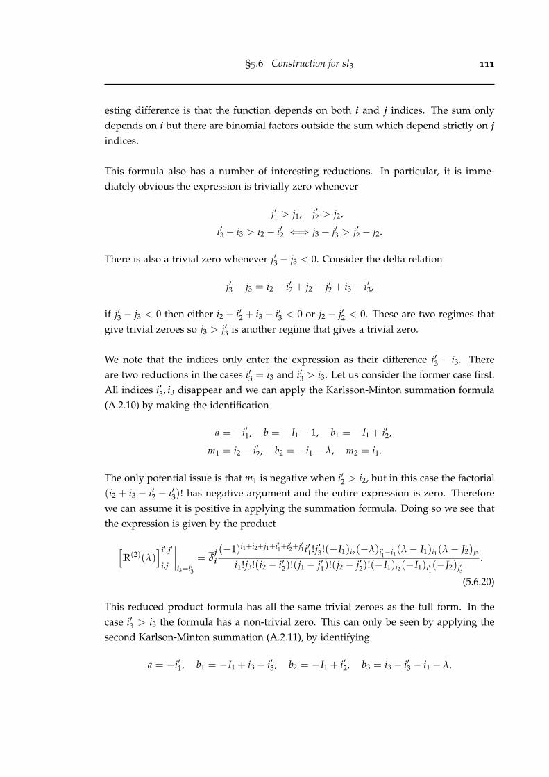
§5.6 Construction for sl3 111
esting difference is that the function depends on both i and j indices. The sum onlydepends on i but there are binomial factors outside the sum which depend strictly on jindices.
This formula also has a number of interesting reductions. In particular, it is imme-diately obvious the expression is trivially zero whenever
j′1 > j1, j′2 > j2,
i′3 − i3 > i2 − i′2 ⇐⇒ j3 − j′3 > j′2 − j2.
There is also a trivial zero whenever j′3 − j3 < 0. Consider the delta relation
j′3 − j3 = i2 − i′2 + j2 − j′2 + i3 − i′3,
if j′3 − j3 < 0 then either i2 − i′2 + i3 − i′3 < 0 or j2 − j′2 < 0. These are two regimes thatgive trivial zeroes so j3 > j′3 is another regime that gives a trivial zero.
We note that the indices only enter the expression as their difference i′3 − i3. Thereare two reductions in the cases i′3 = i3 and i′3 > i3. Let us consider the former case first.All indices i′3, i3 disappear and we can apply the Karlsson-Minton summation formula(A.2.10) by making the identification
a = −i′1, b = −I1 − 1, b1 = −I1 + i′2,
m1 = i2 − i′2, b2 = −i1 − λ, m2 = i1.
The only potential issue is that m1 is negative when i′2 > i2, but in this case the factorial(i2 + i3 − i′2 − i′3)! has negative argument and the entire expression is zero. Thereforewe can assume it is positive in applying the summation formula. Doing so we see thatthe expression is given by the product
[R(2)(λ)
]i′,j′
i,j
∣∣∣∣i3=i′3
= δji(−1)i1+i2+j1+i′1+i′2+j′1 i′1!j′3!(−I1)i2(−λ)i′1−i1(λ− I1)i1(λ− J2)j3
i1!j3!(i2 − i′2)!(j1 − j′1)!(j2 − j′2)!(−I1)i2(−I1)i′1(−J2)j′3
.
(5.6.20)
This reduced product formula has all the same trivial zeroes as the full form. In thecase i′3 > i3 the formula has a non-trivial zero. This can only be seen by applying thesecond Karlson-Minton summation (A.2.11), by identifying
a = −i′1, b1 = −I1 + i3 − i′3, b2 = −I1 + i′2, b3 = i3 − i′3 − i1 − λ,

112 R-matrix factorisation by Q-operators
m1 = i′3 − i3 − 1, m2 = i2 − i′2 + i3 − i′3, m3 = i1,
in (5.6.19). Then
Re(−a)−m1 −m2 −m3 = i′1 + i′2 − i1 − i2 + 1
= j1 − j′1 + j2 − j′2 + 1.
This can only be less than or equal to zero when either j′1 > j1 or j′2 > j2. But inthese cases the factorials (j2 − j′2)! and (j1 − j′1)! in the denominator outside the sumdiverge and the expression is trivially zero. We also require m2 = i2 − i′2 + i3 − i′3 ≥ 0which can be assumed because of the denominator factorial (i2− i′2 + i3− i′3)! divergingotherwise. Under these conditions the sum is nontrivially zero by (A.2.11). In eithercase, the overall expression for i′3 > i3 is zero.
5.6.3 The factor R(3)(λ)
The final result of the calculation (5.6.14a) is the formula
Proposition 5.6.3.
[R(3)(λ)
]i′,j′
i,j=
δji(−1)j1+j′1 i′2!i′3!(i1 + i′3 − i3)!
i1!i2!i3!(i′3 − i3)!(i1 − i′1 + i′3 − i3)!(j1 − j′1)!(j2 − j′2)!
×(−λ)i′2+i′3−i2−i3(λ− I2)i3(λ− I1 − I2 − 1)i2+i3−i′3(−I1 − I2 − 1)i′2
(−I2)i′3(λ− I1 − I2 − 1)i3−i′3
× 4F3
(−i′1 −I1 − I2 − 2 i3 − i′3 λ− I1 − I2 − 1 + i3 − i′3 + i2
−I1 − I2 − 1 + i′2 i3 − i′3 − i1 λ− I1 − I2 − 1 + i3 − i′3
∣∣∣∣∣ 1
). (5.6.21)
The matrix elements, like R(2)(λ) are given by a terminating (1 + i′1 + i′2 − i1 − i2)-balanced 4F3 hypergeometric series. In fact the formulae are very similar. It almostdepends completely on i indices except for two factorial terms in the denominator,therefore we cannot compare it to the sl2 factors or (3.7.18).
By observing the factorial terms in the denominator we see that that the expressionhas trivial zeroes when
j′1 > j1, j′2 > j2, j′3 > j3, i3 > i′3,
i3 − i′3 > i1 − i′1, i3 − i′3 > i′2 − i2. (5.6.22)
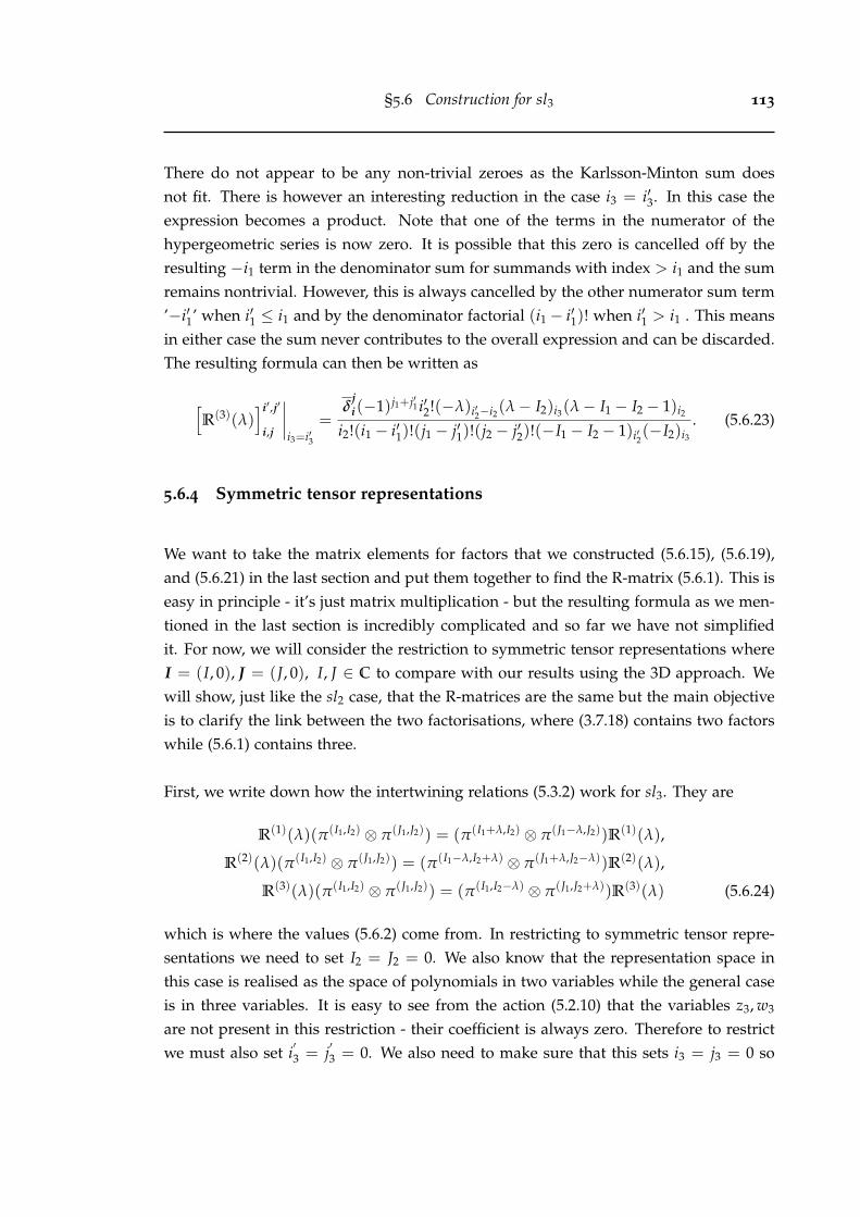
§5.6 Construction for sl3 113
There do not appear to be any non-trivial zeroes as the Karlsson-Minton sum doesnot fit. There is however an interesting reduction in the case i3 = i′3. In this case theexpression becomes a product. Note that one of the terms in the numerator of thehypergeometric series is now zero. It is possible that this zero is cancelled off by theresulting −i1 term in the denominator sum for summands with index > i1 and the sumremains nontrivial. However, this is always cancelled by the other numerator sum term’−i′1’ when i′1 ≤ i1 and by the denominator factorial (i1 − i′1)! when i′1 > i1 . This meansin either case the sum never contributes to the overall expression and can be discarded.The resulting formula can then be written as
[R(3)(λ)
]i′,j′
i,j
∣∣∣∣i3=i′3
=δ
ji(−1)j1+j′1 i′2!(−λ)i′2−i2(λ− I2)i3(λ− I1 − I2 − 1)i2
i2!(i1 − i′1)!(j1 − j′1)!(j2 − j′2)!(−I1 − I2 − 1)i′2(−I2)i3
. (5.6.23)
5.6.4 Symmetric tensor representations
We want to take the matrix elements for factors that we constructed (5.6.15), (5.6.19),and (5.6.21) in the last section and put them together to find the R-matrix (5.6.1). This iseasy in principle - it’s just matrix multiplication - but the resulting formula as we men-tioned in the last section is incredibly complicated and so far we have not simplifiedit. For now, we will consider the restriction to symmetric tensor representations whereI = (I, 0), J = (J, 0), I, J ∈ C to compare with our results using the 3D approach. Wewill show, just like the sl2 case, that the R-matrices are the same but the main objectiveis to clarify the link between the two factorisations, where (3.7.18) contains two factorswhile (5.6.1) contains three.
First, we write down how the intertwining relations (5.3.2) work for sl3. They are
R(1)(λ)(π(I1,I2) ⊗ π(J1,J2)) = (π(I1+λ,I2) ⊗ π(J1−λ,J2))R(1)(λ),
R(2)(λ)(π(I1,I2) ⊗ π(J1,J2)) = (π(I1−λ,I2+λ) ⊗ π(J1+λ,J2−λ))R(2)(λ),
R(3)(λ)(π(I1,I2) ⊗ π(J1,J2)) = (π(I1,I2−λ) ⊗ π(J1,J2+λ))R(3)(λ) (5.6.24)
which is where the values (5.6.2) come from. In restricting to symmetric tensor repre-sentations we need to set I2 = J2 = 0. We also know that the representation space inthis case is realised as the space of polynomials in two variables while the general caseis in three variables. It is easy to see from the action (5.2.10) that the variables z3, w3
are not present in this restriction - their coefficient is always zero. Therefore to restrictwe must also set i
′3 = j
′3 = 0. We also need to make sure that this sets i3 = j3 = 0 so

114 R-matrix factorisation by Q-operators
that our operator does not map out of the subspace C[z1, z2]. We will soon show that isindeed the case. In this restriction the R-matrix (5.6.1) simplifies considerably, and theelements can be written as
[RI,J(λ)]i′,j′
i,j = P ∑s,lr,t
[R1(λ +
2J − 2I3
∣∣∣∣− λ +2I + J
3, 0; λ +
2J + I3
, 0)]s1,s2,s3,l1,l2,l3
i1,i2,i3,j1,j2,j3
×[
R2(λ +I − J
3
∣∣∣∣ I,−λ +J − I
3; J, λ +
I − J3
)
]r1,r2,r3,t1,t2,t3
s1,s2,s3,l1,l2,l3
×[
R3(λ +I − J
3
∣∣∣∣ I, 0; J, 0)]i′1,i′2,0,j′1,j′2,0
r1,r2,r3,t1,t2,t3
(5.6.25)
It appears that there are twelve summations but actually this can be reduced quitedrastically. In fact, we claim that
r3 = s3 = l3 = i3 = j3 = 0.
This is justified by our consideration of the reductions of each factor R(i) in the previoussection where we found regimes where the elements of each factor can be zero or asimple product. Let us expain, starting from the upper indices and working downward.The summation index r3 must be zero because i′3 = 0 and (5.6.22) implies that r3 = 0 elsethe expression is trivial. l3 = 0 by examining R(2) (5.6.19) is trivially zero when λ = J2
and l3 > 0. In (5.6.25) this equality holds. j3 = 0 in R(1) because J2 = 0, l3 = 0 and thereduction (5.6.17). If s3 = 0, then clearly by the delta function in (5.6.15) we must havei3 = 0 also. The justification that s3 = 0 is more complicated. While s3 > r3 = 0 in R(2)
(5.6.19) is in general non-zero, R(2)R(3) in (5.6.25) it seems it is always zero. This wediscovered by evaluating the resulting expression for this range of values, although itseems to be a highly non-trivial zero that results from some complicated interplay of aquadruple summation. We expect it to be true because of the way R(2)R(3) in (5.6.25)intertwines the representation, i.e.
R(2)R(3)(λ)(π(I,0) ⊗ π(J,0)) = (π(−λ+ 2I+J3 ,0) ⊗ π(λ+ 2J+I
3 ,0))R(2)R(3)(λ)
preserving the (non-)zero nature of each component. Therefore R(2)R(3) should pre-serve the subspace C[z1, z2]. We also remark that R(1) in (5.6.25) preserves this sub-space, as justified in the last paragraph, and indeed by (5.6.24) it preserves the weights.So we set s3 = 0. Another interesting feature of (5.6.25) is that t3 is a non-trivial sum-mation and so it can be said that although the operator R(2)R(3) together preserves thesubspace the individual factors map out of it even when I2 = J2 = 0. Indeed, theseweight arguments for R(2) in (5.6.25) are non-zero and actually depend on I, J.

§5.6 Construction for sl3 115
Let us now consider the implications of our discussion so far for the expressions forR(i) we use in constructing the R-matrix (5.6.25). For R(1) we use the product formula(5.6.17). For R(2) we use the product formula (5.6.20) and for R(3) we use the productformula (5.6.23). All the regimes where these reductions hold are satisfied. Followingfrom (5.6.18) therefore we have already identified one of our factors (3.7.18) in (5.6.25)and now we will prove that the other factor comes from R(2)R(3) in a non-trivial way.We will do this by showing the expression for its elements are given by the same prod-uct function as Mr.
Putting together R(2)R(3) we see that there are five summations r3, r2, t1, t2, t3. Thereare also four kronecker delta functions which allow us to remove two of these vari-ables. We choose to eliminate t1, t2 by making the substitution t1 := i′1 + j′1 + t3 −r1, t2 := i′2 + j′2 − r2 − t3. In what follows, we rename the remaining summation indicess := r1, t := r2, l := t3, and also s1 := i1, s2 := i2, l1 := j1, l2 := j2 because these are nowlower indices for the purposes of our computation. After all, we find the expression forthe matrix elements is given by
[R(2)R(3)(λ)
]i′,j′
i,j= δi+j,i′+j′
(−1)i1+i2+i′1+i′2(λ− 2I+J3 )i1
i1!i2!(i′2 − i2)!(−1− I)i′2(λ + 1 + I−J
3 )i1
(5.6.26)
× ∑s,l,t=0
(−1)ss!l!(−λ + J−I3 − i1)s(−i′2)l
(s− l − i1, s− i′1, l + i′1 − s)!(−I)s3F2
(l − i′2; λ− 2I+J
3 − 1 −i2λ + I−J
3 + 1− i′2 1 + l − i2
∣∣∣∣∣ 1
).
The formula is a triple summation in variables 0 ≤ l ≤ i′2, i′1 ≤ s ≤ i′1 + l and theterminating 3F2 hypergeometric series (whose summation variables we call ‘t’) whichterminates after i′2 − l terms. These bounds ensure that the variable substitution madein the last paragraph do not sum up negative values of summation indices. For theKronecker delta function we have used the notation (3.3.12). Note that the expression istrivially zero unless i′2 ≥ i2 because of the factorial term outside the sum which can benegative. The first step is to transform this identity with the second Thomae theorem(A.2.5) (with the given ordering) to obtain
[R(2)R(3)(λ)
]i′,j′
i,j= δi+j,i′+j′
(−1)i1+i2+i′1(λ− 2I+J3 )i1
i1!i2!(i′2 − i2)!(−1− I)i′2(λ + 1 + I−J
3 )i1
(5.6.27)
× ∑s,l,t=0
(−1)l+ss!l!(−λ + J−I3 − i1)s(−i′2)l
(s− l − i1)!(s− i′1)!(l + i′1 − s)!(−I)s3F2
(l − i′2; −i2 2 + I − i′2
−i′2 λ + I−J3 + 1− i′2
∣∣∣∣∣ 1
),

116 R-matrix factorisation by Q-operators
as an intermediate step. Making this transform affects the expression for the othersummations so that they can be transformed into a product. In particular, we rewrite(5.6.27) by bringing the summation in ‘l’ forward and identifying it as a 3F2 hypergeo-metric series. That is
[R(2)R(3)(λ)
]i′,j′
i,j= δi+j,i′+j′
(−1)i2+i′1 i′2!(λ− 2I+J3 )i1(−λ + J−I
3 )i′2i1!i2!(i′2 − i2)!(i′1 − i1)!(−1− I)i′2
(5.6.28)
× ∑s,l,t=0
(−1)ss!(−i2, 2 + I − i′2)t
t!(s− i1, s− i′1)!(−I)s(λ + I−J3 − i′2 + 1)t
3F2
(i1 − s; t− i′2 1
1 + i′1 − s −λ + J−I3
∣∣∣∣∣ 1
).
This series can be summed to a product using the identity (A.2.12) but we must dothis carefully. First let us note that we can assume i′1 ≥ i1 and i′2 ≥ i2 because theexpression is trivially zero otherwise because of the denominator factorials outside thesum. Secondly, it is easy to see that the sum in t ≤ i2 and s ≥ i′1, therefore we canassume that i1 − s ≤ 0, t− i′2 ≤ 0 and s− i1 ≥ s− i′1. Therefore we can safely apply(A.2.12) with n1 = s− i1, n2 = s− i′1 and a = t− i′2 to obtain
[R(2)R(3)(λ)
]i′,j′
i,j= δi+j,i′+j′
(−1)i2+i′1 i′2!(−λ + J−I3 )i′1+i′2−i1(λ−
2I+J3 )i1
i1!i2!(i′2 − i2)!(i′1 − i1)!(i′1 + i′2)!(−1− I)i′2(−I)i′1+i′2
(5.6.29)
× ∑s,t=0
(−i2,−i′1 − i′2, 2 + I − i′2, I + 1− i′1 − i′2)t
t!(λ + I−J3 + 1 + i1 − i′1 − i′2)t
3F2
(t− i′1 − i′2; 1 1
1− i′1 −I
∣∣∣∣∣ 1
),
where we have written the resulting double summation by bringing forward the seriesin ‘s’ and identifying it as a 3F2 hypergeometric series. It is easy to see that t ≤ i2 andhence i1 + i′2 − t ≥ i′1 ≥ 0. Therefore it can be summed with identity (A.2.12) and doingso we obtain
[R(2)R(3)(λ)
]i′,j′
i,j= δi+j,i′+j′
(−1)i2 i′1!i′2!(−λ + J−I3 )i′1+i′2−i1(λ−
2I+J3 )i1
i1!i2!(i′2 − i2)!(i′1 − i1)!(−I)i′1+i′2
(5.6.30)
× 2F1
(−i2 I + 1− i′1 − i′2
λ + I−J3 + 1 + i1 − i′1 − i′2
∣∣∣∣∣ 1
).
The 2F1 is easily transformed using Gauss’ sum (A.2.2). Finally we find matrix elementsare given by the product
[R(2)R(3)(λ)
]i′,j′
i,j= δi+j,i′+j′
i′1!i′2!(λ− 2I+J3 )i1+i2(−λ + J−I
3 )i′1+i′2−i1−i2
i1!i2!(i′2 − i2)!(i′1 − i1)!(−I)i′1+i′2
. (5.6.31)

§5.6 Construction for sl3 117
Immediately we see that this function is essentially the same as R(1)(λ) in the reduction(5.6.17) but with i(
′) and j(′) insides swapped. Specifically, when i(
′)3 , j(
′)3 = 0
[R(1)(λ +
I − J3|J, 0; I, 0)
]j′,i′
j,i=[R(2)R(3)(λ|I, J)
]i′,j′
i,j. (5.6.32)
Now we can make the connection with our factorisation in the rational limit (3.7.18).Since we already identified R(1) with Nr in (5.6.18) we compare R(2)R(3) to Mr and seethat
R(2)R(3)(µ|µ +I + J
2, µ + 2J − I) = PMr, (5.6.33)
so they are the same up to some change of variables for I, J. We remind the reader thatthough we have written the function with a dependence on three variables, there areonly two independent ones. That is the substitution made in (5.6.33) is not unique.
Now we can evaluate (5.6.25) using (5.6.17) and (5.6.31). We first need to make therequired substitutions in R(1)(λ|I, J) for the variables λ, I, J. It is easy to see from(5.6.25) that the expression will have four summations in variables s11, s12, l11, l12 butalso four Kronecker delta functions, which allow us to remove two of these summa-tions. We eliminate variables l11, l12 by making the subsitution l11 := i′1 + j′1− s11, l12 :=i′2 + j′2 − s12 to get a double sum formula for the elements of the sl3 R-matrix acting onthe tensor product of Verma modules VI ⊗ VJ . As expected, this double sum formulais essentially the same as (3.7.4) in the case n = 3. In fact, they are identical up to asymmetry and change of variables, the explicit relationship is
[R(3),r
J,I (λ)]j′,i′
j,i=(
PR(1)R(2)R(3))(λ +
I − J6
), (5.6.34)
where the argument on the right hand side is the overall dependence of the expressionon the spectral parameter, not the individual factors. The left hand side has the indicesand weight parameters swapped but we established in symmetry (3.7.21a) that thisdoes not affect the function. Therefore they are equal. This swapping of indices is thesame as the sl2 case where to get an identical expression (5.5.16) we had to reverse theordering of the factors. This is the same for the sl3 case where we can just reverse theordering of R(1) and R(2)R(3), where we find
[R(3),r
I,J (λ)]i′,j′
i,j=(
PR(2)R(3)R(1))(λ +
I − J6
). (5.6.35)
118 R-matrix factorisation by Q-operators
Some care needs to be taken in computing this; the operators R(2)R(3) and R(1) take dif-ferent arguments for weight parameters I, J in (5.6.35) compared to (5.6.34) and (5.6.25)because of their new relative positions in the product and their nature as intertwinersof the representation.
5.6.5 Discussion
For the sl3 case we have established the relation between our factorisation (3.7.18) andthat of this chapter and shown that they are the same R-matrix. It is interesting to com-pare with what happens in the sl2 case, whose R(1) factor is clearly contained withinthe same factor for sl3 but the second factor is actually contained in R(2)R(3). It is inter-esting that although this product preserves the subspace C[z1, z2] there is a contribution(the variable t3) to its overall form coming from outside the space.
We expect that our sln R-matrix (3.7.4) can be constructed by considering the factori-sation (5.1.8) but this could be quite difficult because we have to construct each factorin its entire form for all highest weight representations and then restrict afterwards.From our experience of considering sl4, the complexity of these objects grow incrediblyfast with n and it appears hopeless unless a pattern for its growth can be found. Forexample, the complexity of the formula (3.3.18) using the 3D approach grows in a sim-ple pattern with n and the Lagrange interpolation formula (3.3.20) can be used to sumthem up all at the same time. However, even with each factor in its simplest form therestriction to symmetric tensor representation is quite a large computation. In derivingthe reductions of the last section and then transforming (5.6.26) to (5.6.31) we see it isa non-trivial task using many powerful identities. We are confident then, that for thisclass of representations the 3D model approach is the most efficient at constructing theR-matrix.
Our primary interest for considering the restriction was to see how the n factors of(5.1.8) go to only two (essentially equal) factors in (3.7.18). We have shown how thisoccurs for n = 2, 3 and conjecture for general n that
Nr ∼ R(1),
Mr ∼ PR(2)R(3) . . . R(n).
§5.6 Construction for sl3 119
This identification is based on the way each factor intertwines the representations, thatis
R(k)(λ)(πI ⊗ π J) = (πI+λk ⊗ π J−λk)R(k)(λ),
I ± λk = (I1, . . . ,Ik−1 ∓ λ, Ik ± λ, . . . , In−1)
and hence for sln
R(1)(λ)(π(I1,0,...,0) ⊗ π(J1,0,...,0)) = (π(I1+λ,0,...,0) ⊗ π(J1−λ,0,...,0))R(1)(λ),
R(2)R(3) . . . R(n)(λ)(π(I1,0,...,0) ⊗ π(J1,0,...,0)) =
(π(I1−λ,0,...,0) ⊗ π(J1+λ,0,...,0))R(2)R(3) . . . R(n)(λ).
So these operators preserve the (non-)zero nature of each weight component and shouldpreserve the symmetric tensor representation subspace C[z21, . . . , zn1].

120 R-matrix factorisation by Q-operators
Chapter 6
L-operator factorisation
In this chapter we will study a factorisation of the sl2 L-operator and generalise itto Uq(sl2). The construction of this factorisation gives another way of constructing aformula for the elements of the rational sl2 R-matrix, which is different again to theformulae obtained by the methods in other chapters. The formula is a finite dou-ble sum expression but can to summed up to the 4F3 (3.8.5) first obtained using the3-dimensional projection approach. Using the quantum deformation (3.8.3) we can re-verse the arguments to obtain the analogous double sum for the Uq(sl2) R-matrix. Uponinspection of this formula, we see it can be split into factors of the same form as therational case. The factorisation holds for the R-matrix acting on CI+1⊗VJ and thereforeis a factorisation of the higher spin Uq(sl2) L-operator.
The factorisation in the rational case is related to the construction in chapter 5 butis different. The factorisation in that chapter is for the R-matrix acting on Verma mod-ules and although the action can be restricted to a finite dimensional subspace whenthe weights are integral, the individual factors cannot as they map out of the subspace- it is a ‘rectangular’ factorisation. In contrast, the factorisation we study in this chap-ter holds for finite dimensional representations and the factors can be written down asfinite square matrices. In the case of the L-operator we get a square factorisation withoperator entries.
The overview the method, developed in [11; 12], we begin by writing down the sl2R-matrix in the factorised differential operator form (5.1.7) and (5.1.8) first introducedin [13]:
RI J(µ) = P12Γ(z21∂2 − I)
Γ(z21 − µ− I+J2 )
Γ(z12∂1 + µ− I+J2 )
Γ(z12∂1 − I). (6.0.1)
121
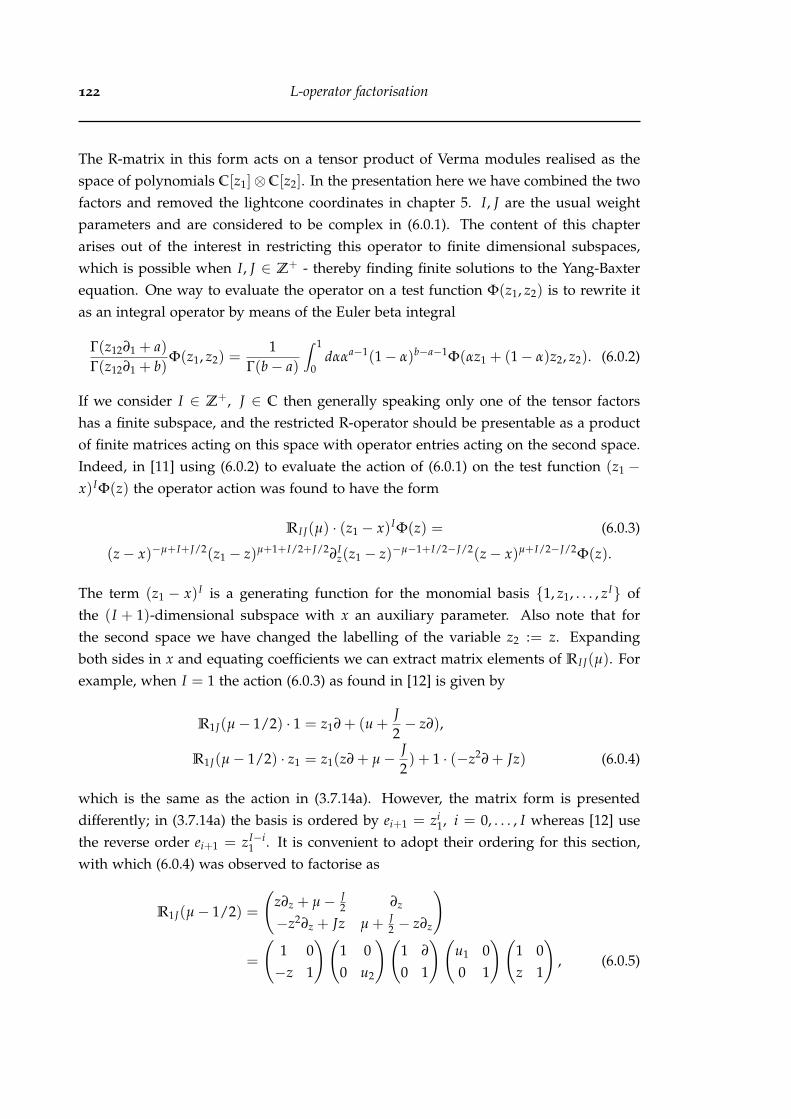
122 L-operator factorisation
The R-matrix in this form acts on a tensor product of Verma modules realised as thespace of polynomials C[z1]⊗C[z2]. In the presentation here we have combined the twofactors and removed the lightcone coordinates in chapter 5. I, J are the usual weightparameters and are considered to be complex in (6.0.1). The content of this chapterarises out of the interest in restricting this operator to finite dimensional subspaces,which is possible when I, J ∈ Z+ - thereby finding finite solutions to the Yang-Baxterequation. One way to evaluate the operator on a test function Φ(z1, z2) is to rewrite itas an integral operator by means of the Euler beta integral
Γ(z12∂1 + a)Γ(z12∂1 + b)
Φ(z1, z2) =1
Γ(b− a)
∫ 1
0dααa−1(1− α)b−a−1Φ(αz1 + (1− α)z2, z2). (6.0.2)
If we consider I ∈ Z+, J ∈ C then generally speaking only one of the tensor factorshas a finite subspace, and the restricted R-operator should be presentable as a productof finite matrices acting on this space with operator entries acting on the second space.Indeed, in [11] using (6.0.2) to evaluate the action of (6.0.1) on the test function (z1 −x)IΦ(z) the operator action was found to have the form
RI J(µ) · (z1 − x)IΦ(z) = (6.0.3)
(z− x)−µ+I+J/2(z1 − z)µ+1+I/2+J/2∂Iz(z1 − z)−µ−1+I/2−J/2(z− x)µ+I/2−J/2Φ(z).
The term (z1 − x)I is a generating function for the monomial basis 1, z1, . . . , zI ofthe (I + 1)-dimensional subspace with x an auxiliary parameter. Also note that forthe second space we have changed the labelling of the variable z2 := z. Expandingboth sides in x and equating coefficients we can extract matrix elements of RI J(µ). Forexample, when I = 1 the action (6.0.3) as found in [12] is given by
R1J(µ− 1/2) · 1 = z1∂ + (u +J2− z∂),
R1J(µ− 1/2) · z1 = z1(z∂ + µ− J2) + 1 · (−z2∂ + Jz) (6.0.4)
which is the same as the action in (3.7.14a). However, the matrix form is presenteddifferently; in (3.7.14a) the basis is ordered by ei+1 = zi
1, i = 0, . . . , I whereas [12] usethe reverse order ei+1 = zI−i
1 . It is convenient to adopt their ordering for this section,with which (6.0.4) was observed to factorise as
R1J(µ− 1/2) =
(z∂z + µ− J
2 ∂z
−z2∂z + Jz µ + J2 − z∂z
)
=
(1 0−z 1
)(1 00 u2
)(1 ∂
0 1
)(u1 00 1
)(1 0z 1
), (6.0.5)

§6.1 Factorization formula for the rational R-matrix 123
where u1 = µ− J/2− 1 and u2 = µ + J/2. It turns out that a factorisation of this formexists for all I ∈ Z+, J ∈ C. That is,
RI J(µ− I/2) = Z−1U+(u2)DU−(u1)Z. (6.0.6)
The factors Z, U±(u) and D are (I + 1)-dimensional square matrices in general. It canbe shown they have the operator form
Z = exp (z∂z1) , D = Cexp(∂z∂z1)C, U−(u) =Γ(z1∂z1 + u + 1− I)
Γ(u + 1− I),
U+(u) = CU−(u)C, C · zi1 = zI−i
1 (6.0.7)
acting on C[z1]⊗C[z]. By considering this operator action on (z1 − x)IΦ(z) Chicherin-Derkachov [12] derive the following formula:
[RI J(µ−
I2)
]·[(z1 − x)IΦ(z)
]=
I
∑k=0
I!k!(I − k)!
Γ(u1 + 1− I + k)Γ(u1 + 1− I)
×I−k
∑p=0
(I − k)!p!(I − k− p)!
Γ(u2 + 1− k− p)Γ(u2 + 1− I)
(z1 − z)k+p∂pz
[(z− x)I−kΦ(z)
]. (6.0.8)
It was proven in [12] that this action is the same as (6.0.3) thereby proving the factorisa-tion (6.0.6-6.0.7). It is from (6.0.8) we begin our construction of a formula for the matrixelements of RI J(µ) and show that it is the same formula as (3.8.5) and hence showingthis method is equivalent to all of the others.
6.1 Factorization formula for the rational R-matrix
Let us substitute into (6.0.8) Φ(z) = zj′ and expand in powers of x. As an intermediatestep we have
I
∑i′=0
I!(−x)I−i′
(I − i′)!i′!
[RI J(u− I/2) · zi′
1 zj′]=
I
∑k=0
(−I)k(−1)k
(1)k(u1 − I + 1)k
×I−k
∑p=0
(−1)p(k− I)p
(1)p
Γ(u2 + 1− k− p)Γ(u2 + 1− I)
k+p
∑i=0
(−k− p)i(−1)k+p
(1)izi
1zk+p−i
×I−k
∑s=0
(I − k)!(I − k− s + j′)!(−1)s
(I − k− s)!s!(I − k− s + j′ − p)!zI−k−s+j′−pxs, (6.1.1)

124 L-operator factorisation
where all we have done is expand out binomial terms with the binomial theorem andapply the differential operator action on the basis. In equating powers of x we sets = I − i′. We also fix i′ on the left hand side and collect powers of z, z1. After someeasy simplifications of Gamma functions and pochammer symbols using (A.1.1) we getthe following result for the action of the operator RI J(µ− I
2 ):
RI J(µ−I2) · zi′
1 zj′ =I
∑i=0
zi1zi′+j′−i
[RI J(µ−
I2)
]i′,j′
i,i′+j′−i, (6.1.2)
where [RI J(µ−
I2)
]i′,j′
i,i′+j′−i=
i′!I!i!
I
∑k=0
I−k
∑p=0
(−I, µ− I − J/2)k(I − k)!(k− I)p
k!p!
×(i′ − k + 1)j′(µ− I + J/2 + 1)I−k−p(−k− p)i
(i′ + j′ − k− p)!. (6.1.3)
The summation of i seems to imply that index i′ + j′ − i can be negative. Indeed it can,however, the function is always zero in this case. This is a consequence of the numeratorpochammer (−k − p)i eliminating summands where k + p < i and the denominatorterm (i′ + j′ − k− p)! eliminating summands where i′ + j′ < k + p. To compare (6.1.3)with (3.8.5) we first reverse the spectral parameter shift and divide by the factor
C(µ; I, J) = (µ +J − I
2+ 1)I , (6.1.4)
in effect defining the function RrI J(µ) for the matrix elements by
[RI J(µ)]i′,j′
i,j = C(µ; I, J)[Rr
I J(µ)]i′,j′
i,j . (6.1.5)
Making a few further simplifications we finally get the formula
[Rr
I J(µ)]i′,j′
i,j = δi+j,i′+j′i′
∑k=0
I−k
∑p=0
(−1)k (−i′, µ− I+J2 )k(k− I,−i− j + k)p(−k− p)i
i! k! p!(−µ− I+J2 )k+p
. (6.1.6)
Let us notice that the operator RrI J(µ) is normalised similar to (3.3.29), i.e.
[Rr
I J(µ)]0,0
0,0 = 1. (6.1.7)
It is easy to see that the operator Rr12(µ) can be now defined for any I ∈ C. Initially
the action of the operator RI J(µ) was defined only for I ∈ Z+. However, after extract-ing the factor C(µ; I, J) the resulting expression can be transformed to the form (6.1.6)
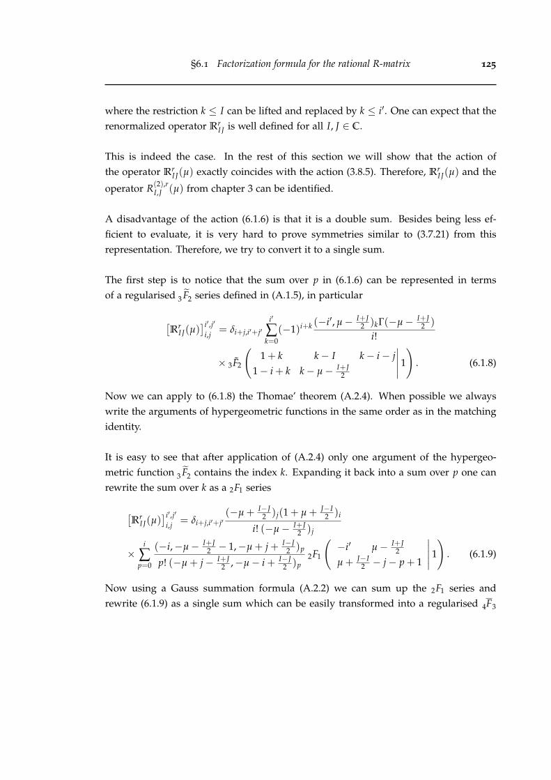
§6.1 Factorization formula for the rational R-matrix 125
where the restriction k ≤ I can be lifted and replaced by k ≤ i′. One can expect that therenormalized operator Rr
I J is well defined for all I, J ∈ C.
This is indeed the case. In the rest of this section we will show that the action ofthe operator Rr
I J(µ) exactly coincides with the action (3.8.5). Therefore, RrI J(µ) and the
operator R(2),rI,J (µ) from chapter 3 can be identified.
A disadvantage of the action (6.1.6) is that it is a double sum. Besides being less ef-ficient to evaluate, it is very hard to prove symmetries similar to (3.7.21) from thisrepresentation. Therefore, we try to convert it to a single sum.
The first step is to notice that the sum over p in (6.1.6) can be represented in termsof a regularised F3 2 series defined in (A.1.5), in particular
[Rr
I J(µ)]i′,j′
i,j = δi+j,i′+j′i′
∑k=0
(−1)i+k (−i′, µ− I+J2 )kΓ(−µ− I+J
2 )
i!
× 3F2
(1 + k k− I k− i− j
1− i + k k− µ− I+J2
∣∣∣∣∣ 1
). (6.1.8)
Now we can apply to (6.1.8) the Thomae’ theorem (A.2.4). When possible we alwayswrite the arguments of hypergeometric functions in the same order as in the matchingidentity.
It is easy to see that after application of (A.2.4) only one argument of the hypergeo-metric function F3 2 contains the index k. Expanding it back into a sum over p one canrewrite the sum over k as a 2F1 series
[Rr
I J(µ)]i′,j′
i,j = δi+j,i′+j′(−µ + I−J
2 )j(1 + µ + J−I2 )i
i! (−µ− I+J2 )j
×i
∑p=0
(−i,−µ− I+J2 − 1,−µ + j + I−J
2 )p
p! (−µ + j− I+J2 ,−µ− i + I−J
2 )p2F1
(−i′ µ− I+J
2
µ + J−I2 − j− p + 1
∣∣∣∣∣ 1
). (6.1.9)
Now using a Gauss summation formula (A.2.2) we can sum up the 2F1 series andrewrite (6.1.9) as a single sum which can be easily transformed into a regularised F4 3

126 L-operator factorisation
series. We obtain
[Rr
I J(µ)]i′,j′
i,j = δi+j,i′+j′(−1)i
i!(−J)j(−µ + I−J
2 )j−i′
(−J)j′(−µ− I+J2 )i+j
× 4F3
(−i; j− J −µ− I+J
2 − 1 −µ + I−J2 + j− i′
−µ− I+J2 + j −µ + I−J
2 − i j− i′ − J
∣∣∣∣∣ 1
).
(6.1.10)
As the last step we apply the identity (A.2.13) to (6.1.10) and obtain exactly the expres-sion on the right-hand side of (3.8.5). Let us note that all transformations between (3.8.5)and (6.1.6) are valid for any complex I, J. Therefore it justifies our previous statementthat the renormalized operator Rr
12 is defined by its action (6.1.6) for I, J ∈ C.
6.2 The trigonometric R-matrix
In this section we construct a trigonometric factorization of the general R-matrix actingin VI ⊗ V+
J , I ∈ Z+, J ∈ C similar to [12]. However, there is a noticeable differencebetween our result and their approach. In [12] the authors considered a more generalcase of the so called modular double. As well known in the standard q-deformed casethe R-matrix can not be calculated uniquely from the L-operator intertwining relationsdue to the presence of a large center in the Uq(sl2) algebra on the space of continuousfunctions. This problem can be naturally solved using the modular double of the quan-tum group [68].
In principle one can derive a factorization of the standard R-matrix restricting a con-struction of [12] to a “half” of the representation of the modular double. However, weprefer to reverse the arguments of the previous section and first obtain the q-analogof the formula (6.0.8) starting from the hypergeometric representation of the XXZ R-matrix (3.8.3). Then we show how this q-analog allows a natural factorization.
First we start from (3.8.3) with I, J ∈ C and apply the identity (B.2.14) with n = iand
a = λ2q2−I+J , b = q−2i′ , c = λ−2qJ−I ,
d = q2(1−i−j+J), e = q−2I , f = q2(1+j−i′)
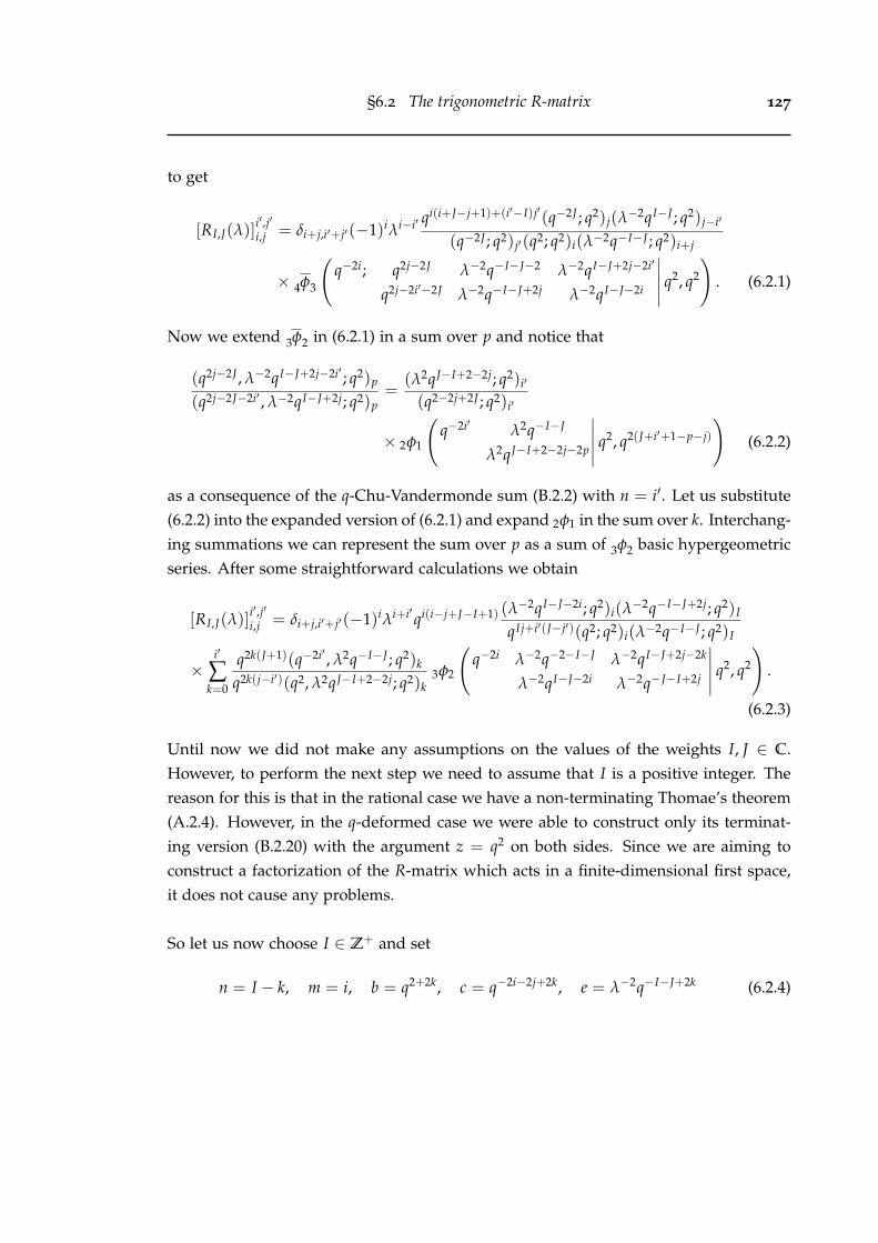
§6.2 The trigonometric R-matrix 127
to get
[RI,J(λ)]i′,j′
i,j = δi+j,i′+j′(−1)iλi−i′ qi(i+J−j+1)+(i′−I)j′(q−2J ; q2)j(λ
−2qI−J ; q2)j−i′
(q−2J ; q2)j′(q2; q2)i(λ−2q−I−J ; q2)i+j
× φ4 3
(q−2i; q2j−2J λ−2q−I−J−2 λ−2qI−J+2j−2i′
q2j−2i′−2J λ−2q−I−J+2j λ−2qI−J−2i
∣∣∣∣∣ q2, q2
). (6.2.1)
Now we extend φ3 2 in (6.2.1) in a sum over p and notice that
(q2j−2J , λ−2qI−J+2j−2i′ ; q2)p
(q2j−2J−2i′ , λ−2qI−J+2j; q2)p=
(λ2qJ−I+2−2j; q2)i′
(q2−2j+2J ; q2)i′
× 2φ1
(q−2i′ λ2q−I−J
λ2qJ−I+2−2j−2p
∣∣∣∣∣ q2, q2(J+i′+1−p−j)
)(6.2.2)
as a consequence of the q-Chu-Vandermonde sum (B.2.2) with n = i′. Let us substitute(6.2.2) into the expanded version of (6.2.1) and expand 2φ1 in the sum over k. Interchang-ing summations we can represent the sum over p as a sum of φ3 2 basic hypergeometricseries. After some straightforward calculations we obtain
[RI,J(λ)]i′,j′
i,j = δi+j,i′+j′(−1)iλi+i′qi(i−j+J−I+1) (λ−2qI−J−2i; q2)i(λ
−2q−I−J+2j; q2)I
qI j+i′(J−j′)(q2; q2)i(λ−2q−I−J ; q2)I
×i′
∑k=0
q2k(J+1)(q−2i′ , λ2q−I−J ; q2)k
q2k(j−i′)(q2, λ2qJ−I+2−2j; q2)k3φ2
(q−2i λ−2q−2−I−J λ−2qI−J+2j−2k
λ−2qI−J−2i λ−2q−J−I+2j
∣∣∣∣∣ q2, q2
).
(6.2.3)
Until now we did not make any assumptions on the values of the weights I, J ∈ C.However, to perform the next step we need to assume that I is a positive integer. Thereason for this is that in the rational case we have a non-terminating Thomae’s theorem(A.2.4). However, in the q-deformed case we were able to construct only its terminat-ing version (B.2.20) with the argument z = q2 on both sides. Since we are aiming toconstruct a factorization of the R-matrix which acts in a finite-dimensional first space,it does not cause any problems.
So let us now choose I ∈ Z+ and set
n = I − k, m = i, b = q2+2k, c = q−2i−2j+2k, e = λ−2q−I−J+2k (6.2.4)

128 L-operator factorisation
in the regularized identity (B.2.20). After straightforward transformation we get thefollowing answer:
[RI,J(λ)]i′,j′
i,j = δi+j,i′+j′(−1)iλi′−i qi(i−j−1)+I j+i′(j′−J)
(q2; q2)i
×∑k,p
(−1)k
λ2k
(q−2i′ , λ2q−I−J ; q2)k(q2k−2i′−2j′ ; q2)p(q2, q−2I ; q2)k+p
(q2, q−2I ; q2)k(q2; q2)p(q2; q2)k+p−i(λ−2q−I−J ; q2)k+pqk2+k(J−I−2j′+1)+2p.
(6.2.5)
The summation variables k and p in (6.2.5) are restricted as
0 ≤ k ≤ i′, 0 ≤ p ≤ (i′ − k) + j′, i ≤ k + p. (6.2.6)
The formula (6.2.5) gives a q-deformation of (6.1.6) as can be easily seen by taking thelimit q→ 1.
6.3 A trigonometric factorization
A factorised form of the R-matrix acting on the tensor product of an arbitrary finitedimensional and arbitrary infinite dimensional representations of the modular doublewas derived in (44) of [12]. More explicitly, the authors of [12] considered only spe-cial restricted representations corresponding to a “half” of the modular double. It isnatural to expect that the R-matrix (44) from [12] should be related to our higher-spinR-matrix (6.2.5). In this section we shall derive this type of factorization directly from(6.2.5). As we shall see there is a slight difference between our results and results of [12].
First, let us remind that the operator RI,J(λ) is realized on the space of polynomialsin variables z1 and z by its action on the basis
RI,J(λ) · zi′1 zj′ = ∑
i,j[RI,J(λ)]
i′,j′
i,j zi1zj. (6.3.1)
When I is a positive integer we can represent RI,J(λ) by the (I + 1)× (I + 1)-dimensionalmatrix with operator entries acting in the space C[z]. It is obvious that this matrix co-incides with a particular realization of the (I + 1)-dimensional L-operator acting in theVerma module VJ .
To write down the explicit formulas for the L-operator we make two simple similar-
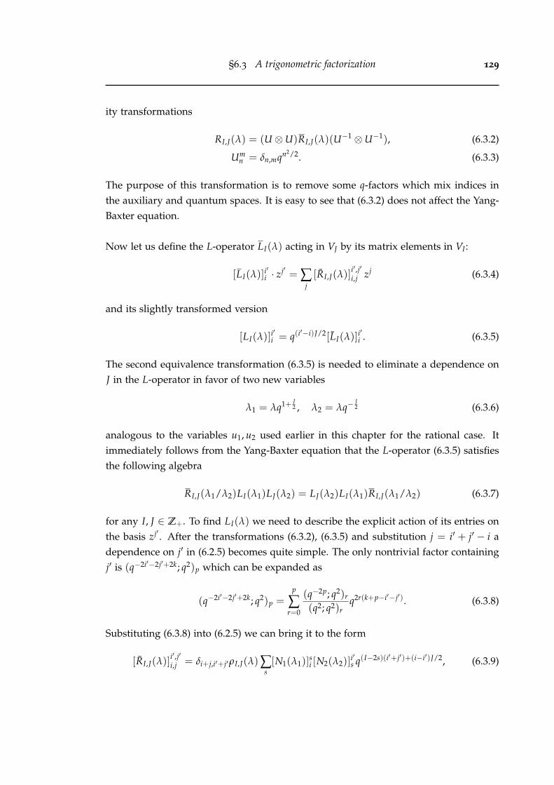
§6.3 A trigonometric factorization 129
ity transformations
RI,J(λ) = (U ⊗U)RI,J(λ)(U−1 ⊗U−1), (6.3.2)
Umn = δn,mqn2/2. (6.3.3)
The purpose of this transformation is to remove some q-factors which mix indices inthe auxiliary and quantum spaces. It is easy to see that (6.3.2) does not affect the Yang-Baxter equation.
Now let us define the L-operator LI(λ) acting in VJ by its matrix elements in VI :
[LI(λ)]i′i · zj′ = ∑
j[RI,J(λ)]
i′,j′
i,j zj (6.3.4)
and its slightly transformed version
[LI(λ)]i′i = q(i
′−i)J/2[LI(λ)]i′i . (6.3.5)
The second equivalence transformation (6.3.5) is needed to eliminate a dependence onJ in the L-operator in favor of two new variables
λ1 = λq1+ J2 , λ2 = λq−
J2 (6.3.6)
analogous to the variables u1, u2 used earlier in this chapter for the rational case. Itimmediately follows from the Yang-Baxter equation that the L-operator (6.3.5) satisfiesthe following algebra
RI,J(λ1/λ2)LI(λ1)LJ(λ2) = LJ(λ2)LI(λ1)RI,J(λ1/λ2) (6.3.7)
for any I, J ∈ Z+. To find LI(λ) we need to describe the explicit action of its entries onthe basis zj′ . After the transformations (6.3.2), (6.3.5) and substitution j = i′ + j′ − i adependence on j′ in (6.2.5) becomes quite simple. The only nontrivial factor containingj′ is (q−2i′−2j′+2k; q2)p which can be expanded as
(q−2i′−2j′+2k; q2)p =p
∑r=0
(q−2p; q2)r
(q2; q2)rq2r(k+p−i′−j′). (6.3.8)
Substituting (6.3.8) into (6.2.5) we can bring it to the form
[RI,J(λ)]i′,j′
i,j = δi+j,i′+j′ρI,J(λ)∑s[N1(λ1)]
si [N2(λ2)]
i′s q(I−2s)(i′+j′)+(i−i′)J/2, (6.3.9)

130 L-operator factorisation
where N1,2(λ1,2) are two numerical (I + 1)× (I + 1)-dimensional matrices, ρI,J(λ) is aconstant multiplier and λ1,2 are defined in (6.3.6).
The explicit form of matrices N1,2(λ) can be derived from (6.2.5). To do that we need tochange variables from k, p, r in (6.2.5), (6.3.9) to k, s, t with
s = k + r, t = I − k− p. (6.3.10)
Using (6.3.8) we obtain after straightforward calculations
[N1(λ1)]mn = (−1)nλI−n
1 q−I(I+n)+n2 (q2; q2)m(q2; q2)I
(q2; q2)n(q2; q2)I−m(q2; q2)I−n(6.3.11)
×I−n
∑t=0
(−1)tλ−2t1 q(3I−2m−2n−t+1)t (q
−2(I−m); q2)t(q−2(I−n); q2)t(λ21q−I ; q2)t
(q2; q2)t(q−2I ; q2)t,
[N2(λ2)]mn = (−1)nλm
2 qn(n−1) (q2; q2)I
(q2; q2)2n
(6.3.12)
×n
∑k=0
(−1)kλ−2k2 q(2m+2n−I−k+1)k (q
−2n; q2)k(q−2m; q2)k(λ22q−I ; q2)k
(q2; q2)k(q−2I ; q2)k,
where 0 ≤ n, m ≤ I and we fixed the normalization factor in (6.3.9) as
ρI,J(λ) =(−1)Iq−I J/2
λI(λ−2q−I−J ; q2)I. (6.3.13)
Formulas (6.3.11-6.3.12) can be significantly simplified. Both expressions (6.3.11-6.3.12)are 3φ1 hypergeometric series which can be transformed using the identity (B.2.15) inAppendix B. For N1(λ) we set
a = q−2I+2n, b = q−2I+2m, c = q−2I+2m+2n+2, z = λ−2qI+2
and for N2(λ2) we set
a = q−2n, b = q−2m, c = q2I−2m−2n+2, z = λ−22 qI+2.
Changing a summation variable in M1(λ) we can rewrite (6.3.11-6.3.12) as
[N1(λ)]mn = Vm[M1(λ)]
mn , [N2(λ)]
mn = V−1
n [M2(λ)]mn , Vm = q−Im (q2; q2)m
(q2; q2)I−m,
(6.3.14)

§6.3 A trigonometric factorization 131
where
[M2(λ)]mn = (−1)nλm qn(n−1)+2nm−In
(q2; q2)nφ2 1
(q−2n; q−2m
q2(I−n−m+1)
∣∣∣∣ q2,qI+2
λ2
)(6.3.15)
and[M1(λ)]
mn = λn+m−Iqn(1−I) [M2(λ)]
mn . (6.3.16)
Taking into account definitions (6.3.4), (6.3.9) and canceling the factors Vm from (6.3.14)we can obtain the matrix factorization of the L-operator as
Proposition 6.3.1.
LI(λ) = Z−1M1(λ1)DI M2(λ2)Z, (6.3.17)
where Z and D are the diagonal shift and multiplication operators acting in C[z]
[DI ]mn = δn,mD I−2n, D · zj′ = qj′zj′ , (6.3.18)
Zmn = δn,mZn, Z · zj′ = zj′+1 (6.3.19)
In particular, for I = 1 we obtain
M(1)1 (λ) =
(λ−1 λ
−q−1 −1
), M(1)
2 (λ) =
(1 λ
−q−1 −λ−1
). (6.3.20)
Then for the L-operator (6.3.17) we obtain
L1(λ) =
(λ−1q−1−J/2D − λqJ/2D−1 Z(q−JD − qJD−1)
q−1Z−1(D−1 −D) λ−1q−1+J/2D−1 − λqJ/2D
)(6.3.21)
After a simple equivalence transformation D = diag(1, λ−1) in C2, a change of variableλ→ λq−1/2 and discarding a constant −q1/2 we obtain the standard Uq(sl2) L-operator
L(λ) =
λqH/2 − λ−1q−H/2 λ(q− q−1) F
λ−1(q− q−1)E λq−H/2 − λ−1qH/2
(6.3.22)
where E, F and H are the generators of the quantum algebra Uq(sl2) with the ac-tion similar to (2.4.59) for n = 2 but related by the well known automorphism [59]ω(E) = F, ω(F) = E, ω(H) = −H.
Let us also notice that the matrices M(1)1,2 (λ) (6.3.20) are inverses of each other up to
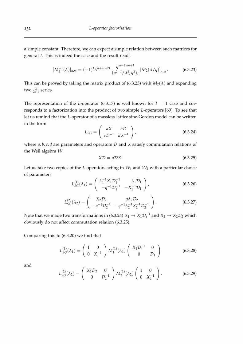
132 L-operator factorisation
a simple constant. Therefore, we can expect a simple relation between such matrices forgeneral I. This is indeed the case and the result reads
[M−12 (λ)]n,m = (−1)Iλn+m−2I qm−2mn+I
(q2−I/λ2; q2)I[M2(λ/q)]n,m . (6.3.23)
This can be proved by taking the matrix product of (6.3.23) with M2(λ) and expandingtwo φ2 1 series.
The representation of the L-operator (6.3.17) is well known for I = 1 case and cor-responds to a factorization into the product of two simple L-operators [69]. To see thatlet us remind that the L-operator of a massless lattice sine-Gordon model can be writtenin the form
LSG =
(aX bD
cD−1 dX−1
), (6.3.24)
where a, b, c, d are parameters and operators D and X satisfy commutation relations ofthe Weil algebraW
XD = qDX. (6.3.25)
Let us take two copies of the L-operators acting inW1 andW2 with a particular choiceof parameters
L(1)SG(λ1) =
(λ−1
1 X1D−11 λ1D1
−q−1D−11 −X−1
1 D1
), (6.3.26)
L(2)SG(λ2) =
(X2D2 qλ2D2
−q−1D−12 −q−1λ−1
2 X−12 D
−12
). (6.3.27)
Note that we made two transformations in (6.3.24) X1 → X1D−11 and X2 → X2D2 which
obviously do not affect commutation relation (6.3.25).
Comparing this to (6.3.20) we find that
L(1)SG(λ1) =
(1 00 X−1
1
)M(1)
1 (λ1)
(X1D−1
1 00 D1
)(6.3.28)
and
L(2)SG(λ2) =
(X2D2 0
0 D−12
)M(1)
2 (λ2)
(1 00 X−1
2
). (6.3.29)

§6.3 A trigonometric factorization 133
For the product of two L-operators (6.3.28-6.3.29) acting inW1 ⊗W2 we obtain
L(λ) = L(1)SG(λ1)L(2)
SG(λ2) =
=
(1 00 X−1
1
)M(1)
1 (λ1)
(X1X2D−1
1 D2 00 D1D−1
2
)M(1)
2 (λ1)
(1 00 X−1
2
). (6.3.30)
It is easy to check that the L-operator (6.3.30) commutes with the product X = X1X2 anddepends only on the combination D = D−1
1 D2 of the operators D1,2. Therefore, (6.3.30)nontrivially acts in the factor algebra W = W1 ⊗W2/IX where IX is the two-sideideal spanned by X = X1X2 (X obviously commutes with D). Defining the operatorsZ = X1 ≡ X−1
2 and D = D−11 D2 onW we obtain
DZ = qZD (6.3.31)
and (6.3.30) reproduces the factorization formula (6.3.17) for I = 1.
The factorization (6.3.30) of the L-operator into two simpler L-operators dependingon λ1 and λ2 has a similar form to the BLZ factorization of the transfer-matrix acting inthe Verma module VJ into the product of Q-operators [44; 45]. However, their structureis completely different, and we believe it is more closely related to the factorisation ofchapter 5. Although both factorizations produce the same L-operator, the L-operatorsL(1,2)
SG (λ1,2) in (6.3.28-6.3.29) do not act invariantly in the Verma module V+J . Due to
the presence of the operators X±11,2 they will act in the module generated by zj with j
running from −∞ to +∞. This causes trouble with a proper definition of traces. Theonly possible resolution of this problem is a restriction to the cyclic case qN = 1. Thenall representations become finite-dimensional and well defined [69].
The BLZ approach is very different in this respect. It allows to derive the Uq(sl2)L-operator in terms of the q-oscillator L-operators acting in the space spanned by zj,j = 0, . . . , ∞. A factorization of the L-operator is more involved in this case [70; 71].
Finally we would like to compare our trigonometric factorization formula (6.3.17) witha similar result obtained in [12] for the case of modular double. Unfortunately, no directcomparison is possible since the authors of [12] calculated the L-operator for a specialcase of modular representations. However, there is an explicit transformation betweenour function M2(λ) and their analog M(I) (defined after the formula (37) in [12]) whichwe denote as M(I)
CD(U). Namely, we checked that
M(I)CD(U)n,m = (−1)nU I−2nqn+Im/2−2mn[M2(U−2q−I/2)]n,m. (6.3.32)
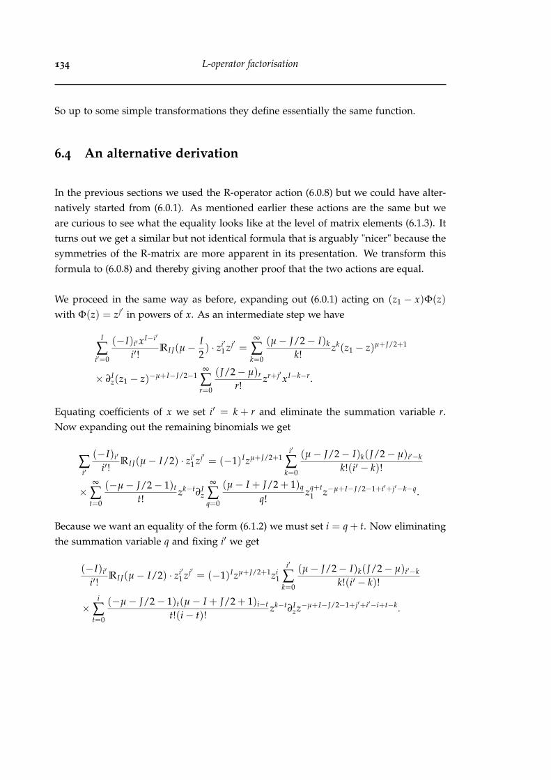
134 L-operator factorisation
So up to some simple transformations they define essentially the same function.
6.4 An alternative derivation
In the previous sections we used the R-operator action (6.0.8) but we could have alter-natively started from (6.0.1). As mentioned earlier these actions are the same but weare curious to see what the equality looks like at the level of matrix elements (6.1.3). Itturns out we get a similar but not identical formula that is arguably "nicer" because thesymmetries of the R-matrix are more apparent in its presentation. We transform thisformula to (6.0.8) and thereby giving another proof that the two actions are equal.
We proceed in the same way as before, expanding out (6.0.1) acting on (z1 − x)Φ(z)with Φ(z) = zj′ in powers of x. As an intermediate step we have
I
∑i′=0
(−I)i′xI−i′
i′!RI J(µ−
I2) · zi′
1 zj′ =∞
∑k=0
(µ− J/2− I)k
k!zk(z1 − z)µ+J/2+1
× ∂Iz(z1 − z)−µ+I−J/2−1
∞
∑r=0
(J/2− µ)r
r!zr+j′xI−k−r.
Equating coefficients of x we set i′ = k + r and eliminate the summation variable r.Now expanding out the remaining binomials we get
∑i′
(−I)i′
i′!RI J(µ− I/2) · zi′
1 zj′ = (−1)Izµ+J/2+1i′
∑k=0
(µ− J/2− I)k(J/2− µ)i′−k
k!(i′ − k)!
×∞
∑t=0
(−µ− J/2− 1)t
t!zk−t∂I
z
∞
∑q=0
(µ− I + J/2 + 1)q
q!zq+t
1 z−µ+I−J/2−1+i′+j′−k−q.
Because we want an equality of the form (6.1.2) we must set i = q + t. Now eliminatingthe summation variable q and fixing i′ we get
(−I)i′
i′!RI J(µ− I/2) · zi′
1 zj′ = (−1)Izµ+J/2+1zi1
i′
∑k=0
(µ− J/2− I)k(J/2− µ)i′−k
k!(i′ − k)!
×i
∑t=0
(−µ− J/2− 1)t(µ− I + J/2 + 1)i−t
t!(i− t)!zk−t∂I
zz−µ+I−J/2−1+j′+i′−i+t−k.

§6.4 An alternative derivation 135
Finally applying the differential operator, simplifying pochammer expressions and shift-ing back the spectral parameter we obtain the formula
[RI J(µ)]i′,j′
i,j = δi+j,i′+j′(−1)i+i′
i!(−I)i′
× ∑k,t=0
(−i,−µ− I+J2 − 1)t(−i′, µ− I+J
2 )k(µ + J−I2 + 1− j + k− t)I
t!k!(−µ + I−J2 )t−i(µ + I−J
2 + 1)k−i′. (6.4.1)
This double sum expression terminates after finitely many terms by the indices i andi′. Though the arguments are different to (6.1.3) it has a similar form. We expect thatsince the actions (6.0.1) and (6.0.8) are equal that the two formulae (6.4.1) and (6.1.3) areequal. Indeed they are, and this is pretty easy to show.
First we note an interesting feature of the summation in (6.4.1); each summation vari-able k, t yields a balanced and terminating 3F2 hypergeometric series. These series aresummable using the Pfaff-Saalschütz’s theorem (A.2.3) and we can apply it to the sumin t with n = i or in k with n = i′. It turns out either choice gives 4F3 functions that ap-pear elsewhere in this thesis. If we choose the latter, and simplify pochammer symbolswe get exactly the formula (6.1.10) multiplied by the factor C(µ; I, J) (6.1.5) which wasan intermediate step in proving (6.1.6) is the same as (3.8.5). This proves (6.4.1) is equalto (6.1.3) and equal to (3.8.5) up to normalisation (6.1.5).
If we choose to sum up the series in t instead, we get exactly the formula (3.7.7) withall i, j and I, J swapped and again multiplied by (6.1.5). The swapping of indices is justthe symmetry (3.7.21a) so they are equal.
6.4.1 q-deformation
We may find the q-deformation of (6.4.1) in the same way as we found the deformation(6.2.5) of (6.1.6). We start from (6.2.1) and rather than introducing another summationby the reverse q-Chu-Vandemonde sum (6.2.2) we instead reverse using the q-Pfaff-Saalschütz’s theorem (B.2.3). This reversal is encapsulated in the identity
(q2j−2J , λ−2qI−J+2j−2i′ ; q2)t(q2j−2i′−2J , λ−2q−I−J+2j, λ−2qI−J−2i; q2)i(q−2J ; q2)j
(q−2J+2j−2i′ ; q2)t
=(λ2q2+J−I , λ−2q−I−J+2j; q2)i(λ
−2qI−J ; q2)j+t(λ−2qJ−I ; q2)i′(q−2J ; q2)i+j−i′
(−1)iλ2(i−i′)qi2+i′(I+J)+i(J−I+1)(q−2I ; q2)i′(λ−2qI−J ; q2)j−i′

136 L-operator factorisation
× 3φ2
(q−2i′ λ2q−I−J λ2q2+I+J−2j−2t
λ2q2+I−J−2i′ λ2q2+J−I−2j−2t
∣∣∣∣∣ q2, q2
). (6.4.2)
We have written it so that all terms on the left hand side of this identity appear in theexpression (6.2.1); the variable t is the summation variable of the 4φ3 series. Thereforethe right hand side can be directly substituted, and after some simple q-pochammertransforms we obtain
[RI J(λ)]i′,j′
i,j = δi+j,i′+j′(−1)i+i′λi−i′qi−i′+I(j−i−i′)+Ji+i(i−j)+i′(i+j)
(q2; q2)i(q−2I ; q2)i′(λ2q2+J−I ; q2)I
× ∑k,t=0
(q−2i, λ−2q−2−I−J ; q2)t(q−2i′ , λ2q−I−J ; q2)k(λ2q2+J−I−2j+2k−2t; q2)I
(q2; q2)t(q2; q2)k(λ−2qI−J ; q2)t−i(λ2q2+I−J ; q2)k−i′q2k+2t(I+1).
(6.4.3)
Since we started from (6.2.1) - the q-deformation of (6.1.10) - which is equal to (6.4.1)up to normalisation (6.1.5), the formula (6.4.3) is the q-deformation of (6.4.1) up tonormalisation
Cq(λ; I, J) = (λ2q2+J−I ; q2)I
which appears in the denominator outside the sum of (6.4.3) and can be removed sothat (6.4.1) will be recovered in the limit q→ 1.
It is possible to reverse the arguments in going from (6.0.3) to (6.4.1) to obtain an op-erator action that yields (6.4.3). The reverse direction is not much more complicatedthan the forward direction, with binomial factors and theorem replaced with their qversions. The only added extra complexity are the extra q phase factors inside thesummation and the product outside which mix indices in the quantum and auxiliaryspaces. Fortunately, any problem terms can be removed without affecting the Yang-Baxter equation - they are essentially similarity and gauge transforms of the operatorwhich drop out of the equation. There are also extra phase terms appearing dependingon how we define the q-derivative. All of these considerations allow for some degree offreedom for the formula we start from and the generating function for the action thatwe obtain. We start from (6.4.3) and make the necessary transformations a posteriori bydefining RI J(λ) by
[RI J(λ)]i′,j′
i,j =(−1)Iλi−i′−Iq2(i−i′)(I−J)(λ2q2+J−I ; q2)I
q(i−i′)(i′−j)+I J/2−I/2(1− q2)I[RI J(λ)]
i′,j′
i,j . (6.4.4)
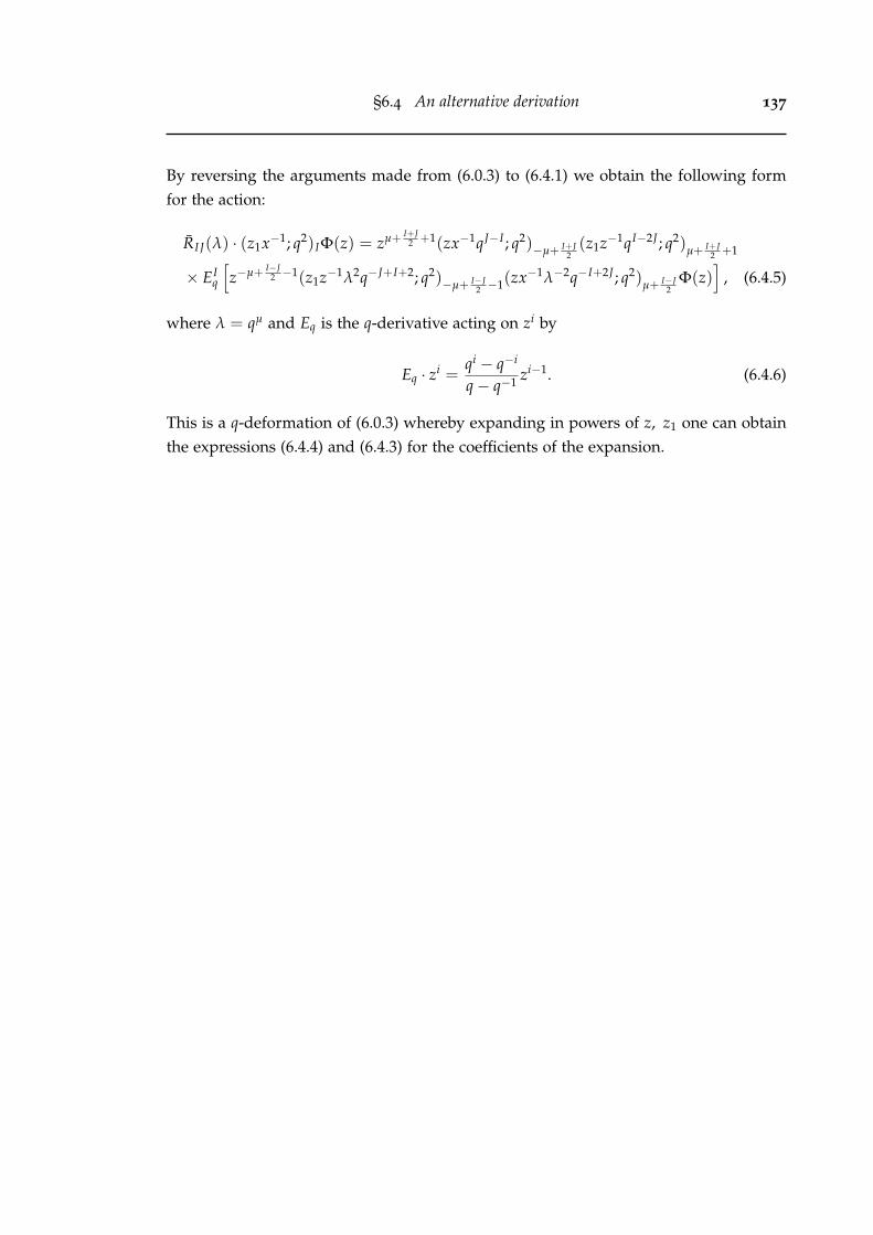
§6.4 An alternative derivation 137
By reversing the arguments made from (6.0.3) to (6.4.1) we obtain the following formfor the action:
RI J(λ) · (z1x−1; q2)IΦ(z) = zµ+ I+J2 +1(zx−1qJ−I ; q2)−µ+ I+J
2(z1z−1qI−2J ; q2)
µ+ I+J2 +1
× EIq
[z−µ+ I−J
2 −1(z1z−1λ2q−J+I+2; q2)−µ+ I−J2 −1(zx−1λ−2q−I+2J ; q2)
µ+ I−J2
Φ(z)]
, (6.4.5)
where λ = qµ and Eq is the q-derivative acting on zi by
Eq · zi =qi − q−i
q− q−1 zi−1. (6.4.6)
This is a q-deformation of (6.0.3) whereby expanding in powers of z, z1 one can obtainthe expressions (6.4.4) and (6.4.3) for the coefficients of the expansion.

138 L-operator factorisation

Chapter 7
SU(2)-invariance and coherent stateaction
In this chapter we consider the SU(2)-invariant R-matrix derived using Sklyanin’s work[15]. His construction is a solution to the additive Yang-Baxter equation
R12(u)R13(u + v)R23(v) = R23(v)R13(u + v)R12(u) (7.0.1)
acting on a tensor product V1 ⊗ V2 of finite-dimensional irreducible unitary represen-tation spaces of the group SU(2). Each Vi is realised as the space of polynomials in zi
of degree at most 2li ∈ Z+. It turns out this R-matrix is same as (3.7.7) constructed byprojecting out the solution (3.2.13) of the tetrahedron equation (and therefore the sameas the other constructions in this thesis). We will prove this by constructing an expres-sion for the matrix elements of Sklyanin’s solution for the operator action and give thetransformation of this expression to (3.7.7). In the same way as in section 6.2 of chapter6 we will also find a q-deformation of the solution in terms of its matrix elements anda generating function for its action.
First we begin with the standard definition of the Lie group SU(2) as
SU(2) = g =
(a bc d
)| a, b, c, d ∈ C, det(g) = 1, g†g = 1. (7.0.2)
The representations of this group we denote by Tli , act on elements P(zi) ∈ Vi by
Tli(g) · P(zi) = (bzi + d)2lj P(g · zi), g · zi =azi + cbzi + d
(7.0.3)
139

140 SU(2)-invariance and coherent state action
The R-operator R(λ) is constructed by considering the element
eli ,zi(zi) := (1 + zizi)2li ∈ Vi, (7.0.4)
where zi is an auxiliary parameter. This is the ‘coherent state’ with respect to the innerproduct
〈P|Q〉 = 12i
∫C
P(zi)Q(zi)µ(zi, zi)dzi ∧ dzi (7.0.5a)
µ(zi, zi) =2lj + 1
π(1 + zizi)−2(li+1)(7.0.5b)
on Vi and by which Tli(g) act as unitary operators. The inner product also has a repro-ducing kernel Eli(zi, zi) given by
P(zi) =12i
∫CEli(zi, α)P(α)µ(α, α)dαi ∧ dαi, (7.0.6)
Eli(zi, zi) = eli ,zi(zi), (7.0.7)
which is essentially a Bergman kernel as it is known in the literature [72].
The action of R(λ) on the coherent state el1,z1(z1)el2,z2(z2) ∈ V1 ⊗V2 we write as
(R(λ) · ez1 ez2)(z1, z2)
E1(z1, z1)E2(z2, z2)= R(z1, z2; z1, z2) (7.0.8)
with R the generating function of the action. The key insight into this construction bySklyanin was to notice that this generating function is a function of only one variable.This follows from SU(2) invariance of the R-operator
R12(z1, z2; z1, z2) = R12(g · z1, g · z2; (g−1)t · z1, (g−1)t · z2)
because of the existence of only one unique non-trivial SU(2)-invariant on the spaceV1 ⊗V2 given by
ξ(z1, z2; z1, z2) =(1 + z1z2)(1 + z2z1)
(1 + z1z1)(1 + z2z2), (7.0.9)
and therefore R must be a polynomial of ξ. By solving a RLL-relation for R(λ) of thesame form as (5.1.1) (with m = 2) it can be computed that R(ξ) satisfies the hypergeo-

141
metric equation
ξ(1− ξ)R′′+ [c− (1 + a + b)ξ] R
′ − abR = 0
with
a = −2l1, b = −2l2, c =λ
η+ (1− l1 − l2)
whose solution is the Jacobi polynomial
R(λ, ξ) = F2 1
(−2l1, −2l2λη − l1 − l2 + 1
∣∣∣∣ ξ
). (7.0.10)
This equation along with (7.0.8) allows us to calculate the action of R on basis elementszi′
1 zj′2 and hence deduce explicit matrix elements [R(λ)]i
′,j′
i,j by noting the relation
R(λ) · zi′1 zj′
2 = ∑i,j
[R(λ)]i′,j′
i,j zi1zj
2. (7.0.11)
Putting together (7.0.8) and (7.0.10) and making frequent use of the binomial theorem(A.2.1) we find (as an intermediate step)
∑i′,j′=0
(2l1i′
)(2l2j′
)(R(λ) · zi′
1 zj′2 )z1
i′z2j′ = ∑
n,mi=0
(2l1 − n
m1
)(2l2 − n
m2
)(n
m3
)(n
m4
)
× (2l1)!(2l2)!n!(2l1 − n)!(2l2 − n)!
n−1
∏s=0
(z1z1)m1(z2z2)m2
λ− (l1 + l2 − s− 1)η(7.0.12)
with binomial coefficients terminating each summation. Observing that the action ofR(λ) is a function of z1 and z2 only we can consider the above equation as a generatingfunction for the action in the auxiliary variables z1 and z2. In particular, the coefficientof z1
i′z2j′ gives the action of R(λ) on the basis element zi′
1 zj′2 in V1 ⊗V2. This coefficient
can easily be found by placing the constraints
i′ = m1 + m4, j′ = m2 + m3 (7.0.13)
which removes two summations on each side in (7.0.12) yielding
R(λ) · zi′1 zj′
2 =
(2l1i′
)−1(2l2j′
)−1
∑n,m1,m2=0
(2l1 − n
m1
)(2l2 − n
m2
)(n
j′ −m2
)(n
i′ −m1
)
× (2l1)!(2l2)!n!(2l1 − n)!(2l2 − n)!
n−1
∏s=0
zm1+j′−m21 zm2+i′−m1
2λ− (l1 + l2 − s− 1)η
(7.0.14)

142 SU(2)-invariance and coherent state action
as the action on the R-matrix on the basis elements. It can be seen that (7.0.14) is of thesame form as (7.0.11) by defining
i := m1 + j′ −m2, j := m2 + i′ −m1. (7.0.15)
We also observe the conservation law
i + j = i′ + j′
and the following double sum formula for R(λ):
[R(λ)]i′,j′
i,j = δi+j,i′+j′
(2l1i′
)−1(2l2j′
)−1
∑n,m2=0
(2l1 − n
m2 + i− j′
)(2l2 − n
m2
)(n
j′ −m2
)(n
j−m2
)
× (2l1)!(2l2)!n!(2l1 − n)!(2l2 − n)!
n−1
∏s=0
1λ− (l1 + l2 − s− 1)η
. (7.0.16)
Finally, after some simplification using Pochhammer identities and making the identi-fication
I = 2l1, J = 2l2,
between Sklyanin’s spin notation l1, l2 and our weight notation I, J one can easilyrewrite this formula as
[R(λ)]i′,j′
i,j = δi+j,i′+j′(−1)i−i′ i′!(−I)i−j′
j!(−I)i′(−J)j′
×∑s,l
s!(−j)l(−j′)l(−J)s+l(i− j′ − I)s+l
(λη −
I+J2 + 1)st!(l + i− j′)!(l + s− j)!(l + s− j′)!
(7.0.17)
where 0 ≤ l ≤ Min(j, j′) and 0 ≤ s ≤ J − l. For η = 1 this expression produces thesame output as (3.7.7) and (3.8.5) up to a factor B(λ; I, J) such that
[R(2),r
I,J (λ)]i′,j′
i,j= B(λ; I, J) [R(λ)]i
′,j′
i,j , (7.0.18a)
B(λ; I, J) =(λ− J
2 −I2 + 1)I
(λ + J2 −
I2 + 1)I
. (7.0.18b)
The expression (7.0.17) is yet another formula for a rational R-matrix, and has quitedifferent structure to other double sum expressions (6.0.8), (6.4.1) and (3.3.18) foundusing other methods. Regardless, in the next section we will show they are equal.

143
7.0.1 Transformation to a single sum
In applying the identities of Appendix A to the expressions in this section the argu-ments of the hypergeometric functions are already written in the correct ordering.
At first glance it appears that (7.0.17) is an unbalanced 4F3 hypergeometric series in eachsummation index and therefore difficult to transform with single sum identities. How-ever, the expression simplifies to two 3F2 series with the change of variables r := s + land eliminating s. Bringing the series in l forward the expression can be written as
[R(λ)]i′,j′
i,j = δi+j,i′+j′(−1)ji′!(−I)i−j′
i!j!(−I)i′(−J)j′(7.0.19)
×J
∑r=0
(−J)r(i− j′ − I)r
(r− j)!(λ− I2 −
J2 + 1)r
3F2
(−j′; −j −λ + I
2 +J2 − r
−r 1 + i− j′
∣∣∣∣∣ 1
)
Applying the identity (A.2.14) with n = j′, m = i the 3F2 the expression becomes
[R(λ)]i′,j′
i,j = δi+j,i′+j′(−1)i′(−I)i−j′
i!(−I)i′(−J)j′(λ− I2 −
J2 + 1)i−j′
×J
∑r=0
(−J, i− j′ − I)r
(r− j)!(λ− I2 −
J2 + 1 + i− j′)r
3F2
(−i; −i′ −λ + I
2 +J2 − i− j
−i− j 1− i− j + r
∣∣∣∣∣ 1
).
(7.0.20)
Note the change in regularisation with respect to j′ in (7.0.19) to i in (7.0.20). Observingthe summation in r we notice that it is now also a 3F2 hypergeometric series. To see thismore clearly, we rewrite (7.0.20) as
[R(λ)]i′,j′
i,j = δi+j,i′+j′(−1)i−i′(−I)i−j′Γ(λ− I
2 −J2 + 1)(1 + j)i
i!(−I)i′(−J)j′
×i
∑l=0
(−i,−i′,−λ + I2 +
J2 − i− j)l
l!(−i− j)l3F2
(1 −J i− I − j′
1− i− j + l λ− I2 −
J2 + 1 + i− j′
∣∣∣∣∣ 1
).
(7.0.21)
Note the change in regularisation used. This 3F2 hypergeometric series can be summedup using (A.2.15) with n = i + j− l, which is always positive because l runs from 0 toMin(i, i′). Summing up we obtain
[R(λ)]i′,j′
i,j = δi+j,i′+j′(−1)i (−J)j(−λ + I2 −
J2 )j−i′(λ− I
2 +J2 + 1)I
i!(−J)j′(−λ− I2 −
J2 )i+j(λ− I
2 −J2 + 1)I
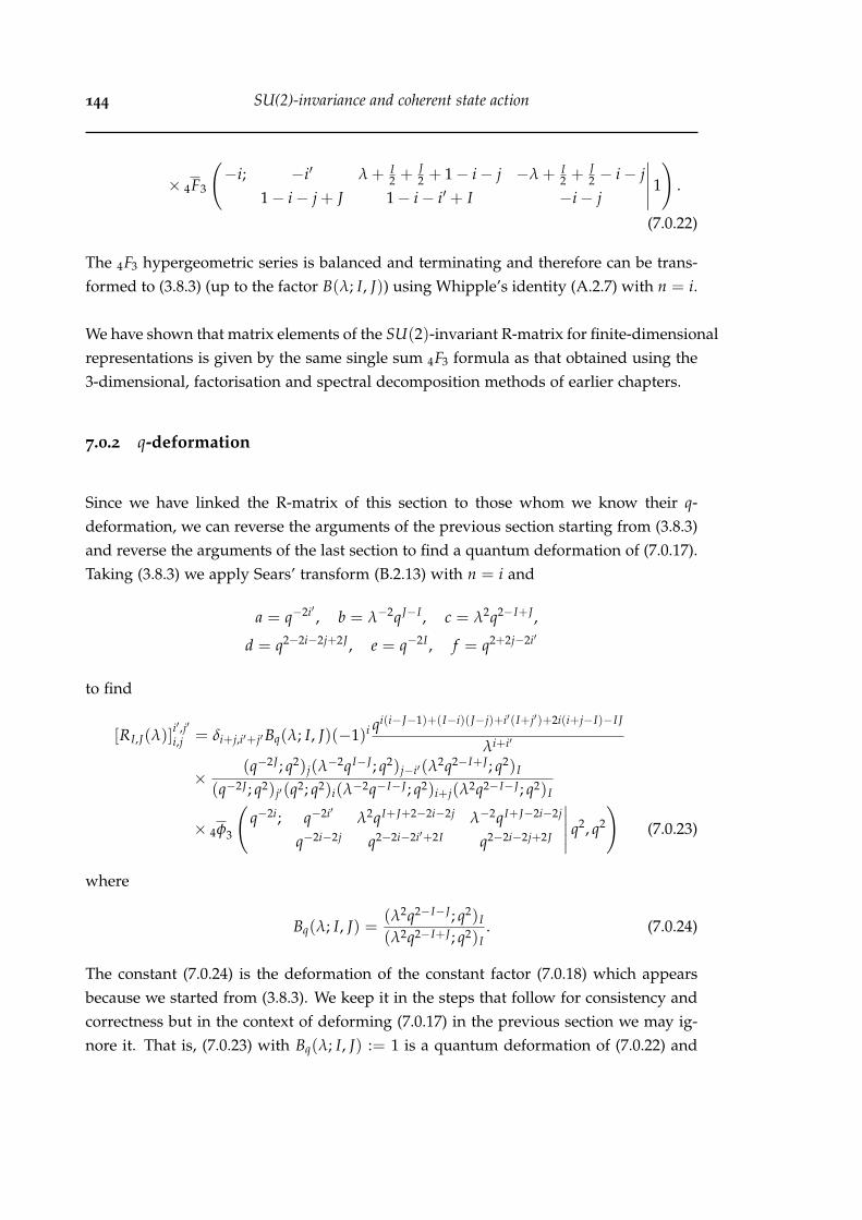
144 SU(2)-invariance and coherent state action
× 4F3
(−i; −i′ λ + I
2 +J2 + 1− i− j −λ + I
2 +J2 − i− j
1− i− j + J 1− i− i′ + I −i− j
∣∣∣∣∣ 1
).
(7.0.22)
The 4F3 hypergeometric series is balanced and terminating and therefore can be trans-formed to (3.8.3) (up to the factor B(λ; I, J)) using Whipple’s identity (A.2.7) with n = i.
We have shown that matrix elements of the SU(2)-invariant R-matrix for finite-dimensionalrepresentations is given by the same single sum 4F3 formula as that obtained using the3-dimensional, factorisation and spectral decomposition methods of earlier chapters.
7.0.2 q-deformation
Since we have linked the R-matrix of this section to those whom we know their q-deformation, we can reverse the arguments of the previous section starting from (3.8.3)and reverse the arguments of the last section to find a quantum deformation of (7.0.17).Taking (3.8.3) we apply Sears’ transform (B.2.13) with n = i and
a = q−2i′ , b = λ−2qJ−I , c = λ2q2−I+J ,
d = q2−2i−2j+2J , e = q−2I , f = q2+2j−2i′
to find
[RI,J(λ)]i′,j′
i,j = δi+j,i′+j′Bq(λ; I, J)(−1)i qi(i−J−1)+(I−i)(J−j)+i′(I+j′)+2i(i+j−I)−I J
λi+i′
×(q−2J ; q2)j(λ
−2qI−J ; q2)j−i′(λ2q2−I+J ; q2)I
(q−2J ; q2)j′(q2; q2)i(λ−2q−I−J ; q2)i+j(λ2q2−I−J ; q2)I
× 4φ3
(q−2i; q−2i′ λ2qI+J+2−2i−2j λ−2qI+J−2i−2j
q−2i−2j q2−2i−2i′+2I q2−2i−2j+2J
∣∣∣∣∣ q2, q2
)(7.0.23)
where
Bq(λ; I, J) =(λ2q2−I−J ; q2)I
(λ2q2−I+J ; q2)I. (7.0.24)
The constant (7.0.24) is the deformation of the constant factor (7.0.18) which appearsbecause we started from (3.8.3). We keep it in the steps that follow for consistency andcorrectness but in the context of deforming (7.0.17) in the previous section we may ig-nore it. That is, (7.0.23) with Bq(λ; I, J) := 1 is a quantum deformation of (7.0.22) and

145
so forth in the steps that follow.
Next we reintroduce the second summation by expanding out factors in (7.0.23) us-ing identity (B.2.21) with
n = I + j− i′, m = i + j− l,
b = q−2J , e = λ2q2−I−J−2j+2i′
where we denote by l the summation index of the 4φ3 series. l runs from 0 to Min(i, i′)so n ≥ m and so the identity can safely be used. In particular,
(λ2qJ+I+2−2i−2j; q2)l(λ2qJ−I+2; q2)I(λ
−2qI−J ; q2)j−i′(q−2J ; q2)j
(q2J−2j−2i+2; q2)l(λ−2q−I−J ; q2)i+j=
qi′−j+j2+i′2−2ji′
(q2; q2)I+j−i′
× q−J(i+i′)+I(i+2j−i′)+2I J
(q−2J+2j; q2)i3φ2
(q−2I−2j+2i′ ; q−2J q2
q2−2i−2j+2l λ2q2−I−J−2j+2i′
∣∣∣∣∣ q2, q2
). (7.0.25)
We have written the identity so that all terms on the left hand side appear in (7.0.23)and so we can substitute them for the right hand side directly. Combining (7.0.23) and(7.0.25) we have the double sum expression
[RI,J(λ)]i′,j′
i,j = δi+j,i′+j′Bq(λ; I, J)(−1)i−i′λi+i′q−j−j′+i2−ij+ii′+ji′−I(i+j)−J(i+i′)+2I J
(λ2q2−I−J ; q2)I
×(q−2I ; q2)i−j′
(q−2I ; q2)i′(q−2J ; q2)j′
[i + j
i
]q2
i
∑l=0
q2l (q−2i, q−2i′ , λ−2qI+J−2i−2j; q2)l
(q2, q−2i−2j; q2)l(q2; q2)l+I−i−i′
× 3φ2
(q−2I−2j+2i′ ; q−2J q2
q2−2i−2j+2l λ2q2−I−J−2j+2i′
∣∣∣∣∣ q2, q2
). (7.0.26)
Now rewriting (7.0.26) by identifying the 3φ2 hypergeometric series indexed by ‘l’ wehave
[RI,J(λ)]i′,j′
i,j = δi+j,i′+j′Bq(λ; I, J)(−1)jλj+j′q−j+i2+j′2+ij+ii′+ji′(q−2I ; q2)i−j′(λ
−2qI+J ; q2)j−i′
q2jj′−2i′ j′+I(j+j′)+J(i+j)−2I J(q−2I ; q2)i′(q−2J ; q2)j′(q2; q2)i
×J
∑r=0
q2r(q−2I−2j+2i′ , q−2J ; q2)r
(λ2q2−I−J−2j+2i′ ; q2)r(q2; q2)r−j3φ2
(q−2i; q−2i′ λ−2qI+J−2i−2j
q−2i−2j q2−2i−2j+2r
∣∣∣∣∣ q2, q2
),
(7.0.27)

146 SU(2)-invariance and coherent state action
analogous to (7.0.20). Now reversing the transformation (7.0.19) to (7.0.20) using iden-tity (B.2.23) on the 3φ2 function with n = i, m = j′ we have
[RI,J(λ)]i′,j′
i,j = δi+j,i′+j′Bq(λ; I, J)qi′ j′−ij−J(i+j)−I(j+j′)+2I J+j(j−1)(q2; q2)i′(q−2I ; q2)i−j′
(−1)jλ−j−j′(q−2I ; q2)i′(q−2J ; q2)j′(q2; q2)i(q2; q2)j
×J
∑r=0
q2r+2rj′(q−2I−2j+2i′ ; q2)r(q−2J ; q2)r
(λ2q2−I−J ; q2)r(q2; q2)r−j3φ2
(q−2j′ ; q−2j λ−2qI+J−2r
q−2r q2−2j+2i′
∣∣∣∣∣ q2, q2
)(7.0.28)
which deforms (7.0.19). Finally we reverse the change of summation index introducedin transforming (7.0.17) to (7.0.19) by defining r := s + l and eliminating r. We thenrewrite the double sum by removing the nested summation implicit in the 3φ2 series(and whose summation variable is l). We also remove the inessential constant factorBq(λ; I, J) that only appears because we started from (3.8.3). Finally we see that (7.0.28)can be rewritten as
[R(λ)]i′,j′
i,j = δi+j,i′+j′qi2−i(I−j+J+i′+1)−2I j+2I J+Ii′+2j2−jJ−ji′−2j+i′(q2; q2)i′(q−2I ; q2)i−j′
(−1)i′−iλi′−i−2j(q2; q2)j(q−2I ; q2)i′(q−2J ; q2)j′
×∑s,l
λ−2lql(I+J+2)+2s+2l(q2; q2)s(q−2j, q−2j′ ; q2)l(q−2J , q2i−2I−2j′ ; q2)s+l
(q2; q2)l(q2; q2)i+l−j′(q2; q2)s+l−j(q2; q2)s+l−j′(λ2q−I−J+2; q2)s(7.0.29)
with summation variables running over the same values as its rational limit (7.0.17)whereby taking the limit of (7.0.29) as q→ 1 we obtain (7.0.17).
7.1 Generating function for q-action
In this section we will continue reversing the arguments of the last section to find aq-deformation of R(ξ). It is interesting to see whether the generating function still re-mains a function of a single variable. Unfortunately, this does not appear to be the case.Instead, the 2F1 expression in (7.0.10) becomes a balanced and terminating 4φ3 function.
The main problem we have is defining the q-analogue of the functions eli ,zi(zi) andEli(zi, zi). These functions have special properties as coherent states and reproducingkernels with respect to the inner product (7.0.5) on the SU(2) representation spacesconsidered in this chapter. As far as we are aware, this theory in the case of quantumgroups is not completely known. Some work has been done in this area, and the notionof a q-coherent state qezi(zi) was proposed in [73] which we will use in our calculations.

§7.1 Generating function for q-action 147
Let us define
qezi(zi) := (−ziziq1−2li ; q2)2li (7.1.1a)
qE(zi, zi) := (−ziziq1−2li ; q2)2li (7.1.1b)
2l1 := I, 2l2 := J (7.1.1c)
In our calculations we make frequent use of the q-binomial theorem (B.2.1b) in thesame way we labelled expressions Ck
n in (7.0.12) the same pochammer symbols appearin (7.0.29) as q-pochammer symbols. That is, starting from (7.0.29) (with Bq(λ; I, J) := 1)and reversing arguments we get the intermediate step
∑i′,j′
(q−2I ; q2)i′(q−2J ; q2)j′qIi′+i′+J j′+j′
(−1)i′+j′(q2; q2)i′(q2; q2)j′R(λ) · zi′
1 zj′2 z1
i′z2j′ =
= ∑s,m1
(q2; q2)I(q2; q2)Jq2s2−2Is−2Js+2I J
(q2; q2)I−s(q2; q2)J−s(q2, λ2q2−I−J ; q2)sq2 Dm1
I−szm11 z1
m1(−1)m1 qm1−Im1−Jm1+2m1s
×∑m2
Dm2J−sz
m22 z2
m2(−1)m2 qm2−Im2−Jm2+2m2s ∑m3
q2 Dm3s λm3 zm3
1 z2m3(−1)m3 qm3−Im3
×∑m4
q2 Dm4s λm4 zm4
2 z1m4(−1)m4 qm4−Jm4 qm1m3−m2m3−m1m4+m2m4 ,
where on the right hand side we have reintroduced summation indices mi that we usedto expand out ξ (7.0.9) in the classical case and run over the same values. The rela-tion between the mi and our tensor indices are exactly the same as in the classical case(7.0.13), (7.0.15).
The phase term qm1m3−m2m3−m1m4+m2m4 is problematic because it couples the summationvariables. However, this term can be removed, because
m1m3 −m1m4 −m2m3 + m2m4 =12(i2 + j2 − i′2 − j′2
),
which is just the similarity transform (6.3.2)
RI,J(λ) = (U ⊗U)RI,J(λ)(U−1 ⊗U−1),
Umn = δn,mqn2/2
that we made in constructing the L-operator factorisation (6.3.17). As explained inchapter 6, although this gives a slightly different matrix element it does not affect theYang-Baxter equation. Therefore to uncouple the sums over mi, we from now on workwith R(λ).

148 SU(2)-invariance and coherent state action
Using the binomial theorem (B.2.1a) to sum the mi we are left with only a sum in s.After making some simplifications we obtain
Proposition 7.1.1.(R(λ) · qez1 qez2
)(z1, z2)
qE(z1, z1)qE(z2, z2)= q2I J (−z1z1q1−I−J ; q2)I(−z2z2q1−I−J ; q2)J
(−z1z1q1−I ; q2)I(−z2z2q1−J ; q2)J(7.1.2)
× 4φ3
(q−2I q−2J −z1z2λq1−I −z2z1λq1−J
λ2q2−I−J −z1z1q1−I−J −z2z2q1−I−J
∣∣∣∣∣ q2, q2
)
which is a q-deformation of (7.0.8) which we call Rq(z1, z2; z1, z2).
Because the right hand side is a balanced and terminating 4φ3 hypergeometric seriesand I, J ∈ Z+ the expression has many equivalent forms generated by the Sears’ trans-forms (B.2.13) and (B.2.14). Some of these are symmetries of Rq, and they can begenerated from three elementary ones:
Rq(z1, z2; z1, z2) = Rq(−z1,−z2;−z1,−z2), (7.1.3a)
Rq(z1, z2; z1, z2) = Rq(z1−1, z2
−1, z−11 , z−1
2 ), (7.1.3b)
Rq(λ|z1, z2; z1, z2) =q−I J
Bq(λ; I, J)Rq(λ
−1q−1|z1,−z2−1; z1,−z−1
2 ) (7.1.3c)
where Bq(λ; I, J) is given by (7.0.24).
Chapter 8
A stochastic R-matrix
In this chapter we consider the stochastic nature of the R-matrices constructed in thisthesis. It turns out that with a small modification to the phase terms in (3.3.24) thecolumns of the R-matrix related to symmetric tensor representations of Uq(sln) sum tounity. The positivity of each element follows from the positivity of the 3-dimensionalBoltzmann weights in the construction (3.3.4) and condition (3.3.17).
In the recent work of [21; 23] the Uq(sl2) R-matrix at a special value of λ was con-sidered and shown to describe the probability distribution function of a four parameterfamily of integrable stochastic zero range processes involving interacting particles on aline. For certain values of these parameters it is possible to recover many known inte-grable models in the Kardar-Parisi-Zhang universality class. A Uq(sln) generalisationΦq(γ|β; λ, µ) was constructed in [20] and is essentially the reductions (3.5.1), (3.5.2) ofour R-matrix. This is an important link in light of the factorisation (3.5.7), where wehave reconstructed the full R-matrix from its values at two special points. It appearsthat the R-matrix constructed with the 3D approach is somehow a combination of twointegrable stochastic models. In this chapter we will write the combination down ex-plicitly and use it to prove the stochasticity of the general R-matrix.
In the second part of this chapter we will propose a possible generalisation for all high-est weight representations in the case of sl3. It comes from the factor R(1)(λ) (5.6.15)constructed from Derkachov’s factorisation method. It is true that this factor in the caseof sl2 is stochastic and it appears that it may also be the case for sl3, where we haveobserved that it satisfies the sum-to-unity property. We cannot give a proof at this time,and we only present it as a possible generalisation. We wonder if it continues to holdfor sln, and if so, what kind of stochastic processes can be modeled by it.
149

150 A stochastic R-matrix
8.0.1 Symmetric tensor representations of Uq(sln)
Let us define another R-matrix SI,J(λ) by
[SI,J(λ)]i′,j′
i,j = ρi′,j′
i,j
[R(n)
I,J (λ)]i′,j′
i,j, i, j, i′, j′ ∈ Zn−1
+ , (8.0.1)
with
ρi′,j′
i,j = q[i,j]−[i′,j′]+ ∑
1≤k<l≤n(jkil−i′k j′l)
= q(i,j)−(i′,j′)−J|i|+I|j′|+ ∑
1≤k<l<n(jkil−i′k j′l)
. (8.0.2)
In [20] SI,J(z) was given in terms of RKI,J(z) with z = λ−2. Here we defined SI,J(λ) in
terms of R(n)I,J (λ) using the relation (3.6.10). Using quantum group arguments it was
shown in [20] that (8.0.1) solves the Yang-Baxter equation and satisfies the stochasticitycondition
∑i,j
[SI,J(λ)]i′,j′
i,j = 1. (8.0.3)
We can now give the direct proof of (8.0.3) using the explicit formula (3.3.24) for theR-matrix.
To do that we find it convenient to follow notations of [20]. Introduce the function
Φq(γ|β; λ, µ) = qξ(µ
λ
)|γ| (λ; q)|γ|(µλ ; q)|β|−|γ|
(µ; q)|β|
n−1
∏s=1
[βs
γs
]q, (8.0.4)
ξ = ∑1≤l<k<n
(βl − γl)γk, (8.0.5)
where α, β, γ, δ ∈ Zn−1+ , and λ, µ ∈ C. This function satisfies the sum-to-unity rule
∑i
Φq(i|j; λ, µ) = 1. (8.0.6)
Note that the sum in (8.0.6) is always finite since the summand is equal to zero unless0 ≤ i ≤ j, i.e. 0 ≤ is ≤ js for all s = 1, . . . , n− 1. The relation (8.0.6) can be easily provedby induction in n, see [20] for details.
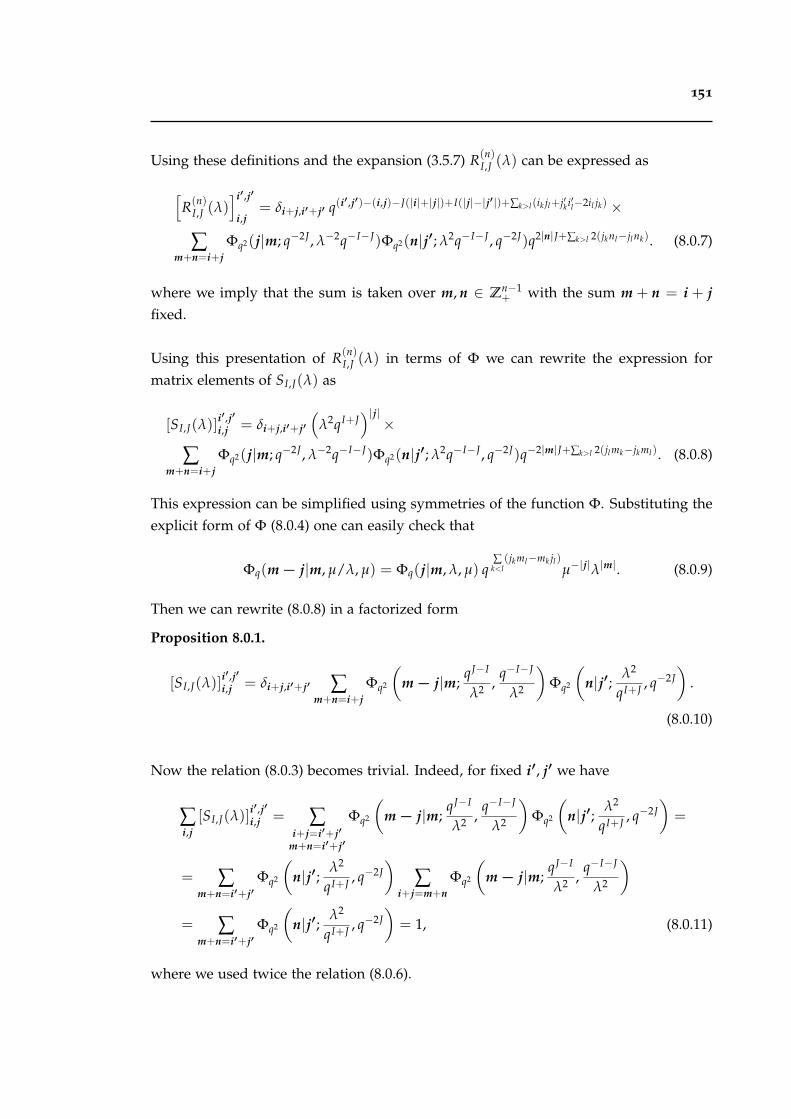
151
Using these definitions and the expansion (3.5.7) R(n)I,J (λ) can be expressed as
[R(n)
I,J (λ)]i′,j′
i,j= δi+j,i′+j′ q(i
′,j′)−(i,j)−J(|i|+|j|)+I(|j|−|j′|)+∑k>l(ik jl+j′ki′l−2il jk) ×
∑m+n=i+j
Φq2(j|m; q−2J , λ−2q−I−J)Φq2(n|j′; λ2q−I−J , q−2J)q2|n|J+∑k>l 2(jknl−jlnk). (8.0.7)
where we imply that the sum is taken over m, n ∈ Zn−1+ with the sum m + n = i + j
fixed.
Using this presentation of R(n)I,J (λ) in terms of Φ we can rewrite the expression for
matrix elements of SI,J(λ) as
[SI,J(λ)]i′,j′
i,j = δi+j,i′+j′(
λ2qI+J)|j|×
∑m+n=i+j
Φq2(j|m; q−2J , λ−2q−I−J)Φq2(n|j′; λ2q−I−J , q−2J)q−2|m|J+∑k>l 2(jlmk−jkml). (8.0.8)
This expression can be simplified using symmetries of the function Φ. Substituting theexplicit form of Φ (8.0.4) one can easily check that
Φq(m− j|m, µ/λ, µ) = Φq(j|m, λ, µ) q∑
k<l(jkml−mk jl)
µ−|j|λ|m|. (8.0.9)
Then we can rewrite (8.0.8) in a factorized form
Proposition 8.0.1.
[SI,J(λ)]i′,j′
i,j = δi+j,i′+j′ ∑m+n=i+j
Φq2
(m− j|m;
qJ−I
λ2 ,q−I−J
λ2
)Φq2
(n|j′; λ2
qI+J , q−2J)
.
(8.0.10)
Now the relation (8.0.3) becomes trivial. Indeed, for fixed i′, j′ we have
∑i,j
[SI,J(λ)]i′,j′
i,j = ∑i+j=i′+j′
m+n=i′+j′
Φq2
(m− j|m;
qJ−I
λ2 ,q−I−J
λ2
)Φq2
(n|j′; λ2
qI+J , q−2J)=
= ∑m+n=i′+j′
Φq2
(n|j′; λ2
qI+J , q−2J)
∑i+j=m+n
Φq2
(m− j|m;
qJ−I
λ2 ,q−I−J
λ2
)
= ∑m+n=i′+j′
Φq2
(n|j′; λ2
qI+J , q−2J)= 1, (8.0.11)
where we used twice the relation (8.0.6).
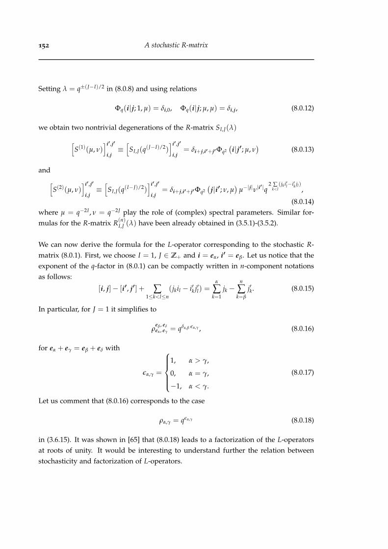
152 A stochastic R-matrix
Setting λ = q±(J−I)/2 in (8.0.8) and using relations
Φq(i|j; 1, µ) = δi,0, Φq(i|j; µ, µ) = δi,j, (8.0.12)
we obtain two nontrivial degenerations of the R-matrix SI,J(λ)[S(1)(µ, ν)
]i′,j′
i,j≡[SI,J(q(J−I)/2)
]i′,j′
i,j= δi+j,i′+j′Φq2
(i|j′; µ, ν
)(8.0.13)
and[S(2)(µ, ν)
]i′,j′
i,j≡[SI,J(q(I−J)/2)
]i′,j′
i,j= δi+j,i′+j′Φq2
(j|i′; ν, µ
)µ−|j|ν|i
′|q2 ∑
k<l(jki′l−i′k jl)
,
(8.0.14)where µ = q−2I , ν = q−2J play the role of (complex) spectral parameters. Similar for-mulas for the R-matrix R(n)
I,J (λ) have been already obtained in (3.5.1)-(3.5.2).
We can now derive the formula for the L-operator corresponding to the stochastic R-matrix (8.0.1). First, we choose I = 1, J ∈ Z+ and i = eα, i′ = eβ. Let us notice that theexponent of the q-factor in (8.0.1) can be compactly written in n-component notationsas follows:
[i, j]− [i′, j′] + ∑1≤k<l≤n
(jkil − i′k j′l) =α
∑k=1
jk −n
∑k=β
j′k. (8.0.15)
In particular, for J = 1 it simplifies to
ρeβ, eδeα, eγ = qδα,β εα,γ , (8.0.16)
for eα + eγ = eβ + eδ with
εα,γ =
1, α > γ,
0, α = γ,
−1, α < γ.
(8.0.17)
Let us comment that (8.0.16) corresponds to the case
ρα,γ = qεα,γ (8.0.18)
in (3.6.15). It was shown in [65] that (8.0.18) leads to a factorization of the L-operatorsat roots of unity. It would be interesting to understand further the relation betweenstochasticity and factorization of L-operators.

153
We can now derive the formula for the L-operators corresponding to the stochasticR-matrix SI,J(λ). Using (8.0.15) for general J and (3.6.5) one can write it in terms ofWeil generators (3.6.21) similar to (3.6.23) in a compact form
LSα,β(µ) = µεα,β X−1
α Xβ
[µδα,β Zα
] n
∏γ=1
Zεα,γγ . (8.0.19)
It satisfies the algebra
S1,2(µ/ν)LS1(µ)⊗ LS
2(ν) = LS2(ν)⊗ LS
1(µ)S1,2(µ/ν), (8.0.20)
where S1,2(λ) is given by (8.0.1) with I = J = 1. This L-operator was first obtained in[65] in a slightly different form. The root of unity condition qN = 1 used there does notaffect the local structure of the algebra (8.0.20).
Choosing the eigenvalue of the operator Z in (3.6.24) as C one can rewrite (8.0.19)as
Lα,β(µ) = µεα,β+δα,β C X−1α Xβ (1− µ−2δα,β Z−2
α )n
∏s=α+1
Z−2s . (8.0.21)
This L-operator contains two complex parameters µ and C = qJ , where J can be identi-fied with the weight of representation. As well known one can multiply the L-operator(8.0.21) by arbitrary complex parameters ai (“horizontal” fields) from the left withoutaffecting the Yang-Baxter relation. It immediately follows from the property
[A1 ⊗ A2, S1,2(µ)] = 0, (8.0.22)
where A = a1, . . . , an.
We can also remove one pair of Weyl operators Z1, X1 by setting
Z1 = Cn
∏i=2
Z−1i , X1 ≡ 1. (8.0.23)
Let us introduce another set of operators
ki = q−2Z−2i+1, φ+
i = X−1i+1(1− Z−2
i+1), φi = Xi+1, i = 1, . . . , n− 1 (8.0.24)
instead of Zi, Xi, i = 2, . . . , n. Each set ki, φi, φ+i forms a q-oscillator algebra
φk = q2kφ, φ+k = q−2kφ+, φφ+ − q2φ+φ = 1− q2. (8.0.25)

154 A stochastic R-matrix
If we now choose
a1 = −µC, ai =µvC
q2(i−1−n), i = 2, . . . , n (8.0.26)
and make a change of variables
C =
√uv
qn , µ = q√
xv
, (8.0.27)
then we get exactly the L-operator from the recent paper by Garbali, De Gier andWheeler [74]
LGGWi,j (x) = aiLi,j(µ), (8.0.28)
with Lij(µ) given by (8.0.21). Therefore, the L-operator LGGW(x) corresponds to thestandard Uq(sln) L-operator for symmetric representations in the presence of twist and“horizontal” fields.
8.0.2 Towards an arbitrary highest weight generalisation
Let us introduce a function Ψ by
Ψ(j, j′|λ1, λ2, λ3) =
=(−1)j2+j′3 j′1!(j′2 + j′3)!(λ2 − 1)j′2
(1− λ1)j3(λ1)j1−j3(λ2 − λ1)j′1+j′2−j1+j3
j1!j2!j3!(j′2 + j′3 − j2 − j3)!(j′1 − j1 − j′3 + j3)!(λ2)j′1+j′2(λ2 − λ3 − 1)j′2+j′3
×∑m,l
(−j3, λ1 + j1 − j3, λ1 − λ3 − 1)m(−j′2, 1− λ2 − j′1 − j′2, 2 + λ3 − λ2 − j′2 − j′3)l
m!l!(−j2 − j3, λ1 − j3)m(2− λ2 − j′2,−j′2 − j′3)l
× (−j2 − j3)l+m
(1 + λ1 − λ2 + j1 − j3 − j′1 − j′2)l+m(8.0.29)
with summation indices 0 ≤ m, l ≤ j2 + j3. It appears to satisfy the sum-to-unity rule
Proposition 8.0.2.
∑j
Ψ(j, j′|λ1, λ2, λ3) = 1. (8.0.30)
The sum in j = j1, j2, j3 is finite and it is easy to see that it terminates due to denomi-nator factorials such that
0 ≤ j1 ≤ j′1 + j′2 0 ≤ j2 ≤ j′2 + j′3, 0 ≤ j3 ≤ j′2 + j′3.

155
As mentioned in the introduction, Ψ is just the function for elements of R(1)(λ) (5.6.15)with relabeled variables. The relation is[
R(1)(λ)]i′,j′
i,j= δ
jiδi3,i′3
Ψ(j, j′|λ− J1,−J1, J2). (8.0.31)
For special values of Ψ we recover the rational limit of Φq for n = 3. In particular
Ψ(j, j′|λ, µ, 0) = limq→1
Φq(γ|β; λ, µ) (8.0.32)
with j = j1, j2, 0 = γ and j′ = j′1, j′2, 0 = β. Therefore the rational limit of Φq
is, up to n = 3, contained within a larger function related to arbitrary highest weightrepresentations of sl3. We expect this to be true for all n, and perhaps even in thetrigonometric case, but as of yet we have not constructed such a function.

156 A stochastic R-matrix

Chapter 9
Conclusion
In this thesis we have considered solutions to the Yang-Baxter equation related to sln.Such solutions are known as R-matrices, and we have considered five different ap-proaches to constructing them on the level of matrix elements, thereby indirectly eval-uating the universal R-matrix (2.4.50) for the symmetric tensor representations. In theprocess we have uncovered and clarified in explicit detail some of the structure of thesesolutions, and structure which is not at all obvious from the q-exponential form of theuniversal solution. It is clear that the R-matrix is a composite object, summarised in oneway by the formula
R(λ) = Φ ∗Φ (9.0.1)
detailed in (8.0.10), (8.0.4), and (3.5.6)-(3.5.8). We think this is a remarkable relation, par-ticularly for the matrix elements. Elements of the left hand side are expressible by the(n− 1)-fold sum multivariable basic hypergeometric series (3.3.24), but the elements ofΦ functions on the right hand side are simple binomial products. Moreover, the func-tions Φ are objects of great interest at the time of writing, with a recent explosion ofresearch in their application to integrable near-equilibrium stochastic models. Equation(9.0.1) is another step towards clarifying the relation these models have with the latticemodels of equilibrium statistical mechanics that we gave a brief overview of in chapter2, and where the notion of R-matrix and Yang-Baxter integrability was first formulated.The function Φ by itself defines an R-matrix (8.0.13), (8.0.14), and therefore the factori-sation of R(λ) is also a composition of ‘smaller’ R-matrices.
In chapter 3 we studied the 3-dimensional structure of the Uq(sln) R-matrix in the caseof symmetric tensor representations. The formula (3.3.4) can be considered as a traceof an operator product, graphically represented in Figure 3.4. Though the notion of aprojecting a 3-dimensional model is not new, the link between quantum groups and
157

158 Conclusion
solutions to the tetrahedron equation is a relatively recent development. It is perhapswith this approach we can claim the most success so far. We are confident that theformula (3.3.24) obtained from this approach is the simplest, and neatest formula onecould find for the R-matrix elements for these representations. We come to this conclu-sion after our investigation of other methods, where even in the case of sl2 much morework was required in obtaining the single summation formula (3.8.3). We also mentionthat (3.3.24) makes it very easy to derive the reductions (3.5.1), (3.5.2) from which wederived (9.0.1). As argued in section 3.5, they exist within (3.3.24) as a single summandwhich is easy to extract. In other presentations, they exist in a more ‘dispersed form’,and it takes more technical arguments with summation formulae to extract their for-mula.
We also note that (3.3.24) is the most general formula for the R-matrix elements cur-rently available in the literature. In fact, for the R-matrix with arbitrary weights forboth representations, it may be the only known formula. Most presentations usuallytake a fundamental representation in one or both spaces, but in our formula the weightsare arbitrary complex parameters. We matched our formula to these special cases insection 3.6, and we showed that with the right choice of normalisation a formula for thestandard Uq(sln) L-operator (3.6.5) can be given. Actually, (3.6.1) gives us an entire fam-ily of higher spin L-operators for I ∈ Z+, J ∈ C, without the need for fusion procedures.
We also remark that the symmetries of the R-matrix discussed in section 3.4 are mucheasier to see from the 3-dimensional approach compared to other methods. They man-ifest as higher dimensional symmetries of the 3-dimensional Boltzmann weights pro-jected out in one direction. It is interesting to see how transformations of the internaldegrees of freedom inside the R-matrix yield invariant transformations of the overalloperator. A similar idea also happens in chapter 5 for the factorisation (5.1.8) wherethe identity (5.3.4e) allows us to reorder the factors without affecting the R-matrix. Thesymmetries usually give different formulae but with the same output, and so they de-scribe a group of transformations of the hypergeometric series we have derived. For thespecial case of Uq(sl2) the formula (3.3.30) these symmetries are contained within thetransformation group of Sears’ transforms (B.2.13), (B.2.14) and probably the symme-tries of higher rank R-matrices are special cases of a more general yet to be discoveredidentity.
In chapter 4 we used the representation theory of quantum groups directly to con-struct the R-matrix elements in the case of Uq(sl2). We exploit the fact that a ten-sor product of irreducible finite-dimensional representations of the quantum group is

159
semisimple. The intertwining relation (4.1.7a) allows us to write down the R-matrix asa sum of projection operators onto these components, acting on each subspace by aneigenvalue (4.1.12) determined by the Jimbo equations. This approach, besides the uni-versal R-matrix, perhaps most clearly demonstrates the link between quantum groups(in their modern form) and the Yang-Baxter equation, because the solution is essentiallya special combination of Clebsch-Gordan coefficients - pure representation theoreticalobjects. One can therefore say that so is the R-matrix, and it is obvious that it is anotherstep in complexity in the heirarchy of special functions that appear in representationtheory. This fact is pretty well known, in particular that the R-matrix is closely relatedto 6j-symbols which arise when considering the decomposition of the tensor productof three irreducible representations.
The main challenge therefore is constructing the Clebsch-Gordan coefficients. In thecase of Uq(sl2) which we have considered the formula is quite well known, but it ap-pears to be a highly non-trivial and unsolved problem for quantum groups in general.Even when it is known, there are some serious limitations of the method, because itdoes not work when the representation space contains multiplicities. This rules outmany possible solutions we could construct. In the simplest case, the solution (4.2.9) isthe least elegant of all the solutions constructed in this thesis. It is a triple summationinvolving somewhat complicated hypergeometric series and it is only valid for integralweights. The tools we used to construct this formula have been known for quite sometime, yet (at least to our knowledge) it does not appear anywhere in the literature. Per-haps until (3.8.3) appeared in [10] the general higher spin R-matrix was considered toocomplicated to write down. The main result of this chapter was showing that the for-mula is not that complicated at all, and is actually equivalent to the q-Racah single sumpolynomial representation (3.8.3) obtained from the 3-dimensional approach, therebyproving these are equivalent constructions.
One surprise was the intermediate step (4.2.14) in our calculations, which allows usto write the R-matrix as (4.2.20). It is not of the same form as (4.1.9) and each factoris given by a binomial product expression and the overall expression a double summa-tion. We think the expression has a ‘nice’ form, but currently we do not know if it hasany significance.
In chapter 5 we considered the factorisation approach due to Derkachov and Man-ashov. The techniques have so far only been developed for the rational sln R-matricesbut a major appeal is the construction of the general R-matrix for any highest weightrepresentation. The components in (5.3.1) we have constructed in the case of sl2 and sl3
160 Conclusion
and we have shown how they relate to our factorisation (3.5.6) and (3.7.18). It appearsthat they are essentially the same idea, although we have not yet checked the reducedRLL-relations (5.1.9) for the q-deformation. Our factorisation is more general in thesense that it holds for trigonometric R-matrices, but (5.3.1) is more general in the sensethat it holds for more representations. We have also shown that in the restriction tosymmetric tensor representations, the equation (5.3.1) simplifies significantly into justtwo symmetrical factors and this occurs not by some factors reducing trivially but by anon-trivial operator composition.
We also considered and verified some interesting identities (5.3.4) satisfied by the ‘build-ing block’ operators R(i)(λ). For sl2 they correspond to some well known identities inthe theory of hypergeometric series. We were able to construct these expressions for sl3as well but the identities are far more complicated multivariable hypergeometric seriesand do not seem to be like anything we have encountered in the literature. This mightindicate some new identities but we have not yet paid serious attention to refining andmaking sense of them so we did not include them in this thesis. All we can say is thatthey exist and we used them to check that our expressions for the sl3 factors R(i)(λ) arecorrect.
Our initial interest in the method of chapter 5 was to find a better formula than (3.3.24)in the case of sl3. It looked promising after considering the sl2 case where the single sumformula (3.7.7) emerged immediately, but for higher rank algebras the process seems tobe far less efficient for the same representations. For example, if we want to calculatethe sl3 case for symmetric tensor representations (like we did in section 5.6.4) we needto construct the factors for arbitrary representations and then restrict afterwards. Thisis because of the way the factors intertwine the representations (as given in (5.3.2)), sothere are always contributions to the operator composition from the entire space. Theinitial formula obtained by putting these factors together is a quadruple sum but it canbe shown that this is equivalent to the double sum in (3.7.4).
In chapter 6 we considered another factorisation (6.0.6) of the R-matrix by Chicherinand Derkachov. At the time of writing, this factorisation is known for sl2 as well as thequantum and elliptic doubles in the literature. In this thesis we have generalised theresult to Uq(sl2) (6.3.17). We did this by first constructing matrix elements for their R-matrix via its action on the monomial basis of Verma modules. We then proved it is thesame as the R-matrix 3.8.5 and used its q-deformation (3.8.3) to deform their R-matrixand also its factorisation. It differs in some fundamental ways to that of chapter 5 (andsection 3.5) even though they are derived from similar means. First, the factorisation in
§9.1 Future Work 161
this chapter is for the action of the R-matrix on the first/auxiliary space in VI ⊗VJ , andmore specifically is a restriction of this space to the finite dimensional subspace validfor the weight I ∈ Z+. The action on the second space, parameterised by J ∈ C takesthe form of differential operator-valued matrix entries. Notably, it is a square factori-sation and also factorises the higher spin L-operator. In contrast, the factorisation ofchapter 5 is a factorisation of the action on Verma modules, and in trying to restrict tofinite-dimensional representations we get a rectangular factorisation.
We also considered two different actions (6.0.3) and (6.0.8) for their R-matrix and gaveanother proof that they are the same. The first one was derived from results obtainedby considering the action on the representation space of principal series representa-tions. The second is based off an ansatz by observing the L-operator factorisation for afew special cases. We gave another proof that these actions are equal. We found a q-deformation of (6.0.3) whose expansion gives the q-deformed R-matrix (6.4.4) of (6.4.1).
In chapter 7 we considered the SU(2)-invariant R-matrix for finite-dimensional irre-ducible unitary representations. Using Sklyanin’s observation that the generating func-tion of this operator on the coherent state is particularly simple (a function of a singlevariable), we constructed the matrix elements explicitly and showed that it precisely theR-matrix of (3.7.7). Using our quantum deformation we deformed Sklyanin’s R-matrix.We were curious to see if the generating function of this q-lift is also a function of asingle variable. Unfortunately, that does not appear to be the case, and the polynomialdependence on ξ (7.0.9) as a 2F1 function becomes a more complicated 4φ3 function.
Finally in chapter 8 we linked our R-matrix to recent developments in integrable stochas-tic zero-range processes. We rewrote our factorisation (3.5.6) as (9.0.1) and used it toprove that the general R-matrix can be stochastic. We also proposed a possible gener-alisation in the case of sl3, but we cannot yet give a formal proof of this. In any case itseems that there is a close connection between the six-vertex like models and stochasticsystems of interacting particles and the development of this is ongoing.
9.1 Future Work
We consider the work done so far to be merely the tip of an iceberg in a large ocean ofunknowns, and there many open questions that we are interested in investigating allrelated to R-matrices and their applications.
162 Conclusion
With regards to the 3-dimensional approach of chapter 3, it is possible to constructR-matrices related to other algebras. This is achievable with the same construction butwith a modification to the boundary conditions [7]. It would be interesting to see whatrepresentations we get, and if the R-matrix can be factorised in these cases. There isalso a stochastic interpretation to consider, and there are probably new models we couldconstruct.
An obvious generalisation of (3.3.24) would be a formula that holds for all highestweight representations. Currently, there are not any methods to construct this besidessolving recurrence relations directly or evaluating the universal R-matrix. The factorisa-tion approach of chapter 5 can in principle construct the matrix elements in the rationallimit and maybe this would be the best approach to take. What we know is that compu-tational challenge is enormous and it is not obvious that it would yield a useful formula.For example, we investigated a formula for the full sl3 R-matrix, built from the factorsR(i)(λ) of 5.6. The formula contains 12 summations and it is not clear if any of these canbe summed up. It is much more complicated than the double sum (3.3.24) even thoughit contains only two extra parameters. With more research we could probably write itin a more appealing form and generalise further to sln. A general formula would beuseful for applications, especially to the recent developments in stochastic models. Ifnot the general R-matrix, then the factors R(i) which as we have seen for rank 2,3 canbe stochastic and more general than the currently known sln related models.
Another direction of research are the Q-operators. Examples of Q-operators are fairlyeasy to construct from our results, and we would like to go through the details andcompare them to what is known in the literature. Uq(sl2) Q-operators have alreadybeen constructed using the formula (3.8.3) in [75] and we could probably repeat thisconstruction using (3.3.24) to get at least some higher rank Q-operators. There is analternative construction that follows from [66; 14; 27; 47] where the factors R(i) areessentially local operators from which Q-operators can be constructed. It would beinteresting to compare these Q-operators with those obtained by Mangazeev, whoselocal form is given by a 3φ2 basic hypergeometric series. These are obviously differentobjects to the product formulae 5.5.10 but maybe a (local) relation exists. Certainly aglobal relation must exist and in the rational case has been given in [76], but we do notknow how this lifts to the trigonometric case. We also mention that the factorisation(3.5.6) bears a resemblance to the fundamental fusion relation [44; 45] between transfermatrices and Q-operators, though the former is local and the latter is global. It is prob-able that the factors (3.5.5) can be interpreted as a local Q-operator building block since

§9.1 Future Work 163
they are a q-lift of 5.5.10.
We suspect that the other factorisation considered in chapter 6 can be generalised tohigher rank algebras. It is currently only known for Uq(sl2) but we do not see why itshould not hold for symmetric tensor representations of Uq(sln). We already found aformula for the higher spin L-operator in this case and gave a formula when I = 1 in(3.6.5). Given the similarities of the higher rank L-operators it would not be surprisingif they have a similar factorisation.
Finally we would like to comment on elliptic R-matrices. These are a further defor-mation of the trigonometric R-matrices considered in this thesis. Their algebras, ellipticquantum groups/Sklyanin algebras [77; 78], are two parameter deformations of classi-cal Lie algebras. We have given some consideration to these already. It would be (very)nice to find the elliptic deformation of all the results in this thesis, supposing they exist.Hopf algebra structure is not known in this case and the representation theory is notvery well understood. Furthermore the simplest R-matrix in this category, of the eight-vertex model, does not have the usual ice-rule. The representation spaces of Sklyaninalgebras are typically characterised as polynomials in theta functions and this alonepresents many technical hurdles. However, Q-operators are well known and perhapsa deformation could be obtained by considering these in light of the factorisations inchapters 3 and 5. An elliptic deformation of the factorisation in chapter 5 has beenfound in [67] for sl2 in terms of more elementary ‘parameter permutation’ operators.We also mention that the factorisation [12] in chapter 6 has a generalisation [79] to theSklyanin algebra in terms of elliptic gamma functions and finite difference operatorsacting on spaces of even theta functions. It may be possible to extract matrix elementsfrom these constructions.

164 Conclusion

Appendix A
Hypergeometric Series
A.1 Definitions
The classical Pochhammer symbol (a)n is defined for any integer n by
(a)n =Γ(a + n)
Γ(a)=
a(a + 1) . . . (a + n− 1) , n ≥ 01
(a− 1)(a− 2) . . . (a + n), n < 0.
(A.1.1)
Given the standard definition of a classical hypergeometric series
rFs
(a1 a2 . . . ar
b1 b2 . . . bs
∣∣∣∣∣ z
)=
n
∑m=0
zm
m!(a1, . . . , ar)m
(b1, . . . , bs)m, (A.1.2)
with(a1, . . . , ar)m = (a1)m . . . (ar)m, (A.1.3)
we define for any positive integer n a regularised terminating version Fr s of (A.1.2) by
Fr s
(−n; a1 a2 . . . ar−1
b1 b2 . . . bs
∣∣∣∣∣ z
)= (b1, . . . , bs)n · Fr s
(−n a1 . . . ar−1
b1 b2 . . . bs
∣∣∣∣∣ z
)
=n
∑m=0
zm (−n)m
m!(a1, . . . , ar−1)m(b1 + m, . . . , bs + m)n−m. (A.1.4)
Our definition (A.1.4) of the regularised series slightly differs from the standard one,which we denote by Fr s
Fr s
(a1 a2 . . . ar
b1 b2 . . . bs
∣∣∣∣∣ z
)=
1Γ(b1) . . . Γ(bs)
Fr s
(a1 a2 . . . ar
b1 b2 . . . bs
∣∣∣∣∣ z
)
165

166 Hypergeometric Series
=n
∑m=0
zm
m!(a1, . . . , ar)m
Γ(b1 + m) . . . Γ(bs + m). (A.1.5)
The main reason for introducing Fr s is that the RHS of (A.1.4) is a polynomial in all a’sand b’s.
For compactness of our expressions, we sometimes use the notation
(a1, a2, . . . , an)! = a1!a2! . . . an! (A.1.6)
A.2 Identities
Now we describe transformations and summation formulas used in the main text.Where applicable we use a regularised version of the identity.
We start with the simplest identity, the well-known binomial theorem
(1 + x)n =n
∑k=0
(nk
)xk,
(nk
)=
(−n)k(−1)k
k!. (A.2.1)
The next level in the chain of complexity is the Gauss summation formula (eq. (46), Sec.2.8 in [80])
2F1
(a bc
∣∣∣∣∣ 1
)=
Γ(c)Γ(c− a− b)Γ(c− a)Γ(c− b)
, Re(c− a− b) > 0 (A.2.2)
and Pfaff-Saalschütz’s Theorem (eq. (3), Sec. 4.4 in [80]) for balanced and terminating
3F2 series
3F2
(−n a bc d
∣∣∣∣∣ 1
)=
(c− a, c− b)n
(c, c− a− b)n, (A.2.3)
where n ∈ Z≥0 and c + d− a− b + n = 1.
For general 3F2 series there is the so called Thomae’s theorem (eq. (11) in [81]). Inmodern notations it is given in Sec. 3.2 of [82], but we rewrite it in a regularised form
3F2
(a b ce f
∣∣∣∣∣ 1
)=
Γ(s)Γ(a) 3F2
(e− a f − a ss + b s + c
∣∣∣∣∣ 1
), (A.2.4)

§A.2 Identities 167
where s = e + f − a− b− c and Re(a), Re(s) > 0.
There is also a second Thomae’s theorem, (eq. (3.1.1) in [83]). We write it using ourregularisation (A.1.4) as
3F2
(−n; a b
c d
∣∣∣∣∣ 1
)= (−1)n
3F2
(−n; c− a b
c 1 + b− d− n
∣∣∣∣∣ 1
). (A.2.5)
When the 3F2 is also terminating there are identities which are special cases of (A.2.7).A particular example which we use can be found in [84], eq. (2.5.11)
3F2
(−n a b
e f
∣∣∣∣∣ 1
)=
(e− a, f − a)n
(e, f )n3F2
(−n 1− s a
1 + a− e− n 1 + a− f − n
∣∣∣∣∣ 1
),
(A.2.6)
where s = e + f − a− b + n.
As mentioned, this is a special case of Whipple’s formula (see (2.10.5) in [83]) for bal-anced and terminating 4F3 series. It is given by
4F3
(−n a b c
d e f
∣∣∣∣∣ 1
)=
(e− a, f − a)n
(e, f )n4F3
(−n a d− b d− c
d 1 + a− e− n 1 + a− f − n
∣∣∣∣∣ 1
)(A.2.7)
where n is a non-negative integer and
d + e + f − a− b− c + n = 1. (A.2.8)
For general hypergeometric series there exists the identity which appears as (18) in [85].It can also be derived from (III.30) of [83] by taking the limit q→ 1. It is given by
r+2Fr+1
(a b b1 + m1 . . . br + mr
b + c + 1 b1 . . . br
∣∣∣∣∣ 1
)=
Γ(b + c + 1)Γ(1− a)Γ(b + 1− a)Γ(c + 1)
×r
∏i=1
(bi − b)mi
(bi)mir+2Fr+1
(−c b b + 1− b1 . . . b + 1− br
b + 1− a 1 + b−m1 − b1 . . . 1 + b−mr − br
∣∣∣∣∣ 1
),
(A.2.9)

168 Hypergeometric Series
where m, m1, . . . , mr ∈ Z≥0 and Re(c− a) ≥ m1 + · · ·+ mr − 1.
The identity (A.2.9) was derived as a generalisation of an important class of r+2Fr+1
summation formulae called the Karlsson-Minton sums. They are useful in analysis ofseries because they give regimes where a complicated expression may be summable ornon-trivially zero. It is given by
r+2Fr+1
(a b b1 + m1 . . . br + mr
b + 1 b1 . . . br
∣∣∣∣∣ 1
)=
Γ(b + 1)Γ(1− a)Γ(1 + b− a)
r
∏i=1
(bi − b)mi
(bi)mi
(A.2.10)
where m1, . . . , mr ∈ Z≥0 and a is a negative integer or non-negative provided the seriesconverges. An important corollary is
r+1Fr
(a b1 + m1 . . . br + mr
b1 . . . br
∣∣∣∣∣ 1
)= 0 if Re(−a) > m1 + · · ·+ mr. (A.2.11)
All the identities presented so far are well known and can be found in most textbookson the subject. In this thesis we frequently have to combine these identities to get theR-matrix elements into the desired form. The following subsections are dedicated to thespecific identities we use and derive by composing the above classic identities together.
A.2.1 Chapter 5 identities
Here we give the summation identity used twice in transforming (5.6.26) to (5.6.31). Itis given by
3F2
(−n1; a 1
1− n2 d
∣∣∣∣∣ 1
)= (−1)n2 n1!(d− a)n1−n2(a)n2 , (A.2.12)
and holds only when n1, n2 are non-negative integers and n1 ≥ n2 to ensure the lefthand side terminates. The identity is derived by starting from the left hand side andapplying Thomae’s theorem (A.2.4), after which the series is balanced and terminatingand can be summed up using Pfaff-Saalschütz theorem (A.2.3) to obtain the right handside.

§A.2 Identities 169
A.2.2 Chapter 6 identities
Applying (A.2.7) twice and rewriting the result in terms of regularised series (A.1.4) weobtain the neat result
4F3
(−n; a b c
d e f
∣∣∣∣∣ 1
)= 4F3
(−n; 1− e− n d− a f − a
1− a− n 1 + b− e− n 1 + c− e− n
∣∣∣∣∣ 1
)(A.2.13)
provided (A.2.8) is satisfied. As follows from (A.1.4) the formula (A.2.13) is a polyno-mial identity in 5 independent variables a, b, c, d, e for any non-negative integer n.
A.2.3 Chapter 7 identities
Applying a regularised version of (A.2.6) with f = 1 + m− n, m, n ∈ Z≥0 and usingThomae’s theorem (A.2.4) twice one can derive the identity
F3 2
(−n; a b
e 1 + m− n
∣∣∣∣∣ 1
)= (−1)n+m(a, b)n−m
× F3 2
(−m; a−m + n a + b− e−m
a−m 1 + a− e−m
∣∣∣∣∣ 1
).
(A.2.14)
Let us set a = 1 and e = 1− n, n ∈ Z≥0 in (A.2.4). Then the series in the right-hand sideterminates and can be summed up using the Pfaff-Saalschütz Theorem (A.2.3). Aftersimple transformations the result reads
F3 2
(1 a b
1− n c
∣∣∣∣∣ 1
)=
(a, b)nΓ(c− a− b− n)Γ(c− a)Γ(c− b)
. (A.2.15)

170 Hypergeometric Series

Appendix B
Basic Hypergeometric Series
B.1 Definitions
Here we list standard definitions in q-series which we need in the main text
(a; q)∞ :=∞
∏i=0
(1− aqi), (B.1.1)
(a; q)n :=(a; q)∞
(aqn; q)∞, (B.1.2)
(a1, . . . , am; q)n :=m
∏i=1
(ai; q)n, (B.1.3)[nm
]q
:=(q; q)n
(q; q)n−m(q; q)m, (B.1.4)
[x] := x− x−1, (B.1.5)
[x]q :=qx − q−x
q− q−1 , (B.1.6)
[a1, . . . , an]q :=n
∏s=1
[ai]q, (B.1.7)
[n]q! =n
∏s=1
[n− i + 1]q, n ∈ Z≥0. (B.1.8)
In the q-deformed case we will only use terminating analogs of (A.1.2-A.1.4) with s =
r− 1. We define terminating basic hypergeometric series by φr+1 r
φr+1 r
(q−n, a1, . . . , ar
b1, . . . , br
∣∣∣∣∣ q, z
)=
n
∑k=0
zk (q−n; q)k
(q; q)k
r
∏s=1
(as; q)k
(bs; q)k. (B.1.9)
171

172 Basic Hypergeometric Series
We also introduce a regularised version of (B.1.9) as the analog of (A.1.4)
φr+1 r
(q−n; a1, . . . , ar
b1, . . . , br
∣∣∣∣∣ q, z
)=
r
∏s=1
(bs; q)n · φr+1 r
(q−n, a1, . . . , ar
b1, . . . , br
∣∣∣∣∣ q, z
)
=n
∑k=0
zk (q−n; q)k
(q; q)k
r
∏s=1
(as; q)k(bsqk; q)n−k . (B.1.10)
B.2 Identities
In this section we give transformation and summation formulas for basic hypergeomet-ric series that we use in the main text. Some of these identities, as they are written, arenon-terminating and converge under the assumption that |q| < 1 and |z| < 1 where zis the phase argument of the series. However, in this thesis we only use these identitieson terminating series and therefore convergence is never an issue.
Like the classical case, we start with the simplest identity, the q-binomial theorem
1φ0
(a−
∣∣∣∣∣ q, z
)=
(az; q)∞(z; q)∞
, (B.2.1a)
(y; q)n =n
∑k=0
qDknyk, qDk
n =qnk(q−n; q)k
(q; q)k=
[nk
]q(−1)kqk(k−1). (B.2.1b)
We also make frequent use of the q-Chu-Vandermonde sum (equation (1.5.2) in [83])
2φ1
(q−n b
c
∣∣∣∣∣ q,cqn
b
)=
(c/b; q)n
(c; q)n(B.2.2)
and the q-Pfaff-Saalschütz sum ((1.7.2) in [83])
3φ2
(q−n b c
d e
∣∣∣∣∣ q, q
)=
(d/b, d/c; q)n
(d, d/bc; q)n(B.2.3)
where de = q1−nbc.
Also important in analysing the Clebsch-Gordan coefficients is the q-deformation ofthe Karlsson-Minton sum (A.2.11)
3φ2
(a b1qm1 b2qm2
b1 b2
∣∣∣∣∣ q, a−1q−m1−m2
)= 0 (B.2.4)

§B.2 Identities 173
for m1, m2 arbitrary non-negative integers. When a = q−n, n ∈ Z≥0 we also require thatn−m1 −m2 > 0.
The final summation formula we need is for a very-well-poised 6φ5 series;
6φ5
(a qa1/2 −qa1/2 b c q−n
a1/2 −a1/2 aq/b aq/c aqn+1
∣∣∣∣∣ q, aqn+1
bc
)=
(aq, aq/bc; q)n
(aq/b, aq/c; q)n. (B.2.5)
We also make frequent use of transformation formulas for basic hypergeometric se-ries. In generating the 3-dimensional model symmetries (3.2.14) we use the Heine’stransformations of 2φ1 series ((III.1)-(III-3) in [83])
2φ1
(a, bc
∣∣∣∣∣ q, z
)=
(az, b; q)∞
(c, z; q)∞2φ1
(c/b, z
az
∣∣∣∣∣ q, b
)=
=(c/b, az; q)∞
(c, z; q)∞2φ1
(abz/c, b
bz
∣∣∣∣∣ q, c/b
)=
(abz/c; q)∞
(z; q)∞2φ1
(c/a, c/b
c
∣∣∣∣∣ q, abz/c
). (B.2.6)
We also use a collection of transformations of 3φ2 series ((III.9)-(III.13) of [83])
3φ2
(a b c
d e
∣∣∣∣∣ q, de/abc
)=
(e/a, de/bc; q)∞
(e, de/abc; q)∞3φ2
(a d/b d/c
d de/bc
∣∣∣∣∣ q, e/a
), (B.2.7)
=(b, de/ab, de/bc; q)∞
(d, e, de/abc; q)∞3φ2
(d/b e/b de/abc
de/ab de/bc
∣∣∣∣∣ q, b
),
(B.2.8)
3φ2
(q−n b c
d e
∣∣∣∣∣ q, q
)=
(de/bc; q)n
(e; q)n
(bcd
)n
3φ2
(q−n d/b d/c
d de/bc
∣∣∣∣∣ q, q
),
(B.2.9)
=(e/c; q)n
(e; q)ncn
3φ2
(q−n c d/b
d q1−n/e
∣∣∣∣∣ q, bq/e
), (B.2.10)
3φ2
(q−n b c
d e
∣∣∣∣∣ q,deqn
bc
)=
(e/c; q)n
(e; q)n3φ2
(q−n c d/b
d q1−n/e
∣∣∣∣∣ q, q
), (B.2.11)
where n ∈ Z≥0. Given non-negative integers m, m1 we also have ((III.29) of [83])
3φ2
(a b b1qm1
bq1+m b1
∣∣∣∣∣ q, a−1qm+1−m1
)=
=(q, bq/a; q)∞(bq; q)m(b1/b; q)m1
(bq, q/a; q)∞(q; q)m(b1; q)m13φ2
(q−m b bq/b1
bq/a bq1−m1 /b1
∣∣∣∣∣ q, q
). (B.2.12)

174 Basic Hypergeometric Series
For 4φ3 series the q-deformation of the Whipple transform (A.2.7) is the well-knownSears’ transform. They are two transforms ((III.15)-(III.16) from [83]) that we write interms of regularised functions φ4 3 as
4φ3
(q−n; a b c
d e f
∣∣∣∣∣ q, q
)= (e f /a)nqn(n−1)
4φ3
(q−n; a d/b d/c
d aq1−n/e aq1−n/ f
∣∣∣∣∣ q, q
)(B.2.13)
= (ad)nqn(n−1)4φ3
(q−n; e/a f /a e f /abc
e f /ab e f /ac q1−n/a
∣∣∣∣∣ q, q
),
(B.2.14)
where n ∈ Z≥0 and de f = abcq1−n.
Finally, we give Jackson’s transformation ((III.8) from [83])
2φ1
(q−n b
c
∣∣∣∣∣ q, z
)= (c/b; q)nbn
3φ1
(q−n b q/z
bq1−n/c
∣∣∣∣∣ q, z/c
), (B.2.15)
which is important in the derivation of the R-operator factorisation (6.3.17). In thefollowing sections we will give particular identities that we have derived by combiningthe standard ones in the literature presented in this section.
B.2.1 Chapter 4 identities
In transforming (4.2.12) to (4.2.13) we are required to transform two 3φ2 hypergeomet-ric series. Here we will show the steps for deriving the identities we use in makingthe transformation. The hypergeometric series we are required to transform are specialbecause all of their arguments are of the form qm, m ∈ Z. This can introduce polesto the expression and make the identities we use undefined for certain arguments. Toavoid this, we use regularised versions of the identities which we obtain by multiplyingeach side of the identity by the appropriate factors which cancel the poles. We alsoremind the reader that in what follows 0 ≤ i, i′ ≤ I, 0 ≤ j, j′ ≤ J with I, J ∈ Z≥0 and0 ≤ r ≤ min(I, J, i + j, I + J − i− j).
For the transformation of the first series the first is to apply the identity (B.2.7) with
a = q−2i−2j+2r, b = q−2i, c = q2−2i+2I ,

§B.2 Identities 175
d = q2−2i+2r, e = q−2i−2J+2r,
to get
3φ2
(q−2i; q−2i+2I+2 q−2i−2j+2r
q−2i+2r+2 q−2i−2J+2r
∣∣∣∣∣ q2, q2i−2I+2j−2J+2r
)=
=q(i−I+r)(i−I+2j−2J+r−1)(q2; q2)r(q2; q2)J−j
(−1)i+r+I(q2; q2)I−i(q2; q2)I+J−i−j−r
× 3φ2
(q2r−2I ; q2i−2j+2r q2+2r
q2−2i+2r q−2I−2J+4r
∣∣∣∣∣ q2, q2j−2J
).
Next, we apply (B.2.12) to the hypergeometric series on the right hand side with
m = I − i, m1 = I + J − r + 1, a = q−2i−2j+2r,
b = q−2I+2r, b1 = q−2I−2J+4r,
which gives
3φ2
(q−2i; q−2i+2I+2 q−2i−2j+2r
q−2i+2r+2 q−2i−2J+2r
∣∣∣∣∣ q2, q2i−2I+2j−2J+2r
)=
=qi2+2(I−r)(J−j+r)+i(2j+4r−2J−4I−1)(q2; q2)r(q2; q2)J−j
(−1)i(q2; q2)I−i(q2; q2)I+J−i−j−r
× 3φ2
(q2r−2I ; q2i−2I q2+2J−2r
q−2I q2+2i+2j−2I
∣∣∣∣∣ q2, q2
). (B.2.16)
We note the change of regularisation with respect to different integers.
The transformation of the second series is performed by first applying the identity(B.2.11) with
n = j′′, b = q2+2J−2j′ , c = q−2i′−2j′+2r,
d = q2−2j′+2r, e = q−2j′+2r−2I ,
to get
3φ2
(q−2j′ ; q−2i′−2j′+2r q2J−2j′+2
q2r−2j′+2 q2I−2j′+2r
∣∣∣∣∣ q2, q2i′−2I+2j′−2J+2r
)=
= (−1)j′q2j′(j′−2I−1)3φ2
(q−2j′ ; q−2i′−2j′+2r q2r−2J
q2−2j′+2r q2−2i′−2j′+2I
∣∣∣∣∣ q2, q2
).

176 Basic Hypergeometric Series
(B.2.17)
Next we apply the identity (B.2.10) to the right hand side with
n = j′, b = q−2i′−2j′+2r, c = q−2J+2r,
d = q2−2i′−2j′+2I , e = q2−2j′+2r,
to get the identity
3φ2
(q−2j′ ; q−2i′−2j′+2r q2J−2j′+2
q2r−2j′+2 q−2I−2j′+2r
∣∣∣∣∣ q2, q2i′−2I+2j′−2J+2r
)
= q2j′(r+i′−I)3φ2
(q−2j′ ; q2+2I−2r q2r−2J
q−2J q2−2i′−2j′+2I
∣∣∣∣∣ q2, q−2i′)
. (B.2.18)
In transforming (4.2.15) to (4.2.16) we use an identity that is constructed from identities(in order) (B.2.10) and (B.2.8). In particular,
3φ2
(q−2n; b c
d q2−2n+2m
∣∣∣∣∣ q2, q2
)= (−1)n−m (b; q2)n−m(c; q2)n−m(d; q2)n(q2/b; q2)m
b−mq(n−m)(n−m−1)(d; q2)n−m
× 3φ2
(q−2m d/c bq2n−2m
dq2n−2m bq−2m
∣∣∣∣∣ q2, c
). (B.2.19)
Due to the regularisation (B.1.10) used the hypergeometric series in the identities abovehave no poles. The q-pochhammer expression (q2; q2)n is not defined for integer n < 0and so product terms outside the summation may not be defined. For example, theidentity (B.2.16) is not defined when j > J but because we work with finite-dimensionalrepresentations this inequality is never satisfied.
B.2.2 Chapter 6 identities
Applying (B.2.9) twice we derive a regularised terminating q-analog of Thomae’s theo-rem (A.2.4)
φ3 2
(q−2n; b c
bq−2m e
∣∣∣∣∣ q2, q2
)= (b/e)mcn(b; q2)n−m(e/c; q2)n−m (B.2.20)
× φ3 2
(q−2m; e/b eq2n−2m/c
q−2me/c eq2n−2m
∣∣∣∣∣ q2, q2
),

§B.2 Identities 177
where n, m ∈ Z≥0. Let us note there are other non-terminating q-analogs of (A.2.4) like(III.10) in [83]. However, in all such identities the argument z is a rational function ofparameters. For our purposes we need z = q2 on both sides. To our knowledge (B.2.20)is the only such identity which produces a terminating version of (A.2.4) when q→ 1.
B.2.3 Chapter 7 identities
Setting n ≥ m and b = q2 in (B.2.20) we can calculate the right-hand side using (B.2.3)because it is now a balanced sum. As a result we get a summation formula
φ3 2
(q−2n; q2 c
q2−2m e
∣∣∣∣∣ q2, q2
)= cn(e/c; q2)n−m(q2; q2)n(q2−2m/c; q2)m, n ≥ m.
(B.2.21)Applying (B.2.9-B.2.11) one after another with d = bq−2m, m ∈ Z≥0 and using regu-larised functions we get the formula
φ3 2
(q−2n; b c
bq−2m e
∣∣∣∣∣ q2, q2
)= emcn−mq−2m(b; q2)n−m(e/c; q2)n−m (B.2.22)
× φ3 2
(q−2m; bq2n−2m q2c/e
q2+2n−2m q2−2mb/e
∣∣∣∣∣ q2, q2
),
(B.2.23)
which is the q-analogue of (A.2.14) with the left-hand side and right-hand side inter-changed.

178 Basic Hypergeometric Series

Bibliography
[1] H. Boos, F. Göhmann, A. Klümper, K. S. Nirov, and A. V. Razumov, “Exerciseswith the universal R-matrix,” J.Phys. A 43 (2010) 415208, arXiv:1004.5342[math-ph]. (cited on pages 1 and 32)
[2] H. Boos, F. Göhmann, A. Klümper, K. S. Nirov, and A. V. Razumov, “On theuniversal R-matrix for the Izergin-Korepin model,” J. Phys. A 44 no. 35, (2011)355202, 25. (cited on pages 1 and 32)
[3] V. N. Tolstoy and S. M. Khoroshkin, “Universal R-matrix for quantizednontwisted affine Lie algebras,” Funktsional. Anal. i Prilozhen. 26 no. 1, (1992)69–71. (cited on pages 1, 25, and 33)
[4] Y. G. Stroganov, “A new calculation method for partition functions in some latticemodels,” Phys. Lett. A 74 no. 1-2, (1979) 116–118. (cited on page 1)
[5] P. P. Kulish, N. Y. Reshetikhin, and E. K. Sklyanin, “Yang-Baxter equations andrepresentation theory. I,” Lett. Math. Phys. 5 no. 5, (1981) 393–403. (cited on pages1 and 24)
[6] A. N. Kirillov and N. Y. Reshetikhin, “Exact solution of the integrable XXZHeisenberg model with arbitrary spin. I. The ground state and the excitationspectrum,” J. Phys. A 20 no. 6, (1987) 1565–1585. (cited on page 1)
[7] V. V. Bazhanov and S. M. Sergeev, “Zamolodchikov’s tetrahedron equation andhidden structure of quantum groups,” J.Phys. A39 (2006) 3295–3310,arXiv:hep-th/0509181 [hep-th]. (cited on pages 1, 42, 48, and 162)
[8] V. V. Bazhanov, V. V. Mangazeev, and S. M. Sergeev, “Quantum geometry of3-dimensional lattices,” J.Stat.Mech. 0807 (2008) P07004, arXiv:0801.0129[hep-th]. (cited on page 1)
[9] V. V. Mangazeev, V. V. Bazhanov, and S. M. Sergeev, “An integrable 3D latticemodel with positive Boltzmann weights,” J.Phys. A46 (2013) 465206,arXiv:1308.4773 [math-ph]. (cited on pages 1, 3, 39, 44, 45, 48, and 52)
179

180 BIBLIOGRAPHY
[10] V. V. Mangazeev, “On the Yang-Baxter equation for the six-vertex model,” NuclearPhys. B 882 no. 1, (2014) 70–96, arXiv:1401.6494 [math-ph]. (cited on pages 1,2, 48, 52, 54, 56, 68, and 159)
[11] D. Chicherin, S. E. Derkachov, and V. P. Spiridonov, “From Principal Series toFinite-Dimensional Solutions of the Yang-Baxter Equation,” SIGMA 12 (2016) 028,arXiv:1411.7595 [math-ph]. (cited on pages 1, 121, and 122)
[12] D. Chicherin and S. Derkachov, “Matrix factorization for solutions of theYang-Baxter equation,” arXiv:1502.07923 [math-ph]. (cited on pages 1, 4, 101,121, 122, 123, 126, 128, 133, and 163)
[13] S. E. Derkachov, “Factorization of the R-matrix I.,” Journal of Mathematical Sciences143 (2007) 2773–2790, arXiv:math/0503396v1 [math.QA]. (cited on pages 1, 83,84, 85, and 121)
[14] S. E. Derkachov and A. N. Manashov, “Factorization of R-matrix and BaxterQ-operators for generic sl(n) spin chains,” J. Phys. A: Gen. Physics 42 (2009) 35,arXiv:0809.2050v2 [nlin.SI]. (cited on pages 1, 4, 5, 87, 88, 91, 92, 101, 102,and 162)
[15] E. K. Sklyanin, “Classical limits of SU(2)-invariant solutions of the Yang-Baxterequation,” J. Soviet Math. 40 (1988) 93–107. (cited on pages 1 and 139)
[16] M. Jimbo, “A q-difference analogue of U(G) and the Yang-Baxter equation,” Lett.Math. Phys. 10 no. 1, (1985) 63–69. (cited on pages 1, 24, 27, 71, and 73)
[17] R. Zhang, M. Gould, and A. Bracken, “From representations of the braid group tosolutions of the Yang-Baxter equation,” Nucl.Phys. B 354 (1991) 625–652. (cited onpages 1, 71, and 73)
[18] G. W. Delius, M. D. Gould, and Y.-Z. Zhang, “On the construction oftrigonometric solutions of the Yang-Baxter equation,” Nucl.Phys. B432 (1994)377–403, arXiv:hep-th/9405030 [hep-th]. (cited on pages 1, 71, and 73)
[19] R. Askey and J. Wilson, “A set of orthogonal polynomials that generalize theRacah coefficients or 6− j symbols,” SIAM J. Math. Anal. 10 no. 5, (1979)1008–1016. (cited on page 2)
[20] A. Kuniba, V. V. Mangazeev, S. Maruyama, and M. Okado, “Stochastic R matrixfor Uq(A(1)
n ),” arXiv:1604.08304 [math.QA]. (cited on pages 3, 53, 56, 58, 59,60, 149, and 150)

BIBLIOGRAPHY 181
[21] A. Borodin, I. Corwin, and V. Gorin, “Stochastic six-vertex model,” Duke Math. J.165 no. 3, (2016) 563–624. (cited on pages 3 and 149)
[22] A. Borodin, “On a family of symmetric rational functions,” arXiv:1410.0976
[math.CO]. (cited on pages 3, 56, and 102)
[23] I. Corwin and L. Petrov, “Stochastic higher spin vertex models on the line,”Comm. Math. Phys. 343 no. 2, (2016) 651–700. (cited on pages 3 and 149)
[24] A. Borodin and L. Petrov, “Higher spin six vertex model and symmetric rationalfunctions,” arXiv:1601.05770 [math.PR]. (cited on page 3)
[25] S. E. Derkachov and A. N. Manashov, “A general solution of the Yang-Baxterequation with the symmetry group SL(n, C),” Algebra i Analiz 21 no. 4, (2009)1–94. (cited on pages 4 and 58)
[26] S. E. Derkachov, D. Karakhanyan, and R. Kirschner, “Baxter Q-operators of theXXZ chain and R-matrix factorization,” Nucl.Phys. B738 (2006) 368–390,arXiv:hep-th/0511024 [hep-th]. (cited on page 5)
[27] D. Chicherin, S. Derkachov, D. Karakhanyan, and R. Kirschner, “Baxter operatorsfor arbitrary spin,” Nucl. Phys. B854 (2012) 393–432, arXiv:1106.4991 [hep-th].(cited on pages 5, 21, and 162)
[28] G. Bosnjak and V. Mangazeev, “Construction of R-matrices for symmetric tensorrepresentations related to Uq(sln),” J. Phys. A: Math. Theor. 49 (2016) ,arXiv:1607.07968 [math-ph]. (cited on page 6)
[29] G. Bosnjak and V. Mangazeev In preparation (2017) . (cited on page 6)
[30] L. Euler, “De moto rectilineo trium corporum se mutuo attrahentium,” NovoComm. Acad. Sci. Imp. Petrop 11 (1767) 144–151. (cited on page 8)
[31] L. Lagrange, “Dessai sur le probléme des trois corps.,” Euvres 6 (1772) 229–331.(cited on page 8)
[32] G. Jacobi, “Sur le mouvement d’un point et sur un cas particulier du problémedes trois corps,” Comptes Rendus, 3 (1836) 59–61. (cited on page 8)
[33] H. Poincare, New Methods of Celestial Mechanics (English translation). History ofModern Physics and Astronomy. AIP-Press, 1992. (cited on page 8)
[34] L. Onsager, “Crystal statistics. I. A two-dimensional model with an order-disordertransition,” Phys. Rev. 65 (1944) 117–149. (cited on page 12)

182 BIBLIOGRAPHY
[35] R. J. Baxter, “Eight-vertex model in lattice statistics and one-dimensionalanisotropic Heisenberg chain. I. Some fundamental eigenvectors. II. Equivalenceto a generalized ice-type lattice model. III. Eigenvectors of the transfer matrix andHamiltonian.,” Ann. Phys. 76 (1973) 1–24, 25–47, 48–71. (cited on page 12)
[36] L. A. Takhtajan and L. D. Faddeev, “The quantum method for the inverseproblem and the XYZ Heisenberg model,” Uspekhi Mat. Nauk 34(5) no. 5, (1979)13–63. (English translation: Russian Math. Surveys 34(5) (1979) 11–68). (cited onpage 12)
[37] C. N. Yang, “Some exact results for the many-body problem in one dimensionwith repulsive delta-function interaction,” Phys. Rev. Lett. 19 (1967) 1312–1315.(cited on page 12)
[38] A. B. Zamolodchikov, “Tetrahedra equations and integrable systems inthree-dimensional space,” Zh. Eksp. Teor. Fiz. 79 (1980) 641–664. [Englishtranslation: Soviet Phys. JETP 52 (1980) 325-326]. (cited on pages 12 and 39)
[39] A. B. Zamolodchikov, “Tetrahedron equations and the relativistic S-matrix ofstraight strings in (2+1)-dimensions,” Commun. Math. Phys. 79 (1981) 489–505.(cited on pages 12 and 39)
[40] E. H. Lieb, “Exact solution of the problem of the entropy of two-dimensional ice,”Phys. Rev. Lett. 18 no. 17, (Apr, 1967) 692–694. (cited on pages 13 and 17)
[41] R. J. Baxter, Exactly Solved Models in Statistical Mechanics. Academic, London, 1982.(cited on pages 13 and 83)
[42] H. Bethe, “On The theory Of metals. 1. Eigenvalues and eigenfunctions for thelinear atomic chain,” Z. Phys. 71 (1931) 205. (cited on page 17)
[43] R. J. Baxter, “Partition function of the eight-vertex lattice model,” Ann. Physics 70(1972) 193–228. (cited on pages 19 and 21)
[44] V. V. Bazhanov, S. L. Lukyanov, and A. B. Zamolodchikov, “Integrable structure ofconformal field theory. 2. Q operator and DDV equation,” Commun.Math.Phys. 190(1997) 247–278, arXiv:hep-th/9604044 [hep-th]. (cited on pages 21, 133,and 162)
[45] V. V. Bazhanov, S. L. Lukyanov, and A. B. Zamolodchikov, “Integrable structure ofconformal field theory. 3. The Yang-Baxter relation,” Commun.Math.Phys. 200(1999) 297–324, arXiv:hep-th/9805008 [hep-th]. (cited on pages 21, 133,and 162)

BIBLIOGRAPHY 183
[46] S. E. Derkachov, “Baxter’s Q-operator for the homogeneous XXX spin chain,” J.Phys. A 32 no. 28, (1999) 5299–5316. (cited on page 21)
[47] D. Chicherin, S. Derkachov, D. Karakhanyan, and R. Kirschner, “Baxter operatorswith deformed symmetry,” Nucl.Phys. B868 (2013) 652–683, arXiv:1211.2965[math-ph]. (cited on pages 21 and 162)
[48] L. Faddeev, E. Sklyanin, and L. Takhtajan, “The Quantum Inverse ProblemMethod. 1,” Theor.Math.Phys. 40 (1980) 688–706. (cited on page 24)
[49] P. P. Kulish and N. J. Reshetikhin, “Quantum linear problem for the sine-Gordonequation and higher representations,” Zap. Nauchn. Sem. LOMI, 101 (1981)101–110. English translation: J Math Sci (1983) 23:4, 2435-2441. (cited on page 24)
[50] V. Drinfeld, “Hopf algebras and the quantum Yang-Baxter equation,”Sov.Math.Dokl. 32 (1985) 254–258. (cited on pages 24, 25, and 27)
[51] V. G. Drinfeld, “Quantum groups,” in Proceedings of the International Congress ofMathematicians, Vol. 1, 2 (Berkeley, Calif., 1986), pp. 798–820. Amer. Math. Soc.,Providence, RI, 1987. (cited on pages 24, 27, and 33)
[52] V. V. Bazhanov, “Integrable quantum systems and classical lie algebras.,” Comm.Math. Phys. 113 no. 3, (1987) 471–503. (cited on page 24)
[53] M. Jimbo, “Quantum R matrix for the generalized Toda system,” Comm. Math.Phys. 102 no. 4, (1986) 537–547. (cited on page 24)
[54] M. Rosso, “An analogue of P.B.W. theorem and the universal R-matrix forUh(sln+1),” Comm. Math. Phys 124 (1990) 307–318. (cited on pages 25 and 33)
[55] A. Kirillov and N. Reshetikhin, “q-Weyl group and a multiplicative formula foruniversal R-matrices,” Comm. Math. Phys 134 (1990) 421–431. (cited on pages 25and 33)
[56] S. M. Khoroshkin and V. N. Tolstoy, “Universal R-matrix for quantized(super)algebras,” Comm. Math. Phys. 141 (1991) 599–617. (cited on page 25)
[57] S. M. Khoroshkin and V. N. Tolstoy, “The uniqueness theorem for the universalR-matrix,” Lett. Math. Phys. 24 no. 3, (1992) 231–244. (cited on page 25)
[58] M. Jimbo, “A q-analogue of U(gl(N + 1)), Hecke algebra, and the Yang-Baxterequation,” Lett. Math. Phys. 11 no. 3, (1986) 247–252. (cited on page 34)

184 BIBLIOGRAPHY
[59] J. Jantzen, Lectures on Quantum Groups. Dimacs Series in Discrete Mathematicsand Theoretical Comput. American Mathematical Soc., 1996. (cited on pages 36and 131)
[60] C. Burdik, R. King, and T. Welsh, “The explicit construction of irreduciblerepresentations of the quantum algebras Uq(sln),” AIP conference proceedings 589(2001) 158–169. (cited on page 37)
[61] A. M. Povolotsky, “On the integrability of zero-range chipping models withfactorized steady states,” J. Phys. A 46 no. 46, (2013) 465205, 25. (cited on pages56 and 102)
[62] I. V. Cherednik, “On a method of constructing factorized S-matrices in terms ofelementary functions,” Teoret. Mat. Fiz. 43 no. 1, (1980) 117–119. (cited on page 61)
[63] P. P. Kulish and E. K. Sklyanin, “Solutions of the Yang-Baxter equation,” J. Sov.Math. 19 (1982) 1596–1620. (cited on page 61)
[64] J. H. H. Perk and C. L. Schultz, “New families of commuting transfer matrices inq-state vertex models,” Phys. Lett. A84 (1981) 407–410. (cited on page 61)
[65] V. V. Bazhanov, R. M. Kashaev, V. V. Mangazeev, and Y. G. Stroganov, “(ZN×)n−1
generalization of the chiral Potts model,” Commun. Math. Phys. 138 (1991)393–408. (cited on pages 61, 152, and 153)
[66] S. E. Derkachov and A. N. Manashov, “R-matrix and Baxter Q-operators for thethe Noncompact SL(N,C) Invariant Spin Chain,” SIGMA 2 (2006) 20,arXiv:nlin/0612003. (cited on pages 83, 86, 90, 91, 101, and 162)
[67] S. Derkachov, D. Karakhanyan, and R. Kirschner, “Yang-Baxter R-operators andparameter permutations,” Nuclear Physics B 785 (2007) 263–285. (cited on pages101 and 163)
[68] L. Faddeev, “Modular double of a quantum group,” in Conférence Moshé Flato1999, Vol. I (Dijon), vol. 21 of Math. Phys. Stud, pp. 149–156. Kluwer Acad. Publ.,Dordrecht, 2000. math/9912078. (cited on page 126)
[69] V. V. Bazhanov and Y. G. Stroganov, “Chiral Potts model as a descendant of thesix-vertex model,” J. Statist. Phys. 59 no. 3-4, (1990) 799–817. (cited on pages 132and 133)
[70] V. V. Bazhanov, T. Lukowski, C. Meneghelli, and M. Staudacher, “A Shortcut tothe Q-Operator,” J.Stat.Mech. 1011 (2010) P11002, arXiv:1005.3261 [hep-th].(cited on page 133)
BIBLIOGRAPHY 185
[71] S. Khoroshkin and Z. Tsuboi, “The universal R-matrix and factorization of theL-operators related to the Baxter Q-operators,” J. Phys. A 47 no. 19, (2014) 192003,11. (cited on page 133)
[72] S. Bergman, The kernel function and conformal mapping. Mathematical Surveys V.American Mathematical Society, 531 West 116th St, New York, 1950. (cited onpage 140)
[73] V. Mangazeev, “Q-operators for the XXZ model,” unpublished . (cited on page 146)
[74] A. Garbali, J. De Gier, and M. Wheeler, “A new generalisation of Macdonaldpolynomials,” M. Commun. Mat (2017) 1–32, arXiv:1605.07200 [math-ph].(cited on page 154)
[75] V. V. Mangazeev, “Q-operators in the six-vertex model,” Nucl. Phys. B886 (2014)166–184, arXiv:1406.0662 [math-ph]. (cited on page 162)
[76] D. Chicherin, S. Derkachov, D. Karakhanyan, and R. Kirschner, “Baxter operatorsfor arbitrary spin II,” Nucl. Phys. B854 (2012) 433–465, arXiv:1107.0643[hep-th]. (cited on page 162)
[77] E. K. Sklyanin, “Some algebraic structures connected with the Yang-Baxterequation,” Func. Anal. Appl. 16 no. 4, (1982) 263–270. (cited on page 163)
[78] G. Felder and A. Varchenko, “Algebraic Bethe ansatz for the elliptic quantumgroup Eτ,η(sl2),” Nuclear Phys. B 480 no. 1-2, (1996) 485–503. (cited on page 163)
[79] D. Chicherin, S. Derkachov, and S. V.P., “New elliptic solutions of the Yang-Baxterequation,” V.P. Commun. Math. Phys. 345 (2016) 507–543, arXiv:1412.3383[math-ph]. (cited on page 163)
[80] A. Erdélyi, W. Magnus, F. Oberhettinger, and F. G. Tricomi, Higher TranscendentalFunctions. Vol I. McGraw-Hill Book Company, Inc., New York-Toronto-London,1953. (cited on page 166)
[81] J. Thomae, “Ueber die Functionen, welche durch Reihen von der Form dargestelltwerden,” J. Reine Angew. Math. 87 (1879) 26–73. (cited on page 166)
[82] W. N. Bailey, Generalized hypergeometric series. Cambridge Tracts in Mathematicsand Mathematical Physics, No. 32. Stechert-Hafner, Inc., New York, 1964. (citedon page 166)

186 BIBLIOGRAPHY
[83] G. Gasper and M. Rahman, Basic hypergeometric series, vol. 96 of Encyclopedia ofMathematics and its Applications. Cambridge University Press, Cambridge,second ed., 2004. (cited on pages 167, 172, 173, 174, and 177)
[84] L. J. Slater, Generalized hypergeometric functions. Cambridge University Press,Cambridge, 1966. (cited on page 167)
[85] G. Gasper, “Summation formulas for basic hypergeometic series,” SIAM J. MATH12 (1981) 196–200. (cited on page 167)