on rota-baxter nijenhuis td algebra

ON ROTA-BAXTER NIJENHUIS TD ALGEBRA

Monica Aggarwal

A dissertation submitted to the Graduate School-Newark

Rutgers, The State University of New Jersey

in partial fulfillment of the requirements for the degree of

Doctor of Philosophy

Graduate Program in Mathematical Sciences

written under the direction of

Professor Li Guo

and approved by

Newark, New Jersey

May, 2014

c©2014

Monica Aggarwal

ALL RIGHTS RESERVED

Abstract

On Rota-Baxter Nijenhuis TD Algebra

By Monica Aggarwal

Dissertation Director: Professor Li Guo

There was a long standing problem of G. C. Rota regarding the classi-

fication of all linear operators on associative algebras that satisfy algebraic

identities. Initially, only very few of such operators were known, for example,

the derivative operator, average operator, difference operator and Rota-Baxter

operator. Recently, in a paper by L. Guo, W. Sit and R. Zhang, the authors

revisited Rota’s problem by concentrating on two classes of operators; differ-

ential type operators and Rota-Baxter type operators. One of the Rota-Baxter

type operators they found is the Rota-Baxter Nijenhuis TD (RBNTD) oper-

ator which puts together the terms of the well-known Rota-Baxter operator,

Nijenhuis operator and Leroux’ TD operator. In this dissertation, we initiate a

systematic study of the RBNTD operator, extending the previous works on the

Rota-Baxter, Nijenhuis and TD operators. After giving basic properties and

examples, we construct free commutative and then free (non-commutative)

RBNTD algebras. We then use free RBNTD algebras to obtain an extension

of the renowned dendriform algebra with five binary operations.

ii

Acknowledgements:

My foremost and most significant thank you note goes to my advisor Dr. Li Guo.

When I first landed in the world of research I was just a novice full of enthusiasm

and determination; but with a little promise of potential. Professor Guo has helped

me shape rough edges and bring the best out of me for this work. With his amazing

patience and perseverance, he has put into a lot of thoughtfulness in my work.

I am sincerely thankful to Professor Ulrich Oertel, who has played the role

of an anchor in my graduate career and helped me regain confidence whenever

needed. I am grateful to Professors Mark Feighn and Zhengyu Mao who supervised

and mentored me in my teaching assignments. Also a special thanks to Professors

William Sit, William Keigher and David Keys for all the suggestions they have

made to improve my research work.

My heartfelt thanks to the faculty, staff members and my fellow graduate stu-

dents at Rutgers Newark Mathematics Department for the contribution that they

have made to my work and always been ready to help.

I also want to thank my mother for always being supportive and a source of mo-

tivation for me to enroll in the PhD program and complete this work. Any amount

of acknowledgment will belittle the contribution of my husband Mohit to my thesis

and my life. My deepest gratitude and love goes to my two adorable kids Aarna

and Krishiv. It was rightfully their time with me when I was busy out doing my

research. But each time entering home their welcoming smile took away that iota

of guilt. I hope I could make them proud of me one day with this work and more to

come.

iii

Contents

1 Introduction 1

2 Organization 3

3 Definitions and examples 4

3.1 Definitions . . . . . . . . . . . . . . . . . . . . . . . . . . . . . . . 4

3.2 Examples . . . . . . . . . . . . . . . . . . . . . . . . . . . . . . . 7

4 Free Commutative RBNTD algebras and

shuffle products 9

4.1 The shuffle product . . . . . . . . . . . . . . . . . . . . . . . . . . 9

4.2 Generalized shuffle products . . . . . . . . . . . . . . . . . . . . . 12

4.2.1 Mixable shuffles of tensors . . . . . . . . . . . . . . . . . . 14

4.2.2 Left and right shift shuffles . . . . . . . . . . . . . . . . . . 15

4.3 RBNTD shuffle product . . . . . . . . . . . . . . . . . . . . . . . . 17

4.4 The proof of Theorem 4.16 . . . . . . . . . . . . . . . . . . . . . . 32

4.5 An observation . . . . . . . . . . . . . . . . . . . . . . . . . . . . 34

4.6 A special case of the free commutative RBNTD algebra . . . . . . . 36

5 Free non-commutative RBNTD algebras and

bracketed words 39

5.1 A basis of the free RBNTD algebra . . . . . . . . . . . . . . . . . . 39

5.2 The product in a free RBNTD algebra . . . . . . . . . . . . . . . . 42

5.3 The proof of Theorem 5.6 . . . . . . . . . . . . . . . . . . . . . . . 47

iv

6 RBNTD algebras and RBNTD-dendriform algebras 63

6.1 Dendriform algebras and tridendriform algebras . . . . . . . . . . . 63

6.2 RBNTD-dendriform algebras . . . . . . . . . . . . . . . . . . . . . 66

6.3 The proof of Theorem 6.6 . . . . . . . . . . . . . . . . . . . . . . . 71

References 80

v

1

1 Introduction

The subject of this thesis is motivated by several well-known operators from mathe-

matics and physics, including the Rota-Baxter operator, Nijenhuis operator and TD

operator.

A Rota-Baxter algebra is an associative algebra equipped with a linear oper-

ator, called the Rota-Baxter operator(RBO), that generalizes the integral operator

in analysis. The Rota-Baxter operator was introduced in 1960 [5] by G. Baxter to

study the theory of fluctuations in probability. Later, other well-known mathemati-

cians such as Atkinson, Cartier, and especially G. C. Rota have shown keen interest

in Baxter algebras. Their fundamental papers brought the subject into the domains

of algebra and combinatorics. The study of Baxter algebras continued through the

1960s and 1970s [7,32,33] and recently has led to remarkable results with applica-

tions to renormalization in quantum field theory [8,9,14,15], multiple zeta values in

number theory [11,25], umbral calculus in combinatorics [20], and also in Loday’s

work on dendriform algebras [27] and Hopf algebras [3].

The concept of a Nijenhuis operator of a Lie algebra is a generalization of the

Nijenhuis tensor, which was introduced in the 1950s by Nijenhuis [31] in his study

of pseudo-complex manifolds. It is related to the well-known Schouten-Nijenhuis

bracket [17]. The Nijenhuis operator on an associative algebra was introduced by

Carinena et al. [6] to study quantum bi-Hamiltonian systems. Nijenhuis operators

are also constructed by analogy with Poisson-Nijenhuis geometry, from the relative

Rota-Baxter algebras [34].

The TD operator, which was introduced by Leroux [26], and therefore was also

2

known as the Leroux’ TD operator. The operator gives a tridendriform algebra and

is a particular case of the Rota-Baxter operator of generalized weight.

In 1995, Rota asked for a classification of all linear operators on an associative

algebra. Guo, Sit and Zhang [24] recently formulated Rota’s problem, in which they

worked on Rota’s problem in the framework of free operated algebras by viewing

an associative algebra with a linear operator as one which satisfies a certain oper-

ated polynomial identity. They have also used rewriting systems, Grobner-Shirshov

bases and the help of computer algebra. In their research work, the authors have

obtained a possibly complete list of 14 Rota-Baxter type operators and some other

differential type operators as a partial solution to Rota’s problem.

Given the phenomenal interest in the Rota-Baxter, Nijenhuis and TD operators,

further research should be carried out around these newly discovered operators. One

of these operators is the combines the Rota-Baxter, Nijenhuis, and TD operators to

form the Rota-Baxter Nijenhuis TD operator (RBNTD), which is the subject of the

present research work. Our approach to study this operator is based on algebraic

constructions. We first construct free RBNTD commutative algebras from algebraic

structures of combinatorial objects, such as generalized shuffles extending the work

of L. Guo and W. Keigher [22] and of E. Fard and P. Leroux [16]. Later, we

construct free non-commutative RBNTD algebras from the algebraic structures of

bracketed words and rooted trees. This is an extension of previous works of E. Fard

and L. Guo [12, 13], P. Lei and L. Guo [23] and C. Zhou [35]. Finally, our work

on constructing RBNTD-dendriform algebras gets and the motivation comes from

operads, and is an extension of Loday’s work on dendriform algebra which has two

binary operations. In our case, there are five binary operations.

3

2 Organization

The organization of this work is as follows. All standard material is drawn from [21].

In Section 3, we review the necessary definitions and provide examples of RBNTD

operators using Mathematica. We begin Section 4 with the basic definitions of

shuffle products and then proceed with an explicit construction of free commutative

RBNTD algebras. We will also observe some interesting results about the rela-

tionship between the RBNTD shuffle product and the Nijenhuis shuffle product. In

Section 5, we start with the concept of rooted trees and some previous results of

Rota-Baxter, Nijenhuis and TD algebras. Our goal is to give an explicit construc-

tion of free non-commutative algebras. In Section 6, we recall the definitions of

dendriform and tridendriform algebras and review some previous results and back-

ground on operads. We obtain the RBNTD-dendriform algebra that satisfies binary,

quadratic, and non-symmetric identities, which are compatible with those of RB-

NTD algebras.

4

3 Definitions and examples

We will use N>0, N, Z, Q, R and C respectively to denote the set of positive inte-

gers, non-negative integers, integers, rational numbers, real numbers and complex

numbers.

To fix the notations and to be self-contained, we briefly recall definitions. Refer

to [21].

3.1 Definitions

In the following, by a ring we always mean a unitary ring, that is, a set A with binary

operations + and · (which will often be suppressed) such that (A,+) is an abelian

group, (A, ·) is a monoid and · is distributive over +. The unit of the monoid is

called the identity element of A, denoted by 1A or simply 1. A ring homomorphism

is assumed to preserve the unit. We use k to denote a commutative ring with identity

element denoted by 1 or simply 1.

Let A be a ring. A (left) A-module M is an abelian group M together with a

scalar multiplication A × M → M such that

a(x + y) = ax + ay, (a + b)x = ax + bx, (a b)x = a(bx), ∀a, b ∈ A, x, y ∈ M.

Definition 3.1. Let k be a commutative ring. A k-algebra is a ring A together with

a unitary k-module structure on the underlying abelian group of A such that

k(ab) = (ka)b = a(kb), ∀ k ∈ k, a, b ∈ A.

All k-algebras are taken to be unitary.

5

A Rota-Baxter algebra of weight zero (or simply, a Rota Baxter algebra) is thus

an associative algebra equipped with a linear operator that generalizes the inte-

gral operator in analysis. Rota-Baxter algebras (initially known as Baxter algebras)

originated in 1960 [5] from the probability study by G. Baxter to understand the

Spitzer’s identity in fluctuation theory. This concept drew the attention of many

well-known mathematicians such as Atkinson, Cartier, and especially G. C. Rota,

whose fundamental papers brought the subject into the areas of algebra and combi-

natorics around 1970. In 1980s, Lie algebras were studied independently by math-

ematical physicists C.N. Yang and R. Baxter under the name (operator form ) of the

classical Yang Baxter Equation (CYBE). In 2000, Aguiar discovered that the Rota-

Baxter algebra of weight zero and the associative analog of CYBE are related [2].

He also showed that the Rota-Baxter algebra of weight zero naturally carries the

structure of a dendriform algebra which was introduced by Loday in his study of

K-theory [27]. Also in 2000, Guo and Keigher showed that the free Rota-Baxter

algebras can be constructed via generalization of the shuffle algebra [22], called

the mixable shuffle algebra.

Definition 3.2. Let λ be a given element of k. A Rota-Baxter k-algebra of weight

λ, or simply an RBA of weight λ, is a pair (R, P) consisting of a k-algebra R and a

linear operator P : R→ R that satisfies the Rota-Baxter identity

P(x)P(y) = P(xP(y)) + P(P(x)y) + λP(xy), ∀x, y ∈ R. (3.1)

Then P is called a Rota-Baxter operator (RBO) of weight λ.

Definition 3.3. A Nijenhuis algebra is an associative algebra R with a linear en-

6

domorphism P satisfying the Nijenhuis identity:

P(x)P(y) = P(P(x)y) + P(xP(y)) − P2(xy), ∀x, y ∈ R. (3.2)

The associative analog of the Nijenhuis relation may be regarded as the “ho-

mogeneous” version of the Rota-Baxter relation. Some of its algebraic aspects

with regard to the notion of quantum bi-Hamiltonian systems were studied by Cari-

nena [6]. The Lie algebraic version of the associative Nijenhuis relation was studied

in the context of the classical Yang-Baxter equation which is closely related to the

Lie algebraic version of Rota-Baxter relation [18, 19].

The TD operator was introduced by Leroux [26], and therefore is also known as

Leroux’ TD operator. The operator gives a tridendriform algebra and is a particular

case of the Rota-Baxter operator of generalized weight [4].

Definition 3.4. A TD k-algebra is an associative k-algebra R with a k-linear endo-

morphism P : R→ R satisfying the TD identity:

P(x)P(y) = P(P(x)y) + P(xP(y)) − P(xP(1)y), ∀x, y ∈ R. (3.3)

In 1995, Rota posed a question about finding all linear operators that satisfy

an algebraic identities on an associative algebra. More precisely, Rota’s question

involved an associative k-algebra R with a k-linear unary operator P. The opera-

tions: addition, multiplication, scalar multiplication, and P, already are required to

satisfy certain identities such as the commutative law of addition, the associative

laws, the distributive law, and k-linearity for P. Rota wanted to find “all possible

polynomial identities that could be satisfied by P on an algebra” and to “classify all

such identities”. He also wanted to find “a complete list of such identities.”

7

Taking this work forward, Guo, Sit and Zhang recently published a paper [24],

in which they worked on Rota’s problem and put together the framework of free

operated algebras by viewing associative algebra with a linear operator, as one that

is compatible with a certain operated polynomial identity. They have also used

rewriting systems, Grobner-Shirshov bases and the help of computer algebra. In

that research work, the authors have obtained a possibly complete list of 14 Rota-

Baxter type operators and some other differential type operators as a partial solution

to Rota’s problem.

The completeness of the list of Rota-Baxter type identities that Guo, Sit and

Zhang found is still a conjecture and further work should be done. One of the

identities in their framework is a combination of (3.1),(3.2) and (3.3). This new

identity, which gives rise to a new class of associative k-algebras known as RBNTD

k-algebras is the RBNTD identity:

P(x)P(y) = P(P(x)y) + P(xP(y)) +λP(xy)−P2(xy)−P(xP(1)y), ∀x, y ∈ R. (3.4)

3.2 Examples

Consider RBNTD operators on the two-dimensional algebra k × k. We use Mathe-

matica to do computations.

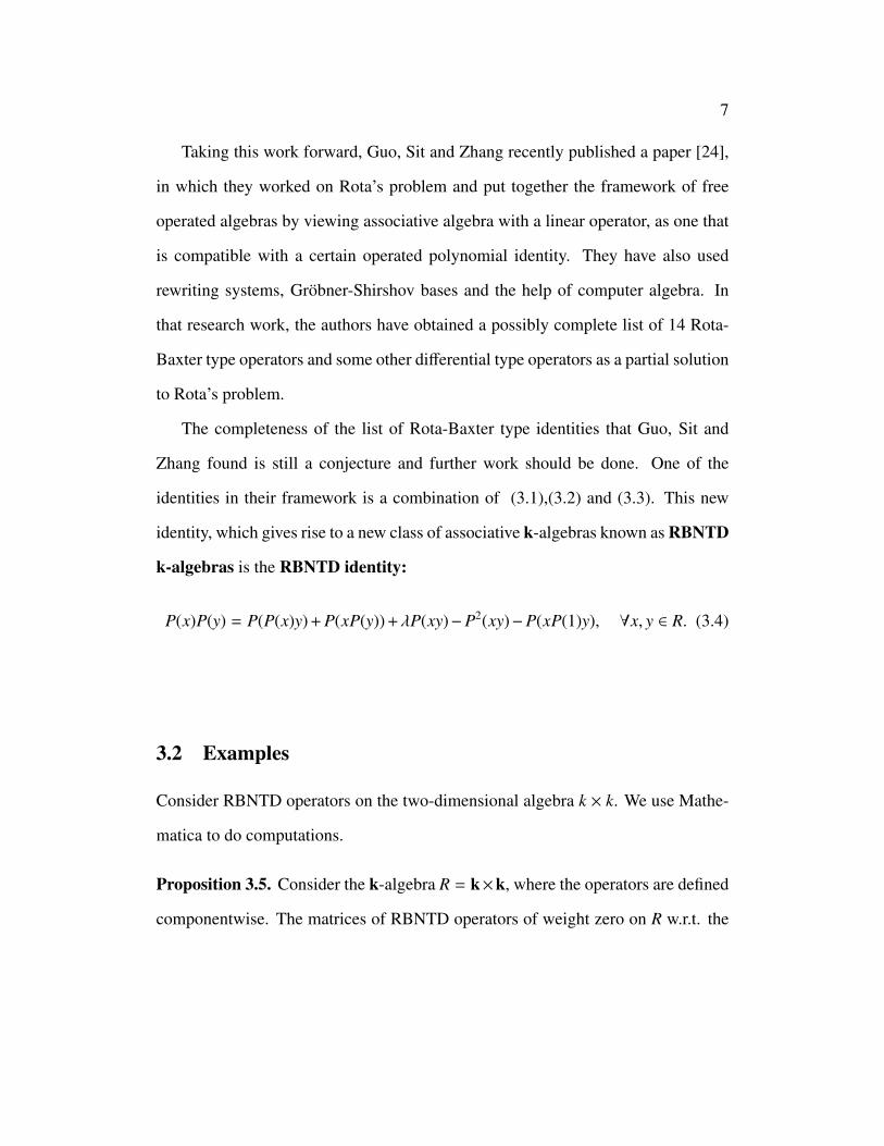
Proposition 3.5. Consider the k-algebra R = k×k, where the operators are defined

componentwise. The matrices of RBNTD operators of weight zero on R w.r.t. the

8

basis e1 = (1, 0) and e2 = (0, 1) is

M =

0 0

c −c

, c ∈ k

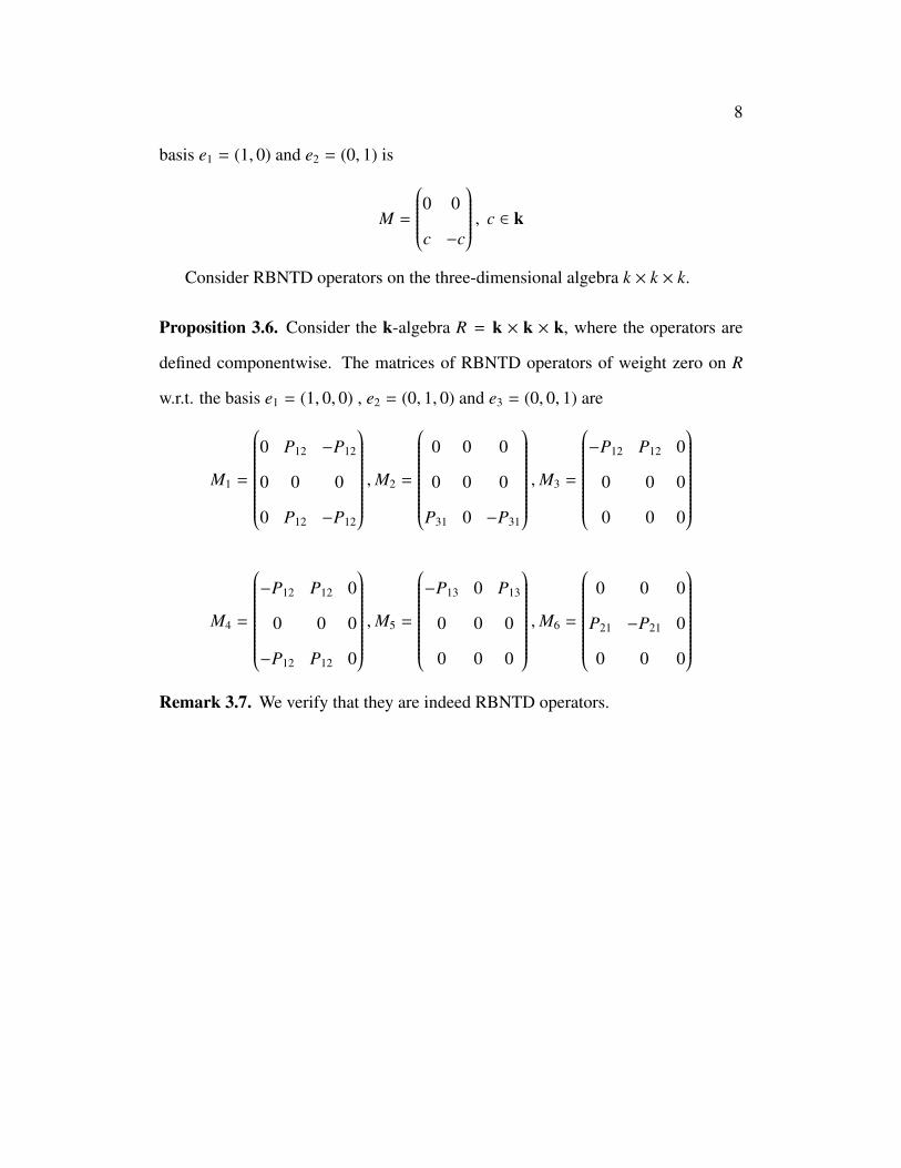
Consider RBNTD operators on the three-dimensional algebra k × k × k.

Proposition 3.6. Consider the k-algebra R = k × k × k, where the operators are

defined componentwise. The matrices of RBNTD operators of weight zero on R

w.r.t. the basis e1 = (1, 0, 0) , e2 = (0, 1, 0) and e3 = (0, 0, 1) are

M1 =

0 P12 −P12

0 0 0

0 P12 −P12

,M2 =

0 0 0

0 0 0

P31 0 −P31

,M3 =

−P12 P12 0

0 0 0

0 0 0

M4 =

−P12 P12 0

0 0 0

−P12 P12 0

,M5 =

−P13 0 P13

0 0 0

0 0 0

,M6 =

0 0 0

P21 −P21 0

0 0 0

Remark 3.7. We verify that they are indeed RBNTD operators.

9

4 Free Commutative RBNTD algebras and

shuffle products

The shuffle product is an important concept in algebra, combinatorics and topology.

Several generalizations that have been found in recent years that are applied to

algebra, combinatorics and number theory.

4.1 The shuffle product

The shuffle product can be defined in two ways, namely recursively or explicitly.

Let V be a k-module. Consider the k-module

T (V) :=⊕n≥0

V⊗n = k ⊕ V ⊕ V⊗2 ⊕ · · · .

Here the tensor products are taken over k and we take V⊗0 = k.

Let two pure tensors a = a1 ⊗ · · · ⊗ am ∈ V⊗m and b = b1 ⊗ · · · ⊗ bn ∈ V⊗n be

given. To describe the shuffle product of the two tensors, think of them as two decks

of cards. A shuffle of a and b is just a shuffle of the two decks of cards — a tensor

list from the factors of a and b in which the natural orders of the ai’s and b j’s are

preserved. To form the shuffle product of a and b, one sums together all possible

shuffles of the two pure tensors.

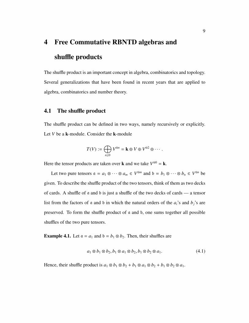
Example 4.1. Let a = a1 and b = b1 ⊗ b2. Then, their shuffles are

a1 ⊗ b1 ⊗ b2, b1 ⊗ a1 ⊗ b2, b1 ⊗ b2 ⊗ a1. (4.1)

Hence, their shuffle product is a1 ⊗ b1 ⊗ b2 + b1 ⊗ a1 ⊗ b2 + b1 ⊗ b2 ⊗ a1.

10

Recall that the vector space T (V) is naturally equipped with a grading, where

|u | =n for u ∈ V⊗n. The shuffle product on T (V) starts with the shuffles of permuta-

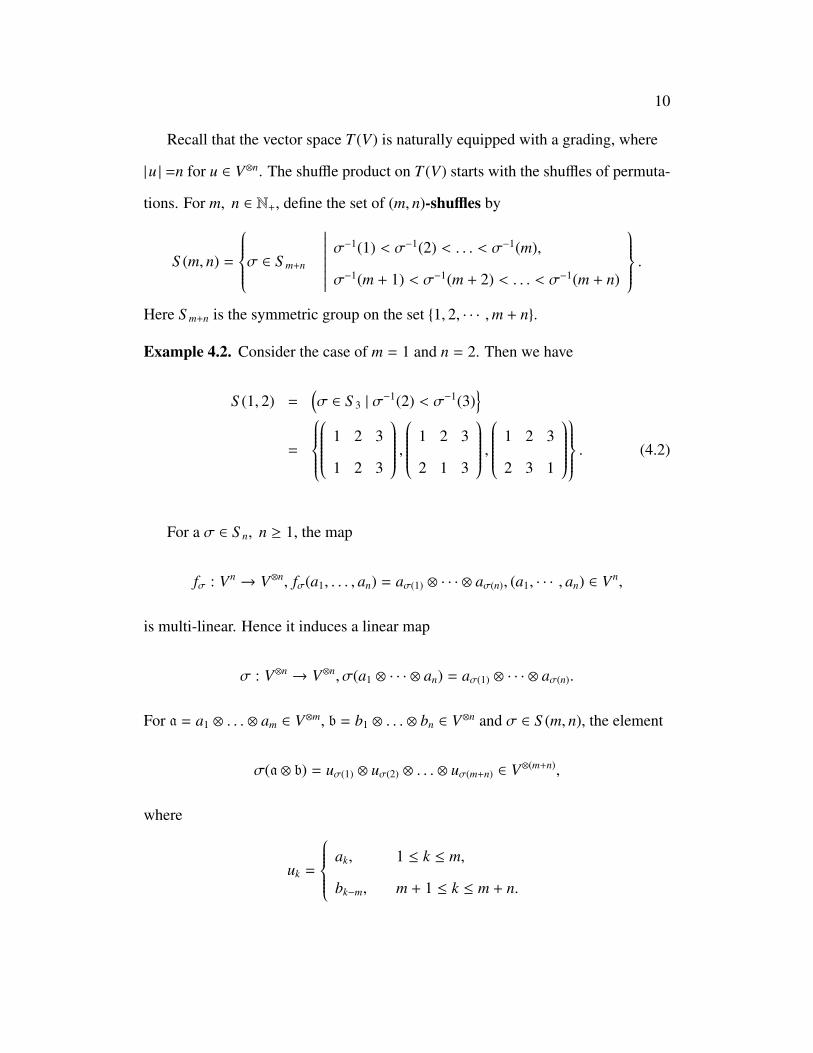
tions. For m, n ∈ N+, define the set of (m, n)-shuffles by

S (m, n) =

σ ∈ S m+n

∣∣∣∣∣∣∣∣∣σ−1(1) < σ−1(2) < . . . < σ−1(m),

σ−1(m + 1) < σ−1(m + 2) < . . . < σ−1(m + n)

.Here S m+n is the symmetric group on the set {1, 2, · · · ,m + n}.

Example 4.2. Consider the case of m = 1 and n = 2. Then we have

S (1, 2) =(σ ∈ S 3 | σ

−1(2) < σ−1(3)}

=

1 2 3

1 2 3

, 1 2 3

2 1 3

, 1 2 3

2 3 1

. (4.2)

For a σ ∈ S n, n ≥ 1, the map

fσ : Vn → V⊗n, fσ(a1, . . . , an) = aσ(1) ⊗ · · · ⊗ aσ(n), (a1, · · · , an) ∈ Vn,

is multi-linear. Hence it induces a linear map

σ : V⊗n → V⊗n, σ(a1 ⊗ · · · ⊗ an) = aσ(1) ⊗ · · · ⊗ aσ(n).

For a = a1 ⊗ . . . ⊗ am ∈ V⊗m, b = b1 ⊗ . . . ⊗ bn ∈ V⊗n and σ ∈ S (m, n), the element

σ(a ⊗ b) = uσ(1) ⊗ uσ(2) ⊗ . . . ⊗ uσ(m+n) ∈ V⊗(m+n),

where

uk =

ak, 1 ≤ k ≤ m,

bk−m, m + 1 ≤ k ≤ m + n.

11

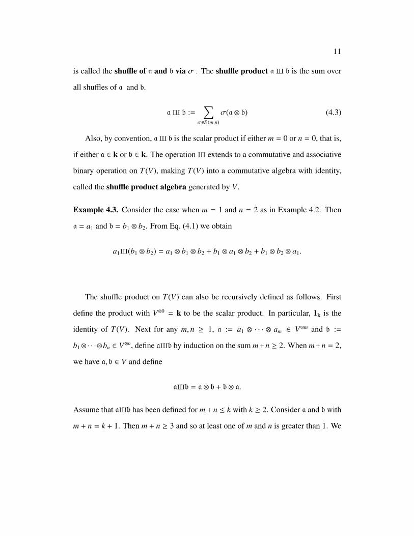
is called the shuffle of a and b via σ . The shuffle product aX b is the sum over

all shuffles of a and b.

aX b :=∑

σ∈S (m,n)

σ(a ⊗ b) (4.3)

Also, by convention, aX b is the scalar product if either m = 0 or n = 0, that is,

if either a ∈ k or b ∈ k. The operation X extends to a commutative and associative

binary operation on T (V), making T (V) into a commutative algebra with identity,

called the shuffle product algebra generated by V .

Example 4.3. Consider the case when m = 1 and n = 2 as in Example 4.2. Then

a = a1 and b = b1 ⊗ b2. From Eq. (4.1) we obtain

a1X(b1 ⊗ b2) = a1 ⊗ b1 ⊗ b2 + b1 ⊗ a1 ⊗ b2 + b1 ⊗ b2 ⊗ a1.

The shuffle product on T (V) can also be recursively defined as follows. First

define the product with V⊗0 = k to be the scalar product. In particular, 1k is the

identity of T (V). Next for any m, n ≥ 1, a := a1 ⊗ · · · ⊗ am ∈ V⊗m and b :=

b1⊗· · ·⊗bn ∈ V⊗n, define aXb by induction on the sum m+n ≥ 2. When m+n = 2,

we have a, b ∈ V and define

aXb = a ⊗ b + b ⊗ a.

Assume that aXb has been defined for m + n ≤ k with k ≥ 2. Consider a and b with

m + n = k + 1. Then m + n ≥ 3 and so at least one of m and n is greater than 1. We

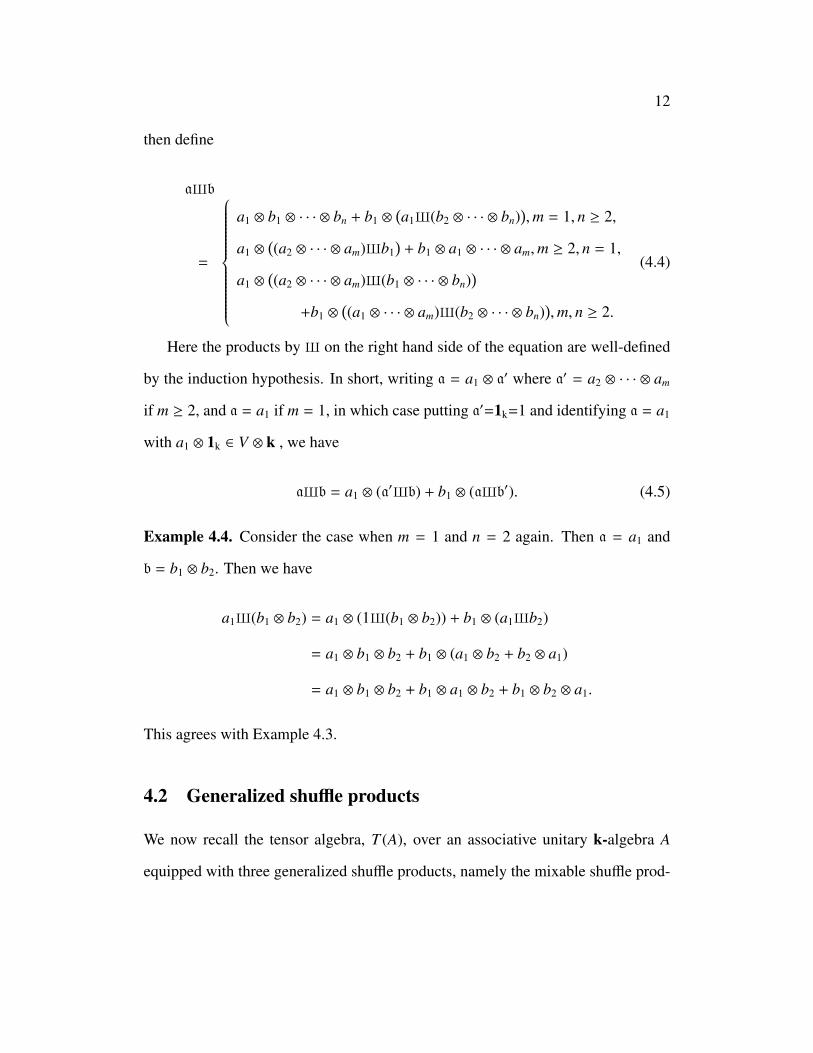
12

then define

aXb

=

a1 ⊗ b1 ⊗ · · · ⊗ bn + b1 ⊗(a1X(b2 ⊗ · · · ⊗ bn)

),m = 1, n ≥ 2,

a1 ⊗((a2 ⊗ · · · ⊗ am)Xb1

)+ b1 ⊗ a1 ⊗ · · · ⊗ am,m ≥ 2, n = 1,

a1 ⊗((a2 ⊗ · · · ⊗ am)X(b1 ⊗ · · · ⊗ bn)

)+b1 ⊗

((a1 ⊗ · · · ⊗ am)X(b2 ⊗ · · · ⊗ bn)

),m, n ≥ 2.

(4.4)

Here the products by X on the right hand side of the equation are well-defined

by the induction hypothesis. In short, writing a = a1 ⊗ a′ where a′ = a2 ⊗ · · · ⊗ am

if m ≥ 2, and a = a1 if m = 1, in which case putting a′=1k=1 and identifying a = a1

with a1 ⊗ 1k ∈ V ⊗ k , we have

aXb = a1 ⊗ (a′Xb) + b1 ⊗ (aXb′). (4.5)

Example 4.4. Consider the case when m = 1 and n = 2 again. Then a = a1 and

b = b1 ⊗ b2. Then we have

a1X(b1 ⊗ b2) = a1 ⊗ (1X(b1 ⊗ b2)) + b1 ⊗ (a1Xb2)

= a1 ⊗ b1 ⊗ b2 + b1 ⊗ (a1 ⊗ b2 + b2 ⊗ a1)

= a1 ⊗ b1 ⊗ b2 + b1 ⊗ a1 ⊗ b2 + b1 ⊗ b2 ⊗ a1.

This agrees with Example 4.3.

4.2 Generalized shuffle products

We now recall the tensor algebra, T (A), over an associative unitary k-algebra A

equipped with three generalized shuffle products, namely the mixable shuffle prod-

13

uct defined in [22] and the left and right shuffle product defined in [16]. First, we

will give explicit formulae for these products and then their recursive definitions.

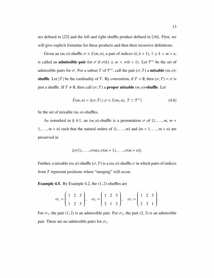
Given an (m, n)-shuffle σ ∈ S (m, n), a pair of indices (k, k + 1), 1 ≤ k < m + n,

is called an admissible pair for σ if σ(k) ≤ m < σ(k + 1). Let T σ be the set of

admissible pairs for σ. For a subset T of T σ, call the pair (σ,T ) a mixable (m, n)-

shuffle. Let |T | be the cardinality of T . By convention, if T = ∅, then (σ,T ) = σ is

just a shuffle. If T , ∅, then call (σ; T ) a proper mixable (m, n)-shuffle. Let

S (m, n) = {(σ,T ) | σ ∈ S (m, n), T ⊂ T σ} (4.6)

be the set of mixable (m, n)-shuffles.

As remarked in § 4.1, an (m, n)-shuffle is a permutation σ of {1, . . . ,m, m +

1, . . . ,m + n} such that the natural orders of {1, . . . ,m} and {m + 1, . . . ,m + n} are

preserved in

{σ(1), . . . , σ(m), σ(m + 1), . . . , σ(m + n)}.

Further, a mixable (m, n)-shuffle (σ,T ) is a (m, n)-shuffle σ in which pairs of indices

from T represent positions where “merging” will occur.

Example 4.5. By Example 4.2, the (1, 2)-shuffles are

σ1 =

1 2 3

1 2 3

, σ2 =

1 2 3

2 1 3

, σ3 =

1 2 3

2 3 1

.For σ1, the pair (1, 2) is an admissible pair. For σ2, the pair (2, 3) is an admissible

pair. There are no admissible pairs for σ3.

14

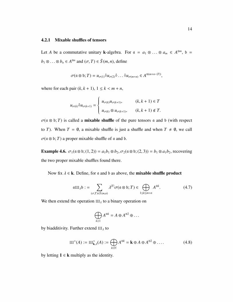
4.2.1 Mixable shuffles of tensors

Let A be a commutative unitary k-algebra. For a = a1 ⊗ . . . ⊗ am ∈ A⊗m, b =

b1 ⊗ . . . ⊗ bn ∈ A⊗n and (σ,T ) ∈ S (m, n), define

σ(a ⊗ b; T ) = uσ(1)�uσ(2)� . . . �uσ(m+n) ∈ A⊗(m+n−|T |),

where for each pair (k, k + 1), 1 ≤ k < m + n,

uσ(k)�uσ(k+1) =

uσ(k)uσ(k+1), (k, k + 1) ∈ T

uσ(k) ⊗ uσ(k+1), (k, k + 1) < T.

σ(a ⊗ b; T ) is called a mixable shuffle of the pure tensors a and b (with respect

to T ). When T = ∅, a mixable shuffle is just a shuffle and when T , ∅, we call

σ(a ⊗ b; T ) a proper mixable shuffle of a and b.

Example 4.6. σ1(a ⊗ b; (1, 2)) = a1b1 ⊗ b2, σ2(a ⊗ b; (2, 3)) = b1 ⊗ a1b2, recovering

the two proper mixable shuffles found there.

Now fix λ ∈ k. Define, for a and b as above, the mixable shuffle product

aXλb : =∑

(σ,T )∈S (m,n)

λ|T |σ(a ⊗ b; T ) ∈⊕

1≤k≤m+n

A⊗k. (4.7)

We then extend the operation Xλ to a binary operation on

⊕k≥1

A⊗k = A ⊕ A⊗2 ⊕ . . .

by biadditivity. Further extend Xλ to

X+(A) := X+k,λ(A) :=

⊕k∈N

A⊗k = k ⊕ A ⊕ A⊗2 ⊕ . . . . (4.8)

by letting 1 ∈ k multiply as the identity.

15

Example 4.7. Continuing with Example 4.6, we have

a1Xλ(b1 ⊗ b2) (4.9)

= a1 ⊗ b1 ⊗ b2 + b1 ⊗ a1 ⊗ b2 + b1 ⊗ b2 ⊗ a1 (improper mixable shuffles)

+ λa1b1 ⊗ b2 + λb1 ⊗ a1b2 (proper mixable shuffles).

Theorem 4.8. [22] The k-module X+(A) with the mixable shuffle product Xλ

is a commutative unitary k-algebra. Further, the tensor product algebra X(A) :=

A ⊗X+(A) with the linear operator

PA : X(A)→X(A); PA(a) = 1A ⊗ a,

is the free commutative Rota-Baxter algebra on A.

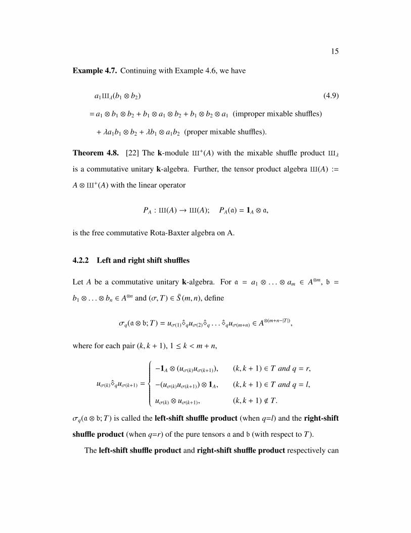
4.2.2 Left and right shift shuffles

Let A be a commutative unitary k-algebra. For a = a1 ⊗ . . . ⊗ am ∈ A⊗m, b =

b1 ⊗ . . . ⊗ bn ∈ A⊗n and (σ,T ) ∈ S (m, n), define

σq(a ⊗ b; T ) = uσ(1)�quσ(2)�q . . . �quσ(m+n) ∈ A⊗(m+n−|T |),

where for each pair (k, k + 1), 1 ≤ k < m + n,

uσ(k)�quσ(k+1) =

−1A ⊗ (uσ(k)uσ(k+1)), (k, k + 1) ∈ T and q = r,

−(uσ(k)uσ(k+1)) ⊗ 1A, (k, k + 1) ∈ T and q = l,

uσ(k) ⊗ uσ(k+1), (k, k + 1) < T.

σq(a ⊗ b; T ) is called the left-shift shuffle product (when q=l) and the right-shift

shuffle product (when q=r) of the pure tensors a and b (with respect to T ).

The left-shift shuffle product and right-shift shuffle product respectively can

16

also be defined with the convention x⊗1k=x, by

a�lb = a1 ⊗ (a′�lb) + b1 ⊗ (a�lb′) − a1b1 ⊗ 1A ⊗ (a′�lb

′)

a�rb = a1 ⊗ (a′�rb) + b1 ⊗ (a�rb′) − 1A ⊗ a1b1 ⊗ (a′�rb

′)

where a=a1 ⊗ a′ and b=b1 ⊗ b

′ as before.

Example 4.9. We have

a1�l(b1 ⊗ b2)

= a1 ⊗ b1 ⊗ b2 + b1 ⊗ a1 ⊗ b2 + b1 ⊗ b2 ⊗ a1 (shuffles) (4.10)

− (a1b1) ⊗ 1A ⊗ b2 − b1 ⊗ (a1b2) ⊗ 1A (left-shift shuffles).

and

a1�r(b1 ⊗ b2)

= a1 ⊗ b1 ⊗ b2 + b1 ⊗ a1 ⊗ b2 + b1 ⊗ b2 ⊗ a1 (shuffles) (4.11)

− 1A ⊗ (a1b1) ⊗ b2 − b1 ⊗ 1A ⊗ (a1b2) (right-shift shuffles).

Theorem 4.10. [16] The k-module X+(A) with the right-shift (resp. left-shift)

shuffle product �r (resp.�l) is a commutative unitary k-algebra. Further, the tensor

product algebra→

X (A) := A ⊗X+(A) (resp.←

X (A) := A ⊗X+(A)) with the linear

operators

PA :→

X (A)→→

X (A); PA(a) = 1A ⊗ a,

QA :←

X (A)→←

X (A)); QA(a) = a ⊗ 1A,

is the free commutative Nijenhuis (resp. TD ) algebra on A.

17

4.3 RBNTD shuffle product

Now, let us define our new RBNTD-shuffle product, denoted by ~λ, on

X+(A) := X+k,λ(A) :=

⊕k∈N

A⊗k = k ⊕ A ⊕ A⊗2 ⊕ · · ·

For this, we only need to define the product of two pure tensors and then to

extend by bilinearity. Any tensor a in A⊗k is said to have length k, denoted by | a |.

For two pure tensors a = a1 ⊗ . . . ⊗ am ∈ A⊗m and b = b1 ⊗ . . . ⊗ bn ∈ A⊗n, we

define a ~λ b by induction on m + n. If m = n = 0, then a, b ∈ k and we just define

a~λb = ab ∈ k. Assume the product has been defined for a, b with m+n ≤ k, and let

a, b be pure tensors with m + n = k + 1. If either m or n is zero, then we define a~λ b

by the scalar product. If neither m nor n is zero, then we have a = a1⊗a′, b = b1⊗b

′

with a1, b1 ∈ A and a′ ∈ A⊗(m−1) and b′ ∈ A⊗(n−1). We then define

a ~λ b = a1 ⊗ (a′ ~λ b) + b1 ⊗ (a ~λ b′) + λ(a1b1) ⊗ (a′ ~λ b′)

− 1A ⊗ (a1b1) ⊗ (a′ ~λ b′) − a1b1 ⊗ ((a′ ~λ 1A) ~λ b′) (4.12)

Here the terms on the right hand side are well-defined by the induction hypothesis,

and a1b1 is the product in A.

Before we do any further computations, we need another result.

Lemma 4.11. For |a |>0, 1A ~λ a = λa = a ~λ 1A, where |a |=length of a.

Proof. We will divide the proof into two cases:

Case I: |a |=1. Then,

1A ~λ a = 1A ⊗ a + a ⊗ 1A + λa − 1A ⊗ a − a ⊗ ((1k ~λ 1A) ~λ 1k) = λa.

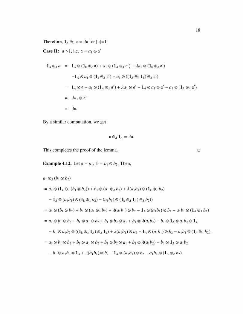
18

Therefore, 1A ~λ a = λa for |a |=1.

Case II: |a |>1, i.e. a = a1 ⊗ a′

1A ~λ a = 1A ⊗ (1k ~λ a) + a1 ⊗ (1A ~λ a′) + λa1 ⊗ (1k ~λ a

′)

−1A ⊗ a1 ⊗ (1k ~λ a′) − a1 ⊗ ((1A ~λ 1k) ~λ a′)

= 1A ⊗ a + a1 ⊗ (1A ~λ a′) + λa1 ⊗ a

′ − 1A ⊗ a1 ⊗ a′ − a1 ⊗ (1A ~λ a

′)

= λa1 ⊗ a′

= λa.

By a similar computation, we get

a ~λ 1A = λa.

This completes the proof of the lemma. �

Example 4.12. Let a = a1, b = b1 ⊗ b2. Then,

a1 ~λ (b1 ⊗ b2)

= a1 ⊗ (1k ~λ (b1 ⊗ b2)) + b1 ⊗ (a1 ~λ b2) + λ(a1b1) ⊗ (1k ~λ b2)

− 1A ⊗ (a1b1) ⊗ (1k ~λ b2) − (a1b1) ⊗ (1k ~λ 1A) ~λ b2))

= a1 ⊗ (b1 ⊗ b2) + b1 ⊗ (a1 ~λ b2) + λ(a1b1) ⊗ b2 − 1A ⊗ (a1b1) ⊗ b2 − a1b1 ⊗ (1A ~λ b2)

= a1 ⊗ b1 ⊗ b2 + b1 ⊗ a1 ⊗ b2 + b1 ⊗ b2 ⊗ a1 + b1 ⊗ λ(a1b2) − b1 ⊗ 1A ⊗ a1b2 ⊗ 1k

− b1 ⊗ a1b2 ⊗ ((1k ~λ 1A) ~λ 1k) + λ(a1b1) ⊗ b2 − 1A ⊗ (a1b1) ⊗ b2 − a1b1 ⊗ (1A ~λ b2).

= a1 ⊗ b1 ⊗ b2 + b1 ⊗ a1 ⊗ b2 + b1 ⊗ b2 ⊗ a1 + b1 ⊗ λ(a1b2) − b1 ⊗ 1A ⊗ a1b2

− b1 ⊗ a1b2 ⊗ 1A + λ(a1b1) ⊗ b2 − 1A ⊗ (a1b1) ⊗ b2 − a1b1 ⊗ (1A ~λ b2).

19

By applying above lemma, we will get

a1 ~λ (b1 ⊗ b2)


− b1 ⊗ a1b2 ⊗ 1A + λ(a1b1) ⊗ b2 − 1A ⊗ (a1b1) ⊗ b2 − a1b1 ⊗ (λb2)


− b1 ⊗ a1b2 ⊗ 1A − 1A ⊗ (a1b1) ⊗ b2.

Now, we prove the associativity of the RBNTD shuffle product.

Theorem 4.13. The RBNTD shuffle product is associative. i.e.

(a ~λ b) ~λ c = a ~λ (b ~λ c).

Proof. We will prove the associativity in five cases:

Case I:If |a |= 0, |b |= 0, | c |= 0, then all are scalars and the associativity holds.

Case II:If one of |a |, |b |= 0, | c | arbitrary, then also the associativity holds.

Case III:If |a |= 1, |b |= 1, | c |= 1, then to check

(a ~λ b) ~λ c = a ~λ (b ~λ c).

We will start with computing the left hand side which is:

(a ~λ b) ~λ c = (a ⊗ b + b ⊗ a + λab − 1A ⊗ ab − ab ⊗ 1A) ~λ c

= (a ⊗ b) ~λ c + (b ⊗ a) ~λ c + (λab) ~λ c

−(1A ⊗ ab) ~λ c − (ab ⊗ 1A) ~λ c.

Expanding further each term:

(a ~λ b) ~λ c = a ⊗ (b ~λ c) + c ⊗ (a ⊗ b) + λac ⊗ b − 1A ⊗ ac ⊗ b

20

−ac ⊗ (b ~λ 1A) + b ⊗ (a ~λ c) + c ⊗ (b ⊗ a) + λbc ⊗ a

−1A ⊗ bc ⊗ a − bc ⊗ (a ~λ 1A) + λab ⊗ c + c ⊗ λab

+λ2abc − 1A ⊗ λabc − λabc ⊗ 1A − 1A ⊗ (ab ~λ c)

−c ⊗ (1A ⊗ ab) − λc ⊗ ab + 1A ⊗ c ⊗ ab + c ⊗ (ab ~λ 1A)

−ab ⊗ (1A ~λ c) − c ⊗ (ab ⊗ 1A) − λabc ⊗ 1A

+1A ⊗ abc ⊗ 1A + abc ⊗ (1A ~λ 1A).

Further expanding ~λ product, we get:

(a ~λ b) ~λ c = a ⊗ (b ⊗ c) + a ⊗ (c ⊗ b) + a ⊗ λbc − a ⊗ (1A ⊗ bc)

−a ⊗ (bc ⊗ 1A) + c ⊗ (a ⊗ b) + λac ⊗ b − 1A ⊗ ac ⊗ b

−ac ⊗ λb + b ⊗ (a ⊗ c) + b ⊗ (c ⊗ a) + b ⊗ λac

−b ⊗ λac − b ⊗ (1A ⊗ ac) + c ⊗ (b ⊗ a) + λbc ⊗ a

−1A ⊗ bc ⊗ a − bc ⊗ (a ~λ 1A) + λab ⊗ c + c ⊗ λab

+λ2abc − 1A ⊗ λabc − λabc ⊗ 1A − 1A ⊗ (ab ⊗ c)

−1A ⊗ (c ⊗ ab) − 1A ⊗ λabc + 1A ⊗ 1A ⊗ abc + 1A ⊗ abc ⊗ 1A

−c ⊗ (1A ⊗ ab) − λc ⊗ ab + 1A ⊗ c ⊗ ab + c ⊗ λ(ab)

−ab ⊗ (λc) − c ⊗ (ab ⊗ 1A) − λabc ⊗ 1A

+1A ⊗ abc ⊗ 1A + abc ⊗ (λ1A).

Simplifying:

(a ~λ b) ~λ c = a ⊗ (b ⊗ c)︸︷︷︸L1

+ a ⊗ (c ⊗ b)︸︷︷︸L2

+ a ⊗ λbc︸︷︷︸L3

− a ⊗ (1A ⊗ bc)︸︷︷︸L4

− a ⊗ (bc ⊗ 1A)︸︷︷︸L5

+ c ⊗ (a ⊗ b)︸︷︷︸L6

− 1A ⊗ ac ⊗ b︸︷︷︸L7

+ b ⊗ (a ⊗ c)︸︷︷︸L8

21

+ b ⊗ (c ⊗ a)︸︷︷︸L9

+ b ⊗ λac︸︷︷︸L10

− b ⊗ (1A ⊗ ac)︸︷︷︸L11

− b ⊗ (ac ⊗ 1A)︸︷︷︸L12

+ c ⊗ (b ⊗ a)︸︷︷︸L13

− 1A ⊗ bc ⊗ a︸︷︷︸L14

+ c ⊗ λab︸︷︷︸L15

+ λ2abc︸︷︷︸

L16

− 1A ⊗ λabc︸︷︷︸L17

− 1A ⊗ (ab ⊗ c)︸︷︷︸L18

− 1A ⊗ λabc︸︷︷︸L19

+ 1A ⊗ 1A ⊗ abc︸︷︷︸L20

+ 1A ⊗ abc ⊗ 1A︸︷︷︸L21

− c ⊗ (1A ⊗ ab)︸︷︷︸L22

− c ⊗ (ab ⊗ 1A)︸︷︷︸L23

− λabc ⊗ 1A︸︷︷︸L24

+ 1A ⊗ abc ⊗ 1A︸︷︷︸L25

.

Now, computing the right hand side which is a ~λ (b ~λ c).

a ~λ (b ~λ c) = a ~λ (b ⊗ c + c ⊗ b + λbc − 1A ⊗ bc − bc ⊗ 1A)

= a ~λ (b ⊗ c) + a ~λ (c ⊗ b) + a ~λ (λbc)

−a ~λ (1A ⊗ bc) − a ~λ (bc ⊗ 1A).

By a similar computation as for the left hand side, we get

a ~λ (b ~λ c) = a ⊗ (b ⊗ c)︸︷︷︸R1

+ b ⊗ (a ⊗ c)︸︷︷︸R2

+ b ⊗ (c ⊗ a)︸︷︷︸R3

+ b ⊗ (λac)︸︷︷︸R4

− b ⊗ 1A ⊗ ac︸︷︷︸R5

− b ⊗ ac ⊗ 1A︸︷︷︸R6

− 1A ⊗ ab ⊗ c︸︷︷︸R7

+ a ⊗ (c ⊗ b)︸︷︷︸R8

+ c ⊗ (a ⊗ b)︸︷︷︸R9

+ c ⊗ (b ⊗ a)︸︷︷︸R10

+ c ⊗ λab︸︷︷︸R11

− c ⊗ 1A ⊗ ab︸︷︷︸R12

− c ⊗ ab ⊗ 1A︸︷︷︸R13

− 1A ⊗ ac ⊗ b︸︷︷︸R14

+ a ⊗ λbc︸︷︷︸R15

+ λ2abc︸︷︷︸

R16

− 1A ⊗ λabc︸︷︷︸R17

− λabc ⊗ 1A︸︷︷︸R18

− a ⊗ λbc︸︷︷︸R19

− 1A ⊗ (bc ⊗ a)︸︷︷︸R20

− 1A ⊗ λabc︸︷︷︸R21

+ 1A ⊗ 1A ⊗ abc︸︷︷︸R22

+ 1A ⊗ abc ⊗ 1A︸︷︷︸R23

− a ⊗ (bc ⊗ 1A)︸︷︷︸R24

+ 1A ⊗ abc ⊗ 1A︸︷︷︸R25

.

For 1 ≤ i ≤ 25, let Li (resp Ri) be the ith term in the left hand side (resp. in the right

22

hand side ). Then by the induction hypothesis, Li = Rσ(i). Here the permutation

σ ∈ Σ25 is given by

σ =

1 2 3 4 5 6 7 8 9 10 11 12 13

1 8 15 19 24 9 14 2 3 4 5 6 10

14 15 16 17 18 19 20 21 22 23 24 25

20 11 16 17 7 21 22 25 12 13 18 23

.Case IV: If |a |= 1, |b |= 1, | c |> 1, then similar to above case.

Case V: If | a |≥ 2, | b |≥ 2 and | c | arbitrary. Then, let a = a1 ⊗ a′, b = b1 ⊗ b

′ and

c = c1 ⊗ c′.

We will prove this result using induction on |a | + |b | + | c |.

If |a |= 0, |b |= 0, | c |= 0, holds by Case I.

Assume that the associativity holds for |a | + |b | + | c |≤ k.

To check for |a | + |b | + | c |=k+1.

Now, first we will work on the left hand side (a ~λ b) ~λ c.

(a ~λ b) ~λ c =[a1 ⊗ (a′ ~λ b) + b1 ⊗ (a ~λ b′) + λa1b1 ⊗ (a′ ~λ b′)

−1A ⊗ a1b1 ⊗ (a′ ~λ b′) − a1b1 ⊗ ((a′ ~λ 1A) ~λ b′)]~λ c.

Since |a′ |≥ 1(|a |≥ 2), apply Lemma 4.11 on the last term,

(a ~λ b) ~λ c =[a1 ⊗ (a′ ~λ b) + b1 ⊗ (a ~λ b′) + λa1b1 ⊗ (a′ ~λ b′)

−1A ⊗ a1b1 ⊗ (a′ ~λ b′) − a1b1 ⊗ ((λa′ ~λ b′)]~λ c.

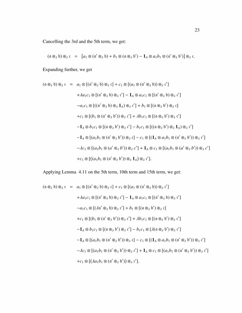
23

Cancelling the 3rd and the 5th term, we get:

(a ~λ b) ~λ c =[a1 ⊗ (a′ ~λ b) + b1 ⊗ (a ~λ b′) − 1A ⊗ a1b1 ⊗ (a′ ~λ b′)

]~λ c.

Expanding further, we get

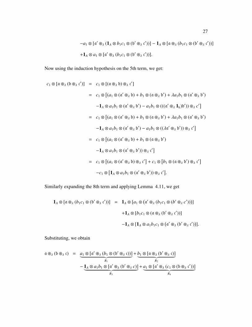
(a ~λ b) ~λ c = a1 ⊗ [(a′ ~λ b) ~λ c] + c1 ⊗ [(a1 ⊗ (a′ ~λ b)) ~λ c′]

+λa1c1 ⊗ [(a′ ~λ b) ~λ c′] − 1A ⊗ a1c1 ⊗ [(a′ ~λ b) ~λ c′]

−a1c1 ⊗ [((a′ ~λ b) ~λ 1A) ~λ c′] + b1 ⊗ [(a ~λ b′) ~λ c]

+c1 ⊗ [(b1 ⊗ (a′ ~λ b′)) ~λ c′] + λb1c1 ⊗ [(a ~λ b′) ~λ c′]

−1A ⊗ b1c1 ⊗ [(a ~λ b′) ~λ c′] − b1c1 ⊗ [((a ~λ b′) ~λ 1A) ~λ c′]

−1A ⊗ [(a1b1 ⊗ (a′ ~λ b′)) ~λ c] − c1 ⊗ [(1A ⊗ a1b1 ⊗ (a′ ~λ b′)) ~λ c′]

−λc1 ⊗ [(a1b1 ⊗ (a′ ~λ b′)) ~λ c′] + 1A ⊗ c1 ⊗ [(a1b1 ⊗ (a′ ~λ b′)) ~λ c′]

+c1 ⊗ [((a1b1 ⊗ (a′ ~λ b′)) ~λ 1A

)~λ c

′].

Applying Lemma 4.11 on the 5th term, 10th term and 15th term, we get:


+λa1c1 ⊗ [(a′ ~λ b) ~λ c′] − 1A ⊗ a1c1 ⊗ [(a′ ~λ b) ~λ c′]

−a1c1 ⊗ [(λa′ ~λ b) ~λ c′] + b1 ⊗ [(a ~λ b′) ~λ c]

+c1 ⊗ [(b1 ⊗ (a′ ~λ b′)) ~λ c′] + λb1c1 ⊗ [(a ~λ b′) ~λ c′]

−1A ⊗ b1c1 ⊗ [(a ~λ b′) ~λ c′] − b1c1 ⊗ [λ(a ~λ b′) ~λ c′]


−λc1 ⊗ [(a1b1 ⊗ (a′ ~λ b′)) ~λ c′] + 1A ⊗ c1 ⊗ [(a1b1 ⊗ (a′ ~λ b′)) ~λ c′]

+c1 ⊗ [(λa1b1 ⊗ (a′ ~λ b′)

)~λ c

′].

24

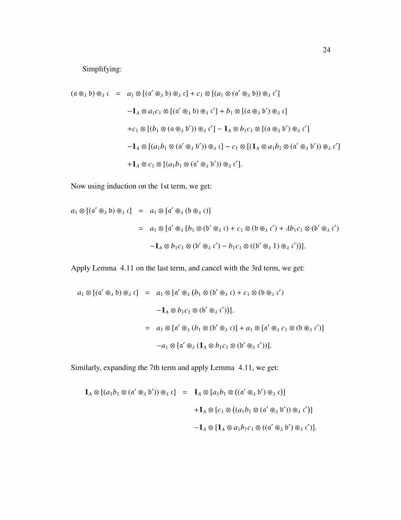
Simplifying:


−1A ⊗ a1c1 ⊗ [(a′ ~λ b) ~λ c′] + b1 ⊗ [(a ~λ b′) ~λ c]

+c1 ⊗ [(b1 ⊗ (a ~λ b′)) ~λ c′] − 1A ⊗ b1c1 ⊗ [(a ~λ b′) ~λ c′]


+1A ⊗ c1 ⊗ [(a1b1 ⊗ (a′ ~λ b′)) ~λ c′].

Now using induction on the 1st term, we get:

a1 ⊗ [(a′ ~λ b) ~λ c] = a1 ⊗ [a′ ~λ (b ~λ c)]

= a1 ⊗ [a′ ~λ(b1 ⊗ (b′ ~λ c) + c1 ⊗ (b ~λ c′) + λb1c1 ⊗ (b′ ~λ c′)

−1A ⊗ b1c1 ⊗ (b′ ~λ c′) − b1c1 ⊗ ((b′ ~λ 1) ~λ c′))].

Apply Lemma 4.11 on the last term, and cancel with the 3rd term, we get:

a1 ⊗ [(a′ ~λ b) ~λ c] = a1 ⊗ [a′ ~λ(b1 ⊗ (b′ ~λ c) + c1 ⊗ (b ~λ c′)

−1A ⊗ b1c1 ⊗ (b′ ~λ c′))].

= a1 ⊗ [a′ ~λ (b1 ⊗ (b′ ~λ c)] + a1 ⊗ [a′ ~λ c1 ⊗ (b ~λ c′)]

−a1 ⊗ [a′ ~λ (1A ⊗ b1c1 ⊗ (b′ ~λ c′))].

Similarly, expanding the 7th term and apply Lemma 4.11, we get:

1A ⊗ [(a1b1 ⊗ (a′ ~λ b′)) ~λ c] = 1A ⊗ [a1b1 ⊗((a′ ~λ b′) ~λ c

)]

+1A ⊗ [c1 ⊗((a1b1 ⊗ (a′ ~λ b′)) ~λ c′

)]

−1A ⊗ [1A ⊗ a1b1c1 ⊗ ((a′ ~λ b′) ~λ c′)].

25

Substituting, we will get:

(a ~λ b) ~λ c = a1 ⊗ [a′ ~λ (b1 ⊗ (b′ ~λ c)]︸︷︷︸L1

+ a1 ⊗ [a′ ~λ c1 ⊗ (b ~λ c′)]︸︷︷︸L2

− a1 ⊗ [a′ ~λ (1A ⊗ b1c1 ⊗ (b′ ~λ c′))]︸︷︷︸L3

+ c1 ⊗ [(a1 ⊗ (a′ ~λ b)) ~λ c′]︸︷︷︸L4

− 1A ⊗ a1c1 ⊗ [(a′ ~λ b) ~λ c′]︸︷︷︸L5

+ b1 ⊗ [(a ~λ b′) ~λ c]︸︷︷︸L6

+ c1 ⊗ [(b1 ⊗ (a ~λ b′)) ~λ c′]︸︷︷︸L7

− 1A ⊗ b1c1 ⊗ [(a ~λ b′) ~λ c′]︸︷︷︸L8

− 1A ⊗ [a1b1 ⊗((a′ ~λ b′) ~λ c

)]︸︷︷︸

L9

− 1A ⊗ [c1 ⊗((a1b1 ⊗ (a′ ~λ b′)) ~λ c′

)]︸︷︷︸

L10

+ 1A ⊗ [1A ⊗ a1b1c1 ⊗ ((a′ ~λ b′) ~λ c′)]︸︷︷︸L11

− c1 ⊗ [(1A ⊗ a1b1 ⊗ (a′ ~λ b′)) ~λ c′]︸︷︷︸L12

+ 1A ⊗ c1 ⊗ [(a1b1 ⊗ (a′ ~λ b′)) ~λ c′]︸︷︷︸L13

.

L10 and L13 will cancel each other, so we get:

(a ~λ b) ~λ c = a1 ⊗ [a′ ~λ (b1 ⊗ (b′ ~λ c)]︸︷︷︸L1

+ a1 ⊗ [a′ ~λ c1 ⊗ (b ~λ c′)]︸︷︷︸L2

− a1 ⊗ [a′ ~λ (1A ⊗ b1c1 ⊗ (b′ ~λ c′))]︸︷︷︸L3

+ c1 ⊗ [(a1 ⊗ (a′ ~λ b)) ~λ c′]︸︷︷︸L4

− 1A ⊗ a1c1 ⊗ [(a′ ~λ b) ~λ c′]︸︷︷︸L5

+ b1 ⊗ [(a ~λ b′) ~λ c]︸︷︷︸L6

+ c1 ⊗ [(b1 ⊗ (a ~λ b′)) ~λ c′]︸︷︷︸L7

− 1A ⊗ b1c1 ⊗ [(a ~λ b′) ~λ c′]︸︷︷︸L8

− 1A ⊗ [a1b1 ⊗((a′ ~λ b′) ~λ c

)]︸︷︷︸

L9

+ 1A ⊗ [1A ⊗ a1b1c1 ⊗ ((a′ ~λ b′) ~λ c′)]︸︷︷︸L10

− c1 ⊗ [(1A ⊗ a1b1 ⊗ (a′ ~λ b′)) ~λ c′]︸︷︷︸L11

.

Similarly, for the right hand side,

a ~λ (b ~λ c) = a ~λ [b1 ⊗ (b′ ~λ c) + c1 ⊗ (b ~λ c′) + λb1c1 ⊗ (b′ ~λ c′)

26

−1A ⊗ b1c1 ⊗ (b′ ~λ c′) − b1c1 ⊗((b′ ~λ 1k) ~λ c′

)].

Since |b′ |≥ 1(|b |≥ 2), apply Lemma 4.11 on the last term,

a ~λ (b ~λ c) = a ~λ [b1 ⊗ (b′ ~λ c) + c1 ⊗ (b ~λ c′) + λb1c1 ⊗ (b′ ~λ c′)

−1A ⊗ b1c1 ⊗ (b′ ~λ c′) − b1c1 ⊗ λ(b′ ~λ c′)].

Cancelling the 3rd and the 5th term, we get:

a ~λ (b ~λ c) = a ~λ [b1 ⊗ (b′ ~λ c) + c1 ⊗ (b ~λ c′) − 1A ⊗ b1c1 ⊗ (b′ ~λ c′)].

Expanding further,

a ~λ (b ~λ c) = a1 ⊗ [a′ ~λ (b1 ⊗ (b′ ~λ c))] + b1 ⊗ [a ~λ (b′ ~λ c)]

λa1b1 ⊗ [a′ ~λ (b′ ~λ c)] − 1A ⊗ a1b1 ⊗ [a′ ~λ (b′ ~λ c)]

a1b1 ⊗ [(a′ ~λ 1k) ~λ (b′ ~λ c)] + a1 ⊗ [a′ ~λ (c1 ⊗ (b ~λ c′))]

+c1 ⊗ [a ~λ (b ~λ c′)] + λa1c1 ⊗ [a′ ~λ (b ~λ c′)]

−1A ⊗ a1c1 ⊗ [a′ ~λ (b ~λ c′)] − a1c1 ⊗ [(a′ ~λ 1k) ~λ (b ~λ c′)]

−a1 ⊗ [a′ ~λ (1A ⊗ b1c1 ⊗ (b′ ~λ c′))] − 1A ⊗ [a ~λ (b1c1 ⊗ (b′ ~λ c′))]

−λa1 ⊗ [a′ ~λ (b1c1 ⊗ (b′ ~λ c′))] + 1A ⊗ a1 ⊗ [a′ ~λ (b1c1 ⊗ (b′ ~λ c′))]

−a1 ⊗ [(a′ ~λ 1k) ~λ (b1c1 ⊗ (b′ ~λ c′))].

Apply lemma 4.11 on the 5th, 10th and 15th term, and then simplify:

a ~λ (b ~λ c) = a1 ⊗ [a′ ~λ (b1 ⊗ (b′ ~λ c))] + b1 ⊗ [a ~λ (b′ ~λ c)]

−1A ⊗ a1b1 ⊗ [a′ ~λ (b′ ~λ c)] + a1 ⊗ [a′ ~λ (c1 ⊗ (b ~λ c′))]

+c1 ⊗ [a ~λ (b ~λ c′)] − 1A ⊗ a1c1 ⊗ [a′ ~λ (b ~λ c′)]

27

−a1 ⊗ [a′ ~λ (1A ⊗ b1c1 ⊗ (b′ ~λ c′))] − 1A ⊗ [a ~λ (b1c1 ⊗ (b′ ~λ c′))]

+1A ⊗ a1 ⊗ [a′ ~λ (b1c1 ⊗ (b′ ~λ c′))].

Now using the induction hypothesis on the 5th term, we get:

c1 ⊗ [a ~λ (b ~λ c′)] = c1 ⊗ [(a ~λ b) ~λ c′]

= c1 ⊗[(a1 ⊗ (a′ ~λ b) + b1 ⊗ (a ~λ b′) + λa1b1 ⊗ (a′ ~λ b′)

−1A ⊗ a1b1 ⊗ (a′ ~λ b′) − a1b1 ⊗ (((a′ ~λ 1k)b′)) ~λ c′]

= c1 ⊗[(a1 ⊗ (a′ ~λ b) + b1 ⊗ (a ~λ b′) + λa1b1 ⊗ (a′ ~λ b′)

−1A ⊗ a1b1 ⊗ (a′ ~λ b′) − a1b1 ⊗ ((λa′ ~λ b′)) ~λ c′]

= c1 ⊗[(a1 ⊗ (a′ ~λ b) + b1 ⊗ (a ~λ b′)

−1A ⊗ a1b1 ⊗ (a′ ~λ b′)) ~λ c′]

= c1 ⊗[(a1 ⊗ (a′ ~λ b) ~λ c′

]+ c1 ⊗

[b1 ⊗ (a ~λ b′) ~λ c′

]−c1 ⊗

[1A ⊗ a1b1 ⊗ (a′ ~λ b′)) ~λ c′

].

Similarly expanding the 8th term and applying Lemma 4.11, we get

1A ⊗ [a ~λ (b1c1 ⊗ (b′ ~λ c′))] = 1A ⊗ [a1 ⊗(a′ ~λ (b1c1 ⊗ (b′ ~λ c′))

)]

+1A ⊗ [b1c1 ⊗ (a ~λ (b′ ~λ c′))]

−1A ⊗ [1A ⊗ a1b1c1 ⊗(a′ ~λ (b′ ~λ c′)

)].

Substituting, we obtain

a ~λ (b ~λ c) = a1 ⊗ [a′ ~λ (b1 ⊗ (b′ ~λ c))]︸︷︷︸R1

+ b1 ⊗ [a ~λ (b′ ~λ c)]︸︷︷︸R2

− 1A ⊗ a1b1 ⊗ [a′ ~λ (b′ ~λ c)]︸︷︷︸R3

+ a1 ⊗ [a′ ~λ (c1 ⊗ (b ~λ c′))]︸︷︷︸R4

28

+ c1 ⊗[(a1 ⊗ (a′ ~λ b) ~λ c′

]︸︷︷︸R5

+ c1 ⊗[b1 ⊗ (a ~λ b′) ~λ c′

]︸︷︷︸R6

− c1 ⊗[1A ⊗ a1b1 ⊗ (a′ ~λ b′)) ~λ c′

]︸︷︷︸R7

− 1A ⊗ a1c1 ⊗ [a′ ~λ (b ~λ c′)]︸︷︷︸R8

− a1 ⊗ [a′ ~λ (1A ⊗ b1c1 ⊗ (b′ ~λ c′))]︸︷︷︸R9

− 1A ⊗ [a1 ⊗(a′ ~λ (b1c1 ⊗ (b′ ~λ c′))

)]︸︷︷︸

R10

− 1A ⊗ [b1c1 ⊗ (a ~λ (b′ ~λ c′))]︸︷︷︸R11

+ 1A ⊗ [1A ⊗ a1b1c1 ⊗(a′ ~λ (b′ ~λ c′)

)]︸︷︷︸

R12

+ 1A ⊗ a1 ⊗ [a′ ~λ (b1c1 ⊗ (b′ ~λ c′))]︸︷︷︸R13

.

R10 and R13 will cancel with each other. Hence, we have

a ~λ (b ~λ c) = a1 ⊗ [a′ ~λ (b1 ⊗ (b′ ~λ c))]︸︷︷︸R1

+ b1 ⊗ [a ~λ (b′ ~λ c)]︸︷︷︸R2

− 1A ⊗ a1b1 ⊗ [a′ ~λ (b′ ~λ c)]︸︷︷︸R3

+ a1 ⊗ [a′ ~λ (c1 ⊗ (b ~λ c′))]︸︷︷︸R4

+ c1 ⊗[(a1 ⊗ (a′ ~λ b)) ~λ c′

]︸︷︷︸R5

+ c1 ⊗[(b1 ⊗ (a ~λ b′)) ~λ c′

]︸︷︷︸R6

− c1 ⊗[1A ⊗ a1b1 ⊗ (a′ ~λ b′)) ~λ c′

]︸︷︷︸R7

− 1A ⊗ a1c1 ⊗ [a′ ~λ (b ~λ c′)]︸︷︷︸R8

− a1 ⊗ [a′ ~λ (1A ⊗ b1c1 ⊗ (b′ ~λ c′))]︸︷︷︸R9

− 1A ⊗ [b1c1 ⊗ (a ~λ (b′ ~λ c′))]︸︷︷︸R10

+ 1A ⊗ [1A ⊗ a1b1c1 ⊗(a′ ~λ (b′ ~λ c′)

)]︸︷︷︸

R11

.

For 1 ≤ i ≤ 11, let Li (resp Ri) be the ith term in the left hand side (resp. in the right

hand side ). Then by the induction hypothesis, Li = Rσ(i). Here the permutation

σ ∈ Σ11 is given by

σ =

1 2 3 4 5 6 7 8 9 10 11

1 4 9 5 8 2 6 10 3 11 7

Therefore, the associtivity is proved. �

29

Now, we also prove the commutativity of the RBNTD shuffle product.

Theorem 4.14. The RBNTD shuffle product ~λ is commutative. More precisely,

a ~λ b = b ~λ a.

Proof. For two pure tensors a and b, a := a1⊗· · ·⊗am ∈ A⊗m and b := b1⊗· · ·⊗bn ∈

A⊗n, let a = a1 ⊗ a′, a′ ∈ A⊗m−1 and b = b1 ⊗ b

′, b′ ∈ A⊗n−1. We will prove the result

by induction on m+n.

For m+n=0, a and b are scalars, so the result holds . Assume that the commuta-

tivity holds for m + n ≤ k. Now, we check for m+n=k+1.

a ~λ b = a1 ⊗ (a′ ~λ b) + b1 ⊗ (a ~λ b′) + λa1b1 ⊗ (a′ ~λ b′)

−1A ⊗ a1b1 ⊗ (a′ ~λ b′) − a1b1 ⊗ ((a′ ~λ 1A) ~λ b′).

For | a′ |, 0, we get a′ ~λ 1 = λa′ which gives us

a ~λ b = a1 ⊗ (a′ ~λ b) + b1 ⊗ (a ~λ b′)

−1A ⊗ a1b1 ⊗ (a′ ~λ b′).

Applying the induction hypothesis on all the terms because the sum of lengths ≤ k,

we get

a ~λ b = a1 ⊗ (b ~λ a′) + b1 ⊗ (b′ ~λ a)

−1A ⊗ a1b1 ⊗ (b′ ~λ a′).

Similarly, we compute b ~λ a.

b ~λ a = b1 ⊗ (b′ ~λ a) + a1 ⊗ (b ~λ a′) + λb1a1 ⊗ (b′ ~λ a′)

30

−1A ⊗ b1a1 ⊗ (b′ ~λ a′) − b1a1 ⊗ ((b′ ~λ 1A) ~λ a′).

For | b′ |, 0, we get b′ ~λ 1 = λb′, which gives us

b ~λ a = b1 ⊗ (b′ ~λ a) + a1 ⊗ (b ~λ a′)

−1A ⊗ b1a1 ⊗ (b′ ~λ a′).

So, they both agree since A is commutative. �

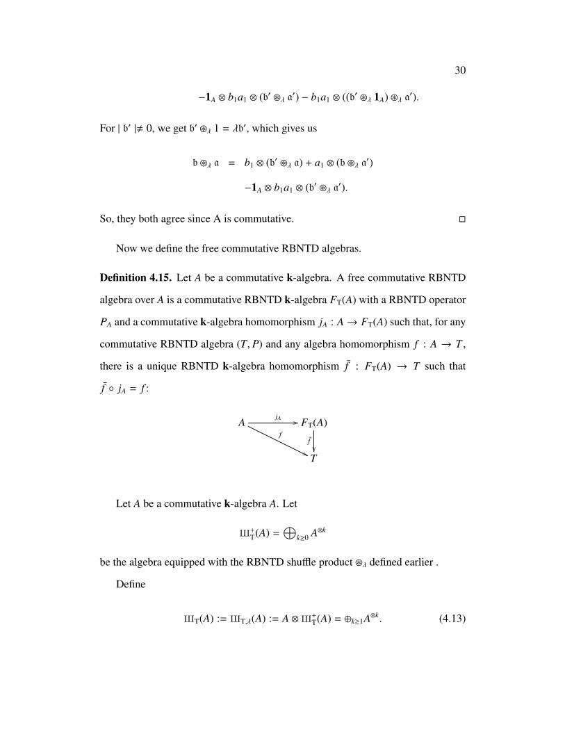
Now we define the free commutative RBNTD algebras.

Definition 4.15. Let A be a commutative k-algebra. A free commutative RBNTD

algebra over A is a commutative RBNTD k-algebra FT(A) with a RBNTD operator

PA and a commutative k-algebra homomorphism jA : A→ FT(A) such that, for any

commutative RBNTD algebra (T, P) and any algebra homomorphism f : A → T ,

there is a unique RBNTD k-algebra homomorphism f : FT(A) → T such that

f ◦ jA = f :

AjA //

f

''

FT(A)

f��

T

Let A be a commutative k-algebra A. Let

X+T(A) =

⊕k≥0 A⊗k

be the algebra equipped with the RBNTD shuffle product ~λ defined earlier .

Define

XT(A) := XT,λ(A) := A ⊗X+T(A) = ⊕k≥1A⊗k. (4.13)

31

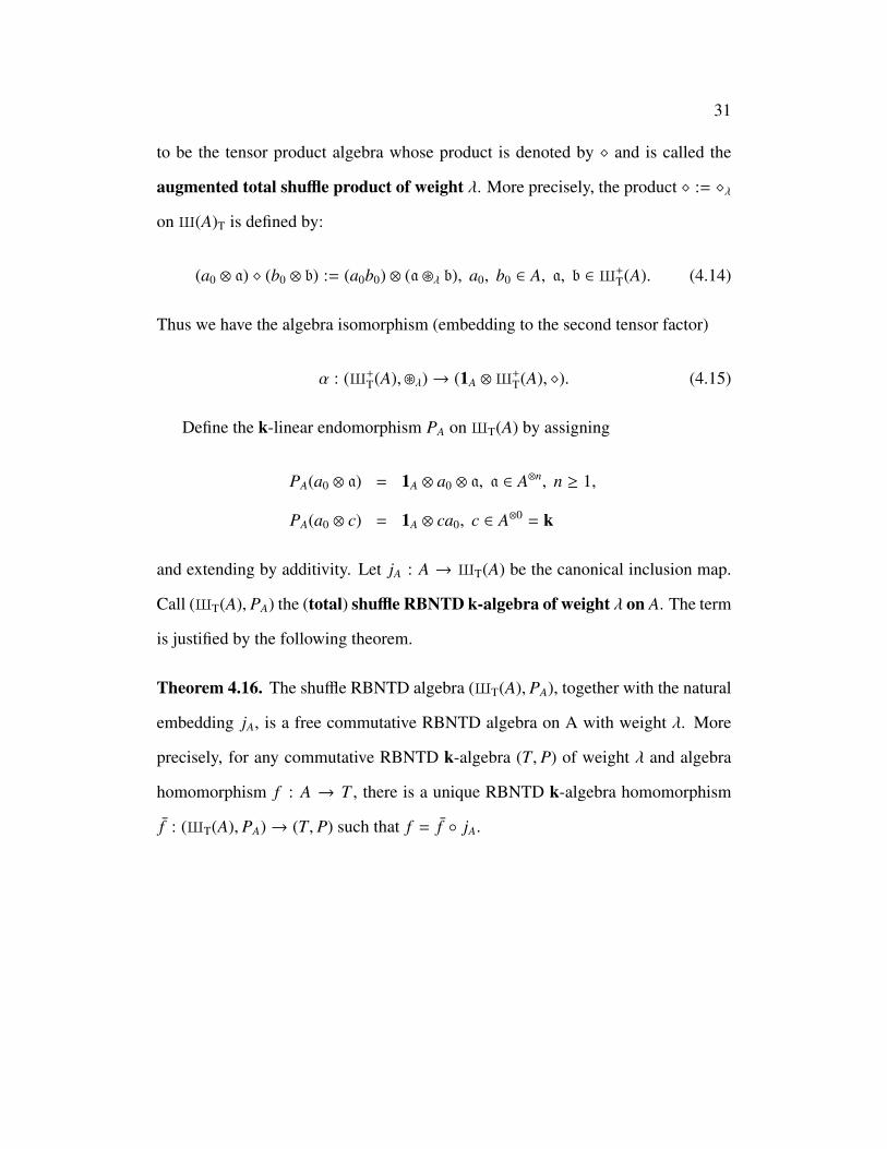
to be the tensor product algebra whose product is denoted by � and is called the

augmented total shuffle product of weight λ. More precisely, the product � := �λ

on X(A)T is defined by:

(a0 ⊗ a) � (b0 ⊗ b) := (a0b0) ⊗ (a ~λ b), a0, b0 ∈ A, a, b ∈X+T(A). (4.14)

Thus we have the algebra isomorphism (embedding to the second tensor factor)

α : (X+T(A),~λ)→ (1A ⊗X+

T(A), �). (4.15)

Define the k-linear endomorphism PA on XT(A) by assigning

PA(a0 ⊗ a) = 1A ⊗ a0 ⊗ a, a ∈ A⊗n, n ≥ 1,

PA(a0 ⊗ c) = 1A ⊗ ca0, c ∈ A⊗0 = k

and extending by additivity. Let jA : A → XT(A) be the canonical inclusion map.

Call (XT(A), PA) the (total) shuffle RBNTD k-algebra of weight λ on A. The term

is justified by the following theorem.

Theorem 4.16. The shuffle RBNTD algebra (XT(A), PA), together with the natural

embedding jA, is a free commutative RBNTD algebra on A with weight λ. More

precisely, for any commutative RBNTD k-algebra (T, P) of weight λ and algebra

homomorphism f : A → T , there is a unique RBNTD k-algebra homomorphism

f : (XT(A), PA)→ (T, P) such that f = f ◦ jA.

32

4.4 The proof of Theorem 4.16

We first prove that (XT(A), PA) is a commutative RBNTD algebra. For pure tensors

a = a1 ⊗ a′ and b = b1 ⊗ b

′,

PA(a) � PA(b) = (1A ⊗ a) � (1A ⊗ b)

= 1A ⊗ (a ~λ b)

= 1A ⊗ (a1 ⊗ (a′ ~λ b)) + 1A ⊗ (b1 ⊗ (a ~λ b′))

+1A ⊗((λa1b1) ⊗ (a′ ~λ b′)) − 1A ⊗ (1A ⊗ a1b1 ⊗ (a′ ~λ b′))

−1A ⊗ (a1b1 ⊗ ((a′ ~λ 1A) ~λ b′))

= PA(a � PA(b)) + PA(b � PA(a)) + λPA(a � b) − P2A(a � b)

−PA((a � PA(1A)) � b).

To verify the universal property of (XT(A), PA), let (T, P) be a commutative RB-

NTD algebra and let f : A → T be an algebra homomorphism. To define f :

XT(A)→ T , we need to define f (a) for any pure tensor a = a1 ⊗ · · · ⊗ an ∈ A⊗n. For

this, we use induction on n. When n = 1, we have A = jA(A). So, we must have

f (a) = f (a). Assume that f (a) has been defined for n ≤ k and let a ∈ A⊗(k+1). Then

a = a1 ⊗ a′ with a′ ∈ A⊗k. Note that a = a1 � PA(a′). Since f is to be a RBNTD

algebra homomorphism, we must have

f (a) = f (a1) f (PA(a′)) = f (a1)P( f (a′)). (4.16)

In fact, if a = a1 ⊗ a2 ⊗ · · · ⊗ ak+1, then we must have

f (a) = f (a1)P(f (a2)P( f (a3) · · · f (ak+1))

).

So the uniqueness of f is proved.

33

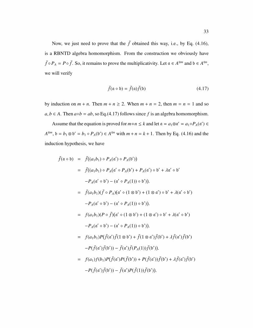
Now, we just need to prove that the f obtained this way, i.e., by Eq. (4.16),

is a RBNTD algebra homomorphism. From the construction we obviously have

f ◦PA = P◦ f . So, it remains to prove the multiplicativity. Let a ∈ A⊗m and b ∈ A⊗n,

we will verify

f (a � b) = f (a) f (b) (4.17)

by induction on m + n. Then m + n ≥ 2. When m + n = 2, then m = n = 1 and so

a, b ∈ A. Then a�b = ab, so Eq.(4.17) follows since f is an algebra homomorphism.

Assume that the equation is proved for m+n ≤ k and let a = a1⊗a′ = a1�PA(a′) ∈

A⊗m, b = b1 ⊗ b′ = b1 � PA(b′) ∈ A⊗n with m + n = k + 1. Then by Eq. (4.16) and the

induction hypothesis, we have

f (a � b) = f((a1b1) � PA(a′) � PA(b′)

)= f

((a1b1) � PA

(a′ � PA(b′) + PA(a′) � b′ + λa′ � b′

−PA(a′ � b′) − (a′ � PA(1)) � b′)).

= f (a1b1)( f ◦ PA)(a′ � (1 ⊗ b′) + (1 ⊗ a′) � b′ + λ(a′ � b′)

−PA(a′ � b′) − (a′ � PA(1)) � b′)).

= f (a1b1)(P ◦ f )(a′ � (1 ⊗ b′) + (1 ⊗ a′) � b′ + λ(a′ � b′)

−PA(a′ � b′) − (a′ � PA(1)) � b′)).

= f (a1b1)P(f (a′) f (1 ⊗ b′) + f (1 ⊗ a′) f (b′) + λ f (a′) f (b′)

−P( f (a′) f (b′)) − f (a′) f (PA(1)) f (b′)).

= f (a1) f (b1)P(f (a′)P( f (b′)) + P( f (a′)) f (b′) + λ f (a′) f (b′)

−P( f (a′) f (b′)) − f (a′)P( f (1)) f (b′)).

34

= f (a1) f (b1)P(f (a′)

)P(f (b′)

)= f (a1)P

(f (a′)

)f (b1)P

(f (b′)

)= f (a) f (b).

This completes the induction and the proof of Theorem 4.16.

4.5 An observation

Recall how Nijenhuis shuffle product (right-shift product in §4.2.2) denoted by

�r is defined. Once again, for two pure tensors a = a1 ⊗ · · · ⊗ am ∈ A⊗m and

b = b1 ⊗ · · · ⊗ bn ∈ A⊗n, where a = a1 ⊗ a′, b = b1 ⊗ b

′, a′ ∈ A⊗(m−1), b′ ∈ A⊗(n−1),

we define

a�rb = a1 ⊗ (a′�rb) + b1 ⊗ (a�rb′) − 1A ⊗ a1b1 ⊗ (a′�rb

′)

Proposition 4.17. For | a |, | b |≥ 1, if | a |> 1 or | b |> 1, then the RBNTD shuffle

product ~λ satisfies the same recursion as the Nijenhuis product �r.

a ~λ b = a1 ⊗ (a′ ~λ b) + b1 ⊗ (a ~λ b′) − 1A ⊗ a1b1 ⊗ (a′ ~λ b′)

Remark. It is interesting to see that, even though the RBNTD product and

Nijenhuis product satisfy the same recursion, they are not the same because of their

different initial conditions.

Proof. We only need to consider the case when | a |>1 because the product is com-

mutative (Theorem 4.14).

For |a |> 1, there are two cases to consider: either |b |= 1 or |b |> 1.

35

Case I: |a |> 1, |b |= 1 i.e. a = a1 ⊗ a′, b = b1 where |a′ |> 0. Then,

a ~λ b = a1 ⊗ (a′ ~λ b) + b1 ⊗ (a ~λ 1k) + λa1b1 ⊗ (a′ ~λ 1k)

−1A ⊗ a1b1 ⊗ (a′ ~λ 1k) − a1b1 ⊗ ((a′ ~λ 1A) ~λ 1k).

Using Lemma 4.11 on the last term and simplifying other terms, we will get

a ~λ b = a1 ⊗ (a′ ~λ b) + b1 ⊗ (a ~λ 1k) + λa1b1 ⊗ a′

−1A ⊗ a1b1 ⊗ (a′ ~λ 1k) − a1b1 ⊗ λa′.

Now, the 3rd and the 5th term will cancel with each other, so we will get

a ~λ b = a1 ⊗ (a′ ~λ b) + b1 ⊗ (a ~λ 1k) − 1A ⊗ a1b1 ⊗ (a′ ~λ 1k),

which is the same as the recursion of a�rb.

Case II: If |a |>1, |b |>1, i.e. a = a1 ⊗ a′, b = b1 ⊗ b

′ where |a′ |> 0, |b′ |> 0, then


−1A ⊗ a1b1 ⊗ (a′ ~λ b′) − a1b1 ⊗ ((a′ ~λ 1A) ~λ b′).

Using Lemma 4.11 on the last term and simplifying other terms, we will get


−1A ⊗ a1b1 ⊗ (a′ ~λ b′) − a1b1 ⊗ (λa′ ~λ b′).

Now, the 3rd and the 5th term will cancel with each other, so we will get

a ~λ b = a1 ⊗ (a′ ~λ b) + b1 ⊗ (a ~λ b′) − 1A ⊗ a1b1 ⊗ (a′ ~λ b′).

which is the same as the recursion of a�rb.

36

�

4.6 A special case of the free commutative RBNTD algebra

As a particular example, we consider XT(k), the free commutative RBNTD k-

algebra on k.

If we choose A = k in the construction of the free commutative RBNTD k-

algebra, then we get

XT(k) =

∞⊕n=0

k⊗(n+1).

Since the tensor product is over k, we have k⊗(n+1) = k1⊗(n+1), where 1⊗(n+1) =

1 ⊗ · · · ⊗ 1︸︷︷︸(n+1)−factors

. In particular, 1⊗1 = 1k is the unit of k. Thus XT(k) is a free k-module

on the basis 1⊗n, n ≥ 1. The following result gives the multiplication table of XT(k).

As a special case of Lemma 4.11, we have

Lemma 4.18. For any m ∈ N≥0,

1A ~λ 1⊗mA = λ1⊗m

A .

Theorem 4.19. For any m, n ∈ N,

1⊗(m+1)A ~λ 1⊗(n+1)

A = λ1⊗(m+n+1)A .

Proof. We will prove this using the induction hypothesis on the sum m + n.

For m + n = 0, the only option we have is m = n = 0,

1A ~λ 1A = λ1A (by the previous lemma).

37

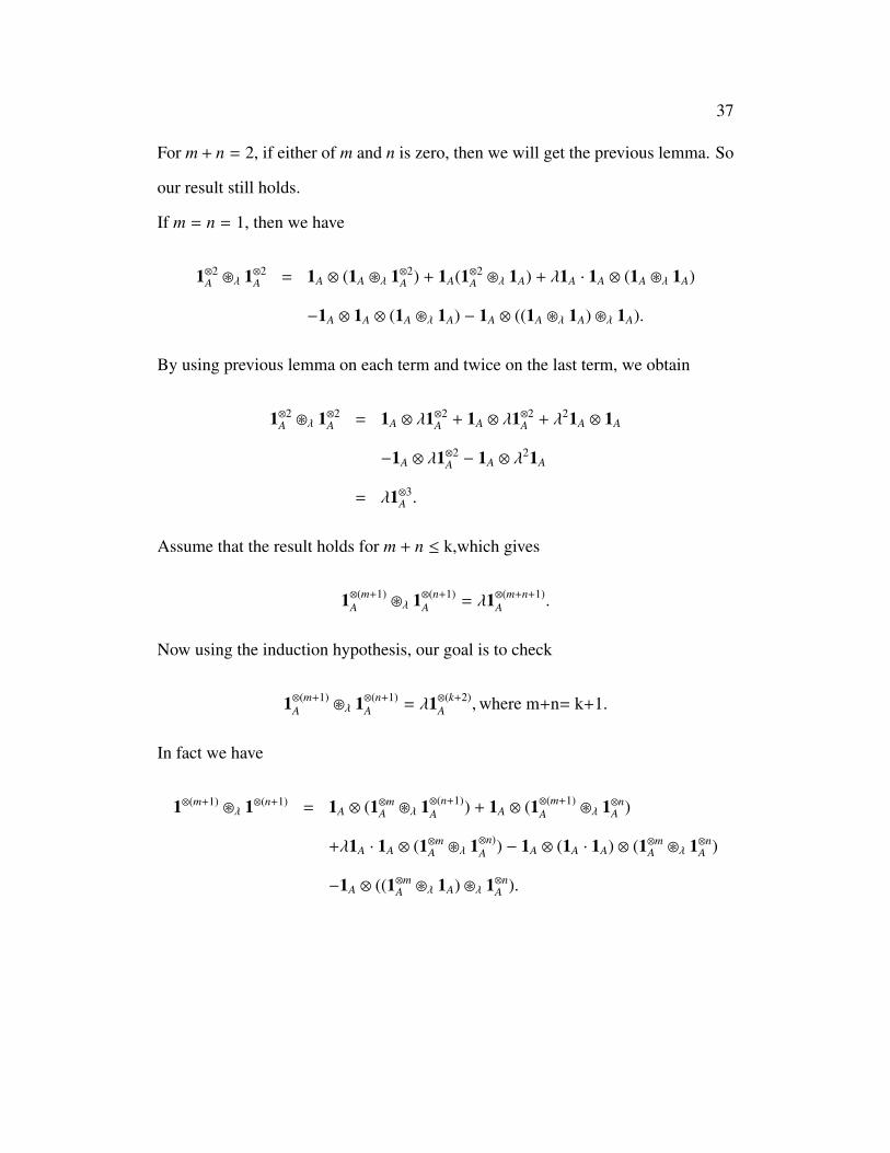
For m + n = 2, if either of m and n is zero, then we will get the previous lemma. So

our result still holds.

If m = n = 1, then we have

1⊗2A ~λ 1⊗2

A = 1A ⊗ (1A ~λ 1⊗2A ) + 1A(1⊗2

A ~λ 1A) + λ1A · 1A ⊗ (1A ~λ 1A)

−1A ⊗ 1A ⊗ (1A ~λ 1A) − 1A ⊗ ((1A ~λ 1A) ~λ 1A).

By using previous lemma on each term and twice on the last term, we obtain

1⊗2A ~λ 1⊗2

A = 1A ⊗ λ1⊗2A + 1A ⊗ λ1⊗2

A + λ21A ⊗ 1A

−1A ⊗ λ1⊗2A − 1A ⊗ λ

21A

= λ1⊗3A .

Assume that the result holds for m + n ≤ k,which gives

1⊗(m+1)A ~λ 1⊗(n+1)

A = λ1⊗(m+n+1)A .

Now using the induction hypothesis, our goal is to check

1⊗(m+1)A ~λ 1⊗(n+1)

A = λ1⊗(k+2)A ,where m+n= k+1.

In fact we have

1⊗(m+1) ~λ 1⊗(n+1) = 1A ⊗ (1⊗mA ~λ 1⊗(n+1)

A ) + 1A ⊗ (1⊗(m+1)A ~λ 1⊗n

A )

+λ1A · 1A ⊗ (1⊗mA ~λ 1⊗n)

A ) − 1A ⊗ (1A · 1A) ⊗ (1⊗mA ~λ 1⊗n

A )

−1A ⊗ ((1⊗mA ~λ 1A) ~λ 1⊗n

A ).

38

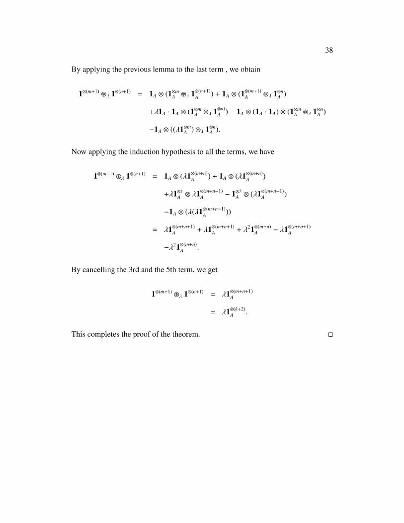
By applying the previous lemma to the last term , we obtain

1⊗(m+1) ~λ 1⊗(n+1) = 1A ⊗ (1⊗mA ~λ 1⊗(n+1)

A ) + 1A ⊗ (1⊗(m+1)A ~λ 1⊗n

A )

+λ1A · 1A ⊗ (1⊗mA ~λ 1⊗n)

A ) − 1A ⊗ (1A · 1A) ⊗ (1⊗mA ~λ 1⊗n

A )

−1A ⊗ ((λ1⊗mA ) ~λ 1⊗n

A ).

Now applying the induction hypothesis to all the terms, we have

1⊗(m+1) ~λ 1⊗(n+1) = 1A ⊗ (λ1⊗(m+n)A ) + 1A ⊗ (λ1⊗(m+n)

A )

+λ1⊗1A ⊗ λ1⊗(m+n−1)

A − 1⊗2A ⊗ (λ1⊗(m+n−1)

A )

−1A ⊗ (λ(λ1⊗(m+n−1)A ))

= λ1⊗(m+n+1)A + λ1⊗(m+n+1)

A + λ21⊗(m+n)A − λ1⊗(m+n+1)

A

−λ21⊗(m+n)A .

By cancelling the 3rd and the 5th term, we get

1⊗(m+1) ~λ 1⊗(n+1) = λ1⊗(m+n+1)A

= λ1⊗(k+2)A .

This completes the proof of the theorem. �

39

5 Free non-commutative RBNTD algebras and

bracketed words

We start with the definition of free RBNTD algebras.

Definition 5.1. Let A be a k-algebra. A free Rota-Baxter Nijenhuis TD algebra over

A is a RBNTD algebra FNCT (A) with a RBNTD operator PA and an algebra homo-

morphism jA : A → FNCT (A) such that, for any RBNTD algebra T and any algebra

homomorphism f : A → T , there is a unique RBNTD algebra homomorphism

f : FNCT (A)→ T such that f ◦ jA = f :

AjA //

f

''

FNCT (A)

f��

T

For the construction of free Rota- Baxter Nijenhuis TD algebras, we follow the

construction of free Rota-Baxter algebras [13, 21] by bracketed words. Alterna-

tively, one can follow [12] to give the construction by rooted trees that is more in

the spirit of operads [30]. We first display a k-basis of the free Rota-Baxter Ni-

jenhuis TD algebra in terms of bracketed words in § 5.1. The product on the free

RBNTD algebra is given in § 5.2 and the universal property of the free RBNTD

algebra is proved in § 5.3.

5.1 A basis of the free RBNTD algebra

For any set X, let S (X) and M(X) denote the free semigroup and free monoid re-

spectively generated by X. For the rest of this chapter , A is taken to be the free

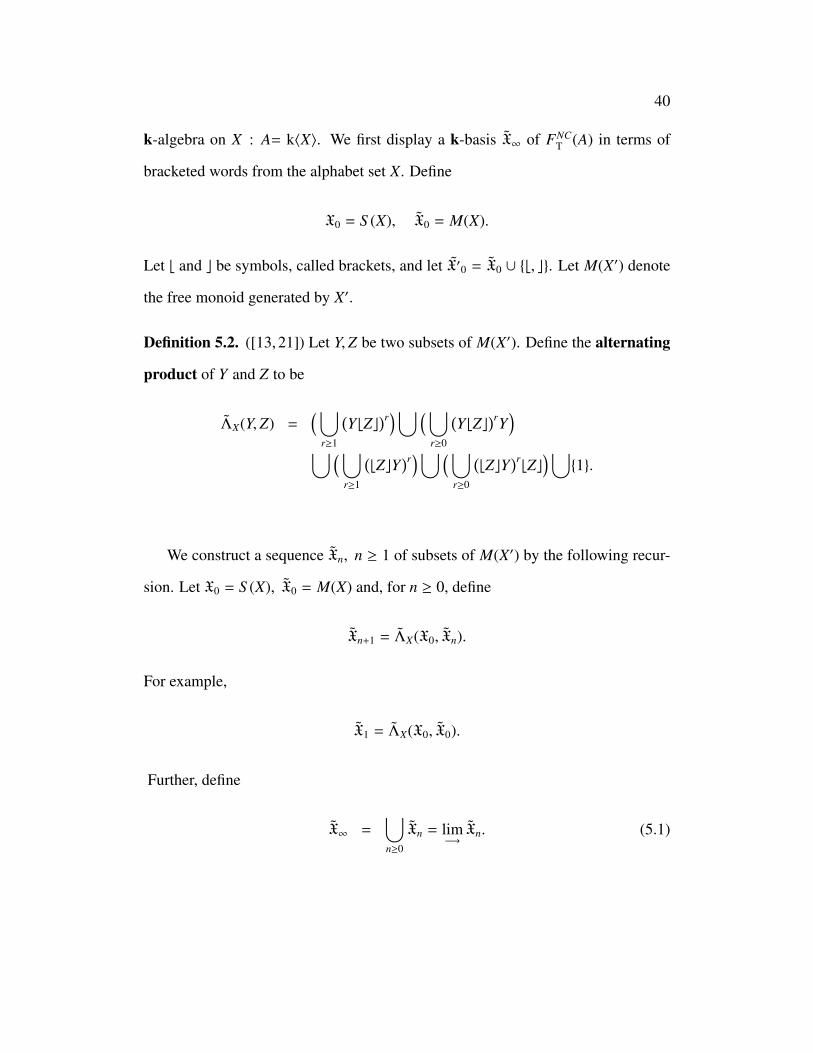
40

k-algebra on X : A= k〈X〉. We first display a k-basis X∞ of FNCT (A) in terms of

bracketed words from the alphabet set X. Define

X0 = S (X), X0 = M(X).

Let b and c be symbols, called brackets, and let X′0 = X0 ∪ {b, c}. Let M(X′) denote

the free monoid generated by X′.

Definition 5.2. ([13, 21]) Let Y,Z be two subsets of M(X′). Define the alternating

product of Y and Z to be

ΛX(Y,Z) =(⋃

r≥1

(YbZc

)r)⋃(⋃

r≥0

(YbZc

)rY)

⋃(⋃r≥1

(bZcY

)r)⋃(⋃

r≥0

(bZcY

)rbZc

)⋃{1}.

We construct a sequence Xn, n ≥ 1 of subsets of M(X′) by the following recur-

sion. Let X0 = S (X), X0 = M(X) and, for n ≥ 0, define

Xn+1 = ΛX(X0, Xn).

For example,

X1 = ΛX(X0, X0).

Further, define

X∞ =⋃n≥0

Xn = lim−→Xn. (5.1)

41

Here the second equation in Eq.(5.1) follows since

X1 ⊇ X0

and, assuming

Xn ⊇ Xn−1,

we have

Xn+1 = ΛX(X0, Xn) ⊇ ΛX(X0, Xn−1) = Xn.

By [13, 21] we have the disjoint union

X∞ =(⊔

r≥1

(X0bX∞c

)r)⊔(⊔

r≥0

(X0bX∞c

)rX0

)⊔(⊔

r≥1

(bX∞cX0

)r)⊔(⊔

r≥0

(bX∞cX0

)rbX∞c

)⋃{1}. (5.2)

Further, every x ∈ X∞ has a unique decomposition

x = x1 · · · xb, (5.3)

where xi, 1 ≤ i ≤ b, is alternatively in X0 or in bX∞c. This decomposition will be

called the standard decomposition of x. For x in X∞ with standard decomposition

x1 · · · xb, we define b to be the breadth b(x) of x, we define the head index h(x) of

x to be 0 (resp. 1) if x1 is in X (resp. in bX∞c). Similarly define the tail index t(x)

of x to be 0 (resp. 1) if xb is in X0 (resp. in bX∞c). The depth d(x) of x in X∞, is the

smallest n ≥ 0 such that x ∈ Xn.

Elements in X∞ are called RBNTD bracketed words.

42

5.2 The product in a free RBNTD algebra

Let

FNCT (A) =

⊕x∈X∞

kx.

We now define a product � on FNCT (A) by defining x � x′ ∈ FNC

T (A) for x, x′ ∈ X∞

and then extending bilinearly. Roughly speaking, the product of x and x′ is defined

to be the concatenation whenever t(x) , h(x′). When t(x) = h(x′), the product is

defined by the product in A or by the RBNTD relation in Eq. (3.4).

To be precise, we use induction on the sum n := d(x) + d(x′) of the depths of x

and x′. Then n ≥ 0. If n = 0, then x, x′ are in X0 and so are in A and we define

x � x′ = x · x′ ∈ A ⊆ FNCT (A).

Here · is the product in A. Suppose x � x′ have been defined for all x, x′ ∈ X∞

with 0 ≤ n ≤ k, and let x, x′ ∈ X∞ with n = k + 1. First assume that the breadth

b(x) = b(x′) = 1. Then x and x′ are in X0 or bX∞c. Since n = k + 1 is at least one, x

and x′ cannot be both in X0. We accordingly define

x � x′ =

xx′, if x ∈ X0, x′ ∈ bX∞c,

xx′, if x ∈ bX∞c, x′ ∈ X0,

bbxc � x′c + bx � bx′cc if x = bxc, x′ = bx′c, x = x1 · · · xb,

+λbx � x′c − bbx � x′cc x′ = x′1 · · · x′

c, xb ∈ X0 and x′1 ∈ X0,

−bxb1cx′c,

bbxc � x′c + bx � bx′cc if x = bxc, x′ = bx′c, x = x1 · · · xb,

−bbx � x′cc, x′ = x′1 · · · x′

c, xb ∈ bX∞c or x′1 ∈ bX∞c.

(5.4)

43

Here, the product in case I and II is by concatenation, whereas, in case III and IV it

is by the induction hypothesis for the four and three products on the right-hand side

respectively, since we have

d(bxc) + d(x′) = d(bxc) + d(bx′c) − 1 = d(x) + d(x′) − 1,

d(x) + d(bx′c) = d(bxc) + d(bx′c) − 1 = d(x) + d(x′) − 1,

d(x) + d(x′) = d(bxc) − 1 + d(bx′c) − 1 = d(x) + d(x′) − 2

which are all less than or equal to k. Now assume b(x) >1 or b(x′) >1. Let x =

x1 · · · xb and x′ = x′1 · · · x′c be the standard decompositions from Eq.(5.3). We then

define

x � x′ = x1 · · · xb−1(xb � x′1) x′2 · · · x′c (5.5)

where xb � x′1 is defined by Eq. (5.4) and the rest is given by concatenation. The

concatenation is well-defined since by Eq. (5.4), we have h(xb) = h(xb � x′1) and

t(x′1) = t(xb � x′1). Therefore, t(xb−1) , h(xb � x′1) and h(x′2) , t(xb � x′1).

We have the following simple properties of �.

Lemma 5.3. Let x, x′ ∈ X∞. We have the following statements.

1. h(x) = h(x � x′) and t(x′) = t(x � x′).

2. If t(x) , h(x′), then x � x′ = xx′ (concatenation).

3. If t(x) , h(x′), then for any x′′ ∈ X∞,

(xx′) � x′′ = x(x′ � x′′), x′′ � (xx′) = (x′′ � x)x′.

44

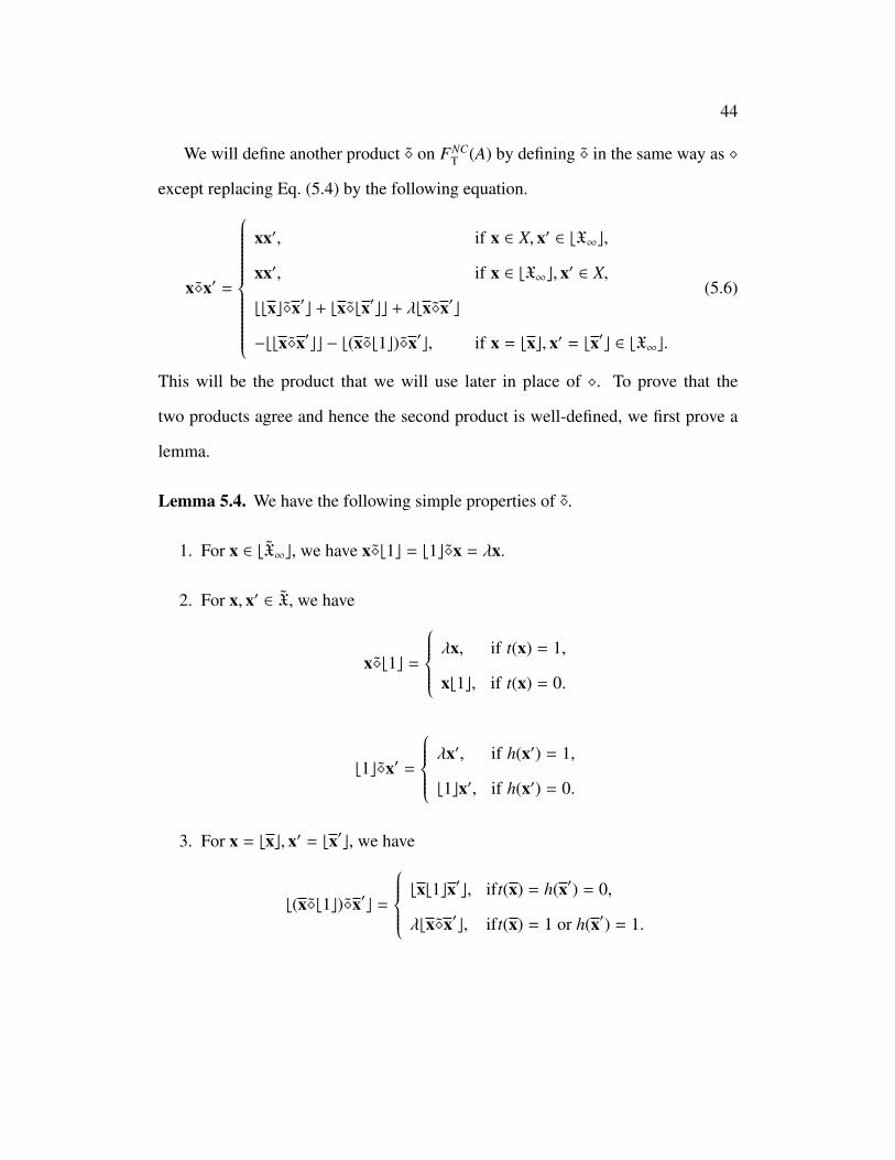
We will define another product � on FNCT (A) by defining � in the same way as �

except replacing Eq. (5.4) by the following equation.

x�x′ =

xx′, if x ∈ X, x′ ∈ bX∞c,

xx′, if x ∈ bX∞c, x′ ∈ X,

bbxc�x′c + bx�bx′cc + λbx�x′c

−bbx�x′cc − b(x�b1c)�x′c, if x = bxc, x′ = bx′c ∈ bX∞c.

(5.6)

This will be the product that we will use later in place of �. To prove that the

two products agree and hence the second product is well-defined, we first prove a

lemma.

Lemma 5.4. We have the following simple properties of �.

1. For x ∈ bX∞c, we have x�b1c = b1c�x = λx.

2. For x, x′ ∈ X, we have

x�b1c =

λx, if t(x) = 1,

xb1c, if t(x) = 0.

b1c�x′ =

λx′, if h(x′) = 1,

b1cx′, if h(x′) = 0.

3. For x = bxc, x′ = bx′c, we have

b(x�b1c)�x′c =

bxb1cx′c, ift(x) = h(x′) = 0,

λbx�x′c, ift(x) = 1 or h(x′) = 1.

45

Proof. (1) Let x = bxc. Then we have

x�b1c = bx�b1cc + bx�1c + λbx�1c − bbx�1cc − b(x�b1c)�1c

= bx�b1cc + bxc + λbxc − bbxcc − bx�b1cc

= λx.

b1c�x = b1�xc + bb1c�xc + λb1�xc − bb1�xcc − bb(1�b1c)�xc

= bxc + bb1c�xc + λbxc − bbxcc − bb1c�xc

= λx.

(2) Let x = x1 · · · xb be the standard decomposition of x. If t(x) = 1 which gives

xb ∈ bX∞c, then x�b1c = λx (from part 1 above). If t(x) = 0 which gives xb ∈ X,

then the product is defined by concatenation. Therefore, we get x�b1c = xb1c.

Similarly, let x′ = x′1 · · · x′c be the standard decomposition of x′. For h(x′) = 1,

x′1 ∈ bX∞c . So b1c�x′ = λx′ (from part 1 above). For h(x′) = 0, x′1 ∈ X, then the

product is defined by concatenation. Therefore, we get b1c�x′ = b1cx′.

(3) For b(x�b1c)�x′c, we need to take three cases:

Case I: When t(x) = h(x′) = 0, then the product is by concatenation. Therefore, we

get b(x�b1c)�x′c = bxb1cx′c.

Case II: When t(x) = 1, then by part 2, we get b(x�b1c)�x′c = λbx�x′c.

Case III: When h(x′) = 1, then also by part 2, we get b(x�b1c)�x′c = λbx�x′c. �

Proposition 5.5. The product � in Eq. (5.4) equals product �.

Proof. Since � and � are defined by the same recursion except their recursive for-

mulas in Eq. (5.6) and Eq. (5.6), we just need to verify that the product � satisfies

46

the same recursion as for � in Eq. (5.4). Applying Lemma 5.4 to the expression

(x � b1c) � x′ in Eq. (5.6), we obtain

x�x′ =

xx′, if x ∈ X, x′ ∈ bX∞c,

xx′, if x ∈ bX∞c, x′ ∈ X,

bbxc�x′c + bx�bx′cc + λbx�x′c

−bbx�x′cc − bxb1cx′c, if t(x) = h(x′) = 0,

bbxc�x′c + bx�bx′cc − bbx�x′cc, if t(x) = 1 or h(x′) = 1.

This is the same recursion as Eq. (5.4). Therefore, � = �. �

Extending � bilinearly, we obtain a binary operation

FNCT (A) ⊗ FNC

T (A)→ FNCT (A).

For x ∈ X∞, define

TA(x) = bxc. (5.7)

Obviously bxc is again in X∞. Thus TA extends to a linear operator TA on FNCT (A).

Let

jX : X → X∞ → FNCT (A)

be the natural injection which extends to an algebra injection

jA : A→ FNCT (A). (5.8)

The following is our main result which will be proved in the next subsection.

Theorem 5.6. Let A be a k-algebra with a k-basis X.

47

1. The pair (FNCT (A), �) is an k-algebra.

2. The triple (FNCT (A), �,TA) is a RBNTD k-algebra.

3. The quadruple (FNCT (A), �,TA, jA) is the free RBNTD algebra on the algebra

A.

The immediate corollary of above theorem will be used in later section.

Corollary 5.7. Let M be a k-module and let T (M) =⊕

n≥0 M⊗n be the tensor

algebra over M. Then FNCT (T (M)), together with the natural injection

iM : M → T (M)jT (M)−−−→ FNC

T (T (M)),

is a free RBNTD algebra over M, in the sense that, for any RBNTD algebra N

and k-module map f : M → N there is a unique RBNTD algebra homomorphism

f : FNCT (T (M))→ N such that f ◦ iM = f .

Proof. This follows immediately from Theorem 5.6 and the fact that the construc-

tion of the free algebra on a module (resp. free RBNTD algebra on an algebra, resp.

free RBNTD on a module) is the left adjoint functor of the forgetful functor from

algebras to modules (resp. from RBNTD algebras to algebras, resp. from RBNTD

algebras to modules), and the fact that the composition of two left adjoint functors

is the left adjoint functor of the composition. �


1. We just need to verify the associativity. For this, we only need to verify

(x′ � x′′) � x′′′ = x′ � (x′′ � x′′′) (5.9)

48

for x′, x′′, x′′′ ∈ X∞. We will do this by induction on the sum of the depths n :=

d(x′) + d(x′′) + d(x′′′). If n = 0, then all of x′, x′′, x′′′ have depth zero and so are

in X. In this case the product � is given by the product · in A and so is associative.

Assume the associativity holds for n ≤ k and assume that x′, x′′, x′′′ ∈ X∞ have

n = d(x′) + d(x′′) + d(x′′′) = k + 1. If t(x′) , h(x′′), then by Lemma 5.3,

(x′ � x′′) � x′′′ = (x′x′′) � x′′′ = x′(x′′ � x′′′) = x′ � (x′′ � x′′′).

A similar argument holds when t(x′′) , h(x′′′). Thus, we only need to verify the as-

sociativity when t(x′) = h(x′′) and t(x′′) = h(x′′′). We will next reduce the breadths

of the words.

Lemma 5.8. If the associativity

(x′ � x′′) � x′′′ = x′ � (x′′ � x′′′)

holds for all x′, x′′ and x′′′ in X∞ of breadth one, then it holds for all x′, x′′ and x′′′

in X∞.

Proof. We use induction on the sum of breadths m := b(x′) + b(x′′) + b(x′′′). Then

m ≥ 3. The case when m = 3 is the assumption of the lemma. Assume that the

associativity holds for 3 ≤ m ≤ j and take x′, x′′, x′′′ ∈ X∞ with m = j + 1. Then

j + 1 ≥ 4. So at least one of x′, x′′, x′′′ have breadth greater than or equal to 2. First

assume b(x′) ≥ 2. Then x′ = x′1x′2 with x′1, x′2 ∈ X∞ and t(x′1) , h(x′2). Thus by

Lemma 5.3, we obtain

(x′ � x′′) � x′′′ = ((x′1x′2) � x′′) � x′′′ = (x′1(x′2 � x′′)) � x′′′ = x′1((x′2 � x′′) � x′′′).

49

Similarly,

x′ � (x′′ � x′′′) = (x′1x′2) � (x′′ � x′′′) = x′1(x′2 � (x′′ � x′′′)).

Thus (x′ � x′′) � x′′′ = x′ � (x′′ � x′′′) whenever (x′2 � x′′) � x′′′ = x′2 � (x′′ � x′′′). The

latter follows from the induction hypothesis. A similar proof works if b(x′′′) ≥ 2.

Finally if b(x′′) ≥ 2, then x′′ = x′′1 x′′2 with x′′1 , x′′2 ∈ X∞ and t(x′′1 ) , h(x′′2 ). By

applying Lemma 5.3 repeatedly, we obtain

(x′ � x′′) � x′′′ = (x′ � (x′′1 x′′2 )) � x′′′ = ((x′ � x′′1 )x′′2 ) � x′′′ = (x′ � x′′1 )(x′′2 � x′′′).

In the same way, we have

(x′ � x′′1 )(x′′2 � x′′′) = x′ � (x′′ � x′′′).

This again proves the associativity. �

To summarize, our proof of the associativity has been reduced to the special

case when x′, x′′, x′′′ ∈ X∞ are chosen so that

1. n := d(x′) + d(x′′) + d(x′′′) = k + 1 ≥ 1 with the assumption that the associa-

tivity holds when n ≤ k.

2. the elements have breadth one and

3. t(x′) = h(x′′) and t(x′′) = h(x′′′).

By 2, the head and tail of each of the elements are the same. Therefore by 3, either

all the three elements are in X or they are all in bX∞c. If all of x′, x′′, x′′′ are in X,

then as already shown, the associativity follows from the associativity in A. Now

50

only case to check is when x′, x′′, x′′′ are all in bX∞c. Then

x′ = bx′c, x′′ = bx′′c, x′′′ = bx′′′c

with x′, x′′, x′′′ ∈ X∞.

For (x′ � x′′) � x′′′, using Eq. (5.6) and bilinearity of the product �, we will get

(bx′c � bx′′c) � bx′′′c =(bbx′c � x′′c + bx′ � bx′′cc + λbx′ � x′′c

−bbx′ � x′′cc − b(x′b1c) � x′′c)� bx′′′c

= (bbx′c � x′′c) � bx′′′c + (bx′ � bx′′cc) � bx′′′c

+(λbx′ � x′′c) � bx′′′c − (bbx′ � x′′cc) � bx′′′c

−(b(x′ � b1c) � x′′c) � bx′′′c

= b(bbx′c � x′′c) � x′′′c + b(bx′c � x′′) � bx′′′cc

+λb(bx′c � x′′) � x′′′c − bb(bx′c � x′′) � x′′′cc

−b((bx′c � x′′) � b1c) � x′′′c + bbx′ � bx′′cc � x′′′c

+b(x′ � bx′′c) � bx′′′cc + λb(x′ � bx′′c) � x′′′c

−bb(x′ � bx′′c) � x′′′cc − b((x′ � bx′′c) � b1c) � x′′′c

+λbbx′ � x′′c � x′′′c + λb(x′ � x′′) � bx′′′cc

+λ2b(x′ � x′′) � x′′′c − λbb(x′ � x′′) � x′′′cc

−λb((x′ � x′′)b1c) � x′′′c − bbbx′ � x′′cc � x′′′c

−bbx′ � x′′c � bx′′′cc − λbbx′ � x′′c � x′′′c

+bbbx′ � x′′c � x′′′cc + b(bx′ � x′′c � b1c) � x′′′c

−bb(x′ � b1c)x′′c � x′′′c − b((x′ � b1c) � x′′) � bx′′′cc

−λb((x′ � b1c) � x′′) � x′′′c + bb((x′ � b1c) � x′′) � x′′′cc

51

+b(((x′ � b1c) � x′′) � b1c) � x′′′c.

Applying the induction hypothesis in n for the 7th and then expanding the 7th and

the 17th term using Eq. (5.6), we obtain

(bx′c � bx′′c) � bx′′′c = bbbx′c � x′′c � x′′′c + b(bx′c � x′′) � bx′′′cc



+bx′ � (bbx′′c � x′′′c)c + bx′ � (bx′′ � bx′′′c)c

+λbx′ � (bx′′ � x′′′c)c − bx′ � (bbx′′ � x′′′cc)c

−bx′ � (b(x′′ � b1c) � x′′′c)c + λb(x′ � bx′′c) � x′′′c

−bb(x′ � bx′′c) � x′′′cc − b((x′ � bx′′c) � b1c) � x′′′c

+λbbx′ � x′′c � x′′′c + λb(x′ � x′′) � bx′′′cc

+λ2b(x′ � x′′) � x′′′c − λbb(x′ � x′′) � x′′′cc

−λb((x′ � x′′) � b1c) � x′′′c − bbbx′ � x′′cc � x′′′c

−bbbx′ � x′′c � x′′′cc − bb(x � x′) � bx′′ccc

−λbb(x′ � x′′) � x′′′cc + bbb(x′ � x′′) � x′′′ccc

+bb((x′ � x′′) � b1c) � x′′′cc − λbbx′ � x′′c � x′′′c

+bbbx′ � x′′c � x′′′cc + b(bx′ � x′′c � b1c) � x′′′c

−bb(x′ � b1c) � x′′c � x′′′c − b((x′ � b1c) � x′′) � bx′′′cc


+b(((x′ � b1c) � x′′) � b1c) � x′′c.

Applying the induction hypothesis in n, using Eq. (5.6) to the 14th and the 28th

52

term, we obtain

b((x′ � bx′′c) � b1c) � x′′′c = b(x′ � (bx′′c � b1c)) � x′′′c

= b(x′ � (bbx′′c � 1c)) � x′′′c + b(x′ � (bx′′ � b1c))c � x′′′c

+λb(x′ � (bx′′ � 1c)) � x′′′c − b(x′ � (bbx′′cc)) � x′′′c

−b(x′ � (b(x′′ � b1c) � 1c)) � x′′′c

b(bx′ � x′′c � b1c) � x′′′c = b(bbx′ � x′′c � 1c) � x′′′c + b(b(x′ � x′′) � b1cc) � x′′′c

+λb(b(x′ � x′′) � 1c) � x′′′c − b(bb(x′ � x′′) � 1cc) � x′′′c

−b(b((x′ � x′′) � b1c) � 1c) � x′′′c.

Substituting these into the original equation, we will get

(bx′c � bx′′c) � bx′′′c = bbbx′c � x′′c � x′′′c + b(bx′c � x′′) � bx′′′cc



+bx′ � (bbx′′c � x′′′c)c + bx′ � (bx′′ � bx′′′c)c

+λbx′ � (bx′′ � x′′′c)c − bx′ � (bbx′′ � x′′′cc)c

−bx′ � (b(x′′ � b1c) � x′′′c)c + λb(x′ � bx′′c) � x′′′c

−bb(x′ � bx′′c) � x′′′cc − b(x′ � (bbx′′c � 1c)) � x′′′c

−b(x′ � (bx′′ � b1c))c � x′′′c − λb(x′ � (bx′′ � 1c)) � x′′′c

+b(x′ � (bbx′′cc)) � x′′′c + b(x′ � (b(x′′ � b1c) � 1c)) � x′′′c

+λb(bx′ � x′′c) � x′′′c + λb(x′ � x′′) � bx′′′cc

53

+λ2b(x′ � x′′) � x′′′c − λbb(x′ � x′′) � x′′′cc

−λb((x′ � x′′)b1c) � x′′′c − bbbx′ � x′′cc � x′′′c

−bbbx′ � x′′c � x′′′cc − bb(x′ � x′′) � bx′′′ccc

−λbb(x′ � x′′) � x′′′cc + bbb(x′ � x′′) � x′′′ccc

+bb((x′ � x′′) � b1c) � x′′′cc − λbbx′ � x′′c � x′′′c

+bbbx′ � x′′c � x′′′cc + b(bbx′ � x′′c � 1c) � x′′′c

+b(b(x′ � x′′) � b1cc) � x′′′c + λb(b(x′ � x′′) � 1c) � x′′′c

−b(bb(x′ � x′′) � 1cc) � x′′′c − b(b((x′ � x′′) � b1c) � 1c) � x′′′c

−bb(x′ � b1c) � x′′c � x′′′c − b((x′ � b1c) � x′′) � bx′′′cc


+b(((x′ � b1c) � x′′) � b1c) � x′′c.

By a similar computation on x′ � (x′′ � x′′′), we obtain

bx′c �(bx′′c � bx′′′c

)= bbbx′c � x′′c � x′′′c + bbx′ � bx′′cc � x′′′c

+λbbx′ � x′′c � x′′′c − bbbx′ � x′′cc � x′′′c

−bb(x′ � b1c) � x′′c � x′′′c + bx′ � (bbx′′c � x′′′c)c

+λbx′ � (bx′′c � x′′′)c − bbx′ � (bx′′c � x′′′)cc

−bx′ � bb1c � x′′c � x′′′c − bx′ � (bbx′′cc � x′′′)c

−λbx′ � (bx′′c � x′′′)c + bx′ � (bbx′′cc � x′′′)c

+bx′ � bb1c � (x′′c � x′′′)c + bbx′c � (x′′ � bx′′′c)c

+bx′ � (bx′′ � bx′′′cc)c + λbx′ � (x′′ � bx′′′c)c

−bbx′ � (x′′ � bx′′′c)cc − b(x′ � b1c) � (x′′ � bx′′′c)c

54

+λbbx′c � (x′′ � x′′′)c + λbx′ � bx′′ � x′′′cc

+λ2bx′ � (x′′ � x′′′)c − λbbx′ � (x′′ � x′′′)cc

−λb(x′ � b1c) � (x′′ � x′′′)c − bbbx′c � (x′′ � x′′′)cc

−bbx′ � (bx′′ � x′′′cc)c − λbbx′ � (x′′ � x′′′)cc

+bbbx′ � (x′′ � x′′′)ccc + bb(x′ � b1c) � (x′′ � x′′′)cc

−bx′ � bbx′′ � x′′′ccc − λbx′ � bx′′ � x′′′cc

+bbx′ � bx′′ � x′′′ccc + bx′ � bb1c � (x′′ � x′′′)cc

+bx′ � bbx′′ � x′′′ccc + λbx′ � bx′′ � x′′′cc

−bx′ � bbx′′ � x′′′ccc − bx′bb1c � (x′′ � x′′′)cc

−bbx′c � ((x′′ � b1c) � x′′′)c − bx′ � b(x′′ � b1c)c � x′′′c

−λbx′ � ((x′′ � b1c) � x′′′)c + bbx′ � ((x′′ � b1c) � x′′′)cc

+b(x′ � b1c) � ((x′′ � b1c) � x′′′)c.

Some of the terms on the left hand side cancel among themselves. Those terms are:

15th and 18th, 25th and 31st, 30th and 34th, 32nd and 35th, 33rd and 36th. After

simplifying, we will get

(bx′c � bx′′c) � bx′′′c = bbbx′c � x′′c � x′′′c︸︷︷︸L1

+ b(bx′c � x′′) � bx′′′cc︸︷︷︸L2

+ λb(bx′c � x′′) � x′′′c︸︷︷︸L3

− bb(bx′c � x′′) � x′′′cc︸︷︷︸L4

− b((bx′c � x′′) � b1c) � x′′′c︸︷︷︸L5

+ b(bx′ � bx′′cc) � x′′′c︸︷︷︸L6

+ bx′ � (bbx′c � x′′c)c︸︷︷︸L7

+ bx′ � (bx′′ � bx′′′cc)c︸︷︷︸L8

+ λbx′ � (bx′′ � x′′′c)c︸︷︷︸L9

− bx′ � (bbx′′ � x′′′cc)c︸︷︷︸L10

55

− bx′ � (b(x′′ � b1c) � x′′′c)c︸︷︷︸L11

+ λb(x′ � bx′′c) � x′′′c︸︷︷︸L12

− bb(x′ � bx′′c) � x′′′cc︸︷︷︸L13

− b(x′ � (bbx′′c � 1c)) � x′′′c︸︷︷︸L14

− λb(x′ � (bx′′ � 1c)) � x′′′c︸︷︷︸L15

+ b(x′ � (bbx′′cc)) � x′′′c︸︷︷︸L16

+ λb(bx′ � x′′c) � x′′′c︸︷︷︸L17

+ λb(x′ � x′′) � bx′′′cc︸︷︷︸L18

+ λ2b(x′ � x′′) � x′′′c︸︷︷︸L19

− λbb(x′ � x′′) � x′′′cc︸︷︷︸L20

− λb((x′ � x′′) � b1c) � x′′′c︸︷︷︸L21

− b(bbx′ � x′′cc) � x′′′c︸︷︷︸L22

− bb(x′ � x′′) � bx′′′ccc︸︷︷︸L23

− λbb(x′ � x′′) � x′′′cc︸︷︷︸L24

+ bbb(x′ � x′′) � x′′′ccc︸︷︷︸L25

+ bb((x′ � x′′) � b1c) � x′′′cc︸︷︷︸L26

− bb((x′ � b1c) � x′′c) � x′′′c︸︷︷︸L27

− b((x′ � b1c) � x′′) � bx′′′cc︸︷︷︸L28

− λb((x′ � b1c) � x′′) � x′′′c︸︷︷︸L29

+ bb((x′ � b1c) � x′′) � x′′′cc︸︷︷︸L30

+ b(((x′ � b1c) � x′′) � b1c) � x′′c︸︷︷︸L31

. (5.10)

Similarly, on the right hand side, there are also some terms which cancel among

themselves: 9th and 13th, 25th and 31st, 29th and 33rd, 30th and 34th, 32nd and

36th.

bx′c �(bx′′c � bx′′′c

)= bbbx′c � x′′c � x′′′c︸︷︷︸

R1

+ bbx′ � bx′′cc � x′′′c︸︷︷︸R2

+ λbbx′ � x′′c � x′′′c︸︷︷︸R3

− bbbx′ � x′′cc � x′′′c︸︷︷︸R4

− bb(x′ � b1c) � x′′c � x′′′c︸︷︷︸R5

+ bx′ � (bbx′′c � x′′′c)c︸︷︷︸R6

+ λbx′ � (bx′′c � x′′′)c︸︷︷︸R7

− bbx′ � (bx′′c � x′′′)cc︸︷︷︸R8

56

− bx′ � (bbx′′cc � x′′′)c︸︷︷︸R9

− λbx′ � (bx′′c � x′′′)c︸︷︷︸R10

+ bx′ � (bbx′′cc � x′′′)c︸︷︷︸R11

+ bbx′c � (x′′ � bx′′′c)c︸︷︷︸R12

+ bx′ � bx′′ � bx′′′ccc︸︷︷︸R13

+ λbx′ � (x′′ � bx′′′c)c︸︷︷︸R14

− bbx′ � (x′′ � bx′′′c)cc︸︷︷︸R15

− b(x′ � b1c) � (x′′ � bx′′′c)c︸︷︷︸R16

+ λbbx′c � (x′′ � x′′′)c︸︷︷︸R17

+ λbx′ � bx′′ � x′′′cc︸︷︷︸R18

+ λ2bx′ � (x′′ � x′′′)c︸︷︷︸R19

− λbbx′ � (x′′ � x′′′)cc︸︷︷︸R20

− λb(x′ � b1c) � (x′′ � x′′′)c︸︷︷︸R21

− bbbx′c � (x′′ � x′′′)cc︸︷︷︸R22

− λbbx′ � (x′′ � x′′′)cc︸︷︷︸R23

+ bbbx′ � (x′′ � x′′′)ccc︸︷︷︸R24

+ bb(x′ � b1c) � (x′′ � x′′′)cc︸︷︷︸R25

− bx′ � bbx′′ � x′′′ccc︸︷︷︸R26

− bbx′c � ((x′′ � b1c) � x′′′)c︸︷︷︸R27

− bx′ � b(x′′ � b1c)c � x′′′c︸︷︷︸R28

− λbx′ � ((x′′ � b1c) � x′′′)c︸︷︷︸R29

+ bbx′ � ((x′′ � b1c) � x′′′)cc︸︷︷︸R30

+ b(x′ � b1c) � ((x′′ � b1c) � x′′′)c︸︷︷︸R31

. (5.11)

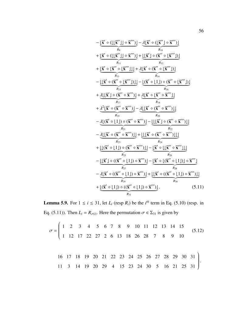
Lemma 5.9. For 1 ≤ i ≤ 31, let Li (resp Ri) be the ith term in Eq. (5.10) (resp. in

Eq. (5.11)). Then Li = Rσ(i). Here the permutation σ ∈ Σ31 is given by

σ =

1 2 3 4 5 6 7 8 9 10 11 12 13 14 15

1 12 17 22 27 2 6 13 18 26 28 7 8 9 10(5.12)

16 17 18 19 20 21 22 23 24 25 26 27 28 29 30 31

11 3 14 19 20 29 4 15 23 24 30 5 16 21 25 31

.

57

This permuation is too long to fit in one line, so is split into two.

Proof. We divide the proof of this lemma by type of terms into three cases:

Case I: Those terms on the left hand side i.e. in Eq. (5.10) that exactly match with

certain terms on the right hand side i.e. Eq. (5.11) . They are:

L1 = R1, L6 = R2, L7 = R6, L8 = R13, L9 = R18, L10 = R26, L17 = R3, L22 = R4

Case II: Those terms on the left hand side that match with the right hand side using

induction on sum of depths of x′, x′′, x′′′ i.e. d(x′) + d(x′′) + d(x′′′) ≤ n + 1. They

are:

L2 = R12, L3 = R17, L4 = R22, L12 = R7, L13 = R8, L14 = R9, L15 = R10, L16 = R11,

L18 = R14, L19 = R19, L20 = R20, L23 = R15, L24 = R23, L25 = R24

Case III: Those remaining terms that we want match are the special terms in which

b1c is involved. They are :

L5 = R27, L11 = R28, L21 = R29, L26 = R30, L27 = R5, L28 = R16, L29 = R21, L30 = R25,

L31 = R31 .

We only need to verify Case III. Before we check that these terms match, we need

two claims.

Lemma 5.10. For all x′, x′′ ∈ M(X), (x′ � x′′) � b1c = x′ � (x′′ � b1c).

Proof. We will prove the result by induction on n: n = d(x′) + d(x′′) ≥0.

For n=0, x′, x′′ ∈ M(X), x′ = x1x2 · · · xk,

(x′ � x′′) � b1c = (x1 · · · xkx′′) � b1c = x1 · · · xk(x′′ � b1c) = x′ � (x′′ � b1c).

Assume the result holds for n≤ k. Consider n = d(x′) + d(x′′) = k + 1.

If either x′ or x′′ has depth 0, then the result holds from n=0 case. Otherwise,

58

x′ = bx′c, then the using induction hypothesis, we have

(x′ � x′′) � b1c = (bx′c � x′′) � b1c = bx′c � (x′′ � b1c) = x′ � (x′′ � b1c).

�

Claim 5.11. For x ∈ X∞, d(x � b1c) ≤ d(x) + 1, where d(x)=depth of x.

Proof. Let x = x1 · · · xk, xi ∈ X⊔bM(X)c. If xk = x ∈ X, then x � b1c = x1 · · · xkb1c.

This gives us : d(x � b1c)=max{d(x), d(b1c)} ≤ d(x) + 1.

When xk = bxkc , then d(xk � b1c) ≤ d(xk ) +1 (by definition of �). Now, d(x � b1c)

= d((x1 · · · xk) � b1c).

Now by lemma 5.3, d((x1 · · · xk) � b1c) =d(x1 · · · xk−1(xk � b1c)), hence we get

d(x � b1c) = d(x1 · · · xk−1(xk � b1c))

= max{d(x1), · · · , d(xk � b1c)}

≤ max{d(x1), · · · , d(xk) + 1}

≤ max{d(x1) + 1, · · · , d(xk) + 1}

= max{d(x1), · · · , d(xk)} + 1

= d(x) + 1.

This proves the claim. �

Now, coming back to our lemma, we will check some of them since the proofs

are similar:

L5 = b((bx′c � x′′) � b1c) � x′′′c

= b(bx′c � (x′′ � b1c)) � x′′′c (By claim (5.10) and the induction hypothesis)

= bbx′c � ((x′′ � b1c) � x′′′)c (By claim (5.11) and the induction hypothesis)

59

= R27.

L21 = b((x′ � x′′) � b1c) � x′′′c

= b(x′ � (x′′ � b1c)) � x′′′c (By claim (5.10) and the induction hypothesis)

= bx′ � ((x′′ � b1c) � x′′′)c (By claim (5.11) and the induction hypothesis)

= R29.

L31 = b(((x′ �b1c)�x′′)�b1c)�x′′c (By claim (5.10) and the induction hypothesis)

= b((x′�b1c)�(x′′�b1c))�x′′′c (By claim (5.10) and the induction hypothesis)

= b(x′ � b1c) � ((x′′ � b1c) � x′′′)c

= R31. �

This completes the proof of Theorem 5.6.1.

2. The proof follows from the definition TA(x) = bxc and Eq. (5.6).

3. Let (T, ∗, P) be a RBNTD algebra with multiplication ∗. Let f : A → T be a

k-algebra homomorphism. We will construct a k-linear map f : FNCT (A) → T by

defining f (x) for x ∈ X∞. We achieve this by defining f (x) for x ∈ Xn, n ≥ 0,

inductively on n. For x ∈ X0 := X, define f (x) = f (x). Suppose f (x) has been

defined for x ∈ Xn and consider x in Xn+1 which is, by definition and Eq. (5.2),

ΛX(X,Xn) =(⊔

r≥1

(XbXnc)r)⊔(⊔

r≥0

(XbXnc)rX)

⊔(⊔r≥0

bXnc(XbXnc)r)⊔(⊔

r≥0

bXnc(XbXnc)rX).

Let x be in the first union component⊔

r≥1(XbXnc)r above. Then

x =

r∏i=1

(x2i−1bx2ic)

for x2i−1 ∈ X and x2i ∈ Xn, 1 ≤ i ≤ r. By the construction of the multiplication �

60

and the RBNTD operator TA, we have

x = �ri=1(x2i−1 � bx2ic) = �r

i=1(x2i−1 � TA(x2i)).

Define

f (x) = ∗ri=1

(f (x2i−1) ∗ T

(f (x2i))

). (5.13)

where the right hand side is well-defined by the induction hypothesis. Similarly

define f (x) if x is in the other union components. For any x ∈ X∞, we have TA(x) =

bxc ∈ X∞, and by the definition of f in Eq.(5.13), we have

f (bxc) = P( f (x)). (5.14)

So f commutes with the RBNTD operators. Combining this equation with Eq. (5.13)

we see that if x = x1 · · · xb is the standard decomposition of x, then

f (x) = f (x1) ∗ · · · ∗ f (xb). (5.15)

Note that this is the only possible way to define f (x) in order for f to be a

RBNTD algebra homomorphism extending f .

It remains to prove that the map f defined in Eq. (5.13) is indeed an algebra

homomorphism. For this we only need to check the multiplicity

f (x � x′) = f (x) ∗ f (x′) (5.16)

for all x, x′ ∈ X∞. For this, we use induction on the sum of depths n := d(x) + d(x′).

Then n ≥ 0. When n = 0, we have x, x′ ∈ X. Then Eq. (5.16) follows from the

multiplicity of f . Assume the multiplicity holds for x, x′ ∈ X∞ with n ≥ k and take

61

x, x′ ∈ X∞ with n = k + 1. Let x = x1 · · · xb and x′ = x′1 · · · x′c be the standard

decompositions. Since n = k + 1 ≥ 1, at least one of xb and x′c is in bX∞c. Then by

Eq. (5.6) we have,

f (xb � x′1) =

f (xbx′1), if xb ∈ X, x′1 ∈ bX∞c,

f (xbx′1), if xb ∈ bX∞c, x′1 ∈ X,

f(bbxbc � x′1c + bxb � bx′1cc + λbxb � x′1c

−bbxb � x′1cc − b(xb � b1c) � x′1c), if xb = bxbc, x′1 = bx′1c ∈ bX∞c.

In the first two cases, the right hand side is f (xb) ∗ f (x′1) by the definition of f . In

the third case, we have, by Eq. (5.14), the induction hypothesis and the RBNTD

relation of the operator P on T ,

f(bbxbc � x′1c + bxb � bx′1cc + λbxb � x′1c − bbxb � x′1cc − b(xb � b1c) � x′1c

)= f (bbxbc � x′1c) + f (bxb � bx′1cc) + λ f

(bxb � x′1c

)− f (bbxb � x′1cc) − f

(b(xb � b1c) � x′1c

)=P( f (bxbc � x′1)) + P( f (xb � bx′1c)) + λP( f (xb � x′1c)

− P( f (bxb � x′1c)) − P( f ((xb � b1c) � x′1)

=P( f (bxbc) ∗ f (x′1)) + P( f (xb) ∗ f (bx′1c))

+ λP( f (xb) ∗ P((x′1)) − P(P( f (xb) ∗ f (x′1))) − P( f (xb � b1c) ∗ P( f x′1)

=P(P( f (xb)) ∗ f (x′1)) + P( f (xb) ∗ P( f (x′1)))

+ λP( f (xb) ∗ P((x′1)) − P(P(( f (xb) ∗ f (x′1))) − P( f (xb � b1c) ∗ P( f x′1))

=P( f (xb)) ∗ P( f (x′1))

= f (bxbc) ∗ f (bx′1c)

= f (xb) ∗ f (x′1).

62

Therefore f (xb � x′1) = f (xb) ∗ f (x′1). Then

f (x � x′) = f(x1 · · · xb−1(xb � x′1)x′2 · · · x

′c)

= f (x1) ∗ · · · ∗ f (xb−1) ∗ f (xb � x′1) ∗ f (x′2) · · · f (x′c)

= f (x1) ∗ · · · ∗ f (xb−1) ∗ f (xb) ∗ f (x′1) ∗ f (x′2) · · · f (x′c)

= f (x) ∗ f (x′).

This proves our result.

63

6 RBNTD algebras and RBNTD-dendriform algebras

We first introduce the concepts of a dendriform algebra and a tridendriform algebra

and recall some results from the links between a Rota-Baxter algebra and the den-

driform and the tridendriform algebra [21]. We then determine the binary quadratic

nonsymmetric algebra called the RBNTD-dendriform algebra that is compatible

with the RBNTD-algebra.

In this section, k is a commutative unitary ring.

6.1 Dendriform algebras and tridendriform algebras

The concept of a dendriform algebra was introduced by Loday [28] in 1995 with

motivation from algebraic K-theory.

Definition 6.1. ([28]) A dendriform k-algebra (previously also called a dendri-

form dialgebra) is a k-module D with two binary operations ≺ and � that satisfy the

following relations.

(x ≺ y) ≺ z = x ≺ (y ≺ z + y � z),

(x � y) ≺ z = x � (y ≺ z), x, y, z ∈ D, (6.1)

(x ≺ y + x � y) � z = x � (y � z).

Dendriform algebras have been further studied with connections to several areas

in mathematics and physics, including operads, homological algebra, Hopf algebra,

Lie and Leibniz algebra, combinatorics, arithmetic and quantum field theory.

A few years later, Loday and Ronco defined the tridendriform algebra in their

study [29] of polytopes and Koszul duality.

64

Definition 6.2. ([29]) A tridendriform k-algebra (previously also called a dendri-

form trialgebra) is a k-module T equipped with three binary operations ≺,� and ·

that satisfy the following relations.

(x ≺ y) ≺ z = x ≺ (y ? z),

(x � y) ≺ z = x � (y ≺ z),

(x ? y) � z = x � (y � z),

(x � y) · z = x � (y · z), x, y, z ∈ T, (6.2)

(x ≺ y) · z = x · (y � z),

(x · y) ≺ z = x · (y ≺ z),

(x · y) · z = x · (y · z).

Here we have used the notation

x ? y := x ≺ y + x � y + x · y (6.3)

Proposition 6.3. 1. Let (D,≺,�) be a dendriform algebra. The operation ? :=

?D on D defined by

x ? y := x ≺ y + x � y, x, y ∈ D, (6.4)

is associative.

2. Let (T,≺,�, ·) be a tridendriform algebra. The operation ? := ?T on T de-

65

fined by

x ? y := x ≺ y + x � y + x · y, x, y ∈ T, (6.5)

is associative.

Thus, a dendriform algebra and tridendriform algebra share the property that the

sum of the binary operations ? :=≺ + � for a dendriform algebra or ? :=≺ + � +·

for a tridendriform algebra is associative. Such a property is called a “splitting the

associativity”.

Proof. We just prove Item 1. The proof of Item 2 is similar.

Adding the left hand sides of Eqs. (6.1) , we obtain

(x ≺ y) ≺ z + (x � y) ≺ z + (x ≺ y + x � y) � z

=(x ≺ y + x � y) ≺ z + (x ≺ y + x � y) � z

=(x ? y) ≺ z + (x ? y) � z

=(x ? y) ? z.

Similarly, adding the right hand sides of these equations, we obtain x? (y? z). Thus

we have proved the associativity of ?. �

There is a link between Rota-Baxter algebras and dendriform algebras stated in

the following theorem.

Theorem 6.4. 1. [1] A Rota-Baxter algebra (R, P) of weight zero defines a den-

driform algebra (R,≺P,�P), where

x ≺P y = xP(y), x �P y = P(x)y, ∀x, y ∈ R. (6.6)

66

2. [10] A Rota-Baxter algebra (R, P) of weight λ defines a tridendriform algebra

(R,≺P,�P, ·P), where

x ≺P y = xP(y), x �P y = P(x)y, x ·P y = λxy, ∀x, y ∈ R. (6.7)

6.2 RBNTD-dendriform algebras

Suppose (T, P) is a RBNTD algebra and define binary operations [21, 23]:

x ≺P y = xP(y), x �P y = P(x)y, x ·P y = λxy, x •P y = −P(xy), x ∗P y = −xP(1)y

(6.8)

Our question is, what quadratic nonsymmetric relations could (T,≺P,�P, ·P, •P, ∗P)

satisfy? We recall some background on binary quadratic nonsymmetric operads in

order to make the question precise. We then determine all the quadratic nonsym-

metric relations that are consistent with the RBNTD operator. For details on binary

quadratic nonsymmetric operads, see [21, 30].

Definition 6.5. Let k be a field.

1. A graded vector space is a sequence P :=⊕n≥0Pn of k-vector spaces Pn, n ≥

0.

2. A nonsymmetric (ns) operad is a graded vector space P =⊕n≥0Pn equipped

with partial compositions:

◦i := ◦m,n,i : Pm ⊗ Pn −→ Pm+n−1, 1 ≤ i ≤ m, (6.9)

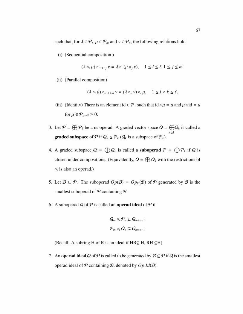
67

such that, for λ ∈ P`, µ ∈ Pm and ν ∈ Pn, the following relations hold.

(i) (Sequential composition )

(λ ◦i µ) ◦i−1+ j ν = λ ◦i (µ ◦ j ν), 1 ≤ i ≤ `, 1 ≤ j ≤ m.

(ii) (Parallel composition)

(λ ◦i µ) ◦k−1+m ν = (λ ◦k ν) ◦i µ, 1 ≤ i < k ≤ `.

(iii) (Identity) There is an element id ∈ P1 such that id◦µ = µ and µ◦ id = µ

for µ ∈ Pn, n ≥ 0.

3. Let P =⊕Pk be a ns operad. A graded vector space Q =

⊕k≥1Qk is called a

graded subspace of P if Qk ≤ Pk (Qk is a subspace of Pk).

4. A graded subspace Q =⊕Qk is called a suboperad P =

⊕Pk if Q is

closed under compositions. (Equivalently, Q =⊕Qk with the restrictions of

◦i is also an operad.)

5. Let B ⊆ P. The suboperad Op(B) = OpP(B) of P generated by B is the

smallest suboperad of P containing B.

6. A suboperad Q of P is called an operad ideal of P if

Qm ◦i Pn ⊆ Qm+n−1

Pm ◦i Qn ⊆ Qm+n−1

(Recall: A subring H of R is an ideal if HR⊆ H, RH ⊆H)

7. An operad idealQ ofP is called to be generated byB ⊆ P ifQ is the smallest

operad ideal of P containing B, denoted by Op Id(B).

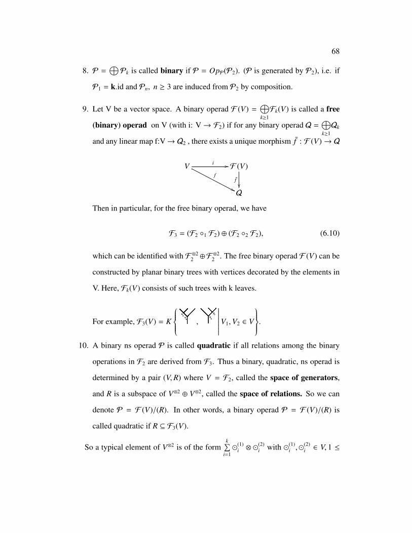
68

8. P =⊕Pk is called binary if P = OpP(P2). (P is generated by P2), i.e. if

P1 = k.id and Pn, n ≥ 3 are induced from P2 by composition.

9. Let V be a vector space. A binary operad F (V) =⊕k≥1Fk(V) is called a free

(binary) operad on V (with i: V→ F2) if for any binary operad Q =⊕k≥1Qk

and any linear map f:V→ Q2 , there exists a unique morphism f : F (V)→ Q

V i //

f

''

F (V)

f��Q

Then in particular, for the free binary operad, we have

F3 = (F2 ◦1 F2) ⊕ (F2 ◦2 F2), (6.10)

which can be identified with F ⊗22 ⊕F

⊗22 . The free binary operad F (V) can be

constructed by planar binary trees with vertices decorated by the elements in

V. Here, Fk(V) consists of such trees with k leaves.

For example, F3(V) = K

,

∣∣∣∣∣∣∣∣ V1,V2 ∈ V

.

10. A binary ns operad P is called quadratic if all relations among the binary

operations in F2 are derived from F3. Thus a binary, quadratic, ns operad is

determined by a pair (V,R) where V = F2, called the space of generators,

and R is a subspace of V⊗2 ⊕ V⊗2, called the space of relations. So we can

denote P = F (V)/(R). In other words, a binary operad P = F (V)/(R) is

called quadratic if R ⊆ F3(V).

So a typical element of V⊗2 is of the formk∑

i=1�

(1)i ⊗ �

(2)i with �(1)

i ,�(2)i ∈ V, 1 ≤

69

i ≤ k.

Thus a typical element of V⊗2 ⊕ V⊗2 is of the form

k∑i=1

�(1)i ⊗ �

(2)i ,

m∑j=1

�(3)j ⊗ �

(4)j

, �(1)i ,�(2)

i ,�(3)j ,�

(4)j ∈ V, 1 ≤ i ≤ k, 1 ≤ j ≤ m, k,m ≥ 1.

For a given binary quadratic ns operad P = P(V)/(R), a k-vector space A is called

a P-algebra if A has binary operations (indexed by) V and if, for

( k∑i=1

�(1)i ⊗ �

(2)i ,

m∑j=1

�(3)j ⊗ �

(4)j)∈ R ⊆ V⊗2 ⊕ V⊗2

with �(1)i ,�(2)

i ,�(3)j ,�

(4)j ∈ V , 1 ≤ i ≤ k, 1 ≤ j ≤ m, we have

k∑i=1

(x �(1)i y) �(2)

i z =

m∑j=1

x �(3)j (y �(4)

j z), ∀ x, y, z ∈ A. (6.11)

Theorem 6.6. Let V = k{≺,�, ·, •, ∗} be the vector space with basis

{≺,�, , ·, •, ∗} and let P = P(V)/(R) be a binary quadratic ns operad. The following

statements are equivalent.

1. For every RBNTD algebra (T, P), the hextuple (T,≺P,�P, ·P, •P, ∗P) is a P-

algebra.

2. The relation space R of P is contained in the subspace of V⊗2 ⊕ V⊗2 spanned

by

(≺ ⊗ ≺,≺ ⊗?), (� ⊗?,� ⊗ �), (≺ ⊗·, ·⊗ �), (6.12)

(≺ ⊗•, •⊗ �), (≺ ⊗∗, ∗⊗ �), (� ⊗ ≺,� ⊗ ≺),

(� ⊗·,� ⊗·), (� ⊗∗,� ⊗∗), (·⊗ ≺, ·⊗ ≺),

70

(· ⊗ ·, · ⊗ ·), (· ⊗ ∗, · ⊗ ∗), (• ⊗ ∗, • ⊗ ∗),

(∗⊗ ≺, ∗⊗ ≺), (∗ ⊗ ·, ∗ ⊗ ·), (∗ ⊗ ∗, ∗ ⊗ ∗), (∗ ⊗ ·,− · ⊗•),

(� ⊗ • + • ⊗ ≺ + • ⊗ • − · ⊗ • + ∗ ⊗•,� ⊗ • + • ⊗ ≺ + • ⊗ • − • ⊗ · + • ⊗∗)

where ? =≺ + � + · + • +∗ . More precisely, any P-algebra A satisfies the

relations

(x ≺ y) ≺ z = x ≺ (y ? z), (x ? y) � z = x � (y � z), (x ≺ y) · z = x · (y � z),

(x ≺ y) • z = x • (y � z), (x ≺ y) ∗ z = x ∗ (y � z), (x � y) ≺ z = x � (y ≺ z),

(x � y) · z = x � (y · z), (x � y) ∗ z = x � (y ∗ z), (x · y) ≺ z = x · (y ≺ z),

(x · y) · z = x · (y · z), (x · y) ∗ z = x · (y ∗ z), (x • y) ∗ z = (x • y) · z,

(x ∗ y) ≺ z = x ∗( y ≺ z), (x ∗ y) · z = x ∗ (y · z), (x ∗ y) ∗ z = x ∗ (y ∗ z),

x ∗ (y · z) = −x · (y • z), ∀x, y, z ∈ A (6.13)

(x � y) • z + (x • y) ≺ z + (x • y) • z − (x · y) • z + (x ∗ y) • z

= x � (y • z) + x • (y ≺ z) + x • (y • z) − x • (y · z) + x • (y ∗ z)

Note that the relations of the dendriform in Eq. (6.1) and the tridendriform in

Eq. (6.2) is contained in the space spanned by the relations in Eq. (6.12). We call

P defined by the relations in Eq. 6.12 the RBNTD-dendriform operad and call

a hextuple (T,≺,�, ·, •, ∗) satisfying Eq. (6.13) an RBNTD-dendriform algebra.

Let RBNTDD denote the category of RBNTD-dendriform algebras and RBNTDA

be the category of RBNTD algebras.

Then we have the following immediate corollary of Theorem 6.6.

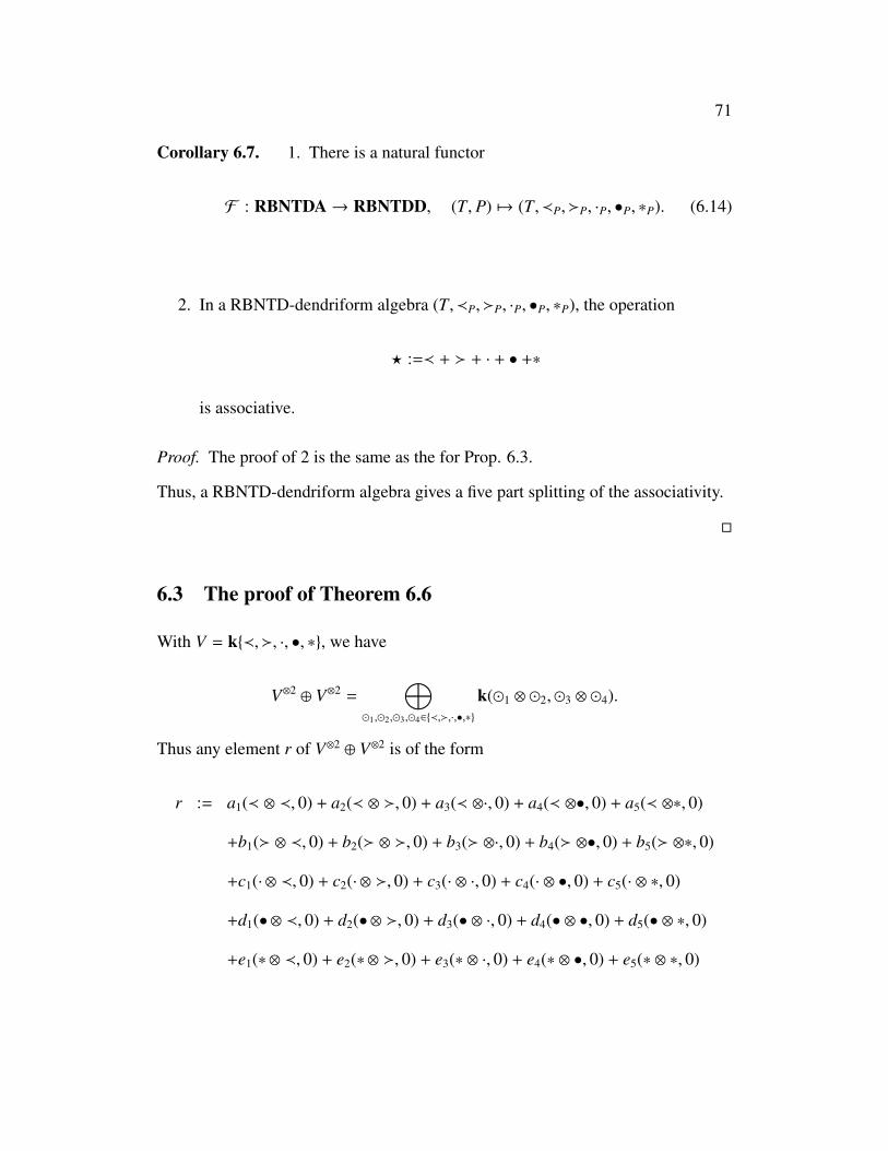
71

Corollary 6.7. 1. There is a natural functor

F : RBNTDA→ RBNTDD, (T, P) 7→ (T,≺P,�P, ·P, •P, ∗P). (6.14)

2. In a RBNTD-dendriform algebra (T,≺P,�P, ·P, •P, ∗P), the operation

? :=≺ + � + · + • +∗

is associative.

Proof. The proof of 2 is the same as the for Prop. 6.3.

Thus, a RBNTD-dendriform algebra gives a five part splitting of the associativity.

�


With V = k{≺,�, ·, •, ∗}, we have

V⊗2 ⊕ V⊗2 =⊕

�1,�2,�3,�4∈{≺,�,·,•,∗}

k(�1 ⊗ �2,�3 ⊗ �4).

Thus any element r of V⊗2 ⊕ V⊗2 is of the form

r := a1(≺ ⊗ ≺, 0) + a2(≺ ⊗ �, 0) + a3(≺ ⊗·, 0) + a4(≺ ⊗•, 0) + a5(≺ ⊗∗, 0)

+b1(� ⊗ ≺, 0) + b2(� ⊗ �, 0) + b3(� ⊗·, 0) + b4(� ⊗•, 0) + b5(� ⊗∗, 0)

+c1(· ⊗ ≺, 0) + c2(· ⊗ �, 0) + c3(· ⊗ ·, 0) + c4(· ⊗ •, 0) + c5(· ⊗ ∗, 0)

+d1(•⊗ ≺, 0) + d2(•⊗ �, 0) + d3(• ⊗ ·, 0) + d4(• ⊗ •, 0) + d5(• ⊗ ∗, 0)

+e1(∗ ⊗ ≺, 0) + e2(∗ ⊗ �, 0) + e3(∗ ⊗ ·, 0) + e4(∗ ⊗ •, 0) + e5(∗ ⊗ ∗, 0)

72

+ f1(0,≺ ⊗ ≺) + f2(0,≺ ⊗ �) + f3(0,≺ ⊗·) + f4(0,≺ ⊗•) + f5(0,≺ ⊗∗)

+g1(0,� ⊗ ≺) + g3(0,� ⊗ �) + g3(0,� ⊗·) + g4(0,� ⊗•) + g5(0,� ⊗∗)

+h1(0, ·⊗ ≺) + h2(0, ·⊗ �) + h3(0, · ⊗ ·) + h4(0, · ⊗ •) + h5(0, · ⊗ ∗)

+i1(0, •⊗ ≺) + i2(0, •⊗ �) + i3(0, • ⊗ ·) + i4(0, • ⊗ •) + i5(0, • ⊗ ∗)

+ j1(0, ∗⊗ ≺) + j2(0, ∗⊗ �) + j3(0, ∗ ⊗ ·) + j4(0, ∗ ⊗ •) + j5(0, ∗ ⊗ ∗)

where the coefficients are in k.

(1 ⇒ 2) Let P = P(V)/(R) be an operad satisfying the condition in Item 1. Let

r be in R expressed in the above form. Then for any RBNTD algebra (T, P), the

hextuple (T,≺P,�P, ·P, •P, ∗P) is a P-algebra. Thus

a1(x ≺P y) ≺P z + a2(x ≺P y) �P z + a3(x ≺P y) ·P z + a4(x ≺P y) •P z + a5(x ≺P y) ∗P z

+b1(x �P y) ≺P z + b2(x �P y) �P z + b3(x �P y) ·P z + b4(x �P y) •P z + b5(x �P y) ∗P z

+c1(x ·P y) ≺P z + c2(x ·P y) �P z + c3(x ·P y) •P z + c4(x ·P y) •P z + c5(x ·P y) ∗P z

+d1(x •P y) ≺P z + d2(x •P y) �P z + d3(x •P y) ·P z + d4(x •P y) •P z + d5(x •P y) ∗P z

+e1(x ∗P y) ≺P z + e2(x ∗P y) �P z + e3(x ∗P y) ·P z + e4(x ∗P y) •P z + e5(x ∗P y) ∗P z

+ f1x ≺P (y ≺P z) + f2x ≺P (y �P z) + f3x ≺P (y ·P z) + f4x ≺P (y •P z) + f5x ≺P (y ∗P z)

+g1x �P (y ≺P z) + g2x �P (y �P z) + g3x �P (y ·P z) + g4x �P (y •P z) + g5x �P (y ∗P z)

+h1x ·P (y ≺P z) + h2x ·P (y �P z) + h3x ·P (y ·P z) + h4x ·P (y •P z) + h5x ·P (y ∗P z)

+i1x •P (y ≺P z) + i2x •P (y �P z) + i3x •P (y ·P z) + i4x •P (y •P z) + i5x •P (y ∗P z)

+ j1x ∗P (y ≺P z) + j2x ∗P (y �P z) + j3x ∗P (y ·P z) + j4x ∗P (y •P z) + j5x ∗P (y ∗P z) = 0,

∀x, y, z ∈ N.

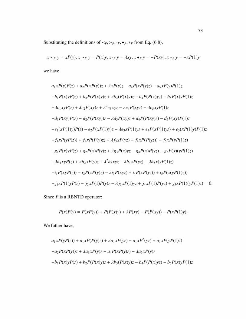
73

Substituting the definitions of ≺P,�P, ·P, •P, ∗P from Eq. (6.8),

x ≺P y = xP(y), x �P y = P(x)y, x ·P y = λxy, x •P y = −P(xy), x ∗P y = −xP(1)y

we have

a1xP(y)P(z) + a2P(xP(y))z + λxP(y)z − a4P(xP(y)z) − a5xP(y)P(1)z

+b1P(x)yP(z) + b2P(P(x)y)z + λb3(P(x)y)z − b4P(P(x)yz) − b5P(x)yP(1)z

+λc1xyP(z) + λc2P(xy)z + λ2c3xyz − λc4P(xyz) − λc5xyP(1)z

−d1P(xy)P(z) − d2P(P(xy))z − λd3P(xy)z + d4P(P(xy)z) − d5P(xy)P(1)z

+e1(xP(1)y)P(z) − e2P(xP(1)y)z − λe3xP(1)yz + e4P(xP(1)yz) + e5(xP(1)y)P(1)z

+ f1xP(yP(z)) + f2xP(P(y)z) + λ f3xP(yz) − f4xP(P(yz)) − f5xP(yP(1)z)

+g1P(x)yP(z) + g2P(x)P(y)z + λg3P(x)yz − g4P(x)P(yz) − g5P(x)(yP(1)z)

+λh1xyP(z) + λh2xP(y)z + λ2h3xyz − λh4xP(yz) − λh5x(yP(1)z)

−i1P(xyP(z)) − i2P(xP(y)z) − λi3P(xyz) + i4P(xP(yz)) + i5P(x(yP(1)z))

− j1xP(1)yP(z) − j2xP(1)P(y)z − λ j3xP(1)yz + j4xP(1)P(yz) + j5xP(1)(yP(1)z) = 0.

Since P is a RBNTD operator:

P(x)P(y) = P(xP(y)) + P(P(x)y) + λP(xy) − P(P(xy)) − P(xP(1)y).

We futher have,

a1xP(yP(z)) + a1xP(P(y)z) + λa1xP(yz) − a1xP2(yz) − a1xP(yP(1)z)

+a2P(xP(y))z + λa3xP(y)z − a4P(xP(y)z) − λa5xP(y)z

+b1P(x)yP(z) + b2P(P(x)y)z + λb3(P(x)y)z − b4P(P(x)yz) − b5P(x)yP(1)z

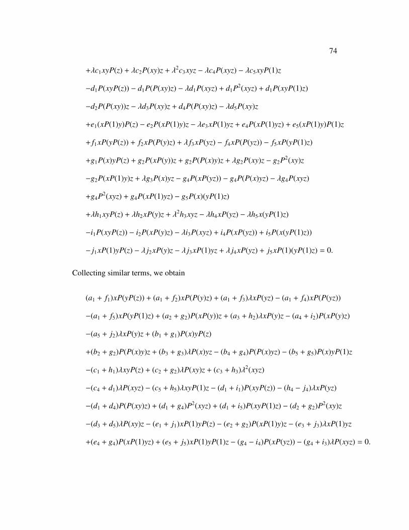
74

+λc1xyP(z) + λc2P(xy)z + λ2c3xyz − λc4P(xyz) − λc5xyP(1)z

−d1P(xyP(z)) − d1P(P(xy)z) − λd1P(xyz) + d1P2(xyz) + d1P(xyP(1)z)

−d2P(P(xy))z − λd3P(xy)z + d4P(P(xy)z) − λd5P(xy)z

+e1(xP(1)y)P(z) − e2P(xP(1)y)z − λe3xP(1)yz + e4P(xP(1)yz) + e5(xP(1)y)P(1)z

+ f1xP(yP(z)) + f2xP(P(y)z) + λ f3xP(yz) − f4xP(P(yz)) − f5xP(yP(1)z)

+g1P(x)yP(z) + g2P(xP(y))z + g2P(P(x)y)z + λg2P(xy)z − g2P2(xy)z

−g2P(xP(1)y)z + λg3P(x)yz − g4P(xP(yz)) − g4P(P(x)yz) − λg4P(xyz)

+g4P2(xyz) + g4P(xP(1)yz) − g5P(x)(yP(1)z)

+λh1xyP(z) + λh2xP(y)z + λ2h3xyz − λh4xP(yz) − λh5x(yP(1)z)

−i1P(xyP(z)) − i2P(xP(y)z) − λi3P(xyz) + i4P(xP(yz)) + i5P(x(yP(1)z))

− j1xP(1)yP(z) − λ j2xP(y)z − λ j3xP(1)yz + λ j4xP(yz) + j5xP(1)(yP(1)z) = 0.

Collecting similar terms, we obtain

(a1 + f1)xP(yP(z)) + (a1 + f2)xP(P(y)z) + (a1 + f3)λxP(yz) − (a1 + f4)xP(P(yz))

−(a1 + f5)xP(yP(1)z) + (a2 + g2)P(xP(y))z + (a3 + h2)λxP(y)z − (a4 + i2)P(xP(y)z)

−(a5 + j2)λxP(y)z + (b1 + g1)P(x)yP(z)

+(b2 + g2)P(P(x)y)z + (b3 + g3)λP(x)yz − (b4 + g4)P(P(x)yz) − (b5 + g5)P(x)yP(1)z

−(c1 + h1)λxyP(z) + (c2 + g2)λP(xy)z + (c3 + h3)λ2(xyz)

−(c4 + d1)λP(xyz) − (c5 + h5)λxyP(1)z − (d1 + i1)P(xyP(z)) − (h4 − j4)λxP(yz)

−(d1 + d4)P(P(xy)z) + (d1 + g4)P2(xyz) + (d1 + i5)P(xyP(1)z) − (d2 + g2)P2(xy)z

−(d3 + d5)λP(xy)z − (e1 + j1)xP(1)yP(z) − (e2 + g2)P(xP(1)y)z − (e3 + j3)λxP(1)yz

+(e4 + g4)P(xP(1)yz) + (e5 + j5)xP(1)yP(1)z − (g4 − i4)P(xP(yz)) − (g4 + i3)λP(xyz) = 0.

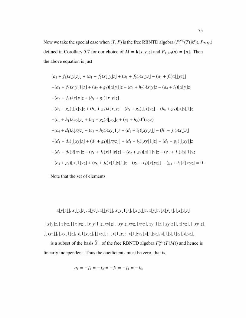
75

Now we take the special case when (T, P) is the free RBNTD algebra (FNCT (T (M)), PT (M))

defined in Corollary 5.7 for our choice of M = k{x, y, z} and PT (M)(u) = buc. Then

the above equation is just

(a1 + f1)xbybzcc + (a1 + f2)xbbyczc + (a1 + f3)λxbyzc − (a1 + f4)xbbyzcc

−(a1 + f5)xbyb1czc + (a2 + g2)bxbyccz + (a3 + h2)λxbycz − (a4 + i2)bxbyczc

−(a5 + j2)λxbycz + (b1 + g1)bxcybzc

+(b2 + g2)bbxcycz + (b3 + g3)λbxcyz − (b4 + g4)bbxcyzc − (b5 + g5)bxcyb1cz

−(c1 + h1)λxybzc + (c2 + g2)λbxycz + (c3 + h3)λ2(xyz)

−(c4 + d1)λbxyzc − (c5 + h5)λxyb1cz − (d1 + i1)bxybzcc − (h4 − j4)λxbyzc

−(d1 + d4)bbxyczc + (d1 + g4)bbxyzcc + (d1 + i5)bxyb1czc − (d2 + g2)bbxyccz

−(d3 + d5)λbxycz − (e1 + j1)xb1cybzc − (e2 + g2)bxb1cycz − (e3 + j3)λxb1cyz

+(e4 + g4)bxb1cyzc + (e5 + j5)xb1cyb1cz − (g4 − i4)bxbyzcc − (g4 + i3)λbxyzc = 0.

Note that the set of elements

xbybzcc, xbbyczc, xbyzc, xbbyzcc, xbyb1czc, bxbyccz, xbycz, bxbyczc, bxcybzc

bbxcycz, bxcyz, bbxcyzc, bxcyb1cz, xybzc, bxycz, xyz, bxyzc, xyb1cz, bxybzcc, xbyzc, bbxyczc,

bbxyzcc, bxyb1czc, xb1cybzc, bbxyccz, bxb1cycz, xb1cyz, bxb1cyzc, xb1cyb1cz, bxbyzcc

is a subset of the basis X∞ of the free RBNTD algebra FNCT (T (M)) and hence is

linearly independent. Thus the coefficients must be zero, that is,

a1 = − f1 = − f2 = − f3 = − f4 = − f5,

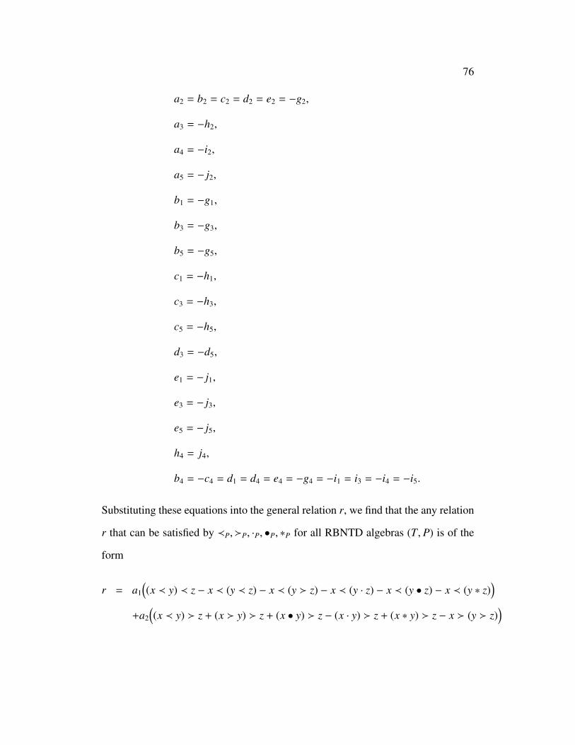
76

a2 = b2 = c2 = d2 = e2 = −g2,

a3 = −h2,

a4 = −i2,

a5 = − j2,

b1 = −g1,

b3 = −g3,

b5 = −g5,

c1 = −h1,

c3 = −h3,

c5 = −h5,

d3 = −d5,

e1 = − j1,

e3 = − j3,

e5 = − j5,

h4 = j4,

b4 = −c4 = d1 = d4 = e4 = −g4 = −i1 = i3 = −i4 = −i5.

Substituting these equations into the general relation r, we find that the any relation

r that can be satisfied by ≺P,�P, ·P, •P, ∗P for all RBNTD algebras (T, P) is of the

form

r = a1

((x ≺ y) ≺ z − x ≺ (y ≺ z) − x ≺ (y � z) − x ≺ (y · z) − x ≺ (y • z) − x ≺ (y ∗ z)

)+a2

((x ≺ y) � z + (x � y) � z + (x • y) � z − (x · y) � z + (x ∗ y) � z − x � (y � z)

)

77

+a3

((x ≺ y) · z − x · (y � z)

)+a4

((x ≺ y) • z − x • (y ≺ z)

)+a5

((x ≺ y) ∗ z − x ∗ (y � z)

)+b1

((x � y) ≺ z − x � (y ≺ z)

)+b3

((x � y) · z − x � (y · z)

)+b5

((x � y) ∗ z − x � (y ∗ z)

)+c1

((x · y) ≺ z − x · (y ≺ z)

)+c3

((x · y) · z − x · (y · z)

)+c5

((x · y) ∗ z − x · (y ∗ z)

)+d3

((x • y) · z − (x • y) ∗ z

)+e1

((x ∗ y) ≺ z − x ∗ (y ≺ z)

)+e3

((x ∗ y) · z − x ∗ (y · z)

)+e5

((x ∗ y) ∗ z − x ∗ (y ∗ z)

)+h4

(x · (y • z) + x ∗ (y • z)

)+b4

((x � y) • z − (x · y) • z + (x • y) ≺ z + (x • y) • z + (x ∗ y) • z

−x � (y • z) − x • (y ≺ z) + x • (y · z) − x • (y • z) − x • (y ∗ z)),

where a1, a2, a3, a4, a5, b1, b3, b4, b5, c1, c3, c5, d3, e1, e3, e5, h4 ∈ k can be arbitrary.

Thus r is in the subspace prescribed in Item 2, as needed.

(2⇒ 1) We check directly that all the relations in Eq. (6.13) are satisfied by (T,≺P

,�P, ·P, •P, ∗P) for every RBNTD algebra (T, P).

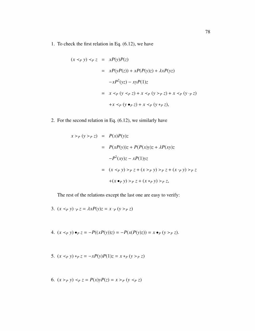
78

1. To check the first relation in Eq. (6.12), we have

(x ≺P y) ≺P z = xP(y)P(z)

= xP(yP(z)) + xP(P(y)z) + λxP(yz)

−xP2(yz) − xyP(1)z

= x ≺P (y ≺P z) + x ≺P (y �P z) + x ≺P (y ·P z)

+x ≺P (y •P z) + x ≺P (y ∗P z),

2. For the second relation in Eq. (6.12), we similarly have

x �P (y �P z) = P(x)P(y)z

= P(xP(y))z + P(P(x)y)z + λP(xy)z

−P2(xy)z − xP(1)yz

= (x ≺P y) �P z + (x �P y) �P z + (x ·P y) �P z

+(x •P y) �P z + (x ∗P y) �P z,

The rest of the relations except the last one are easy to verify:

3. (x ≺P y) ·P z = λxP(y)z = x ·P (y �P z)

4. (x ≺P y) •P z = −P((xP(y))z) = −P(x(P(y)z)) = x •P (y �P z).

5. (x ≺P y) ∗P z = −xP(y)P(1)z = x ∗P (y �P z)

6. (x �P y) ≺P z = P(x)yP(z) = x �P (y ≺P z)

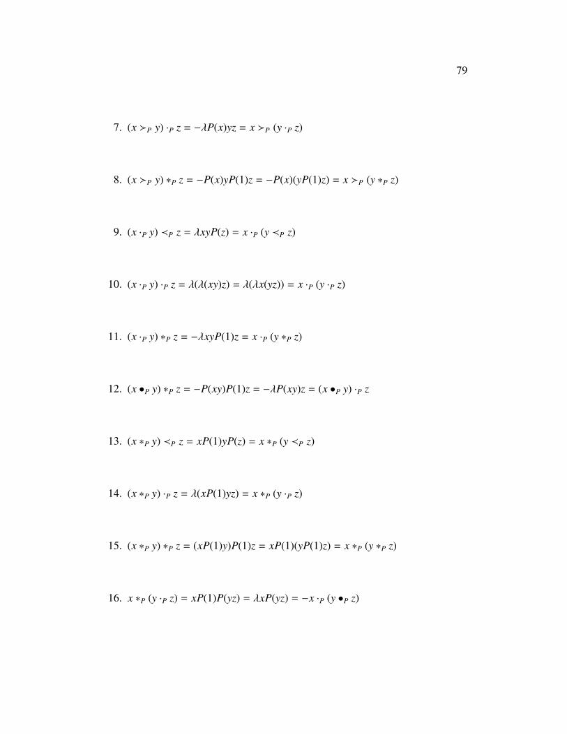
79

7. (x �P y) ·P z = −λP(x)yz = x �P (y ·P z)

8. (x �P y) ∗P z = −P(x)yP(1)z = −P(x)(yP(1)z) = x �P (y ∗P z)

9. (x ·P y) ≺P z = λxyP(z) = x ·P (y ≺P z)

10. (x ·P y) ·P z = λ(λ(xy)z) = λ(λx(yz)) = x ·P (y ·P z)

11. (x ·P y) ∗P z = −λxyP(1)z = x ·P (y ∗P z)

12. (x •P y) ∗P z = −P(xy)P(1)z = −λP(xy)z = (x •P y) ·P z

13. (x ∗P y) ≺P z = xP(1)yP(z) = x ∗P (y ≺P z)

14. (x ∗P y) ·P z = λ(xP(1)yz) = x ∗P (y ·P z)

15. (x ∗P y) ∗P z = (xP(1)y)P(1)z = xP(1)(yP(1)z) = x ∗P (y ∗P z)

16. x ∗P (y ·P z) = xP(1)P(yz) = λxP(yz) = −x ·P (y •P z)

80

17. For the last relation in Eq. (6.12), we check that the left hand side is

(x �P y) •P z + (x •P y) ≺P z + (x •P y) •P z − (x ·P y) •P z + (x ∗P y) •P z

= −P((P(x)y)z) − P(xy)P(z) + P(P(xy)z) + λP(xyz) + P(xP(1)yz)

= −P(P(x)yz) − P(xyP(z)) − P(P(xy)z) + P2(xyz) − λP(xyz) + P(xyP(1)z)

+P(P(xy)z) + λP(xyz) + P(xP(1)yz)

= −P(P(x)yz) − P(xyP(z)) + P2(xyz) + P(xyP(1)z) + P(xP(1)yz),

which agrees with the right hand side

x �P (y •P z) + x •P (y ≺P z) + x •P (y •P z) − x •P (y ·P z) + x •P (y ∗P z)

= −P(x)P(yz) − P(x(yP(z))) + P(xP(yz)) + P(x(λyz)) + P(x(yP(1)z))

= −P(xP(yz)) − P(P(x)yz) + P2(xyz) − λP(xyz) + P(xP(1)yz) − P(x(yP(z)))

+P(xP(yz)) + λP(xyz) + P(x(yP(1)z))

= −P(P(x)yz) + P2(xyz) − P(xyP(z)) + P(xP(1)yz) + P(x(yP(1)z)).

Thus, if the relation space R of an operadP = P(V)/(R) is contained in the subspace

spanned by the vectors in Eq. (6.12), then the corresponding relations are linear

combinations of the equations in Eq. (6.13) and hence are satisfied by (T,≺P,�P

, ·P, •P, ∗P) for each RBNTD algebra (T, P). Therefore (T,≺P,�P, ·P, •P, ∗P) is a

P-algebra. This completes the proof of Theorem 6.6

81

References

[1] Aguiar, M. Infinitesimal hopf algebras. Contemporary Mathematics, 267

(2000), 1–29.

[2] Aguiar, M. Prepoison algebras. Lett. Math. Phys., 54 (2000), 263–277.

[3] Andrews, G. E., Guo, L., Keigher, W., and Ono, K. Baxter algebras and hopf

algebras. Trans. AMS, 355 (2003), 4639–4656.

[4] Bai, C., Guo, L., and Zhang, Y. Totally compatible algebras and lie algebras,

rota-baxter operators and postlie algebras. Sci. China Math., 57 (2014), 259–

273.

[5] Baxter, G. An analytic problem whose solution follows from a simple alge-

braic identity. Pacific J. Math., 10 (1960), 731–742.

[6] Carinena, J., Grabowski, J., and Marmo, G. Quantum bi-hamiltonian systems.

Internat. J. Modern Phys. A, 15 (2000), 4797–4810.

[7] Cartier, P. On the structure of free baxter algebras. Adv. in Math., 9 (1972),

253–265.

[8] Connes, A., and Kreimer, D. Renormalization in quantum field theory and the

riemann-hilbert problem. i. the hopf algebra structure of graphs and the main

theorem. Comm. Math. Phys. 1, 210 (2000), 249–273.

[9] Connes, A., and Kreimer, D. Renormalization in quantum field theory and the

riemann-hilbert problem. ii. the β -function, diffeomorphisms and the renor-

malization group. Comm. Math. Phys. 1, 216 (2001), 215–241.

82

[10] Ebrahimi-Fard, K. Loday-type algebras and the rota-baxter relation. Lett.

Math. Phys., 61 (2002), 139–147.

[11] Ebrahimi-Fard, K., and Guo, L. Quasi-shuffles, mixable shuffles and hopf

algebras. J. Algebraic Combin., 24 (2006), 83–101.

[12] Ebrahimi-Fard, K., and Guo, L. Free rota-baxter algebras and rooted trees. J.

Algebra and Its Applications, 7 (2008), 167–194.

[13] Ebrahimi-Fard, K., and Guo, L. Rota-baxter algebras and dendriform alge-

bras. Jour. Pure Appl. Algebra, 212 (2008), 320–339.

[14] Ebrahimi-Fard, K., Guo, L., and Kreimer, D. Spitzer’s identity and the al-

gebraic birkhoff decomposition in pqft. J. Phys. A: Math. Gen., 37 (2004),

11037–11052.

[15] Ebrahimi-Fard, K., Guo, L., and Kreimer, D. Integrable renormalization ii:the

general case. Annales Henri Poincare, 6 (2005), 369–395.

[16] Ebrahimi-Fard, K., and Leroux, P. Generalized shuffles related to nijenhuis

and td-algebras. Comm. Algebra, 37 (2009), 3065–3094.

[17] Frolicher, A., and Nijenhuis, A. Theory of vector valued differential forms.

part i. Indag. Math., 18 (1956), 338–360.

[18] Golubchik, I. Z., and Sokolov, V. V. Generalized operator yang-baxter equa-

tions, integrable odes and nonassociative algebras. J. of Nonlinear Math.

Phys., 7 (2000), 184–197.

83

[19] Golubchik, I. Z., and Sokolov, V. V. One more type of classical yang-baxter

equation. Funct. Anal. Appl., 34 (2000), 296–298.

[20] Guo, L. Baxter algebras and the umbral calculus. Adv. in Appl. Math., 27

(2001), 405–426.

[21] Guo, L. An Introduction to Rota-Baxter Algebras. Higher Education Press

(China) and International Press (US), 2010.

[22] Guo, L., and Keigher, W. Baxter algebras and shuffle products. Adv. Math.,

150 (2000), 117–149.

[23] Guo, L., and Lei, P. Nijenhuis algebras, ns algebras and n-dendriform algebra.

Front. Math. China, 7 (2012), 827–846.

[24] Guo, L., Sit, W. Y., and Zhang, R. On rota’s problem for linear operators in

associative algebras. Proceedings ISSAC 2011 (2011), 147–154.

[25] Hoffman, M. E. The algebra of multiple harmonic series. J. Algebra, 194

(1997), 477–495.

[26] Leroux, P. Construction of nijenhuis operators and dendriform trialgebras. Int.

J. Math. Math. Sci. 40-52 (2004), 2595–2615.

[27] Loday, J. L. Une version non commutative des algebremde lie:les algberes de

leibniz. Ens. Math., 39 (1993), 269–293.

[28] Loday, J. L. Dialgebras. Dialgebras and related operads, 1763 (2001), 7–66.

84

[29] Loday, J. L., and Ronco, M. Trialgebras and families of polytopes, in ho-

motopy theory: Relations with algebraic geometry, group cohomology, and

algebraic k-theory”. Contemp. Math., 346 (2004), 369–398.

[30] Loday, J. L., and Vallette, B. Algebraic Operads. No. 346. Springer, Heidel-

berg, 2012.

[31] Nijenhuis, A. xn−1-forming sets of eigenvectors. Indag. Math., 13 (1951),

200–212.

[32] Rota, G. Baxter algebras and combinatorial identities i. Bulletin of the Amer-

ican Mathematical Society 75, 2 (1975), 325–329.

[33] Rota, G. Baxter operators, an introduction. Gian-Rota Rota on Combinatorics,

Introductory papers and commentaries, Birkhauser, Boston (1995), 504–512.

[34] Uchino, K. Twisting on associative algebras and rota-baxter type operators. J.

Noncommut. Geom., 4 (2010), 349–379.

[35] Zhou, C. Free TD-algebras. World Scientific Publishing Company, 2012.

85

Curriculum Vitae

1981 Born March 30th in Chandigarh, India.

1998-2003 Attended Department of Mathematics,

Panjab University,Chandigarh,India

2003 M.Sc (Hons School) Mathematics,

Panjab University,Chandigarh,India.

2008-14 Graduate work in Mathematics, Rutgers University,

Newark, New Jersey,USA.

2008-13 Teaching Assistantship, Department of Mathematics

and Computer Science at Rutgers-Newark,USA.

2013-14 Dissertation Fellowship, Rutgers University-Newark,USA.

2014 Ph.D. in Mathematical Sciences.

on rota-baxter nijenhuis td algebra

Documents