on reactive power compensation of wind farms – impact of wind farm

1

ON REACTIVE POWER COMPENSATION OF WIND FARMS –

IMPACTOFWINDFARMCONTROLLERDELAYS

Master of Science Thesis in Electrical Power Engineering

ARSLAN ASHRAF

Department of Energy and Environment Division of Electric Power Engineering

CHALMERS UNIVERSITY OF TECHNOLOGY Göteborg, Sweden 2011

Master’s Thesis xxxxxx

2

MASTER’S THESIS XXXXXXX

ONREACTIVEPOWERCOMPENSATIONOFWINDFARMS–

IMPACTOFWINDFARMCONTROLLERDELAYS

Master of Science Thesis in Electric Power Engineering

ARSLAN ASHRAF

Department of Energy and Environment Division of Electric Power Engineering

CHALMERS UNIVERSITY OF TECHNOLOGY Göteborg, Sweden 2011

3

On Reactive Power Compensation of Wind Farms – Impact of Wind Farm Controller Delays

Master of Science Thesis in Electric Power Engineering

ARSLAN ASHRAF

© ARSLAN ASHRAF, 2011

Master’s Thesis XXXXXX ISSN XXXX-XXXX Department of Energy and Environment

Division of Electric Power Engineering

Chalmers University of Technology

SE-412 96 Göteborg

Sweden

Telephone: + 46 (0)31-772 1000

4

ACKNOWLEDGEMENTS:

I would like to pay my deepest gratitude to my examiner and main supervisor, Assoc. Prof. Massimo Bongiorno, for his technical guidance, fruitful discussions, support and patience. I would like to sincerely thank Dr. Tarik Abdulahovic, Electric Power Engineering, and Sr. Research Engineer Aleksander Bartnicki, High Voltage Engineering, for their guidance, help and support regarding the section of cables.

I would like to thank PhD student, Faisal Altaf, Department of Signals and Systems, for his valuable time and nice discussions.

I am grateful to all the staff members of Electric Power Engineering and High Voltage Engineering departments for grooming me with knowledge, and providing the nice and friendly environment during my stay at Chalmers.

I further share my gratitude to Jan-Olov Lantto and Valborg Ekman for their assistance and support.

Thanks to all my fellow Masters students who have assisted me in several ways. In particular, I will like to thank Abdul Basit, Waqas Baig, Mattias Persson, Syed Sagheer Hussain Shah Jillani and Muhammad Adnan Azmat for all their support and help.

I would also like to thank my friends Mian Imran Hussain and Amin ur Rehman Khan for their moral support and encouragement. Thanks to my parents, Mrs. Aqeela and Mr. Ashraf, my wife, Shamsa, my sister, Najaf, and my brother, Burhan, for their love, encouragement and support. Last, but surely not the least, I would like to thank my daughter, Tajweed, for her love which I will always cherish. Arslan Ashraf Gothenburg, Sweden June, 2012

5

ABSTRACT:

In the past few decades, Wind energy has proved to be a fastest growing renewable energy source globally and its large scale penetration in the interconnected systems is consistently imposing new challenges for the engineers. Attending to the technological advancements and the upgrading requirements of the power companies a proper control scheme for the reactive power compensation in a wind farm is necessary. The control architecture constitutes of a supervisory control system which bridges different parts of the wind farm in order to calculate and regulate the reactive power compensation from each wind turbine. This complete process of data acquisition, calculation and regulation enforces a time delay which impacts the system dynamics and behavior. This thesis focuses on the understanding of the influence of this time delay on the dynamic performance of the overall system during reactive power compensation operation.

6

Contents

1. INTRODUCTION....................................................................................................... 9

1.1. BACKGROUND .................................................................................................. 9

1.2. PURPOSE OF STUDY ....................................................................................... 9

1.3. OUTLINE OF THE THESIS .............................................................................. 11

2. WIND ENERGY-GENERATION SYSTEMS ........................................................... 12

2.1. INTRODUCTION .............................................................................................. 12

2.2. WIND TURBINE ARCHITECTURES ................................................................ 12

2.2.1. FIXED SPEED TURBINES ........................................................................ 12

2.2.2. VARIABLE SPEED TURBINES ................................................................. 13

2.3. WIND PARKS VERSUS CONVENTIONAL POWER PLANTS ........................ 14

2.3.3. LOCAL IMPACTS ...................................................................................... 15

2.3.4. SYSTEM-WIDE IMPACTS ......................................................................... 15

2.4. CONCLUSION.................................................................................................. 15

3. FULL POWER CONVERTER BASED WIND TURBINES ....................................... 17

3.1. INTRODUCTION .............................................................................................. 17

3.2. FULLY RATED CONVERTERS ....................................................................... 17

3.3. GRID CONNECTED VOLTAGE SOURCE CONVERTER ............................... 19

3.3.1. MODULATION TECHNIQUES ................................................................... 19

3.3.2. SWITCHING FREQUENCY ....................................................................... 19

3.4. GRID INTEGRATION ....................................................................................... 20

3.4.1. THE SYSTEM PARAMETERS .................................................................. 21

3.4.2. THE DC LINK VOLTAGE ........................................................................... 21

3.4.3. THE FILTER .............................................................................................. 22

3.4.4. THE TRANSFORMER ............................................................................... 22

3.4.5. THE TRANSMISSION CABLE ................................................................... 23

3.4.6. THE GRID .................................................................................................. 23

3.4.7. PSCAD MODELING .................................................................................. 24

3.5. CABLE RESONANCE ...................................................................................... 24

3.6. CONTROL ACTION ......................................................................................... 25

3.6.1. COMMON GRID CODES ........................................................................... 25

7

3.6.2. ADVANCED GRID OPERATION ............................................................... 28

3.7. CONCLUSION.................................................................................................. 29

4. CONTROL DESIGN FOR REACTIVE POWER COMPENSATION ........................ 30

4.1. INTRODUCTION .............................................................................................. 30

4.2. CONTROL METHOD ....................................................................................... 30

4.3. PLL ESTIMATOR ............................................................................................. 31

4.4. CURRENT CONTROLLER .............................................................................. 34

4.5. ACTIVE POWER CONTROLLER ..................................................................... 37

4.6. REACTIVE POWER CONTROL....................................................................... 39

4.6.1. REACTIVE POWER CONTROLLER ......................................................... 39

4.6.2. VOLTAGE CONTROLLER......................................................................... 40

4.7. SATURATION AND INTEGRATION ANTI-WINDUP ........................................ 42

4.7.1. INNER CONTROLLER .............................................................................. 42

4.7.2. OUTER CONTROLLER ............................................................................. 44

4.8. VOLTAGE SUPPORT ALGORITHM ................................................................ 45

4.9. ACTIVE POWER REFERENCE ....................................................................... 46

4.10. TIME DELAY ................................................................................................. 46

4.11. CONCLUSION .............................................................................................. 46

5. RESULTS AND SIMULATION ................................................................................ 48

5.1. INTRODUCTION .............................................................................................. 48

5.2. RESULTS WITH CONVENTIONAL VOLTAGE CONTROLLER ...................... 49

5.2.1. USING Zcable AND NO TIME DELAY ......................................................... 49

5.2.2. WITH TRANSMISSION CABLES AND NO TIME DELAY ......................... 55

5.2.3. USING Zcable WITH 50ms TIME DELAY ..................................................... 64

5.2.4. WITH TRANSMISSION CABLE AND 50ms TIME DELAY ........................ 70

5.2.5. WITH Zcable AND 100ms TIME DELAY ....................................................... 73

5.2.6. WITH TRANSMISSION CABLE AND 100ms TIME DELAY ...................... 76

5.3. SIMULATION RESULTS WITH VOLTAGE SUPPORT ALGORITHM .............. 78

5.3.1. WITH Zcable AND NO TIME DELAYS ......................................................... 78

5.3.2. WITH TRANSMISSION CABLE AND NO TIME DELAY ............................ 84

5.3.3. WITH Zcable AND 100ms TIME DELAY ................................................... 86

8


5.3.5. WITH Zcable AND 200ms TIME DELAY ................................................... 91


5.4. CONCLUSION.................................................................................................. 96

6. CONCLUSION AND FUTURE WORK .................................................................... 97

APPENDIX-A: TRANSFORMER DATA ......................................................................... 99

APPENDIX-B: TRANSMISSION CABLE DATA .......................................................... 100

APPENDIX-C: TRANSFORMATIONS ......................................................................... 109

7. BIBLIOGRAPHY ................................................................................................... 111

9

1. INTRODUCTION

1.1. BACKGROUND

The world’s energy resources are not sufficient to sustain expected growth trends. A growing gap is developing between energy demand and the available supply of oil and gas. High energy prices are expected to stay and the world’s energy mix is visualized to change[1].

Also, there is a general acceptance that burning of fossil fuels is playing a significant role in the global climatic changes. Effective mitigation of the climatic change requires a huge reduction in the greenhouse gas emissions. The electricity systems are considered to be easily transferable to low carbon energy sources compared to the other sectors like domestic heating and air transport etc. Hence, the use of cost effective and reliable low carbon electricity generation sources is becoming a vital objective of energy policy in many countries.

Wind energy has shown the fastest growth rate of any form of electricity generation with its development simulated by the concerns of climate change, energy diversity and security of supply in past few decades. Owing to ongoing improvements in turbine efficiency and higher fuel prices, wind power is becoming economically competitive with conventional power production, and at sites with high wind speeds on land, wind power is considered to be fully viable. GWEC predicts that at the end of 2015, global wind capacity will stand at 459GW, up from 197GW at the end of 2010[2].

This large scale penetration of wind energy in the electrical network systems is consistently imposing challenges to the engineers due to the proportionate advancement of technology and provides an increasing evidence of the influence between wind farms and the grid.

1.2. PURPOSE OF STUDY

Advancements in the technology of power electronics have developed interest in large capacity variable-speed wind turbines in the MW range. Today large-scale integration of wind sources into the grid via full-power converters is being increasingly adapted due to its high power density and controllability.

With variable-speed wind turbines, the sensitivity of the power electronics to over-currents caused by network voltage depressions can have serious consequences for the stability of the power system. Also, the considerable amount of wind energy generated and delivered to the interconnected electrical network significantly depends on the wind conditions, which evidently raises a risk factor for the balance between energy offer and

10

demand. Thus, to avoid reliability issues and network stability problems, grid operators launch guidelines for net connection of wind turbines.

In some countries, the wind farm can also be used to stabilize the grid providing reactive power compensation. This feature becomes of particular interest in case of wind farms connected to weak grids and is achieved by proper control algorithms in a wind farm.

Operators of the wind farms should be able to monitor and control the status and operating conditions of each turbine as well as the combined electrical response of the wind farm, keeping in view the grid interconnection requirements. It is therefore highly necessary to measure and monitor the point of connection of the wind farm to the grid as well as each individual turbine. Thus, the control system of each individual turbine should be connected to a supervision system that supervises the operation situation and power regulation of the whole wind farm. This supervision system also fetches operation data from grid regulation system of the whole wind farm and reactive power requirements. A general topology of such a control system of a wind farm comprising of Full Power Converter wind turbines is shown in Figure 1.1.

Figure 1.1: General topology of Wind Farm Reactive Power Control System

11

The process of data acquisition from grid regulation system to the wind farm reactive power adjustment to the desired level enforces a time delay which has an impact on the overall system behavior and acquires the attention of control engineers and researchers.

The main objective of this thesis is to design and investigate a supervisory control system for reactive power compensation provided by the wind farm. Of particular interest will be to investigate the influence of the delay on the system dynamics and behavior arising from acquisition of information from the grid regulation system through to the ultimate response of the wind farm to control the reactive power.

The key milestones of the project are:

• Study of the control strategies and performance evaluation of the Full Power Converter wind turbines.

• Selection of an appropriate control topology of the grid side converter of a back to back full power converter to attain the desired results.

• Designing of control system in PSCAD to study, real time performance of the Wind Farm.

• Investigate the impact of time delay generated as a result of data acquisition on the operation of the grid connected wind farm under normal and fault conditions.

1.3. OUTLINE OF THE THESIS

Chapter 2 briefly overviews the commonly used wind turbine configurations and compares the wind energy conversion systems to the conventional power plants.

Chapter 3 introduces to the fully rated power converter based wind farms and covers the mathematical analysis of the active and reactive power with calculation of their theoretical limits.

Chapter 4 presents the modeling of reactive power compensation of individual FRC wind turbines and explains the basic components of the control scheme.

Chapter 5 introduces the operational working of the control system designed for reactive power compensation at the point of common connection and presents the characteristics of the system when time delays exist within the system.

Chapter 6 briefly overviews the findings and ends up by giving the future prospects to be considered in this context.

12

2. WIND ENERGY-GENERATION SYSTEMS

2.1. INTRODUCTION

Utilization of the wind energy has been a historic concept. In the beginning of twentieth century wind energy was used for electric power generation for the first time but the idea never received attention until 1970. Since then, step by step developments have made wind power generation an important part of the power systems.

A standard wind turbine plant of today uses horizontal axis configuration. A horizontal axis wind turbine consists of a tower and a nacelle mounted on the top of the tower. The nacelle usually comprises of the generator, gearbox and the rotor. The rotor has a different number of blades depending on the application of the wind turbine. Two bladed and three bladed rotors are used for the electric power generation application[3]. Currently, three bladed wind turbines dominate the market due to lower aerodynamic noise and blade drag losses.

However, these wind power conversion systems behave different, in comparison to the conventional power plants, when connected to the grid. A lot of effort is being delivered by the researchers and engineers to attain the dynamic behavior of wind power plants as that of conventional power plants.

In this chapter we will discuss the modern wind power plants and then briefly compare the wind power plants with that of the conventional power plants.

2.2. WIND TURBINE ARCHITECTURES

Wind Turbines are classified according to their drive train as follows:

2.2.1. FIXED SPEED TURBINES

Fixed-speed wind turbines are designed to achieve maximum efficiency at a particular speed. This implies that regardless of the wind speed, the rotor speed is fixed and determined by the gear ratio, generator design and the grid frequency[4]. These devices consist of an induction generator connected directly to the grid as shown in Figure 2.1. It must be mentioned here that as induction machines consume reactive power, and produce high transient currents while energizing, an installation of compensation capacitors along with soft starter unit is necessary.

Fixed speed wind turbines are considered to be simple, robust, reliable and cheap devices. However, limited power quality control, uncontrollable reactive power consumption and mechanical stress are the disadvantages of fixed speed wind turbines.

13

Gear Box

Transformer

Pout, Qout

Soft starterGridGenerator

Capacitor banks

IG

Figure 2.1: Fixed Speed Wind Turbine

2.2.2. VARIABLE SPEED TURBINES

Variable speed wind turbines are designed to obtain maximum efficiency over a wide range of wind speeds. These devices keep the generator torque to a constant level and the variations in the wind speed are absorbed by the changes in the generator speed. They are typically equipped with an induction or a synchronous generator and connected to the grid via power electronic interface [4].

The advantages of variable speed wind turbines are increased energy capture, improved power quality and lower mechanical stress. The disadvantages are complex structure, losses in power electronics and a higher cost.

Currently the most popular variable-speed wind turbine configurations are as follows:

Doubly Fed Induction Generator (DFIG) Wind Turbine

A typical configuration of a DFIG wind turbine is shown schematically in Figure 2.2. It uses a Wound Rotor Induction Generator (WRIG) with slip rings to take current into or out of the rotor winding and variable-speed operation is obtained by injecting a controllable voltage into the rotor at slip frequency [5].

Figure 2.2: General topology of a DFIG wind turbine

14

The rotor winding is fed through a variable-frequency power converter, typically based on two AC/DC IGBT-based voltage source converters (VSC) linked by a DC bus. The power converter decouples the network electrical frequency from the rotor mechanical frequency, enabling variable-speed operation of the wind turbine. The generator and converters are protected by voltage limits and an over-current ‘crowbar’.

A DFIG system can deliver power to the grid through the stator and rotor, while the rotor can also absorb power, depending on the rotational speed of the generator.

Fully Rated Converter (FRC) Wind Turbine

The typical configuration of a fully rated converter wind turbine is shown in Figure 2.3. A wide range of electrical generator types, for example, wound-rotor synchronous (WRSG) or permanent magnet synchronous (PMSG), can be employed in this type of turbines. In this configuration, all the power produced by the wind turbines is transferred through the power converters; therefore, the dynamic operation of the electrical generator is effectively isolated from the power grid[5]. In other words, the electrical frequency of the generator is independent of the grid frequency, thus allowing a variable-speed operation of the wind turbine.

Figure 2.3: General topology of a FRC wind turbine

Fully Rated Converter Wind Turbine is the main focus of this thesis and will be discussed later in detail.

2.3. WIND PARKS VERSUS CONVENTIONAL POWER PLANTS

There are significant differences between wind power and conventional synchronous central generation [6]:

• Wind turbines employ different, often converter-based, generating systems compared with those used in conventional power plants.

• The prime mover of wind turbines, the wind, is not controllable and fluctuates stochastically.

• The typical size of individual wind turbines is much smaller than that of a conventional utility synchronous generator.

15

Due to these differences, wind generation interacts differently with the network and wind generation may have both local and system-wide impacts on the operation of the power system.

2.3.3. LOCAL IMPACTS

Local impacts occur within the electrical vicinity of a wind turbine or wind farm, and can be attributed to a specific turbine or farm. These impacts can be listed as follows:

• Circuit power flows and bus-bar voltages • Protection schemes, fault currents, and switchgear rating • Power quality

Harmonic voltage distortion Voltage flicker.

The first two topics are always investigated during the installation of new generators and are not specific to wind power. Harmonic voltage distortion is of interest when power electronic converters are employed to interface wind generation units to the network whereas voltage flicker is more significant for large, fixed-speed wind turbines on weak distribution circuits.

2.3.4. SYSTEM-WIDE IMPACTS

System-wide impacts affect the behavior of the power system as a whole. They are an inherent consequence of the utilization of wind power and affect the following [6]:

• Power system dynamics and stability • Reactive power and voltage support • Frequency support.

The impact on power system dynamics and stability is due to the fact that a wind power generating units are not based on conventional synchronous generators. The wind turbines are installed at the locations with good wind profile and may not be favorable from the perspective of grid voltage control, thus, the impact on reactive power and voltage support is imminent. The impact of wind power on the frequency support or system balancing is caused by the fact that wind cannot be controlled. As a result, the wind power cannot contribute to the primary frequency regulation.

2.4. CONCLUSION

In this chapter the basic architectural classification of wind turbines was discussed. In this account it was presented that the fixed speed wind turbines are dominated by variable speed wind turbines due to their operation over a wide range of speed. Due to the availability of power electronics and better controllability, DFIG and FRC wind turbines are the most popular variable speed wind turbines. It was presented that due to this power electronic interface, uncontrollable nature of wind and small power ratings,

16

the wind power plants do not behave like conventional power plants in power systems. These differences as a consequence affect the system stability, dynamic performance, voltage and reactive power support, and frequency support.

Fully rated converter wind turbines will be discussed in the next chapter and the reactive power and voltage support being the main focus of the thesis will be analyzed later.

17

3. FULL POWER CONVERTER BASED WIND TURBINES

3.1. INTRODUCTION

Increasing penetration level of wind turbines has made it necessary to consider them while determining the stability of the grid [7]. The modern wind turbines are required to act as active controllable devices in the power systems. Thus, they are expected to meet higher technical demands, provided by the grid operators, like voltage regulation, active and reactive power control and to provide quick responses during transient and dynamic disturbances in the power system [4]. Owing to these requirements, fully rated converter based wind turbines are becoming popular, as they fully decouple the generator from the grid and provide complete controllability over the power flow [7].

3.2. FULLY RATED CONVERTERS

During past few years multiple topologies of frequency converters like back to back converters, multilevel converters and matrix converters etc. have been explored for the application of wind turbines. However, back to back fully rated converter is the most widely employed topology today [4].

The variable speed wind turbines based on these converters have three main components; the generator, the rectifier and the inverter. Also, they can be split into two main subsystems; the inverter-grid subsystem and the rectifier-generator subsystem [8]. Each subsystem can have at least two different device alternatives.

The generator can be either an induction generator or a synchronous generator. The synchronous generators that can be employed are[8]:

• Permanent Magnet Synchronous Generators (PMSG) • Wound Rotor Synchronous Generators (WRSG) • Switched Reluctance Synchronous Generators (SRSG)

The electrically excited generators when connected to the grid provide an advantage of controllable three phase voltage level [8]. However, due to the bulky construction and higher losses in rotor windings, PMSGs are becoming more popular [5]. Also, lower the efficiency and lower the power density of SRSGs makes PMSGs a better choice [4].

The generator can be interfaced to either a load commutated rectifier, i.e. a diode or a thyristor rectifier, or to a VSC. This choice of rectifier however is strictly restricted to the generator type i.e. synchronous or induction. The induction generators (IG) are usually connected to the VSC based rectifiers as these generators need reactive power for their operation and VSCs can produce it. However, the synchronous generators can be interfaced with any of the mentioned rectifiers [8]. The inverter of the back to back

18

converter is connected to the grid. Here again a grid commutated thyristor based inverter or a VSC can be employed.

Thyristor inverters have lower losses and, as they have been available for a wide range of power level for a while, have a lower cost. However, unlike thyristor inverters, the privilege of operating at almost unity power factor and ability to eliminate low frequency current harmonics, VSCs are becoming more popular in the commercial market [8].

In this arrangement, the generator side converter is usually responsible for the control of the generator speed in order to achieve Maximum Power Point Tracking and to set suitable magnetization demand (only in case of electrically excited generator installation). The DC link capacitor decouples the control of the two converters while, the grid side converter controls the power flow to the grid and regulates the dc link voltage [4].

Usually for wind turbine applications back to back two level converters comprising of two pulse width modulated (PWM) VSCs capable of bidirectional power flow as shown in Figure 3.1 are used. The valves of voltage source converters are generally considered to be of Insulated Gate Bipolar Transistor (IGBT) type.

Figure 3.1: Back to back two level converter topology

From the description of the thesis expressed in chapter 1 and the discussion above it should be mentioned here that as the focus of this thesis is on the reactive power control of a wind turbine, therefore we will only consider the control of a VSC connected to the grid. This implies that the type, operation and control of the generator or the generator side rectifier will not be considered and will be replaced by an ideal fixed DC source attached to the DC link.

19

3.3. GRID CONNECTED VOLTAGE SOURCE CONVERTER

Grid side VSC is a DC to AC converter consisting of three legs, one for each phase as shown Figure 3.1. Each leg consists of two valves. The switching of the valves is carried out in such a way that the fundamental of the output voltage is a three phase AC voltage of desired frequency and amplitude.

3.3.1. MODULATION TECHNIQUES

The main aim of the modulation techniques is to eliminate the low frequency harmonics and to ensure the output voltage is equal to the reference voltage waveform.

The switching pattern for the valves is determined by modulation techniques like Pulse Width Modulation (PWM), Space Vector Modulation (SVM) or Six-Pulse Method. The Six-Pulse modulation technique provides minimum switching frequency and is considered in large converters where the switching losses should be minimized. The PWM and SVM techniques, on the contrary, are used when lower conduction losses are of concern.

PWM is the classical modulation technique in which the three phase reference voltage waveforms are compared to a triangular carrier wave in order to generate the switching pattern. The intersection of each phase of the reference voltage with the carrier wave generates a switching pattern for the concerned leg of the VSC.

The six-pulse modulation is the simplest modulation technique in which each phase switches twice per cycle. The amplitude of the output fundamental voltage increases however low frequency harmonics are introduced [8][9]. In order to eliminate low frequency harmonics the switching frequency should be increased. The increase in the switching frequency reduces the current ripple which in turn pushes the harmonics to higher frequencies. However, the maximum amplitude of the output fundamental voltage is also reduced[8]. It should be noted here, that the privilege to operate at high switching frequencies is not provided by the six-pulse modulation.

In SVM the reference voltage vector is approximated by a time sequence of three well-defined switching state vectors [8]. This technique ensures that the time average of the switching state vectors over a sampling inverter is equal to the reference voltage.

PWM is the most popular technique due to its simple implementation and will be the focus for further discussions.

3.3.2. SWITCHING FREQUENCY

If the switches are considered to be ideal then there is no limit to the maximum choice of the switching frequency. However, in reality this is not achievable. The switching frequency fsw is considered to be higher than the desired fundamental frequency f1 of the output voltage and is given as [9]:

20

Where, mf is an integer referred as the frequency modulation ratio. Therefore, the minimum switching frequency which can be achieved is twice the desired fundamental frequency. The choice of mf is critical to harmonics introduced, therefore, mf is usually chosen as an odd integer, to eliminate the even harmonics, and a multiple of 3 in order to eliminate the most dominant 3rd harmonic and its multiples like 9th, 15th etc.[9].

On the contrary the choice of the switching frequency is also limited by rated power of the VSC. The switching losses increase proportionally to the switching frequency, which restricts the usage of higher switching frequency when the rated power of the system is increased. Therefore, for high power applications, the choice of switching frequency is reduced down to 2 kHz or less[9].

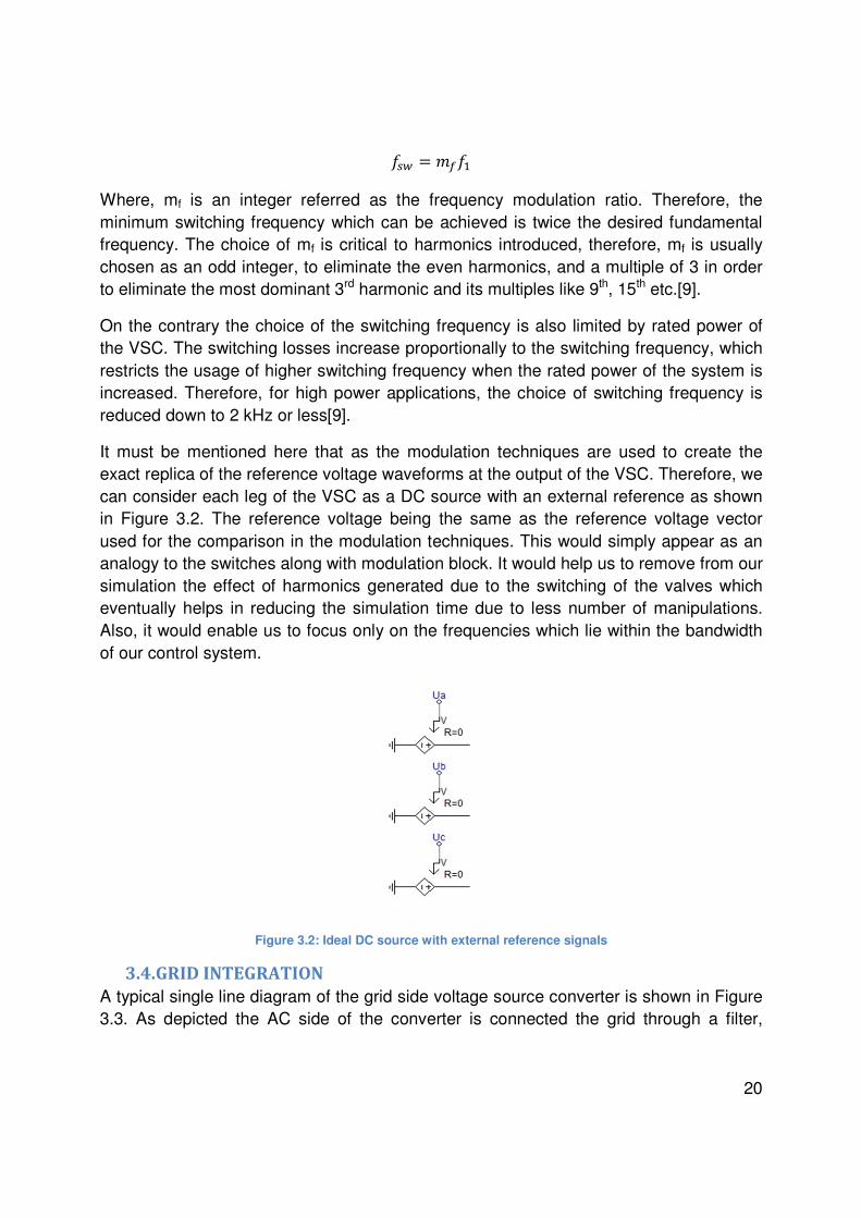
It must be mentioned here that as the modulation techniques are used to create the exact replica of the reference voltage waveforms at the output of the VSC. Therefore, we can consider each leg of the VSC as a DC source with an external reference as shown in Figure 3.2. The reference voltage being the same as the reference voltage vector used for the comparison in the modulation techniques. This would simply appear as an analogy to the switches along with modulation block. It would help us to remove from our simulation the effect of harmonics generated due to the switching of the valves which eventually helps in reducing the simulation time due to less number of manipulations. Also, it would enable us to focus only on the frequencies which lie within the bandwidth of our control system.

Figure 3.2: Ideal DC source with external reference signals

3.4. GRID INTEGRATION

A typical single line diagram of the grid side voltage source converter is shown in Figure 3.3. As depicted the AC side of the converter is connected the grid through a filter,

21

transformer, Transmission media (either cable or an overhead line) and short circuit impedance of the grid.

Figure 3.3: Single Line Diagram of the system implemented

3.4.1. THE SYSTEM PARAMETERS

The system base values chosen for the analysis are as follows:

, 33

100

50

Although not necessary for the DC source following an external reference, but for assigning the bandwidths of the controller in the later sections the selection of switching frequency is necessary. Thus,

1050~1

21

Based on the above parameters !" 100# and $ !" 10.89Ω were evaluated.

3.4.2. THE DC LINK VOLTAGE

The DC link voltage level of a VSC is very critical for designing a VSC, as this indicates the maximum output voltage value that can be achieved by switching. The DC link voltage is related to the three phase RMS voltage with the following relation [9]:

, 0.612!*+ Where, ma is the amplitude modulation ratio required for PWM technique and is defined as [9]:

! ,-",.-/ Where, Vtri is the amplitude of the carrier triangular wave and Vref is the reference voltage used for modulation. ma varies between 0 and 1 as this gives a linear modulation

22

range [9]. Then the minimum DC link voltage required to produce the rated voltage, considering an ma of 1, was evaluated as:

*+ 53.92

3.4.3. THE FILTER

If we consider connecting a VSC directly to the grid, i.e. no transformers or transmission media connected, then an inductor must be mounted between the VSC and the grid[8]. This is simply because of the fact that both the VSC and the grid behave as voltage stiff sources and in order to make the system working we need to mount a current device between them. This inductor is regarded as a filter.

The filter connected to the VSC is utilized to make the pulsating current waveforms generated by VSCs to sinusoidal waveforms. The simplest and the most common filter utilized for this application is an L-filter. The three phase L-filter has three series connected inductors, one in each phase [8]. However, such a filter is bulky and inefficient due to the high voltage drop leading to long time response [10][11]. Apart from this L-filter we can even use an LC-filter or an LCL-filter. The LC filter is used when pulsating voltage waveforms are to be filtered to sinusoidal waveforms. The LCL- filter is used when both the current and voltage waveforms are to be filtered into smooth sinusoidal waveforms. Thus, the LCL- filters are advantageous as they offer the combined effect of simple L and LC filters. Due to the introduction of Capacitive stage in LC and LCL filters the values of inductive stage can be reduced which eventually reduces the cost and losses associated to filter. However, these filters may originate the problem of resonances making the system more complicated from the control perspective [11].

For our system a simple L-filter was used because it is simple to implement. Generally, the filters used for grid connected VSC applications have a typical value of 0.1 ~ 0.2 p.u.[12][13]. Therefore, the parameters used for the filter designing are as follows:

0 0.1512 1.6335Ω

3 0.10 0.16335Ω

This implies, 4 5.2

3.4.4. THE TRANSFORMER

The transformer is usually placed to provide Galvanic isolation between the VSC and the grid and to step up/down the VSC voltage according to the grid ratings. Usually the transformers connected to the wind farms are of D/yg type, with delta side connected to the VSC. The reason for delta connection is that we do not want the harmonics to travel

23

into the grid. The Y side on contrary is solidly connected to the ground. This is usually required for efficient fault detection [14].

For our system simulations a 1:1, D/yg transformer with delta side lagging the star side by 30o was considered with leakage reactance of 0.12p.u. The data settings required for the transformer setup can be found in the appendix.

3.4.5. THE TRANSMISSION CABLE

For our system ratings a nine cable system was implemented, three for each phase and the parameters for the cable designing were considered from ABB XLPE cable Users guide[15]. The length of the cables was considered to be 10 km and the remaining settings considered for the implementation can be found in the appendix.

3.4.6. THE GRID

The grid when seen from the PCC can be modeled as a stiff voltage source in series with short circuit Thevenien impedance. This assumption is valid for our simulations as we are not interested in the harmonics generated by the grid. The short circuit impedance of a grid is a measure of the strength of the grid at any point in a power system. It is regarded as an equivalent impedance of all the transmission and or distribution system at a particular point. If the value of this impedance is small compared to the base impedance of the auxiliary load/system connected at that point then the grid is considered to be strong and if the value of this impedance is large then the grid is considered to be weak [16]. If a grid is strong then the voltage at PCC is more immune to variations. However, with weaker grids the voltage variations are higher at PCC. Thus, one can say that the strength of the grid at a particular point is a relative phenomenon which indicates the amount of short circuit current required from the auxiliary system by the grid to boost the voltage in case of faults in the grid. If the grid is strong, then a high amount of current, beyond the capacity of the system, is required to boost the voltage in case of faults. Otherwise, a relatively lower amount of current is required.

The short circuit ratio SCR is considered the measure of grid strength and is given as [17]:

53

Where, Ssc is the grid short circuit capacity at PCC. An SCR of 5 was considered in order to simulate a weak grid for wind farms. Thus, Ssc was evaluated to be 500 MVA. The short circuit impedance Zg can then be found by [18]:

$6 ,-78 0.21. 2.

24

The values of Xg and Rg can then be evaluated as[17]:

06 0.998$6 0.19961. 2 2.174Ω

36 ;($,6-/+)8 − (06)8 0.012641. 2 0.13765Ω

This implies, 46 6.92

3.4.7. PSCAD MODELING

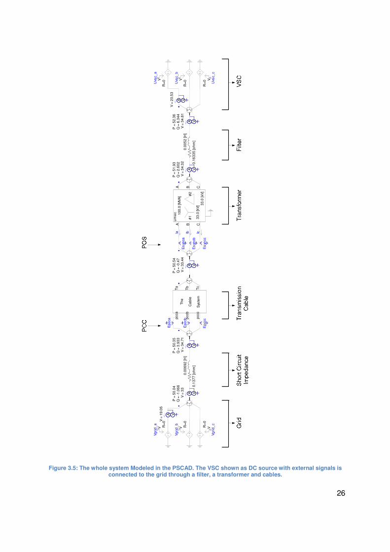
In the light of the above discussions the whole system was modeled in PSCAD and shown in Figure 3.5. The figure clearly shows the various parts of the whole system along with the PCC and the Point of Synchronization (POS). The PLL was synchronized to the voltage at POS which is separated from PCC by the transmission cable. Inside the cable system nine cables were implemented which are shown in the appendix.

3.5. CABLE RESONANCE

At the very beginning of the simulation, transients were observed in the PCC voltage when cables were implemented and are shown in Figure 3.4. It is observed that the frequency of these transients is about 600Hz which is within the band of the positive sequence resonant frequency of the entire system at the PCC.

Figure 3.4: Transients observed in PCC at the beginning of simulation when cables were used

The resonant frequency of the cable system alone was observed to be 13.5 kHz. However, when used within the system the cable impedance along with the grid impedance forms a series resonant circuit at the PCC. This can be characterized by a low impedance path for the harmonic currents at the resonant frequency and results in

SupervisoryControl : Graphs

0.000 0.020 0.040 0.060 0.080 0.100 0.120 ... ... ...

0.00

0.25

0.50

0.75

1.00

1.25

1.50

1.75

2.00

y

absUpcc magUpcc

Vo

lta

ge

[p

.u.]

Time [s]

25

high voltage distortion and over voltages. The short circuit capacity of our grid was considered to be 500 MVA while reactive power requirement of our cable system can be estimated to about 5 MVA. Then the first resonant frequency can be estimated as 10p.u. by the following formula [19]:

-(1. 2) ?#6-/+#! @" This implies that the first resonant frequency at the PCC is approximately 500Hz. This relation also defines that greater the short circuit rating of the grid or the system connected to the cable the higher will be the resonant frequency. It has also been discussed in [19] that the higher the short circuit power level the longer will be the duration of transients.

The high magnitudes of the transients on the contrary are due to the high charging current required by the cable system and the moment when the cable is connected to the system. The over voltages can be decreased if the cable system is energized when the PCC voltage is zero. The peak over voltages during the normal energization of the cable can range up to 2p.u.

3.6. CONTROL ACTION

Now that we have selected the ratings of our system and known the grid integration of our wind farm, it is of great importance to understand how the wind farm should interact with the grid. Grid codes are considered to be a set of technical requirements that any power plant should fulfill in order to maintain power balance along with power quality and to ensure a secure operation of the system. These rules are usually provided by the Transmission System Operators (TSOs) to the Power Plant Operators (PPOs). These rules form the basics of designing the control algorithm for a power plant and generally vary from country to country.

3.6.1. COMMON GRID CODES

In this section we will present an overview of a selected grid codes which are more or less the basic that all the TSO’s require from the power plants. These requirements are usually evaluated according to the characteristics of the grid at the point of common connection (PCC). This is important to understand because these are the requirements set out for the whole farm connection and not at the individual turbine terminals.

As a mandatory requirement the active power output of the wind farm should be provided within specific levels of grid frequency and voltage. Typical requirements, in this regard, required by the E.ON and Swedish grid codes for large wind farms are shown in Figure 3.6 and Figure 3.7 respectively.

26

Figure 3.5: The whole system Modeled in the PSCAD. The VSC shown as DC source with external signals is connected to the grid through a filter, a transformer and cables.

R=

0V R

=0

V R=

0V

0.1

63

35

[oh

m]

0.1

37

7 [o

hm

]

0.0

05

2 [H

]0

.00

69

2 [H

]

R=

0V

R=

0V

R=

0 V

V =

19

.05

VA

P =

50

.04

Q =

-1

.06

6V

= 3

3

VA

P =

50

.54

Q =

-0

.47

V =

33

.44

VA

P =

50

.35

Q =

3.9

33

V =

34

.71

VA

Ep

cca

Ep

ccb

Ep

ccc

Es

ynca

Es

yncb

Es

yncc

Ia Ib Ic

P =

52

.36

Q =

6.3

44

V =

34

.81

VA

V =

20

.53

VA

Vg

rid

_a

Vg

rid

_b

Vg

rid

_c

Uvs

c_a

Uvs

c_b

Uvs

c_c

A B C

A B C

#2

#1 33

.0 [k

V] 3

3.0

[kV

]

10

0.0

[MV

A]

um

ec

P =

51

.93

Q =

2.6

02

V =

34

.32

VA

Th

e

Ca

ble

Sys

tem

pcc

a

pcc

b

pcc

c

Ta

Tb Tc

27

The steady state operational requirements of reactive power in terms of active power are also defined by these regulations. For example E.ON specifies the PQ - operational range for a +/- 5% voltage range of the generation unit as shown in Figure 3.8.

Figure 3.6: Typical active power requirements from offshore wind farms placed by E.ON

Figure 3.7: Typical active power requirements for large wind farms by Svenska Kraftnet

28

Figure 3.8: General PQ characteristics required for grid integration of wind farms

Traditionally, the wind farms were required to disconnect from the grid in case of voltage dips. However, now due to the high penetration of wind power plants into the grid, they are required to have a fault ride through capability. This ride through characteristic is usually given as a function of the magnitude of the voltage dip and time duration and is shown in Figure 3.9 for large wind farms. Now the tripping of the wind farm is only allowed if the voltage level stays sufficiently low for durations which put it into the shaded region.

Figure 3.9: General fault ride through characteristics required by grid codes

3.6.2. ADVANCED GRID OPERATION

Modern wind power plants employ variable speed wind turbines which due to the technological advancements have dedicated control systems. These control systems provide us the opportunity to introduce many advanced control actions enabling Wind power plants to have grid support capability and behave like conventional power plants.

As discussed in the previous section, the modern wind power plants are required to provide fault ride through capability. This implies that a wind power plant should remain in service during normally cleared system faults [20]. Apart from this requirement few

29

TSOs, like EON, even require that a wind farm should support the grid by generating reactive power during a network fault. This is considered to be a grid support functionality known as “Voltage Support” and helps to restore the grid voltage in a more fast and efficient manner.

E.ON requires a wind farm to support grid voltage with increased reactive current injection during Voltage dips or even increased reactive current consumption during voltage swells according to a predefined set points as shown in Figure 3.10. According to this control, if the PCC voltage varies by +/- 5% then, after the detection of the fault, the wind power plant must respond within 20ms by providing or absorbing additional reactive current amounting to at least 2% of the rated current for each percent of voltage dip. A reactive current injection of 1 p.u should be possible in such a scenario.

Figure 3.10: Voltage Support requirements by E.ON grid codes

3.7. CONCLUSION

In this chapter the fully rated converter based wind turbines and their grid integration was discussed in detail. It was realized that for the reactive power control the control of the grid side converter should only be considered, therefore the grid integration of a simple VSC was discussed. In this context the ratings considered for the modeling of our system along with the selection of filter, transformer and grid short circuit capacity was elaborated.

Finally the grid codes for wind farms necessary for the implementation of the control system along with some advanced control actions, which will be viewed as a major focus of our thesis, were highlighted.

30

4. CONTROL DESIGN FOR REACTIVE POWER COMPENSATION

4.1. INTRODUCTION

A simplified model of a VSC connected to an AC system is shown in Figure 4.1. The AC system is an equivalent voltage stiff source representing the voltage at the point of synchronization. The equivalent series inductance and resistance of an L-filter is given as Lf and Rf respectively. The AC system voltage is given by vabc (t) and the VSC voltage is given as uabc

(t).

Figure 4.1: Simplified model of a VSC connected AC system

The Kirchhoff voltage law when applied to the above circuit gives us:

2AB! 3CB! +4 ECB! EF + GB! Different control techniques can be utilized to control the power flow over the grid side VSC. In this chapter we will discuss, the control method along with the design of the controller considered for the implementation of the model in PSCAD.

4.2. CONTROL METHOD

In order to achieve the control of instantaneous active and reactive power that a VSC exchanges with the AC system, usually cascaded control is considered. The control system is implemented in the dq frame of reference due to the fact that the dq frame rotates with the angular grid frequency; hence, all the AC quantities when transformed to it appear as DC quantities. This enables us to implement PI controls in an efficient manner.

Transforming the above equation into αβ frame of reference can be written as:

2ABHI 3CBHI +4 ECBHIEF + GBHI

Then in dq frame of reference the above equation can be written as:

2AB+J 3CB+J +4 ECB+JEF + KL64CB+J + GB+J

31

Where, ωg is the grid angular frequency. The grid angular frequency and the transformation angleM, required for dq transformation, are estimated with the help of phase locked loop (PLL).

On the basis of above system equations, vector control techniques were utilized to implement the cascaded control system. This cascaded control system comprises of an inner vector current controller which controls the instantaneous amplitude of the line current while the outer loop consists of an active power and voltage controller to control the instantaneous power transferred over the PCC or the voltage at PCC respectively. This control scheme is considered to have good dynamic behavior, higher precision and robustness against variations in parameters [21].

It should be mentioned here, for dq transformations a voltage oriented, amplitude invariant system was considered.

4.3. PLL ESTIMATOR

The phase locked loop is used in our system to synchronize with the grid voltage vector GBHIand the transformation angle denoted by M is the grid voltage angle in steady state.

Then the VSC voltage vector in dq frame of reference can be written as [22]:

2AB+J 2ABHINOPQ 2ABHINOPR. Similarly, the grid voltage vector can be written as:

GB+J GBHINOPQ GBHINOPR. Where,

GBHI ,NPQS

Then:

GB+J GBHINOPQ ,NPQSNOPQ ,NP(QSOQ) If M M6, then the grid voltage vector becomes a DC quantity equal to the amplitude of

the grid voltage vector:

GB+J , This describes that the AC system has transformed to a perfect DC system and enforces that the dq frame is only useful if we have the exact knowledge of the angle of the AC system voltage vector. PLL is currently the best known technique to achieve this knowledge of angle.

32

A phase locked loop is defined as a closed loop system in which an estimate M is driven

to its correct value M6by an error signal sinWM6 − MX. When M6 ≈ M then the error signal sinWM6 − MX ≈ 0 and the PLL is said to be phase locked.

We desire that our dq system should be oriented to the grid voltage vector, therefore, the PLL should track the imaginary part of the AC system voltage vector in dq system in order to be perfectly phase locked. As:

GZ,+ , cos(M6 − M) GZ,J , sin(M6 − M)

Then in steady state when M6 ≈ M:

GZ,J ≈ ,(M6 − M) Hence, the error signal is given as:

] GZ,J, WM6 − MX The law governing the PLL can be written as [23]:

L_6 à8 ] M, Lb6 + 2à]

Where, αPLL is regarded as the bandwidth of the PLL while Lb6is the estimated grid

frequency and M, is the estimated grid angle. Then the closed loop transfer function of the PLL can be written as:

cda(e) 2eà + à8e8 + 2eà + à8

The proportional and the integral gains for the PLL can be evaluated from the above equation as:

fg,a 2à f/,a à8

Generally, when used for grid applications the PLL is required to track the positive sequence angle of the grid voltage vector [22]. Therefore, in order to ensure a good rejection of the negative sequence component of the grid voltage low bandwidths for the

33

PLL must be selected [22]. Therefore, a bandwidth of 30 rad/s has been selected. Then the block diagram of PLL is shown in Figure 4.2:

Figure 4.2: Simplified model of a PLL

In order to assess the operation of the PLL a variation of 10 radians was applied in the phase of grid voltages at 6.005 s as shown in Figure 4.3:

Figure 4.3: Phase variation applied in grid voltage

As a result, the PLL which was locked to the previous angle tries to re track the angle in order to phase lock as shown in Figure 4.4. Prior to 6.005 s the time taken by the angle to vary from 0 to 2π radians is around 20 ms as shown in by interval 1 in the Figure 4.4. However, when the voltage variation is observed the time to vary the angle from 0 to 2π radians is reduced to 16.7 ms and 16.4 ms shown by intervals 2 and 3 respectively. Then this time rises again to 18.2 ms, 19.5 ms and finally 20ms which is shown by intervals 4, 5 and 6 respectively. This clearly depicts that the PLL tries to phase lock with

Voltage:abc : Graphs

5.9850 5.9900 5.9950 6.0000 6.0050 6.0100 6.0150 6.0200 6.0250 ... ... ...

-30

-20

-10

0

10

20

30

V [

kV]

Vgrid_a Vgrid_b Vgrid_c

34

the new angle between the intervals 2 to 5, which is a duration of about 70 ms. Therefore, we may conclude that the implemented PLL takes around 70ms to track the new angle post any disturbance applied to the system.

Figure 4.4: Angle tracking by the PLL when grid is subject to phase variation

4.4. CURRENT CONTROLLER

The equation for the voltages in dq reference at the point of synchronization can be written as:

*+ 3h+ + 4 Eh+EF − i4hJ + Z,+

*J 3hJ + 4 EhJEF + i4h+ + Z,J

Then the system can be modeled as in Figure 4.5:

Figure 4.5: Simplified model of the system process

From the above mentioned equations if we neglect the cross coupling and the feed forward terms we get the following equation:

angles:2pi : Graphs

5.950 6.000 6.050 6.100 6.150 6.200 6.005 6.075 0.070

0.0

1.0

2.0

3.0

4.0

5.0

6.0

7.0

y

0.113

0.560

0.447

Min 0.009

Max 6.280

theta_2pi

Time [s]

1 2 3 4 5 6

35

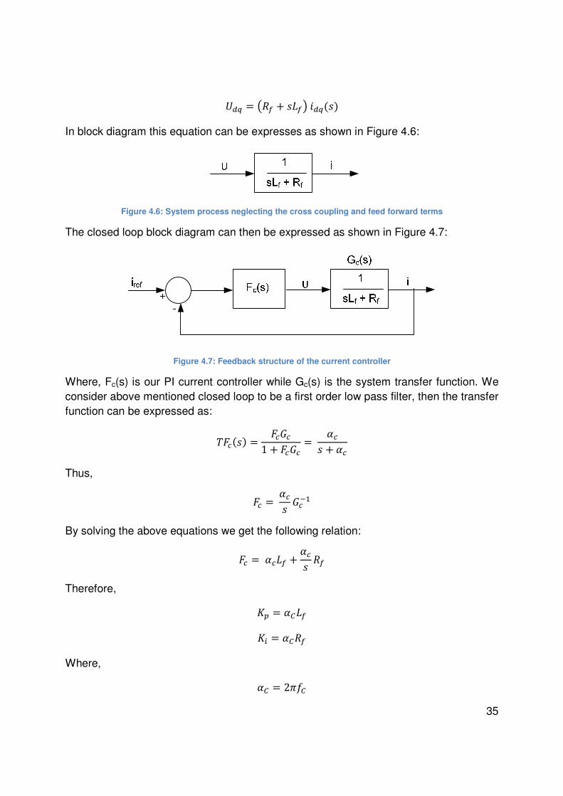
*+J W3 + e4Xj+J(e) In block diagram this equation can be expresses as shown in Figure 4.6:

Figure 4.6: System process neglecting the cross coupling and feed forward terms

The closed loop block diagram can then be expressed as shown in Figure 4.7:

Figure 4.7: Feedback structure of the current controller

Where, Fc(s) is our PI current controller while Gc(s) is the system transfer function. We consider above mentioned closed loop to be a first order low pass filter, then the transfer function can be expressed as:

cd(e) dk1 + dk è + ` Thus,

d è kO By solving the above equations we get the following relation:

d `4 + è 3

Therefore,

fg `l4

f/ `l3

Where,

`l 2ml

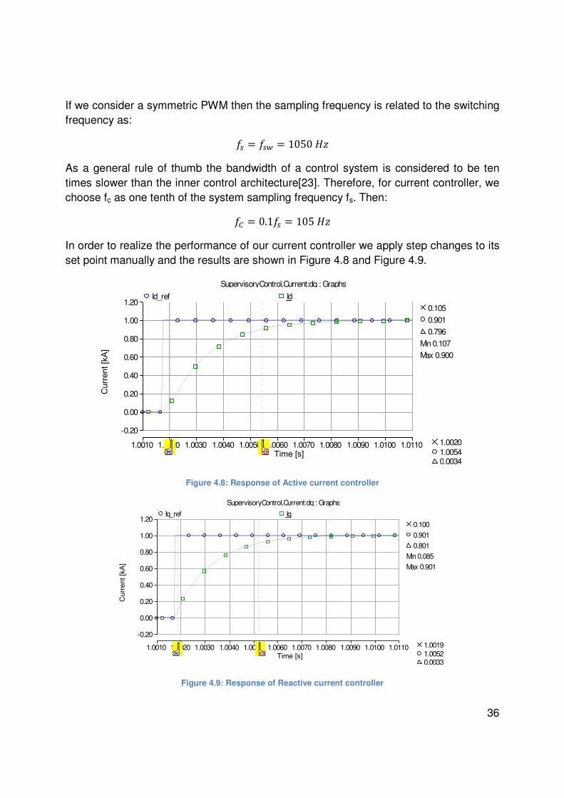
36

If we consider a symmetric PWM then the sampling frequency is related to the switching frequency as:

1050

As a general rule of thumb the bandwidth of a control system is considered to be ten times slower than the inner control architecture[23]. Therefore, for current controller, we choose fc as one tenth of the system sampling frequency fs. Then:

l 0.1 105 In order to realize the performance of our current controller we apply step changes to its set point manually and the results are shown in Figure 4.8 and Figure 4.9.

Figure 4.8: Response of Active current controller

Figure 4.9: Response of Reactive current controller

SupervisoryControl,Current:dq : Graphs

1.0010 1.0020 1.0030 1.0040 1.0050 1.0060 1.0070 1.0080 1.0090 1.0100 1.0110 1.0020 1.0054 0.0034

-0.20

0.00

0.20

0.40

0.60

0.80

1.00

1.20

Id [

A]

0.105

0.901

0.796

Min 0.107

Max 0.900

Id_ref Id

Time [s]

Curr

ent [k

A]


1.0010 1.0020 1.0030 1.0040 1.0050 1.0060 1.0070 1.0080 1.0090 1.0100 1.0110 1.0019 1.0052 0.0033

-0.20

0.00

0.20

0.40

0.60

0.80

1.00

1.20

Iq [

A]

0.100

0.901

0.801

Min 0.085

Max 0.901

Iq_ref Iq

Curr

ent [k

A]

Time [s]

37

The time to rise or rise time is defined as the time taken a signal to rise from a value of 10% to 90% and is used to assess the performance of a control system. Time to rise is evaluated as follows:

F- ln 9`

Where α is the bandwidth of the system under consideration. Therefore, the rise time of our current controller is:

F- ln 9` 3.33e As can be seen from Figure 4.8 and Figure 4.9 the rise time of d axis current and the q axis current have a rise time of about 3.3ms which is in accordance to the designed system.

4.5. ACTIVE POWER CONTROLLER

The active power in dq frame can be calculated as:

32f8 (*+h+ − *JhJ) Where K = 1 for amplitude invariant system. If we consider that our dq-coordinate system is perfectly oriented with the voltage vector then Uq = 0. Therefore the above equation can be rewritten as:

32*+h+ For designing our PI controller we consider the dynamics of the inner controller along with the above mentioned equation. Then the closed loop system can be drawn as shown in Figure 4.10:

38

Figure 4.10: Feedback structure of Active power controller including the inner controller

Where, Fp(s) is the controller while Gp(s) is the system for which the controller is designed. Considering this closed loop system as a first order system, the transfer function of the above system can be written as:

cda(e) dgkg1 + dgkg `ge + `g

Thus,

dg `ge kgO

Then by solving the above closed loop we obtain:

dg 2`g3`*+ + 2`g3*+e Therefore,

fg 2`g3`*+

f/ 2`g3*+

According to the grid codes the active power should increase at least at a gradient of 0.1 p.u. per second. Therefore, the following bandwidths were selected for the system:

`g 2mg

g 0.25

39

Similar to the case of current controller, a step change was applied to the active power controller set point and the results were observed as shown in Figure 4.11. The time to rise was observed to be almost 1.9 s.

Figure 4.11: Simulated step response of active power control system

According to the designed considerations the rise time was found to be:

F- ln 9`g 1.4e The deviation of the obtained rise time from the theoretical one is due to the neglected dynamics of the cable system in the implementation of the control system and the filter applied in the feedback loop of the power controller.

4.6. REACTIVE POWER CONTROL

Typically, reactive power in a power system can be controlled directly by reactive power controller or indirectly by a voltage controller. Both of these controllers have their own control theorems and are discussed below. However, it should be emphasized here that in this thesis voltage controller was only implemented.

4.6.1. REACTIVE POWER CONTROLLER

The reactive power in dq frame can be calculated as:

o −32f8 (*+hJ + *Jh+)

SupervisoryControl,Power : Graphs

0.0 1.0 2.0 3.0 4.0 5.0 6.0 7.0 1.1 3.1 2.0

-10

0

10

20

30

40

50

60

P [

MW

]

5.000

45.000

40.000

Min 5.001

Max 45.000

Pref Ppcc

Time [s]

40

Where K = 1 for amplitude invariant system. If we consider that our dq-coordinate system is perfectly oriented with the voltage vector then Uq = 0. Therefore the above equation can be rewritten as:

o −32 *+hJ Then the reactive power controller gains are evaluated to be the same as that of active power controller.

4.6.2. VOLTAGE CONTROLLER

If we assume that voltage at PCC has slower dynamic behavior then we can apply steady state voltage controller instead of the vector voltage controller. Thus, the phasor of the voltage magnitude at the PCC can be written as:

*all $6h+J

Then it can be evaluated that:

*+,all ≈ −06hJ

Assuming that is always:

*J,all ≈ 0

Then, we conclude that:

|*|all −06hJ

Then the closed loop system can be drawn as in Figure 4.12:

Figure 4.12: Feedback architecture of voltage control system

It is worth noting here that the dynamics of the inner controller are considered to be 1 as the inner controller is assumed to be much faster than the outer controller. Then:

cd(e) dk1 + dk `e + `

41

Thus,

d `e kO Solving the above closed loop we obtain:

d − `e06

Therefore:

f/ −`06

The TSOs require that the voltage at the point of common connection should be maintained within +/- 5% of the nominal voltage value. Therefore, we introduced a droop characteristic in the voltage controller which enables us to achieve a higher regulation range of voltage. The droop appears as gain Ksl in the control diagram and is shown in Figure 4.13. The value of droop in per units is considered to be 0.05.

Figure 4.13: Feedback voltage control system with droop characteristics

It should be emphasized here that usually in a weak grid connected system; voltage controller is preferred due to the voltage variation issue. In this case if the system requires reactive power then the output of the reactive power should be added into the voltage controller error signal to meet the grid extra reactive power requirement [24].

A step change was applied to the voltage controller as well in order to assess its response. In Figure 4.14 it can be seen the voltage controller is able to push the PCC voltage a bit higher but is never able to reach the exact value. The reason for this is the introduction of the droop characteristics within the control system which limit the integrator from nullifying the error completely.

42

Figure 4.14: Simulated step response of voltage control system

4.7. SATURATION AND INTEGRATION ANTI-WINDUP

In any system implementation, there always are some limits in which the system should be operated. These limits usually originate from the actuators applied in the control system. If the control system tries to exceed these limits then the system leads to nonlinear behavior. In this section such scenarios will be evaluated in detail by considering the inner and outer control loops.

4.7.1. INNER CONTROLLER

It can be shown that the switching signals to the three legged VSC switches can be combined in eight ways [22]. The resulting voltage vectors draw a hexagon in the αβ coordinate system. The VSC is capable of delivering the voltages within this hexagon [22]. If amplitude invariant system is considered then the maximum achievable voltage

with linear modulation isqrs√u shown by inscribed circle inside the hexagon in Figure

4.15[8].

If the reference voltage vector exceeds the boundary of the hexagon, then the VSC is unable to deliver the demanded voltage and is said to have been saturated. If the reduction of voltage is not considered during this event then the system performance is reduced [22].

Several techniques regarding the limitation of the reference voltage vector have been developed to avoid this issue effectively [25]. In this thesis Minimum Amplitude Error (MAE) method was utilized. In MAE the voltage amplitude error is minimized by selecting the voltage vector, in xy coordinate system, on the hexagon boundary nearest

VoltageRegulator : Graphs

1.000 1.025 1.050 1.075 1.100 1.125 1.150 1.175 1.200 1.018 1.164 0.145

0.9950

1.0000

1.0050

1.0100

1.0150

1.0200

1.0250

1.0300

1.0350

y

1.000

1.024

0.024

Min 1.000

Max 1.024

Upccref absUpcc

Time [s]

43

the reference voltage vector[22][25]. Hence, the components of the reduced reference voltage vector along with αβ to xy coordinate system transformation angle can be written as follows [25]

2v,@/7 *+√3

2Z,@/7 w 2Z,-" , x2Z,-"x ≤ *+3ezW2Z,-"X*+3 , x2Z,-"x > *+3

MvZ 1 + 2(e − 1)~ m6

Where, s is the sector in hexagon where the reference voltage vector is located.

If the saturation occurs then due to the MAE algorithm, the output voltage vector will be smaller than the system demanded voltage vector. In this case, the integrator of the current controller will integrate the current error and as a consequence the integration term can become very large because the output voltage cannot be increased, thus reducing the current error. This phenomenon is called integrator windup [22].

Figure 4.15: Hexagon limitation region for voltage vector of three phase VSC for amplitude invariant system

In order to avoid the integrator windup back calculation method was implemented. According to this method integrator input error signal is modified in case of saturation in order to account the limited VSC control voltage. Therefore, the modified input error signal to the integrator was found to be:

N N + 1fg W*,@/7+J − *+J X

44

Then, the complete closed loop system with cross coupling terms, anti-windup and saturation block is shown in Figure 4.16.

Figure 4.16: Current control loop with saturation and anti-windup

4.7.2. OUTER CONTROLLER

In power systems, all the equipment is designed for a particular voltage and current rating. These ratings should be followed in order to avoid the system failures. The inner controller sets the reference voltage vector for the VSCs and the saturation scenario for it was discussed earlier. However, the outer controller sets the reference current vector which the system should follow. If the outer control loop does not limit the reference current vector and the inner controller hits saturation then the integrator part in the outer controllers wind up to large values and should also be avoided.

Therefore, the current reference vector was limited to the maximum rating of the system current amplitude and by back calculation the modified integrator error signal for active and reactive power controllers was evaluated as:

Na, N + 1fga Wh-",@/7+ − h-"+ X N, N + 1fg Wh-",@/7J − h-"J X

It should be mentioned here that this modified error signal is not required for the voltage controller due to the droop characteristics which limits its output to a certain value.

Then, the complete closed loop system for active power controller with an anti-windup is shown in Figure 4.17. Note the whole system is drawn in per units. Also, the reactive power controller will observe the same system except for it will be tracking the reactive current component iq and therefore is not shown here.

45

Figure 4.17: Power control loop with anti-windup

4.8. VOLTAGE SUPPORT ALGORITHM

As discussed earlier, in the section of grid codes, during faults the grid is often required to support the grid with reactive current injection within 20ms by following a fixed characteristic curve.

In this context, the voltage at the point of common connection was continuously compared to a lower threshold value of 0.95p.u and an upper threshold value of 1.05p.u. If the voltage was recognized to be below or above the threshold values then the reference reactive current level (in per units) to be injected in the system was evaluated as follows:

hJ,-"J 2W*gg-"!@. − *g--".X − hJg-"!@. In actual systems, the current usually has harmonics due to the VSC switching. Therefore, in order to obtain the prefault value of the reactive current the reference reactive current signal was investigated instead of the actual system current. Also, it should be mentioned here that the voltage support control was sustained even after the voltage recovery for a further 500ms in accordance to the grid code. This is generally required for an efficient and fast recovery of the grid voltage.

During the actuation of voltage support algorithm few things should be considered:

• The active power output should be limited in order to meet the required reactive current value.

• The saturation of the inner controller should continuously be investigated. If the inner controller is observed to have saturated then the outer controller should be frozen in order to avoid further saturation of the VSC voltage vector.

46

4.9.ACTIVE POWER REFERENCE

The reference active power was calculated by the active and reactive power delivery strategy described by [26] suggested in accordance with the E.ON grid codes:

∗ ?32*h8 − o∗8 o∗ 3*h 1 − **

Where, IN and UN are the nominal current and voltage peak values of the system, respectively, while U+ is the positive sequence voltage measured at the PCC. In our system positive sequence voltage was realized by filtering the PCC voltage through a low pass filter with a time constant of 0.01s while the nominal current and voltage values are the base current and voltage ratings of our system.

From the above equations it was analyzed that when the reactive power reference is zero then the active power reference is the rated converter power i.e. 100MW. In real systems the active power production is dependent upon the amount of wind power available which may not always be available. Therefore, this active power reference was restricted to a maximum of 50MW for the simulations executed by multiplying the reference power value obtained by the above mentioned equations by a factor of 0.5.

4.10. TIME DELAY

A pure time delay is generally represented by the transfer function:

c. d NO

Where, T is the delay time.

The point of common coupling is usually located at far distances from the wind farm and the supervisory control system. Thus, the measured PCC voltage used in the outer loop is delayed by almost 2 to 10 cycles of the system frequency. The grid operators require a high bandwidth for the voltage controller to help restore the grid voltage which under the influence of these delays can impact the performance of the system and even lead to voltage or power instability. It should be noted here that in this thesis the time delays of 50ms, 100ms, 150ms and 200ms were studied to express the findings.

4.11. CONCLUSION

In this chapter different parts of a controller which were necessary to be realized in order to attain the best functioning of our system were discussed. The whole system was implemented in the dq frame of reference. To realize the angle for transformation a PLL was designed. To have a control over the line current a vector current controller was

47

implemented. The set point for the d axis current was evaluated from the active power controller, while the q axis current set point was evaluated by the voltage controller. The range of controllability of the voltage controller was enhanced by adding droop characteristics to the voltage controller.

48

5. RESULTS AND SIMULATION

5.1. INTRODUCTION

In this chapter, we will observe the dynamic behavior of our system with the help of different plots obtained from simulations. We will simulate a voltage dip at the grid by decreasing the amplitude of the grid voltage and analyze the dynamics of the system at the PCC. Therefore, a phase jump will also be observed at the PCC along with the voltage dip. The magnitude of the remaining grid voltage was considered to be 0.7p.u. during the voltage dip. The dip was applied at 8.5 s and was removed at 9.5 s as shown in Figure 5.1. It must be noted that the two events were considered to be instantaneous or in other words no ramp down or ramp up functions were applied to the voltage profile. The results were obtained considering either the conventional voltage regulator or the voltage support algorithm suggested by the E.ON grid codes and was discussed in the earlier chapters. The results obtained from the two types of regulation schemes were then compared to fully understand the dynamic behavior of the system. It should also be remarked that the output of the conventional voltage regulator was limited to a certain level in order to avoid the current controller to saturate during the voltage dip.

Additionally, in order to identify the transients associated to the capacitance of the cable occurring at the PCC a series R and L of the equivalent cable system were used instead of the transmission cable. The series R and L of the equivalent cable system, from here onwards, will be referred as Zcable.

Figure 5.1: Balanced three phase dip of 0.7 p.u. applied to the grid at 8.5s. The dip was removed at 9.5s. It is observed that the voltage dip is instantaneous and that the voltage magnitude falls from 26.94kV to 18.858kV

during the voltage dip.

Voltage:abc : Graphs

8.40 8.60 8.80 9.00 9.20 9.40 9.60 ... ... ...

-30

-20

-10

0

10

20

30

V [

kV]

Vgrid_a Vgrid_b Vgrid_c

Time[s]

49

5.2. RESULTS WITH CONVENTIONAL VOLTAGE CONTROLLER

In this section we will review the behavior of a conventional voltage regulator when the system has 0ms, 50ms and 100ms time delays. Initially we will review the results by using Zcable only and then they will be reviewed by using the complete transmission cable system.

5.2.1. USING Zcable AND NO TIME DELAY

The voltage profile observed during the dip event is shown in Figure 5.2.

Figure 5.2: PCC voltage magnitude profile in dq-coordinate system (absUpcc is the instantaneous curve while magUpcc is the filtered signal observed by the voltage controller) when a dip is applied over the grid voltage.

The plots were taken when no time delay exists.

As can be observed the voltage maintains a value of 1 p.u. prior to the dip event. Then the dip is applied and the voltage falls to 0.7p.u. At 9.5 s the voltage recovers and the voltage is again maintained to a value of 1 p.u. If we look closely to the dq components of the PCC voltage, shown in Figure 5.3, we observe that the transients occur in the q component when the dip is applied or removed.

These transients in the q component of the PCC voltage are, firstly, due to the phase angle jump which occurs at the PCC as a consequence to the change in the grid voltage. Secondly, they are due to the time taken by the PLL to phase lock, which is almost 70ms in our case, following a disturbance occurring in the system. The influence of these phenomena is also prominent in the curves of active power shown in Figure 5.4. It can also be observed in Figure 5.3 that the q component of the PCC voltage is not exactly zero throughout the simulation. This is because the whole system is not


8.40 8.60 8.80 9.00 9.20 9.40 9.60 ... ... ...

0.700

0.750

0.800

0.850

0.900

0.950

1.000

1.050

1.100

V [

p.u]

absUpcc magUpcc

Time [s]

50

synchronized to the voltage at PCC but is synchronized to the voltage at the transformer Y side.

Figure 5.3: d and q components of the PCC voltage over the dip event. The plots were taken when no time delay exists within the system.

Figure 5.4: Active power profile during the event of voltage dip. The plots were taken when no time delay exists within the system. Pref is the reference applied while Ppcc is the power transferred over the PCC.

It can additionally be observed from the active power curves that the active power reference also decreases, in accordance to the PCC voltage, in order to enhance the

Voltage:dq : Graphs

8.40 8.60 8.80 9.00 9.20 9.40 9.60 ... ... ...

-5.0

0.0

5.0

10.0

15.0

20.0

25.0

30.0

35.0

V [

kV]

Upcc_d Upcc_q

Time [s]


8.40 8.60 8.80 9.00 9.20 9.40 9.60 ... ... ...

30.0

35.0

40.0

45.0

50.0

55.0

P [

MW

]

Pref Ppcc

Time [s]

51

reactive power injection capability of the system. It can be observed that the Pref decreases by almost 27%.

The reactive power curve, shown in Figure 5.5, in addition to the PCC voltage, shown in Figure 5.2, depict that the voltage regulator injects reactive current during the dip which as a result pushes the voltage magnitude to a value of about 0.8p.u. As the purpose of this thesis is not to investigate the mitigation of the dip, therefore, as discussed earlier the amount of reactive current is limited in accordance to the voltage support requirements, presented in the E.ON grid codes, in order to avoid the saturation of our control system during the dip.

Figure 5.5: Reactive power profile over the entire dip event. The plot was taken when no time delay exists within the system. The reactive current is limited according to the voltage support requirements placed by

E.ON., therefore, the reactive power is limited to almost 40MVArs.

If we now observe the voltage recovery transients in the reactive power, Figure 5.7 and the PCC voltage, Figure 5.6, we conclude that the filtered PCC voltage observed by the voltage regulator rises from the lower threshold value of 0.95p.u at about 9.5037s. At this instant the control system realizes the system voltage recovery. At 9.5 s when the system voltage actually recovers the inner controller is pushed into the saturation region. In order to avoid unnecessary saturation of the system the control system freezes the outer control loop until the dip recovery is detected. Thus, at 9.5037s when the dip recovery is detected the outer control returns to action and the voltage controller as a consequence decreases the reactive current reference to a range where the active current delivery capability of the system is restored. However, the saturation of the inner controller still persists, therefore, the inner controller further takes around 2ms to return from the saturation state. Once, the inner controller has recovered from the saturation

Power : Graphs

8.40 8.60 8.80 9.00 9.20 9.40 9.60 ... ... ...

-10

0

10

20

30

40

50

60

Q [

MV

Ar]

Qpcc

Time [s]

52

region the current controller influences the system current to follow the reference currents again according to the designed characteristics.

Figure 5.6: PCC voltage profile when the grid voltage recovers. The plots were taken when no time delay exists within the system (absUpcc is the instantaneous curve while magUpcc is the filtered signal observed

by the voltage controller). The voltage crosses the threshold of 0.95p.u. at 9.5037s.

Figure 5.7: Reactive power profile when the grid voltage recovers. The plots were taken when no time delay exists within the system.


9.4950 9.5000 9.5050 9.5100 9.5150 9.5200 9.5250 9.5300 ... ... ...

0.750

0.800

0.850

0.900

0.950

1.000

1.050

1.100

V [

p.u]

absUpcc magUpcc

Time [s]

Power : Graphs

9.4950 9.5000 9.5050 9.5100 9.5150 9.5200 9.5250 9.5300 ... ... ...

-10

0

10

20

30

40

50

60

Q [

MV

Ar]

Qpcc

Time [s]

53

Figure 5.8: Active power profile when the grid voltage recovers. Pref is the reference active power while Ppcc is the instantaneous power transferred over the PCC. The plots were taken when no time delay exists within

the system.

Figure 5.9: Active current profile when the grid voltage recovers. Id_ref is the reference set by the power controller while Id is the instantaneous active current. The plots were taken when no time delay exists within

the system.


9.4950 9.5000 9.5050 9.5100 9.5150 9.5200 9.5250 9.5300 ... ... ...

30.0

35.0

40.0

45.0

50.0

55.0

P [

MW

]

Pref Ppcc

Time [s]


9.460 9.480 9.500 9.520 9.540 9.560 9.580 9.600 9.620 ... ... ...

0.70

0.80

0.90

1.00

1.10

1.20

Id [

A]

Id_ref Id

Time [s]

54

Figure 5.10: Reactive current profile when the grid voltage recovers. Iq_ref is the reference reactive current set by the voltage controller while Iq is the instantaneous reactive current flowing in the system. The plots

were taken when no time delay exists within the system.

Figure 5.11: Error to the anti-windup of the current controller showing saturation. Dud is the error in the d component while Duq is the error in the q component. The plots are shown for saturation when the grid

voltage recovers. The plots were taken when no time delay exists within the system.

The current plots over the entire dip event are shown in Figure 5.12 and Figure 5.13. These curves clearly explain that the control system is able to control the current values within the nominal range throughout the simulation.


9.4950 9.5000 9.5050 9.5100 9.5150 9.5200 9.5250 9.5300 ... ... ...

-1.40

-1.20

-1.00

-0.80

-0.60

-0.40

-0.20

0.00

0.20

Iq [

A]

Iq_ref Iq

Time [s]

CurrentController : Graphs

9.4950 9.5000 9.5050 9.5100 9.5150 9.5200 9.5250 9.5300 ... ... ...

-5.0

-4.0

-3.0

-2.0

-1.0

0.0

1.0

V [

kV]

Dud Duq

Time [s]

55

Figure 5.12: Active current profile over the entire dip event. Id_ref is the reference active current while Id is the instantaneous current flowing in the system. The plots were taken when no time delay exists within the

system.

Figure 5.13: Reactive current profile over the entire dip event. Iq_ref is the reference active current while Iq is the instantaneous current flowing in the system. The plots were taken when no time delay exists within the

system.

5.2.2. WITH TRANSMISSION CABLES AND NO TIME DELAY

The voltage magnitude profile observed at the PCC over the entire dip event is shown in Figure 5.14. The curve depicts that there are two different sets of transients occurring over the entire simulation and that the magnitude of the transients have increased.


8.40 8.60 8.80 9.00 9.20 9.40 9.60 ... ... ...

0.70

0.80

0.90

1.00

1.10

1.20

Id [

A]

Id_ref Id

Time [s]


8.40 8.60 8.80 9.00 9.20 9.40 9.60 ... ... ...

-1.40

-1.20

-1.00

-0.80

-0.60

-0.40

-0.20

0.00

0.20

Iq [

A]

Iq_ref Iq

Time [s]

56

Figure 5.14: PCC voltage profile over the entire dip event when transmission cable is used and no time delay exists within the system. absUpcc is the instantaneous voltage magnitude while magUpcc is the filtered input

to the voltage controller.

The first set of transients is the one when the dip is applied and is shown in Figure 5.15.

Figure 5.15: Transients in the PCC voltage due to the cable de-energization when the dip occurs. The plots were taken when the transmission cable is used and no time delay exists within the system. absUpcc is the

instantaneous voltage magnitude while magUpcc is the filtered voltage signal to the voltage controller.


8.40 8.60 8.80 9.00 9.20 9.40 9.60 9.80 ... ... ...

0.40

0.50

0.60

0.70

0.80

0.90

1.00

1.10

1.20

1.30

y

absUpcc magUpcc

Time [s]


8.480 8.500 8.520 8.540 8.560 8.580 8.600 8.620 ... ... ...

0.40

0.50

0.60

0.70

0.80

0.90

1.00

1.10

y

absUpcc magUpcc

Time [s]

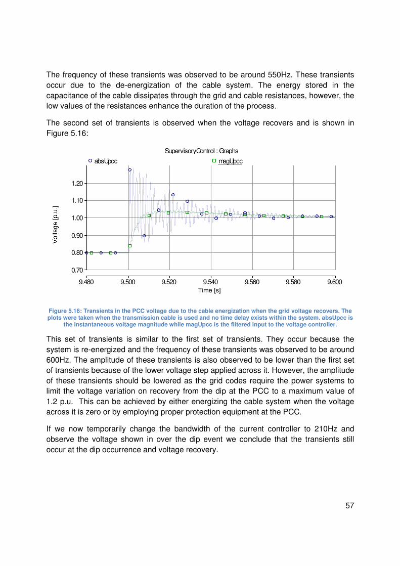
57

The frequency of these transients was observed to be around 550Hz. These transients occur due to the de-energization of the cable system. The energy stored in the capacitance of the cable dissipates through the grid and cable resistances, however, the low values of the resistances enhance the duration of the process.

The second set of transients is observed when the voltage recovers and is shown in Figure 5.16:

Figure 5.16: Transients in the PCC voltage due to the cable energization when the grid voltage recovers. The plots were taken when the transmission cable is used and no time delay exists within the system. absUpcc is

the instantaneous voltage magnitude while magUpcc is the filtered input to the voltage controller.

This set of transients is similar to the first set of transients. They occur because the system is re-energized and the frequency of these transients was observed to be around 600Hz. The amplitude of these transients is also observed to be lower than the first set of transients because of the lower voltage step applied across it. However, the amplitude of these transients should be lowered as the grid codes require the power systems to limit the voltage variation on recovery from the dip at the PCC to a maximum value of 1.2 p.u. This can be achieved by either energizing the cable system when the voltage across it is zero or by employing proper protection equipment at the PCC.

If we now temporarily change the bandwidth of the current controller to 210Hz and observe the voltage shown in over the dip event we conclude that the transients still occur at the dip occurrence and voltage recovery.


9.480 9.500 9.520 9.540 9.560 9.580 9.600 ... ... ...

0.70

0.80

0.90

1.00

1.10

1.20

y

absUpcc magUpcc

Time [s]

58

Figure 5.17: PCC voltage profile over the entire dip event when bandwidth of the current controller changed to 210Hz, transmission cable is used and no time delay exists within the system. absUpcc is the instantaneous voltage magnitude while magUpcc is the filtered input to the voltage controller.

The transients, shown in Figure 5.18 and Figure 5.19 , were still found to have almost the same frequency as were observed in Figure 5.15 and Figure 5.16. Similar results were found when the voltage controller was made a bit faster while keeping the current controller bandwidth at 210 Hz shown in Figure 5.20 and Figure 5.21.

Figure 5.18: Transients in the PCC voltage due to the cable de-energization when the dip occurs. Current controller bandwidth changed to 210 Hz. The plots were taken when the transmission cable is used and no time delay exists within the system. absUpcc is the instantaneous voltage magnitude while magUpcc is the

filtered input to the voltage controller.


8.40 8.60 8.80 9.00 9.20 9.40 9.60 9.80 ... ... ...

0.40

0.50

0.60

0.70

0.80

0.90

1.00

1.10

1.20

1.30

y

absUpcc magUpcc

Time [s]


8.480 8.500 8.520 8.540 8.560 8.580 8.600 ... ... ...

0.40

0.50

0.60

0.70

0.80

0.90

1.00

1.10

y

absUpcc magUpcc

Time [s]

59

Figure 5.19: Transients in the PCC voltage due to the cable energization when the grid voltage recovers. Current controller bandwidth changed to 210 Hz. The plots were taken when the transmission cable is used

and no time delay exists within the system. absUpcc is the instantaneous voltage magnitude while magUpcc is the filtered input to the voltage controller.

Figure 5.20: Transients in the PCC voltage due to the cable de-energization when the dip occurs. Current controller bandwidth changed to 210 Hz and voltage controller made twice as faster. The plots were taken

when the transmission cable is used and no time delay exists within the system. absUpcc is the absUpcc is the instantaneous voltage magnitude while magUpcc is the filtered input to the voltage controller.


9.490 9.500 9.510 9.520 9.530 9.540 9.550 9.560 9.570 9.580 9.590 9.600 ... ... ...

0.70

0.80

0.90

1.00

1.10

1.20

y

absUpcc magUpcc

Time [s]


8.490 8.500 8.510 8.520 8.530 8.540 8.550 8.560 8.502 8.527 0.025

0.40

0.50

0.60

0.70

0.80

0.90

1.00

1.10

y

0.903

0.774

-0.128

Min 0.738

Max 0.903

absUpcc magUpcc

60

Figure 5.21: Transients in the PCC voltage due to the cable energization when the grid voltage recovers. Current controller bandwidth changed to 210 Hz and voltage controller made twice as faster. The plots were

taken when the transmission cable is used and no time delay exists within the system. absUpcc is the instantaneous voltage magnitude while magUpcc is the filtered input to the voltage controller.

This clearly depicts that these transients are independent of the implemented control system. As the transients are observed in the PCC voltage, thus, we may conclude that due to the consideration of steady state PCC voltage conditions while implementing the voltage controller our control system is unable to control these transients.

Apart from the above mentioned transients the behaviour of the system is almost similar to the one obtained for the case with Zcable. The reactive power genereted by the cable influences the value of the reactive current component which flows through the system during the nominal operation. The curves obtained for active and reactive power and currents during the simulation are Figure 5.22 and Figure 5.23 respectively.

It should also be noted that due to the high charging current required by the cable system during energization or voltage recovery the peak current and power values are of higher values. Also, the recovery time from the saturation event of the inner controller is almost the same.


9.4900 9.4950 9.5000 9.5050 9.5100 9.5150 9.5200 9.5250 9.5300 9.5350 9.5400 9.5008 9.5195 0.0187

0.70

0.80

0.90

1.00

1.10

1.20

1.30

y

0.817

1.046

0.229

Min 0.817

Max 1.048

absUpcc magUpcc

Time [s]

Voltage [p.u

.]

61

Figure 5.22: Active power profile over the entire dip event. Pref is the reference power while Ppcc is the power transferred over the PCC. The plots were obtained with no delays and by using a cable system.

Figure 5.23: Reactive power profile over the entire dip event. Qpcc is the reactive power transferred over the PCC. The plots were obtained with no delays and by using a cable system.


8.00 8.50 9.00 9.50 10.00 10.50 11.00 11.50 ... ... ...

10

20

30

40

50

60

70

y

Pref Ppcc

Time [s]

Power : Graphs

8.20 8.40 8.60 8.80 9.00 9.20 9.40 9.60 9.80 ... ... ...

-20

-10

0

10

20

30

40

50

60

y

Qpcc

Time [s]

62

Figure 5.24: Reactive power profile when the grid voltage recovers. Transients due to the saturation of the inner controller start at 9.5 s. Then the reactive power suddenly reduces to a lower value signifying the

detection of voltage recovery.

Figure 5.25: Reactive current profile over the entire dip event. No delays were implemented and cable was modeled. Iqref is the reference reactive current set by the voltage controller while Iq is the current flowing

within the system.

Power : Graphs

9.480 9.500 9.520 9.540 9.560 9.580 9.600 9.620 9.640 9.660 ... ... ...

-10

0

10

20

30

40

50

60

y

Qpcc

Time [s]


8.40 8.60 8.80 9.00 9.20 9.40 9.60 9.80 ... ... ...

-1.40

-1.20

-1.00

-0.80

-0.60

-0.40

-0.20

0.00

0.20

y

Iq_ref Iq

Time [s]

63

Figure 5.26: Active current profile over the entire dip event. Active current Id deviates from the reference Id_ref at the voltage recovery with huge rate of change. The system has no time delays and cable system was

used.

Figure 5.27: Reactive current profile when the grid voltage recovers. It is observed that the reference does not change for some time after the voltage recovery at 9.5s due to the filtered input of voltage controller which

leads to saturation of current controller. Later on the controller is reset to bring the current controller within the controllable range. Cable system was used and no delays were implemented.


8.40 8.60 8.80 9.00 9.20 9.40 9.60 9.80 10.00 ... ... ...

0.50

0.60

0.70

0.80

0.90

1.00

1.10

1.20

1.30

y

Id_ref Id absUpcc

Time [s]


9.490 9.500 9.510 9.520 9.530 9.540 9.550 9.560 ... ... ...

-1.40

-1.20

-1.00

-0.80

-0.60

-0.40

-0.20

0.00

0.20

y

Iq_ref Iq

Time [s]

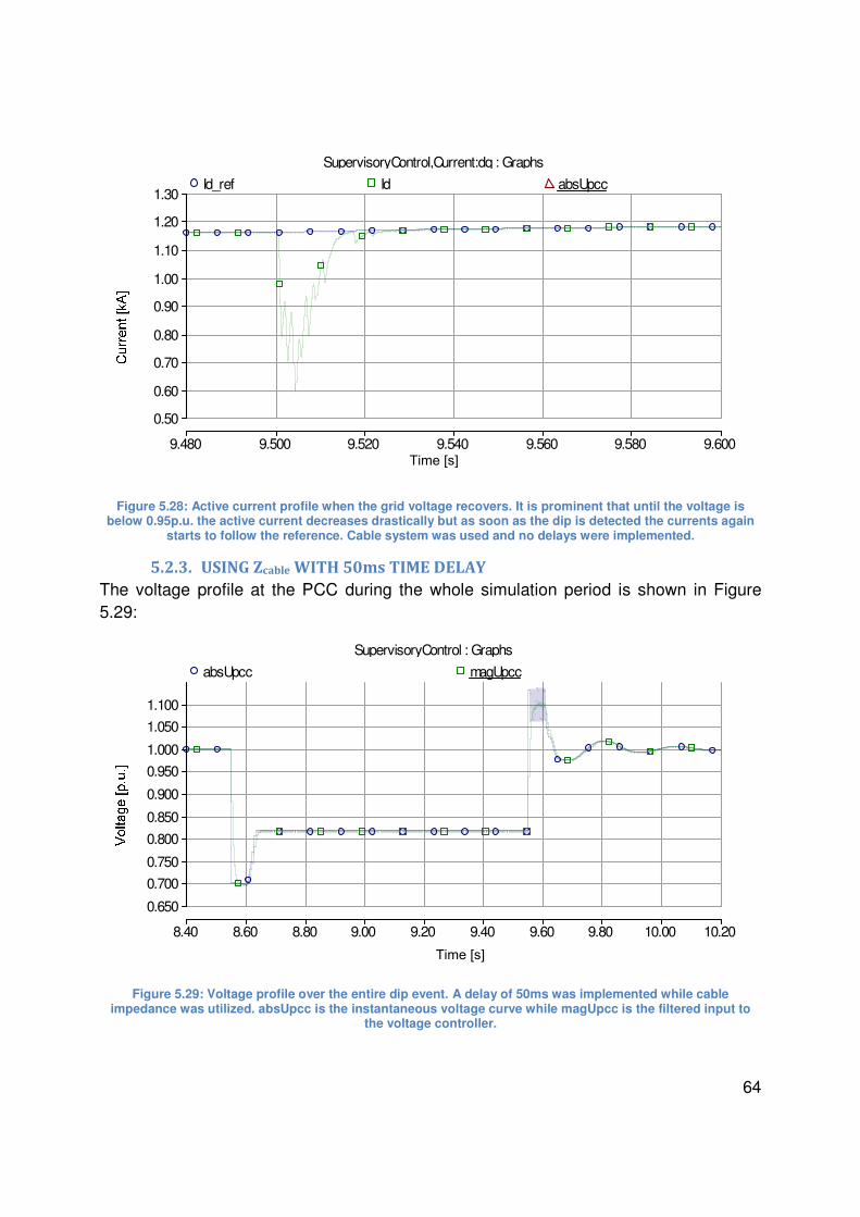
64

Figure 5.28: Active current profile when the grid voltage recovers. It is prominent that until the voltage is below 0.95p.u. the active current decreases drastically but as soon as the dip is detected the currents again

starts to follow the reference. Cable system was used and no delays were implemented.

5.2.3. USING Zcable WITH 50ms TIME DELAY

The voltage profile at the PCC during the whole simulation period is shown in Figure 5.29:

Figure 5.29: Voltage profile over the entire dip event. A delay of 50ms was implemented while cable impedance was utilized. absUpcc is the instantaneous voltage curve while magUpcc is the filtered input to

the voltage controller.


9.480 9.500 9.520 9.540 9.560 9.580 9.600 ... ... ...

0.50

0.60

0.70

0.80

0.90

1.00

1.10

1.20

1.30

y

Id_ref Id absUpcc

Time [s]


8.40 8.60 8.80 9.00 9.20 9.40 9.60 9.80 10.00 10.20 ... ... ...

0.650

0.700

0.750

0.800

0.850

0.900

0.950

1.000

1.050

1.100

y

absUpcc magUpcc

Time [s]

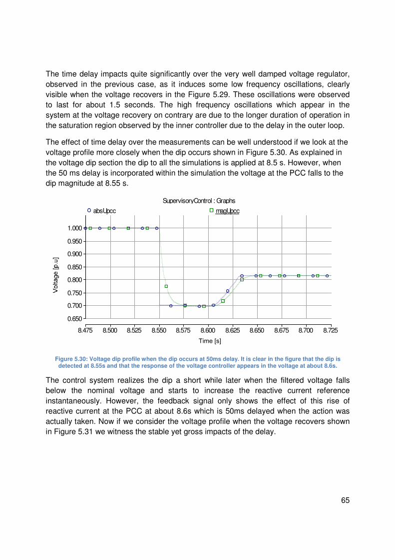
65

The time delay impacts quite significantly over the very well damped voltage regulator, observed in the previous case, as it induces some low frequency oscillations, clearly visible when the voltage recovers in the Figure 5.29. These oscillations were observed to last for about 1.5 seconds. The high frequency oscillations which appear in the system at the voltage recovery on contrary are due to the longer duration of operation in the saturation region observed by the inner controller due to the delay in the outer loop.

The effect of time delay over the measurements can be well understood if we look at the voltage profile more closely when the dip occurs shown in Figure 5.30. As explained in the voltage dip section the dip to all the simulations is applied at 8.5 s. However, when the 50 ms delay is incorporated within the simulation the voltage at the PCC falls to the dip magnitude at 8.55 s.

Figure 5.30: Voltage dip profile when the dip occurs at 50ms delay. It is clear in the figure that the dip is detected at 8.55s and that the response of the voltage controller appears in the voltage at about 8.6s.

The control system realizes the dip a short while later when the filtered voltage falls below the nominal voltage and starts to increase the reactive current reference instantaneously. However, the feedback signal only shows the effect of this rise of reactive current at the PCC at about 8.6s which is 50ms delayed when the action was actually taken. Now if we consider the voltage profile when the voltage recovers shown in Figure 5.31 we witness the stable yet gross impacts of the delay.


8.475 8.500 8.525 8.550 8.575 8.600 8.625 8.650 8.675 8.700 8.725 ... ... ...

0.650

0.700

0.750

0.800

0.850

0.900

0.950

1.000

y

absUpcc magUpcc

Time [s]

66

Figure 5.31: Oscillations observed in the system when the grid voltage recovers and the system has 50ms delay. High frequency transients occur when the dip occurs and the detection of the dip by the control

algorithm. After the dip is detected low frequency transients appear in the voltage.

In the first section we observe the high frequency transients, of almost 300Hz, proclaiming the operation of our inner controller in the saturation region of almost 0.07 p.u. or 1900V peak to peak.

Prior to the fault clearance the wind farm delivered a certain amount of reactive current to the grid. Thus, when the system recovers, due to the non-detection of the system recovery, the voltage controller still maintains the same amount of reactive current. The current controller, due to its instantaneous nature, as a result tries to push the VSC voltage to a higher value and soon hits the limit.

Figure 5.32: High frequency transients of about 300 Hz observed at voltage recovery prior to voltage recovery detection due to the saturation of the inner controller.


9.40 9.50 9.60 9.70 9.80 9.90 10.00 10.10 10.20 ... ... ...

0.750

0.800

0.850

0.900

0.950

1.000

1.050

1.100

y

absUpcc magUpcc

Time [s]


9.540 9.550 9.560 9.570 9.580 9.590 9.600 9.610 9.620 ... ... ...

1.040

1.060

1.080

1.100

1.120

1.140

y

absUpcc magUpcc

Time [s]

67

This means that during the flow of these transients we lost our controllability over the currents flowing within our system. The effect is more prominent in the Id or the active current shown in Figure 5.33. Although the magnitude of the current flowing within the system is still within the nominal range but the direction of the flow of active current changed to the opposite direction i.e. from converter to grid it changed to grid to converter. This shows that the fully rated converters installed should have the damping resistors installed at the DC link in order to burn out the excess amount of active power travelling towards it. The second important factor which should be considered here is the time taken for this transition to occur which is even less than one grid cycle. The switches or the other equipment installed should be carefully selected to survive this transition of currents.

Figure 5.33: Active current profile at grid voltage recovery. The current falls until the dip is detecting clearly showing the uncontrolled operation of the current controller. Once the dip is detected the control system is

able to push the current is pushed to follow the reference.

After the system realizes the recovery of voltage the time to recover to the nominal operation or the controlled operation is almost the same as was discussed in the previous section. However, in this case we observe that the system voltage takes some overshoots shown in Figure 5.34 before settling to the exact voltage level.


9.400 9.450 9.500 9.550 9.600 9.650 9.700 ... ... ...

-0.75

-0.50

-0.25

0.00

0.25

0.50

0.75

1.00

1.25

1.50

y

Id_ref Id

Time [s]

68

Figure 5.34: Low frequency oscillations observed in PCC voltage with 50ms delay at the recovery of grid voltage. It clearly shows that the system is still damped and within a controllable region.

In order to understand these oscillations let us consider the instantaneous reactive current profile shown in Figure 5.35. As observed and discussed when the voltage recovers the system does not realize it until 9.55s. However, due to the operation of the system in the saturation region the control system freezes the operation of the outer loop until the system recovers from this region. At 9.554s the filtered input voltage to the control system attains a value of 0.95s and the system detects fault clearance. At this instant the outer control loop comes into action again and quickly drops the reactive current to a value where the active current can regain the priority.

Figure 5.35 Oscillation observed in reactive current, both with high frequency and low frequency.


9.60 9.70 9.80 9.90 10.00 10.10 10.20 10.30 10.40 10.50 10.60 ... ... ...

0.960

0.980

1.000

1.020

1.040

1.060

1.080

1.100

1.120

1.140

y

absUpcc magUpcc

Time [s]


9.40 9.60 9.80 10.00 10.20 10.40 10.60 10.80 11.00 ... ... ...

-1.50

-1.25

-1.00

-0.75

-0.50

-0.25

0.00

0.25

0.50

y

Iq_ref Iq

Time [s]

69

On the other hand the measured voltage which is taken into account by the voltage regulator is the one which occurred 50ms ahead of this incident which is above 1.05p.u. Thus, the voltage regulator detects a voltage swell and decreases the reactive current further to bring the voltage level to 1 p.u. However, the effects of the decision taken by the voltage controller at this instant appear in the measured voltage 50ms delayed. Thus, the voltage regulator continues to decrease the value of reactive power injected until it reaches to about +0.3kA. This value is the limit emphasized on the voltage regulator in accordance to the grid codes and calculated by the voltage support algorithm during a voltage swell. The voltage regulator keeps this value intact until the measured voltage appears to decrease. After which the controller starts to decrease the reactive current from under excited system to the overexcited behavior. Thus the voltage and reactive current levels rise above and below the nominal values for about 1.5 second before settling.

The active and reactive power curves during the whole simulation period are shown in Figure 5.36 and Figure 5.37 respectively:

Figure 5.36: Active power characteristics observed over the entire dip event. The direction of power changes for the duration of inner controller saturation. Later on due to the dependency of reference power Pref and

the transferred power Ppcc on the system voltage show low frequency oscillations.


8.00 8.50 9.00 9.50 10.00 10.50 11.00 ... ... ...

-40

-30

-20

-10

0

10

20

30

40

50

60

y

Pref Ppcc

Time [s]

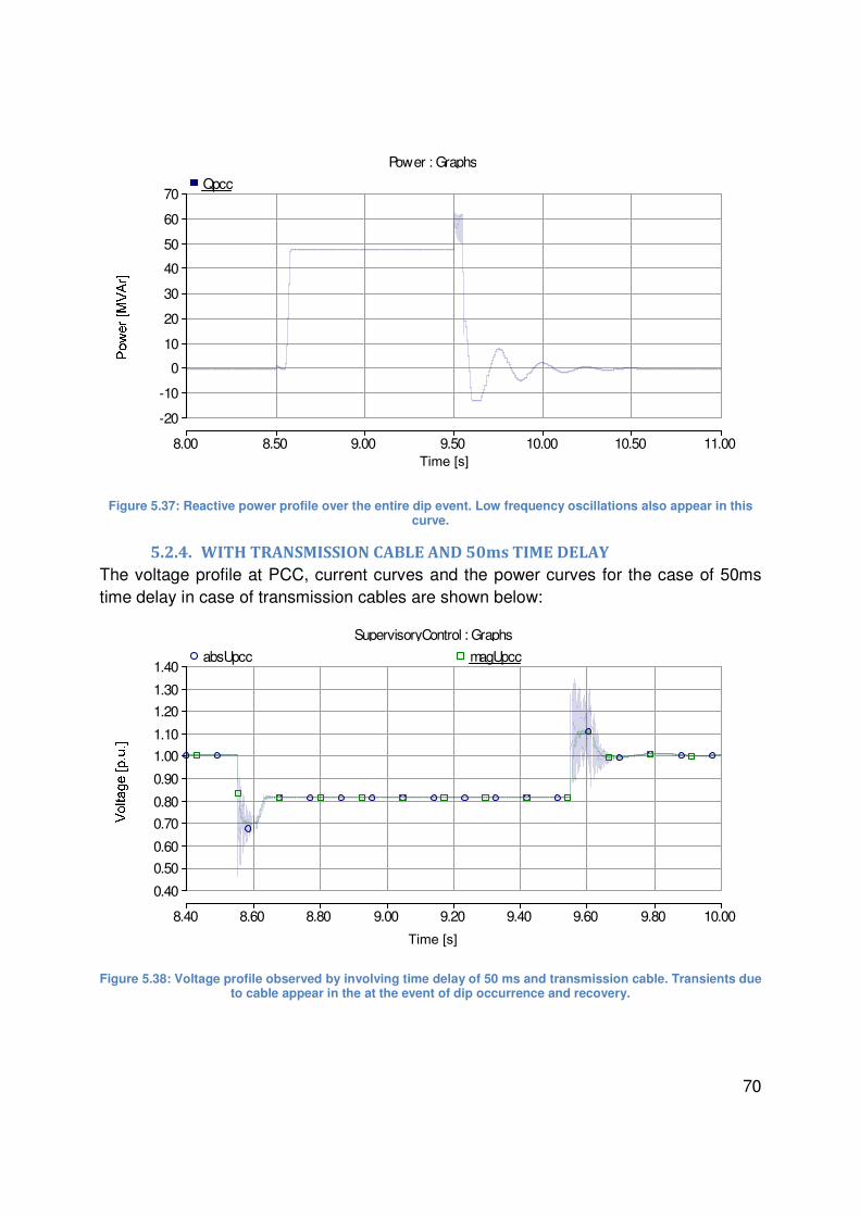
70

Figure 5.37: Reactive power profile over the entire dip event. Low frequency oscillations also appear in this curve.

5.2.4. WITH TRANSMISSION CABLE AND 50ms TIME DELAY

The voltage profile at PCC, current curves and the power curves for the case of 50ms time delay in case of transmission cables are shown below:

Figure 5.38: Voltage profile observed by involving time delay of 50 ms and transmission cable. Transients due to cable appear in the at the event of dip occurrence and recovery.

Power : Graphs

8.00 8.50 9.00 9.50 10.00 10.50 11.00 ... ... ...

-20

-10

0

10

20

30

40

50

60

70

y

Qpcc

Time [s]


8.40 8.60 8.80 9.00 9.20 9.40 9.60 9.80 10.00 ... ... ...

0.40

0.50

0.60

0.70

0.80

0.90

1.00

1.10

1.20

1.30

1.40

y

absUpcc magUpcc

Time [s]

71

Figure 5.39: Reactive current behavior with transmission cable and 50 ms time delay. Low frequency transients also visible within the curves as was the case with Zcable. High frequency transients due to

voltage saturation also visible in the curve.

Figure 5.40: Active current behavior over the entire dip event. During saturation the active current deviates from the reference. 50ms time delay was implemented within the system.


8.25 8.50 8.75 9.00 9.25 9.50 9.75 10.00 10.25 10.50 ... ... ...

-1.40

-1.20

-1.00

-0.80

-0.60

-0.40

-0.20

0.00

0.20

0.40

y

Iq_ref Iq

Time [s]


8.00 8.50 9.00 9.50 10.00 10.50 11.00 ... ... ...

-0.50

-0.25

0.00

0.25

0.50

0.75

1.00

1.25

1.50

y

Id_ref Id absUpcc

Time [s]

72

Figure 5.41: Active power plot along with the reference over the entire dip event. Deviation of active power from the reference during the saturation can be observed here as well. 50ms time delay was implemented.

Figure 5.42: Reactive power simulation over the entire dip event. Low frequency transients due to the phase deviation induced by the delay of 50 ms are easily observed.

It can be concluded from the above figures that the dynamic behavior of the system with the inclusion of delay is similar to the one obtained in the case of only Zcable. The inclusion of cable system has no adverse or better effects on the system in comparison to the system with Zcable. The transients appearing in the system are again due to the energizing and de energizing phenomena discussed in the section of cable system when no delays were included within the system.


8.00 8.50 9.00 9.50 10.00 10.50 11.00 ... ... ...

-40

-30

-20 -10

0

10

20

30

40 50

60

70

y

Pref Ppcc

Time [s]

Power : Graphs

8.25 8.50 8.75 9.00 9.25 9.50 9.75 10.00 10.25 10.50 ... ... ...

-20

-10

0

10

20

30

40

50

60

70

80

y

Qpcc

Time [s]

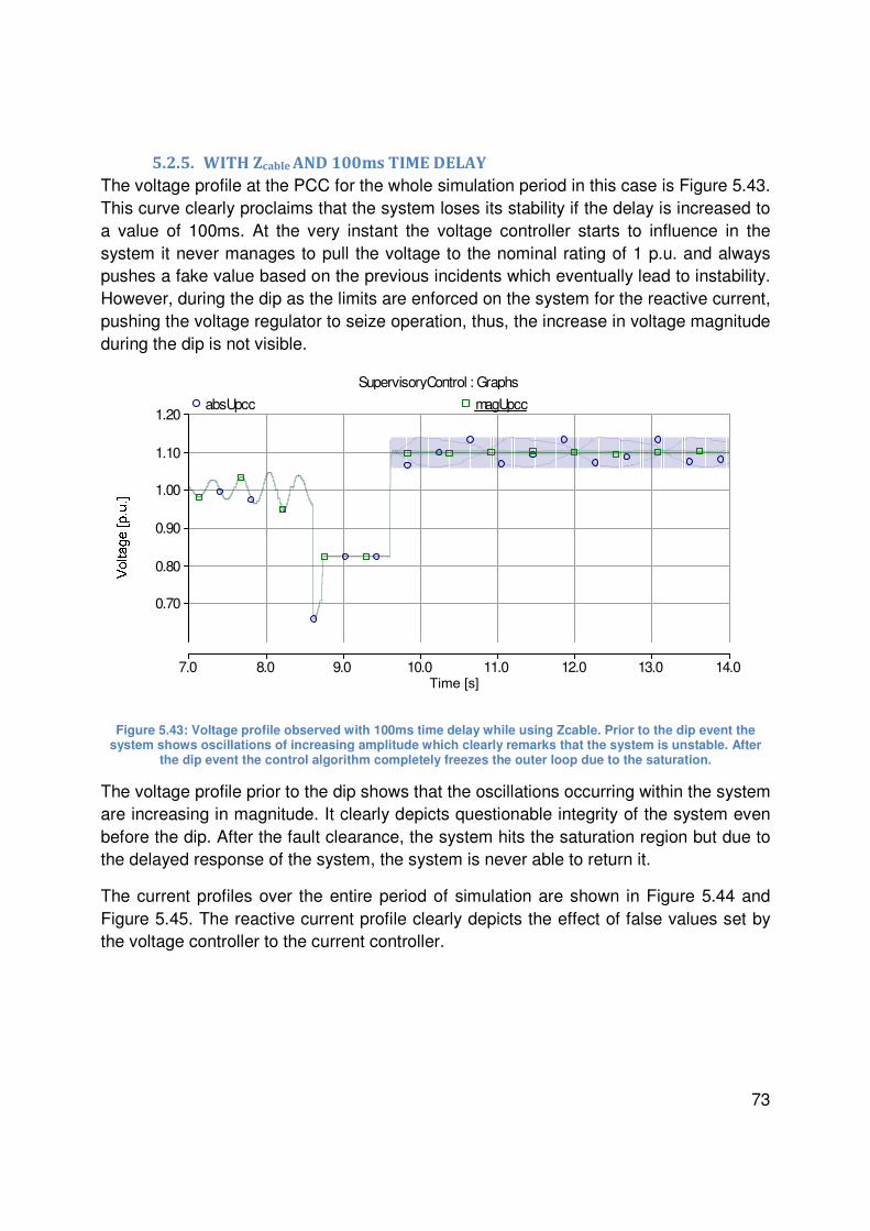
73

5.2.5. WITH Zcable AND 100ms TIME DELAY

The voltage profile at the PCC for the whole simulation period in this case is Figure 5.43. This curve clearly proclaims that the system loses its stability if the delay is increased to a value of 100ms. At the very instant the voltage controller starts to influence in the system it never manages to pull the voltage to the nominal rating of 1 p.u. and always pushes a fake value based on the previous incidents which eventually lead to instability. However, during the dip as the limits are enforced on the system for the reactive current, pushing the voltage regulator to seize operation, thus, the increase in voltage magnitude during the dip is not visible.

Figure 5.43: Voltage profile observed with 100ms time delay while using Zcable. Prior to the dip event the system shows oscillations of increasing amplitude which clearly remarks that the system is unstable. After

the dip event the control algorithm completely freezes the outer loop due to the saturation.

The voltage profile prior to the dip shows that the oscillations occurring within the system are increasing in magnitude. It clearly depicts questionable integrity of the system even before the dip. After the fault clearance, the system hits the saturation region but due to the delayed response of the system, the system is never able to return it.

The current profiles over the entire period of simulation are shown in Figure 5.44 and Figure 5.45. The reactive current profile clearly depicts the effect of false values set by the voltage controller to the current controller.


7.0 8.0 9.0 10.0 11.0 12.0 13.0 14.0 ... ... ...

0.70

0.80

0.90

1.00

1.10

1.20

y

absUpcc magUpcc

Time [s]

74

Figure 5.44: Active current profile over the entire simulation. Due to slower dynamics of the power controller, the low frequency oscillations in the voltage due to the time delay do not impact the power controller.

Figure 5.45: Reactive current behavior over the entire simulation. Oscillation of increasing magnitude prior to the dip event and the operation in the saturation region after the dip event are clearly visible.

The active and reactive power plots recorded over the entire simulation are Figure 5.46 and Figure 5.47. The active power plots clearly demonstrate that due to the variation of voltage the active power also exhibits oscillations of increasing magnitudes although the active power controller is highly damped. The reason for these oscillations is the oscillation in the reference active power provided to the active power controller which is in our system evaluated on the basis the reactive power delivered to the grid.


7.0 8.0 9.0 10.0 11.0 12.0 13.0 14.0 ... ... ...

-1.00

-0.75

-0.50

-0.25

0.00

0.25

0.50

0.75

1.00

1.25

y

Id_ref Id

Time [s]


7.0 8.0 9.0 10.0 11.0 12.0 13.0 14.0 ... ... ...

-1.75

-1.50

-1.25

-1.00

-0.75

-0.50

-0.25

0.00

0.25

0.50

0.75

y

Iq_ref Iq

Time [s]

75

By varying the time delay in steps of 10ms it was observed that the system manages to remain stable up to 80ms of time delay. At 80ms the system was observed to be marginally stable and above values of delay time push the system to complete unstable region.

Figure 5.46: Oscillations appear in the active power plots prior to the dip event. After the dip event the system fails to recover due to the.

Figure 5.47: Reactive power plot over the entire simulation with oscillations of rising magnitude and fault condition after the fault clearance.


7.0 8.0 9.0 10.0 11.0 12.0 13.0 14.0 ... ... ...

-60

-40

-20

0

20

40

60

y

Pref Ppcc

Time [s]

Power : Graphs

7.0 8.0 9.0 10.0 11.0 12.0 13.0 14.0 ... ... ...

-30

-20

-10

0

10

20

30

40

50

60

70

y

Qpcc

Time [s]

76


The voltage, current and power plots for the system with transmission cables are shown below. The curves depict that the situation of the voltage instability only becomes worst when the cables are utilized. It was observed as the control system fails to provide an appropriate amount of reactive power during the dip scenario therefore the inner loop moves into the saturation region for a limited time, which as a result decreases the amount of uncontrolled active current flowing within the system during this duration.

Figure 5.48: Voltage profile at PCC with 100ms delay and using transmission cable system. Oscillations of increasing magnitude are prominent before the dip event. Saturation of controllers during the dip also

observable.

Figure 5.49: Reactive current profile over the entire simulation with increasing oscillations before the dip and uncontrolled behavior after the fault clearance. Time delay of 100ms was implemented for these curves.


7.0 8.0 9.0 10.0 11.0 12.0 13.0 14.0 ... ... ...

0.40

0.50

0.60

0.70

0.80

0.90

1.00

1.10

1.20

1.30

1.40

y

absUpcc magUpcc

Time [s]


7.0 8.0 9.0 10.0 11.0 12.0 13.0 14.0 ... ... ...

-2.50

-2.00

-1.50

-1.00

-0.50

0.00

0.50

1.00

y

Iq_ref Iq

Time [s]

77

Figure 5.50: Active current profile over the entire simulation. The current fails to follow the reference after the fault clearance. Slower dynamics of power controller keep the active current controller prior to the dip event.

Figure 5.51: Active power profile over the entire simulation showing small oscillations in the reference which as a result are followed by the Power transferred over the PCC as well. This behavior was observed due to the

dependence of reference power on the voltage magnitude.


7.0 8.0 9.0 10.0 11.0 12.0 13.0 14.0 ... ... ...

-2.50

-2.00

-1.50

-1.00

-0.50

0.00

0.50

1.00

1.50

y

Id_ref Id absUpcc

Time [s]


7.0 8.0 9.0 10.0 11.0 12.0 13.0 14.0 ... ... ...

-125

-100

-75

-50

-25

0

25

50

75

y

Pref Ppcc

Time [s]

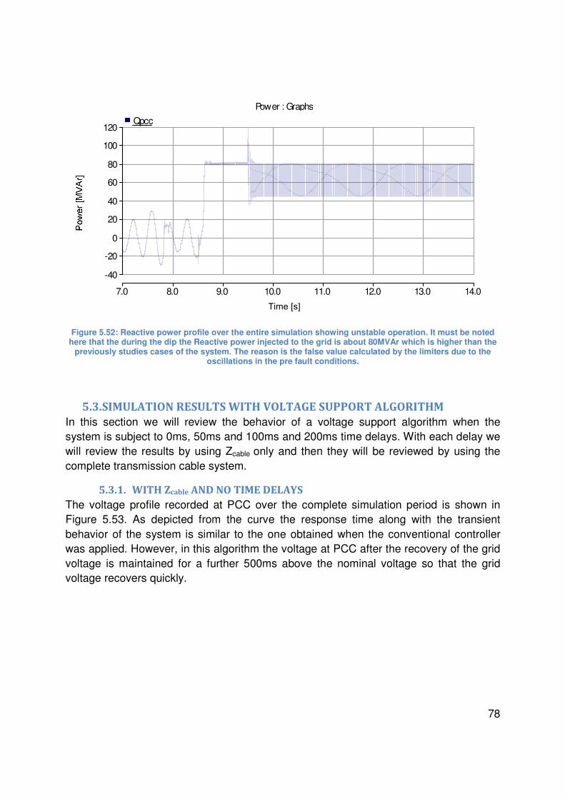
78

Figure 5.52: Reactive power profile over the entire simulation showing unstable operation. It must be noted here that the during the dip the Reactive power injected to the grid is about 80MVAr which is higher than the

previously studies cases of the system. The reason is the false value calculated by the limiters due to the oscillations in the pre fault conditions.

5.3. SIMULATION RESULTS WITH VOLTAGE SUPPORT ALGORITHM

In this section we will review the behavior of a voltage support algorithm when the system is subject to 0ms, 50ms and 100ms and 200ms time delays. With each delay we will review the results by using Zcable only and then they will be reviewed by using the complete transmission cable system.

5.3.1. WITH Zcable AND NO TIME DELAYS

The voltage profile recorded at PCC over the complete simulation period is shown in Figure 5.53. As depicted from the curve the response time along with the transient behavior of the system is similar to the one obtained when the conventional controller was applied. However, in this algorithm the voltage at PCC after the recovery of the grid voltage is maintained for a further 500ms above the nominal voltage so that the grid voltage recovers quickly.

Power : Graphs

7.0 8.0 9.0 10.0 11.0 12.0 13.0 14.0 ... ... ...

-40

-20

0

20

40

60

80

100

120

y

Qpcc

Time [s]

79

Figure 5.53: Voltage profile with voltage support algorithm. No delays were implemented within the system.

As mentioned earlier in the previous chapters the voltage support algorithm requires the measurement of the pre fault conditions of voltage and the reactive current. These values are shown in Figure 5.54.

Figure 5.54: Prefault values of voltage and Iq recorded by the controller along with filtered PCC voltage for voltage support algorithm.

The voltage support algorithm maintains these values throughout the dip and calculates the difference in the measured voltage at the instant the dip occurs; according to which it injects the reactive current to the grid. This reactive current is then maintained for the


8.00 8.50 9.00 9.50 10.00 10.50 11.00 ... ... ...

0.700

0.750

0.800

0.850

0.900

0.950

1.000

1.050

1.100

y

absUpcc magUpcc

Time [s]


8.00 8.50 9.00 9.50 10.00 10.50 11.00 ... ... ...

-0.20

0.00

0.20

0.40

0.60

0.80

1.00

1.20

y

magUpcc Upccpref Iq_pref

Time [s]

80

remaining dip without considering the dynamics of PCC voltage shown in Figure 5.55. Once the system voltage recovers, the voltage algorithm changes the value of the reactive current to a value where the saturation of the inner controller can be avoided while the system still maintains the overexcited operation.

Figure 5.55 Calculated reactive current and the voltage difference

After 500ms of the post fault overexcited operation the voltage support algorithm considers the system to be in normal condition, thus, the PCC voltage is brought back to the nominal value by a very filter with a response time of 0.1s in order to avoid any oscillations. However, at this moment the algorithm recognizes the voltage to be above the nominal value and thus the wind farm momentarily shift to the under excited operating region. After about 800ms from the event of voltage recovery the voltage support once again measures the grid voltage for the final time to bring the voltage back to nominal reading. This whole operation can be clearly visualized from the reactive current curves shown in Figure 5.56.

The reactive power delivered to the grid during the whole simulation period in accordance to the voltage support algorithm is shown in Figure 5.57. It can be observed that reactive power never attains a zero value because we only read the voltage at particular instants throughout the simulation period which leads to a certain error in the reactive power even in the nominal operation.


8.00 8.50 9.00 9.50 10.00 10.50 11.00 ... ... ...

-0.10

0.00

0.10

0.20

0.30

0.40

0.50

y

Udiff Iq_inject

Time [s]

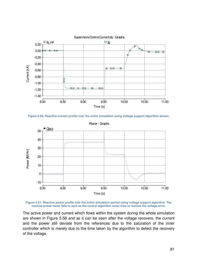
81

Figure 5.56: Reactive current profile over the entire simulation using voltage support algorithm shown.

Figure 5.57: Reactive power profile over the entire simulation period using voltage support algorithm. The reactive power never falls to zero as the control algorithm never tries to remove the voltage error.

The active power and current which flows within the system during the whole simulation are shown in Figure 5.58 and as it can be seen after the voltage recovers, the current and the power still deviate from the references due to the saturation of the inner controller which is merely due to the time taken by the algorithm to detect the recovery of the voltage.


8.00 8.50 9.00 9.50 10.00 10.50 11.00 ... ... ...

-1.40

-1.20

-1.00

-0.80

-0.60

-0.40

-0.20

0.00

0.20

y

Iq_ref Iq

Time [s]

Power : Graphs

8.00 8.50 9.00 9.50 10.00 10.50 11.00 ... ... ...

-10

0

10

20

30

40

50

y

Qpcc

Time [s]

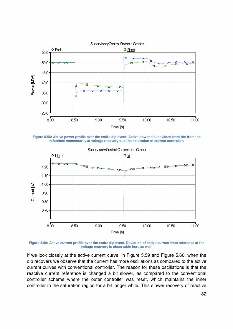
82

Figure 5.58: Active power profile over the entire dip event. Active power still deviates from the from the reference momentarily at voltage recovery due the saturation of current controller.

Figure 5.59: Active current profile over the entire dip event. Deviation of active current from reference at the voltage recovery is observable here as well.

If we look closely at the active current curve, in Figure 5.59 and Figure 5.60, when the dip recovers we observe that the current has more oscillations as compared to the active current curves with conventional controller. The reason for these oscillations is that the reactive current reference is changed a bit slower, as compared to the conventional controller scheme where the outer controller was reset, which maintains the inner controller in the saturation region for a bit longer while. This slower recovery of reactive


8.00 8.50 9.00 9.50 10.00 10.50 11.00 ... ... ...

25.0

30.0

35.0

40.0

45.0

50.0

55.0

y

Pref Ppcc

Time [s]


8.00 8.50 9.00 9.50 10.00 10.50 11.00 ... ... ...

0.70

0.80

0.90

1.00

1.10

1.20

y

Id_ref Id

Time [s]

83

current can be observed in Figure 5.61. The active current is therefore also noticed to have a bit large decrease in magnitude in comparison to the case of conventional voltage controller.

Figure 5.60: Active current profile when the voltage recovers. The current has more oscillations as compared to the active current curves with conventional controller

Voltage support algorithm helps us to deviate from a closed loop operation to an open loop operation where we do not have to rely on the instantaneous voltage conditions during the fault scenarios while being quick in response.

Figure 5.61: Reactive current profile when the voltage recovers. It is observable that the reactive current changes a bit slower as was in the case of conventional controller.


9.440 9.460 9.480 9.500 9.520 9.540 9.560 9.580 9.600 9.620 ... ... ...

0.70

0.80

0.90

1.00

1.10

1.20

y

Id_ref Id

Time [s]


9.480 9.500 9.520 9.540 9.560 9.580 9.600 9.620 9.640 ... ... ...

-1.30

-1.20

-1.10

-1.00

-0.90

-0.80

-0.70

-0.60

-0.50

-0.40

y

Iq_ref Iq

Time [s]

84

5.3.2. WITH TRANSMISSION CABLE AND NO TIME DELAY

The voltage profile recorded at the PCC over the whole simulation period in this case is shown in Figure 5.62:

Figure 5.62: Voltage profile over the entire dip event using transmission cable and voltage support algorithm.

It was observed that with transmission cables the deviation of voltage from the nominal value is still small but is larger than the one observed in the case of the simulations executed with Zcable. The reason behind this problem is the capacitive effect of the cables which store energy and require a constant amount of regulation at PCC to be compensated. This can be visualized from the evaluated reactive current curves shown in Figure 5.63:

Figure 5.63: Evaluated difference and reactive power to be injected when using transmission cables with voltage support algorithm.


8.00 8.50 9.00 9.50 10.00 10.50 11.00 ... ... ...

0.40

0.50

0.60

0.70

0.80

0.90

1.00

1.10

1.20

1.30

1.40

y

absUpcc magUpcc

Time [s]


8.00 8.50 9.00 9.50 10.00 10.50 11.00 ... ... ...

-0.10

0.00

0.10

0.20

0.30

0.40

0.50

y

Udiff Iq_inject

Time [s]

85

At system start up when the algorithm evaluates the reactive current the voltage difference is almost zero. Thus the amount of reactive current injected is almost zero and as a result the algorithm fails to compensate for the reactive power generated by the cable which pushes the voltage slightly above the nominal value. The same is observed when the last reading of the voltage to regulate the voltage when the system recovers from the dip i.e. 800ms after the dip recovery. This behavior of the algorithm is more prominent in the reactive power profile shown in Figure 5.64:

Figure 5.64: Reactive power profile observed over the entire simulation. The voltage support algorithm is not able to fully compensate for the reactive power generated by the cable.

The active power and the active current however exhibit similar properties as observed in the case of Zcable and are shown in Figure 5.65 and Figure 5.66:

Figure 5.65: Active current profile over the entire dip event. Deviation of the active current from reference still visible at system voltage recovery.

Power : Graphs

8.00 8.50 9.00 9.50 10.00 10.50 11.00 ... ... ...

-20

-10

0

10

20

30

40

50

60

70

y

Qpcc

Time [s]


8.00 8.50 9.00 9.50 10.00 10.50 11.00 ... ... ...

0.40

0.50

0.60

0.70

0.80

0.90

1.00

1.10

1.20

1.30

y

Id_ref Id

Time [s]

86

Figure 5.66: Active power profile over the entire dip event. Same behavior observed as in the case of Zcable.

The transients observed at the beginning of the simulation, at the instant of the dip and at the recovery of the dip are similar to the ones observed in the case of conventional controller having the same motivation.


In the section of conventional controller we observed that the conventional voltage regulator lost its stability at 100ms as the system was never able to respond to the events occurring within the system within an appropriate time. Therefore, in this case we will look at the system stability at the very same conditions. The voltage profile recorded at the PCC for this case is shown in Figure 5.67:

Figure 5.67: Voltage profile over the entire dip event with 100ms delay in the system using voltage support algorithm. The system exhibits stable behavior even with 100ms delay.


8.00 8.50 9.00 9.50 10.00 10.50 11.00 ... ... ...

10

20

30

40

50

60

70

y

Pref Ppcc

Time [s]


8.00 8.50 9.00 9.50 10.00 10.50 11.00 ... ... ...

0.70

0.80

0.90

1.00

1.10

1.20

y

absUpcc magUpcc

Time [s]

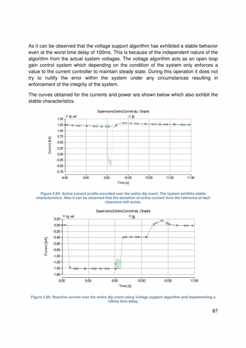
87

As it can be observed that the voltage support algorithm has exhibited a stable behavior even at the worst time delay of 100ms. This is because of the independent nature of the algorithm from the actual system voltages. The voltage algorithm acts as an open loop gain control system which depending on the condition of the system only enforces a value to the current controller to maintain steady state. During this operation it does not try to nullify the error within the system under any circumstances resulting in enforcement of the integrity of the system.

The curves obtained for the currents and power are shown below which also exhibit the stable characteristics.

Figure 5.68: Active current profile recorded over the entire dip event. The system exhibits stable characteristics. Also it can be observed that the deviation of active current from the reference at fault

clearance still exists.

Figure 5.69: Reactive current over the entire dip event using Voltage support algorithm and implementing a 100ms time delay.


8.50 9.00 9.50 10.00 10.50 11.00 11.50 ... ... ...

-0.75

-0.50

-0.25

0.00

0.25

0.50

0.75

1.00

1.25

1.50

y

Id_ref Id

Time [s]


8.50 9.00 9.50 10.00 10.50 11.00 ... ... ...

-1.60

-1.40

-1.20

-1.00

-0.80

-0.60

-0.40

-0.20

0.00

0.20

y

Iq_ref Iq

Time [s]

88

Figure 5.70: Active power profile over the dip event using Voltage support algorithm and implementing a 100ms time delay.

Figure 5.71: Reactive power profile over the entire dip event using Voltage support algorithm and implementing a 100ms time delay.

The transients obtained at the voltage recovery when the current controller enters into the saturation region are also comparable to the cases observed with conventional voltage controller.

Another interesting factor is the overshoot observed in the power plot when the inner controller retreats from the saturation region. This overshoot is due to the charging of the


8.00 8.50 9.00 9.50 10.00 10.50 11.00 11.50 ... ... ...

-30

-20

-10

0

10

20

30

40

50

60

y

Pref Ppcc

Time [s]

Power : Graphs

8.00 8.50 9.00 9.50 10.00 10.50 11.00 ... ... ...

-10

0

10

20

30

40

50

60

70

y

Qpcc

Time [s]

89

integrator involved in the power controller due to the saturation of the inner controller which due to the large integration area enforces the overshoot.


The PCC voltage, current and power profiles obtained over the entire simulation period for this case are shown below:

Figure 5.72: Voltage profile observed with transmission cable and 100ms delay. The system exhibits stable characteristics throughout the simulation.

Figure 5.73: Active current profile observed with transmission cable and 100ms delay. The system exhibits stable characteristics throughout the simulation.


8.00 8.50 9.00 9.50 10.00 10.50 11.00 ... ... ...

0.40

0.50

0.60

0.70

0.80

0.90

1.00

1.10

1.20

1.30

1.40

y

absUpcc magUpcc

Time [s]


8.00 8.50 9.00 9.50 10.00 10.50 11.00 11.50 ... ... ...

-0.75

-0.50

-0.25

0.00

0.25

0.50

0.75

1.00

1.25

1.50

y

Id_ref Id

Time [s]

90

These plots clearly support the finding in the case discussed in previous section. The controller still exhibits a stable behavior with dynamic properties witnessed in the previous sections.

Figure 5.74: Reactive current profile observed with transmission cable and 100ms delay. The system exhibits stable characteristics throughout the simulation.

Figure 5.75: Active power profile observed with transmission cable and 100ms delay. The system exhibits stable characteristics throughout the simulation.


8.00 8.50 9.00 9.50 10.00 10.50 11.00 11.50 ... ... ...

-1.60

-1.40

-1.20

-1.00

-0.80

-0.60

-0.40

-0.20

0.00

0.20

y

Iq_ref Iq

Time [s]


8.00 8.50 9.00 9.50 10.00 10.50 11.00 ... ... ...

-30

-20

-10

0

10

20

30

40

50

60

70

y

Pref Ppcc

Time [s]

91

Figure 5.76: Reactive power profile observed with transmission cable and 100ms delay. The system exhibits stable characteristics throughout the simulation.


The voltage profile observed over the entire simulation at the PCC is shown in Figure 5.77 and it clearly demonstrates that the voltage support algorithm still manages to keep the integrity of the system intact. The current and power plots also support the same findings.

Figure 5.77: Voltage profile observed over the entire dip event with 200ms delay. The system still operates with stable characteristics clearly showing the better performance of Voltage support algorithm than the

conventional controller when time delays exist within the system.

Power : Graphs

8.00 8.50 9.00 9.50 10.00 10.50 11.00 ... ... ...

-20

-10

0

10

20

30

40

50

60

70

80

y

Qpcc

Time [s]


8.50 9.00 9.50 10.00 10.50 11.00 11.50 ... ... ...

0.70

0.80

0.90

1.00

1.10

1.20

y

absUpcc magUpcc

Time [s]

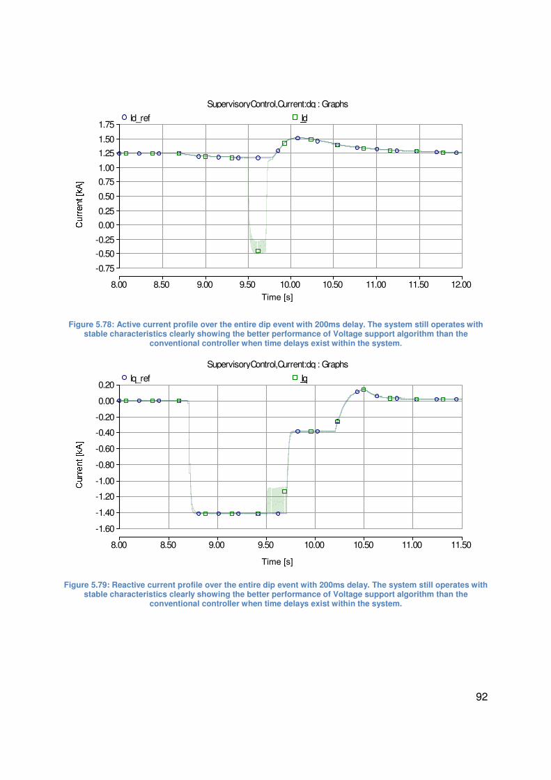
92

Figure 5.78: Active current profile over the entire dip event with 200ms delay. The system still operates with stable characteristics clearly showing the better performance of Voltage support algorithm than the


Figure 5.79: Reactive current profile over the entire dip event with 200ms delay. The system still operates with stable characteristics clearly showing the better performance of Voltage support algorithm than the



8.00 8.50 9.00 9.50 10.00 10.50 11.00 11.50 12.00 ... ... ...

-0.75

-0.50

-0.25

0.00

0.25

0.50

0.75

1.00

1.25

1.50

1.75

y

Id_ref Id

Time [s]


8.00 8.50 9.00 9.50 10.00 10.50 11.00 11.50 ... ... ...

-1.60

-1.40

-1.20

-1.00

-0.80

-0.60

-0.40

-0.20

0.00

0.20

y

Iq_ref Iq

Time [s]

93

Figure 5.80: Active power profile over the entire dip event with 200ms delay. The system still operates with stable characteristics clearly showing the better performance of Voltage support algorithm than the


Figure 5.81: Reactive power profile over the entire dip event with 200ms delay. The system still operates with stable characteristics clearly showing the better performance of Voltage support algorithm than the



The plots obtained for this case were also observed to exhibit the same properties as discussed previously and are shown below:


8.00 8.50 9.00 9.50 10.00 10.50 11.00 11.50 12.00 12.50 ... ... ...

-30

-20

-10

0

10

20

30

40

50

60

70

y

Pref Ppcc

Time [s]

Power : Graphs

8.00 8.50 9.00 9.50 10.00 10.50 11.00 11.50 ... ... ...

-10

0

10

20

30

40

50

60

70

y

Qpcc

Time [s]

94

Figure 5.82: Voltage profile over the entire dip event with 200ms delay and using cables. The system still operates with stable characteristics clearly showing the better performance of Voltage support algorithm than

the conventional controller when time delays exist within the system.

Figure 5.83: Active current over the entire dip event with 200ms delay and using cables. The system still operates with stable characteristics clearly showing the better performance of Voltage support algorithm than



8.00 8.50 9.00 9.50 10.00 10.50 11.00 11.50 ... ... ...

0.40

0.50

0.60

0.70

0.80

0.90

1.00

1.10

1.20

1.30

1.40

y

absUpcc magUpcc

Time [s]


8.00 8.50 9.00 9.50 10.00 10.50 11.00 11.50 12.00 12.50 13.00 ... ... ...

-1.00

-0.50

0.00

0.50

1.00

1.50

2.00

y

Id_ref Id

Time [s]

95

Figure 5.84: Reactive current over the entire dip event with 200ms delay and using cables. The system still operates with stable characteristics clearly showing the better performance of Voltage support algorithm than


Figure 5.85: Active power over the entire dip event with 200ms delay and using cables. The system still operates with stable characteristics clearly showing the better performance of Voltage support algorithm than



8.00 8.50 9.00 9.50 10.00 10.50 11.00 11.50 ... ... ...

-1.60

-1.40

-1.20

-1.00

-0.80

-0.60

-0.40

-0.20

0.00

0.20

y

Iq_ref Iq

Time [s]


8.0 9.0 10.0 11.0 12.0 13.0 14.0 ... ... ...

-30

-20

-10

0

10

20

30

40

50

60

70

y

Pref Ppcc

Time [s]

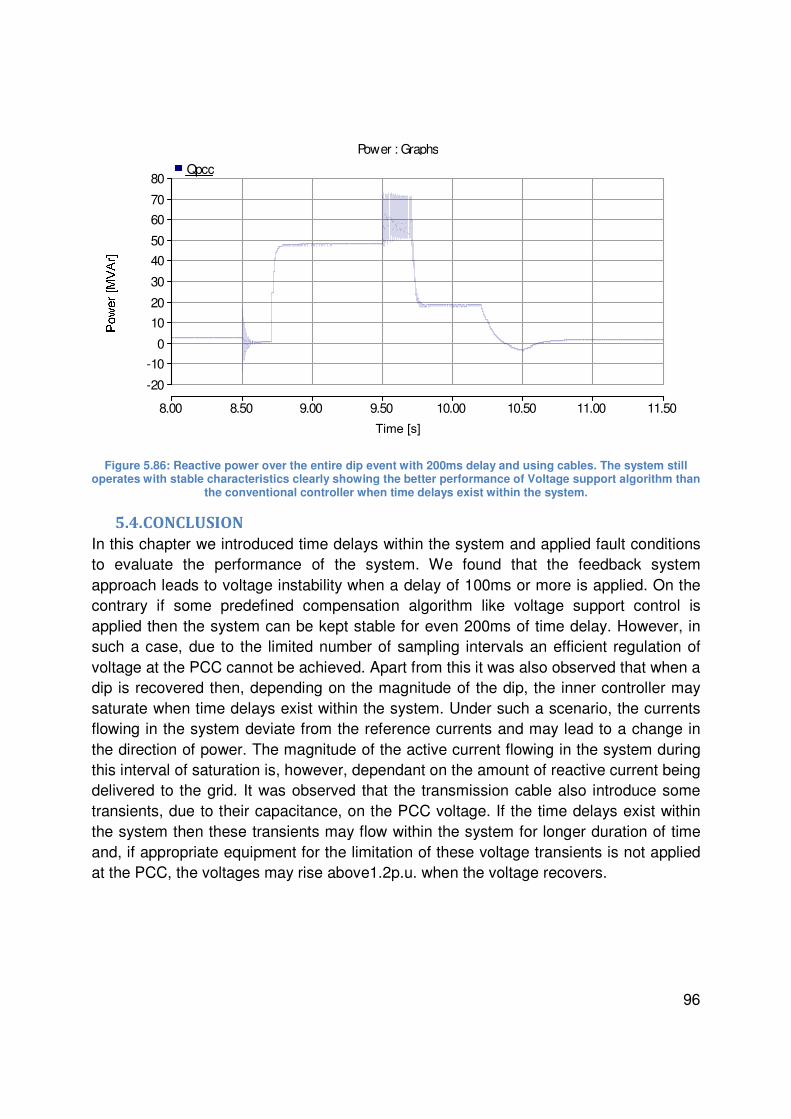
96

Figure 5.86: Reactive power over the entire dip event with 200ms delay and using cables. The system still operates with stable characteristics clearly showing the better performance of Voltage support algorithm than


5.4. CONCLUSION

In this chapter we introduced time delays within the system and applied fault conditions to evaluate the performance of the system. We found that the feedback system approach leads to voltage instability when a delay of 100ms or more is applied. On the contrary if some predefined compensation algorithm like voltage support control is applied then the system can be kept stable for even 200ms of time delay. However, in such a case, due to the limited number of sampling intervals an efficient regulation of voltage at the PCC cannot be achieved. Apart from this it was also observed that when a dip is recovered then, depending on the magnitude of the dip, the inner controller may saturate when time delays exist within the system. Under such a scenario, the currents flowing in the system deviate from the reference currents and may lead to a change in the direction of power. The magnitude of the active current flowing in the system during this interval of saturation is, however, dependant on the amount of reactive current being delivered to the grid. It was observed that the transmission cable also introduce some transients, due to their capacitance, on the PCC voltage. If the time delays exist within the system then these transients may flow within the system for longer duration of time and, if appropriate equipment for the limitation of these voltage transients is not applied at the PCC, the voltages may rise above1.2p.u. when the voltage recovers.

Power : Graphs

8.00 8.50 9.00 9.50 10.00 10.50 11.00 11.50 ... ... ...

-20

-10

0

10

20

30

40

50

60

70

80

y

Qpcc

Time [s]

97

6. CONCLUSION AND FUTURE WORK

This thesis focuses on the influence of time delays exhibited on the performance of a full power converter based wind farms. In this regard, the voltage regulators used for the reactive power compensation along with the voltage support algorithm presented by E.ON grid codes were investigated.

In order to study the behavior of the system, the grid side converter of a wind farm is modeled in PSCAD/EMTDC software. The cascaded control of the grid side converter is based on amplitude invariant and voltage oriented synchronous frame of reference, with an inner current controller and outer voltage and active power controllers. The reactive power control of the system is simplified by changing the IGBT switches and DC link capacitor with DC switches while the DC link voltage controller with an active power controller. The reactive power is controlled by means of voltage control strategies.

The results of this thesis are presented in chapter 5, where the impact of time delays on the dynamic performance of the system during voltage dips is discussed. The results were initially established on time delays of 0, 50ms and 100ms for the droop based voltage regulation scheme. Then, they were acquired on the basis of voltage support algorithm. Apart from this the results presented were acquired either by using a transmission cable or an inductive impedance of the cable neglecting the capacitance.

It can be concluded from the results of this thesis that:

• Time delays in the feedback loop result in voltage instability if they are of more than 80ms.

• Depending on the magnitude of the remaining voltage during a dip, the current controller may enter saturation region when a dip is recovered. The time to remain within this saturation region is decided by the time delay which exists within the system.

• The operation in the saturation region on voltage recovery leads to over voltages if transmission cables are used. Therefore, some protection equipments should be deployed. It was also found that during this operation, the active current largely deviates from the reference current with sharp rate of change.

• In order to make the system stable either the voltage regulator should be made slower in response or the open loop approach should be utilized. However, slow response of voltage regulator is undesired by the grid operators.

• Voltage support algorithm was utilized as an open loop approach and was found that the system regains stability for delays above 80ms. In this context delays up to 200ms were applied and the system was still found to be stable.

• The open loop approach does influence the stability of the system but it fails to avoid the system from entering the saturation region at the voltage recovery.

98

Thus, it fails to avoid over voltages, in case of transmission cables only, and the active current deviation from reference current.

From the above discussion it is clear that whether the system operates as a closed loop or an open loop, yet it fails to maintain control over the current at the incident of voltage recovery. This effects the performance of the system as it leads to deviation of the output current from the reference currents set by the power and voltage control systems making the whole control system sluggish in response. Delay compensation strategies like Smith predictors should be applied to re-evaluate the performance of the system. The idea of such compensation is to use a controller structure which takes the delay out of the control loop and allows a feedback design based on ideal transfer function. A Smith predictor in this way can predict the current output voltage and make the response of the system aggressive as required by the grid codes. Therefore, it is proposed that as a future extension to this thesis a Smith predictor should be applied to enhance the performance of the system.

99

APPENDIX-A: TRANSFORMER DATA

The transformer utilized for these simulations was based on the UMEC approach. However, the core geometry required for designing the transformer was taken as the default values specified in PSCAD. It should also be mentioned here that the Model saturation was turned off during the whole simulations as the aim was not to observe the dynamics of the system due to the saturation of the transformer. Therefore, the major settings applied to the selected transformer are specified in the table below:

Data Configuration

Transformer core construction Five-Limb

Transformer MVA 100.0

Primary Voltage (line-line, rms) 33 kV

Secondary Voltage (line-line, rms) 33 kV

Winding # 1 Type Y

Winding # 2 Type Delta

Delta Lags or Leads Y Lags

Base operation frequency 50.0 Hz

Leakage Reactance 0.12 p.u.

No Load Losses 0.0 p.u.

Copper Losses 0.05 p.u.

Model Saturation No

Tap changer Winding None

Table 1: Transformer Data

Figure A.0.1: UMEC Transformer model used from PSCAD Library

A

B

C

A

B

C

#2#1

33.0 [kV]33.0 [kV]

100.0 [MVA]umec

100

APPENDIX-B: TRANSMISSION CABLE DATA

According to the selected ratings of the system a 30kV, 1200mm2 XLPE cable was selected from the ABB XLPE cable systems User’s guide[15]. The details of the complete cable system are shown below:

Cable Type Single Core

Formation trefoil

Nominal Voltage (rms) 30 kV

Nominal phase current of the system (rms) 1.75 kA

Conductor Cross-Section 1200 mm2

Diameter of Conductor 44.0 mm

Insulation Thickness 8.0 mm

Diameter over Insulation 64.0 mm

Cross-section of screen 35.0 mm2

Outer Diameter of Cable 74.0 mm

Cable Weight (Copper conductor) 14.2 kg/m

Capacitance 0.48 µF/km

Charging current per phase at 50Hz 2.6 A/km

Inductance (trefoil formation) 0.29 mH/km

Surge Impedance 10.1 Ω

Bonding Type Both Ends

Current Rating at 900C 915 A

Number of Cables per phase for desired current 3

Laying Type Underground

Laying Depth 1.0 m Table 2: Cable data selected from ABB Catalog

As depicted from the above table, the selected cable only carries 915 A at the mentioned temperature. Thus, two cables per phase are atleast required to transmit the rated current of 1.75kA. However, in practical systems, the cables are usually designed to be loaded to 70%. Therefore, three cables per phase or three groups of cables were used. It should, however, be remembered that the current carrying capacity is dependent on the number of cable groups deployed and the distance between the cable groups. In our case, two cable groups were parted by 2m which reduces the current carrying capacity to 93%. Then the cable loading and the actual current carrying capacity of the designed cable system is shown in Table 3.

PSCAD MODELING:

In PSCAD, the cable can be designed either by using the cable geometry or by using equivalent pi-section model. The pi-section model is the simplest representation of the cable line and utilizes the cable lumped parameters. However, the pi models do not

101

provide an accurate cable frequency spectrum and are only acceptable for short distances because the error becomes noticeable when the cable length increases. Thus, this model is avoided for transient simulations.

Number of Cable groups 3

Distance between two consecutive groups 2 m

Rating factor for group of cables 0.93

Nominal phase current of cable system designed 2.553 kA

Cable Loading 68.6 % Table 3: Current rating of the selected cable system and their loading at the rated operation

On the contrary, cable designing by cable geometry gives the privilege to model the cable by distributed parameters. Distributed parameter models are further divided into two groups; the Bergeron model and the frequency dependant models. The Bergeron Model is a constant frequency model and is only recommended for steady state analysis, while the frequency dependant models are based on frequency dependant cable parameters. This frequency dependence is achieved by using cable’s propagation and admittance matrices. The frequency dependant phase model is the most accurate model available at present for the modeling of cables and was therefore utilized in our simulations.

A cable model cannot represent all the details and layers of the cables, thus it is necessary to utilize simplifications and apply corrections to the model. The selected cable was designed in PSCAD as having four layers: Conductor, Insulation, screen and outer Insulation.

Conductor:

The conductor is made up of a series of smaller copper wires and compressed into a cylindrical shape, after which a semi-conducting screen is wrapped around the conductor bundle to smooth it out. Because this screen is a semiconductor, it is almost as if the conductor is effectively thicker for high frequencies, and usually a good approximation is to add the semi-conducting screen to the diameter of the conductor. Then, the radius of the conductor including the semi- conducting layer can be evaluated as:

12 (jNFNGNhe2Fj − 2 ∗ he2FjcℎjNee) This implies,

24

102

The cross-section of the conductor specified in the catalog is not equal to the one obtained from the evaluated conductor radius rc. This difference is used to correct the resistivity, in order to match the DC resistance of the cable, by the following formula:

l m ∗ #

Where, 5E2FNejeFjGjF l 511NNejeFjGjF 1.72 × 10−4Ω. # E2Fee − eNFjjEFeℎNNF This implies,

2.6 × 10OΩ.

Insulation:

Radius of the outer layer of the insulation can be calculated as:

12 (jNFNGNhe2Fj) This implies,

32

The relative permittivity of the insulation should be corrected in order to adjust the capacitance of the cable. The capacitance of the cable can be evaluated as:

5 ]-18. d

Then,

]- 18. 5. ≈ 2.5

Screen:

The data presented in Table 2 demonstrates that the diameter over the screen is not presented to the users. Therefore, the radius over the screen is calculated from the cross-section of the screen, specified by the manufacturer, by the following relation:

103

?#m +8 Where,

As = cross-section of the screen

Then,

32.17

From the above mentioned equation it can be observed that no alteration to the screen radius has been considered or no alteration to the cross-section of the screen was introduced as was done for the conductor. Thus, the DC resistance or the resistivity of the screen is not subjected to any adjustment and is taken to be the standard copper resistivity.

Outer Insulation:

The radius over the outer insulation is considered to be the outer radius of the cable. Therefore,

12 (2FNjNFNFℎN5N) i.e.,

37

The outer Insulation of the cable is usually of PVC as mentioned in the ABB catalog [15]. Therefore, the standard permittivity of PVC i.e. 4.5 was considered for this layer.

The summary of the data obtained from the above equations is shown in Table 4.

Other Cable Parameters:

The inductance is dependent on both the self-coupling and the mutual coupling of the magnetic field. The self-inductance can be defined as:

4 -2m +-8m

At higher frequencies the second term disappears from the equation. Then at higher frequencies:

4 5.754 × 10O

104

The inductance at higher frequencies and the capacitance that determines the surge impedance of the cable as:

$ ?45 10.9Ω

Cable Length 10 km

System frequency 50 Hz

Conductor inner radius 0.0 m

Conductor outer radius 0.024 m

Conductor resistivity 2.6 x 10-4

Ω.m

Conductor relative permeability 1

Insulation outer radius 0.032 m

Insulation permitivity 2.5

Insulation relative permeability 1

Metallic Screen outer radius 0.03217 m

Metallic Screen resistivity 1.72 x 10-4

Ω.m

Metallic Screen realative permeability 1

Outer Insulation outer radius 0.037 m

Outer Insulation permitivity 4.5

Outer Insulation realative permeability 1 Table 4: Summary of the concentric layers obtained for cable modeling

The value obtained for the surge impedance is in close relation to the one mentioned in the cable catalog.

According to the ABB catalog [15], the mutual Inductance between the cables can be evaluated as:

4 0.05 + 0.2 f. e Where,

K = 1 for trefoil formation

s = distance between conductor axes

Then,

e . NO..8 79.7

The inductive reactance of the cable can then be evaluated as:

105

0 2m. 41000Ω

Fitting Parameters:

The frequency domain equations for cable parameters cannot be directly simulated in the time domain, making it necessary to fit these functions to the time domain by means of transfer equations [19]. One of the main problems of cable fitting is that it does not guarantee the passivity of the cable, i.e. it does not guarantee that the cable does not generate any active power. Depending on the simulation conditions, these passivity violations may originate incorrect and unstable simulations [19].

Designing a cable in PSCAD/EMTDC requires the user to set a number of calculation parameters and a correct choice of these values may mean the difference between a stable or unstable simulation. The default values are usually suitable for many simulations.

Traveling Time Interpolation On

Curve Fitting Starting Frequency 0.1 Hz

Curve Fitting End Frequency 1.0 x 105 Hz

Total Number of frequency Increments 1000

Max. order of fitting for Ysurge 30

Max. order of fitting for Propagation Function 30

Max. fitting error for Ysurge 1%

Max. fitting error for prop. Func. 1%

Least Squares Weighting Factors

0 to F0 1

F0 1000

F0 to

Fmax 1

Reflectionless line No Table 5: Fitting parameters selected for the simulation with frequency dependent phase model

However if the default values do not fill the purpose then the guidelines below suggest changes that should be made to the default values in order to avoid unstable simulations[19].

• Travel time Interpolation: If the cable end is reached between time steps, the wave travelling time is interpolated, reducing the error. Should be always on.

• Maximum Order of Fitting for YSurge: The user should verify that the number of poles used in the Fitting function is not equal to the defined number. If equal, the number of poles should be increased, in order to assure that the error is inferior to the desired one.

106

• Maximum Fitting Error for YSurge and Prop. Func.: Last parameters to be changed. If the function is unstable or the number of poles insufficient, the error can be increased.

• Max. Order per Delay Grp. for Prop. Func.: The user should verify that the number of poles used in the Fitting function is not equal to the defined number. If equal, the number of poles should be increased, in order to assure that the error is inferior to the desired one.

The selected fitting parameters for our simulations are shown in table 5.

The choice of the time step is also important for a good simulation. A too large time step can either result in unstable or inaccurate simulations. A common rule of thumb is to select a time step that is 10 times smaller than the smallest wave travelling time in the system. The time step of our simulations was considered to be 5µs.

Bonding of the metallic screens:

The electric power losses in a cable circuit are dependent on the currents flowing in the metallic sheaths of the cables. Therefore, by reducing or eliminating the metallic sheath currents through different methods of bonding, it is possible to increase the load current carrying capacity (ampacity) of the cable circuit. Both ends bonding method was exercised in our simulations.

A system is both ends bonded if the arrangements are such that the cable sheaths provide path for circulating currents at normal conditions. This will cause losses in the screen, which reduce the cable current carrying capacity. These losses are smaller for cables in trefoil formation than in flat formation with separation.

The grounding point for the sheaths is often placed in a box, standing on top of the ground. The distance between the box and the cables is represented by a 10 µH inductance. The grounding resistance for the sheaths, however, was considered to be 0.5 Ω.

Cable connection to phases:

Where multiple single core circuits are laid, care must be taken to ensure how the phases are connected to ensure a balanced current distribution. As discussed in Table 3 we are using three groups of cables. Thus the connection to the phases for each group is shown below.

A

B C

A

C B

A

B C

107

Figure A.2: Cable configuration used in PSCAD

100.0 [ohm*m]Relative Ground Permeability:

Ground Resistivity:1.0

Earth Return Formula: Analytical Approximation

0.024[m]

Cable # 1

.032 [m].03217 [m]

.037 [m]

1 [m]

0 [m]

ConductorInsulator 1

SheathInsulator 2

0.024[m]

Cable # 2

.032 [m].03217 [m]

.037 [m]

1.069 [m]

-0.03985 [m]


SheathInsulator 2

0.024[m]

Cable # 3

.032 [m].03217 [m]

.037 [m]

1.069 [m]

0.03985 [m]


SheathInsulator 2

108

Figure A.3: The complete nine cable system implemented in PSCAD

pcca

pccb

pccc

Ta

Tb

Tc

C1Cable1S1

C2

S2

C3

S3

C1Cable1S1

C2

S2

C3

S3

Cable1C

C1Cable2S1

C2

S2

C3

S3

C1Cable2S1

C2

S2

C3

S3

C1Cable3S1

C2

S2

C3

S3

C1Cable3S1

C2

S2

C3

S3

Cable2C

Cable3C

0.00001 [H]

0.00001 [H]

0.00001 [H]

0.00001 [H]

0.00001 [H]

0.00001 [H]

0.00001 [H]

0.00001 [H]

0.00001 [H]

0.00001 [H]

0.00001 [H]

0.00001 [H]

0.00001 [H]

0.00001 [H]

0.00001 [H]

0.00001 [H]

0.00001 [H]

0.00001 [H]

0.5

[oh

m]

0.5

[oh

m]

0.5

[oh

m]

0.5

[oh

m]

0.5

[oh

m]

0.5

[oh

m]

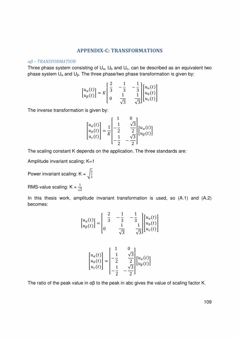
109

APPENDIX-C: TRANSFORMATIONS

αβ – TRANSFORMATION

Three phase system consisting of Ua, Ub and Uc, can be described as an equivalent two phase system Uα and Uβ. The three phase/two phase transformation is given by:

2H(F)2I(F) f ¡ 23− 13 − 130 1√3 1√3¢£

£¤ ¥2!(F)2 (F)2(F)¦ The inverse transformation is given by:

¥2!(F)2 (F)2(F)¦ 1f ¡ 10−12√32−12− √32 ¢£

££¤ 2H(F)2I(F)

The scaling constant K depends on the application. The three standards are:

Amplitude invariant scaling: K=1

Power invariant scaling: K = ;u8 RMS-value scaling: K =

√8 In this thesis work, amplitude invariant transformation is used, so (A.1) and (A.2) becomes:

2H(F)2I(F) ¡ 23− 13 − 130 1√3 1√3¢£

£¤ ¥2!(F)2 (F)2(F)¦

¥2!(F)2 (F)2(F)¦ ¡ 10−12√32−12− √32 ¢£

££¤ 2H(F)2I(F)

The ratio of the peak value in αβ to the peak in abc gives the value of scaling factor K.

110

dq - TRANSFORMATION

In the αβ plane, the vector rotates with angular frequency of L(F) in positive direction for positive three phase system. While in dq plane, the coordinate system rotates with angular frequency of L(F) in the positive direction and the voltage component remains constant, which gives easier analysis and control of the system and determine of the transients.

Figure: voltage vector at time t and t+dt

The transformation from positive sequence αβ to dq and the inverse can be written as:

§2+g(F)2+J(F)¨ ©cos M sin M>sin M cos Mª 2H<F=2I<F=

2H<F=2I<F= ©cos M >sin Msin M cos Mª §2+g<F=2+J<F=¨

The instantaneous active and reactive power can be written as:

2!j!D2 j D2j o 1

√3 2!<j > j = D 2 <j! > j=D2<j > j!=~ Amplitude invariant transformation from abc to dq, we get

32 W2+j+ D 2JjJX

o 32 W>2+jJ D 2Jj+X

111

7. BIBLIOGRAPHY

[1] Francisco Varela, "Plugging the gap: A survey of world fuel resources and its impact on the development of wind energy," Renewable Energy Sytems Limited and Global Wind Energy Council, 2006.

[2] Global Wind Energy Council. (2011, April) GWEC. [Online]. http://gwec.net/fileadmin/images/Publications/GWEC_annual_market_update_2010_-_2nd_edition_April_2011.pdf

[3] Thomas Ackermann, "Historical Development and Current Status of Wind Power," in Wind power in power systems, Thomas Ackermann, Ed.: John Wiley & Sons, Ltd, 2005, ch. 2.

[4] Anca D. Hansen, "Generators and Power Electronics for Wind Turbines," in Wind

power in power systems, Thomas Ackermann, Ed.: John Wiley & Sons, Ltd, 2005, ch. 4.

[5] Olimpo Anaya-Lara, Nick Jenkins, Janaka Ekanayake, Phill Cartwright, and Mike Hughes, Wind energy generation : modelling and control.: John Wiley & Sons Ltd, 2009.

[6] J. G. Slootweg and W. L. Kling, "Impacts of Wind Power on Power System Dynamics," in Wind power in power systems, Thomas Ackermann, Ed.: John Wiley & Sons, Ltd, 2005, ch. 28.

[7] M. Singh, V. Khadkikar, and A. Chandra, "Grid synchronisation with harmonics and reactive power compensation capability of a permanent magnet synchronous generator-based variable speed wind energy conversion system," IET Power

Electronics, vol. 4, no. 1, pp. 122-130, January 2011.

[8] Jan Svensson, "Grid-Connected Voltage Source Converter - Control Principles and Wind Energy Applications," Chalmers University of Technology, Gothenberg, Sweden, PhD Thesis 91-7197-610-8, 1998.

[9] Ned Mohan, Tore M. Udeland, and William P. Robbins, Power Electronics:

Converters, Applications and Design, 2nd ed.: John Wiley and Sons, Ltd, 1995.

[10] P. Channegowda and V. John, "Filter Optimization for Grid Interactive Voltage Source Inverters ," IEEE Transactions on Industrial Electronics , vol. 57, no. 12, pp. 4106-4114, December 2010.

112

[11] S.V. Araujo, A. Engler, B. Sahan, and F. Antunes, "LCL filter design for grid-connected NPC inverters in offshore wind turbines," in ICPE '07. 7th Internatonal

Conference on Power Electronics., October 2007, pp. 1133-1138.

[12] H. L. Thanawala, D. J. Young, and M. H. Baker, "Shunt Compensation: SVC and STATCOM," in Flexible AC Transmission Systems (FACTS), Yong Hua Song and Allan T Johns, Eds. United Kingdom/London: The Institute of Electrical Engineers, 1999, ch. 4.

[13] ABB AB. (2010, April) It's time to connect with offshore wind supplement. [Online]. http://www05.abb.com/global/scot/scot221.nsf/veritydisplay/fb4d15b402dc68c7c12577210040f853/$file/pow0038%20r6%20lr.pdf

[14] EON Netz GmbH, Beyreuth. (2008, April) Requirements for Offshore Grid Connections in the E.ON Netz Network. [Online]. http://www.eon.com/en.html

[15] ABB AB. (2010, April) XLPE Land Cable Systems User's Guide. [Online]. http://www05.abb.com/global/scot/scot245.nsf/veritydisplay/ab02245fb5b5ec41c12575c4004a76d0/$file/xlpe%20land%20cable%20systems%202gm5007gb%20rev%205.pdf

[16] Özgür Salih MUTLU, "Evaluating the Impacts of Wind Farms on Power System Operation," Naval Science and Engineering, vol. 6, no. 2, pp. 166-185, 2010.

[17] P. Kundur, Power System Stability and Control, Neal J. Balu and Mark G. Lauby, Eds.: McGraw-Hill, Inc.

[18] H. Bludszuweit, J.A. Domínguez, and M. García, "The impact of induction generator and PWM Inverter with energy storage on weak grids," in International

Conference on Renewable Energies and Power Quality, 2006.

[19] Filipe Miguel Faria da Silva, "Analysis and simulation of electromagnetic transients in HVAC cable transmission grids," Aalborg University, Denmark, PhD Thesis 2011.

[20] G.C. Tarnowski and R. Reginatto, "Adding Active Power Regulation to Wind Farms with Variable Speed Induction Generators ," in Power Engineering Society General

Meeting, 2007. IEEE, 2007, pp. 1-8.

[21] Amirnaser Yazdani and Reza Iravani, Voltage-sourced converters in power

systems : modeling, control, and applications.: John Wiley & Sons, Inc., 2010.

113

[22] Massimo Bongiorno, "On Control of Grid-connected Voltage Source Converters: Mitigation of Voltage Dips and Subsynchronous Resonances," Chalmers University of Technology, Gothenberg, Sweden, PhD Thesis 978-91-7291-985-3, 2007.

[23] Lennart Harnefors, Control of Variable - Speed Drives, 2002, Compendium.

[24] Lidong Zhang, "Modeling and Control of VSC-HVDC Links Connected to Weak AC Systems," Royal Institute of Technology, Sweden, Stockholm, PhD Thesis 978-91-7415-640-9, 2010.

[25] R. Ottersten and J. Svensson, "Vector current controlled voltage source converter-deadbeat control and saturation strategies," IEEE Transactions on Power

Electronics, vol. 17, no. 2, pp. 279-285, March 2002.

[26] A. Luna, P. Rodriguez, R. Teodorescu, and F Blaabjerg, "Low voltage ride through strategies for SCIG wind turbines in distributed power generation systems ," in Power Electronics Specialists Conference, 2008. PESC 2008. IEEE, 2008, pp. 2333 - 2339.

on reactive power compensation of wind farms – impact of wind farm

Documents