On Methods for Real Time Sampling

and Distributions in Sampling

Kadri Meister

Doctoral DissertationDepartment of Mathematical StatisticsUmea UniversitySE-901 87 UmeaSweden

c© 2004 by Kadri MeisterISBN 91-7305-795-9Printed by Print & MediaUmea 2004

Emale

To my mother

Ei joua kirjutada puhtanditme selles elus.Nagu on, nii jaabsee paranduste mitmekordne raga.

? ? ?

No time to write the final draftwithin this lifetime.Leave as it isthe thorny tangled thicket of corrections.

? ? ?

Vi hinner inte med en renskrifthar i livet.Som det var, sa far det varamed alla rattelsers harva.

Doris Kareva

Contents

List of papers viii

Abstract ix

Preface xi

1 Introduction 1

2 Inferential issues 22.1 Basic notation . . . . . . . . . . . . . . . . . . . . . . . . . . . . . 22.2 Different approaches to inference when sampling from a finite po-

pulation . . . . . . . . . . . . . . . . . . . . . . . . . . . . . . . . 42.3 More about some estimators . . . . . . . . . . . . . . . . . . . . . 7

3 Real time sampling situations 83.1 Background . . . . . . . . . . . . . . . . . . . . . . . . . . . . . . 83.2 Suitable sampling methods . . . . . . . . . . . . . . . . . . . . . . 103.3 Comparison of methods . . . . . . . . . . . . . . . . . . . . . . . 123.4 About stationary Bernoulli processes . . . . . . . . . . . . . . . . 13

4 On distributional characteristics in sampling 15

5 Summary of the papers 16Paper A. Some real time sampling methods . . . . . . . . . . . . . . . 16Paper B. Asymptotic considerations concerning real time sampling meth-

ods . . . . . . . . . . . . . . . . . . . . . . . . . . . . . . . . . . . 17Paper C. Some different methods to get stationary Bernoulli sequences

with negative correlations for sampling applications . . . . . . . . 17Paper D. Statistical inference in sampling theory . . . . . . . . . . . . 18Paper E. Sampling design and sample selection through distribution

theory . . . . . . . . . . . . . . . . . . . . . . . . . . . . . . . . . 18Paper F. The design-based distribution of some estimators in survey

sampling . . . . . . . . . . . . . . . . . . . . . . . . . . . . . . . . 18

6 Conclusions and open problems 19

References 21

Papers A–F

vii

List of papers

The present thesis is based on the following papers.

A. Meister, K. and Bondesson, L. (2001). Some real time sampling methods.Research Report 2001–2, Department of Mathematical Statistics, UmeaUniversity. Revised version.

B. Meister, K. (2002). Asymptotic considerations concerning real time samp-ling methods. Statistics in Transition, 5, 1037–1050.

C. Meister, K. (2004). Some different methods to get stationary Bernoulli se-quences with negative correlations for sampling applications. Manuscript.

D. Traat, I., Meister, K. and Sostra, K. (2001). Statistical inference in samplingtheory. Theory of Stochastic Processes, 7, 301–316.

E. Traat, I., Bondesson, L. and Meister, K. (2004). Sampling design and sampleselection through distribution theory. Journal of Statistical Planning andInference, 123, 395–413.

F. Meister, K. and Traat, I. (1999). On the design-based distribution of someestimators in survey sampling. Theory of Stochastic Processes, 3, 324–329.

Papers B, D, E, and F are reprinted with the kind permission of the publishers.

viii

Abstract

This thesis is composed of six papers, all dealing with the issue of sampling from afinite population. We consider two different topics: real time sampling and distri-butions in sampling. The main focus is on Papers A–C, where a somewhat specialsampling situation referred to as real time sampling is studied. Here a finite popu-lation passes or is passed by the sampler. There is no list of the population unitsavailable and for every unit the sampler should decide whether or not to sampleit when he/she meets the unit. We focus on the problem of finding suitable sam-pling methods for the described situation and some new methods are proposed.In all, we try not to sample units close to each other so often, i.e. we sample withnegative dependencies. Here the correlations between the inclusion indicators,called sampling correlations, play an important role. Some evaluation of the newmethods are made by using a simulation study and asymptotic calculations. Westudy new methods mainly in comparison to standard Bernoulli sampling whilehaving the sample mean as an estimator for the population mean. Assuming astationary population model with decreasing autocorrelations, we have found theform for the nearly optimal sampling correlations by using asymptotic calcula-tions. Here some restrictions on the sampling correlations are used. We gainmost in efficiency using methods that give negatively correlated indicator variab-les, such that the correlation sum is small and the sampling correlations are equalfor units up to lag m apart and zero afterwards. Since the proposed methods arebased on sequences of dependent Bernoulli variables, an important part of thestudy is devoted to the problem of how to generate such sequences. The correla-tion structure of these sequences is also studied.

The remainder of the thesis consists of three diverse papers, Papers D–F, wheredistributional properties in survey sampling are considered. In Paper D the con-cern is with unified statistical inference. Here both the model for the populationand the sampling design are taken into account when considering the propertiesof an estimator. In this paper the framework of the sampling design as a multi-variate distribution is used to outline two-phase sampling. In Paper E, we giveprobability functions for different sampling designs such as conditional Poisson,Sampford and Pareto designs. Methods to sample by using the probability func-tion of a sampling design are discussed. Paper F focuses on the design-baseddistributional characteristics of the π-estimator and its variance estimator. Wegive formulae for the higher-order moments and cumulants of the π-estimator.Formulae of the design-based variance of the variance estimator, and covarianceof the π-estimator and its variance estimator are presented.

Key words: Finite population sampling, inferential issues, real time sampling,sequential sampling methods, negative sampling correlations, model-design-basedinference, multivariate Bernoulli and multinomial designs.

2000 Mathematics Subject Classifications: 62D05, 62E15, 60G10.

ix

Preface

PhD-studies are like a roller coaster ride, with eagerness to experience new thingsas well as learn more about ones own limits. However, one never really knowswhere it may lead. Just when you think there is nowhere else to go but down,you are pulled back up and everything is turned around. Occasionally, the ridegives you a butterflies-in-the-stomach feeling but not for long. You are borneaway by negative G-forces that may throw you off if you do not hold on tight.The steepest drop can be several dozen degrees, so to experience the thrills youhave to put up with the screams.

As much as you have enjoyed the intellectual (and emotional) roller coaster ride,you will be relieved when it is all over. In the end, when you look back – withpride – you are going to think it was a great ride! I want to thank the manypassengers in the roller coaster cars for taking this memorable ride with me.

On the first seat, my supervisor Professor Lennart Bondesson. It has beengreat to work with you and take advantage of your broad knowledge and enthu-siasm for solving new problems. I am grateful to you for all helpful discussionsand suggestions. There is still lots more to learn from you about mathematicalstatistics . . . and even more about mushrooms!

Docent Imbi Traat, my co-supervisor at the University of Tartu. Thank you forall the encouragement through the years, and for sharing your ideas and know-ledge, both about statistics and life in general.

Professor Emeritus Gunnar Kulldorff. You have played a central role in thechoice of sampling theory as the topic of my thesis. Thank you for your supportin ’practical matters’ during my first years of studies, and for putting Umea onmy map.

My colleagues at the Department of Mathematical Statistics. You have con-tributed to this work by providing a comfortable and inspiring work atmosphere.Ingrid Westerberg Eriksson and Lennart Nilsson, a special warm thanks forall your help and care!

All current and past (counted from my first visit to Umea) PhD-students. Youhave been a great inspiration for me through all these years! Thank you for sha-ring all the laughs and screams! Special thanks to Mykola for taking one of thephotos on page 9.

Everyone who has commented on and suggested improvements for different partsof this thesis. I am grateful to Paul Haemig for improving my English.

My friends everywhere. For all the enjoyable times we have together! Warmestthanks especially to the ones from Estonia, for always asking when I will be backthere again.

My mother, my brother and his family. Thank you for always being supportiveand understanding, even if you did not fully understand what I was occupied with.

And last but not least, Magnus, on the seat next to me. Thank you for taking allthese roller coaster loops with me! Without you I would never have even thoughtabout going through PhD-studies.

Umea, December 2004Kadri Meister

xi

1 Introduction

We often want to have some information about a specified set of units, a finitepopulation. What is the proportion of unemployed in a country as a whole andin various regions of the country? What is the average expenditure for foodin households? What is the total volume of a forest stand? One way to getanswers to such questions is to collect information from every unit that belongsto the population. Another way is to use some sampling technique. Samplingis choosing in some way just part of a population – called a sample – so thatwith an appropriate study of the sample we may say something about the wholepopulation.

u ee e e u e

e u e e e

u e e e e

e u u e u

e eu e e

e u u u e

e u e ue e

e

u – selected units

e – non-selected units............................................................................................................................

...........................

...................................

............................................................................................................................................................................................................................................................................................................................................................................................................................................................................................................................................................................................................................................................................................................

..........................................................................................................................................................................................

Figure 1: Illustration of a population and a sample

One of the obvious questions here is how to choose the sample. There are manydifferent more or less advanced techniques. As a simple example, we may selectevery 10th unit from the sampling frame – the list of population units. Thesample may be drawn by a probability mechanism, called sampling design. Thelatter then plays a central role by determining how the units are selected fromthe population and also the essential statistical properties of the random quan-tities calculated from the sample. The usual inference problem in sampling is toestimate some summary characteristic of the population, such as the total or themean, after observing the sample. Additionally, we would like to say somethingabout the precision of the estimate, i.e. the size of the sampling error. The latterresults from the fact that the sample is part of the population and estimates fromthe sample may not be identical to the corresponding population quantities. Asampling method that is easy to implement and gives estimates with good preci-sion should be used.

Furthermore, nonsampling errors such as imperfections in the sampling frame,nonresponse, measurement errors, etc., may occur whether the entire populationor a sample of the population is studied and all should be taken into account.

1

Survey sampling theory has a long history. The idea of observing a representativesample instead of the entire population goes back to the late 19th century, andthe work of the Norwegian statistician A. N. Kiær was influential at that time.It is generally agreed that a fundamental step for development of the probabilitysampling approach was made by Neyman (1934). Early developments in theoryand methods concentrated on efficient sampling designs and associated estima-tion techniques for population totals or means. More recently, the methods foranalysis of survey data that take into account the complexity of the samplingdesign – both sampling and nonsampling errors – have developed rapidly.

We will not make any attempt to summarize the history of the subject – thishas already been done by many excellent review papers published in recent years.For a brief history of the development of survey sampling, and in particular theprobability sampling approach, see Hansen, Dalenius & Tepping (1985) and Rao& Bellhouse (1990). Rao (1999) covers some current topics on survey sampling,including developments in survey design, data collection and processing, issuesrelated to inference from survey data, resampling methods for analysis of surveydata, and small area estimation.

This thesis consists of six papers dealing with the issue of sampling from a finitepopulation. Two different topics are treated: real time sampling and distributionsin sampling. In the following sections the theoretical background is given. Sec-tion 2 starts with basic notation and gives definitions used further in the thesis.Then, different approaches to inference when sampling from a finite populationare shortly outlined and some estimators are given. In Section 3, a real time sam-pling situation is described and some suitable sampling methods are presented.In Section 4, we give a brief overview of different problems that form the basefor the work in Papers D–F. In Section 5, the contents of the different papers inthe thesis are summarized. In Section 6, some conclusions are given and openproblems are discussed.

2 Inferential issues

2.1 Basic notation

The fundamental problem in sampling theory is to make inference (estimation,variance estimation, confidence intervals), for example about the population totalby observing a sample selected according to a specified sampling method.

Let U = {1, 2, . . . , N} denote a finite population of N units. Traditionally,there are two distinguished definitions of a sample in the sampling literature

2

(e.g. Sarndal, Swensson & Wretman, 1992, pp. 27–28, 49–50). In the case ofsampling without replacement (WOR) where a unit, once sampled can not besampled again, a sample s is defined as a subset of population U . For samplingwith replacement (WR), where a unit is allowed to be sampled several times, wecan look at the vector of selected units. Here the unit selected at the kth drawis the kth element of the vector. Hence this vector includes information on boththe selecting order of the units and the number of times each unit is selected. Asample s can be defined as the set of distinct units in this vector.

Random selection of a sample s of size n from a finite population U can usuallybe described by some probability mechanism, called sampling design. A samplingdesign p(s) is defined as a probability distribution on sets; p(s) is the probabilityto get the sample (set) s.

The inclusion of a given unit i in a sample is a random event indicated by therandom variable Ii, an inclusion indicator. Here Ii = 0 if unit i is not included inthe sample and Ii = ki, where ki > 0 is some integer, if it is included (ki showsthe number of times unit i is selected). The N indicators can be summarized invector form as I = (I1, I2, . . . , IN). WR-sampling designs are not used so oftenand if not stated otherwise, we have a WOR-design in mind in the remainingdiscussion. In the case of WOR-design, the inclusion indicator Ii takes only thevalues 0 or 1. It is a random variable from a Bernoulli distribution with

E(Ii) = πi, V ar(Ii) = πi(1− πi),

Corr(Ii, Ij) = Rij = (πij − πiπj)/√

πiπj(1− πi)(1− πj), i 6= j,

where πi = Pr(Ii = 1) and πij = Pr(Ii = 1, Ij = 1) are the inclusion probabilitiesof first- and second-order, respectively, and are fundamental characteristics of agiven sampling design.

The sampling design is often chosen to yield certain desired first- and second-orderinclusion probabilities. The estimators used in survey sampling are functions ofthe inclusion indicators, hence the moments of the estimators are functions of thefirst- and higher-order inclusion probabilities, respectively. Knowledge of the πi

and πij alone is normally sufficient for one of the primary goals in survey sam-pling, namely to determine exact or approximate expected values and variancesof the estimators, and to determine variance estimators.

The correlations Rij = Corr(Ii, Ij), here referred to as sampling correlations,are sometimes used instead of πij for describing different sampling designs in thepresent thesis.

3

Let Y = (Y1, Y2, . . . , YN) be the vector of values of the study variable Y for thepopulation units. Sometimes there is some information available about anothervariable X prior to sampling. This variable, called an auxiliary variable, cancarry information about the study variable and hence assist in the estimation.For example, in many surveys of human populations, we can have the value ofthe study variable from a previous census as an auxiliary variable. The goal is toobtain estimators with increased precision for the study variable.

In the following discussion, we use Y (and X) to represent both the variable andthe population total. The exact meaning is given in the context.

There have been some different viewpoints on how to make inference in surveysampling, depending on the source of randomness. The major approaches arebriefly described in the following section.

2.2 Different approaches to inference when sampling froma finite population

Foundational aspects of inference from sample survey data have attracted a lotof attention since the 1960’s.

Finite population sampling is the area of statistics in which the primary mode ofthe analysis is based on the sampling design, the distribution of I, rather thanon statistical models for the variable Y . This is called the design-based approach.Here the population units have fixed but unknown values of the study variableY . The uncertainty in estimates obtained by sampling thus stems from the factthat only part of the population is studied. This means that randomness is onlycoming from the sampling design, i.e. the sole random quantities are the inclusionindicators. While the population characteristic remains fixed, the estimate of itdepends on which sample is selected.

Example 1. An often used estimator for the population total Y is

YHT =∑ IiYi

πi

,

the well-known Horvitz-Thompson estimator (called the HT-estimator or the π-estimator) introduced by Horvitz & Thompson (1952). Here and in the followingdiscussion, any sum

∑without summation restrictions means a sum over the

whole population. Since the values of Yi/πi are given constants, we can easily seethat this estimator is design-unbiased, i.e. Ep(Y ) = Y, where the index p denotesthat the expectation is with respect to the sampling design. Design-unbiasedvariance estimators have been derived by Horvitz & Thompson (1952), Yates &

4

Grundy (1953) and Sen (1953). The goodness of the HT-estimator depends onthe values of πi, working best when πi is approximately proportional to the valueof Yi.

In general, using design-based inference with careful attention to the samplingdesign and using a suitable estimation method, we can obtain estimates that havegood properties without relying on any assumptions about the population itself.

In some sense an opposite approach is the model-based approach, which requiressome probability model ξ for the N -dimensional distribution of Y . Here the po-pulation values Y1, Y2, . . . , YN are random variables, generated by a model ξ, oftencalled a superpopulation model. The specification of ξ can vary from somethingcrude and basic to a very detailed description, depending on what assumptionsthe model maker feels are rational to make. For example, a simple model to adoptis that Y1, Y2, . . . , YN are independent with Eξ(Yi) = µ and V arξ(Yi) = σ2. Theactual finite population values are considered to be realizations of Y1, Y2, . . . , YN

and the inference still concerns the finite population and its parameters.

Example 2. We can write the population total Y as

Y =∑

Yi =∑

i∈s

Yi +∑

i/∈s

Yi.

Here the values of non-selected units are predicted using the model and then asuitable estimator Y is derived. Hence the estimators are dependent on the cho-sen model. Now, however, the properties of the Y , e.g. unbiasedness, are derivedwith respect to the model ξ and not with respect to the sampling design p.

Model-based inference may have advantages if the model is appropriate. Thechallenge with the model-based approach lies in the question of how to specifythe model exactly. The major weakness of the model-based approach is that ifthe model is misspecified, it may lead to invalid conclusions.

Models are widely used also within the design-based inference, both in samplingdesign and in estimation, but in a model-assisted way using the terminology ofSarndal, Swensson & Wretman (1992, p. 227). The values of the study variableare still fixed, but assumptions about a possible model that has generated thesevalues are made. For example, we can assume some correlation structure in themodel. In the case of available auxiliary information, a relation between the studyvariable and the auxiliary variable can be assumed. These assumptions are notexpected to hold exactly.

Example 3. Let Y be some estimator of the population total. We can study howthis estimator behaves under different population models, for example by calcu-

5

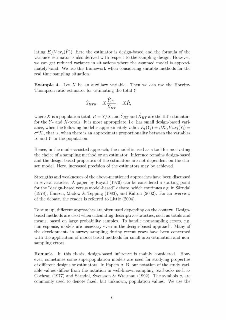
lating Eξ(V arp(Y )). Here the estimator is design-based and the formula of thevariance estimator is also derived with respect to the sampling design. However,we can get reduced variance in situations where the assumed model is approxi-mately valid. We use this framework when considering suitable methods for thereal time sampling situation.

Example 4. Let X be an auxiliary variable. Then we can use the Horvitz-Thompson ratio estimator for estimating the total Y

YHTR = XYHT

XHT

= XR,

where X is a population total, R = Y/X and YHT and XHT are the HT-estimatorsfor the Y - and X-totals. It is most appropriate, i.e. has small design-based vari-ance, when the following model is approximately valid: Eξ(Yi) = βXi, V arξ(Yi) =σ2Xi, that is, when there is an approximate proportionality between the variablesX and Y in the population.

Hence, in the model-assisted approach, the model is used as a tool for motivatingthe choice of a sampling method or an estimator. Inference remains design-basedand the design-based properties of the estimators are not dependent on the cho-sen model. Here, increased precision of the estimators may be achieved.

Strengths and weaknesses of the above-mentioned approaches have been discussedin several articles. A paper by Royall (1970) can be considered a starting pointfor the ”design-based versus model-based” debate, which continues e.g. in Sarndal(1978), Hansen, Madow & Tepping (1983), and Kalton (2002). For an overviewof the debate, the reader is referred to Little (2004).

To sum up, different approaches are often used depending on the context. Design-based methods are used when calculating descriptive statistics, such as totals andmeans, based on large probability samples. To handle nonsampling errors, e.g.nonresponse, models are necessary even in the design-based approach. Many ofthe developments in survey sampling during recent years have been concernedwith the application of model-based methods for small-area estimation and non-sampling errors.

Remark. In this thesis, design-based inference is mainly considered. How-ever, sometimes some superpopulation models are used for studying propertiesof different designs or estimators. In Papers A–B, our notation of the study vari-able values differs from the notation in well-known sampling textbooks such asCochran (1977) and Sarndal, Swensson & Wretman (1992). The symbols yi arecommonly used to denote fixed, but unknown, population values. We use the

6

symbol Yi to denote both the random variable associated with the ith populationunit (if some model is used) and a fixed finite population value. This notation isalso used e.g. in Raj (1968).

2.3 More about some estimators

In this section, the concern is with design-based inference. We assume a samplingdesign that ensures positive first-order inclusion probabilities, πi, and also posi-tive second-order inclusion probabilities, πij, for all i 6= j. Such designs permitdesign-unbiased estimators and variance estimators.

The sample size n, is given by n =∑

Ii. Hence E(n) =∑

πi and

V ar(n) =∑

πi(1− πi) + 2∑ ∑

i<j(πij − πiπj).

Sampling methods that give random sample size are often avoided in practicesince the variable sample size will cause an increase in variance for certain typesof estimators. The double sum in V ar(n) depends on the correlations betweenthe inclusion indicators and it is clear that one must sample with negative de-pendencies in order to get low sample size variation.

Further, we consider estimation of the population mean Y . The Horvitz-Thompsonestimator of Y is

ˆY HT =1

N

∑IiYi =

1

NYHT , (1)

where Yi = Yi/πi, which is the notation introduced in Sarndal, Swensson &Wretman (1992, p. 42). There are different forms for the variance of the HT-estimator. For fixed size sampling designs, it can be given in the Sen-Yates-Grundy form (Sen, 1953; Yates & Grundy, 1953) by

V ar( ˆY HT ) = − 1

2N2

∑ ∑(πij − πiπj)(Yi − Yj)

2

and its unbiased estimator is given by

V ar( ˆY HT ) = − 1

2N2

∑ ∑ πij − πiπj

πij

(Yi − Yj)2IiIj,

where the summation is effectively over the sample.

Since we can view Y as a ratio of two population totals, Y and N , respectively,another possible estimator of Y is

ˆY HTR =YHT

N=

∑IiYi∑Ii

, (2)

7

where Ii = Ii/πi. For πi ≡ π the estimator (2) reduces to the sample mean y.

Since y is a nonlinear function of the inclusion indicators, it has a slight bias. Anapproximate MSE of the estimate y is given by

MSE(y) ≈ − 1

2(E(n))2

∑ ∑aij(Yi − Yj)

2,

where E(n) = Nπ and the coefficients aij = E((Ii − n/N)(Ij − n/N)) are func-tions of the second-order inclusion probabilities.

The estimator ˆY HTR performs better than (1) in cases where the sample size isvariable. Therefore it is used as an estimator for real time sampling methods.

3 Real time sampling situations

In the first half of the thesis, Papers A–C, the concern is with the real time sam-pling situation and the corresponding sampling methods. The sampling situationunder study may have been considered before by others. However, searches inthe sampling literature and databases have not revealed any systematic attentionand research about the underlying case.

3.1 Background

When taking a sample from a finite population, there is often a sampling frameavailable. Units to be measured are selected from the frame by some procedurecorresponding to a chosen sampling design. There are many different methodsto use for this case, depending for example on the amount of accessible auxiliaryinformation.

Consider now a sampling situation where there is no sampling frame availableand where units come, one by one, in real time to a sampler. For every unit thesampler should decide immediately whether or not to sample it by using somesequential selection method. Alternatively, the sampler visits the units in someorder chosen by the sampler. The population size N is usually unknown beforethe sampling but will eventually become known. This kind of sampling is herereferred to as real time sampling.

Example 5. The units may be passengers using the public transportation insome city. It might be possible that the units in the population can order them-selves. In an extreme case, the units can order themselves by taking into account

8

the sampling scheme. Some units, like people coming to a customs control, maywant to avoid being sampled. In such a case, systematic sampling of every fifthunit may be a bad sampling method.

Figure 2: Passengers as sampling units

Example 6. The units may be every tree in a forest stand, with some of thetrees sampled by a forester walking around. The visiting order of the trees in thestand is chosen more or less subjectively by the sampler. Therefore, the selectionof units for the sample is influenced by the sampler’s subjective choice of order.

Figure 3: A forest stand where some trees are sampled

In the following section we present some methods that partly avoid the negativeeffects of ordering.

9

3.2 Suitable sampling methods

As stated before, several well-known sampling methods need a list of the popu-lation and are not suitable to use in real time sampling situations. Here, somesequential selection method is needed. Systematic sampling and Poisson samplingare two possible well-known methods (see e.g. Sarndal, Swensson & Wretman,1992, Chapter 3) to apply for sampling a finite population that passes or is passedby the sampler. Both methods are also easy to use for the sampler.

For systematic sampling in its basic form, the first unit in the sample is drawn bysimple random sampling from among the first µ units in the population. Then,every µth population unit is chosen. However, for systematic sampling there is aproblem with the variance estimator because the condition about positive second-order inclusion probabilities for every pair of units is not fulfilled. This methodis included for comparisons in Paper A but excluded in Papers B and C.

For Poisson sampling, independent U(0, 1) random variables U1, U2, . . . , UN aregenerated to perform the sampling. The selection or non-selection of unit i isdecided by the following rule: if Ui < πi, where πi is a predetermined inclusionprobability, unit i is selected, otherwise not. Because the πis can be specifiedin a variety of ways, Poisson sampling corresponds to a whole class of designs.In the general case, the inclusion probabilities are often chosen to be propor-tional to some size measure. A special case of Poisson sampling is ProbabilityProportional to Prediction (3P) sampling, as described by, for example, Husch,Miller & Beers (2003, p. 355). Here no auxiliary information is accessible priorto sampling and the inclusion probabilities are based on predicted values of thestudy variable. This method is commonly recommended as a sampling methodin forestry, at least in the US. When all the units have the same inclusion prob-ability, πi ≡ π, Poisson sampling is called Bernoulli sampling. Since samplingmethods with equal inclusion probabilities are studied in Papers A–C, just thelatter is considered for comparisons in the following discussion.

For Bernoulli sampling, population units are selected independently of each other.Neighbouring units may have similar study variable values, and therefore it maybe wise not to sample units close to each other too often. Hence sampling withnegative dependencies, i.e. with negative sampling correlations, would be moreefficient. We introduce some sampling methods that partly take into account thepre-history of the sampling.

These methods, as well as Bernoulli sampling, usually give random sample size.However, for sampling methods with negative sampling correlations, the variabil-ity of the sample size is smaller than for Bernoulli sampling.

10

There are several alternative methods with which to perform the sampling. Whenapplying Bernoulli sampling, we sample population units for which the corre-sponding random numbers are below some level. By permitting these randomnumbers to be dependent, two simple extensions of this method are obtained:sampling according to a stationary process and sampling according to some func-tion of independent uniform random variables.

For sampling according to a stationary process, a strictly stationary process {Zi}with given correlations rk = Corr(Zi, Zi+k) is used as a tool for defining thevalues of the inclusion indicators. We set

Ii ={

1 if Zi ≤ c0 otherwise

,

where c is a given constant determined by the desired inclusion probability π, i.e.c = F−1(π), where F is the distribution function of Zi. The process {Zi} must beeasy to simulate, so a stationary standard normal process is mainly considered,both in Papers A and C.

Sampling according to some function of independent uniform random variablesis introduced in Paper C. We generate independent U(0, 1) random variablesU1−m, U2−m, U3−m, . . ., where m ≥ 1 is some fixed integer. The general rule fordefining the value of Ii is

Ii ={

1 if Ui ≤ h(Ui−m, . . . , Ui−2, Ui−1)0 otherwise

,

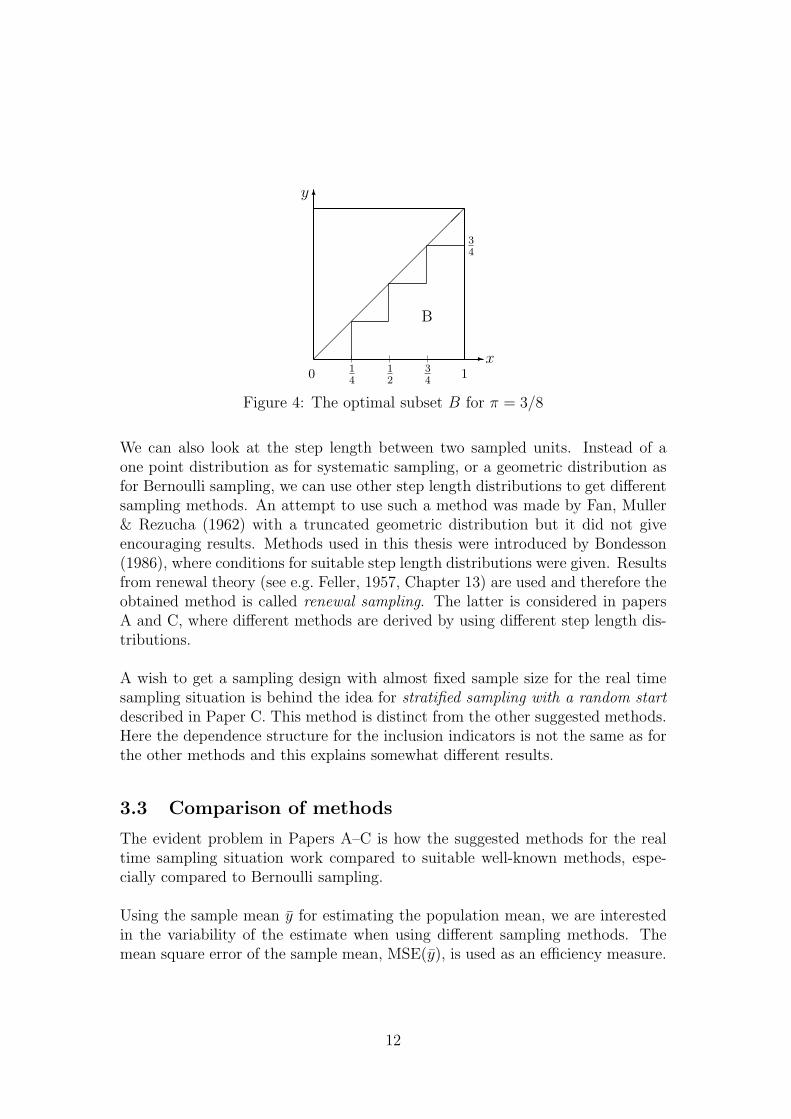
where h(·) is some function that gives negative correlations between the inclusionindicators. The choice of h(·) is a delicate task. We look at three cases – a linear,a product and a minimum function – where an explicit formula can be derivedfor the sampling correlations. An attempt to generalize this method by using ageometric approach is made. The focus is on the 2-dependent case, i.e. sets ofinclusion indicators more than lag 2 from each other are independent. We lookat a subset B of the unit cube and set Ii = 1 if (Ui−2, Ui−1, Ui) ∈ B. Here thequestion is how to choose B to get an efficient sampling method.

Figure 4 shows the form of a suitable B when using a unit square in the 1-dependent case.

11

-

6y

x0 1

412

34

1¡

¡¡

¡¡

¡¡

¡¡

¡¡¡

34

B

Figure 4: The optimal subset B for π = 3/8

We can also look at the step length between two sampled units. Instead of aone point distribution as for systematic sampling, or a geometric distribution asfor Bernoulli sampling, we can use other step length distributions to get differentsampling methods. An attempt to use such a method was made by Fan, Muller& Rezucha (1962) with a truncated geometric distribution but it did not giveencouraging results. Methods used in this thesis were introduced by Bondesson(1986), where conditions for suitable step length distributions were given. Resultsfrom renewal theory (see e.g. Feller, 1957, Chapter 13) are used and therefore theobtained method is called renewal sampling. The latter is considered in papersA and C, where different methods are derived by using different step length dis-tributions.

A wish to get a sampling design with almost fixed sample size for the real timesampling situation is behind the idea for stratified sampling with a random startdescribed in Paper C. This method is distinct from the other suggested methods.Here the dependence structure for the inclusion indicators is not the same as forthe other methods and this explains somewhat different results.

3.3 Comparison of methods

The evident problem in Papers A–C is how the suggested methods for the realtime sampling situation work compared to suitable well-known methods, espe-cially compared to Bernoulli sampling.

Using the sample mean y for estimating the population mean, we are interestedin the variability of the estimate when using different sampling methods. Themean square error of the sample mean, MSE(y), is used as an efficiency measure.

12

In Paper A, some of the methods are compared in a simulation study for a specialpopulation model. Here renewal sampling and sampling according to a stationaryprocess are studied among the new methods. Some good results are observed,but some final conclusions are that one should look at larger populations as wellas different population models.

For getting better insight when the new methods work well, some asymptoticcalculations are made in Paper B. We assume that the sequence of inclusion indi-cators, {Ii}, is a real stationary Bernoulli process in discrete time. Besides, someassumptions are made about the population structure. We look at the asymptoticmodel-based expectation of MSE(y) that depends on both model correlations andsampling correlations. We compare this quantity in the case of Bernoulli samplingand general sampling with negative sampling correlations. The question here isin which form the sampling correlations should be to gain most in efficiency byusing more advanced real time sampling methods.

Some restrictions are used for finding the best correlations. At first, we use thecondition 0 ≥ Rk ≥ −d, k = 1, 2, 3, . . ., where d is some constant depending onthe predetermined π-value. This condition is important for getting stable MSE-estimates. Also, a condition on the sum of sampling correlations is used; seebelow.

It appears that the sampling method with negative sampling correlations hasadvantages for a stationary population model with decreasing autocorrelations.The resulting optimal sampling correlations have a simple form. A samplingmethod with equal negative correlations R1 = R2 = . . . = Rm and Rk = 0for k > m, where m is some integer, has approximately an optimal structure.Therefore, to find sampling methods that allow such a correlation structure is ofgreat interest.

3.4 About stationary Bernoulli processes

In the following discussion the focus is mainly on m-dependent processes, i.e. setsof variables more than lag m apart are independent.

Let {Ii} be a stationary Bernoulli process in discrete time. Hence, we samplewith equal inclusion probabilities and the sampling correlations

Rk = Corr(Ii, Ii+k) =πi,i+k − π2

π(1− π)(3)

are equal for every two units k steps apart.

13

Since the proposed sampling methods are based on such Bernoulli processes asdescribed above, it is important to pay some attention to the properties of theseprocesses. Let m be some fixed integer. We want to sample units with a lag upto m apart dependently, and those more than lag m apart independently. Here,negative dependencies are desired and hence the sequences {Ii} such that Rk < 0for k = 1, 2, . . . , m, and 0 for k > m are of interest. The possible values of thesampling correlations play an important role. We would like to have these as neg-ative as possible for gaining most in efficiency compared to Bernoulli sampling.As seen from (3) there is an obvious lower bound for the correlation Rk, that isRk ≥ −π/(1 − π). However, more conditions are needed for getting a sequence{Ii} with desired properties.

A condition on the sum of sampling correlations is used due to the followingreasoning: Under which conditions is a sequence {Rk} with R0 = 1, Rk ≤ 0, k =1, 2, 3, . . . , a correlation sequence for a stationary Bernoulli process? In the cor-responding stationary normal process case with correlations r0 = 1, rk ≤ 0, k =1, 2, 3, . . ., the problem has a simple solution. In this case, it is shown in Bondes-son (2003) that a necessary and sufficient condition is

∞∑

k=1

rk ≥ −1

2.

In the Bernoulli case, the problem is more complicated. A necessary condition isthat the correlation sum is not lower than −1/2. This can be shown by lookingat the variance of the sum of the Bernoulli variables and using the fact that ithas to be nonnegative. The correlation sum

∑mk=1 Rk should preferably be close

to its lower bound. In Bondesson (2003), it is conjectured that for m = 1 thelower bound for the correlation sum is −1/3 at least for a 1-dependent sequenceand this still unproved conjecture is used in Paper B for finding the form of theoptimal correlations.

For m ≥ 2, however, the correlation sum can actually be below −1/3. There is nogeneral result about the lower limit in this case. To get better insight, correlationsums are studied for different sampling methods in Paper C. Numerical examplesabout possible negative correlations and minimum values of the correlation sumwith given values of π are presented for different sampling methods.

There are many different ways to derive sequences {Ii} with negative correla-tions. Many good results have been achieved but at the moment we can not givea simple general solution of how to define a sequence {Ii} with predeterminedπ, and with equal negative correlations R1 = R2 = . . . = Rm, and Rk = 0 fork > m. More research is certainly needed.

14

4 On distributional characteristics in sampling

The second half of the thesis includes three diverse papers about distributiontheory in survey sampling. As mentioned before, sampling design is a basic no-tion in sampling theory when using design-based and model-assisted approaches.In Section 2.1, a sampling design is defined as a probability distribution on sets.One can also consider the vector of inclusion indicators, I, here called a designvector, and define the multivariate distribution of I, p(k) = Pr(I = k), as asampling design, see e.g. Traat (2000). Here, k = (k1, k2, . . . , kN) is the outcomeof I and is an indicator of the realized sample, being always of dimension N .

This definition of a sampling design has some advantages. It covers both WR-and WOR-sampling designs and also uses the knowledge and tools worked outfor multivariate distributions (see e.g. Johnson, Kotz & Balakrishnan, 1997).The multivariate distribution of I is a multivariate Bernoulli distribution forWOR-sampling designs and some other multivariate discrete distribution for WR-sampling designs. Drawing a sample from a population U according to somesampling design means generating an outcome from a multivariate design distri-bution p(k).

The vector form of a sample can be naturally incorporated into the inferenceprocess. The design vector can be used in the definition of the survey data anddifferent statistics are functions of I and study variable values. This definition ofsampling design is used in Paper D for considering statistical inference in sam-pling. Here both the population model and the sampling design is included inthe inference, and characteristics of some estimators are considered.

A vector form of survey data makes it possible to use matrix tools in the samplingtheory. The way of expressing the sampling design as a multivariate distribution,as well as expressing the samples as vectors, is used by Ollila (2004), who con-siders different sample resampling methods for variance estimation.

Using the framework of the design vector, it is possible to give the probabilityfunction of a sampling design. Probability functions of several important sam-pling designs, e.g. the conditional Poisson, Sampford, and Pareto, are given inPaper E. Some different ways to use probability functions for drawing a sampleare described.

In Paper F, the main focus is on the π-estimator for the population total. We con-sider a design-based distribution of this estimator, and give design-based higher-order moments and cumulants which have not received so much attention in thesampling literature. Since the π-estimator is a linear function of the inclusion

15

indicators, its higher-order moments and cumulants depend on the respectivequantities of the inclusion indicators. Some attention is also paid to the varianceestimator of the π-estimator. It is well known that it is design-unbiased, but inthis paper its design-based variance is considered.

5 Summary of the papers

The present thesis contains six papers that consider different topics in surveysampling. In Papers A–C, we focus on the real time sampling situation andcorresponding sampling methods. Some sampling methods suitable for this caseare proposed and conditions giving efficient methods are considered. In Papers D–F, distribution theory in survey sampling is considered from different viewpoints.In Papers D and E, we use the design vector in the definition of the samplingdesign. In Paper D, unified inference is considered where both the populationmodel and the sampling design are taken into account. In Paper E, the focus is onprobability functions of different sampling designs. Formulae of the probabilityfunctions of several sampling designs are given. In Paper F, we consider thedesign-based distributional characteristics of the π-estimator of the populationtotal and its variance estimator.

Paper A. Some real time sampling methods

Let us consider a sampling situation where a finite population passes or is passedby the sampler. There is no list of the population and for every population unitthe sampler has to decide whether or not to sample a unit when he/she meets it.The population size N is most often unknown before the sampling but eventuallyit becomes known. Among the well-known methods, systematic sampling andPoisson (Bernoulli) sampling can be adopted for taking a sample in this samplingsituation. The aim of this paper is to find more suitable methods. We con-sider sampling methods with equal inclusion probabilities. Two general classesof sampling methods are introduced: renewal sampling and sampling accordingto a stationary process, which in some way take into account the pre-history ofthe sampling. To make some evaluation of these methods, a simulation studyis performed. Different methods with equal first-order inclusion probabilities arecompared numerically. In comparison with systematic sampling and Bernoullisampling, some promising results are derived for the new methods in the case ofa specific population model.

16

Paper B. Asymptotic considerations concerning real timesampling methods

A general real time sampling method with negative sampling correlations is con-sidered in this paper. This method is compared with Bernoulli sampling, havingindependent inclusion indicators and hence zero sampling correlations. The sam-pling correlations enter into the formulae of variances of different estimators andhence negative sampling correlations can contribute to reduced variances.

The aim of this paper is to find conditions under which the sampling methodwith negative sampling correlations should be used in favor of the well-knownBernoulli sampling. In other words: in which form should the correlations befor gaining most in efficiency using some more advanced sampling method thanBernoulli sampling? Some asymptotic calculations are made for finding the solu-tion to this problem. We assume some stationary model for the study variable.The asymptotic model-based expectation of the mean square error (MSE) of thesample mean is studied. It depends on both population model correlations andsampling correlations. Bernoulli sampling and general sampling with negativecorrelations are compared with respect to expected MSE, with some restrictionson the values of possible correlations.

It appears that the latter sampling method has advantages for a stationary pop-ulation model with decreasing autocorrelations. The optimal sampling correla-tions have a simple form and approximately optimal sampling designs should haveequal negative correlations for units up to lag m apart and zero correlations af-terwards. The achieved gain in efficiency depends also on how strongly correlatedthe population values are.

Paper C. Some different methods to get stationary Bernoullisequences with negative correlations for sampling applica-tions

In the previous paper we gave an approximately optimal form for sampling corre-lations to use to achieve more efficient sampling than standard Bernoulli sampling.The main question in this paper is how to get the nearly optimal sampling methodwith given first-order inclusion probabilities and negative sampling correlations.A stationary sequence of Bernoulli variables can be used as a tool for definingdifferent methods. Hence, problems such as how to get these Bernoulli sequencesand the correlation structure of these sequences are the main focus of this paper.Special attention is paid to the lowest possible correlation sum for given inclusionprobabilities and for different methods.

17

The emphasis is on finding a way to get a Bernoulli sequence with negative cor-relations and with as low correlation sum as possible. Special cases of samplingaccording to a stationary process and renewal sampling are studied. A generali-zation of Bernoulli sampling is obtained by using some function of independentuniform random variables for defining the Bernoulli variables. Further, a stratifi-cation method with random start is described. Numerical examples showing thelowest possible correlation sum for different methods are presented.

Paper D. Statistical inference in sampling theory

The framework with sampling design as a discrete multivariate distribution isused in this paper. This covers both with and without replacement samplingdesigns. We look at a unified approach where both the sampling design and thepopulation model are taken into account in inference. A general linear estimatorand its variance formula are given. It includes, for example, well-known design-based estimators as special cases. A two-phase sampling design is studied on amore general level where with and without replacement designs are allowed inboth phases.

Paper E. Sampling design and sample selection throughdistribution theory

We use a multivariate approach with a unifying treatment of with and withoutreplacement designs. The probability functions of several important sampling de-signs, such as hypergeometric, conditional Poisson, Sampford, and general ordersampling designs are presented. A list-sequential method for generating a samplefrom any given design using probability function is developed.

Paper F. The design-based distribution of some estimatorsin survey sampling

In this paper, we consider design-based distributional characteristics of the π-estimator for the population total. Usually only the design-based expected valueand variance are given in the sampling literature. General formulae for the design-based kth-order moments and cumulants of the π-estimator are presented in thispaper. The π-estimator is a linear function of the inclusion indicators, hence itskth-order moments and cumulants depend on the kth-order moments and cumu-lants of the inclusion indicators, respectively.

For estimating the variance of the π-estimator, an unbiased variance estimator isused. We give formulae for the design-based variance of this estimator and thecovariance of the π-estimator and its variance estimator.

18

6 Conclusions and open problems

The recent work of the author has concentrated on the real time sampling situa-tion. Hence, only questions arising in Papers A–C are treated in this section. Thetopics considered in the other papers have been developed further by others. Forexample, probability functions of some sampling designs are treated and appliedin Bondesson, Traat & Lundqvist (2004).

Consider real time sampling with equal inclusion probabilities. The initial goal ofthe work was to find suitable sampling methods (e.g. renewal sampling) and com-pare these to well-known methods that are possible to adopt in this case. Severalnew methods are proposed. All have in common that we in some way take intoaccount how the previous units are sampled and try not to sample units close toeach other so often, i.e. we sample with negative dependencies. It makes senseintuitively that in the real time sampling population, units close to each othermay have similar study variable values. Hence, the proposed methods shouldimprove the estimation.

We have chosen to study sampling methods with negative correlations mainlyin comparison to standard Bernoulli sampling, while using the sample mean asan estimator for the population mean. Also, we assume a stationary populationmodel with decreasing autocorrelations. In this case, we have found the formfor the nearly optimal sampling correlations by using asymptotic calculations.Here some restrictions on the sampling correlations are used. We gain most inefficiency using methods that give negatively correlated indicator variables andsuch that the correlation sum is small and that the correlations Rk are equal forunits up to lag m apart and zero afterwards.

Instead of giving further attention to the estimation problem, the focus haschanged to study sequences of negatively correlated Bernoulli variables. It isof main interest to study how to generate such sequences with desired properties.

As shown in Paper C, there are many different ways to get negative correlations.However, despite many attempts, a nice, simple, optimal solution for choosingwhich method to use for a given π-value to obtain the desired sampling corre-lations has not been found. Thus, practical suggestions for the sampler are notgiven. More research is certainly needed.

There is a difficult unsolved problem concerning the minimum value of the cor-relation sum. We have presented some numerical calculations of the correlationsum for different methods that give some possibility to compare these methodswith each other.

19

We do not assume that the population model is exactly true. Hence it is not al-ways clear what the best value of m should be. It depends both on conditions ofthe sampling correlations and also on the population model. For larger π-values,i.e. π close to 1/2, only units close to each other are usually sampled dependently.In the case of small π-values, we can have more correlations negative. It wouldbe of interest to study more how the estimates and variance estimates behave,depending on how many sampling correlations are negative. Here different popu-lation structures should give different results.

Would the form of the optimal sampling correlations hold also for other estima-tors? In the design-based framework, different estimators are functions of theinclusion indicators, hence sampling correlations enter into the variance formu-lae. If it is possible to have the variance estimator in Sen-Yates-Grundy form,then under some restrictions sampling with negative correlations should result inreduced variance.

Not much has been said about sampling with unequal inclusion probabilities.Sampling according to a stationary process can easily be extended to the case ofunequal probabilities. For the other methods it is not so obvious how to act forsampling with unequal probabilities. For instance, we can first apply samplingwith equal inclusion probabilities and then decide, for a selected unit, if it willbe sampled or not by using some predictions or auxiliary variables.

If the sampler determines the order of the units in the population (or the popu-lation units can order themselves), then Poisson sampling gives total protectionagainst subjective ordering bias. The methods proposed in this thesis protectpartially against such ordering. It would be of interest to find a measure of thisprotection.

The inclusion probability π is assumed to be determined before taking the sam-ple. However, the way of choosing the value of π has not been much discussed.Some guess about the population size N should be made.

The preliminary plans of this work also included a plan to use different methodson real data, for instance data from forestry. However, since the focus of the workchanged over time, this plan was set aside. Still, the author’s belief is that theideas behind the presented methods will eventually find good practical applica-tions.

20

References

Bondesson, L. (1986). Sampling of a linearly ordered population by selection ofunits at successive random distances. Report No. 25, Section of Forest Biometry,Swedish University of Agricultural Sciences, Umea.

Bondesson, L. (2003). On a Minimum Correlation Problem. Statistics & Proba-bility Letters, 62, 361–370.

Bondesson, L., Traat, I. and Lundqvist, A. (2004). Pareto Sampling versus Samp-ford and Conditional Poisson Sampling. Research Report 2004–6, Department ofMathematical Statistics, Umea University.

Feller, W. (1957). An Introduction to Probability Theory and Its Applications.Vol. I, 2nd ed. New York: Wiley.

Hansen, M. H., Dalenius, T. and Tepping, B. J. (1985). The development ofsample surveys of finite populations. In: A. C. Atkinson and S. E. Fienberg(eds.), A Celebration of Statistics: The ISI Centenary Volume, 327–354. NewYork: Springer–Verlag.

Hansen, M. H., Madow, W. G. and Tepping, B. G. (1983). An Evaluation ofModel-Dependent and Probability-Sampling Inference in Sample Surveys. Jour-nal of the American Statistical Association, 78, 776–793.

Horvitz, D. G. and Thompson, D. J. (1952). A generalization of sampling withoutreplacement from a finite universe. Journal of the American Statistical Associa-tion, 47, 663–685.

Husch, B., Miller, C. I. and Beers, T. W. (2003). Forest Mensuration. 4th ed.New York: Wiley.

Johnson, N. L., Kotz, S. and Balakrishnan, N. (1997). Discrete Multivariate Dis-tributions. New York: John Wiley.

Kalton, G. (2002). Models in the Practice of Survey Sampling (Revisited). Jour-nal of Official Statistics, 18, 129–154.

Little, R. J. (2004). To Model or Not To Model? Competing Modes of Inferencefor Finite Population Sampling. Journal of the American Statistical Association,99, 546–556.

Neyman, J. (1934). On the different aspects of the representative method: Themethod of stratified sampling and the method of purposive selection. Journal ofThe Royal Statistical Society, 97, 558–625.

Ollila, P. (2004). A Theoretical Overview for Variance Estimation in SamplingTheory with Some New Techniques for Complex Estimators. Research Report240, September 2004, Statistics Finland.

Raj, D. (1968). Sampling theory. New York: McGraw–Hill.

21

Rao, J. N. K. (1999). Some current trends in sample survey theory and methods.Sankhya, Ser. B, 61, 1–57.

Rao, J. N. K. and Bellhouse, D. R. (1990). History and Development of the The-oretical Foundations of Survey Based Estimation and Analysis. Survey Method-ology , 16, 3–29.

Royall, R. M. (1970). On finite population sampling theory under certain linearregression models. Biometrika, 57, 377–387.

Sarndal, C.–E. (1978). Design-based and Model-based Inference in Survey Sam-pling. Scandinavian Journal of Statistics, 5, 27–52.

Sarndal, C.–E., Swensson, B. and Wretman, J. (1992). Model Assisted SurveySampling. New York: Springer–Verlag.

Sen, A. R. (1953). On the estimate of the variance in sampling with varyingprobabilities. Journal of the Indian Society of Agricultural Statistics, 5, 119–127.

Traat, I. (2000). Sampling design as a multivariate distribution. In: T. Kollo,E.-M. Tiit and M. Srivastava, (eds), New trends in Probability and Statistics 5,Multivariate Statistics, 195–208. Vilnius, Utrecht: TEV/VSP.

Yates, F. and Grundy, P. M. (1953). Selection without replacement within stratawith probability proportional to size. Journal of the Royal Statistical Society,Ser. B, 15, 235–261.

22