on liapunov functional in theory of stability of systems with time-lag

Vol .9 N o . 4 A C T A M A T H E M A T I C A E A P P L I C A T A E S I N I C A Oc t . , 1993

ON LIAPUNOV FUNCTIONAL IN THEORY OF

STABILITY OF SYSTEMS WITH TIME-LAG't

W A N G LIAN (..~_ ~, :) WANG MUQIU ( . . ~ . . ~ . : ~ )

( In~itute ol Mathowatics, Acad~r,i~ $ini~, B~iji,~ 100080, Ch~'~)

A b s t r a c t

It is well known, that in the theory of stability in different.al equations, Liapunov's sec-

ond method may be the most important The center problem of Liapunov's second method is

construction of Liapunov function for concrete problems. Beyond any doubt, construct ion of Li-

apunov functions is an art. In the case of functional differential equations, there were also many

a t tempts to e~tablish various kinds of Liapunov type theorems. Recently Bur ton [2] presented an

excellent theorem using the Liapunov functional to solve the asymptotic stabili ty of functional

differential equation with bounded delay. However, the construction of such a Liapunov functional

is still very hard for concrete problems. In this paper, by utilizing this theorem due to Burton,

we construct concrete Liapunov functional forcer ta in and nonlinear delay differential equations

and derive new sufficient conditions for asymptotic stability. Those criteria improve the result of

l i terature [1] and they are with simple forms, easily checked and applicable.

§1. Introduction

With the development of modern science and technology, difference-differential equations (delay differential equation) have become an important and practical model for the control theorist, physicist, engineer, biologist and other scientists. For the theory of stability in differential equations, Liapunov's second method may be the most important. The central problem in Liapunov's second method is the construction of good Liapunov function for concrete problems. Beyond any doubt, the construction of Liapunov functions is an art. In the case of functional differential equations, there were also many attempts to establish various kinds of Liapunov type theorems. Recently, Burton [2] presented an excellent theorem using the Liapunov functional to solve the asymptotic stability of functional differential equation with bounded delay. However, the construction of such a Liapunov functional is still very hard for concrete problems. In this paper, by utilizing this theorem due to Burton, we construct concrete Liapunov functional for certain linear and nonlinear delay differential equations and derive new sufficient conditions for asymptotic stability. Our criteria improve the result in literature [1] and they are of simple forms, easily checked and applicable.

*Received Apr!l 3, 1990. Revised May 31, 1990.

tThis project is supported by the National Natural Science Foundation of China.

318 ACTA MATHEMATICAE APPLICATAE SINICA Vol.9

§2. Auxiliary Knowledge

Consider the system dx(t)

dt = F(t , zt) , (2.1}

where xt is a segment of x(s) on It - h, t] shifted to [ - h , 0I, h > 0 being a f ixed cons tan t . x E R n, Ixl = maXt<,<_n IxiI. For h > 0, C ( [ - h , 0] --* R n) denotes the space o f cont inuous funct ions m a p p i n g [ - h , 0] into R n, and for ~ E C, II~ll = sup_h<o<o I¢(0)l. c~, denotes the set of#b e O with I1¢11 < H. ~= b a continuous function of u defi~ed on -h < u < A, A > 0, and if t is a fixed number satisfying 0 < t < A, then xt denotes the restriction of x to the interval [t - h, t] so that xt is an element of C defined by xt(O} = x(t + 0) for --h < # < 0.

In {2.1), ~ denotes the right hand derivative of x at t and F(t, ~) E R" is continuous on [0, co) x OH.

We denote by x(to, ~) a solution of (2.1) with initial condition ~ E- CH where xto (to, ~o) = to and by x(t, to, ~) the value of x(to, ~o) at t.

It is supposed tha t F(t , O) = O, so tha t the zero function is a solution D e f i n i t i o n 2 .1 . If for each ~ > O, there exists a 6 = 6(,)>o. Such tha t

to>_0, t_>to and II~ll<a

imply Ix(t; to, ~o)I < e, then we say tha t the zero solution is uniformly stable. If, in addi t ion, there exists a 6 > 0 such tha t for any ~ > 0 there exists T = T ( t ) > 0, such t h a t

to >_ O, t >_ to + T, and 11~11<6

imply Ix(t; to, ~o)[ < e, then we say that x = 0 is uniformly asymptotically stable. Definition 2.2. Let V(t, ~o) be a scalar-valued continuous functional defined for t _> 0

and ~o E C([-h,0] ~ Rn). Then the derivative of V with respect to (2.1) is

dV(t,dt IP) (2.1) -- h--,o+lim h[VCt + h, xt+h(t, ~o)) -- V(t, !o)].

Moreover, if V(t, ¢(t}} e c t, then ~/ obtained by the chain rule, is

dr(t, ¢(t)) I = aV(t, ¢(t)) dt I(~.t) Ot

aV(t, ¢(t))F(t, ¢(t}). + 8x

Definition 2.3. The functional F(t, xt) win be called (a} continuous in t, if F(t, xt) is a continuous function of t for 0 _< t < +u whenever xt E CH, (b) locally Lipschitz with respect to xt if, for every ~ E [0, u) and every compact set L C CH, there exists a constant K~L > 0 such that

IF{t, xt) - F( t , Y,)I < KZLIIz - Ylll-h.tl

whenever t e [0, ~] and x,, y, e C([ -h , tl - . L). Theorem [2]. Let V(t, ~) and z(t, ~) : [0, oo) x CH ~ {0, co) be continuous and let

V(t, ~) be locally Lipschitz in ~o. Suppose that

z(t2, Io) - z ( t t , to) <. K( t2 - t l)

for some K > 0, with all ti and t2 satisfying 0 < tl < t2 < +oo, and all ~ E CH.

No.4 ON CONSTRUCTING LIAPUNOV FUNCTIONAL 319

and

If W(l~(o)l) + =(t, ~,) < v(t , ~,) <_ w,(l~(o)l) + ~(t, ~),

• (t , ~) _< W~(ll~ll)

dV(t, Xt) I } < -w~(l~(t)l),

d t (2.x) -

where w(l~l), W,(M), W2(ll~ll), W~(l~l) are all wedges, then the zero solution of (2.1) is uniformly asymptotically stable.

The proof of this theorem is omitted; see literature [2], p.252-254.

§3. G e n e r a l L i n e a r S y s t e m o f D i f f e r e n c e - d i f f e r e n t i a l E q u a t i o n s w i t h C o n s t a n t Coef f ic ien ts

Consider

dzi n n ~ " = E ai.izj(t) + ~ b'izi(t- 1"),

j = l 3"-----1

i = 1 , 2 , - - - , n , (3.1)

where a/j, bii, r > 0 ( i , j = 1, 2 , . . . ,n) axe all constants .

T h e o r e m $.1. If the coefficients ali, bii ( i , j = 1,2, .- . ,n) of system (3.1) satisfy the following conditions:

n

au+ In, l I+ ~ l b , , l < o, i = 2 i = 1

a23"4- ~ lai21+ ~ tbi21< O, i = 1 i = 1 i#2

t t--1

i = 1 i = 1

then the sero solution of (3.1) is asymptotically stable. P r o o [ . Define

n n / t t V(t, zd = ~ [z,(t)l + ~ K, Iz,(s)lds,

/ = 1 i = I - ~

where

(3.2)

x , = ~lb~, l . j=l

Definition 2.2 allows us to take a derivative of V(t, zt} with respect to (2.1), which is

dt

= d t S g x ~ ( t + O } + ~ K i ( l z i ( t ) [ - Iz~(t- r)[) ill i=1


= a~izj(t } + bijzi(t - "r) Sgn zi(t + O) + K~(Iz,(t)l- J=,(t - "r)l) / : 1 -- 3"=1 / : I

< ~ a.lxdt)[ + ~ la,;I lzi{t)l + ~ [bo'l Iz,'(t - r)l + K~(Iz,{t)J- Iz,(t - r}l) / : 1 j : l j : l

i : 1 j r 1

= , ,xx+ I ~ 1 + Ib.I l=xl+ " = + Y 2 ~ l ~ l + ~ - ~ l b , 2 1 1=21 i = 2 i : 1 i : 1 iffil

( ,), + ' " + ~ - , , + ~ l a , - I + bi~ z,~ I. i = 1 i = 1

It is evident that the upper and lower wedges are clear, that is,

n

W(l=l) =Wl(Ixl) = ~ I=,1, i = 1

,(t, ~) = Ib.,-,I I~,(.,)l e.., = w,(tl~ll}, i ~ l " : t - - T --3":1

W3(l=l) = - ~,~ + I,,,,,.I + ~ Ib,:',l I=.,.I + ~',--= + I",=1 + Ib,,~l Iz',l i : 2 / : I / : I / : i

,) ,] + . . . + a, , , ,+~-~lai , , l+ b,,, I z , , . /= l i = 1

Therefore the functional V(t, z,) and z(t, zt): 10, oo) x CH -'~ 10, oo) are continuous and V(t,~) is locally Lipschitz in ~. Moreover, owing to all Ibji[ (i,j = 1,2,-.-,n) being constants, the functional z(t, ~) has the following property:

z(t2, ~) - z(tx, ~) : Ibs, i Izi(s)[ ds - ~ Ibiil I=,(s)l d~ / : 1 : - r i : 1 t - r i : 1

j : l i : i

-. ,=1 ,=~ - Ib.,I I~ (-')1 I%

j = l x

for some K > O, with ail tl and t~ satisfying

O < t ~ < t2 < + o o and all ~oECH.


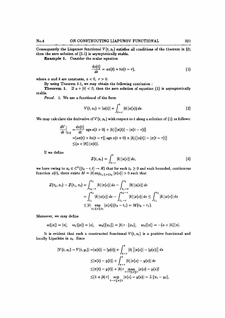
Consequently the Liapunov functional V(t, zt) satisfies all conditions of the theorem in §2; then the zero solution of (2.1} is asymptotically stable.

Example I. Consider the scalar equation

dz(t) = ,= ( t } + bx ( t - , ) , (X) dt

where a and b are constants, a < 0, r > 0. By using Theorem 3.1, we may obtain the following conclusion : Theorem I. If a + ]bl < 0, then the zero solution of equation {1} is asymptotically

stable. Proof. 1. We use a functional of the form

V(t, zt) = Ix(t)l + Ibl Iz(s)lds. {2)

We may calculate the derivative of V(t, xt) with respect to t Mong a solution of (I) as follows:

= lax ( t ) + ~x(t - , ) l sgn x( t + O) + i~i ( lx ( t ) l - ix( t - ~')1)

<-(,~+ Ibl ) Ix(t ) l .

If we def ine

ft t

z ( t , ~ d = . Ibl I~(~)ld,, (s) - - lr

we have owing to zt E C°([t0 -r,t] --* R) that for each to > 0 and each bounded, continuous function x(t), there exists M = Ibl'up,,<._<,: l~(s)l > 0 such that

z ( t~ , x,) - z ( tx , x~) = Ibl Ix(s)l ds - Ibl Ix(s)l ds

= Ibl I~(~)1 d., - Ibl I~(,)1 d~ _< Ibl I~(~)1 ds l ',#' t i - - ~ 1

< Ibi sup Ix(s) l ( t~ - t~) = M ( t ~ - t~). tl <s<tn

Moreover, we may define

~( Ix l ) = Ixl, ~x( Ix l ) = Ixl, ,,,=(llx, ll) - - I b l , . 11~,11, ~ ( I x l ) = - ( a + Ibl)lxl.

It is evident that such a constructed functional V(t, xt) is a positive functional and locally Lipschitz in zt. Since

IV(t, x,) -V( t , yt)l =Ix(t)]- ]y(t)l + Ibl [Iz(s)l- ly(s)l] ds

_<lx(tl - y(t) l + Ibl Ix(~) - ~(~)1 es m T

<Ix(t ) - y(t)l + Ibl ~ m ~ Ix(s) - y(~)l - t - , < s < _ t

<(l+lbll") sup Iz(s) -y(s) l=LI l xt--y,ll, t - r < s < t


where L --- 1 + [b I r > 0 is a constant, consequently the functional (2) satisfies all conditions of Burton's theorem in §2. Therefore, the zero solution of the equation (1} is asymptotically stable.

In literature [1], we have already used two methods to deal with the stability problem of {1}; one is the method of characteristic root, that is, to study the distribution of zero points of some elementary transcendental function. In practice such a research of the roots is difficult, and when the system considered is not autonomous or the time-lag variable of the system is a function of time t or not constant, all the results based on the %haxacteristic equation ~ are not applicable. Using of this method, we obtain the following conclusion for (1) (111, p.215-216).

Theorem 2. The zero solution of the equation (1) is asymptotically stable if and only if the coefficients a, b of (1) satisfy the inequahties:

(i) a + b < 0 , (ii}b 2 - a ~ < 0 . It explains that the condition a + Ibt < 0 given in Theorem 1 which guarantees the zero

solution of (1) is asymptotically stable is not only sufficient, but also necessary. It is also shown that the Liapunov functional (2) as given above is optimum with regard ~o (1}.

2. In the same way, we may use the other functional of the form

~t t (4)

where K is a positive constant to be specified below. We calculate the upper right derivative of V(t., xt},

dv(t,~, )

= 2 z ( t } ( a x ( t } + bx(t - r}) + K ( z 2 ( t } - 2=(t - r))

<(2a + g } x 2 ( t ) + Ibl ( ~ ( t ) + ~2(t - ~)) - g z 2 ( t - r};

when we choose K = ]bl, then we have

dV(t,dt x~) Ix~ - < 2(~ + Ibl)~2(t).

Consequently, if we let

~t t ~f

~(Ixt) = ~1(i~1) = ~2 w3(l~l) = - 2 ( ~ + 1@=2(t),

~,=(11~=,11) = Ibi~ sup ~ ( ~ ) = I b l . ~ i l ~ l l , t - r<s<t

then it is easy to see that the V ( t , xt) and Z(t , zt) are continuous and satisfy all conditions of B~rton's theorem in §2, therefore we obtain also the conclusion of Theorem 1. This also shows that the second Liapunov functional

~f t

v ( t , x , } = x2(t) + Iblx2(s)ds - - 1 "


is also optimum with regard to equation (1), hence Theorem 1 also improves the correspond- ing result in literature ([4] p. 252}, since the restriction on b > 0 given there is unnecessary.

E x a m p l e 2. Consider

dxl( t} dt = a , , ~ , ( t ) + ~ , , ~ ( t ) + b , , ~ ( t - , ) + b , : ~ : ( t - ~),

dz2(t) dt = , ,~lX,(t) + ~=x~( t ) + b~,~,( t - ,-) + b = ~ ( t - ,-),

(s)

where aq, biy, r > 0 ({,j ---- 1,2) are constants. For the same reason, we have the following conclusion.

T h e o r e m 8. If the coefficients of the system (5) satisfy the following two conditions:

(i) ql = a l l + la=l l + Ib,.,.I + Ib2,1 < o, (ii) q2 = a22 + lal21 + [hi21 + ]b22[ < O,

then the zero solution of system (5) is asymptotically stable. It is sufficient to take the functional of the form

~t t v(t ,~: , , y,) = (1~:~1 + I~1) + (K~I::~(*)I + K~l::~(s)l) d, , --T

where KI = Ibnl + ]b21l, K2 = lbl~l + Ib=l Although the conditions (i), (ii} are only sufficient, they are ve~ simple and easily

verified. 1. Consider

dx(t) _ -3z( t ) + by(t) + 2 z ( t - r) + 2Y(t - r), 1

dt dy(t) 1 1 1

dt = - ~ z ( t ) - 2y(t) + ~ x ( t - r) + ] y ( t - r), r > O . (6)

By Theorem 3, it is sufficient to choose the parameter b satisfying inequality ]b] < 45-, then the zero solution of system (6) is asymptotically stable.

2. Consider

dz(t) = -7z(t) + @y(t) + 4 z ( t - r) + by(t - r), 1

dt dy(t)

2z(t) - ay(t) + l x ( t - r) + 3y(t - r). dt

(7)

By Theorem 3, it is sufficient to choose the parameters a, b satisfying the following inequality

7 ~ + Ibl <

then the asymptotic stability of the zero solution of system (7) may be guaranteed.

§4. N o n l i n e a r S y s t e m w i t h C o n s t a n t T i m e - l a g

I. One dimensional nonlinear equation. Consider

d~(t) dt = - / ( ~ ( t ) ) + g(~( t - , ) ) , (4.1)

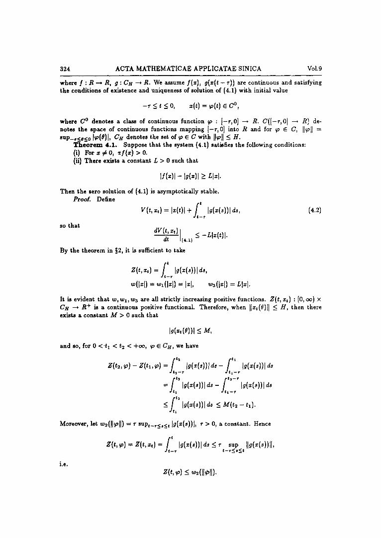
324 ACTA M A T H E M A T I C A E A P P L I C A T A E SINICA Vol.9

where I : R -+ R, g : C s --, R. We assume f ( z ) , g(z( t - , ) ) are continuous and satisfying the conditions of existence and uniqueness of solution of (4.1) with initial value

- , < t < 0, z(t) = ~o(t) E C °,

where U ° denotes a class of continuous function ~o : [ - r ,O} - - ~ R. C( [ - r ,O ] - - * R) denotes the space of continuous functions mapping [-r, 0] into R and for ~ E C, flail = sup_I,~8< 0 t~(e)l, C H denotes the set of ~ E C with II~II < H.

Theorem 4.1. Suppose that the system (4.1) satisfies the following conditions: (i} For = # O, ~ / ( z ) > 0. (ii) There exists a constant L > 0 such that

I f ( z ) l - lg(=)l-> LI=I.

Then the sero solution of (4.1) is ~ymptoticMly stable. Proof. Define

v ( t , , , ) - - I x ( t ) l + I g ( x ( s ) ) l ds, - - T

so that dV(t,.,)dt (4.1)

By the theorem in §2, it is sufficient to take

_< -L l= ( t ) l .

(4.2)

~ t z(t,x,) = Ig(=(8))l ds,

9(1=1) = 9~(1=1) = I=1, =3(1-1) =/1.1.

It is evident tha t w, wz, wa are all strictly increasing positive functions. Z(t, *t) : [0, oo) × CH ~ R + is a continuous positive functional. Therefore, when I(z=(O){l < jr./, then there exists a constant AI > 0 such that

Ig(z,(o))l < M, and so, for 0 < ' t I < t 2 < +oo, ~o E UH, we have

z(t~, ~) - z(t,, ~) ~t t2 ~t tl = Ig(.=.(s))l d,, - 2 --/" I --T =fi'

-< ~'t,,, 1

Ig(*C~))ld~

Ig(=(s))l ds _ M( ,2 - t , ) .

Moreover, let 92(11~011 ) = T sup,_,<,<¢ Ig(z(s))I, r > O, a constant. Hence

~ t z(,,~) = z(,,.=) = Ig(=(s))Id~ ~ ~ sup llg(~(~))ll, - r t - r < 8 _ ~ t

i.e. z(,, ~) _< 92(li~fl).


Consequently, the Liapunov function V(t, xt) given by us for equation (4.2) satisfies all conditions of the theorem in §2, and the zero solution of (4.1) is asymptotically stable.

Example 1. Consider

dz(t) = -(2=(t)+ =3@ + ~=3(t- ~), (A) dt

where f(x} = 2z + z3 g(x} = ½z3. Owing to

I f ( = ) l - 19(=)1 >- 21=1, and z # 0, =f(=) > 0,

consequently, by Theorem 4.1, know that the zero solution of equation (A) is asymptotically stable.

II. Two dimensional non-linear system Consider

dz(t) dt = - f 1 ( z ) + aly + g l ( z ( t - r ) ) + b l y ( t - v), (4.3)

dy(t ) = a2x - [2(Y} + b2x(t - r) + g2(y(t - r)), dt

where we assume that f l (=) , f2(Y} a r e continuous, and h(0) = f2(0) = 0, gi : C H { ( x t , y t ) T : I1=,11 -< H, IIv, II -< H } -~ R = (~ = 1,2), are continuous and g,(0) = g=(O) = 0.

C{(z, y}r: [--r, O] ---* R 2} denotes the class of continuous vector function (z(t), y(t))T : I - r , 0] --* R ~. In addition, we suppose still that the right hand of (4.3) satisfies some conditions which guarantee the existence and uniqueness of solution of (4.3) with the following initial value

=(t) = ~(t) , y( t )~ ¢(t) for - ~ < t < 0.

T h e o r e m 4.2. If the system (4.3) satisfies the following conditions: (i} When = # O, x l x (= } > 0; y # O, y f2(y ) > O. (ii} There exist two constants al > 0, a2 > 0 such that

I / , ( = ) 1 - [ Ig,(=)l + (la21 + Ib21)I=1] --- ~, I=1, lY=(v)I- [Ig=(v)l + (I,,I + Ih l ) ly l ] -> ~=lyl,

then the zero solution of system (4.3) is asymptotically stable. Proof. In order to study the stability of the zero solution, we make use of a Liapunov

functional of the form

v(y,=,,v,) = I=1 + Ig~(=(s})lds + Ib=l Iz(s)lds -" -" (4.4) [ f ' f' ] + Ivl + Ig=(v(,))l d, + Ib,I Iv(s)l ds .

- - I " - - T

Regaxding the derivative of V(t, xt,yt) along solutions of (4.3) with respect to t, we may calculate

~ ( t , =,, v,) dt (4.3}

=d_~x sgnz(t + 0} + Ig , ( z ( t ) ) l - I # , (= ( t - r)) l + Ib21 (I=(t)l - Ix( t - ~)[) dt

dy sgn v(t + 0) + Ig= (y ( t ) ) l - Ig= (v ( t - " ) )1+ Ib, I ( M t ) l - Iv(t - ,)1) + - ~

-< - [ I h ( = ) l - 19 , (=)1- Ib=l I =1 - I~=1 I=1] - [ l f = ( v ) l - Ig=(Y) l - Ib, I I v l - I~,11vl]

-< - (~1=1 + ~=lvl).


Here, we should point out that it is sufficient to take

~1(=, y) =~o(=, y) = I=1 + lYl, w3(=, y} =,~x I'~1 + ~ lyl,

// f/ z(t,z,,y,) = lg,(z(s))l ds + Ib=l I~(~)lds --,#. __f .

f/ f,' + I~(y(s))l as + Ibxl ly(s)l ds;

then we know that the functional V(t, zt,yt) given by (4.4) satisfies all conditions of the theorem in §2. Consequently the zero solution of (4.3} is asymptotically stable.

Example I. Consider

dy(t) = _4~(t)_1 _ 4y(t) - 3y3(t) + ~( t - , ) _ _15y3( t _ ,). dt

(4.5)

In fact, it is sufficient to take the functional of the form

I f , f,' ] * l l~3(d lds + I~:(dl a~ v ( t , . , , y,) = I*1 + - , ~ - ,

+ [lY'+ f'_,. ~ly3{s)lds + ft. luO)l as], (4.6)

so that dV (t, xt, yt) p l

5 _< - 4 1 z ( t ) l - dt ¢4.s) 2 ly(t)l"

By Theorem 4.2, it follows that the zero solution of (4.5) is asymptotically stable. III. n-dimensional nonlinear system In the same way, we may consider

dx,(t) " dt = - f{(zi(t)) + gi(z i ( t - r)) + Z aqzj(t) + b i j z i ( t - f),

j= , . j# i i=I j '# i (4.7)

i = 1 , 2 , - . . , n .

Here, still as above, we assume that the right hand of system (4.7) is defined on the product space

CH X R" -~ R ~,

and they are continuous and satisfy some conditions which guarantee the existence and uniqueness of solution of (4.7) with initial value

z~ ( t }=~ , ( t ) for - r < t _ < O , i = 1 , 2 , . - - , n ,

in addition, I , ( 0 ) = 0 , g~(0)=0, i = 1 , 2 , ,n,

r > 0 being an arbitrary constant. We have the following conclusion: T h e o r e m 4.3. If the system (4.7) satisfies the following conditions:

No .4 ON CONSTRUCTING LIAPUNOV FUNCTIONAL 327

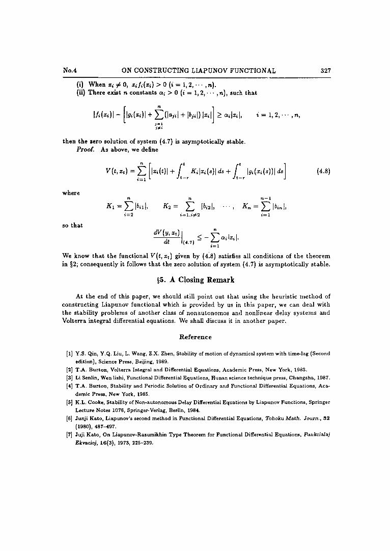
(i} When z, ~ O, z i f i ( z i ) > 0 (i = 1,2, . . . ,n). (ii) There exist n constants ai > 0 (i = 1, 2 , . . . , n), such that

[ n ] I ! , ( ~ , ) l - Ig,(z,)l + ~ ( 1 ~ , , 1 + Ibj, I)Ix, I > ~,lx, I,

then the zero solution of system (4.7) is asymptotically stable. Proo£. As above, we define

i = 1 , 2 , - . - , n ,

/' f' ] v(t, =,) = I~,(t)l + K, l~ (s ) l d8 + 19,(~,(s))l d~ i = 1 - r --~

(4.8)

where

so that

g l = Ibitl, K2 = Ib,~l, " . . , g,~ = E I b''*l' i = 2 i = 1 , i ; ~ 2 i = 1

dV(Y' zd 1 ( 4 . r ) d t - < - ~ a~lz~J. i=1

We know that the functional V(t , xt) given by (418) satisfies all conditions of the theorem in §2; consequently it follows that the zero solution of system (4.7} is asymptotically stable.

§5. A C los ing R e m a r k

At the end of this paper, we should still point out that using the heuristic method of constructing Liapunov functional which is provided by us in this paper, we can deal with the stability problems of another class of nonautonomos and nonlinear delay systems and Volterra integral differential equations. We shall discuss it in another p~per.

Reference

[1] Y.S. Qin, Y.Q. Liu, L. Wang, Z.X. Zhen, Stability of motion of dynamical system with time-lag (Second edition), Science Press, Beijing, 1989.

[2] T.A. Burton, Volterra Integral and Differential Equations, Academic Press, New York, 1983. [3] Li Senlin, Wen lizhi, Functional Differential Equations, Hunan science technique press, Changsha, 1987. [4] T.A. Burton, Stability and Periodic Solution of Ordinary and Functional Differential Equations, Aca-

demic Press, New York, 1985. [5] K.L. Cooke, Stability of Non-autonomous Delay Differential Equations by Liapunov Functions, Springer

Lecture Notes 1076, Springer-Verlag, Berlin, 1984.

[6] Junji Kato, Liapunov's second method in Functional Differential Equations, Tohoku Math. Journ., 32

(1980), 487--497. [7] Juji Kato, On Liapunov-Rasumikhin Type Theorem for Functional Differential Equations, Funkcia/aj

Ekv~cioj, 16(3), 1973, 225-239.

on liapunov functional in theory of stability of systems with time-lag

Documents