on kronecker products, tensor products and matrix ... · tensor products and matrix derivatives...

On Kronecker Products, Tensor Products and Matrix Differential Calculus

Stephen Pollock, University of Leicester, UK

Working Paper No. 14/02

February 2014

ON KRONECKER PRODUCTS, TENSOR PRODUCTSAND MATRIX DIFFERENTIAL CALCULUS

By D.S.G. Pollock

University of Leicester

Email: stephen [email protected]

The algebra of the Kronecker products of matrices is recapitulated using a

notation that reveals the tensor structures of the matrices. It is claimed that

many of the difficulties that are encountered in working with the algebra

can be alleviated by paying close attention to the indices that are concealed

beneath the conventional matrix notation.

The vectorisation operations and the commutation transformations

that are common in multivariate statistical analysis alter the positional

relationship of the matrix elements. These elements correspond to numbers

that are liable to be stored in contiguous memory cells of a computer, which

should remain undisturbed.

It is suggested that, in the absence of an adequate index notation that

enables the manipulations to be performed without disturbing the data,

even the most clear-headed of computer programmers is liable to perform

wholly unnecessary and time-wasting operations that shift data between

memory cells.

1. Introduction

One of the bugbears of multivariate statistical analysis is the need to differen-tiate complicated likelihood functions in respect of their matrix arguments. Toachieve this, one must resort to the theory of matrix differential calculus, whichentails the use of Kronecker products, vectorisation operators and commutationmatrices.

A brief account of the requisite results was provided by Pollock (1979),who described a theory that employs vectorised matrices. Relationships wereestablished with the classical theory of Dwyer and McPhail (1948) and Dwyer(1967), which dealt with scalar functions of matrix augments and matrix func-tions of scalar arguments. A contemporaneous account was given by Hendersonand Searle (1979), and similar treatments were provided, at roughly the sametime, by Balestra (1976) and by Rogers (1980).

A more extensive account of matrix differential calculus, which relies ex-clusively on vectorised matrices, was provided by the text of Magnus andNeudecker (1988). This has become a standard reference. More recent ac-counts of matrix differential calculus have been provided by Turkington (2002)and by Harville (2008).

Notwithstanding this ample provision of sources, there continues to beconfusion and difficulty in this area. A recent paper of Magnus (2010), which

1

D.S.G. POLLOCK

testifies to these problems, cites several instances in which inappropriate def-initions of matrix derivatives have been adopted, and it gives examples thathighlight the perverse effects of adopting such definitions.

One is bound to wonder why the difficulties persist. An answer to thisconundrum, which is offered in the present paper, points to the absence ofan accessible account that reveals the tensorial structures that underlie theessential results of matrix differential calculus and of the associated algebra.

Part of the problem lies in the fact that the conventional matrix notation,which has been employed, almost exclusively, to convey the theory of matrixdifferential calculus, conceals the very things that need to be manipulated,which are matrix elements bearing strings of indices that are ordered accordingto some permutation of a lexicographic ordering. To overcome the problem, weshall adopt a notation that reveals the indices.

This paper aims to avoid unnecessary abstractions by dealing only withconcrete objects, which are matrices and their elements. A more abstract ap-proach would employ the concepts and the notations of vector spaces and oftheir tensor products. Such an approach to the theory is exemplified by thetexts in multilinear algebra of Bourbaki (1958), Greub (1967) and Marcus(1973). A primary source of multilinear algebra and differential geometry isCartan (1952). One advantage of the approach that we shall take is that it iswell adapted to the requirements of computer programming.

2. Bases for Vector Spaces

Consider an identity matrix of order N , which can be written as follows:

(1) [ e1 e2 · · · eN ] =

1 0 · · · 00 1 · · · 0...

.... . .

...0 0 · · · 1

=

e1

e2

...eN

.

On the LHS, the matrix is expressed as a collection of column vectors, denotedby ei; i = 1, 2, . . . , N , which form the basis of an ordinary N -dimensional Eu-clidean space, which is the primal space. On the RHS, the matrix is expressedas a collection of row vectors ej ; j = 1, 2, . . . , N , which form the basis of theconjugate dual space. In general, vetors bearing a single superscript, includinga prime, are to be regarded as row vectors.

The basis vectors can be used in specifying arbitrary vectors in both spaces.In the primal space, there is the column vector

(2) a =X

i

aiei = (aiei),

and in the dual space, there is the row vector

(3) b0 =X

j

bjej = (bje

j).

2

TENSOR PRODUCTS and MATRIX DERIVATIVES

Here, on the RHS, there is a notation that replaces the summation signs byparentheses. When a basis vector is enclosed by parentheses, summations areto be taken in respect of the index or indices that it carries. Usually, suchindices will be associated with scalar elements that will also be found withinthe parentheses. The advantage of this notation will become apparent at alater stage, when the summations are over several indices.

A vector in the primary space can be converted to a vector in the conjugatedual space, and vice versa, by the operation of transposition. Thus, a0 = (aiei)is formed from a = (aiei) via the conversion ei → ei, whereas b = (bjej) isformed from b0 = (bjej) via the conversion ej → ej .

3. Elementary Tensor Products

A tensor product of two vectors is an outer product that entails the pairwiseproducts of the elements of both vectors. Consider two primal vectors

(4)a = [at; t = 1, . . . T ] = [a1, a2, . . . , bT ]0 andb = [bj ; j = 1, . . . ,M ] = [b1, b2, . . . , bM ]0,

which need not be of the same order. Then, two kinds of tensor products canbe defined. First, there are covariant tensor products. The covariant productof a and b is a column vector in a primal space:

(5) a⊗ b =X

t

X

j

atbj(et ⊗ ej) = (atbjetj).

Here, the elements are arrayed in a long column in an order that is determinedby the lexicographic variation of the indices t and j. Thus, the index j under-goes a complete cycle from j = 1 to j = M with each increment of the index tin the manner that is familiar from dictionary classifications. Thus

(6) a⊗ b =

a1ba2b...

aT b

= [a1b1, . . . , a1bM , a2b1, . . . , a2bM , · · · , aT b1, . . . , aT bM ]0.

A covariant tensor product can also be formed from the row vectors a0 andb0 of the dual space. Thus, there is

(7) a0 ⊗ b0 =X

t

X

j

atbj(et ⊗ ej) = (atbjetj).

It will be observed that this is just the transpose of a⊗ b. That is to say,

(8) (a⊗ b)0 = a0 ⊗ b0 or, equivalently, (atbjetj)0 = (atbjetj).

3

D.S.G. POLLOCK

The order of the vectors in a covariant tensor product is crucial, since, asone can easily verify, it is the case that

(9) a⊗ b 6= b⊗ a and a0 ⊗ b0 6= b0 ⊗ a0.

The second kind of tensor product of the two vectors is a so-called con-travariant tensor product:

(10) a⊗ b0 = b0 ⊗ a =X

t

X

j

atbj(et ⊗ ej) = (atbjejt ).

This is just the familiar matrix product ab0, which can be written variously as

(11)

a1b0

a2b0...

aT b0

= [ b1a b2a · · · bMa ] =

a1b1 a1b2 . . . a1bM

a2b1 a2b2 . . . a2bM...

......

aT b1 aT b2 . . . aT bM

.

According to (10), the ordering of the vectors within such a binary contravarianttensor product is immaterial, albeit that ab0 6= b0a.

Observe that

(12) (a⊗ b0)0 = a0 ⊗ b or, equivalently, (atbjejt )0 = (atbje

tj).

We now propose to dispense with the summation signs and to write thevarious vectors as follows:

(13) a = (atet), a0 = (atet) and b = (ajej), b0 = (bje

j).

As before, the convention here is that, when the products are surrounded byparentheses, summations are to be taken in respect of the indices that areassociated with the basis vectors.

The convention can be applied to provide summary representations of theproducts under (5), (7) and (10):

a⊗ b = (atet)⊗ (bjej) = (atbjetj),(14)

a0 ⊗ b0 = (atet)⊗ (bje

j) = (atbjetj),(15)

a⊗ b0 = (atet)⊗ (bjej) = (atbje

jt ).(16)

Such products are described as decomposable tensors.

4. Non-decomposable Tensor Products

Non-decomposable tensors are the result of taking weighted sums of decompos-able tensors. Consider an arbitrary matrix X = [xtj ] of order T ×M . This can

4


be expressed as the following weighted sum of the contravariant tensor productsformed from the basis vectors:

(17) X = (xtjejt ) =

X

t

X

j

xtj(et ⊗ ej).

The indecomposability lies in the fact that the elements xtj cannot be writtenas the products of an element indexed by t and an element indexed by j.

From X = (xtjejt ), the following associated tensors products may be de-

rived:

X 0 = (xtjetj),(18)

Xr = (xtjetj),(19)

Xc = (xtjejt).(20)

Here, X 0 is the transposed matrix, whereas Xc is a long column vector and Xr

is a long row vector. Notice that, in forming Xc and Xr from X, the indexthat moves assumes a position at the head of the string of indices to which it isjoined. It will be observed that whereas the indices of the elements of Xr followa lexicographic ordering, with the leading index as the principal classifier, thoseof Xc follow a reverse lexicographic ordering.

The superscript letters c and r denote a pair of so-called vectorisationoperators. It has become conventional to denote Xc by vecX. Turkington(2000 and 2002) has used the notation devecX = (vecX 0)0 to denote Xr andto indicate its relationship with vecX.

It is evident that

(21) Xr = X 0c0 and Xc = X 0r0.

Thus, it can be seen that Xc and Xr are not related to each other by simpletranspositions.

The transformation that effects the reversal of the ordering of the twoindices, and which thereby reverses the order of the vectors in a covarianttensor product, was described by Pollock (1979) as the tensor commutator.The transformation was denoted by a capital T inscribed in a circle. Thecopyright symbol is also an appropriate choice of notation, which leads one towrite

(22) Xr0 = X 0c = c©Xc and Xc = c©X 0c.

It will be shown in Section 7 that the transformation c© corresponds to anorthonormal matrix. This was described by Magnus and Neudecker (1979) asthe commutation matrix, which they denoted by K.

Example. Consider the equation

(23) ytj = µ + γt + δj + εtj

5

D.S.G. POLLOCK

wherein t = 1, . . . , T and j = 1, . . . ,M . This relates to a two-way analysis ofvariance. For a concrete interpretation, we may imagine that ytj is an obser-vation taken at time t in the jth region. Then, the parameter γt represents aneffect that is common to all observations taken at time t, whereas the parameterδj represents a characteristic of the jth region that prevails through time.

In ordinary matrix notation, the set of TM equations becomes

(24) Y = µιT ι0M + γι0M + ιT δ0 + E ,

where Y = [ytj ] and E = [εtj ] are matrices of order T ×M , γ = [γ1, . . . , γT ]0and δ = [δ1, . . . , δM ]0 are vectors of orders T and M respectively, and ιT andιM are vectors of units whose orders are indicated by their subscripts. In termsof the index notation, the TM equations are represented by

(25) (ytjejt ) = µ(ej

t ) + (γtejt ) + (δje

jt ) + (εtje

jt ).

An illustration is provided by the case where T = M = 3. Then equations(24) and (25) represent the following structure:

(26)

y11 y12 y13

y21 y22 y23

y31 y32 y33

= µ

1 1 11 1 11 1 1

+

γ1 γ1 γ1

γ2 γ2 γ2

γ3 γ3 γ3

+

δ1 δ2 δ3

δ1 δ2 δ3

δ1 δ2 δ3

+

ε11 ε12 ε13

ε21 ε22 ε23

ε31 ε32 ε33

.

5. Multiple Tensor Products

The tensor product entails an associative operation that combines matrices orvectors of any order. Let B = [blj ] and A = [aki] be arbitrary matrices oforders t× n and s×m respectively. Then, their tensor product B ⊗A, whichis also know as a Kronecker product, is defined in terms of the index notationby writing

(27) (bljejl )⊗ (akie

ik) = (bljakie

jilk).

Here, ejilk stands for a matrix of order st×mn with a unit in the row indexed

by lk—the {(l − 1)s + k}th row—and in the column indexed by ji—the {(j −1)m + i}th column—and with zeros elsewhere.

In the matrix array, the row indices lk follow a lexicographic order, asdo the column indices ji. Also, the indices lk are not ordered relative to theindices ji. That is to say,

(28)

ejilk = el ⊗ ek ⊗ ej ⊗ ei

= ej ⊗ ei ⊗ el ⊗ ek

= ej ⊗ el ⊗ ek ⊗ ei

= el ⊗ ej ⊗ ei ⊗ ek

= el ⊗ ej ⊗ ek ⊗ ei

= ej ⊗ el ⊗ ei ⊗ ek.

6


The virtue of the index notation is that it makes no distinction amongst thesevarious products on the RHS—unless a distinction can be found between suchexpressions as ej i

l k and e j il k .

For an example, consider the Kronecker of two matrices as follows:

(29)

∑b11 b12

b21 b22

∏⊗

∑a11 a12

a21 a22

∏=

b11

∑a11 a12

a21 a22

∏b12

∑a11 a12

a21 a22

∏

b21

∑a11 a12

a21 a22

∏b22

∑a11 a12

a21 a22

∏

=

b11a11 b11a12

b11a21 b11a22

b12a11 b12a12

b12a21 b12a22

b21a11 b21a12

b21a21 b21a22

b22a11 b22a12

b22a21 b22a22

.

Here, it can be see that the composite row indices lk, associated with theelements bljaki, follow the lexicographic sequence {11, 12, 21, 22}. The columnindices follow the same sequence.

6. Compositions

In order to demonstrate the rules of matrix composition, let us consider thematrix equation

(30) Y = AXB0,

which can be construed as a mapping from X to Y . In the index notation, thisis written as

(31)(ykle

lk) = (akie

ik)(xije

ji )(blje

lj)

= ({akixijblj}elk).

Here, there is

(32) {akixijblj} =X

i

X

j

akixijblj ;

which is to say that the braces surrounding the expression on the LHS are toindicate that summations are taken with respect to the repeated indices i andj, which are associated with the basis vectors. The operation of composingtwo factors depends upon the cancellation of a superscript (column) index, orstring of indices, in the leading factor with an equivalent subscript (row) index,or string of indices, in the following factor.

The matrix equation of (30) can be vectorised in a variety of ways. Inorder to represent the mapping from Xc = (xijeji) to Y c = (yklelk), we maywrite

(33)(yklelk) = ({akixijblj}elk)

= (akibljejilk)(xijeji).

7

D.S.G. POLLOCK

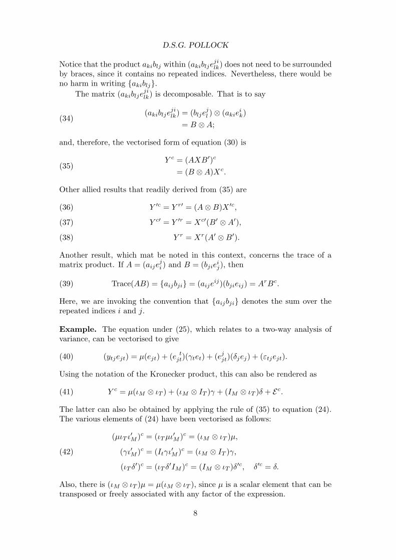
Notice that the product akiblj within (akibljejilk) does not need to be surrounded

by braces, since it contains no repeated indices. Nevertheless, there would beno harm in writing {akiblj}.

The matrix (akibljejilk) is decomposable. That is to say

(34)(akiblje

jilk) = (blje

jl )⊗ (akie

ik)

= B ⊗A;

and, therefore, the vectorised form of equation (30) is

(35)Y c = (AXB0)c

= (B ⊗A)Xc.

Other allied results that readily derived from (35) are

Y 0c = Y r0 = (A⊗B)X 0c,(36)

Y c0 = Y 0r = Xc0(B0 ⊗A0),(37)

Y r = Xr(A0 ⊗B0).(38)

Another result, which mat be noted in this context, concerns the trace of amatrix product. If A = (aije

ji ) and B = (bjiei

j), then

(39) Trace(AB) = {aijbji} = (aijeij)(bjieij) = ArBc.

Here, we are invoking the convention that {aijbji} denotes the sum over therepeated indices i and j.

Example. The equation under (25), which relates to a two-way analysis ofvariance, can be vectorised to give

(40) (ytjejt) = µ(ejt) + (e tjt)(γtet) + (ej

jt)(δjej) + (εtjejt).

Using the notation of the Kronecker product, this can also be rendered as

(41) Y c = µ(ιM ⊗ ιT ) + (ιM ⊗ IT )γ + (IM ⊗ ιT )δ + Ec.

The latter can also be obtained by applying the rule of (35) to equation (24).The various elements of (24) have been vectorised as follows:

(42)

(µιT ι0M )c = (ιT µι0M )c = (ιM ⊗ ιT )µ,

(γι0M )c = (Itγι0M )c = (ιM ⊗ IT )γ,

(ιT δ0)c = (ιT δ0IM )c = (IM ⊗ ιT )δ0c, δ0c = δ.

Also, there is (ιM ⊗ ιT )µ = µ(ιM ⊗ ιT ), since µ is a scalar element that can betransposed or freely associated with any factor of the expression.

8


In comparing (40) and (41), we see, for example, that (e tjt) = (ej)⊗ (et

t) =ιM ⊗ IT . We recognise that (et

t) is the sum over the index t of the matricesof order T which have a unit in the tth diagonal position and zeros elsewhere;and this sum amounts, of course, to the identity matrix of order T .

The vectorised form of equation (26) is

(43)

y11

y21

y31

y12

y22

y32

y13

y23

y33

=

1 1 0 0 1 0 01 0 1 0 1 0 01 0 0 1 1 0 0

1 1 0 0 0 1 01 0 1 0 0 1 01 0 0 1 0 1 0

1 1 0 0 0 0 11 0 1 0 0 0 11 0 0 1 0 0 1

µ

γ1

γ2

γ3

δ1

δ2

δ3

+

ε11

ε21

ε31

ε12

ε22

ε32

ε13

ε23

ε33

.

7. The Commutation Matrix

The transformation X 0c = c©Xc from Xc = (xtjejt) to X 0c = (xtjetj) is effectedby the commutation matrix c© = (ejt

tj). Thus

(44) (xtjetj) = (ejttj)(xtjejt).

It is easy to see that c© is an orthonormal matrix with c©0 = c©−1.Any pair of covariant indices that are found within a multiple tensor prod-

uct may be commuted. Thus, for example, there is

(45) c©(A⊗B) c© = (B ⊗A),

which is expressed in the index notation by writing

(46) (ekllk)({akiblj}eij

kl)(ejiij) = ({bljaki}eji

lk).

Here, the four indices may have differing ranges and, therefore, the two com-mutation matrices of equation (45) may have differing structures and orders.Nevertheless, we have not bothered to make any notational distinction betweenthem. If such a distinction were required, then it might be achieved by attach-ing to the symbols the indices that are subject to commutations.

Observe also that the braces, which have been applied to the scalar product{akiblj} in equation (46), are redundant, since the string contains no repeatedindices. Their only effect it to enhance the legibility.

Matrices that perform multiple commutations have been defined by Abadirand Magnus (2005) and by Turkington (2002). Such matrices can be composed

9

D.S.G. POLLOCK

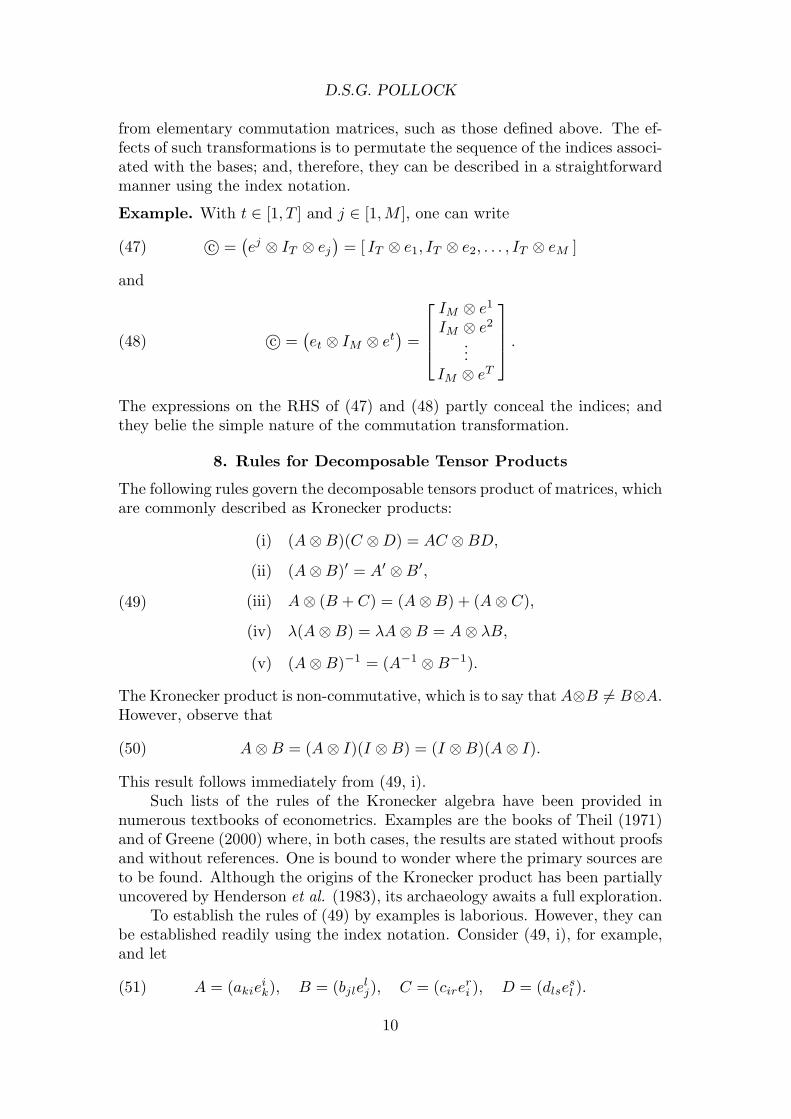
from elementary commutation matrices, such as those defined above. The ef-fects of such transformations is to permutate the sequence of the indices associ-ated with the bases; and, therefore, they can be described in a straightforwardmanner using the index notation.

Example. With t ∈ [1, T ] and j ∈ [1,M ], one can write

(47) c© =°ej ⊗ IT ⊗ ej

¢= [ IT ⊗ e1, IT ⊗ e2, . . . , IT ⊗ eM ]

and

(48) c© =°et ⊗ IM ⊗ et

¢=

IM ⊗ e1

IM ⊗ e2

...IM ⊗ eT

.

The expressions on the RHS of (47) and (48) partly conceal the indices; andthey belie the simple nature of the commutation transformation.

8. Rules for Decomposable Tensor Products

The following rules govern the decomposable tensors product of matrices, whichare commonly described as Kronecker products:

(49)

(i) (A⊗B)(C ⊗D) = AC ⊗BD,

(ii) (A⊗B)0 = A0 ⊗B0,

(iii) A⊗ (B + C) = (A⊗B) + (A⊗ C),

(iv) λ(A⊗B) = λA⊗B = A⊗ λB,

(v) (A⊗B)−1 = (A−1 ⊗B−1).

The Kronecker product is non-commutative, which is to say that A⊗B 6= B⊗A.However, observe that

(50) A⊗B = (A⊗ I)(I ⊗B) = (I ⊗B)(A⊗ I).

This result follows immediately from (49, i).Such lists of the rules of the Kronecker algebra have been provided in

numerous textbooks of econometrics. Examples are the books of Theil (1971)and of Greene (2000) where, in both cases, the results are stated without proofsand without references. One is bound to wonder where the primary sources areto be found. Although the origins of the Kronecker product has been partiallyuncovered by Henderson et al. (1983), its archaeology awaits a full exploration.

To establish the rules of (49) by examples is laborious. However, they canbe established readily using the index notation. Consider (49, i), for example,and let

(51) A = (akieik), B = (bjle

lj), C = (cire

ri ), D = (dlse

sl ).

10


Then,

(52)

(A⊗B)(C ⊗D) = (akibjleilkj)(cirdlse

rsil )

= ({akicir}erk)⊗ ({bjldls}es

j)

= AC ⊗BD.

9. Generalised Vectorisation Operations

Turkington (2000 and 2002) has described two matrix operators, called thevecn and the devecm operators, which are generalisations, respectively, of thevec operator, which converts a matrix to a long column vector, and of the devecoperator, which converts a matrix to a long row vector.

The effect of the vecn operator is to convert an m×np partitioned matrixA = [A1, A2, . . . , Ap] to a pm× n matrix in which the submatrix Ai stands onthe shoulders of the submatrix Ai+1. The devecm operator is the inverse of thevecn operator; and its effect would be to convert the vertical stack of matricesinto the horizontal array.

To reveal the nature of the vecn and devecm operators, let us consider amatrix A = [aijk], where i ∈ [1,m], j ∈ [1, n] and k ∈ [1, p]. If i is a row indexand k, j are (lexicographically ordered) column indices, then the matrix, whichis of order m× np, has a tensor structure that is revealed by writing

(53) A = (aijkekji ).

The effect of the vecn operator is to convert the index k from a column indexto a row index. Thus

(54) vecnA = (aijkekji )τ = (aijkej

ki).

Here, the superscripted τ is an alternative notation for the operator.The inverse of the vecn operator is the devecm operator. Its effect is

revealed by writing

(55) devecm{(vecn(A)} = (aijkejki)

τ = (aijkekji ) = A.

Here, the superscripted τ is the alternative notation for the operator.

Example. Turkington has provided numerous examples to illustrate the gen-eralised vectorisation operators. Amongst them is the result that

(56) vecs[A(E ⊗D)] = (Iq ⊗A)(vecE ⊗D).

The matrices here are

(57)

A = (aijkekji ) i ∈ [1,m], j ∈ [1, n], k ∈ [1, p],

D = (djfefj ) j ∈ [1, n], f ∈ [1, s],

E = (εkgegk) k ∈ [1, p], g ∈ [1, q].

11

D.S.G. POLLOCK

On the LHS of (56), there is

(58)vecs[A(E ⊗D)] =

h(aijkekj

i )(εkgdjfegfkj )

iτ

= ({aijkεkgdjf}egfi )τ .

On the RHS of (56), there is

(59)(Iq ⊗A)(vecE ⊗D) = (aijkegkj

gi )(εkgdjfefgkj)

= ({aijkεkgdjf}efgi).

Here, the matrix Iq = (egg), with g ∈ [1, q], is embedded within the first paren-

theses on the RHS without the accompaniment of any scalar terms. (Observethat one might also write Iq = (δgγeγ

g ), where δgγ is Kronecker’s delta.) Theequality of (56) follows immediately.

10. The Concept of a Matrix Derivative

Despite the insistence of the majority of the authors who have been cited inthe introduction, who have favoured the so-called vectorial definition of thematrix function Y = Y (X) with respect to its matrix argument X, much usecontinues to be made of alternative definitions. This circumstance has beennoted recently by Magnus (2010), who has demonstrated various deleteriousconsequences of adopting the alternative non-vectorial definitions.

Amongst the alternative definitions that may be encountered is one thatcan be specified by writing

(60)∑∂ykl

∂X

∏=

µ∂ykl

∂xijeljki

∂.

This matrix has the same structure as the product Y ⊗X = (yklxijeljki), which

provides a reasonable recommendation for its use.A principal reason for using the algebra of Kronecker products and the

associated vectorisation operator in multivariate statistical analysis is to allowrelationships that are naturally expressed in terms of matrices to be cast intothe formats of vector equations. This is to enable the statistical techniquesthat are appropriate to vector equations to be applied to the matrix equations.To this end, the definition of a matrix derivative should conform to the samealgebra as the derivative of a vector function of a vector.

It is commonly agreed that the derivative of the vector function y = Axis respect of the vector x should be the matrix ∂y/∂x = A, and that of thescalar function q = x0Ax should be ∂q/∂x = 2x0A. If analogous definitionsare to be applied to matrix equations, then there must be a consistent rule ofvectorisation.

Given the pre-existing definition of the Kronecker product of two matrices,which depends upon the lexicographic ordering of the indices, the scope for

12


alternative methods of vectorisation is strictly limited. The equation Y =AXB0 can be vectorised usefully in only two ways, which are represented byequations (35) and (36):

Y c = (AXB0)c = (B ⊗A)Xc and(61)

Y γ = (AXB0)γ = (A⊗B)Xγ , where Y γ = Y 0c.(62)

Then, there are ∂Y c/∂Xc = B ⊗ A and ∂Y γ/∂Xγ = A⊗B. Both definitionsare viable, and both can lead to a fully-fledged theory of matrix differentialcalculus.

The advantage of (62) over (61) is that the elements of Y are arrayedwithin the long column vector Y γ according to the lexicographic ordering oftheir two indices, which is how the elements of Y are liable to be stored withincontiguous cells of a computer’s memory.

The elements within the long column vector Y c follow a reversed lexico-graphic ordering, which is mildly inconvenient. However, there are also someminor advantages that can be attributed to (61), which represents the conven-tional method of vectorisation. Thus, the canonical derivative of the matrixfunction Y = Y (X) with respect to matrix argument X is the vectorial deriva-tive

(63)∂Y c

∂Xc=

µ∂ykl

∂xijejilk

∂.

Once a multivariate statistical model has been cast in a vectorised for-mat, there remains the task of estimating its parameters. This is commonlyapproached via the method of maximum-likelihood estimation or via some re-lated method that requires the optimisation of a criterion function. At thisstage, it becomes crucial to have a workable theory of matrix differential cal-culus.

Typically, it is required to differentiate quadratic functions, traces and de-terminants in respect of matrix arguments. The essential methods of matrixdifferentiation also comprise product rules and chain rules. The necessary re-sults have been codified in the sources that have been cited in the introduction.Most of these are readily accessible; and it is unnecessary to repeat the resultshere.

It is in devising an efficient computer code for solving the estimating equa-tions that many of the difficulties of multivariate models can arise. The esti-mating equations usually entail the Kronecker products of matrices togetherwith commutation transformations and vectorisation operators. In interpret-ing these, programmers often perform wholly unnecessary and time-wastingmanipulations that shift the data between memory cells.

Such operations should be performed wholly within the realms of a pointerarithmetic that serves to provide access to the data objects without the needto shift them from one memory location to another. It is in connnection withsuch a pointer arithmetic that the advantages of the index notation that hasbeen presented in this paper come to the fore.

13

D.S.G. POLLOCK

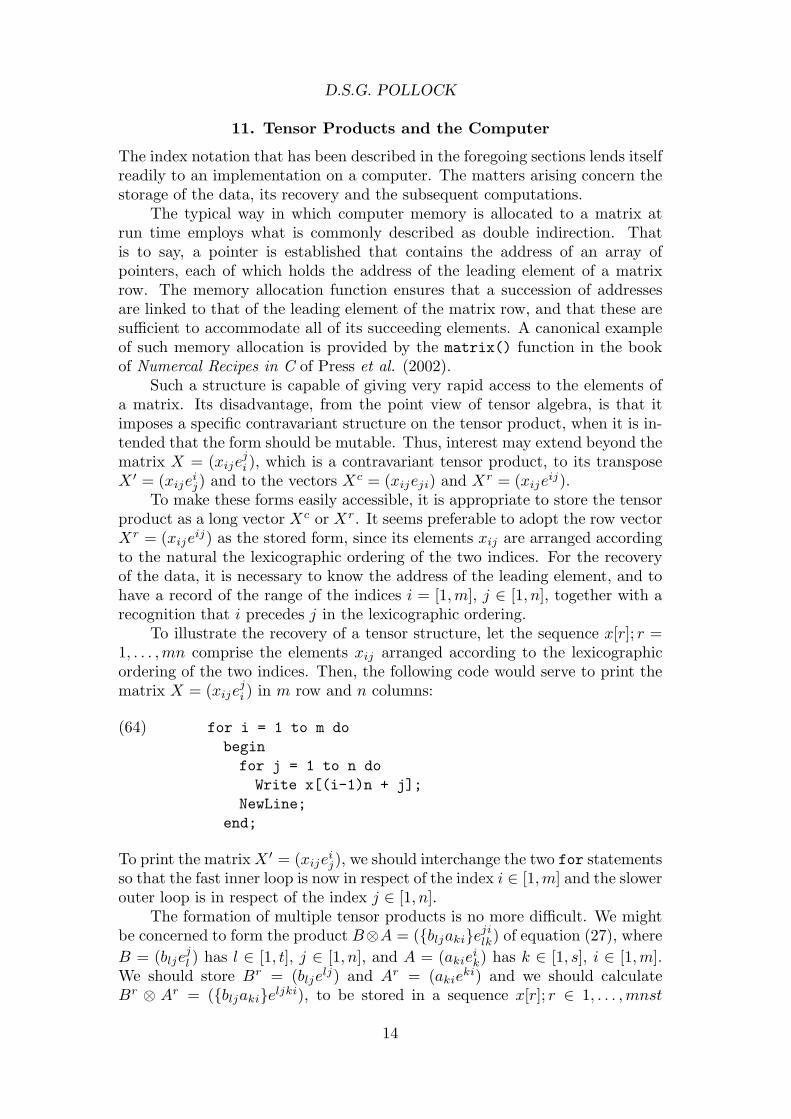
11. Tensor Products and the Computer

The index notation that has been described in the foregoing sections lends itselfreadily to an implementation on a computer. The matters arising concern thestorage of the data, its recovery and the subsequent computations.

The typical way in which computer memory is allocated to a matrix atrun time employs what is commonly described as double indirection. Thatis to say, a pointer is established that contains the address of an array ofpointers, each of which holds the address of the leading element of a matrixrow. The memory allocation function ensures that a succession of addressesare linked to that of the leading element of the matrix row, and that these aresufficient to accommodate all of its succeeding elements. A canonical exampleof such memory allocation is provided by the matrix() function in the bookof Numercal Recipes in C of Press et al. (2002).

Such a structure is capable of giving very rapid access to the elements ofa matrix. Its disadvantage, from the point view of tensor algebra, is that itimposes a specific contravariant structure on the tensor product, when it is in-tended that the form should be mutable. Thus, interest may extend beyond thematrix X = (xije

ji ), which is a contravariant tensor product, to its transpose

X 0 = (xijeij) and to the vectors Xc = (xijeji) and Xr = (xijeij).

To make these forms easily accessible, it is appropriate to store the tensorproduct as a long vector Xc or Xr. It seems preferable to adopt the row vectorXr = (xijeij) as the stored form, since its elements xij are arranged accordingto the natural the lexicographic ordering of the two indices. For the recoveryof the data, it is necessary to know the address of the leading element, and tohave a record of the range of the indices i = [1,m], j ∈ [1, n], together with arecognition that i precedes j in the lexicographic ordering.

To illustrate the recovery of a tensor structure, let the sequence x[r]; r =1, . . . ,mn comprise the elements xij arranged according to the lexicographicordering of the two indices. Then, the following code would serve to print thematrix X = (xije

ji ) in m row and n columns:

(64) for i = 1 to m dobeginfor j = 1 to n doWrite x[(i-1)n + j];

NewLine;end;

To print the matrix X 0 = (xijeij), we should interchange the two for statements

so that the fast inner loop is now in respect of the index i ∈ [1,m] and the slowerouter loop is in respect of the index j ∈ [1, n].

The formation of multiple tensor products is no more difficult. We mightbe concerned to form the product B⊗A = ({bljaki}eji

lk) of equation (27), whereB = (blje

jl ) has l ∈ [1, t], j ∈ [1, n], and A = (akiei

k) has k ∈ [1, s], i ∈ [1,m].We should store Br = (bljelj) and Ar = (akieki) and we should calculateBr ⊗ Ar = ({bljaki}eljki), to be stored in a sequence x[r]; r ∈ 1, . . . ,mnst

14


according to the lexicographic ordering of the indices ljki. Then, the followingcode would serve to print the matrix B ⊗A of st rows and mn columns:

(65) for l = 1 to t dofor k = 1 to s dobeginfor j = 1 to n dofor i = 1 to m doWrite x[(l-1)msn + (j-1)ms + (k-1)m + i];

NewLine;end;

To understand this code, we may note that the composite index

(66)r = [(l − 1)msn + (j − 1)ms + (k − 1)m + i]

= [{(l − 1)n + (j − 1)}s + (k − 1)]m + i

reflects the ordering of the indices ljki, and that it is in accordance with thesequence in which the matrix elements are stored. We may also note that thealternative ordering of the indices lkji, which are associated with the nested forstatements, corresponds to the order of the indices of (B⊗A)r = ({bljaki}elkji)which, disregarding the breaks occasioned by the NewLine statement, is theorder in which we desire to print the elements.

Example. A further example may serve to reaffirm the usefulness of the simpletensor algebra and to hint at the problems in computing to which it can beapplied. The example concerns the mapping from the graphics memory of acomputer to its monitor.

Consider the case of a personal computer of the 1980’s, of which the mon-itor was intended primarily for a textual display. The textual symbols wereformed within character cells that were grids of pixels in eight rows and eightcolumns. The pixel rows may be indexed by k ∈ [1, h] and the pixel columnsmay be indexed by l ∈ [1, w]. Then, the generic lighted pixel can be representedby the matrix el

k, which has a unit in the kth row and the lth column and zeroselsewhere.

In the monitor, there were 40 character cells per line of text, and there were25 lines. The character lines may be indexed by i ∈ [1,m] and the charactercolumns by j ∈ [1, n]. The generic character cell may be represented by thematrix ej

i , which serves to indicate the location of the cell within the contextof the entire screen.

The location of an individual pixel within the screen can be representedby the Kronecker matrix product ej

i ⊗ elk = ejl

ik; and the contents of the screenmay be represented by X = (xijkle

jlik). With 1000 character cells and with 64

bits devoted to each character, the computer’s monochrome graphics memoryamounted to 64,000 bits, albeit that a variety of colours were also available,which added an extra dimension to the tensorial structure. The total memory

15

D.S.G. POLLOCK

of the computer was 64 kilobytes. This dimension determined the name of thecomputer, which was called the Commodore 64—see Jarrett (1984).

Within the computer’s memory, the graphical bits were numbered in asingle sequence beginning with the first bit in the first character cell in the topleft corner of the screen. The sequence passed from the final bit in the firstcharacter cell (number 64 in the lower right corner) to the first bit of the secondcharacter of the line. Thereafter, it passed through successive characters of theline. When the end of the line was reached, the sequence passed to the linebelow.

It follows that the operation that maps the matrix of the pixels of thecomputer console into the bits of the graphics memory can be represented asfollows:

(67) (xijklejlik) −→ (xijkle

ijkl).

The memory location of the generic pixel xijkl is indexed by

(68) r = (i− 1)whn + (j − 1)wh + (k − 1)w + l.

The computer could also be used for plotting scientific graphs. The prob-lem was how to find, within the graphics memory, a pixel that had the screencoordinates (x, y), where x ∈ [1, 320] is a number of pixels representing thehorizontal location, measured from the left edge of the screen, and y ∈ [1, 200]is the vertical location in terms of a pixel count starting from the top of thescreen. This is a matter of finding the indices i, j, k and l that correspond to thecoordinates x and y. Once the indices have been found, the function r(i, j, k, l)of (68) could be used to find the memory location.

The two row indices i and k are obtained from the vertical coordinate yusing the identity

(69)y = h× (y div h) + (y mod h)

= h× (i− 1) + k,

which gives

(70) i = (y div h) + 1 and k = (y mod h).

The column indices j and l are obtained from the horizontal coordinate x usingthe identity

(71)x = w × (x div w) + (x mod w)

= w × (j − 1) + l,

which gives

(72) j = (x div w) + 1 and l = (x mod w).

16


References

Abadir, K.M., and J.R. Magnus, (2005), Matrix Algebra, Cambridge UniversityPress, Cambridge.

Balestra, P., (1976), La Derivation Matricielle, Editions Sirey, Paris.

Bourbaki, N, (1958), Algebre multilineaire, in Elements de Mathematique, BookII (Algebre), Herman, Paris, Chapter 3.

Cartan, E., (1952), Geometrie des Espaces de Riemann, Gauthier–Villars,Paris.

Dwyer, P.S., (1967), Some Applications of Matrix Derivatives in MultivariateAnalysis, Journal of the American Statistical Association, 62, 607–625.

Dwyer, P.S., and M.S. MacPhail, (1948), Symbolic Matrix Derivatives, Annalsof Mathematical Statistics, 19, 517–534.

Graham, A., (1981), Kronecker Products and Matrix Calculus with Applica-tions, Ellis Horwood, Chichester.

Greene, W.H., (2000), Econometric Analysis: Fourth Edition, Prentice-Hall,New Jersey.

Greub, W.H., (1967), Multilinear Algebra, Springer-Verlag, Berlin.

Harville, D.A., (2008), Matrix Algebra from a Statistician’s Perspective,Springer-Verlag, New York.

Henderson, H.V., and S.R. Searle, (1979), Vec and Vech Operators for Matrices,with Some Uses in Jacobians and Multivariate Statistics, The Canadian Journalof Statistics, 7, 65–81.

Henderson, H.V., F. Pukelsheim and S.R. Searle, (1983), On the history of theKronecker Product, Linear and Multilinear Algebra, 14, 13–120.

Jarrett, D., (1984), The Complete Commodore 64, Hutchinson and Co., Lon-don.

Magnus, J.R., (2010), On the Concept of Matrix Derivative, Journal of Multi-variate Analysis, 101, 2200–2206.

Magnus, J.R., and H. Neudecker, (1979), The Commutation Matrix: SomeProperties and Applications, Annals of Statistics, 7, 381–394.

Magnus, J.R., and H. Neudecker, (1988), Matrix Differential Calculus withApplications in Statistics and Econometrics, John Wiley and Sons, Chichester.

Marcus, M., (1973), Finite Dimensional Multilinear Algebra: Part I, MarcelDekker, New York.

Pollock, D.S.G., (1979), The Algebra of Econometrics, John Wiley and Sons,Chichester.

17

D.S.G. POLLOCK

Press, W.H., S.A. Teukolsky, W.T. Vetterling and B.P. Flannery (2002),Numerical Recipes in C: The Art of Scientific Computing, Second Edition,Cambridge University Press, Cambridge.

Rogers, G.S., (1980), Matrix Derivatives, Marcel Dekker, New York.

Theil, H., (1971), Principles of Econometrics, John Wiley and Sons, New York.

Turkington, D.A., (2000), Generalised vec Operators and the Seemingly Unre-lated Regression Equations Model with Vector Correlated Disturbances, Jour-nal of Econometrics, 99, 225–253.

Turkington, D.A., (2002), Matrix Calculus and Zero-One Matrices, CambridgeUniversity Press, Cambridge.

18

on kronecker products, tensor products and matrix ... · tensor products and matrix derivatives...

Documents