on improving distributed pregel-like graph processing systems
TRANSCRIPT
On Improving Distributed Pregel-likeGraph Processing Systems
by
Minyang Han
A thesispresented to the University of Waterloo
in fulfillment of thethesis requirement for the degree of
Master of Mathematicsin
Computer Science
Waterloo, Ontario, Canada, 2015
c© Minyang Han 2015

I hereby declare that I am the sole author of this thesis. This is a true copy of the thesis,including any required final revisions, as accepted by my examiners.
I understand that my thesis may be made electronically available to the public.
ii
Abstract
The considerable interest in distributed systems that can execute algorithms to processlarge graphs has led to the creation of many graph processing systems. However, existingsystems suffer from two major issues: (1) poor performance due to frequent global syn-chronization barriers and limited scalability; and (2) lack of support for graph algorithmsthat require serializability, the guarantee that parallel executions of an algorithm producethe same results as some serial execution of that algorithm.
Many graph processing systems use the bulk synchronous parallel (BSP) model, whichallows graph algorithms to be easily implemented and reasoned about. However, BSPsuffers from poor performance due to stale messages and frequent global synchronizationbarriers. While asynchronous models have been proposed to alleviate these overheads,existing systems that implement such models have limited scalability or retain frequentglobal barriers and do not always support graph mutations or algorithms with multiplecomputation phases. We propose barrierless asynchronous parallel (BAP), a new compu-tation model that overcomes the limitations of existing asynchronous models by reducingboth message staleness and global synchronization while retaining support for graph mu-tations and algorithms with multiple computation phases. We present GiraphUC, whichimplements our BAP model in the open source distributed graph processing system Gi-raph, and evaluate it at scale to demonstrate that BAP provides efficient and transparentasynchronous execution of algorithms that are programmed synchronously.
Secondly, very few systems provide serializability, despite the fact that many graph al-gorithms require it for accuracy, correctness, or termination. To address this deficiency, weprovide a complete solution that can be implemented on top of existing graph processingsystems to provide serializability. Our solution formalizes the notion of serializability andthe conditions under which it can be provided for graph processing systems. We proposea partition-based synchronization technique that enforces these conditions efficiently toprovide serializability. We implement this technique into Giraph and GiraphUC to demon-strate that it is configurable, transparent to algorithm developers, and more performantthan existing techniques.
iii
Acknowledgements
I owe much thanks to my supervisor Khuzaima Daudjee, whose careful guidance andscrupulous attention to detail both sharpened my communication skills and made thisthesis possible. I am also grateful to my readers Tamer Ozsu and Ihab Ilyas for theirinsightful questions and comments. Finally, I’d like to thank colleagues, both IQC andDB, as well as my family and friends for their support during my time at Waterloo.
iv
Table of Contents
List of Tables x
List of Figures xi
1 Introduction 1
1.1 Performance . . . . . . . . . . . . . . . . . . . . . . . . . . . . . . . . . . . 2
1.2 Serializability . . . . . . . . . . . . . . . . . . . . . . . . . . . . . . . . . . 3
1.3 Thesis Outline . . . . . . . . . . . . . . . . . . . . . . . . . . . . . . . . . . 5
2 Related Work 6
2.1 Existing Computation Models . . . . . . . . . . . . . . . . . . . . . . . . . 6
2.1.1 BSP Model . . . . . . . . . . . . . . . . . . . . . . . . . . . . . . . 6
2.1.2 AP Model . . . . . . . . . . . . . . . . . . . . . . . . . . . . . . . . 7
2.1.3 GAS Model . . . . . . . . . . . . . . . . . . . . . . . . . . . . . . . 8
2.2 Categorization . . . . . . . . . . . . . . . . . . . . . . . . . . . . . . . . . . 9
2.2.1 Programming Models . . . . . . . . . . . . . . . . . . . . . . . . . . 10
2.2.2 Computation Models . . . . . . . . . . . . . . . . . . . . . . . . . . 11
2.2.2.1 Synchrony . . . . . . . . . . . . . . . . . . . . . . . . . . . 11
2.2.2.2 Push vs. Pull . . . . . . . . . . . . . . . . . . . . . . . . . 12
2.2.2.3 Global Barriers . . . . . . . . . . . . . . . . . . . . . . . . 12
2.2.2.4 Serializability . . . . . . . . . . . . . . . . . . . . . . . . . 13
v
2.2.3 Additional System Features . . . . . . . . . . . . . . . . . . . . . . 13
2.2.3.1 Graph Partitioning . . . . . . . . . . . . . . . . . . . . . . 13
2.2.3.2 Message Optimizations . . . . . . . . . . . . . . . . . . . . 15
2.2.3.3 Algorithmic Support . . . . . . . . . . . . . . . . . . . . . 17
2.3 Pregel-like Graph Processing Systems . . . . . . . . . . . . . . . . . . . . . 20
2.4 Other Related Systems . . . . . . . . . . . . . . . . . . . . . . . . . . . . . 21
3 Giraph Unchained: Barrierless Asynchronous Parallel Execution 23
3.1 Motivation . . . . . . . . . . . . . . . . . . . . . . . . . . . . . . . . . . . . 23
3.1.1 Performance . . . . . . . . . . . . . . . . . . . . . . . . . . . . . . . 23
3.1.2 Algorithmic Support . . . . . . . . . . . . . . . . . . . . . . . . . . 25
3.2 The BAP Model . . . . . . . . . . . . . . . . . . . . . . . . . . . . . . . . 26
3.2.1 Local Barriers . . . . . . . . . . . . . . . . . . . . . . . . . . . . . . 27
3.2.1.1 Naive Approach . . . . . . . . . . . . . . . . . . . . . . . . 28
3.2.1.2 Improved Approach . . . . . . . . . . . . . . . . . . . . . 28
3.2.2 Algorithmic Support . . . . . . . . . . . . . . . . . . . . . . . . . . 30
3.2.3 Multiple Computation Phases . . . . . . . . . . . . . . . . . . . . . 31
3.3 GiraphUC . . . . . . . . . . . . . . . . . . . . . . . . . . . . . . . . . . . . 32
3.3.1 Giraph Background . . . . . . . . . . . . . . . . . . . . . . . . . . . 33
3.3.2 Giraph Async . . . . . . . . . . . . . . . . . . . . . . . . . . . . . . 34
3.3.3 Adding Local Barriers . . . . . . . . . . . . . . . . . . . . . . . . . 35
3.3.4 Graph Mutations . . . . . . . . . . . . . . . . . . . . . . . . . . . . 35
3.3.5 Multiple Computation Phases . . . . . . . . . . . . . . . . . . . . . 36
3.3.5.1 Giraph Async . . . . . . . . . . . . . . . . . . . . . . . . . 37
3.3.6 Aggregators and Combiners . . . . . . . . . . . . . . . . . . . . . . 37
3.3.7 Fault Tolerance . . . . . . . . . . . . . . . . . . . . . . . . . . . . . 37
3.4 Experimental Evaluation . . . . . . . . . . . . . . . . . . . . . . . . . . . . 38
3.4.1 Experimental Setup . . . . . . . . . . . . . . . . . . . . . . . . . . . 38
vi

3.4.2 Algorithms . . . . . . . . . . . . . . . . . . . . . . . . . . . . . . . 39
3.4.2.1 SSSP . . . . . . . . . . . . . . . . . . . . . . . . . . . . . 40
3.4.2.2 WCC . . . . . . . . . . . . . . . . . . . . . . . . . . . . . 41
3.4.2.3 DMST . . . . . . . . . . . . . . . . . . . . . . . . . . . . . 41
3.4.2.4 PageRank . . . . . . . . . . . . . . . . . . . . . . . . . . . 42
3.4.3 Results . . . . . . . . . . . . . . . . . . . . . . . . . . . . . . . . . . 43
3.4.3.1 SSSP . . . . . . . . . . . . . . . . . . . . . . . . . . . . . 43
3.4.3.2 WCC . . . . . . . . . . . . . . . . . . . . . . . . . . . . . 45
3.4.3.3 DMST . . . . . . . . . . . . . . . . . . . . . . . . . . . . . 45
3.4.3.4 PageRank . . . . . . . . . . . . . . . . . . . . . . . . . . . 46
3.4.4 Sensitivity Analysis . . . . . . . . . . . . . . . . . . . . . . . . . . . 47
3.4.4.1 Message Batching . . . . . . . . . . . . . . . . . . . . . . 47
3.4.4.2 Local Barriers . . . . . . . . . . . . . . . . . . . . . . . . . 48
3.5 Summary . . . . . . . . . . . . . . . . . . . . . . . . . . . . . . . . . . . . 49
4 Providing Serializability 50
4.1 Motivation . . . . . . . . . . . . . . . . . . . . . . . . . . . . . . . . . . . . 50
4.1.1 BSP Model . . . . . . . . . . . . . . . . . . . . . . . . . . . . . . . 50
4.1.2 AP Model . . . . . . . . . . . . . . . . . . . . . . . . . . . . . . . . 51
4.1.3 BAP Model . . . . . . . . . . . . . . . . . . . . . . . . . . . . . . . 51
4.1.4 GAS Model . . . . . . . . . . . . . . . . . . . . . . . . . . . . . . . 52
4.2 Serializability . . . . . . . . . . . . . . . . . . . . . . . . . . . . . . . . . . 52
4.2.1 Preliminaries . . . . . . . . . . . . . . . . . . . . . . . . . . . . . . 52
4.2.2 Transactions . . . . . . . . . . . . . . . . . . . . . . . . . . . . . . . 54
4.2.3 Replicated Data . . . . . . . . . . . . . . . . . . . . . . . . . . . . . 54
4.2.4 Correctness . . . . . . . . . . . . . . . . . . . . . . . . . . . . . . . 55
4.2.5 Enforcing Serializability . . . . . . . . . . . . . . . . . . . . . . . . 58
4.3 Synchronization Techniques . . . . . . . . . . . . . . . . . . . . . . . . . . 59
vii
4.3.1 Preliminaries . . . . . . . . . . . . . . . . . . . . . . . . . . . . . . 59
4.3.1.1 Replica Updates . . . . . . . . . . . . . . . . . . . . . . . 59
4.3.1.2 Architectural Considerations . . . . . . . . . . . . . . . . 60
4.3.2 Token Passing . . . . . . . . . . . . . . . . . . . . . . . . . . . . . . 60
4.3.2.1 Single-Layer Token Passing . . . . . . . . . . . . . . . . . 60
4.3.2.2 Dual-Layer Token Passing . . . . . . . . . . . . . . . . . . 61
4.3.2.3 Discussion . . . . . . . . . . . . . . . . . . . . . . . . . . . 62
4.3.3 Partition-based Distributed Locking . . . . . . . . . . . . . . . . . . 63
4.3.3.1 Vertex-based Distributed Locking . . . . . . . . . . . . . . 64
4.3.3.2 Discussion . . . . . . . . . . . . . . . . . . . . . . . . . . . 65
4.4 Implementation . . . . . . . . . . . . . . . . . . . . . . . . . . . . . . . . . 65
4.4.1 Giraph Background . . . . . . . . . . . . . . . . . . . . . . . . . . . 66
4.4.2 Dual-Layer Token Passing . . . . . . . . . . . . . . . . . . . . . . . 66
4.4.3 Partition-based Distributed Locking . . . . . . . . . . . . . . . . . . 67
4.4.4 Vertex-Based Distributed Locking . . . . . . . . . . . . . . . . . . . 68
4.4.5 Fault Tolerance . . . . . . . . . . . . . . . . . . . . . . . . . . . . . 69
4.4.6 Algorithmic Compatibility and Usability . . . . . . . . . . . . . . . 69
4.5 Experimental Evaluation . . . . . . . . . . . . . . . . . . . . . . . . . . . . 70
4.5.1 Experimental Setup . . . . . . . . . . . . . . . . . . . . . . . . . . . 70
4.5.2 Algorithms . . . . . . . . . . . . . . . . . . . . . . . . . . . . . . . 71
4.5.2.1 Graph Coloring . . . . . . . . . . . . . . . . . . . . . . . . 72
4.5.3 Results . . . . . . . . . . . . . . . . . . . . . . . . . . . . . . . . . . 73
4.6 Summary . . . . . . . . . . . . . . . . . . . . . . . . . . . . . . . . . . . . 74
5 Conclusion 75
5.1 Future Work . . . . . . . . . . . . . . . . . . . . . . . . . . . . . . . . . . . 76
5.1.1 Globally Coordinated Aggregators . . . . . . . . . . . . . . . . . . . 76
5.1.2 Generalized Serializability . . . . . . . . . . . . . . . . . . . . . . . 77
5.1.3 Asynchronous Models in Generic Systems . . . . . . . . . . . . . . 78
viii

APPENDICES 79
A Proofs for Giraph Unchained 80
A.1 Preliminaries . . . . . . . . . . . . . . . . . . . . . . . . . . . . . . . . . . 80
A.1.1 Type A . . . . . . . . . . . . . . . . . . . . . . . . . . . . . . . . . 82
A.1.2 Type B . . . . . . . . . . . . . . . . . . . . . . . . . . . . . . . . . 82
A.2 Theorem 1 . . . . . . . . . . . . . . . . . . . . . . . . . . . . . . . . . . . . 83
A.3 Theorem 2 . . . . . . . . . . . . . . . . . . . . . . . . . . . . . . . . . . . . 84
References 86
ix
List of Tables
2.1 Algorithmic requirements for graph processing and machine learning algo-rithms. . . . . . . . . . . . . . . . . . . . . . . . . . . . . . . . . . . . . . . 16
2.2 Categorization of Pregel-like graph processing systems based on their corefeatures. . . . . . . . . . . . . . . . . . . . . . . . . . . . . . . . . . . . . . 18
2.3 Categorization of Pregel-like graph processing systems based on their addi-tional features. . . . . . . . . . . . . . . . . . . . . . . . . . . . . . . . . . 19
3.1 Directed datasets. Parentheses indicate values for the undirected versionsused by DMST. . . . . . . . . . . . . . . . . . . . . . . . . . . . . . . . . . 38
4.1 Directed datasets. Parentheses give values for the undirected versions usedby graph coloring. . . . . . . . . . . . . . . . . . . . . . . . . . . . . . . . . 71
x
List of Figures
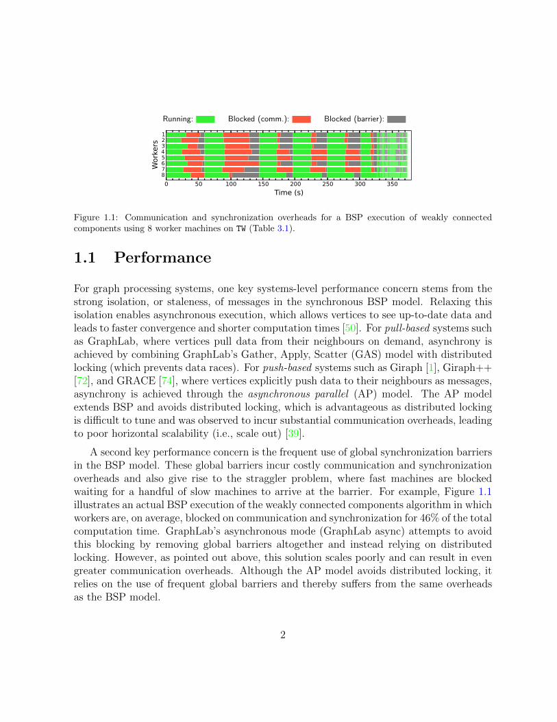
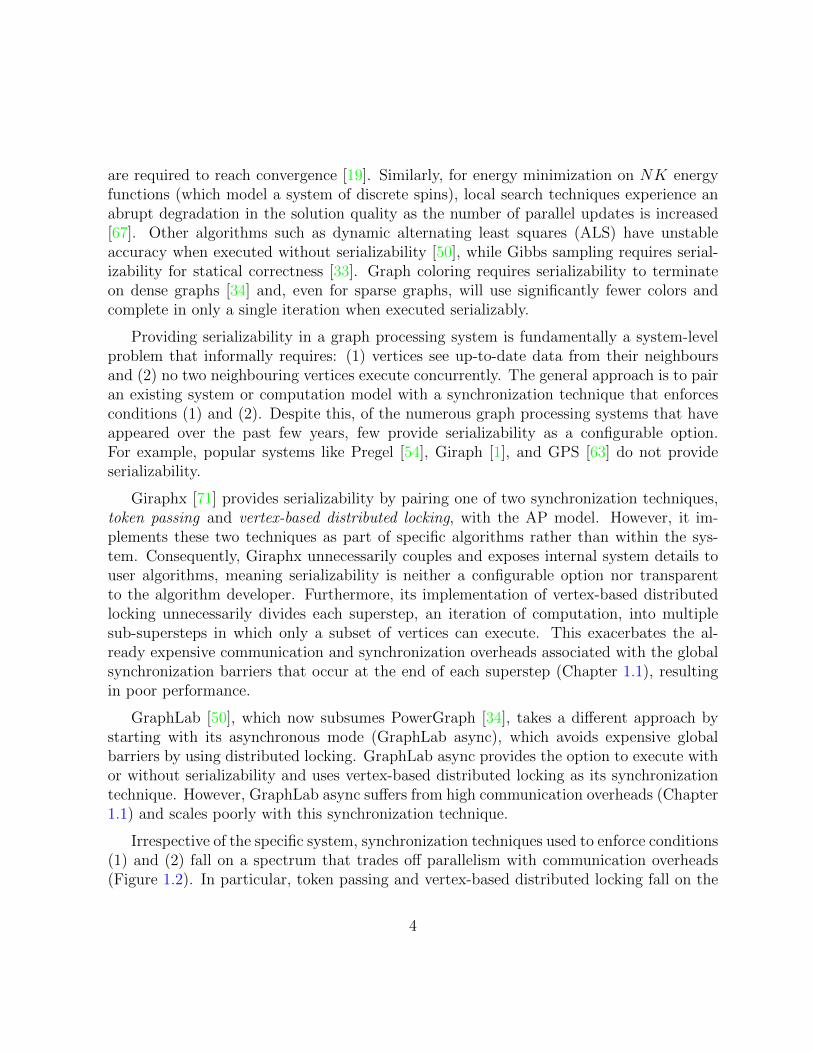
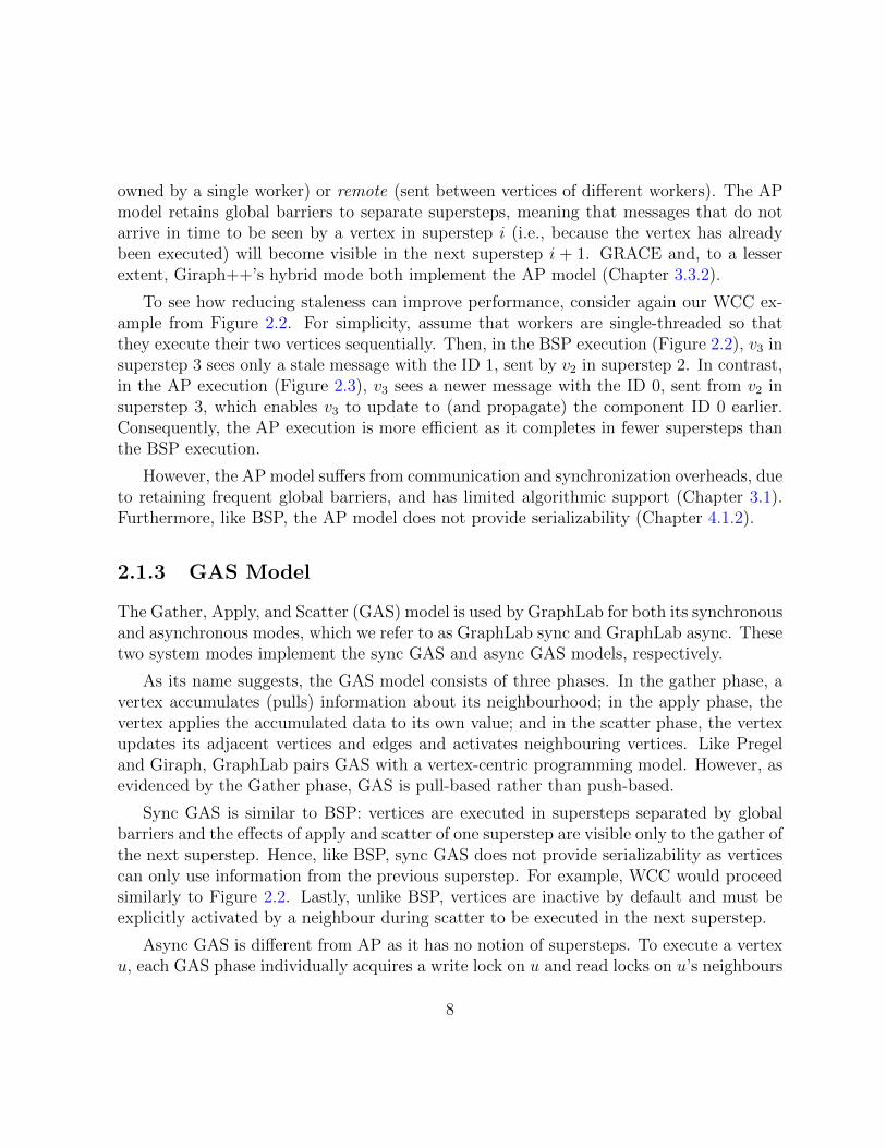
1.1 Communication and synchronization overheads for a BSP execution of weaklyconnected components using 8 worker machines on TW (Table 3.1). . . . . . 2
1.2 Spectrum of synchronization techniques. . . . . . . . . . . . . . . . . . . . 5
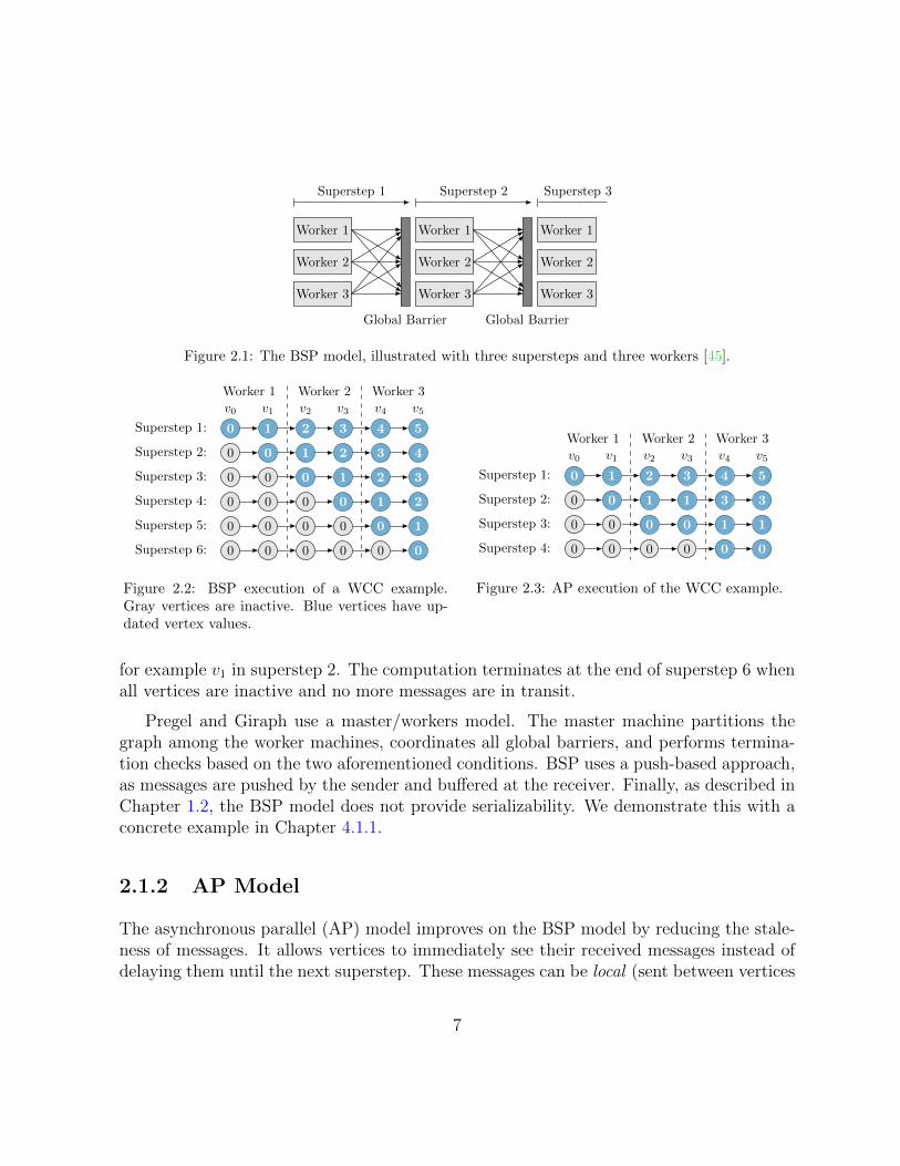
2.1 The BSP model, illustrated with three supersteps and three workers [45]. . 7
2.2 BSP execution of a WCC example. Gray vertices are inactive. Blue verticeshave updated vertex values. . . . . . . . . . . . . . . . . . . . . . . . . . . 7
2.3 AP execution of the WCC example. . . . . . . . . . . . . . . . . . . . . . . 7
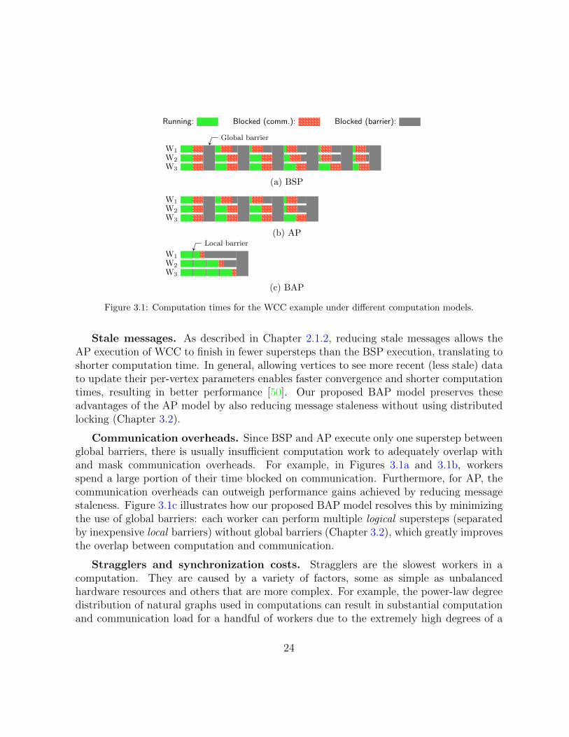
3.1 Computation times for the WCC example under different computation models. 24
3.2 WCC computation times based on real executions of 16 workers on TW (Table3.1). . . . . . . . . . . . . . . . . . . . . . . . . . . . . . . . . . . . . . . . 25
3.3 The BAP model, with two global supersteps and three workers. GSS standsfor global superstep, while LSS stands for logical superstep. . . . . . . . . . 26
3.4 Simplified comparison of worker control flows for the two approaches to localbarriers. LSS stands for logical superstep and GB for global barrier. . . . . 28
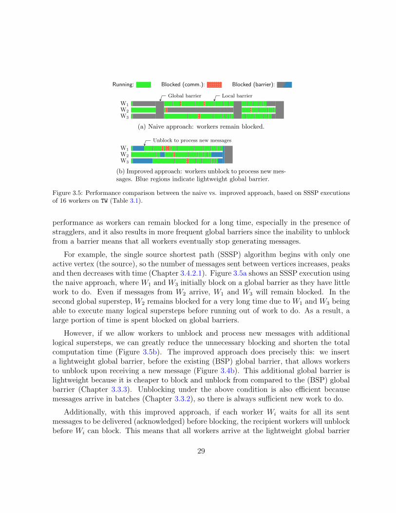
3.5 Performance comparison between the naive vs. improved approach, basedon SSSP executions of 16 workers on TW (Table 3.1). . . . . . . . . . . . . . 29
3.6 Computation times for SSSP, WCC, and DMST. Missing bars are labelledwith ‘F’ for unsuccessful runs and ‘NS’ for unsupported algorithms. . . . . 44
3.7 Plots of L1-norm (error) vs. computation time for PageRank. . . . . . . . . 46
3.8 Computation times for SSSP and WCC in GiraphUC with different buffercache sizes. . . . . . . . . . . . . . . . . . . . . . . . . . . . . . . . . . . . 48
xi
3.9 Computation times for SSSP and WCC using naive vs. improved approachto local barriers. . . . . . . . . . . . . . . . . . . . . . . . . . . . . . . . . . 49
4.1 BSP execution of greedy graph coloring. Each graph is the state at the endof that superstep. . . . . . . . . . . . . . . . . . . . . . . . . . . . . . . . . 51
4.2 AP execution of greedy graph coloring. Each graph is the state at the endof that superstep. . . . . . . . . . . . . . . . . . . . . . . . . . . . . . . . . 51
4.3 Computation times for graph coloring, PageRank, SSSP, and WCC. Missingbars are labelled with ‘F’ for unsuccessful runs. . . . . . . . . . . . . . . . 74
xii
Chapter 1
Introduction
Due to the wide variety of real-world problems that rely on processing large amounts ofgraph data, graph data processing has become ubiquitous. For example, web graphs con-taining over 60 trillion indexed webpages must be processed by Google’s ranking algorithmsto determine influential vertices [35]. Massive social graphs are processed at Facebook tocompute popularity and personalized rankings, determine shared connections, find commu-nities, and propagate advertisements for over 1 billion monthly active users [30]. Scientistsare also leveraging biology graphs to understand protein interactions [58] and cell graphsfor automated cancer diagnosis [37].
Graph processing solves real-world problems through graph algorithms that are imple-mented and executed on graph processing systems. These systems provide programmingand computation models, which developers use to implement such algorithms, as well asany correctness guarantees that algorithms require. The systems are also used to executealgorithms against desired input graphs.
Google’s Pregel [54] is one such system that provides a native graph processing API bypairing the bulk synchronous parallel (BSP) computation model [73] with a vertex-centric,or “think like a vertex”, programming model. This has inspired many popular open sourcePregel-like graph processing systems, including Apache Giraph [1] and GraphLab [50].
However, these Pregel-like systems suffer from two major issues: (1) poor performanceat scale due to the frequent use of global synchronization barriers and (2) a lack of serial-izability guarantees for graph algorithms.
1
Running: Blocked (comm.): Blocked (barrier):
0 50 100 150 200 250 300 350
Time (s)
87654321
Workers
Figure 1.1: Communication and synchronization overheads for a BSP execution of weakly connectedcomponents using 8 worker machines on TW (Table 3.1).
1.1 Performance
For graph processing systems, one key systems-level performance concern stems from thestrong isolation, or staleness, of messages in the synchronous BSP model. Relaxing thisisolation enables asynchronous execution, which allows vertices to see up-to-date data andleads to faster convergence and shorter computation times [50]. For pull-based systems suchas GraphLab, where vertices pull data from their neighbours on demand, asynchrony isachieved by combining GraphLab’s Gather, Apply, Scatter (GAS) model with distributedlocking (which prevents data races). For push-based systems such as Giraph [1], Giraph++[72], and GRACE [74], where vertices explicitly push data to their neighbours as messages,asynchrony is achieved through the asynchronous parallel (AP) model. The AP modelextends BSP and avoids distributed locking, which is advantageous as distributed lockingis difficult to tune and was observed to incur substantial communication overheads, leadingto poor horizontal scalability (i.e., scale out) [39].
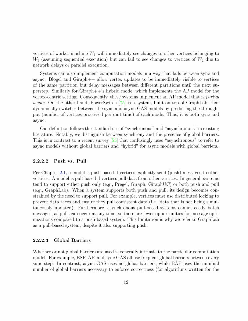
A second key performance concern is the frequent use of global synchronization barriersin the BSP model. These global barriers incur costly communication and synchronizationoverheads and also give rise to the straggler problem, where fast machines are blockedwaiting for a handful of slow machines to arrive at the barrier. For example, Figure 1.1illustrates an actual BSP execution of the weakly connected components algorithm in whichworkers are, on average, blocked on communication and synchronization for 46% of the totalcomputation time. GraphLab’s asynchronous mode (GraphLab async) attempts to avoidthis blocking by removing global barriers altogether and instead relying on distributedlocking. However, as pointed out above, this solution scales poorly and can result in evengreater communication overheads. Although the AP model avoids distributed locking, itrelies on the use of frequent global barriers and thereby suffers from the same overheadsas the BSP model.
2
Finally, there is a third concern of usability and also compatibility. The simple anddeterministic nature of the BSP model enables algorithm developers to easily reason about,and debug, their code. In contrast, a fully exposed asynchronous model requires carefulconsideration of the underlying consistency guarantees as well as coding and debugging ina non-deterministic setting, both of which can be confusing and lead to buggy code. Hence,a performant graph processing system should allow developers to code for the BSP modeland transparently execute with an efficient asynchronous computation model. Existingsystems that provide asynchronous execution leak too much of the underlying asynchronousmechanisms to the developer API [74], impeding usability, and do not support algorithmsthat require graph mutations [50, 74] or algorithms with multiple computation phases [72],impeding compatibility.
To address these concerns, we propose a barrierless asynchronous parallel (BAP) com-putation model that both relaxes message isolation and substantially reduces the frequencyof global barriers, without using distributed locking. Our system, GiraphUC, implementsthe proposed BAP model in Giraph, a popular open source system. GiraphUC preservesGiraph’s BSP developer interface and fully supports algorithms that perform graph muta-tions or have multiple computation phases. GiraphUC is also more scalable than GraphLabasync and achieves good performance improvements over Giraph, Giraph async (which usesthe AP model), and GraphLab sync and async. Thus, GiraphUC enables developers tocode for a synchronous BSP model and transparently execute with an asynchronous BAPmodel to maximize performance.
1.2 Serializability
A key guarantee that graph processing systems can provide is serializability. Informally, agraph processing system provides serializability if it can guarantee that parallel executionsof an algorithm, implemented with its programming and computation models, produce thesame results as some serial execution of that algorithm [34].
Serializability is required by many algorithms, for example in machine learning, to pro-vide both theoretical and empirical guarantees for convergence or termination. Parallelalgorithms for combinatorial optimization problems experience a drop in performance andaccuracy when parallelism is increased without consideration for serializability. For ex-ample, the Shotgun algorithm for L1-regularized loss minimization parallelizes sequentialcoordinate descent to handle problems with high dimensionality or large sample sizes [19].As the number of parallel updates is increased, convergence is achieved in fewer iterations.However, after a sufficient amount of parallelism, divergence occurs and more iterations
3
are required to reach convergence [19]. Similarly, for energy minimization on NK energyfunctions (which model a system of discrete spins), local search techniques experience anabrupt degradation in the solution quality as the number of parallel updates is increased[67]. Other algorithms such as dynamic alternating least squares (ALS) have unstableaccuracy when executed without serializability [50], while Gibbs sampling requires serial-izability for statical correctness [33]. Graph coloring requires serializability to terminateon dense graphs [34] and, even for sparse graphs, will use significantly fewer colors andcomplete in only a single iteration when executed serializably.
Providing serializability in a graph processing system is fundamentally a system-levelproblem that informally requires: (1) vertices see up-to-date data from their neighboursand (2) no two neighbouring vertices execute concurrently. The general approach is to pairan existing system or computation model with a synchronization technique that enforcesconditions (1) and (2). Despite this, of the numerous graph processing systems that haveappeared over the past few years, few provide serializability as a configurable option.For example, popular systems like Pregel [54], Giraph [1], and GPS [63] do not provideserializability.
Giraphx [71] provides serializability by pairing one of two synchronization techniques,token passing and vertex-based distributed locking, with the AP model. However, it im-plements these two techniques as part of specific algorithms rather than within the sys-tem. Consequently, Giraphx unnecessarily couples and exposes internal system details touser algorithms, meaning serializability is neither a configurable option nor transparentto the algorithm developer. Furthermore, its implementation of vertex-based distributedlocking unnecessarily divides each superstep, an iteration of computation, into multiplesub-supersteps in which only a subset of vertices can execute. This exacerbates the al-ready expensive communication and synchronization overheads associated with the globalsynchronization barriers that occur at the end of each superstep (Chapter 1.1), resultingin poor performance.
GraphLab [50], which now subsumes PowerGraph [34], takes a different approach bystarting with its asynchronous mode (GraphLab async), which avoids expensive globalbarriers by using distributed locking. GraphLab async provides the option to execute withor without serializability and uses vertex-based distributed locking as its synchronizationtechnique. However, GraphLab async suffers from high communication overheads (Chapter1.1) and scales poorly with this synchronization technique.
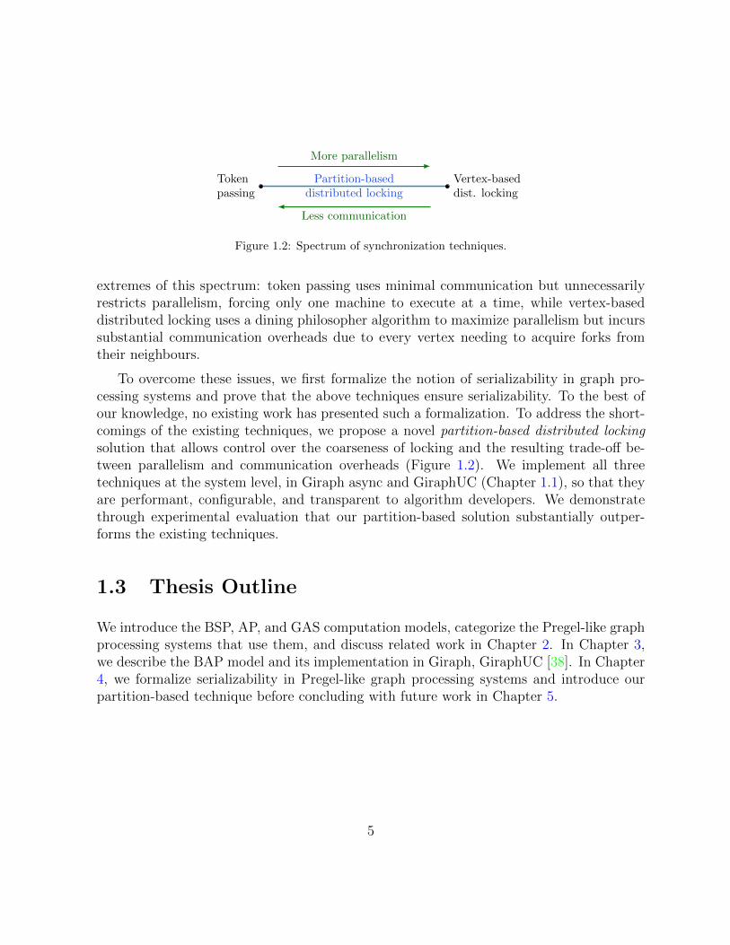
Irrespective of the specific system, synchronization techniques used to enforce conditions(1) and (2) fall on a spectrum that trades off parallelism with communication overheads(Figure 1.2). In particular, token passing and vertex-based distributed locking fall on the
4
More parallelism
Less communication
Tokenpassing
Vertex-baseddist. locking
Partition-baseddistributed locking
Figure 1.2: Spectrum of synchronization techniques.
extremes of this spectrum: token passing uses minimal communication but unnecessarilyrestricts parallelism, forcing only one machine to execute at a time, while vertex-baseddistributed locking uses a dining philosopher algorithm to maximize parallelism but incurssubstantial communication overheads due to every vertex needing to acquire forks fromtheir neighbours.
To overcome these issues, we first formalize the notion of serializability in graph pro-cessing systems and prove that the above techniques ensure serializability. To the best ofour knowledge, no existing work has presented such a formalization. To address the short-comings of the existing techniques, we propose a novel partition-based distributed lockingsolution that allows control over the coarseness of locking and the resulting trade-off be-tween parallelism and communication overheads (Figure 1.2). We implement all threetechniques at the system level, in Giraph async and GiraphUC (Chapter 1.1), so that theyare performant, configurable, and transparent to algorithm developers. We demonstratethrough experimental evaluation that our partition-based solution substantially outper-forms the existing techniques.
1.3 Thesis Outline
We introduce the BSP, AP, and GAS computation models, categorize the Pregel-like graphprocessing systems that use them, and discuss related work in Chapter 2. In Chapter 3,we describe the BAP model and its implementation in Giraph, GiraphUC [38]. In Chapter4, we formalize serializability in Pregel-like graph processing systems and introduce ourpartition-based technique before concluding with future work in Chapter 5.
5
Chapter 2
Related Work
We begin by introducing the BSP, AP, and GAS computation models in Chapter 2.1,followed by a categorization of Pregel-like graph processing systems in Chapter 2.2, andconclude with a discussion on some additional systems related to graph processing.
2.1 Existing Computation Models
2.1.1 BSP Model
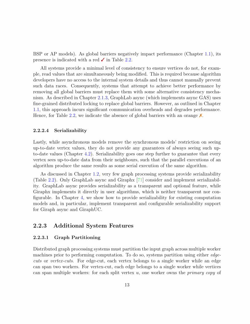
Bulk synchronous parallel (BSP) [73] is a parallel computation model in which computa-tions are divided into a series of (BSP) supersteps separated by global barriers (Figure 2.1).To support iterative graph computations, Pregel (and Giraph) pairs BSP with a vertex-centric programming model, in which vertices are the units of computation and edges actas communication channels between vertices.
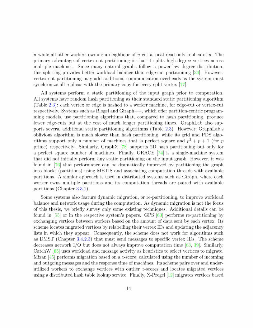
Graph computations are specified by a user-defined compute function that executes,in parallel, on all vertices in each superstep. Consider, as a running example, the BSPexecution of the weakly connected components (WCC) algorithm (Figure 2.2). In the firstsuperstep, each vertex initializes its vertex value to a component ID. In the subsequentsupersteps, it updates this value with any smaller IDs received from its in-edge neighboursand propagates any changes along its out-edges (Chapter 3.4.2.2). Crucially, messagessent in one superstep are visible only during the next superstep. For example, ID 1 sentby v2 in superstep 2 is seen by v3 only in superstep 3. At the end of each superstep, allvertices “vote to halt” to become inactive. A vertex is reactivated by incoming messages,
6
Worker 1
Worker 2
Worker 3
Worker 1
Worker 2
Worker 3
Worker 1
Worker 2
Worker 3
Global Barrier Global Barrier
Superstep 1 Superstep 2 Superstep 3
Figure 2.1: The BSP model, illustrated with three supersteps and three workers [45].
Superstep 1:
Superstep 2:
Superstep 3:
Superstep 4:
Superstep 5:
Superstep 6:
0 1 2 3 4 5
v0 v1 v2 v3 v4 v5
Worker 1 Worker 2 Worker 3
0 0 1 2 3 4
0 0 0 1 2 3
0 0 0 0 1 2
0 0 0 0 0 1
0 0 0 0 0 0
Figure 2.2: BSP execution of a WCC example.Gray vertices are inactive. Blue vertices have up-dated vertex values.
Superstep 1:
Superstep 2:
Superstep 3:
Superstep 4:
0 1 2 3 4 5
v0 v1 v2 v3 v4 v5
Worker 1 Worker 2 Worker 3
0 0 1 1 3 3
0 0 0 0 1 1
0 0 0 0 0 0
Figure 2.3: AP execution of the WCC example.
for example v1 in superstep 2. The computation terminates at the end of superstep 6 whenall vertices are inactive and no more messages are in transit.
Pregel and Giraph use a master/workers model. The master machine partitions thegraph among the worker machines, coordinates all global barriers, and performs termina-tion checks based on the two aforementioned conditions. BSP uses a push-based approach,as messages are pushed by the sender and buffered at the receiver. Finally, as described inChapter 1.2, the BSP model does not provide serializability. We demonstrate this with aconcrete example in Chapter 4.1.1.
2.1.2 AP Model
The asynchronous parallel (AP) model improves on the BSP model by reducing the stale-ness of messages. It allows vertices to immediately see their received messages instead ofdelaying them until the next superstep. These messages can be local (sent between vertices
7
owned by a single worker) or remote (sent between vertices of different workers). The APmodel retains global barriers to separate supersteps, meaning that messages that do notarrive in time to be seen by a vertex in superstep i (i.e., because the vertex has alreadybeen executed) will become visible in the next superstep i + 1. GRACE and, to a lesserextent, Giraph++’s hybrid mode both implement the AP model (Chapter 3.3.2).
To see how reducing staleness can improve performance, consider again our WCC ex-ample from Figure 2.2. For simplicity, assume that workers are single-threaded so thatthey execute their two vertices sequentially. Then, in the BSP execution (Figure 2.2), v3 insuperstep 3 sees only a stale message with the ID 1, sent by v2 in superstep 2. In contrast,in the AP execution (Figure 2.3), v3 sees a newer message with the ID 0, sent from v2 insuperstep 3, which enables v3 to update to (and propagate) the component ID 0 earlier.Consequently, the AP execution is more efficient as it completes in fewer supersteps thanthe BSP execution.
However, the AP model suffers from communication and synchronization overheads, dueto retaining frequent global barriers, and has limited algorithmic support (Chapter 3.1).Furthermore, like BSP, the AP model does not provide serializability (Chapter 4.1.2).
2.1.3 GAS Model
The Gather, Apply, and Scatter (GAS) model is used by GraphLab for both its synchronousand asynchronous modes, which we refer to as GraphLab sync and GraphLab async. Thesetwo system modes implement the sync GAS and async GAS models, respectively.
As its name suggests, the GAS model consists of three phases. In the gather phase, avertex accumulates (pulls) information about its neighbourhood; in the apply phase, thevertex applies the accumulated data to its own value; and in the scatter phase, the vertexupdates its adjacent vertices and edges and activates neighbouring vertices. Like Pregeland Giraph, GraphLab pairs GAS with a vertex-centric programming model. However, asevidenced by the Gather phase, GAS is pull-based rather than push-based.
Sync GAS is similar to BSP: vertices are executed in supersteps separated by globalbarriers and the effects of apply and scatter of one superstep are visible only to the gather ofthe next superstep. Hence, like BSP, sync GAS does not provide serializability as verticescan only use information from the previous superstep. For example, WCC would proceedsimilarly to Figure 2.2. Lastly, unlike BSP, vertices are inactive by default and must beexplicitly activated by a neighbour during scatter to be executed in the next superstep.
Async GAS is different from AP as it has no notion of supersteps. To execute a vertexu, each GAS phase individually acquires a write lock on u and read locks on u’s neighbours
8
to prevent data races [8]. GraphLab async implements async GAS by maintaining a largepool of lightweight threads (called fibers) and pairing each fiber with an available vertex.Before executing each GAS phase, the fiber acquires the necessary locks through distributedlocking. To terminate, GraphLab async runs a distributed consensus algorithm to checkthat all workers’ schedulers are empty (i.e., no more vertices to execute).
In contrast, AP can avoid async GAS’s expensive distributed locking because it is push-based: messages are received only after a vertex finishes its computation and explicitlypushes such messages. Since messages are buffered in the recipient machine’s local messagestore, concurrent reads and writes to the store (i.e., data races) can be handled with locallocks or lock-free data structures. Furthermore, the AP model can rely on the master tocheck for termination, which avoids the overheads of a distributed consensus algorithm.
Finally, async GAS does not provide serializability because the GAS phases of differ-ent vertex computations can interleave [34]. To provide serializability (Chapter 4.2.5), asynchronization technique must be added on top of async GAS. This technique preventsneighbouring computations from interleaving by performing vertex-based distributed lock-ing over all three GAS phases. Note that this is different from the per-phase distributedlocking used by async GAS to prevent data races. As we show in Chapter 4.2, async GASprovides serializability when paired with this synchronization technique.
2.2 Categorization
Graph processing systems can be categorized based on their developer API and type ofsystem execution (Table 2.2) as well as general feature support (Table 2.3).
The developer API consists of the programming and computation models that the sys-tem exposes to algorithm developers for creating algorithms. For example, the API ex-posed by Pregel [54] is a vertex-centric programming model paired with a BSP computationmodel.
The type of system execution depends on both the computation model used by thesystem, which may be different from what is exposed by its API, and additional propertiesof the system, some of which are intrinsic to the computation model used. For example, ifthe system uses the BSP model then it must have global barriers, as barriers are intrinsicto BSP. On the other hand, providing serializability is not intrinsic to any computationmodel. Most systems use a computation model that is identical to the one exposed for itsdeveloper API. However, this need not always be the case: GiraphUC, for example, exposes
9
a BSP (or AP) computation model for developers but transparently executes using the BAPcomputation model (Chapter 3.2).
Lastly, a system’s general feature support consists of its graph partitioning and dynamicmigration (re-partitioning) schemes, message optimizations, and support for algorithmsthat perform graph mutations (addition and deletion of vertices and edges) and algorithmswith multiple computation phases (multi-phase algorithms).
We break down and detail programming models, computational models, and each ofthe general feature supports next.
2.2.1 Programming Models
Most systems are vertex-centric (v-centric), following the “think like a vertex” program-ming model used by Pregel and described in Chapter 2.1.1. For example, Giraph [1], GPS[63], GraphLab [50], and GiraphUC are all vertex-centric (Table 2.2).
There are also systems that consider a partition-centric (p-centric) approach, where de-velopers define the execution of each partition of vertices (where each worker machine canhave multiple partitions). For example, in addition to the regular vertex-centric computefunction, Blogel [80] lets developers specify a B-compute function that is executed on eachblock (partition) of vertices. In Giraph++ [72], developers define only a compute functionfor executing partitions of vertices. This improves expressibility by allowing developers toexecute sequential algorithms over the vertices of each partition. However, it negativelyimpacts usability as the algorithms are more complex: since partitions execute in paral-lel, developers must reason about the coordination of each partition’s boundary verticesbecause they must communicate with neighbours that belong to other partitions.
Finally, the single-machine disk-based system X-Stream [62] uses an edge-centric ap-proach: developers define scatter and gather-and-apply functions that are performed onedges rather than vertices. X-Stream uses this to avoid random I/O, which leads to betterperformance because portions of the graph must be streamed from disk back into memoryduring computation. However, the edge-centric approach is less intuitive and is thus notwidely adopted: other single-machine disk-based systems like FlashGraph [86], GraphChi[48], TurboGraph [40], and VENUS [24] all use a vertex-centric programming model. Sinceour focus is on in-memory systems, we exclude these disk-based systems from Tables 2.2and 2.3. They are discussed in Chapter 2.4.
10
2.2.2 Computation Models
Computation models can be broken down and categorized based on their core features.Some of these features are intrinsic to the model (i.e., the model is defined to have it), whileothers are extrinsic and depend on whether the graph processing system implements it.For example, the BSP computation model will, by definition, always have global barriers.In contrast, the GAS model can be implemented either as a synchronous model or as anasynchronous model and thus with or without global barriers.
Computation models have three central pillars: synchrony, push/pull, and global bar-riers. We additionally have an orthogonal but equally important pillar of serializability.Serializability is closely related to synchrony but can be thought of as orthogonal to thecomputation model: one can provide serializability in a model-agnostic manner1 on top ofexisting computation models (Chapter 4.2.5).
While the design choices are targeted to improve system performance independentlyfor each pillar, these choices may also indirectly impact the performance of other pillars.For example, although asynchronous models generally perform better than synchronousmodels, async GAS’s support for a pull-based approach leads to significant communica-tion overheads due to distributed locking (Chapter 2.1.3), ultimately resulting in poorperformance. In the case of providing serializability, asynchronous computation modelscan support a wider range of synchronization techniques, including a more performantpartition-based distributed locking technique (Chapter 1.2), which substantially increasestheir performance advantage over synchronous computation models.
2.2.2.1 Synchrony
As described in Chapters 1.1 and 2.1, a computation model is synchronous (sync) if allupdates of any vertex u in superstep i is visible to other vertices only in superstep i + 1.That is, recipients do not see the messages sent (pushed) by u until superstep i + 1.Equivalently, for pull-based models, vertices do not see an up-to-date value when pullingu’s vertex value.
A model is asynchronous (async) when this is relaxed: i.e., the update of a vertex ucan be seen by other vertices in the same superstep. Importantly, asynchronous models donot guarantee that other vertices will always see an up-to-date vertex u—it only removesthe restriction that says they cannot. For example, in the AP model (Chapter 2.1.2),
1However, synchronous computation models support only a subset of synchronization techniques, whichprovide serializability, whereas asynchronous models have no such limitations (Chapter 4.3.1.1).
11
vertices of worker machine W1 will immediately see changes to other vertices belonging toW1 (assuming sequential execution) but can fail to see changes to vertices of W2 due tonetwork delays or parallel execution.
Systems can also implement computation models in a way that falls between sync andasync. Blogel and Giraph++ allow vertex updates to be immediately visible to verticesof the same partition but delay messages between different partitions until the next su-perstep. Similarly for Giraph++’s hybrid mode, which implements the AP model for thevertex-centric setting. Consequently, these systems implement an AP model that is partialasync. On the other hand, PowerSwitch [75] is a system, built on top of GraphLab, thatdynamically switches between the sync and async GAS models by predicting the through-put (number of vertices processed per unit time) of each mode. Thus, it is both sync andasync.
Our definition follows the standard use of “synchronous” and “asynchronous” in existingliterature. Notably, we distinguish between synchrony and the presence of global barriers.This is in contrast to a recent survey [55] that confusingly uses “asynchronous” to refer toasync models without global barriers and “hybrid” for async models with global barriers.
2.2.2.2 Push vs. Pull
Per Chapter 2.1, a model is push-based if vertices explicitly send (push) messages to othervertices. A model is pull-based if vertices pull data from other vertices. In general, systemstend to support either push only (e.g., Pregel, Giraph, GiraphUC) or both push and pull(e.g., GraphLab). When a system supports both push and pull, its design becomes con-strained by the need to support pull. For example, vertices must use distributed locking toprevent data races and ensure they pull consistent data (i.e., data that is not being simul-taneously updated). Furthermore, asynchronous pull-based systems cannot easily batchmessages, as pulls can occur at any time, so there are fewer opportunities for message opti-mizations compared to a push-based system. This limitation is why we refer to GraphLabas a pull-based system, despite it also supporting push.
2.2.2.3 Global Barriers
Whether or not global barriers are used is generally intrinsic to the particular computationmodel. For example, BSP, AP, and sync GAS all use frequent global barriers between everysuperstep. In contrast, async GAS uses no global barriers, while BAP uses the minimalnumber of global barriers necessary to enforce correctness (for algorithms written for the
12
BSP or AP models). As global barriers negatively impact performance (Chapter 1.1), itspresence is indicated with a red 3 in Table 2.2.
All systems provide a minimal level of consistency to ensure vertices do not, for exam-ple, read values that are simultaneously being modified. This is required because algorithmdevelopers have no access to the internal system details and thus cannot manually preventsuch data races. Consequently, systems that attempt to achieve better performance byremoving all global barriers must replace them with some alternative consistency mecha-nism. As described in Chapter 2.1.3, GraphLab async (which implements async GAS) usesfine-grained distributed locking to replace global barriers. However, as outlined in Chapter1.1, this approach incurs significant communication overheads and degrades performance.Hence, for Table 2.2, we indicate the absence of global barriers with an orange 7.
2.2.2.4 Serializability
Lastly, while asynchronous models remove the synchronous models’ restriction on seeingup-to-date vertex values, they do not provide any guarantees of always seeing such up-to-date values (Chapter 4.2). Serializability goes one step further to guarantee that everyvertex sees up-to-date data from their neighbours, such that the parallel executions of analgorithm produce the same results as some serial execution of the same algorithm.
As discussed in Chapter 1.2, very few graph processing systems provide serializability(Table 2.2). Only GraphLab async and Giraphx [71] consider and implement serializabil-ity. GraphLab async provides serializability as a transparent and optional feature, whileGiraphx implements it directly in user algorithms, which is neither transparent nor con-figurable. In Chapter 4, we show how to provide serializability for existing computationmodels and, in particular, implement transparent and configurable serializability supportfor Giraph async and GiraphUC.
2.2.3 Additional System Features
2.2.3.1 Graph Partitioning
Distributed graph processing systems must partition the input graph across multiple workermachines prior to performing computation. To do so, systems partition using either edge-cuts or vertex-cuts. For edge-cut, each vertex belongs to a single worker while an edgecan span two workers. For vertex-cut, each edge belongs to a single worker while verticescan span multiple workers: for each split vertex u, one worker owns the primary copy of
13
u while all other workers owning a neighbour of u get a local read-only replica of u. Theprimary advantage of vertex-cut partitioning is that it splits high-degree vertices acrossmultiple machines. Since many natural graphs follow a power-law degree distribution,this splitting provides better workload balance than edge-cut partitioning [34]. However,vertex-cut partitioning may add additional communication overheads as the system mustsynchronize all replicas with the primary copy for every split vertex [77].
All systems perform a static partitioning of the input graph prior to computation.All systems have random hash partitioning as their standard static partitioning algorithm(Table 2.3): each vertex or edge is hashed to a worker machine, for edge-cut or vertex-cutrespectively. Systems such as Blogel and Giraph++, which offer partition-centric program-ming models, use partitioning algorithms that, compared to hash partitioning, producelower edge-cuts but at the cost of much longer partitioning times. GraphLab also sup-ports several additional static partitioning algorithms (Table 2.3). However, GraphLab’soblivious algorithm is much slower than hash partitioning, while its grid and PDS algo-rithms support only a number of machines that is perfect square and p2 + p + 1 (for pprime) respectively. Similarly, GraphX [78] supports 2D hash partitioning but only fora perfect square number of machines. Finally, GRACE [74] is a single-machine systemthat did not initially perform any static partitioning on the input graph. However, it wasfound in [76] that performance can be dramatically improved by partitioning the graphinto blocks (partitions) using METIS and associating computation threads with availablepartitions. A similar approach is used in distributed systems such as Giraph, where eachworker owns multiple partitions and its computation threads are paired with availablepartitions (Chapter 3.3.1).
Some systems also feature dynamic migration, or re-partitioning, to improve workloadbalance and network usage during the computation. As dynamic migration is not the focusof this thesis, we briefly survey only some existing techniques. Additional details can befound in [55] or in the respective system’s papers. GPS [63] performs re-partitioning byexchanging vertices between workers based on the amount of data sent by each vertex. Itsscheme locates migrated vertices by relabelling their vertex IDs and updating the adjacencylists in which they appear. Consequently, the scheme does not work for algorithms suchas DMST (Chapter 3.4.2.3) that must send messages to specific vertex IDs. The schemedecreases network I/O but does not always improve computation time [63, 39]. Similarly,CatchW [65] uses workload and message activity as heuristics to select vertices to migrate.Mizan [45] performs migration based on a z-score, calculated using the number of incomingand outgoing messages and the response time of machines. Its scheme pairs over and under-utilized workers to exchange vertices with outlier z-scores and locates migrated verticesusing a distributed hash table lookup service. Finally, X-Pregel [12] migrates vertices based
14
on the number of messages sent and received but restricts migrations to be performed byonly one worker at a time to reduce communication overheads. However, like in GPS, thescheme decreases network I/O but increases computation time [12].
2.2.3.2 Message Optimizations
Graph processing systems use several optimizations to reduce the number of messages andthus communication overheads. There are three main types of message optimizations:message combiner, receiver-side scattering, and message batching.
Message combiners, as the name suggests, combine multiple messages to reduce commu-nication and/or memory costs. A sender-side combiner combines all messages at a workerWi destined for a vertex u into a single message, so that only one message needs to besent from Wi to u’s worker machine. A receiver-side combiner, in contrast, combines allreceived messages for u into a single message to save memory. In either case, the combineris implemented by the algorithm developer and must be an associative and commutativeoperation as messages can arrive at any time [54]. Systems like Pregel [54] and Signal/-Collect [69] support both sender-side and receiver-side combining (Table 2.3). However,nearly all other systems support only receiver-side combining because sender-side combin-ing tends to yield little benefit: there are insufficient opportunities for combining messagesto offset the overheads of maintaining additional data structures to hold and combine out-going messages [53, 63]. Additionally, asynchronous pull-based systems such as GraphLabasync generally do not support sender-side combiners because messages between workersare difficult to batch (as they are pulled on demand rather than pushed).
Receiver-side scatter reduces communication costs by combining multiple messages sentby a vertex u of W1 to its neighbours on W2 into a single message from W1 to W2 [55]. Thisworks only when u is broadcasting the same message to all of its neighbours. GPS imple-ments this as an optional feature called Large Adjacency List Partitioning (LALP), whichperforms receiver-side scatter for all vertices whose edge degree is above a user-definedthreshold. The threshold ensures that only high-degree vertices perform this optimization,as receiver-side scatter is of limited benefit (and may incur overheads) for low-degree ver-tices. Similarly, LFGraph [41] and X-Pregel [12] also provide receive-side scatter as anoptimization.
Finally, message batching amortizes communication overheads by flushing large batchesof messages to the network rather than sending each message individually. This substan-tially improves network performance and shortens computation times. All synchronoussystems perform message batching as it is a trivial optimization: messages need not be
15

Table 2.1: Algorithmic requirements for graph processing and machine learning algorithms.
Algorithm Graph Mutations Multi-phase
Adamic-Adar similarity [9, 5] 7 3Alternate least squares (ALS) [88, 50, 5] 7 7Approximate maximum weight matching (MWM) [57, 64] 3 3BFS/DFS [36] 7 7Bipartite maximal matching (BMM) [54, 51] 7 3Clustering coefficient [5] 7 3Community detection/label propagation [60, 49, 74] 7 7Diameter estimation [43] 7 7Graph coarsening [72] 3 3Graph coloring [34] 7 7Jaccard similarity [5] 7 3K-core [59, 5] 3 7K-means [5] 7 3Maximal independent sets [52, 64] 3 3Maximum B-Matching [28, 5] 7 7Minimum spanning tree (DMST) [26, 64, 39] 3 3Multi-source shortest paths [5] 7 3PageRank [54, 39] 7 7Reachability [80] 7 7Semi-clustering [54, 5] 7 7Shiloach-Vishkin’s algorithm (SV) [81, 51] 7 3Single-source shortest path (SSSP) [27, 39] 7 7Singular value decomposition (SVD++) [46, 5] 3 3Stochastic gradient descent (SGD) [47, 5] 3 3Strongly connected components (SCC) [56, 64] 7 3Top-K PageRank [45] 7 7Triangle finding [59, 5] 7 3Weakly connected components (WCC) [44, 39] 7 7
delivered until after the global barrier anyway. Batching is much more difficult under asyn-chronous pull-based systems, due to the unpredictability of when a vertex will pull fromits neighbours. Consequently, systems such as GraphLab async do not support messagebatching. In contrast, asynchronous push-based systems such as GiraphUC can performmessage batching with ease as the sender can control when messages should be flushed tothe network.
16
2.2.3.3 Algorithmic Support
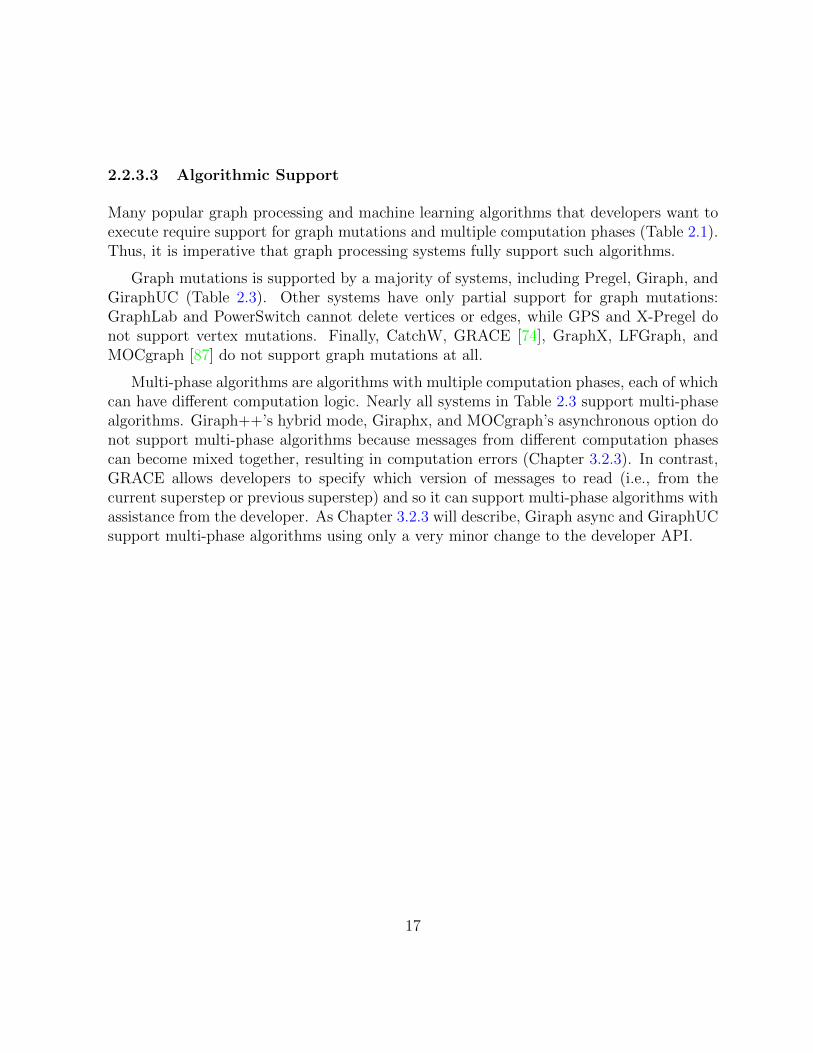
Many popular graph processing and machine learning algorithms that developers want toexecute require support for graph mutations and multiple computation phases (Table 2.1).Thus, it is imperative that graph processing systems fully support such algorithms.
Graph mutations is supported by a majority of systems, including Pregel, Giraph, andGiraphUC (Table 2.3). Other systems have only partial support for graph mutations:GraphLab and PowerSwitch cannot delete vertices or edges, while GPS and X-Pregel donot support vertex mutations. Finally, CatchW, GRACE [74], GraphX, LFGraph, andMOCgraph [87] do not support graph mutations at all.
Multi-phase algorithms are algorithms with multiple computation phases, each of whichcan have different computation logic. Nearly all systems in Table 2.3 support multi-phasealgorithms. Giraph++’s hybrid mode, Giraphx, and MOCgraph’s asynchronous option donot support multi-phase algorithms because messages from different computation phasescan become mixed together, resulting in computation errors (Chapter 3.2.3). In contrast,GRACE allows developers to specify which version of messages to read (i.e., from thecurrent superstep or previous superstep) and so it can support multi-phase algorithms withassistance from the developer. As Chapter 3.2.3 will describe, Giraph async and GiraphUCsupport multi-phase algorithms using only a very minor change to the developer API.
17
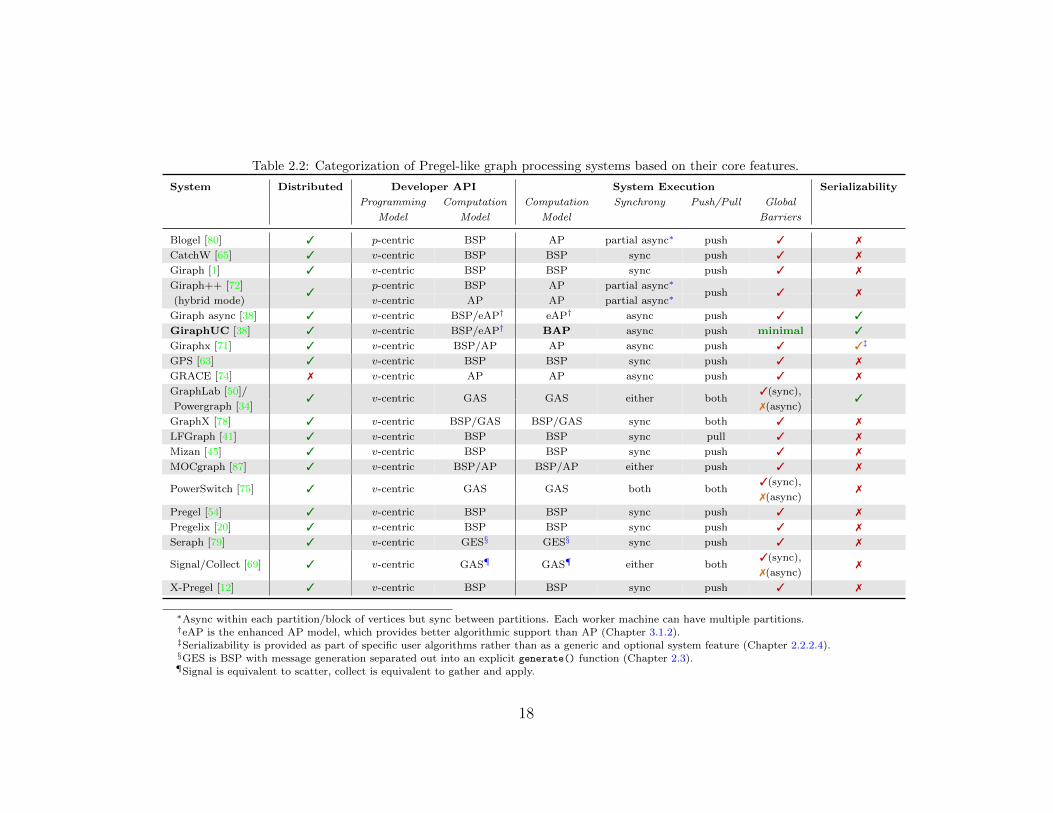
Table 2.2: Categorization of Pregel-like graph processing systems based on their core features.
System Distributed Developer API System Execution Serializability
Programming Computation Computation Synchrony Push/Pull Global
Model Model Model Barriers
Blogel [80] 3 p-centric BSP AP partial async∗ push 3 7
CatchW [65] 3 v-centric BSP BSP sync push 3 7
Giraph [1] 3 v-centric BSP BSP sync push 3 7
Giraph++ [72] p-centric BSP AP partial async∗
(hybrid mode)3
v-centric AP AP partial async∗push 3 7
Giraph async [38] 3 v-centric BSP/eAP† eAP† async push 3 3
GiraphUC [38] 3 v-centric BSP/eAP† BAP async push minimal 3
Giraphx [71] 3 v-centric BSP/AP AP async push 3 3‡
GPS [63] 3 v-centric BSP BSP sync push 3 7
GRACE [74] 7 v-centric AP AP async push 3 7
GraphLab [50]/ 3(sync),
Powergraph [34]3 v-centric GAS GAS either both
7(async)3
GraphX [78] 3 v-centric BSP/GAS BSP/GAS sync both 3 7
LFGraph [41] 3 v-centric BSP BSP sync pull 3 7
Mizan [45] 3 v-centric BSP BSP sync push 3 7
MOCgraph [87] 3 v-centric BSP/AP BSP/AP either push 3 7
3(sync),PowerSwitch [75] 3 v-centric GAS GAS both both
7(async)7
Pregel [54] 3 v-centric BSP BSP sync push 3 7
Pregelix [20] 3 v-centric BSP BSP sync push 3 7
Seraph [79] 3 v-centric GES§ GES§ sync push 3 7
3(sync),Signal/Collect [69] 3 v-centric GAS¶ GAS¶ either both
7(async)7
X-Pregel [12] 3 v-centric BSP BSP sync push 3 7
∗Async within each partition/block of vertices but sync between partitions. Each worker machine can have multiple partitions.†eAP is the enhanced AP model, which provides better algorithmic support than AP (Chapter 3.1.2).‡Serializability is provided as part of specific user algorithms rather than as a generic and optional system feature (Chapter 2.2.2.4).§GES is BSP with message generation separated out into an explicit generate() function (Chapter 2.3).¶Signal is equivalent to scatter, collect is equivalent to gather and apply.
18
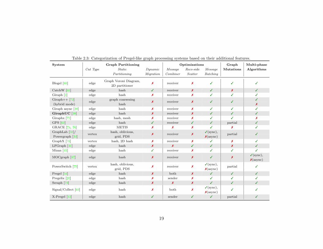
Table 2.3: Categorization of Pregel-like graph processing systems based on their additional features.
System Graph Partitioning Optimizations Graph Multi-phase
Cut Type Static Dynamic Message Recv-side Message Mutations Algorithms
Partitioning Migration Combiner Scatter Batching
Graph Voroni Diagram,Blogel [80] edge
2D partitioner7 receiver 7 3 3 3
CatchW [65] edge hash 3 receiver 7 3 7 3
Giraph [1] edge hash 7 receiver 7 3 3 3
Giraph++ [72] graph coarsening 3
(hybrid mode)edge
hash7 receiver 7 3 3
7
Giraph async [38] edge hash 7 receiver 7 3 3 3
GiraphUC [38] edge hash 7 receiver 7 3 3 3
Giraphx [71] edge hash, mesh 7 receiver 7 3 3 7
GPS [63] edge hash 3 receiver 3 3 partial 3
GRACE [74, 76] edge METIS 7 7 7 3 7 3
GraphLab [50]/ hash, oblivious, 3(sync),
Powergraph [34]vertex
grid, PDS7 receiver 7
7(async)partial 3
GraphX [78] vertex hash, 2D hash 7 receiver 7 3 7 3
LFGraph [41] edge hash 7 7 3 3 7 3
Mizan [45] edge hash 3 receiver 7 3 3 3
3(sync),MOCgraph [87] edge hash 7 receiver 7 3 7
7(async)
hash, oblivious, 3(sync),PowerSwitch [75] vertex
grid, PDS7 receiver 7
7(async)partial 3
Pregel [54] edge hash 7 both 7 3 3 3
Pregelix [20] edge hash 7 sender 7 3 3 3
Seraph [79] edge hash 7 7 7 3 3 3
3(sync),Signal/Collect [69] edge hash 7 both 7
7(async)3 3
X-Pregel [12] edge hash 3 sender 3 3 partial 3
19
2.3 Pregel-like Graph Processing Systems
We now provide some additional details for a subset of the Pregel-like systems describedin Chapter 2.2 and categorized in Tables 2.2 and 2.3.
CatchW is built on top of Apache Hama [3], which is a general BSP system that is notoptimized for graph processing and does not support graph mutations. As described inChapter 2.2.3.1, CatchW and Mizan are systems that focus on more sophisticated dynamicmigration schemes, whereas GPS and X-Pregel offer simpler and more lightweight schemes.X-Pregel [12] is an implementation of Pregel using IBM’s X10 programming language.
Giraph++ [72] primarily focuses on a graph-centric programming model but also con-siders a separate vertex-centric hybrid mode that implements a partially async AP model(Chapter 2.2.2). GRACE [74] is a single-machine shared memory system that is not dis-tributed and does not support disk-based computation. GRACE implements the AP modelthrough user customizable vertex scheduling and message selection, which can complicatethe developer API. In contrast, GiraphUC preserves Giraph’s simple BSP developer in-terface. GRACE also requires an immutable graph structure and so it does not supportgraph mutations.
GraphX [78] is built on the data parallel engine Spark [82] and presents a ResilientDistributed Graph (RDG) programming abstraction in which graphs are stored as tabulardata and graph operations are implemented using distributed joins. GraphX supports bothBSP and sync GAS (but not async GAS) and its primary goal is to provide more efficientgraph processing for end-to-end data analytic pipelines implemented in Spark. Similarly,Pregelix [20] implements BSP graph processing in Hyracks [18], a shared-nothing dataflowengine, and stores graphs and messages as data tuples and uses joins to implement messagepassing.
The design of LFGraph [41] is based on the notion that hash partitioning is sufficientfor static graph partitioning and that combiners are unnecessary. It is unique in that it isa pull-based BSP system where vertices store only their in-edges. In contrast, nearly allother BSP systems are push-based and have vertices store their out-edges.
MOCgraph [87] is a system that provides a combiner optimization, called message onlinecomputing (MOC), which immediately applies received messages to the recipient’s vertexvalue instead of buffering them in a message store and applying them when the vertexis next executed. Similar to message combiners (Chapter 2.2.3.2), the combine operationis specified by a user-defined onlineCompute() function that must be commutative andassociative. MOCgraph also considers an optimization for out-of-core (disk-based) com-putation, where each machine exchanges vertices between its own partitions such that hot
20
vertices are co-located on the same partitions. Machines can then keep these hot parti-tions in-memory and, instead of frequently loading cold partitions into memory (which iscostly), dump messages for cold partitions directly to disk and only occasionally load coldpartitions into memory to apply these messages.
Seraph [79] is a vertex-centric BSP system that allows multiple algorithms to executeon a shared input graph. This is in contrast to existing systems, where executing multiplealgorithms requires each algorithm to store its own copy of the input graph in memory, assuch systems focus on executing only one algorithm at a time. Seraph’s approach allowsthe input graph to be shared, which considerably lowers the memory costs of algorithmsoperating on the same input graph. It introduces a new GES model, where developersplace message generation code inside a generate() function rather than in the per-vertexcompute function. The GES model is otherwise identical to BSP.
Lastly, Signal/Collect [69] was one of the first systems to consider an explicit two-phasegather-scatter approach. This is different from systems like Pregel and Giraph, whichhave an explicit scatter (send) but implicit gather (receive). The scatter-gather model isessentially identical to GraphLab’s GAS model, only with gather and apply occurring asa single phase.
2.4 Other Related Systems
Finally, there are several other systems related to graph processing but deviate from ourcore focus on specialized in-memory Pregel-like graph processing systems. These additionalsystems can be broadly categorized as iterative MapReduce systems, graph databases,single-machine disk-based systems, or Pregel-like graph processing on generic big datasystems.
MapReduce [29] is an early programming model introduced for performing large-scaledistributed data computations. However, it does not natively support iterative computa-tion, which is required by graph processing. Consequently, performing graph processingon MapReduce incurs significant performance penalties: the input graph is shuffled be-tween mappers and reducers on every iteration, which adds substantial communicationoverheads. Furthermore, the graph is written to disk at the end of each MapReduce iter-ation and streamed back into memory for the next iteration, resulting in unnecessary andcostly disk I/O. HaLoop [21], iMapReduce [83], PrIter [84], Stratophere [10], Surfer [23],and Twister [31] are all systems developed to both reduce these performance overheadsand improve the developer interface for iterative MapReduce. While these systems outper-form regular MapReduce systems like Hadoop [2], their performance on graph processing
21
tasks remains worse than specialized Pregel-like graph processing systems. For example,Stratosphere is up to two times slower than Giraph 0.2 [10], a version of Giraph that isover two years older than the current and substantially more performant Giraph 1.1.0 [1].
Graph databases are systems that persistently store databases in the format of a graph.In contrast to iterative MapReduce and Pregel-like systems, graph databases focus on pro-viding persistence graph storage and support for online queries on the stored graph. Con-sequently, existing graph databases have either little or no support for the sophisticatedoffline graph analytics possible in specialized Pregel-like systems. For example, the populargraph database Titan [7] features a graph analytics engine Faunus [61], which uses MapRe-duce instead of a Pregel-like approach. Other popular graph databases include OrientDB[6] and Neo4j [4].
In addition to distributed in-memory Pregel-like systems, there are currently two otherimportant avenues that researchers are investigating.
The first is single-machine disk-based Pregel-like systems, which spill large input graphsout to disk. GraphChi [48] was one of the first vertex-centric systems to consider this ap-proach and introduced a parallel sliding windows technique to minimize non-sequential diskI/O. X-Stream [62], in contrast, uses an edge-centric programming model (Chapter 2.2.1)to avoid random I/O. TurboGraph [40] further improves on GraphChi by using techniquesthat exploit the I/O parallelism of SSDs. More recent systems include FlashGraph [86],which considers techniques for arrays of SSDs, and VENUS [24], which introduces a moreefficient model of storing and accessing graph data on disk as well as caching strategies tofurther improve performance.
The second avenue is supporting Pregel-like graph processing on more generic big datasystems, such as relational databases. This direction is motivated by the need for betterintegration with existing big data tools, as well as the fact that a large portion of the datathat developers want to analyze are already stored in a relational format: using specializedPregel-like systems would first require converting this data into a suitable graph formatbefore analytics can occur. As described in Chapter 2.3, GraphX [78] and Pregelix [20] aredesigned with this in mind: they both store graphs as tabular data, which easily integrateswith the tabular format used by the other tools of the data engines on which they arebuilt. Consequently, they are more generic than, for example, Giraph and GraphLab.Similarly, Trinity [66] uses a globally addressable in-memory key-value store, where data ispartitioned across workers by their keys rather than by vertex or edge IDs, and it supportsboth online queries and offline graph analytics. Aster Graph Analytics [68], GRAIL [32],and Vertexica [42] address Pregel-like graph processing on relational databases by mappinga subset of graph analytic tasks to relational operations.
22
Chapter 3
Giraph Unchained: BarrierlessAsynchronous Parallel Execution
We begin this chapter by motivating BAP through a detailed discussion of the shortcomingsof the BSP, AP, and GAS models. We then introduce our BAP model and its implemen-tation, GiraphUC, in Chapters 3.2 and 3.3. We provide an experimental evaluation inChapter 3.4 and conclude with a summary in Chapter 3.5.
3.1 Motivation
3.1.1 Performance
In BSP, global barriers ensure that all messages sent in one superstep are delivered be-fore the start of the next superstep, thus resolving implicit data dependencies encoded inmessages. However, the synchronous execution enforced by these global barriers causesBSP to suffer from major performance limitations: stale messages, large communicationoverheads, and high synchronization costs due to stragglers.
To illustrate these limitations concretely, Figures 3.1a and 3.1b visualize the BSP andAP executions of our WCC example (Chapter 2.1) with explicit global barriers and withtime flowing horizontally from left to right. The green regions indicate computation whilethe red striped and gray regions indicate that a worker is blocked on communication oron a barrier, respectively. For simplicity, assume that the communication overheads andglobal barrier processing times are constant.
23
Running: Blocked (comm.): Blocked (barrier):
W1
W2
W3
Global barrier
(a) BSP
W1
W2
W3
(b) AP
W1
W2
W3
Local barrier
(c) BAP
Figure 3.1: Computation times for the WCC example under different computation models.
Stale messages. As described in Chapter 2.1.2, reducing stale messages allows theAP execution of WCC to finish in fewer supersteps than the BSP execution, translating toshorter computation time. In general, allowing vertices to see more recent (less stale) datato update their per-vertex parameters enables faster convergence and shorter computationtimes, resulting in better performance [50]. Our proposed BAP model preserves theseadvantages of the AP model by also reducing message staleness without using distributedlocking (Chapter 3.2).
Communication overheads. Since BSP and AP execute only one superstep betweenglobal barriers, there is usually insufficient computation work to adequately overlap withand mask communication overheads. For example, in Figures 3.1a and 3.1b, workersspend a large portion of their time blocked on communication. Furthermore, for AP, thecommunication overheads can outweigh performance gains achieved by reducing messagestaleness. Figure 3.1c illustrates how our proposed BAP model resolves this by minimizingthe use of global barriers: each worker can perform multiple logical supersteps (separatedby inexpensive local barriers) without global barriers (Chapter 3.2), which greatly improvesthe overlap between computation and communication.
Stragglers and synchronization costs. Stragglers are the slowest workers in acomputation. They are caused by a variety of factors, some as simple as unbalancedhardware resources and others that are more complex. For example, the power-law degreedistribution of natural graphs used in computations can result in substantial computationand communication load for a handful of workers due to the extremely high degrees of a
24
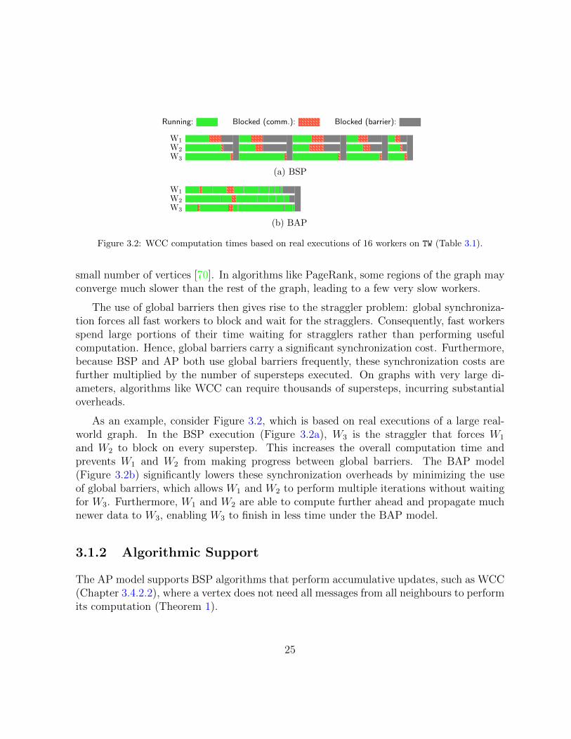
Running: Blocked (comm.): Blocked (barrier):
W1
W2
W3
(a) BSP
W1
W2
W3
(b) BAP
Figure 3.2: WCC computation times based on real executions of 16 workers on TW (Table 3.1).
small number of vertices [70]. In algorithms like PageRank, some regions of the graph mayconverge much slower than the rest of the graph, leading to a few very slow workers.
The use of global barriers then gives rise to the straggler problem: global synchroniza-tion forces all fast workers to block and wait for the stragglers. Consequently, fast workersspend large portions of their time waiting for stragglers rather than performing usefulcomputation. Hence, global barriers carry a significant synchronization cost. Furthermore,because BSP and AP both use global barriers frequently, these synchronization costs arefurther multiplied by the number of supersteps executed. On graphs with very large di-ameters, algorithms like WCC can require thousands of supersteps, incurring substantialoverheads.
As an example, consider Figure 3.2, which is based on real executions of a large real-world graph. In the BSP execution (Figure 3.2a), W3 is the straggler that forces W1
and W2 to block on every superstep. This increases the overall computation time andprevents W1 and W2 from making progress between global barriers. The BAP model(Figure 3.2b) significantly lowers these synchronization overheads by minimizing the useof global barriers, which allows W1 and W2 to perform multiple iterations without waitingfor W3. Furthermore, W1 and W2 are able to compute further ahead and propagate muchnewer data to W3, enabling W3 to finish in less time under the BAP model.
3.1.2 Algorithmic Support
The AP model supports BSP algorithms that perform accumulative updates, such as WCC(Chapter 3.4.2.2), where a vertex does not need all messages from all neighbours to performits computation (Theorem 1).
25
W1 W1 W1 W1
W2 W2
W3 W3 W3
W1
W2
W3
Global BarrierLocal Barrier
LSS 1 LSS 2 LSS 3 LSS 4
LSS 1 LSS 2
LSS 1 LSS 2 LSS 3
GSS 1 GSS 2
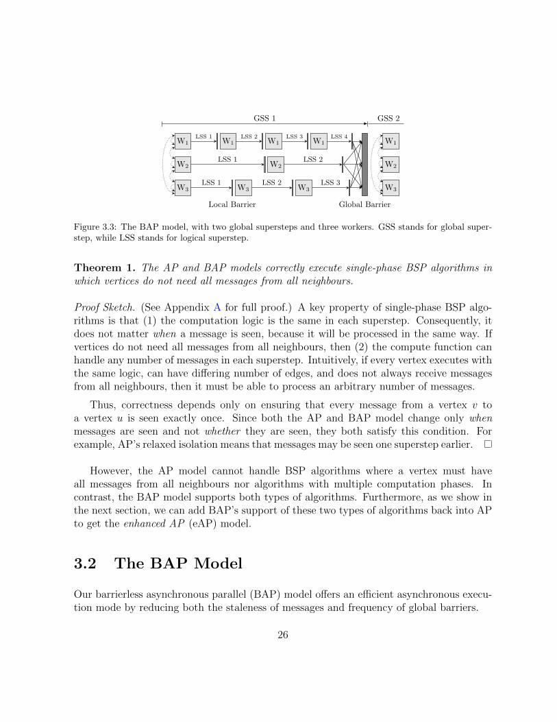
Figure 3.3: The BAP model, with two global supersteps and three workers. GSS stands for global super-step, while LSS stands for logical superstep.
Theorem 1. The AP and BAP models correctly execute single-phase BSP algorithms inwhich vertices do not need all messages from all neighbours.
Proof Sketch. (See Appendix A for full proof.) A key property of single-phase BSP algo-rithms is that (1) the computation logic is the same in each superstep. Consequently, itdoes not matter when a message is seen, because it will be processed in the same way. Ifvertices do not need all messages from all neighbours, then (2) the compute function canhandle any number of messages in each superstep. Intuitively, if every vertex executes withthe same logic, can have differing number of edges, and does not always receive messagesfrom all neighbours, then it must be able to process an arbitrary number of messages.
Thus, correctness depends only on ensuring that every message from a vertex v toa vertex u is seen exactly once. Since both the AP and BAP model change only whenmessages are seen and not whether they are seen, they both satisfy this condition. Forexample, AP’s relaxed isolation means that messages may be seen one superstep earlier.
However, the AP model cannot handle BSP algorithms where a vertex must haveall messages from all neighbours nor algorithms with multiple computation phases. Incontrast, the BAP model supports both types of algorithms. Furthermore, as we show inthe next section, we can add BAP’s support of these two types of algorithms back into APto get the enhanced AP (eAP) model.
3.2 The BAP Model
Our barrierless asynchronous parallel (BAP) model offers an efficient asynchronous execu-tion mode by reducing both the staleness of messages and frequency of global barriers.
26
As discussed in Chapter 3.1.1, global barriers limit performance in both the BSP andAP models. The BAP model avoids global barriers by using local barriers that separatelogical supersteps. Unlike global barriers, local barriers do not require global coordination:they are local to each worker and are used only as a pausing point to perform tasks likegraph mutations and to decide whether a global barrier is necessary. Since local barriersare internal to the system, they occur automatically and are transparent to developers.
A logical superstep is logically equivalent to a regular BSP superstep in that bothexecute vertices exactly once and are numbered with strictly increasing values. However,unlike BSP supersteps, logical supersteps are not globally coordinated and so differentworkers can execute a different number of logical supersteps. We use the term globalsupersteps to refer to collections of logical supersteps that are separated by global barriers.Figure 3.3 illustrates two global supersteps (GSS 1 and GSS 2) separated by a globalbarrier. In the first global superstep, worker 1 executes four logical supersteps, whileworkers 2 and 3 execute two and three logical supersteps respectively. In contrast, BSPand AP have exactly one logical superstep per global superstep.
Local barriers and logical supersteps enable fast workers to continue execution insteadof blocking, which minimizes communication and synchronization overheads and mitigatesthe straggler problem (Chapter 3.1.1). Logical supersteps are thus much cheaper than BSPsupersteps as they avoid synchronization costs. Local barriers are also much faster than theprocessing times of global barriers alone (i.e., excluding synchronization costs), since theydo not require global communication. Hence, per-superstep overheads are substantiallysmaller in the BAP model, which results in significantly better performance.
Finally, as in the AP model, the BAP model reduces message staleness by allowingvertices to immediately see local and remote messages that they have received. In Fig-ure 3.3, dotted arrows represent messages received and seen/processed in the same logicalsuperstep, while solid arrows indicate messages that are not processed until the next logicalsuperstep. For clarity, we omit dotted arrows between every worker box but note that theydo exist.
Next, we present details about local barriers and algorithmic support in the BAP model.
3.2.1 Local Barriers
For simplicity, we first focus on algorithms with a single computation phase. Algorithmswith multiple computation phases are discussed in Chapter 3.2.3.
27
LSS i Msgs? LSS i + 1
GB
Yes
No
(a) Naive approach.
LSS i Msgs?
Lightweight GB
LSS i + 1
GB
Yes
No
Receive msg All workersarrive
(b) Improved approach.
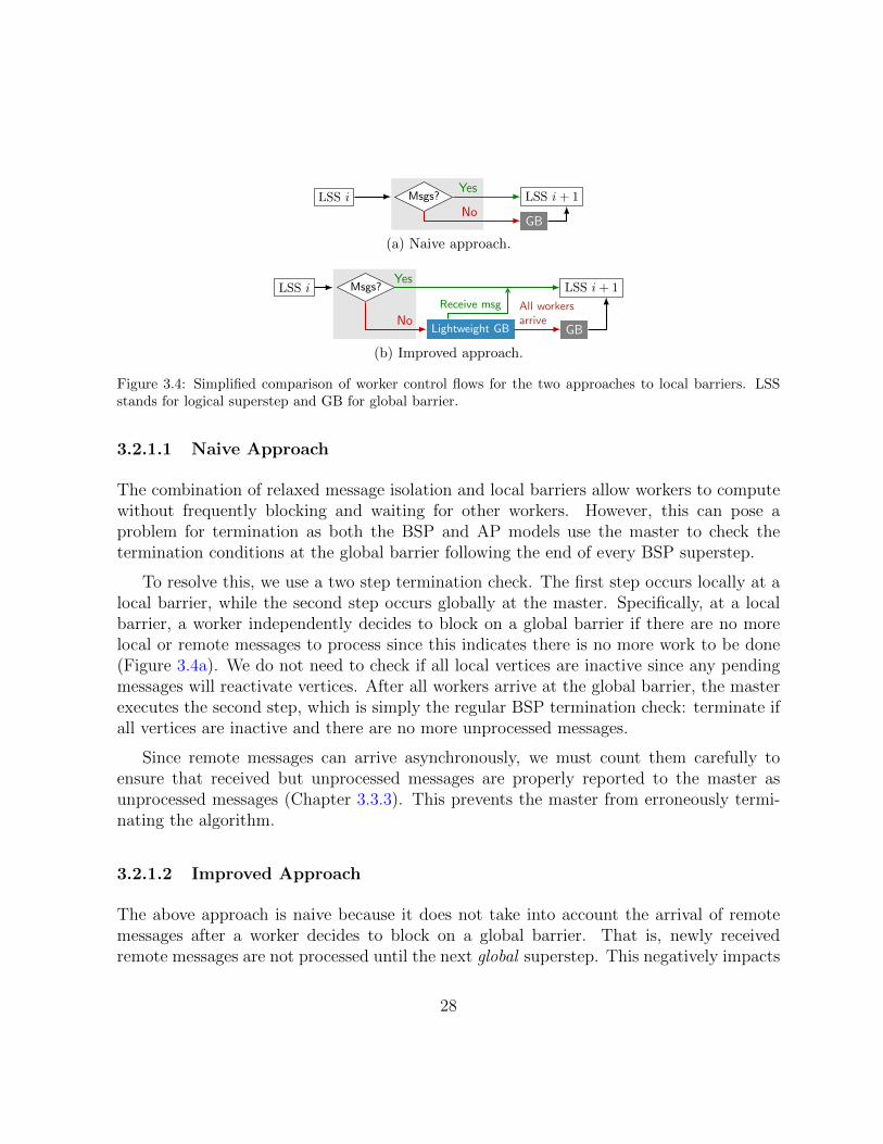
Figure 3.4: Simplified comparison of worker control flows for the two approaches to local barriers. LSSstands for logical superstep and GB for global barrier.
3.2.1.1 Naive Approach
The combination of relaxed message isolation and local barriers allow workers to computewithout frequently blocking and waiting for other workers. However, this can pose aproblem for termination as both the BSP and AP models use the master to check thetermination conditions at the global barrier following the end of every BSP superstep.
To resolve this, we use a two step termination check. The first step occurs locally at alocal barrier, while the second step occurs globally at the master. Specifically, at a localbarrier, a worker independently decides to block on a global barrier if there are no morelocal or remote messages to process since this indicates there is no more work to be done(Figure 3.4a). We do not need to check if all local vertices are inactive since any pendingmessages will reactivate vertices. After all workers arrive at the global barrier, the masterexecutes the second step, which is simply the regular BSP termination check: terminate ifall vertices are inactive and there are no more unprocessed messages.
Since remote messages can arrive asynchronously, we must count them carefully toensure that received but unprocessed messages are properly reported to the master asunprocessed messages (Chapter 3.3.3). This prevents the master from erroneously termi-nating the algorithm.
3.2.1.2 Improved Approach
The above approach is naive because it does not take into account the arrival of remotemessages after a worker decides to block on a global barrier. That is, newly receivedremote messages are not processed until the next global superstep. This negatively impacts
28
Running: Blocked (comm.): Blocked (barrier):
W1
W2
W3
Global barrier Local barrier
(a) Naive approach: workers remain blocked.
W1
W2
W3
Unblock to process new messages
(b) Improved approach: workers unblock to process new mes-sages. Blue regions indicate lightweight global barrier.
Figure 3.5: Performance comparison between the naive vs. improved approach, based on SSSP executionsof 16 workers on TW (Table 3.1).
performance as workers can remain blocked for a long time, especially in the presence ofstragglers, and it also results in more frequent global barriers since the inability to unblockfrom a barrier means that all workers eventually stop generating messages.
For example, the single source shortest path (SSSP) algorithm begins with only oneactive vertex (the source), so the number of messages sent between vertices increases, peaksand then decreases with time (Chapter 3.4.2.1). Figure 3.5a shows an SSSP execution usingthe naive approach, where W1 and W3 initially block on a global barrier as they have littlework to do. Even if messages from W2 arrive, W1 and W3 will remain blocked. In thesecond global superstep, W2 remains blocked for a very long time due to W1 and W3 beingable to execute many logical supersteps before running out of work to do. As a result, alarge portion of time is spent blocked on global barriers.
However, if we allow workers to unblock and process new messages with additionallogical supersteps, we can greatly reduce the unnecessary blocking and shorten the totalcomputation time (Figure 3.5b). The improved approach does precisely this: we inserta lightweight global barrier, before the existing (BSP) global barrier, that allows workersto unblock upon receiving a new message (Figure 3.4b). This additional global barrier islightweight because it is cheaper to block and unblock from compared to the (BSP) globalbarrier (Chapter 3.3.3). Unblocking under the above condition is also efficient becausemessages arrive in batches (Chapter 3.3.2), so there is always sufficient new work to do.
Additionally, with this improved approach, if each worker Wi waits for all its sentmessages to be delivered (acknowledged) before blocking, the recipient workers will unblockbefore Wi can block. This means that all workers arrive at the lightweight global barrier
29
(and proceed to the (BSP) global barrier) only when there are no messages among anyworkers. This allows algorithms with a single computation phase to be completed in exactlyone global superstep.
Hence, local barriers ensure that algorithms are executed using the minimal number ofglobal supersteps, which minimizes communication and synchronization overheads. Fur-thermore, the two step termination check is more efficient and scalable than the distributedconsensus algorithm used by GraphLab async, as our experimental results will show (Chap-ter 3.4.3). Finally, unlike GraphLab and its GAS model, BAP fully supports graph muta-tions by having workers resolve pending mutations during a local barrier (Chapter 3.3.4).
3.2.2 Algorithmic Support
The BAP model, like the AP model, supports single-phase algorithms that do not needall messages from all neighbours (Theorem 1). Theorem 2 shows how the BAP modelalso supports algorithms where vertices do require all messages from all neighbours. Thistheorem also improves the algorithmic support of the AP model, to give the eAP model.
Theorem 2. Given a message store that is initially filled with valid messages, retains oldmessages, and overwrites old messages with new messages, the BAP model correctly exe-cutes single-phase BSP algorithms in which vertices need all messages from all neighbours.
Proof Sketch. (See Appendix A for full proof.) Like in Theorem 1’s proof sketch, weagain have property (1), so when a message is seen is unimportant. Since vertices need allmessages from all (in-edge) neighbours, we also have that (2) an old message m from vertexv to u can be overwritten by a new message m′ from v to u. The intuition is that sinceevery vertex needs messages from all its in-edge neighbours, it must also send a messageto each of its out-edge neighbours. This means a newer message contains a more recentstate of a neighbour, which can safely overwrite the old message that now contains a stalestate.
Correctness requires that every vertex u sees exactly one message from each of itsin-edge neighbours in each (logical) superstep. That is, u must see exactly N = deg−(u)messages. The message store described in the theorem ensures that each u starts with, and(by retaining old messages) will always have, exactly N messages. Property (2) allows newincoming messages to overwrite corresponding old messages, again ensuring N messages.Thus, independent of the (logical) superstep of execution, u always sees N messages, soboth the AP and BAP models guarantee correctness.
30
Per Theorem 2, the message store must be initially filled with messages. This is achievedin the BAP model by adding a global barrier after the very first logical superstep of thealgorithm, when messages are sent for the first time.
3.2.3 Multiple Computation Phases
Algorithms with multiple computation phases are computations composed of multipletasks, where each task has different compute logic. Therefore, computation phases requireglobal coordination for correctness. To do so otherwise requires rewriting the algorithmsuch that it can no longer be programmed for BSP, which negatively impacts usability.
For example, in DMST (Chapter 3.4.2.3), the phase where vertices find a minimumweight out-edge occurs after the phase in which vertices add and remove edges. If thesetwo phases are not separated by a global barrier, the results will be incorrect as somevertices will not have completed their mutations yet. Hence, the BAP model must useglobal barriers to separate different computation phases. However, we can continue to uselocal barriers and logical supersteps within each computation phase, which allows eachphase to complete in a single global superstep (Chapter 3.2.1.2).
In addition to computation phases that have multiple supersteps, many multi-phasealgorithms have single-superstep phases (phases that are only one BSP superstep). Theseare typically used to send messages to be processed in the next phase. Even with globalbarriers separating computation phases, relaxed message isolation will cause vertices to seethese messages in the incorrect phase. In other words, messages for different phases willbe incorrectly mixed together. We handle these heterogeneous messages by considering allthe possible scenarios, as proved in Theorem 3.
Theorem 3. If every message is tagged with a Boolean at the API level and two messagestores are maintained at the system level, then the BAP model supports BSP algorithmswith multiple computation phases.
Proof. Since the BAP model executes only algorithms written for the BSP model, it sufficesto consider multi-phase algorithms implemented for BSP. For such algorithms, there areonly three types of messages: (1) a message sent in the previous phase k−1 to be processedin the current phase k; (2) a message sent in phase k to be processed in this same phase k;and (3) a message sent in phase k to be processed in the next phase k+1. Other scenarios,in which a message is sent in phase m to be processed in phase n where (n − m) > 1,are not possible due to a property of BSP: any message sent in one superstep is visibleonly in the next superstep, so messages not processed in the next superstep are lost. If
31
(n−m) > 1, then phases n and m are more than one superstep apart and so n cannot seethe messages sent by m. Since BAP separates computation phases with global barriers, itinherits this property from the BSP model.
For the two message stores, we use one store (call it MSC) to hold messages for thecurrent phase and the other store (call it MSN) to hold messages for the next phase. Whena new computation phase occurs, the MSN of the previous phase becomes the MSC of thecurrent phase, while the new MSN becomes empty. We use a Boolean to indicate whethera message, sent in the current phase, is to be processed in the next computation phase.Since all messages are tagged with this Boolean, we can determine which store (MSC orMSN) to store received messages into.
Thus, all three scenarios are covered: if (1), the message was placed in MSN duringphase k − 1, which becomes MSC in phase k and so the message is made visible in thecorrect phase; if (2), the message is placed in MSC of phase k, which is immediately visiblein phase k; finally, if (3), the message is placed in MSN of phase k, which will become theMSC of phase k + 1.
Theorem 3 implicitly requires knowledge of when a new phase starts in order to knowwhen to make MSN the new MSC . In BAP, the start and end of computation phasescan be inferred locally by each worker since each phase completes in one global superstep.That is, the start of a phase is simply the start of a global superstep, while the end of aphase is determined by checking if any more local or remote messages are available for thecurrent phase. Messages for the next phase are ignored, as they cannot be processed yet.Hence, the BAP model detects phase transitions without modifications to the developerAPI.
Theorem 3 is also applicable to the AP model, thus enhancing it to also support multi-phase algorithms. However, unlike BAP, the eAP model is unable to infer the start andend of computation phases, so it requires an additional API call for algorithms to notifythe system of a computation phase change (Chapter 3.3.5.1).
Chapter 3.3.5 describes an implementation that provides message tagging without in-troducing network overheads. Hence, the BAP model efficiently supports multi-phasealgorithms while preserving the BSP developer interface.
3.3 GiraphUC
We now describe GiraphUC, our implementation of the BAP model in Giraph. We useGiraph because it is a popular and performant push-based distributed graph processing
32
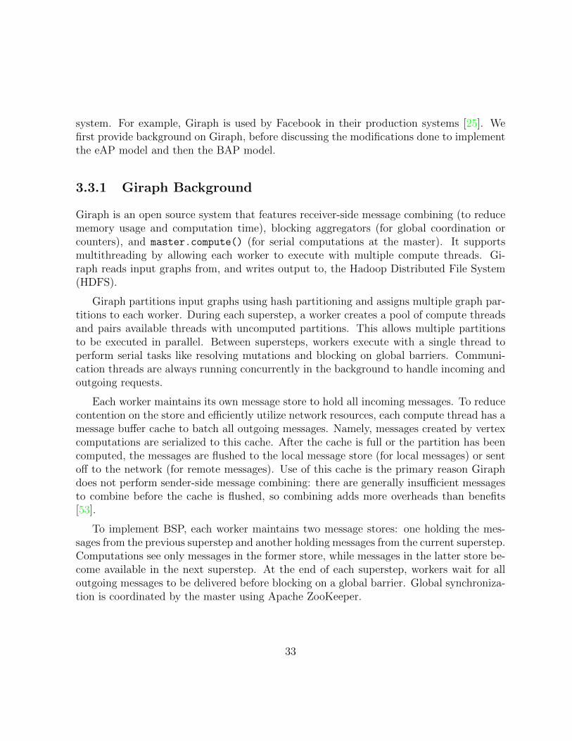
system. For example, Giraph is used by Facebook in their production systems [25]. Wefirst provide background on Giraph, before discussing the modifications done to implementthe eAP model and then the BAP model.
3.3.1 Giraph Background
Giraph is an open source system that features receiver-side message combining (to reducememory usage and computation time), blocking aggregators (for global coordination orcounters), and master.compute() (for serial computations at the master). It supportsmultithreading by allowing each worker to execute with multiple compute threads. Gi-raph reads input graphs from, and writes output to, the Hadoop Distributed File System(HDFS).
Giraph partitions input graphs using hash partitioning and assigns multiple graph par-titions to each worker. During each superstep, a worker creates a pool of compute threadsand pairs available threads with uncomputed partitions. This allows multiple partitionsto be executed in parallel. Between supersteps, workers execute with a single thread toperform serial tasks like resolving mutations and blocking on global barriers. Communi-cation threads are always running concurrently in the background to handle incoming andoutgoing requests.
Each worker maintains its own message store to hold all incoming messages. To reducecontention on the store and efficiently utilize network resources, each compute thread has amessage buffer cache to batch all outgoing messages. Namely, messages created by vertexcomputations are serialized to this cache. After the cache is full or the partition has beencomputed, the messages are flushed to the local message store (for local messages) or sentoff to the network (for remote messages). Use of this cache is the primary reason Giraphdoes not perform sender-side message combining: there are generally insufficient messagesto combine before the cache is flushed, so combining adds more overheads than benefits[53].
To implement BSP, each worker maintains two message stores: one holding the mes-sages from the previous superstep and another holding messages from the current superstep.Computations see only messages in the former store, while messages in the latter store be-come available in the next superstep. At the end of each superstep, workers wait for alloutgoing messages to be delivered before blocking on a global barrier. Global synchroniza-tion is coordinated by the master using Apache ZooKeeper.
33
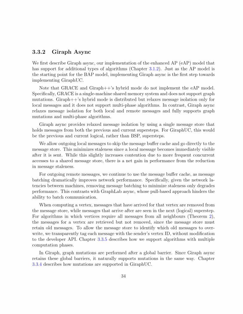
3.3.2 Giraph Async
We first describe Giraph async, our implementation of the enhanced AP (eAP) model thathas support for additional types of algorithms (Chapter 3.1.2). Just as the AP model isthe starting point for the BAP model, implementing Giraph async is the first step towardsimplementing GiraphUC.
Note that GRACE and Giraph++’s hybrid mode do not implement the eAP model.Specifically, GRACE is a single-machine shared memory system and does not support graphmutations. Giraph++’s hybrid mode is distributed but relaxes message isolation only forlocal messages and it does not support multi-phase algorithms. In contrast, Giraph asyncrelaxes message isolation for both local and remote messages and fully supports graphmutations and multi-phase algorithms.
Giraph async provides relaxed message isolation by using a single message store thatholds messages from both the previous and current supersteps. For GiraphUC, this wouldbe the previous and current logical, rather than BSP, supersteps.
We allow outgoing local messages to skip the message buffer cache and go directly to themessage store. This minimizes staleness since a local message becomes immediately visibleafter it is sent. While this slightly increases contention due to more frequent concurrentaccesses to a shared message store, there is a net gain in performance from the reductionin message staleness.
For outgoing remote messages, we continue to use the message buffer cache, as messagebatching dramatically improves network performance. Specifically, given the network la-tencies between machines, removing message batching to minimize staleness only degradesperformance. This contrasts with GraphLab async, whose pull-based approach hinders theability to batch communication.
When computing a vertex, messages that have arrived for that vertex are removed fromthe message store, while messages that arrive after are seen in the next (logical) superstep.For algorithms in which vertices require all messages from all neighbours (Theorem 2),the messages for a vertex are retrieved but not removed, since the message store mustretain old messages. To allow the message store to identify which old messages to over-write, we transparently tag each message with the sender’s vertex ID, without modificationto the developer API. Chapter 3.3.5 describes how we support algorithms with multiplecomputation phases.
In Giraph, graph mutations are performed after a global barrier. Since Giraph asyncretains these global barriers, it naturally supports mutations in the same way. Chapter3.3.4 describes how mutations are supported in GiraphUC.
34
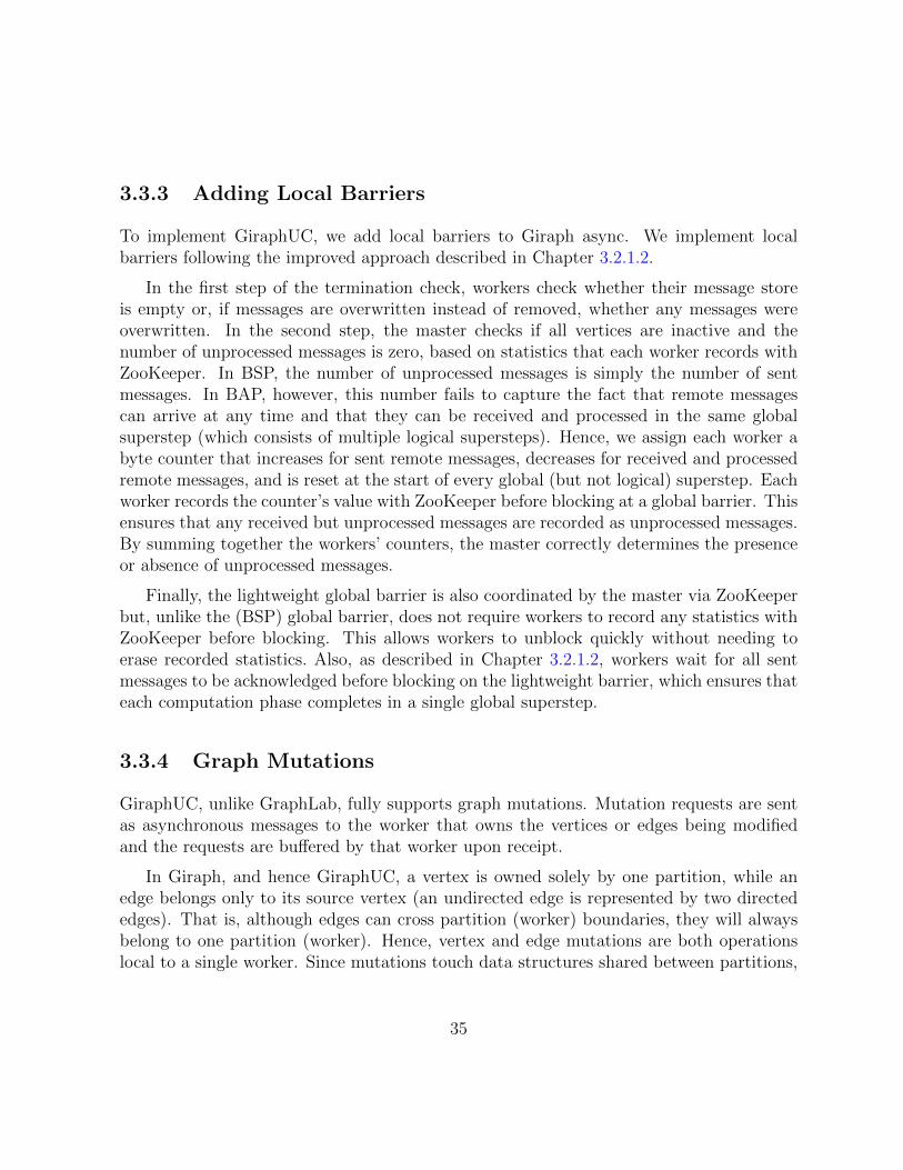
3.3.3 Adding Local Barriers
To implement GiraphUC, we add local barriers to Giraph async. We implement localbarriers following the improved approach described in Chapter 3.2.1.2.
In the first step of the termination check, workers check whether their message storeis empty or, if messages are overwritten instead of removed, whether any messages wereoverwritten. In the second step, the master checks if all vertices are inactive and thenumber of unprocessed messages is zero, based on statistics that each worker records withZooKeeper. In BSP, the number of unprocessed messages is simply the number of sentmessages. In BAP, however, this number fails to capture the fact that remote messagescan arrive at any time and that they can be received and processed in the same globalsuperstep (which consists of multiple logical supersteps). Hence, we assign each worker abyte counter that increases for sent remote messages, decreases for received and processedremote messages, and is reset at the start of every global (but not logical) superstep. Eachworker records the counter’s value with ZooKeeper before blocking at a global barrier. Thisensures that any received but unprocessed messages are recorded as unprocessed messages.By summing together the workers’ counters, the master correctly determines the presenceor absence of unprocessed messages.
Finally, the lightweight global barrier is also coordinated by the master via ZooKeeperbut, unlike the (BSP) global barrier, does not require workers to record any statistics withZooKeeper before blocking. This allows workers to unblock quickly without needing toerase recorded statistics. Also, as described in Chapter 3.2.1.2, workers wait for all sentmessages to be acknowledged before blocking on the lightweight barrier, which ensures thateach computation phase completes in a single global superstep.
3.3.4 Graph Mutations
GiraphUC, unlike GraphLab, fully supports graph mutations. Mutation requests are sentas asynchronous messages to the worker that owns the vertices or edges being modifiedand the requests are buffered by that worker upon receipt.
In Giraph, and hence GiraphUC, a vertex is owned solely by one partition, while anedge belongs only to its source vertex (an undirected edge is represented by two directededges). That is, although edges can cross partition (worker) boundaries, they will alwaysbelong to one partition (worker). Hence, vertex and edge mutations are both operationslocal to a single worker. Since mutations touch data structures shared between partitions,
35
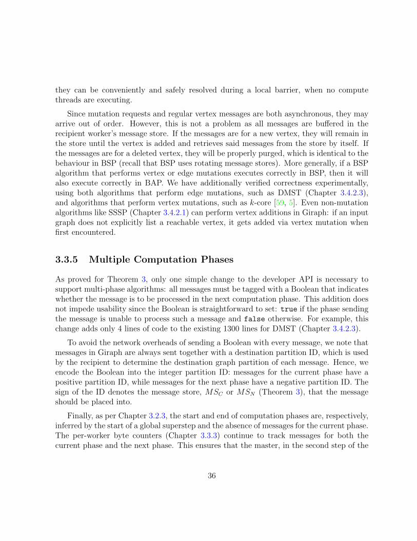
they can be conveniently and safely resolved during a local barrier, when no computethreads are executing.
Since mutation requests and regular vertex messages are both asynchronous, they mayarrive out of order. However, this is not a problem as all messages are buffered in therecipient worker’s message store. If the messages are for a new vertex, they will remain inthe store until the vertex is added and retrieves said messages from the store by itself. Ifthe messages are for a deleted vertex, they will be properly purged, which is identical to thebehaviour in BSP (recall that BSP uses rotating message stores). More generally, if a BSPalgorithm that performs vertex or edge mutations executes correctly in BSP, then it willalso execute correctly in BAP. We have additionally verified correctness experimentally,using both algorithms that perform edge mutations, such as DMST (Chapter 3.4.2.3),and algorithms that perform vertex mutations, such as k-core [59, 5]. Even non-mutationalgorithms like SSSP (Chapter 3.4.2.1) can perform vertex additions in Giraph: if an inputgraph does not explicitly list a reachable vertex, it gets added via vertex mutation whenfirst encountered.
3.3.5 Multiple Computation Phases
As proved for Theorem 3, only one simple change to the developer API is necessary tosupport multi-phase algorithms: all messages must be tagged with a Boolean that indicateswhether the message is to be processed in the next computation phase. This addition doesnot impede usability since the Boolean is straightforward to set: true if the phase sendingthe message is unable to process such a message and false otherwise. For example, thischange adds only 4 lines of code to the existing 1300 lines for DMST (Chapter 3.4.2.3).
To avoid the network overheads of sending a Boolean with every message, we note thatmessages in Giraph are always sent together with a destination partition ID, which is usedby the recipient to determine the destination graph partition of each message. Hence, weencode the Boolean into the integer partition ID: messages for the current phase have apositive partition ID, while messages for the next phase have a negative partition ID. Thesign of the ID denotes the message store, MSC or MSN (Theorem 3), that the messageshould be placed into.
Finally, as per Chapter 3.2.3, the start and end of computation phases are, respectively,inferred by the start of a global superstep and the absence of messages for the current phase.The per-worker byte counters (Chapter 3.3.3) continue to track messages for both thecurrent phase and the next phase. This ensures that the master, in the second step of the
36
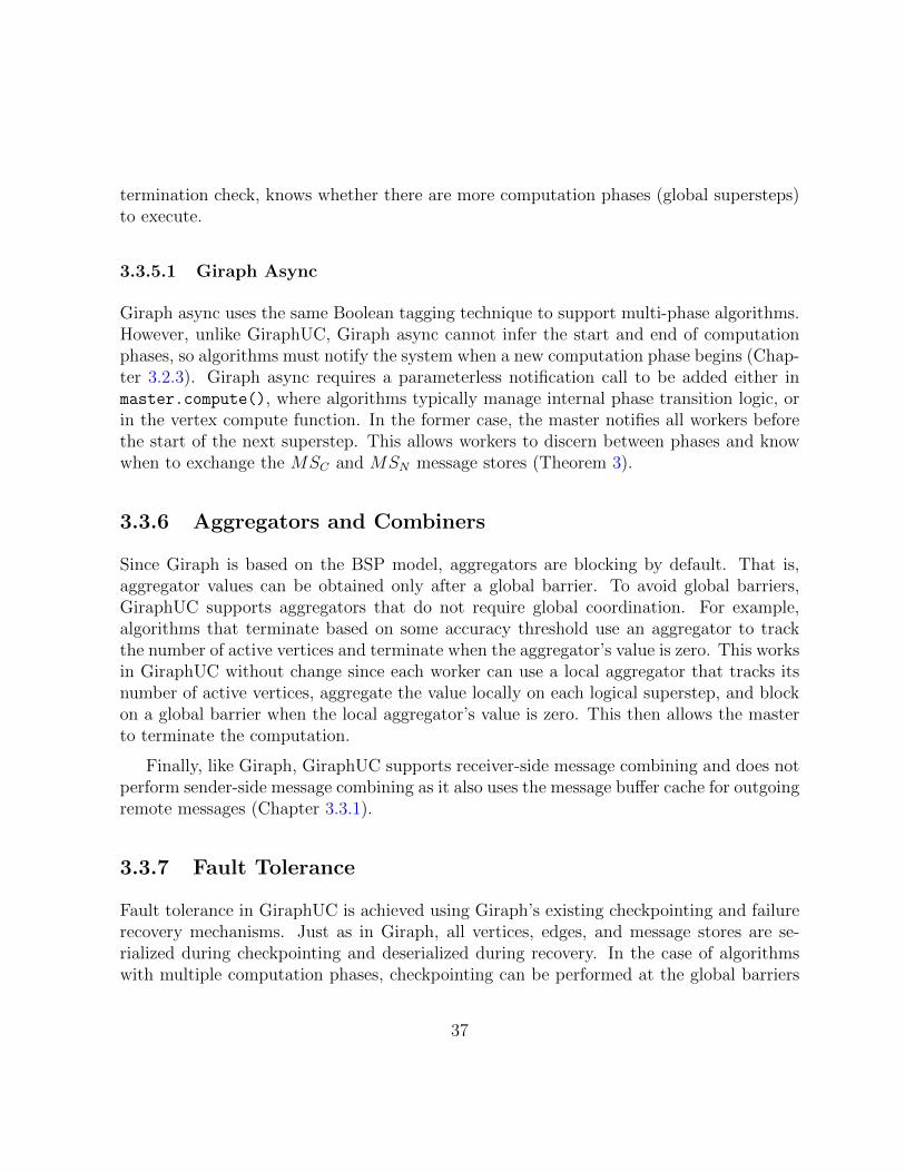
termination check, knows whether there are more computation phases (global supersteps)to execute.
3.3.5.1 Giraph Async
Giraph async uses the same Boolean tagging technique to support multi-phase algorithms.However, unlike GiraphUC, Giraph async cannot infer the start and end of computationphases, so algorithms must notify the system when a new computation phase begins (Chap-ter 3.2.3). Giraph async requires a parameterless notification call to be added either inmaster.compute(), where algorithms typically manage internal phase transition logic, orin the vertex compute function. In the former case, the master notifies all workers beforethe start of the next superstep. This allows workers to discern between phases and knowwhen to exchange the MSC and MSN message stores (Theorem 3).
3.3.6 Aggregators and Combiners
Since Giraph is based on the BSP model, aggregators are blocking by default. That is,aggregator values can be obtained only after a global barrier. To avoid global barriers,GiraphUC supports aggregators that do not require global coordination. For example,algorithms that terminate based on some accuracy threshold use an aggregator to trackthe number of active vertices and terminate when the aggregator’s value is zero. This worksin GiraphUC without change since each worker can use a local aggregator that tracks itsnumber of active vertices, aggregate the value locally on each logical superstep, and blockon a global barrier when the local aggregator’s value is zero. This then allows the masterto terminate the computation.
Finally, like Giraph, GiraphUC supports receiver-side message combining and does notperform sender-side message combining as it also uses the message buffer cache for outgoingremote messages (Chapter 3.3.1).
3.3.7 Fault Tolerance
Fault tolerance in GiraphUC is achieved using Giraph’s existing checkpointing and failurerecovery mechanisms. Just as in Giraph, all vertices, edges, and message stores are se-rialized during checkpointing and deserialized during recovery. In the case of algorithmswith multiple computation phases, checkpointing can be performed at the global barriers
37
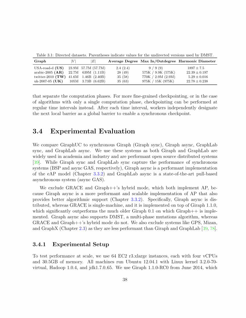
Table 3.1: Directed datasets. Parentheses indicate values for the undirected versions used by DMST.
Graph |V | |E| Average Degree Max In/Outdegree Harmonic Diameter
USA-road-d (US) 23.9M 57.7M (57.7M) 2.4 (2.4) 9 / 9 (9) 1897± 7.5arabic-2005 (AR) 22.7M 639M (1.11B) 28 (49) 575K / 9.9K (575K) 22.39± 0.197twitter-2010 (TW) 41.6M 1.46B (2.40B) 35 (58) 770K / 2.9M (2.9M) 5.29± 0.016uk-2007-05 (UK) 105M 3.73B (6.62B) 35 (63) 975K / 15K (975K) 22.78± 0.238
that separate the computation phases. For more fine-grained checkpointing, or in the caseof algorithms with only a single computation phase, checkpointing can be performed atregular time intervals instead. After each time interval, workers independently designatethe next local barrier as a global barrier to enable a synchronous checkpoint.
3.4 Experimental Evaluation
We compare GiraphUC to synchronous Giraph (Giraph sync), Giraph async, GraphLabsync, and GraphLab async. We use these systems as both Giraph and GraphLab arewidely used in academia and industry and are performant open source distributed systems[39]. While Giraph sync and GraphLab sync capture the performance of synchronoussystems (BSP and async GAS, respectively), Giraph async is a performant implementationof the eAP model (Chapter 3.3.2) and GraphLab async is a state-of-the-art pull-basedasynchronous system (async GAS).
We exclude GRACE and Giraph++’s hybrid mode, which both implement AP, be-cause Giraph async is a more performant and scalable implementation of AP that alsoprovides better algorithmic support (Chapter 3.3.2). Specifically, Giraph async is dis-tributed, whereas GRACE is single-machine, and it is implemented on top of Giraph 1.1.0,which significantly outperforms the much older Giraph 0.1 on which Giraph++ is imple-mented. Giraph async also supports DMST, a multi-phase mutations algorithm, whereasGRACE and Giraph++’s hybrid mode do not. We also exclude systems like GPS, Mizan,and GraphX (Chapter 2.3) as they are less performant than Giraph and GraphLab [39, 78].
3.4.1 Experimental Setup
To test performance at scale, we use 64 EC2 r3.xlarge instances, each with four vCPUsand 30.5GB of memory. All machines run Ubuntu 12.04.1 with Linux kernel 3.2.0-70-virtual, Hadoop 1.0.4, and jdk1.7.0 65. We use Giraph 1.1.0-RC0 from June 2014, which
38
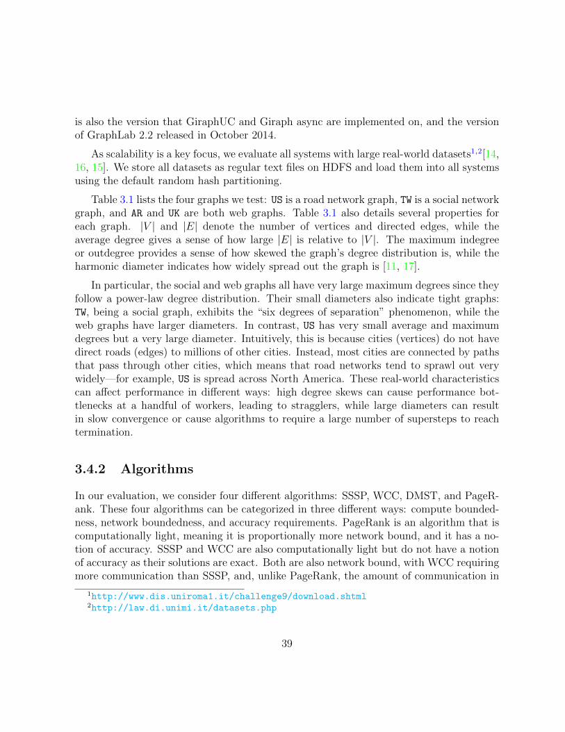
is also the version that GiraphUC and Giraph async are implemented on, and the versionof GraphLab 2.2 released in October 2014.
As scalability is a key focus, we evaluate all systems with large real-world datasets1,2[14,16, 15]. We store all datasets as regular text files on HDFS and load them into all systemsusing the default random hash partitioning.
Table 3.1 lists the four graphs we test: US is a road network graph, TW is a social networkgraph, and AR and UK are both web graphs. Table 3.1 also details several properties foreach graph. |V | and |E| denote the number of vertices and directed edges, while theaverage degree gives a sense of how large |E| is relative to |V |. The maximum indegreeor outdegree provides a sense of how skewed the graph’s degree distribution is, while theharmonic diameter indicates how widely spread out the graph is [11, 17].
In particular, the social and web graphs all have very large maximum degrees since theyfollow a power-law degree distribution. Their small diameters also indicate tight graphs:TW, being a social graph, exhibits the “six degrees of separation” phenomenon, while theweb graphs have larger diameters. In contrast, US has very small average and maximumdegrees but a very large diameter. Intuitively, this is because cities (vertices) do not havedirect roads (edges) to millions of other cities. Instead, most cities are connected by pathsthat pass through other cities, which means that road networks tend to sprawl out verywidely—for example, US is spread across North America. These real-world characteristicscan affect performance in different ways: high degree skews can cause performance bot-tlenecks at a handful of workers, leading to stragglers, while large diameters can resultin slow convergence or cause algorithms to require a large number of supersteps to reachtermination.
3.4.2 Algorithms
In our evaluation, we consider four different algorithms: SSSP, WCC, DMST, and PageR-ank. These four algorithms can be categorized in three different ways: compute bounded-ness, network boundedness, and accuracy requirements. PageRank is an algorithm that iscomputationally light, meaning it is proportionally more network bound, and it has a no-tion of accuracy. SSSP and WCC are also computationally light but do not have a notionof accuracy as their solutions are exact. Both are also network bound, with WCC requiringmore communication than SSSP, and, unlike PageRank, the amount of communication in
1http://www.dis.uniroma1.it/challenge9/download.shtml2http://law.di.unimi.it/datasets.php
39
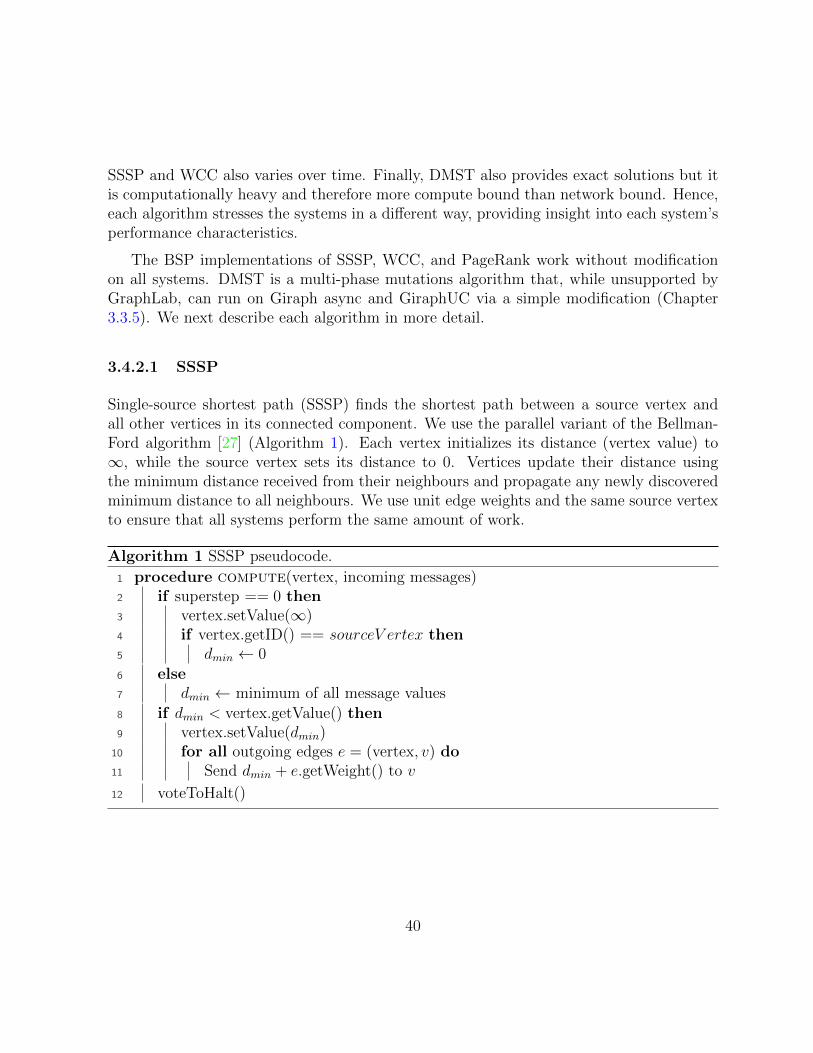
SSSP and WCC also varies over time. Finally, DMST also provides exact solutions but itis computationally heavy and therefore more compute bound than network bound. Hence,each algorithm stresses the systems in a different way, providing insight into each system’sperformance characteristics.
The BSP implementations of SSSP, WCC, and PageRank work without modificationon all systems. DMST is a multi-phase mutations algorithm that, while unsupported byGraphLab, can run on Giraph async and GiraphUC via a simple modification (Chapter3.3.5). We next describe each algorithm in more detail.
3.4.2.1 SSSP
Single-source shortest path (SSSP) finds the shortest path between a source vertex andall other vertices in its connected component. We use the parallel variant of the Bellman-Ford algorithm [27] (Algorithm 1). Each vertex initializes its distance (vertex value) to∞, while the source vertex sets its distance to 0. Vertices update their distance usingthe minimum distance received from their neighbours and propagate any newly discoveredminimum distance to all neighbours. We use unit edge weights and the same source vertexto ensure that all systems perform the same amount of work.
Algorithm 1 SSSP pseudocode.
1 procedure compute(vertex, incoming messages)2 if superstep == 0 then3 vertex.setValue(∞)4 if vertex.getID() == sourceV ertex then5 dmin ← 0
6 else7 dmin ← minimum of all message values
8 if dmin < vertex.getValue() then9 vertex.setValue(dmin)
10 for all outgoing edges e = (vertex, v) do11 Send dmin + e.getWeight() to v
12 voteToHalt()
40
3.4.2.2 WCC
Weakly connected components (WCC) is an algorithm that finds the maximal weaklyconnected components of a graph. A component is weakly connected if all constituentvertices are mutually reachable when ignoring edge directions. We use the HCC algorithm[44], which starts with all vertices initially active (Algorithm 2). Each vertex initializes itscomponent ID (vertex value) to its vertex ID. When a smaller component ID is received,the vertex updates its vertex value to that ID and propagates the ID to its neighbours.We correct GraphLab’s WCC implementation so that it executes correctly in GraphLabasync.
Algorithm 2 WCC pseudocode.
1 procedure compute(vertex, incoming messages)2 if superstep == 0 then3 vertex.setValue(vertex.getID())
4 compIDmin ← minimum of all message values5 if compIDmin < vertex.getValue() then6 vertex.setValue(compIDmin)7 Send compIDmin to vertex’s outgoing neighbours
8 voteToHalt()
3.4.2.3 DMST
Distributed minimum spanning tree (DMST) finds the minimum spanning tree (MST)of an undirected, weighted graph. For unconnected graphs, DMST gives the minimumspanning forest, a union of MSTs. We use the parallel Boruvka algorithm [26, 64] andundirected versions of our datasets weighted with distinct random edge weights. We omitthe pseudocode for DMST due to its complexity.
The algorithm has four different computation phases. In phase one, each vertex selectsa minimum weight out-edge. In phase two, each vertex u uses its selected out-edge and thepointer-jumping algorithm [26] to find its supervertex, a vertex that represents the con-nected component to which u belongs. Phase two requires multiple supersteps to completeand is coordinated using summation aggregators. In phase three, vertices perform edgecleaning by deleting out-edges to neighbours with the same supervertex and modifying theremaining out-edges to point at the supervertex of the edge’s destination vertex. Finally, inphase four, all vertices send their adjacency lists to their supervertex, which merges them
41

according to minimum weight. Vertices designated as supervertices return to phase one asregular vertices, while all other vertices vote to halt. The algorithm terminates when onlyunconnected vertices remain.
The implementation of DMST is over 1300 lines of code and uses custom vertex, edge,and message data types. We add only 4 lines of code to make DMST compatible withGiraphUC and an additional change of 4 more lines of code for Giraph async. As describedin Chapter 3.3.5, these changes are simple and do not affect the algorithm’s logic.
3.4.2.4 PageRank
PageRank is an algorithm that ranks webpages based on the idea that more importantpages receive more links from other pages. Like in [72], we use the accumulative updatePageRank [85] (Algorithm 3). All vertices start with a value of 0.0. At each superstep,a vertex u sets delta to be the sum of all values received from its in-edges (or 0.15 inthe first superstep), and its PageRank value pr(u) to be pr(u) + delta. It then sends0.85 · delta/ deg+(u) along its out-edges, where deg+(u) is u’s outdegree. The algorithmterminates after a user-specified K supersteps, and each output pr(u) gives the expectationvalue for a vertex u. The probability value can be obtained by dividing the expectationvalue by the number of vertices.
Algorithm 3 PageRank pseudocode.
1 procedure compute(vertex, incoming messages)2 if superstep == 0 then3 vertex.setValue(0)4 delta← 0.155 else6 delta← sum of all message values
7 vertex.setValue(vertex.currValue() + delta)8 if superstep ≤ K then9 m← number of outgoing edges of vertex
10 Send 0.85 · delta/m to all outgoing neighbours11 else12 voteToHalt()
All systems except GraphLab async terminate after a fixed number of (logical) super-steps, as this provides the best accuracy and performance. GraphLab async, which has no
42
notion of supersteps, terminates after the PageRank value of every vertex u changes byless than a user-specified threshold ε between two consecutive executions of u.
3.4.3 Results
For our results, we focus on computation time, which is the total time of running an algo-rithm minus the input loading and output writing times. Computation time hence includestime spent on vertex computation, barrier synchronization, and network communication.This means, for example, it captures network performance: poor utilization of networkresources translates to poor (longer) computation time. Since computation time captureseverything that is affected by using different computation models, it accurately reflects theperformance differences between each system.
For SSSP, WCC, and DMST (Figure 3.6), we report the mean and 95% confidenceintervals of five runs. For PageRank (Figure 3.7), each data point is the mean of five runs,with 95% confidence intervals shown as vertical and horizontal error bars for both accuracyand time. Additionally, we ensure correctness by comparing the outputs of GiraphUC andGiraph async to that of Giraph sync. In total, we perform over 700 experimental runs.
3.4.3.1 SSSP
GiraphUC outperforms all of the other systems for SSSP on all datasets (Figure 3.6a).This performance gap is particularly large on US, which requires thousands of superstepsto complete due to the graph’s large diameter (Table 3.1). By reducing per-superstepoverheads, GiraphUC is up to 4.5× faster than Giraph sync, Giraph async, and GraphLabsync. Giraph async performs poorly due to the high per-superstep overheads of usingglobal barriers. GraphLab async fails on US after 2 hours (7200s), indicated by an ‘F’in Figure 3.6a, due to machines running out of memory during its distributed consensustermination. This demonstrates that GiraphUC’s two step termination check has superiorscalability.
On AR, TW, and UK, GiraphUC continues to provide gains. For example, it is up to3.5× faster than Giraph sync, Giraph async, and GraphLab sync on AR. GraphLab asyncsuccessfully runs on these graphs but its computation times are highly variable (Figure 3.6a)due to highly variable network overheads. These overheads are due to GraphLab async’slack of message batching and its pairing of fibers to individual vertices (Chapter 2.1.3),which results in highly non-deterministic execution compared to GiraphUC’s approach ofpairing compute threads with partitions (Chapter 3.3.1). GraphLab async’s poor scalability
43
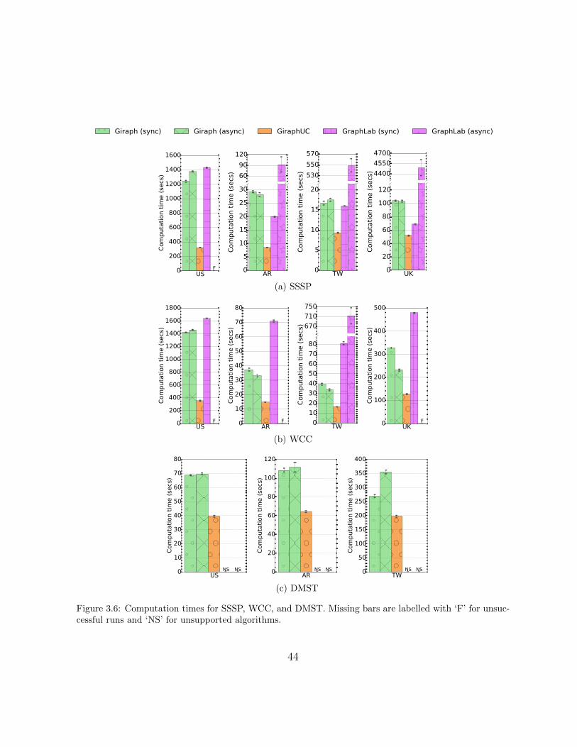
Giraph (sync) Giraph (async) GiraphUC GraphLab (sync) GraphLab (async)
US0
200
400
600
800
1000
1200
1400
1600Computation tim
e (secs)
F 0
100
Computation tim
e (secs) 60
90
120
AR0
5
10
15
20
25
30
0.0
10.1
Computation tim
e (secs) 530
550
570
TW0
5
10
15
20
0
1000
Computation tim
e (secs) 4400
4550
4700
UK0
20
40
60
80
100
120
(a) SSSP
US0
200
400
600
800
1000
1200
1400
1600
1800
Computation tim
e (secs)
FAR0
10
20
30
40
50
60
70
80
Computation tim
e (secs)
F 0
100Computation tim
e (secs) 670
710
750
TW0
10
20
30
40
50
60
70
80
UK0
100
200
300
400
500
Computation tim
e (secs)
F
(b) WCC
US0
10
20
30
40
50
60
70
80
Computation tim
e (secs)
NS NSAR
0
20
40
60
80
100
120
Computation tim
e (secs)
NS NSTW
0
50
100
150
200
250
300
350
400
Computation tim
e (secs)
NS NS
(c) DMST
Figure 3.6: Computation times for SSSP, WCC, and DMST. Missing bars are labelled with ‘F’ for unsuc-cessful runs and ‘NS’ for unsupported algorithms.
44
is especially evident on TW and UK, where GiraphUC outperforms it by 59× and 86×respectively. Hence, GiraphUC is more scalable and does not suffer the communicationoverheads caused by GraphLab async’s lack of message batching and its use of distributedlocking and distributed consensus termination.
3.4.3.2 WCC
For WCC, GiraphUC consistently outperforms all of the other systems on all graphs: up to4× versus Giraph sync and async on US, and nearly 5× versus GraphLab sync on TW (Figure3.6b). In particular, whenever Giraph async has gains over Giraph sync, such as on UK,GiraphUC further improves on Giraph async’s performance. In cases where Giraph asyncperforms poorly, such as on US, GiraphUC still performs better than Giraph sync. Thisshows that the BAP model implemented by GiraphUC provides substantial improvementsover the eAP model used by Giraph async.
Finally, like in SSSP, GraphLab async again performs poorly at scale: it fails on US
after 5 hours (18,000s), AR after 20 minutes (1200s), and UK after 40 minutes (2400s) due toexhausting the available memory at several worker machines. For TW, on which GraphLabasync successfully runs, GiraphUC is still 43× faster (Figure 3.6b).
3.4.3.3 DMST
For DMST, GiraphUC is 1.7× faster than both Giraph sync and async on US and AR, and1.4× and 1.8× faster than Giraph sync and async respectively on TW (Figure 3.6c). Theseperformance gains are primarily achieved in the second computation phase of DMST, whichtypically requires many supersteps to complete (Chapter 3.4.2.3). GiraphUC’s gains areslightly lower than in SSSP and WCC because DMST is more compute bound, which meansproportionally less time spent on communication and barriers. This is particularly true forTW, whose extreme degree skew leads to more computation time spent performing graphmutations. Nevertheless, GiraphUC’s good performance establishes its effectiveness alsofor compute bound algorithms and algorithms that require multiple computation phases.
Giraph sync, Giraph async, and GiraphUC, when running DMST on UK, all exhaust thememory of several worker machines due to the size of the undirected weighted version ofthe graph. However, we expect trends to be similar since UK has a less extreme degree skewthan TW (Table 3.1), meaning DMST will be less compute bound and can hence benefitmore under GiraphUC.
45
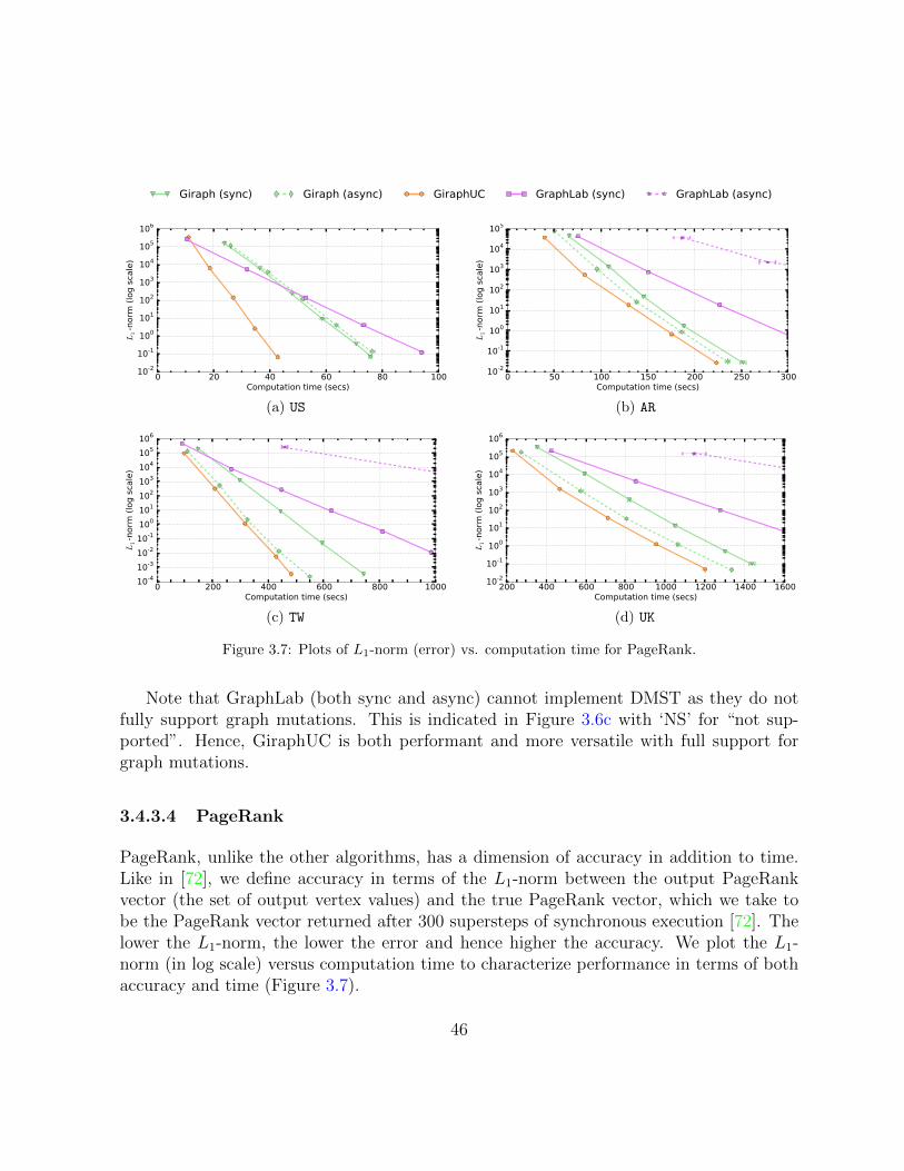
Giraph (sync) Giraph (async) GiraphUC GraphLab (sync) GraphLab (async)
0 20 40 60 80 100Computation time (secs)
10-2
10-1
100
101
102
103
104
105
106
L1-norm
(log sca
le)
(a) US
0 50 100 150 200 250 300Computation time (secs)
10-2
10-1
100
101
102
103
104
105
L1-norm
(log sca
le)
(b) AR
0 200 400 600 800 1000Computation time (secs)
10-4
10-3
10-2
10-1
100
101
102
103
104
105
106
L1-norm
(log sca
le)
(c) TW
200 400 600 800 1000 1200 1400 1600Computation time (secs)
10-2
10-1
100
101
102
103
104
105
106
L1-norm
(log sca
le)
(d) UK
Figure 3.7: Plots of L1-norm (error) vs. computation time for PageRank.
Note that GraphLab (both sync and async) cannot implement DMST as they do notfully support graph mutations. This is indicated in Figure 3.6c with ‘NS’ for “not sup-ported”. Hence, GiraphUC is both performant and more versatile with full support forgraph mutations.
3.4.3.4 PageRank
PageRank, unlike the other algorithms, has a dimension of accuracy in addition to time.Like in [72], we define accuracy in terms of the L1-norm between the output PageRankvector (the set of output vertex values) and the true PageRank vector, which we take tobe the PageRank vector returned after 300 supersteps of synchronous execution [72]. Thelower the L1-norm, the lower the error and hence higher the accuracy. We plot the L1-norm (in log scale) versus computation time to characterize performance in terms of bothaccuracy and time (Figure 3.7).
46
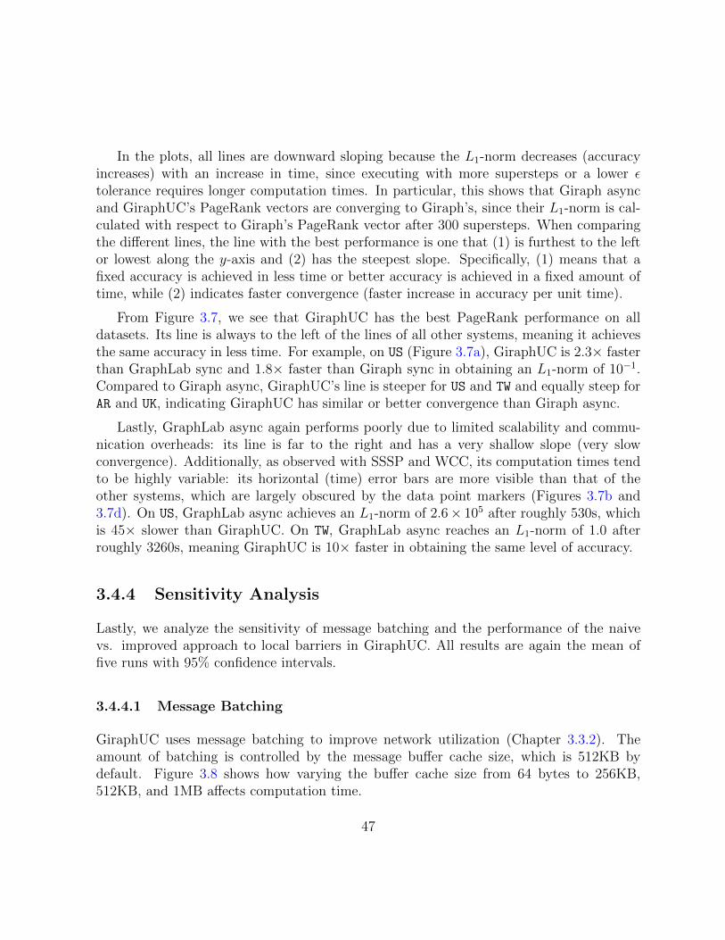
In the plots, all lines are downward sloping because the L1-norm decreases (accuracyincreases) with an increase in time, since executing with more supersteps or a lower εtolerance requires longer computation times. In particular, this shows that Giraph asyncand GiraphUC’s PageRank vectors are converging to Giraph’s, since their L1-norm is cal-culated with respect to Giraph’s PageRank vector after 300 supersteps. When comparingthe different lines, the line with the best performance is one that (1) is furthest to the leftor lowest along the y-axis and (2) has the steepest slope. Specifically, (1) means that afixed accuracy is achieved in less time or better accuracy is achieved in a fixed amount oftime, while (2) indicates faster convergence (faster increase in accuracy per unit time).
From Figure 3.7, we see that GiraphUC has the best PageRank performance on alldatasets. Its line is always to the left of the lines of all other systems, meaning it achievesthe same accuracy in less time. For example, on US (Figure 3.7a), GiraphUC is 2.3× fasterthan GraphLab sync and 1.8× faster than Giraph sync in obtaining an L1-norm of 10−1.Compared to Giraph async, GiraphUC’s line is steeper for US and TW and equally steep forAR and UK, indicating GiraphUC has similar or better convergence than Giraph async.
Lastly, GraphLab async again performs poorly due to limited scalability and commu-nication overheads: its line is far to the right and has a very shallow slope (very slowconvergence). Additionally, as observed with SSSP and WCC, its computation times tendto be highly variable: its horizontal (time) error bars are more visible than that of theother systems, which are largely obscured by the data point markers (Figures 3.7b and3.7d). On US, GraphLab async achieves an L1-norm of 2.6× 10⁵ after roughly 530s, whichis 45× slower than GiraphUC. On TW, GraphLab async reaches an L1-norm of 1.0 afterroughly 3260s, meaning GiraphUC is 10× faster in obtaining the same level of accuracy.
3.4.4 Sensitivity Analysis
Lastly, we analyze the sensitivity of message batching and the performance of the naivevs. improved approach to local barriers in GiraphUC. All results are again the mean offive runs with 95% confidence intervals.
3.4.4.1 Message Batching
GiraphUC uses message batching to improve network utilization (Chapter 3.3.2). Theamount of batching is controlled by the message buffer cache size, which is 512KB bydefault. Figure 3.8 shows how varying the buffer cache size from 64 bytes to 256KB,512KB, and 1MB affects computation time.
47
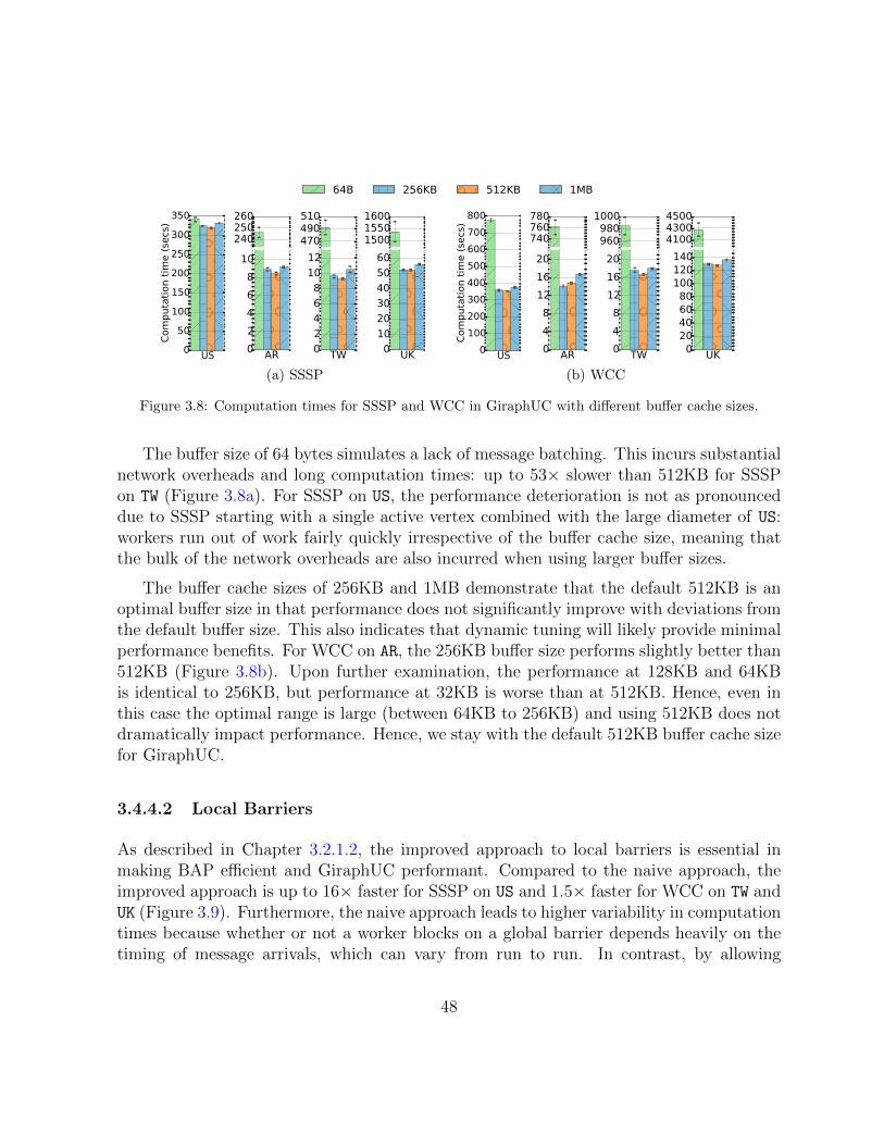
64B 256KB 512KB 1MB
US0
50
100
150
200
250
300
350
Computation tim
e (secs)
0.0
10.1
240250260
AR0
2
4
6
8
10
0.0
10.1
470490510
TW0
2
4
6
8
10
12
0
1000
150015501600
UK0
10
20
30
40
50
60
(a) SSSP
US0
100
200
300
400
500
600
700
800
Computation tim
e (secs)
0.0
10.1
740760780
AR0
4
8
12
16
20
0.0
10.1
9609801000
TW0
4
8
12
16
20
0
1000
410043004500
UK020406080100120140
(b) WCC
Figure 3.8: Computation times for SSSP and WCC in GiraphUC with different buffer cache sizes.
The buffer size of 64 bytes simulates a lack of message batching. This incurs substantialnetwork overheads and long computation times: up to 53× slower than 512KB for SSSPon TW (Figure 3.8a). For SSSP on US, the performance deterioration is not as pronounceddue to SSSP starting with a single active vertex combined with the large diameter of US:workers run out of work fairly quickly irrespective of the buffer cache size, meaning thatthe bulk of the network overheads are also incurred when using larger buffer sizes.
The buffer cache sizes of 256KB and 1MB demonstrate that the default 512KB is anoptimal buffer size in that performance does not significantly improve with deviations fromthe default buffer size. This also indicates that dynamic tuning will likely provide minimalperformance benefits. For WCC on AR, the 256KB buffer size performs slightly better than512KB (Figure 3.8b). Upon further examination, the performance at 128KB and 64KBis identical to 256KB, but performance at 32KB is worse than at 512KB. Hence, even inthis case the optimal range is large (between 64KB to 256KB) and using 512KB does notdramatically impact performance. Hence, we stay with the default 512KB buffer cache sizefor GiraphUC.
3.4.4.2 Local Barriers
As described in Chapter 3.2.1.2, the improved approach to local barriers is essential inmaking BAP efficient and GiraphUC performant. Compared to the naive approach, theimproved approach is up to 16× faster for SSSP on US and 1.5× faster for WCC on TW andUK (Figure 3.9). Furthermore, the naive approach leads to higher variability in computationtimes because whether or not a worker blocks on a global barrier depends heavily on thetiming of message arrivals, which can vary from run to run. In contrast, by allowing
48
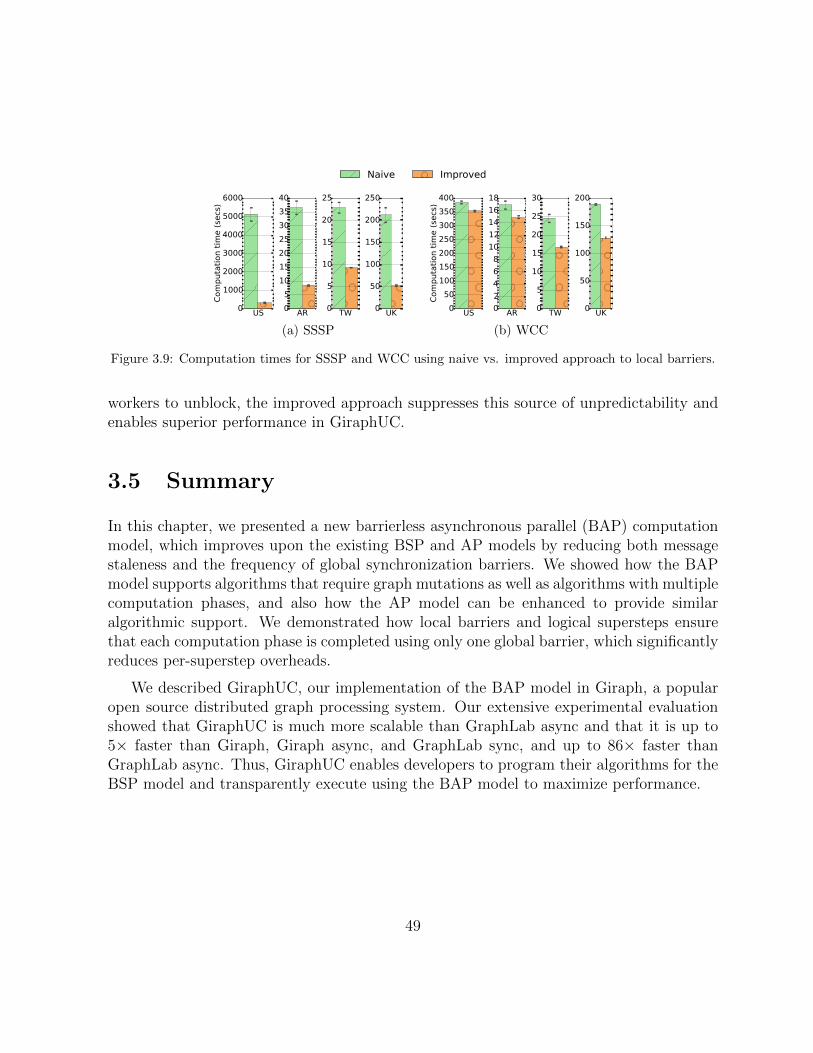
Naive Improved
US0
1000
2000
3000
4000
5000
6000
Computation tim
e (secs)
AR0
5
10
15
20
25
30
35
40
TW0
5
10
15
20
25
UK0
50
100
150
200
250
(a) SSSP
US0
50
100
150
200
250
300
350
400
Computation tim
e (secs)
AR0
2
4
6
8
10
12
14
16
18
TW0
5
10
15
20
25
30
UK0
50
100
150
200
(b) WCC
Figure 3.9: Computation times for SSSP and WCC using naive vs. improved approach to local barriers.
workers to unblock, the improved approach suppresses this source of unpredictability andenables superior performance in GiraphUC.
3.5 Summary
In this chapter, we presented a new barrierless asynchronous parallel (BAP) computationmodel, which improves upon the existing BSP and AP models by reducing both messagestaleness and the frequency of global synchronization barriers. We showed how the BAPmodel supports algorithms that require graph mutations as well as algorithms with multiplecomputation phases, and also how the AP model can be enhanced to provide similaralgorithmic support. We demonstrated how local barriers and logical supersteps ensurethat each computation phase is completed using only one global barrier, which significantlyreduces per-superstep overheads.
We described GiraphUC, our implementation of the BAP model in Giraph, a popularopen source distributed graph processing system. Our extensive experimental evaluationshowed that GiraphUC is much more scalable than GraphLab async and that it is up to5× faster than Giraph, Giraph async, and GraphLab sync, and up to 86× faster thanGraphLab async. Thus, GiraphUC enables developers to program their algorithms for theBSP model and transparently execute using the BAP model to maximize performance.
49
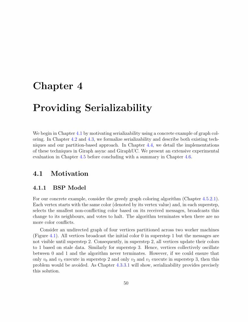
Chapter 4
Providing Serializability
We begin in Chapter 4.1 by motivating serializability using a concrete example of graph col-oring. In Chapter 4.2 and 4.3, we formalize serializability and describe both existing tech-niques and our partition-based approach. In Chapter 4.4, we detail the implementationsof these techniques in Giraph async and GiraphUC. We present an extensive experimentalevaluation in Chapter 4.5 before concluding with a summary in Chapter 4.6.
4.1 Motivation
4.1.1 BSP Model
For our concrete example, consider the greedy graph coloring algorithm (Chapter 4.5.2.1).Each vertex starts with the same color (denoted by its vertex value) and, in each superstep,selects the smallest non-conflicting color based on its received messages, broadcasts thischange to its neighbours, and votes to halt. The algorithm terminates when there are nomore color conflicts.
Consider an undirected graph of four vertices partitioned across two worker machines(Figure 4.1). All vertices broadcast the initial color 0 in superstep 1 but the messages arenot visible until superstep 2. Consequently, in superstep 2, all vertices update their colorsto 1 based on stale data. Similarly for superstep 3. Hence, vertices collectively oscillatebetween 0 and 1 and the algorithm never terminates. However, if we could ensure thatonly v0 and v3 execute in superstep 2 and only v2 and v1 execute in superstep 3, then thisproblem would be avoided. As Chapter 4.3.3.1 will show, serializability provides preciselythis solution.
50
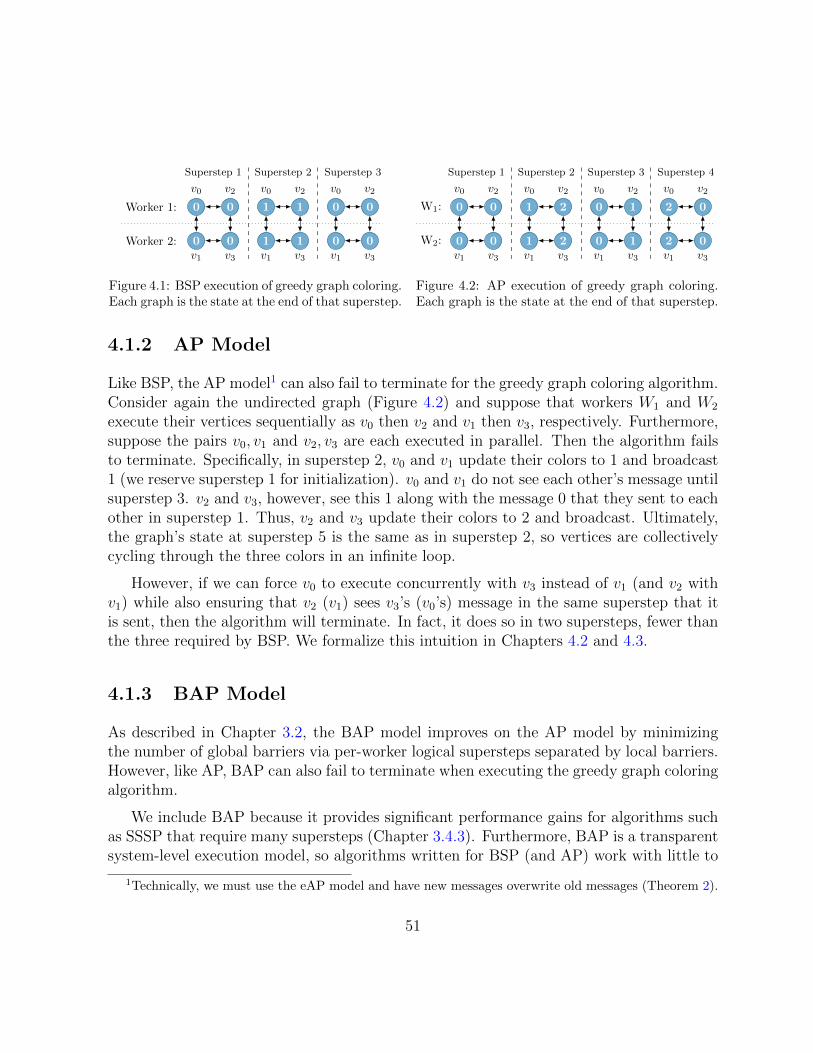
Worker 1:
Worker 2:
0
0
0
0
v0 v2
v1 v3
Superstep 1
1
1
1
1
v0 v2
v1 v3
Superstep 2
0
0
0
0
v0 v2
v1 v3
Superstep 3
Figure 4.1: BSP execution of greedy graph coloring.Each graph is the state at the end of that superstep.
W1:
W2:
0
0
0
0
v0 v2
v1 v3
Superstep 1
1
1
2
2
v0 v2
v1 v3
Superstep 2
0
0
1
1
v0 v2
v1 v3
Superstep 3
2
2
0
0
v0 v2
v1 v3
Superstep 4
Figure 4.2: AP execution of greedy graph coloring.Each graph is the state at the end of that superstep.
4.1.2 AP Model
Like BSP, the AP model1 can also fail to terminate for the greedy graph coloring algorithm.Consider again the undirected graph (Figure 4.2) and suppose that workers W1 and W2
execute their vertices sequentially as v0 then v2 and v1 then v3, respectively. Furthermore,suppose the pairs v0, v1 and v2, v3 are each executed in parallel. Then the algorithm failsto terminate. Specifically, in superstep 2, v0 and v1 update their colors to 1 and broadcast1 (we reserve superstep 1 for initialization). v0 and v1 do not see each other’s message untilsuperstep 3. v2 and v3, however, see this 1 along with the message 0 that they sent to eachother in superstep 1. Thus, v2 and v3 update their colors to 2 and broadcast. Ultimately,the graph’s state at superstep 5 is the same as in superstep 2, so vertices are collectivelycycling through the three colors in an infinite loop.
However, if we can force v0 to execute concurrently with v3 instead of v1 (and v2 withv1) while also ensuring that v2 (v1) sees v3’s (v0’s) message in the same superstep that itis sent, then the algorithm will terminate. In fact, it does so in two supersteps, fewer thanthe three required by BSP. We formalize this intuition in Chapters 4.2 and 4.3.
4.1.3 BAP Model
As described in Chapter 3.2, the BAP model improves on the AP model by minimizingthe number of global barriers via per-worker logical supersteps separated by local barriers.However, like AP, BAP can also fail to terminate when executing the greedy graph coloringalgorithm.
We include BAP because it provides significant performance gains for algorithms suchas SSSP that require many supersteps (Chapter 3.4.3). Furthermore, BAP is a transparentsystem-level execution model, so algorithms written for BSP (and AP) work with little to
1Technically, we must use the eAP model and have new messages overwrite old messages (Theorem 2).
51
no modifications (Chapter 3.2). In fact, the techniques for providing serializability areidentical for both the AP and BAP models (Chapter 4.3).
4.1.4 GAS Model
As described in Chapter 2.1.3, sync GAS is similar to BSP and so fails to terminate in thesame way (Figure 4.1), while async GAS can fail to terminate in the case of dense graphs[34]. For example, for the graph coloring example in Figure 4.2, suppose both W1 andW2 each have two threads for their two vertices and all threads run in parallel. Then theinterleaving of the GAS phases will cause vertices to see stale colors and so the executionis not guaranteed to terminate: it can become stuck in an infinite loop. In contrast, byadding the vertex-based distributed locking technique (Chapter 2.1.3), async GAS withserializability will always terminate successfully.
4.2 Serializability
In this section, we formally define serializability and prove several key properties.
4.2.1 Preliminaries
Existing work [34, 71] considers serializability for algorithms where vertices communicateonly with their direct neighbours, which is the behaviour of the majority of algorithms thatrequire serializability. For example, the GAS model supports only algorithms where verticescommunicate with their direct neighbours [50, 34]. For these algorithms, serializability canbe provided transparently by the graph processing system, independent of the algorithmbeing executed. Thus, our focus is on these types of algorithms.
Since popular graph processing systems use a vertex-centric programming model, wheredevelopers specify the actions of a single vertex, we focus on vertex-centric systems. Theformalisms that we will establish apply to all vertex-centric systems, irrespective of thecomputation models they use.
In vertex-centric graph processing systems, there are two levels of parallelism: (1)between multiple threads within a single worker machine and (2) between the multipleworker machines. Due to the distributed nature of computation, the input graph must bepartitioned across the workers and so data replication will occur. To better understandthis, let neighbours refer to both in-edge and out-edge neighbours.
52
Definition 1. A vertex u is a machine boundary vertex, or m-boundary for short, if atleast one of its neighbours v belongs to a different worker machine from u. Otherwise, uis a machine internal, or m-internal, vertex.
Definition 2. A replica is local if it belongs to the same worker machine as its primarycopy and remote otherwise.
Systems keep a read-only replica of each vertex on its owner’s machine and of eachm-boundary vertex u on each of u’s out-edge neighbour’s worker machines. This is astandard design used, for example, in Pregel, Giraph, and GraphLab. Remote replicas(of m-boundary vertices) exist due to graph partitioning: for vertex-cut partitioning, u’svertex value is explicitly replicated on every out-edge neighbour v’s worker machine; foredge-cut, u is implicitly replicated because the message it sends to v, which is a function ofu’s vertex value, is buffered in the message store of v’s machine. This distinction is unim-portant for our formalism as we care only about whether replication occurs. Local replicasoccur in push-based systems because message stores also buffer messages sent between ver-tices belonging to the same worker. In pull-based systems, local replicas are required forimplementing synchronous computation models like sync GAS. For asynchronous models,pull-based systems may not always have local replicas (such as in GraphLab async) butwe will consider the more general case in which they do (if they do not, then reads of suchvertices will always trivially see up-to-date data).
Definition 3. A read of a replica is fresh if the replica is up-to-date with its primary copyand stale otherwise.
Informally, an execution is serializable if it produces the same result as a serial executionin which all reads are fresh. More formally, we require one-copy serializability (1SR) [13].
Definition 4. A system provides serializability, or serializable executions, if and only ifall executions produce histories that are one-copy serializable (1SR).
In the subsequent sections, we prove that 1SR can be provided by enforcing two condi-tions: (1) all vertices read up-to-date replicas of its in-edge neighbours prior to executionand (2) no vertex has executions that are concurrent with any of its in-edge neighbours.In terms of traditional transaction terminology, we define a site as a worker machine, anitem as a vertex, and a transaction as the execution of a single vertex. We detail suchtransactions next.
53
4.2.2 Transactions
We define a transaction to be the single execution of an arbitrary vertex u, consisting ofa read on u and the replicas of u’s in-edge neighbours followed by a write to u. The readacts only on u and its in-edge neighbours because u receives messages (or pulls data) fromonly its in-edge neighbours—it has no dependency on its out-edge neighbours. Denotingthe read set as Nu = {u, u’s in-edge neighbours}, any execution of u is the transactionTi = ri[Nu]wi[u], or simply Ti(Nu) as all transactions are of the same form.
Any v ∈ Nu with v 6= u is also annotated to distinguish it from the other read-onlyreplicas of v. For example, if u belongs to worker A, we annotate the read-only replica asvA ∈ Nu. However, the next section will show how we can drop these annotations.
Our definition relies only on the fact that the system is vertex-centric and not on thenuances of specific computation models. For example, although BSP and AP have a notionof supersteps, the i for a transaction Ti(Nu) has no relation to the superstep count. Theexecution of u in two different supersteps is represented by two different transactions Ti(Nu)and Tj(Nu). Our definitions also work when there is no notion of supersteps, such as inthe async GAS model, or when there are only per-worker logical supersteps, such as in theBAP model.
We can now restate our two conditions more formally as:
Condition C1. Before any transaction Ti(Nu) executes, all replicas v ∈ Nu on u’smachine are up-to-date.
Condition C2. No transaction Ti(Nu) overlaps with any transaction Tj(Nv) for allcopies of v ∈ Nu, v 6= u.
4.2.3 Replicated Data
We first show how to enforce condition C1 and then prove, in Lemma 1, that enforcingcondition C1 simplifies the problem to standard serializability on a single logical copy ofeach vertex (i.e., without data replication).
We enforce condition C1 by combining a write-all approach [13] with a synchronizationtechnique that ensures neighbouring vertices do not execute concurrently. Denote u’s in-edge and out-edge neighbours as Mu. Then a synchronization technique prevents stalereads by ensuring no transactions Tj(Nv) with any copy of v ∈ Mu occur while updates
54
are being propagated to u’s replicas. In theory, the write-all approach must update replicaseagerly: Ti(Nu) commits only after all replicas of u are synchronously updated. In practice,vertices coordinated by a synchronization technique can update their replicas lazily, becauseany such vertex v must first acquire a shared resource (e.g., a token or a fork) from itsneighbour u before it can execute. Thus, updates to u’s replicas can be delayed and insteadsent before handing over the resource required by v. The effect is the same as an eagerwrite-all approach: v always reads an up-to-date replica of u. Chapter 4.3.1.1 describesthis approach in greater detail.
The write-all approach works for graph processing systems because we replicate fordistributed computation, not for availability. That is, when a worker machine fails, welose a portion of our input graph and so we cannot proceed with the computation. Indeed,failure recovery requires all machines to rollback to a previous checkpoint [1, 50, 54],meaning pending writes to failed machines do not occur.
Lemma 1. If condition C1 is true, then it suffices to use standard serializability theorywhere operations are performed on a single logical copy of each vertex.
Proof. Condition C1 ensures that before every transaction Ti(Nu) executes, the replicasv ∈ Nu are all up-to-date. Then all reads ri[Nu] see up-to-date replicas and are thus thesame as reading from the primary copy of each v ∈ Nu. Hence, there is effectively only asingle logical copy of each vertex, so we can apply standard serializability theory.
4.2.4 Correctness
We use the standard notion of conflicts and histories [13]. Two transactions conflict if theyhave conflicting operations. We assume, per Lemma 1, that reads and writes are performedon a single logical copy of each vertex.
A serial single-copy history produced by the serial execution of an algorithm is a se-quence of transactions where operations act on a single logical copy and do not interleave.For example, one possible serial single-copy history for two vertices u and v would be
r1[Nu]w1[u]c1r2[Nv]w2[v]c2r3[Nu]w3[u]c3r4[Nv]w4[v]c4,
where ci denotes the commit of each transaction. Irrespective of the computation model,the history indicates that u and v are each executed twice before the algorithm terminates.If the computation model has a notion of supersteps, and we assume that u and v areexecuted exactly once in each superstep, then T1 and T2 would belong to the first superstepwhile T3 and T4 would belong to the second.
55
As per Definition 4, we require 1SR. We first prove a useful relationship between inputand serializability graphs (Lemma 2) before formally defining the relationship betweenserializability and conditions C1 and C2 (Theorem 4).
Lemma 2. Suppose condition C1 is true. Then a directed cycle of ≥ 2 vertices exists inthe input graph if and only if there exists an execution that produces a serialization graphcontaining a directed cycle.
Proof. Since condition C1 holds, by Lemma 1 we can apply standard serializability theory.
(Only if) Suppose the input graph contains a directed cycle of n ≥ 2 vertices and, with-out loss of generality, assume that the cycle is formed by the edges (un, u1) and (ui, ui+1)for i ∈ [1, n). Consider executions in which all read operations occur before any writeoperation. That is, consider histories of the form r1[Nu1 ] · · · rn[Nun ]w1[u1]c1 · · ·wn[un]cnwhere operations can be arbitrarily permuted so long as all reads precede all writes. Thisdoes not violate condition C1 because all reads are fresh.
Recall that the serialization graph of a history consists of a node for each transactionand an edge from Ti to Tj if one of Ti’s operations precedes and conflicts with one of Tj’soperations [13]. Since all reads occur before writes, every transaction Ti’s read operationri[Nui
] will precede and conflict with transaction Ti−1’s write operation wi−1[ui−1] for i ∈(1, n] because ui−1 ∈ Nui
. That is, there exists a directed path from Tn to T1 in theserialization graph. Additionally, because of the directed cycle in the input graph, we alsohave a conflict due to un ∈ Nu1 . This adds an edge from T1 to Tn which, together with thedirected path from Tn to T1, creates a directed cycle in the serialization graph. Hence, allhistories of this form produce serialization graphs with a directed cycle.2
(If) For the converse, suppose there exists a cycle in the serialization graph. Thenthere exist two transactions Ti(Nu) and Tj(Nv), for arbitrary i, j and vertices u, v, thatmust be ordered as Tj(Nv) < Ti(Nu) and Ti(Nu) < · · · < Tj(Nv).
The former ordering can only be due to rj[Nv] < wi[u], since every transaction has itsread precede its write, which implies that u ∈ Nv and so there exists an edge (u, v) in theinput graph. Similarly, the latter ordering implies that there is a directed path from v tou. For example, suppose the ordering is Ti(Nu) < Tk(Nw) < Tj(Nv). Then this must arise
2Another proof can also be achieved using induction. For example, histories of the form
rn[Nun]rn−1[Nun−1
] · · · r1[Nu1]w1[u1]c1 · · ·wn[un]cn
will always require Tn < Tn−1 < · · · < T1, because ui ∈ Nui+1for i ∈ [1, n), and T1 < Tn since un ∈ Nu1
.The two orderings then create a cycle in the serialization graph.
56
due to ri[Nu] < wk[w] and rk[Nw] < wj[v], meaning w ∈ Nu and v ∈ Nw. Equivalently,there exist edges (w, u) and (v, w) in the input graph and thus a directed path from v tou. In general, the more transactions there are between Ti(Nu) and Tj(Nv), the longer thispath.
Since there is both a directed path from v to u and an edge (u, v), the input graph hasa directed cycle.
Theorem 4. All executions are serializable for all input graphs if and only if conditionsC1 and C2 are both true.
Proof. (If) Since condition C1 is true, by Lemma 1 we can apply standard serializabilitytheory. By the serializability theorem [13], it suffices to show if condition C2 is true thenall possible histories have an acyclic serialization graph.
Consider two arbitrary concurrent transactions Ti(Nu) and Tj(Nv). For vertex-centricsystems, each vertex is always executed by exactly one thread of execution because thecompute function is written for serial execution. That is, we must have u 6= v for Ti andTj. Since condition C2 is true, the write operations of Ti and Tj are always on u /∈ Nv
and v /∈ Nu, respectively, meaning the transactions do not conflict. That is, condition C2eliminates all conflicting transactions from all possible histories, so the serialization graphmust be acyclic. Since we make no assumptions about the input graph, this holds for allinput graphs.
(Only if) Next, we prove the inverse: if either condition C1 or C2 is false, then thereexists a non-serializable execution for some input graph. Consider an input graph withvertices u and v connected by an undirected edge and executed by the transactions T1(Nu)and T2(Nv), respectively.
Suppose C1 is true but C2 is not. Then T1(Nu) and T2(Nv) can execute in paralleland so a possible history is r1[Nu]r2[Nv]w1[u]c1w2[v]c2. This history does not violate C1because both reads see up-to-date state. However, the two transactions conflict: v ∈ Nu
implies T1 < T2 while u ∈ Nv implies T2 < T1, so this execution is not serializable. Moregenerally, per Lemma 2, this occurs for any graph with a directed cycle of ≥ 2 vertices.
Suppose C2 is true but C1 is not. Then standard serializability no longer applies asthere are now replicas. For our input graph, let u be at worker A and v be at workerB. Then Nu = {u, vA} and Nv = {v, uB}, where vA and uB are replicas of v and urespectively. Consider a serial history r1[{u, vA}]w1[u]c1r2[{v, uB}]w2[v]c2 where initiallyvA = v and uB = u, but uB 6= u after T1. This history is possible under condition C2 (itis serial) but it is not 1SR: vA = v implies T1 < T2 while uB 6= u implies T2 < T1, so there
57
are no conflict equivalent serial single-copy histories. Another way to see this is that theabove history is effectively a concurrent execution of T1 and T2 on a single copy of u andv—i.e., where condition C1 is true but C2 is not.
Lastly, we note a theoretically interesting corollary.
Corollary 1. Suppose condition C1 is true. Then all executions are serializable if andonly if the input graph has no directed cycles of ≥ 2 vertices.
Proof. This is just the contrapositive of Lemma 2: there are no directed cycles of ≥ 2vertices in the input graph iff there are no executions that produce a serialization graphcontaining a cycle. Applying the serializability theorem, we have: all executions are seri-alizable iff the input graph has no directed cycles of ≥ 2 vertices.3
However, in practice, Corollary 1 is insufficient for providing serializability becausenearly all real world graphs have at least one undirected edge. Moreover, the synchroniza-tion technique used to enforce condition C1 will also enforce condition C2 (Chapters 4.2.3and 4.2.5).
4.2.5 Enforcing Serializability
Graph processing systems that implement any of the computation models from Chapter2.1 do not enforce conditions C1 and C2 as none of the models utilize any synchronizationtechniques. Hence, by Theorem 4, they do not provide serializability. Moreover, thesesystems do not guarantee fresh reads even under serial executions (on a single machineor under the sequential execution of multiple machines). For example, BSP effectivelyupdates replicas lazily4 because messages sent in one superstep, even if received, cannotbe read by the recipient in the same superstep. Thus, both m-boundary and m-internalvertices (Definition 1) suffer stale reads under a serial execution. While AP weakens thisisolation and can update local replicas eagerly, it propagates messages to remote replicaslazily without the guarantees of condition C1 and so stale reads can again occur under aserial execution of multiple machines.
3Self-cycles in the input graph are permitted because a single vertex is executed by one thread ofexecution at any time (see the proof of Theorem 4).
4The “synchronous” in BSP refers to the global communication barriers, not the method of replicasynchronization.
58
To provide serializability, we enforce conditions C1 and C2 by adding a synchronizationtechnique (Chapter 4.3) to the systems that implement the above computation models. Forexample, GraphLab async provides serializability by adding a distributed locking synchro-nization technique on top of the async GAS model. These synchronization techniques alsoimplement a write-all approach for updating replicas, which is required for condition C1.
The synchronization techniques ensure that a vertex u does not execute concurrentlywith any of its in-edge and out-edge neighbours. At first glance, this appears to be strongerthan what condition C2 requires. However, suppose v is an out-edge neighbour of u andv is currently executing. Then if u does not synchronize with its out-edge neighbours, itwill erroneously execute concurrently with v, violating condition C2 for v. Alternatively,if v is an out-edge neighbour of u then u is an in-edge neighbour of v, so they must notexecute concurrently.
4.3 Synchronization Techniques
In this section, we describe synchronization techniques to enforce conditions C1 and C2 aswell as their performance with respect to parallelism and communication overheads.
4.3.1 Preliminaries
4.3.1.1 Replica Updates
How a synchronization technique implements the write-all approach (Chapter 4.2.3) de-pends on whether the computation model is synchronous or asynchronous.
For asynchronous computation models (AP, BAP, async GAS), replicas immediatelyapply received updates. Thus, local replicas can be updated eagerly, since there are nocommunication costs (Chapter 4.4). Remote replicas, however, are updated lazily in ajust-in-time fashion to provide communication batching: if an m-boundary vertex u has areplica on its neighbour v’s worker then, when v wants to execute, u’s worker will flush allpending remote replica updates before handing over the shared resource that allows v toproceed.
In contrast, synchronous computation models (BSP, sync GAS) hide updates fromreplicas until the next superstep. That is, replicas can only be updated after a globalbarrier. This means systems with synchronous models are limited to specialized synchro-nization techniques that keep replicas up-to-date by dividing each superstep into multiple
59
sub-supersteps (Proposition 2). This is significantly less performant than synchronizationtechniques for systems with asynchronous models (Chapter 4.4).
4.3.1.2 Architectural Considerations
In addition to the type of computation model used, the synchronization techniques that agraph processing system can support is also limited by the system’s architectural designand, in particular, whether it is partition-aware.
GraphLab async over-threads so that it can pair lightweight threads (called fibers) withindividual vertices. This ensures CPU cores are kept busy even when some fibers need toblock on network communication and is well-suited for fine-grained synchronization tech-niques. However, GraphLab async is not partition-aware. In contrast, Giraph assignsmultiple graph partitions to each worker and pairs compute threads, each roughly equiva-lent to a CPU core, with available partitions. Thus, the smallest unit of serial execution isa partition of many vertices, meaning Giraph is better suited for coarse-grained techniquesand is also partition-aware. This also applies to Giraph async and GiraphUC, as they arebuilt on top of Giraph (Chapter 3.3).
In the following sections, we show how the differences between the two designs affectperformance and why it is useful for systems to be partition-aware. As Giraph, Giraphasync, and GiraphUC all share the same architectural design, we will refer to them collec-tively as Giraph’s architecture.
4.3.2 Token Passing
The simplest synchronization technique is to pass an exclusive token around a logical tokenring. We focus on two methods of token passing: the single-layer approach, considered in[71], and a dual-layer approach. We consider the more general case of Giraph’s partition-aware architecture, where each worker executes its partitions in parallel with multiplethreads. GraphLab async’s architecture is the special case where each vertex is effectivelyin its own partition.
4.3.2.1 Single-Layer Token Passing
For single-layer token passing, vertices are categorized as either p-internal or p-boundaryper the following definition.
60
Definition 5. A vertex u is a partition boundary vertex, or p-boundary for short, if atleast one of its neighbours v belongs to a different partition from u. Otherwise, u is apartition internal, or p-internal, vertex.
A global token is passed in a round-robin fashion between partitions arranged in alogical ring. Each worker holds the global token for multiple iterations on behalf of eachof its partitions to ensure that every partition’s p-boundary vertices are executed.
It is easy to see that this prevents neighbouring vertices from executing concurrently:a p-internal vertex and its neighbours are all executed by a single thread, so there isno concurrency, while a p-boundary vertex can execute only when its partition holds anexclusive token. As per Chapter 4.3.1.1, local replicas are updated eagerly while remotereplicas of a worker’s m-boundary vertices are updated in batch before the worker passesalong the global token. Remote replicas need not be updated when passing the tokenbetween partitions of the same worker because no other worker can execute vertices thatread these replicas. Thus, single-layer token passing enforces conditions C1 and C2 forasynchronous computation models.
However, the single-layer approach is not suitable for multithreading because it is toocoarse-grained: a vertex with neighbours in different partitions of the same worker canexecute only when its partition holds the global token, even though it does not requirecoordination with vertices of other workers.
4.3.2.2 Dual-Layer Token Passing
To address the shortcomings of the single-layer approach, we introduce a dual-layer ap-proach that uses two layers of tokens and a more fine-grained categorization of vertices.
Let u be a vertex of partition Pu of worker Wu. As before, u is a p-internal vertex if allits neighbours belong to Pu. A p-boundary vertex is now one of three types. Informally,u is a local boundary vertex if its neighbours are on partitions of Wu, remote boundaryif its neighbours are on partitions of other workers, and mixed boundary if its neighboursbelong to partitions of both Wu and other workers. More formally, let Wu and Pu be setswhere u ∈ Pu and Pu ⊆ Wu ⊆ V (V being the set of all vertices). Denote u’s in-edgeand out-edge neighbours as Mu. Then u is local boundary if Mu ⊆ Wu and ∃v ∈ Mu
s.t. v /∈ Pu, remote boundary if ∀v ∈ Mu either v ∈ Pu or v /∈ Wu, and mixed boundaryotherwise (i.e., ∃v, w ∈Mu s.t. v ∈ Wu \ Pu and w /∈ Wu).
A global token is passed in a round-robin fashion between workers rather than par-titions. Each worker also has its own local token that is passed between its partitions
61
in a round-robin fashion. A p-internal vertex can execute without tokens, while a localboundary vertex requires its partition to hold the local token and a global boundary vertexrequires its worker to hold the global token. A mixed boundary vertex requires both tokensto be held. Like the single-layer approach, local replicas are updated eagerly while remotereplicas are updated before a worker relinquishes the global token. Hence, dual-layer tokenpassing also enforces conditions C1 and C2 for asynchronous computation models.
The dual-layer approach provides improved parallelism over the single-layer approach:local boundary vertices need not wait for the global token to execute, while remote bound-ary vertices can execute so long as its worker (rather than its partition) holds the globaltoken. Like the single-layer approach, each worker holds the global token for a numberof iterations equal to the number of partitions it owns to ensure that all mixed boundaryvertices get to execute.
4.3.2.3 Discussion
Compared to Giraph’s architecture, GraphLab async’s architecture is a poor fit for tokenpassing: pairing fibers with vertices means each vertex is effectively a partition, so allvertices are p-boundary. Thus, there is no parallelism within workers: each vertex requirestoken(s) to execute.
Token passing minimizes communication overheads at the cost of parallelism (Figure1.2). It does not scale well because the size of the token ring increases with the number ofpartitions or workers, which leads to longer wait times. For the two approaches above, therings are also fixed: workers or partitions that are finished must still receive and pass alongthe tokens. To complicate matters, in algorithms like SSSP, workers and partitions dy-namically halt or become active depending on the state of their constituent vertices. Evenwith the dual-layer approach, token passing remains too coarse-grained, which restrictsparallelism.
While these issues can be addressed with more sophisticated schemes, such as trackingadditional state to support a dynamic ring or using multiple global tokens to increaseparallelism, it becomes much harder to guarantee correctness (no deadlocks or starvation)while also ensuring fairness. Rather than make token passing more fine-grained, we presenta more coarse-grained distributed locking synchronization technique next.
62
4.3.3 Partition-based Distributed Locking
Partition-based distributed locking builds on the Chandy-Misra algorithm [22], which solvesthe hygienic dining philosophers problem, a generalization of the traditional dining philoso-phers problem. Each philosopher is either thinking, hungry, or eating and must acquirea shared fork from each of its neighbours to eat. Philosophers can communicate withtheir neighbours by exchanging forks and request tokens for forks. The “dining table”is essentially an undirected graph where each vertex is a philosopher and each edge isassociated with a shared fork. A philosopher u thus requires deg(u) forks to eat. TheChandy-Misra algorithm ensures no neighbouring philosophers eat at the same time andguarantees fairness (no philosopher can hog its forks) and no deadlock or starvation [22].
Partition-based distributed locking treats each partition as a philosopher. Two parti-tions share a fork if an edge connects their constituent vertices. More formally, partitionsPi and Pj share a fork if there exists a pair of neighbouring vertices u ∈ Pi and v ∈ Pj.Then condition C2 is enforced for p-boundary vertices since neighbouring partitions neverexecute concurrently. p-internal vertices do not need coordination as each partition is exe-cuted serially. As an optimization, we can avoid unnecessary fork acquisitions by skippingpartitions for which all vertices are halted and have no more messages.
To enforce condition C1, per Chapter 4.3.1.1, local replicas are updated eagerly and, forremote replicas, each worker flushes its pending remote replica updates before any partition(with an m-boundary vertex) relinquishes a fork to a partition of another worker. Sinceboth conditions are enforced, Proposition 1 follows immediately.
Proposition 1. Partition-based distributed locking enforces conditions C1 and C2 for asyn-chronous computation models.
By Theorem 4, partition-based distributed locking provides serializability for asyn-chronous computation models. However, it is incompatible with synchronous computationmodels, which can update replicas only after a global barrier (Chapter 4.3.1.1), becausep-internal vertices are executed sequentially and so we must update local replicas eagerlyto enforce condition C1 (ensure fresh reads).
Partition-based distributed locking needs at most O(|P |2) forks, where |P | is the totalnumber of partitions. By controlling the number of partitions, we can control the granular-ity of parallelism. On one extreme, |P | = |V | gives vertex-based distributed locking (Chap-ter 4.3.3.1). On the other extreme, we can have exactly one partition per worker. Thisstill provides better parallelism than token passing because any pair of non-neighbouringpartitions can execute in parallel, with a negligible increase in communication. In general,
63
|P | is set such that each worker can use multiple threads to execute multiple partitions inparallel.
4.3.3.1 Vertex-based Distributed Locking
For GraphLab async, which pairs fibers with vertices, vertex-based distributed locking is aspecial case of partition-based locking where each vertex is in its own partition. However,for Giraph’s partition-aware architecture, vertex-based locking can be further optimized:since p-internal vertices are executed sequentially, only p-boundary vertices need to act asphilosophers and be coordinated using the Chandy-Misra algorithm. To update remotereplicas, workers flush remote replica updates before any m-boundary vertex relinquishesa fork to a vertex of another worker. Thus, vertex-based locking also enforces conditionsC1 and C2.
By Theorem 4, this solution provides asynchronous computation models with seri-alizability. However, like partition-based locking, this solution is incompatible with syn-chronous models (BSP and sync GAS). Proposition 2 shows that a constrained vertex-basedlocking solution can provide serializability for systems with synchronous models.
Proposition 2. Vertex-based distributed locking enforces conditions C1 and C2 for syn-chronous computation models when the following two properties hold: (i) both p-internaland p-boundary vertices act as philosophers and (ii) fork and token exchanges occur onlyduring global barriers.
Proof. By property (i), all vertices act as philosophers, so no neighbouring vertices canexecute concurrently. Thus, condition C2 is enforced. For condition C1, it remains toshow that all replicas are kept up-to-date. Property (i) ensures that p-internal vertices arealso coordinated because local replicas can be updated only after a global barrier. Property(ii) ensures that, in each superstep, only a non-neighbouring subset of vertices are executed.For example, if we have an input graph with the edge (u, v), in each superstep either uexecutes or v executes but not both: u (v) cannot obtain the fork from v (u) in the samesuperstep because fork and token exchanges must occur only at a global barrier. This isrequired because replicas can be updated only after a global barrier: if u and v ran in thesame superstep, one of the two will perform a stale read. Hence, condition C1 is enforcedby effectively dividing each superstep into multiple sub-supersteps.
Vertex-based distributed locking requires, in the worst case, O(|E|) forks, where |E| isthe number of edges in the graph ignoring directions (i.e., counting undirected edges once).
64
Thus, compared to token passing and partition-based locking, it achieves more parallelismat a substantially higher communication cost of O(|E|) messages per iteration (Figure 1.2).Furthermore, while token passing scales poorly due to its ring size, vertex-based distributedlocking scales poorly due to its communication overheads.
4.3.3.2 Discussion
For vertex-based distributed locking, GraphLab async’s architecture is a better fit thanGiraph’s architecture, as Giraph blocks an entire CPU whenever a vertex blocks on com-munication. However, Giraph’s architecture supports partitions, and thus partition-baseddistributed locking, while GraphLab async does not. As we show in Chapter 4.5.3, thesuperior performance of the partition-based approach demonstrates that it is importantfor systems to be partition-aware.
Additionally, in the vertex-based approach, large batches of messages (remote replicaupdates) are difficult to form as messages must be flushed very frequently due to the largenumber of forks (Chapter 4.4.4). While GraphLab async tries to mitigate this through theuse of fibers to mask communication latency, it is more performant to pair a partition-awaresystem with a partition-based approach that better supports communication batching.Specifically, partition-based distributed locking can batch messages for an entire partitionof vertices, which substantially reduces communication overheads. Finally, fork and tokenexchange messages cannot be batched under either approach. However, this has a muchsmaller impact on communication overheads for partition-based locking than vertex-basedlocking as the former uses far fewer forks. These factors further contribute to the muchbetter performance of partition-based locking, even when vertex-based locking is pairedwith a tailored architecture such as GraphLab async (Chapter 4.5.3).
Hence, partition-based distributed locking leverages the best of both worlds: the in-creased parallelism of vertex-based distributed locking and the minimal communicationoverheads of token passing. It also scales better than vertex-based locking and token pass-ing due to its lower communication overheads and the absence of a token ring. Finally,this solution offers flexibility in the number of partitions, allowing for a tunable trade-offbetween parallelism and communication overheads.
4.4 Implementation
We now describe our implementations for dual-layer token passing, partition-based dis-tributed locking, and vertex-based distributed locking in Giraph. Each technique is an
65
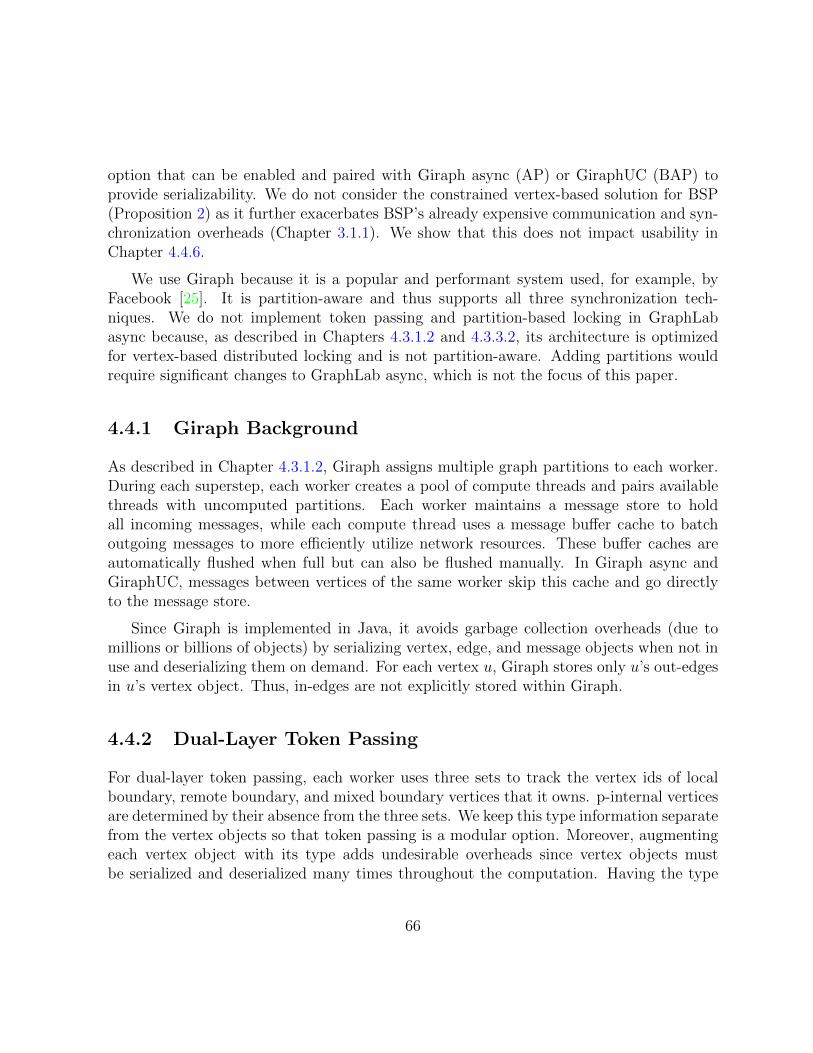
option that can be enabled and paired with Giraph async (AP) or GiraphUC (BAP) toprovide serializability. We do not consider the constrained vertex-based solution for BSP(Proposition 2) as it further exacerbates BSP’s already expensive communication and syn-chronization overheads (Chapter 3.1.1). We show that this does not impact usability inChapter 4.4.6.
We use Giraph because it is a popular and performant system used, for example, byFacebook [25]. It is partition-aware and thus supports all three synchronization tech-niques. We do not implement token passing and partition-based locking in GraphLabasync because, as described in Chapters 4.3.1.2 and 4.3.3.2, its architecture is optimizedfor vertex-based distributed locking and is not partition-aware. Adding partitions wouldrequire significant changes to GraphLab async, which is not the focus of this paper.
4.4.1 Giraph Background
As described in Chapter 4.3.1.2, Giraph assigns multiple graph partitions to each worker.During each superstep, each worker creates a pool of compute threads and pairs availablethreads with uncomputed partitions. Each worker maintains a message store to holdall incoming messages, while each compute thread uses a message buffer cache to batchoutgoing messages to more efficiently utilize network resources. These buffer caches areautomatically flushed when full but can also be flushed manually. In Giraph async andGiraphUC, messages between vertices of the same worker skip this cache and go directlyto the message store.
Since Giraph is implemented in Java, it avoids garbage collection overheads (due tomillions or billions of objects) by serializing vertex, edge, and message objects when not inuse and deserializing them on demand. For each vertex u, Giraph stores only u’s out-edgesin u’s vertex object. Thus, in-edges are not explicitly stored within Giraph.
4.4.2 Dual-Layer Token Passing
For dual-layer token passing, each worker uses three sets to track the vertex ids of localboundary, remote boundary, and mixed boundary vertices that it owns. p-internal verticesare determined by their absence from the three sets. We keep this type information separatefrom the vertex objects so that token passing is a modular option. Moreover, augmentingeach vertex object with its type adds undesirable overheads since vertex objects mustbe serialized and deserialized many times throughout the computation. Having the type
66
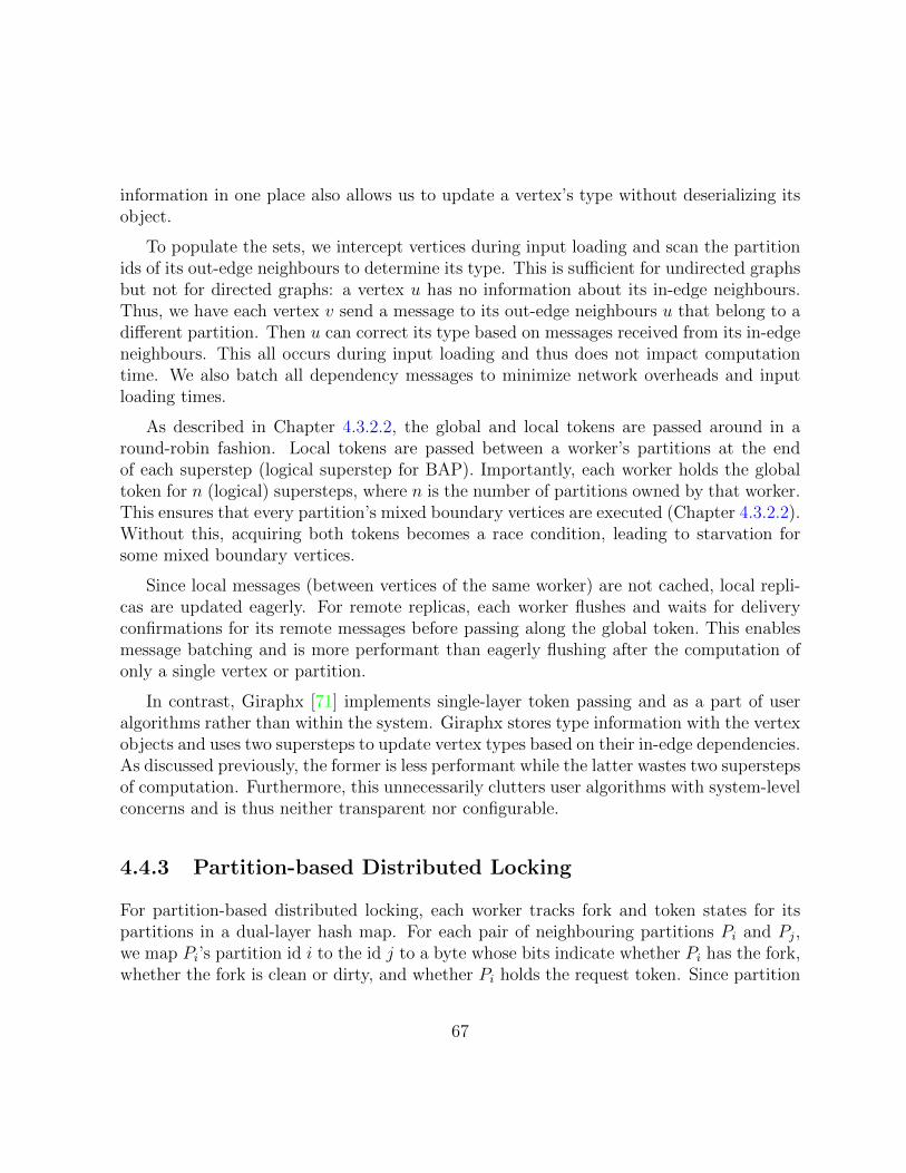
information in one place also allows us to update a vertex’s type without deserializing itsobject.
To populate the sets, we intercept vertices during input loading and scan the partitionids of its out-edge neighbours to determine its type. This is sufficient for undirected graphsbut not for directed graphs: a vertex u has no information about its in-edge neighbours.Thus, we have each vertex v send a message to its out-edge neighbours u that belong to adifferent partition. Then u can correct its type based on messages received from its in-edgeneighbours. This all occurs during input loading and thus does not impact computationtime. We also batch all dependency messages to minimize network overheads and inputloading times.
As described in Chapter 4.3.2.2, the global and local tokens are passed around in around-robin fashion. Local tokens are passed between a worker’s partitions at the endof each superstep (logical superstep for BAP). Importantly, each worker holds the globaltoken for n (logical) supersteps, where n is the number of partitions owned by that worker.This ensures that every partition’s mixed boundary vertices are executed (Chapter 4.3.2.2).Without this, acquiring both tokens becomes a race condition, leading to starvation forsome mixed boundary vertices.
Since local messages (between vertices of the same worker) are not cached, local repli-cas are updated eagerly. For remote replicas, each worker flushes and waits for deliveryconfirmations for its remote messages before passing along the global token. This enablesmessage batching and is more performant than eagerly flushing after the computation ofonly a single vertex or partition.
In contrast, Giraphx [71] implements single-layer token passing and as a part of useralgorithms rather than within the system. Giraphx stores type information with the vertexobjects and uses two supersteps to update vertex types based on their in-edge dependencies.As discussed previously, the former is less performant while the latter wastes two superstepsof computation. Furthermore, this unnecessarily clutters user algorithms with system-levelconcerns and is thus neither transparent nor configurable.
4.4.3 Partition-based Distributed Locking
For partition-based distributed locking, each worker tracks fork and token states for itspartitions in a dual-layer hash map. For each pair of neighbouring partitions Pi and Pj,we map Pi’s partition id i to the id j to a byte whose bits indicate whether Pi has the fork,whether the fork is clean or dirty, and whether Pi holds the request token. Since partition
67
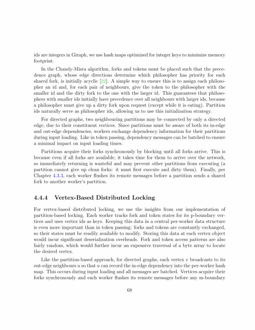
ids are integers in Giraph, we use hash maps optimized for integer keys to minimize memoryfootprint.
In the Chandy-Misra algorithm, forks and tokens must be placed such that the prece-dence graph, whose edge directions determine which philosopher has priority for eachshared fork, is initially acyclic [22]. A simple way to ensure this is to assign each philoso-pher an id and, for each pair of neighbours, give the token to the philosopher with thesmaller id and the dirty fork to the one with the larger id. This guarantees that philoso-phers with smaller ids initially have precedence over all neighbours with larger ids, becausea philosopher must give up a dirty fork upon request (except while it is eating). Partitionids naturally serve as philosopher ids, allowing us to use this initialization strategy.
For directed graphs, two neighbouring partitions may be connected by only a directededge, due to their constituent vertices. Since partitions must be aware of both its in-edgeand out-edge dependencies, workers exchange dependency information for their partitionsduring input loading. Like in token passing, dependency messages can be batched to ensurea minimal impact on input loading times.
Partitions acquire their forks synchronously by blocking until all forks arrive. This isbecause even if all forks are available, it takes time for them to arrive over the network,so immediately returning is wasteful and may prevent other partitions from executing (apartition cannot give up clean forks: it must first execute and dirty them). Finally, perChapter 4.3.3, each worker flushes its remote messages before a partition sends a sharedfork to another worker’s partition.
4.4.4 Vertex-Based Distributed Locking
For vertex-based distributed locking, we use the insights from our implementation ofpartition-based locking. Each worker tracks fork and token states for its p-boundary ver-tices and uses vertex ids as keys. Keeping this data in a central per-worker data structureis even more important than in token passing: forks and tokens are constantly exchanged,so their states must be readily available to modify. Storing this data at each vertex objectwould incur significant deserialization overheads. Fork and token access patterns are alsofairly random, which would further incur an expensive traversal of a byte array to locatethe desired vertex.
Like the partition-based approach, for directed graphs, each vertex v broadcasts to itsout-edge neighbours u so that u can record the in-edge dependency into the per-worker hashmap. This occurs during input loading and all messages are batched. Vertices acquire theirforks synchronously and each worker flushes its remote messages before any m-boundary
68
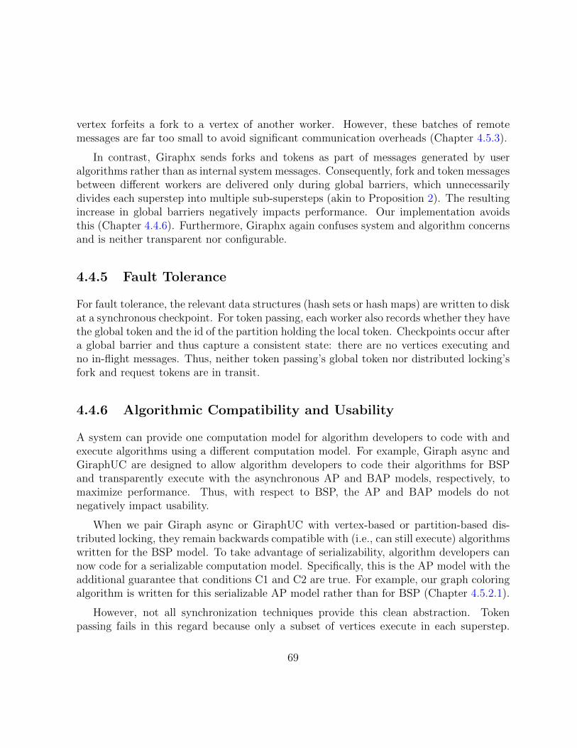
vertex forfeits a fork to a vertex of another worker. However, these batches of remotemessages are far too small to avoid significant communication overheads (Chapter 4.5.3).
In contrast, Giraphx sends forks and tokens as part of messages generated by useralgorithms rather than as internal system messages. Consequently, fork and token messagesbetween different workers are delivered only during global barriers, which unnecessarilydivides each superstep into multiple sub-supersteps (akin to Proposition 2). The resultingincrease in global barriers negatively impacts performance. Our implementation avoidsthis (Chapter 4.4.6). Furthermore, Giraphx again confuses system and algorithm concernsand is neither transparent nor configurable.
4.4.5 Fault Tolerance
For fault tolerance, the relevant data structures (hash sets or hash maps) are written to diskat a synchronous checkpoint. For token passing, each worker also records whether they havethe global token and the id of the partition holding the local token. Checkpoints occur aftera global barrier and thus capture a consistent state: there are no vertices executing andno in-flight messages. Thus, neither token passing’s global token nor distributed locking’sfork and request tokens are in transit.
4.4.6 Algorithmic Compatibility and Usability
A system can provide one computation model for algorithm developers to code with andexecute algorithms using a different computation model. For example, Giraph async andGiraphUC are designed to allow algorithm developers to code their algorithms for BSPand transparently execute with the asynchronous AP and BAP models, respectively, tomaximize performance. Thus, with respect to BSP, the AP and BAP models do notnegatively impact usability.
When we pair Giraph async or GiraphUC with vertex-based or partition-based dis-tributed locking, they remain backwards compatible with (i.e., can still execute) algorithmswritten for the BSP model. To take advantage of serializability, algorithm developers cannow code for a serializable computation model. Specifically, this is the AP model with theadditional guarantee that conditions C1 and C2 are true. For example, our graph coloringalgorithm is written for this serializable AP model rather than for BSP (Chapter 4.5.2.1).
However, not all synchronization techniques provide this clean abstraction. Tokenpassing fails in this regard because only a subset of vertices execute in each superstep.
69
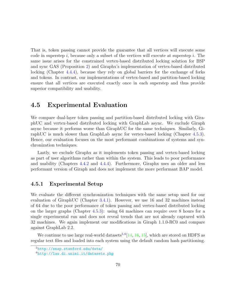
That is, token passing cannot provide the guarantee that all vertices will execute somecode in superstep i, because only a subset of the vertices will execute at superstep i. Thesame issue arises for the constrained vertex-based distributed locking solution for BSPand sync GAS (Proposition 2) and Giraphx’s implementation of vertex-based distributedlocking (Chapter 4.4.4), because they rely on global barriers for the exchange of forksand tokens. In contrast, our implementations of vertex-based and partition-based lockingensure that all vertices are executed exactly once in each superstep and thus providesuperior compatibility and usability.
4.5 Experimental Evaluation
We compare dual-layer token passing and partition-based distributed locking with Gira-phUC and vertex-based distributed locking with GraphLab async. We exclude Giraphasync because it performs worse than GiraphUC for the same techniques. Similarly, Gi-raphUC is much slower than GraphLab async for vertex-based locking (Chapter 4.5.3).Hence, our evaluation focuses on the most performant combinations of systems and syn-chronization techniques.
Lastly, we exclude Giraphx as it implements token passing and vertex-based lockingas part of user algorithms rather than within the system. This leads to poor performanceand usability (Chapters 4.4.2 and 4.4.4). Furthermore, Giraphx uses an older and lessperformant version of Giraph and does not implement the more performant BAP model.
4.5.1 Experimental Setup
We evaluate the different synchronization techniques with the same setup used for ourevaluation of GiraphUC (Chapter 3.4.1). However, we use 16 and 32 machines insteadof 64 due to the poor performance of token passing and vertex-based distributed lockingon the larger graphs (Chapter 4.5.3): using 64 machines can require over 8 hours for asingle experimental run and does not reveal trends that are not already captured with32 machines. We again implement our modifications in Giraph 1.1.0-RC0 and compareagainst GraphLab 2.2.
We continue to use large real-world datasets5,6[14, 16, 15], which are stored on HDFS asregular text files and loaded into each system using the default random hash partitioning.
5http://snap.stanford.edu/data/6http://law.di.unimi.it/datasets.php
70
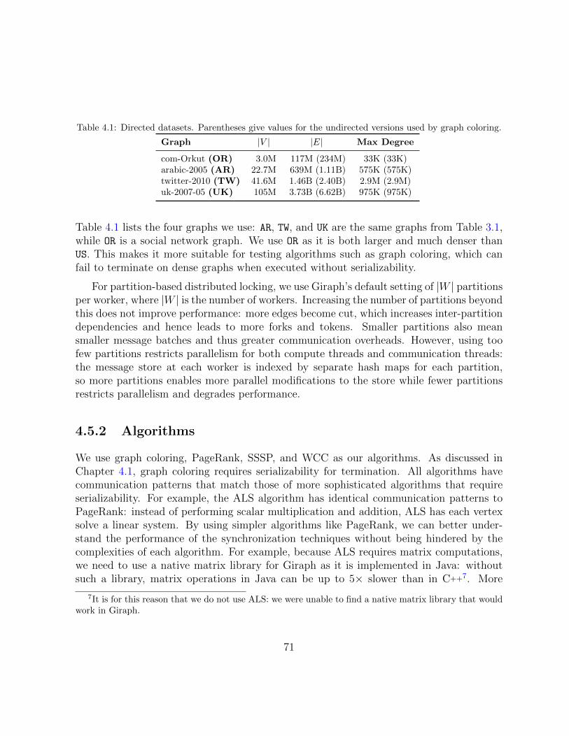
Table 4.1: Directed datasets. Parentheses give values for the undirected versions used by graph coloring.
Graph |V | |E| Max Degree
com-Orkut (OR) 3.0M 117M (234M) 33K (33K)arabic-2005 (AR) 22.7M 639M (1.11B) 575K (575K)twitter-2010 (TW) 41.6M 1.46B (2.40B) 2.9M (2.9M)uk-2007-05 (UK) 105M 3.73B (6.62B) 975K (975K)
Table 4.1 lists the four graphs we use: AR, TW, and UK are the same graphs from Table 3.1,while OR is a social network graph. We use OR as it is both larger and much denser thanUS. This makes it more suitable for testing algorithms such as graph coloring, which canfail to terminate on dense graphs when executed without serializability.
For partition-based distributed locking, we use Giraph’s default setting of |W | partitionsper worker, where |W | is the number of workers. Increasing the number of partitions beyondthis does not improve performance: more edges become cut, which increases inter-partitiondependencies and hence leads to more forks and tokens. Smaller partitions also meansmaller message batches and thus greater communication overheads. However, using toofew partitions restricts parallelism for both compute threads and communication threads:the message store at each worker is indexed by separate hash maps for each partition,so more partitions enables more parallel modifications to the store while fewer partitionsrestricts parallelism and degrades performance.
4.5.2 Algorithms
We use graph coloring, PageRank, SSSP, and WCC as our algorithms. As discussed inChapter 4.1, graph coloring requires serializability for termination. All algorithms havecommunication patterns that match those of more sophisticated algorithms that requireserializability. For example, the ALS algorithm has identical communication patterns toPageRank: instead of performing scalar multiplication and addition, ALS has each vertexsolve a linear system. By using simpler algorithms like PageRank, we can better under-stand the performance of the synchronization techniques without being hindered by thecomplexities of each algorithm. For example, because ALS requires matrix computations,we need to use a native matrix library for Giraph as it is implemented in Java: withoutsuch a library, matrix operations in Java can be up to 5× slower than in C++7. More
7It is for this reason that we do not use ALS: we were unable to find a native matrix library that wouldwork in Giraph.
71
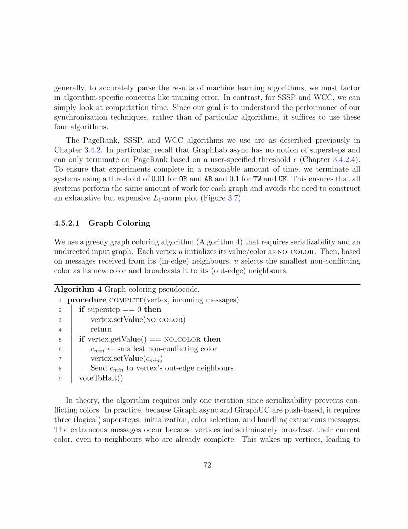
generally, to accurately parse the results of machine learning algorithms, we must factorin algorithm-specific concerns like training error. In contrast, for SSSP and WCC, we cansimply look at computation time. Since our goal is to understand the performance of oursynchronization techniques, rather than of particular algorithms, it suffices to use thesefour algorithms.
The PageRank, SSSP, and WCC algorithms we use are as described previously inChapter 3.4.2. In particular, recall that GraphLab async has no notion of supersteps andcan only terminate on PageRank based on a user-specified threshold ε (Chapter 3.4.2.4).To ensure that experiments complete in a reasonable amount of time, we terminate allsystems using a threshold of 0.01 for OR and AR and 0.1 for TW and UK. This ensures that allsystems perform the same amount of work for each graph and avoids the need to constructan exhaustive but expensive L1-norm plot (Figure 3.7).
4.5.2.1 Graph Coloring
We use a greedy graph coloring algorithm (Algorithm 4) that requires serializability and anundirected input graph. Each vertex u initializes its value/color as no color. Then, basedon messages received from its (in-edge) neighbours, u selects the smallest non-conflictingcolor as its new color and broadcasts it to its (out-edge) neighbours.
Algorithm 4 Graph coloring pseudocode.
1 procedure compute(vertex, incoming messages)2 if superstep == 0 then3 vertex.setValue(no color)4 return
5 if vertex.getValue() == no color then6 cmin ← smallest non-conflicting color7 vertex.setValue(cmin)8 Send cmin to vertex’s out-edge neighbours
9 voteToHalt()
In theory, the algorithm requires only one iteration since serializability prevents con-flicting colors. In practice, because Giraph async and GiraphUC are push-based, it requiresthree (logical) supersteps: initialization, color selection, and handling extraneous messages.The extraneous messages occur because vertices indiscriminately broadcast their currentcolor, even to neighbours who are already complete. This wakes up vertices, leading to
72
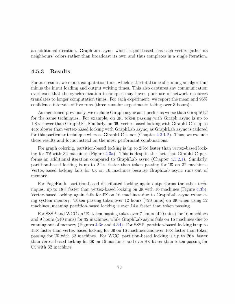
an additional iteration. GraphLab async, which is pull-based, has each vertex gather itsneighbours’ colors rather than broadcast its own and thus completes in a single iteration.
4.5.3 Results
For our results, we report computation time, which is the total time of running an algorithmminus the input loading and output writing times. This also captures any communicationoverheads that the synchronization techniques may have: poor use of network resourcestranslates to longer computation times. For each experiment, we report the mean and 95%confidence intervals of five runs (three runs for experiments taking over 3 hours).
As mentioned previously, we exclude Giraph async as it performs worse than GiraphUCfor the same techniques. For example, on OR, token passing with Giraph async is up to1.8× slower than GiraphUC. Similarly, on OR, vertex-based locking with GiraphUC is up to44× slower than vertex-based locking with GraphLab async, as GraphLab async is tailoredfor this particular technique whereas GiraphUC is not (Chapter 4.3.1.2). Thus, we excludethese results and focus instead on the most performant combinations.
For graph coloring, partition-based locking is up to 2.3× faster than vertex-based lock-ing for TW with 32 machines (Figure 4.3a). This is despite the fact that GiraphUC per-forms an additional iteration compared to GraphLab async (Chapter 4.5.2.1). Similarly,partition-based locking is up to 2.2× faster than token passing for UK on 32 machines.Vertex-based locking fails for UK on 16 machines because GraphLab async runs out ofmemory.
For PageRank, partition-based distributed locking again outperforms the other tech-niques: up to 18× faster than vertex-based locking on OR with 16 machines (Figure 4.3b).Vertex-based locking again fails for UK on 16 machines due to GraphLab async exhaust-ing system memory. Token passing takes over 12 hours (720 mins) on UK when using 32machines, meaning partition-based locking is over 14× faster than token passing.
For SSSP and WCC on UK, token passing takes over 7 hours (420 mins) for 16 machinesand 9 hours (540 mins) for 32 machines, while GraphLab async fails on 16 machines due torunning out of memory (Figures 4.3c and 4.3d). For SSSP, partition-based locking is up to13× faster than vertex-based locking for OR on 16 machines and over 10× faster than tokenpassing for UK with 32 machines. For WCC, partition-based locking is up to 26× fasterthan vertex-based locking for OR on 16 machines and over 8× faster than token passing forUK with 32 machines.
73
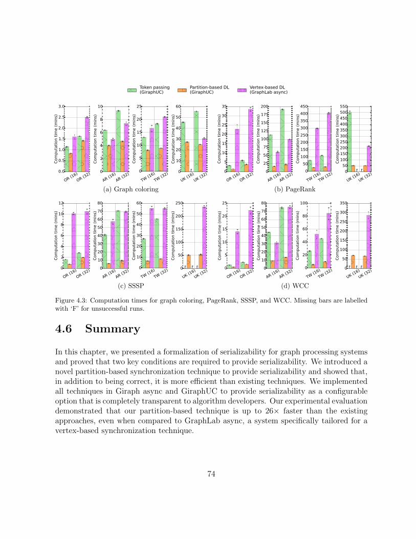
Token passing(GiraphUC)
Partition-based DL(GiraphUC)
Vertex-based DL(GraphLab async)
OR (1
6)
OR (3
2)0.0
0.5
1.0
1.5
2.0
2.5
3.0
Computation tim
e (mins)
AR (16)
AR (32)
0
2
4
6
8
10
Computation tim
e (mins)
TW (16)
TW (32)
0
5
10
15
20
25
Computation tim
e (mins)
UK (16)
UK (32)
0
10
20
30
40
50
60
Computation tim
e (mins)
F
(a) Graph coloring
OR (16)
OR (32)
0
5
10
15
20
25
30
35
Computation tim
e (mins)
AR (16)
AR (32)
0
25
50
75
100
125
150
175
200
Computation tim
e (mins)
TW (16)
TW (32)
0
50
100
150
200
250
300
350
400
450
Computation tim
e (mins)
UK (16)
UK (32)
0
50
100
150
200
250
300
350
400
450
500
550
Computation tim
e (mins)
FF
(b) PageRank
OR (16)
OR (32)
0
2
4
6
8
10
12
Computation tim
e (mins)
AR (16)
AR (32)
0
10
20
30
40
50
60
70
80
Computation tim
e (mins)
TW (16)
TW (32)
0
10
20
30
40
50
60
Computation tim
e (mins)
UK (16)
UK (32)
0
50
100
150
200
250
Computation tim
e (mins)
F FF
(c) SSSP
OR (16)
OR (32)
0
5
10
15
20
25
Computation tim
e (mins)
AR (16)
AR (32)
0
10
20
30
40
50
60
70
80
Computation tim
e (mins)
TW (16)
TW (32)
0
20
40
60
80
100
Computation tim
e (mins)
UK (16)
UK (32)
0
50
100
150
200
250
300
350
Computation tim
e (mins)
F FF
(d) WCC
Figure 4.3: Computation times for graph coloring, PageRank, SSSP, and WCC. Missing bars are labelledwith ‘F’ for unsuccessful runs.
4.6 Summary
In this chapter, we presented a formalization of serializability for graph processing systemsand proved that two key conditions are required to provide serializability. We introduced anovel partition-based synchronization technique to provide serializability and showed that,in addition to being correct, it is more efficient than existing techniques. We implementedall techniques in Giraph async and GiraphUC to provide serializability as a configurableoption that is completely transparent to algorithm developers. Our experimental evaluationdemonstrated that our partition-based technique is up to 26× faster than the existingapproaches, even when compared to GraphLab async, a system specifically tailored for avertex-based synchronization technique.
74
Chapter 5
Conclusion
We began by introducing two major problems of existing specialized Pregel-like graphprocessing systems: (1) poor performance due to frequent global synchronization barriersand (2) a lack of serializability guarantees for graph algorithms. Before addressing thesetwo problems, we first categorized existing Pregel-like systems in Chapter 2, in part toillustrate that solutions to these two problems either do not exist or are inadequate. Wealso characterized several other related systems in the field of graph processing, to showboth how the field has evolved and the future directions in which it may be heading.
In Chapter 3, we addressed problem (1) by introducing a new barrierless asynchronousparallel (BAP) computation model that uses the notions of local barriers and logical super-steps to reduce the frequency of global barriers while maintaining correctness for algorithmswritten for BSP. Consequently, this allows a system to provide algorithm developers witha BSP interface while transparently executing using the asynchronous BAP model to max-imize performance. Our implementation of the BAP model, GiraphUC, demonstratedacross-the-board performance gains of up to 5× faster than Giraph, Giraph async, andGraphLab sync and 86× faster than GraphLab async.
In Chapter 4, we addressed problem (2) by formalizing the notion of serializabilityfor Pregel-like systems and proving that systems can provide serializability when pairedwith a synchronization technique that satisfies two key conditions. We then described andcharacterized the performance of existing synchronization techniques (token passing andvertex-based distributed locking) and introduced a new and more performant partition-based distributed locking technique. Our implementations of these techniques in Giraphasync and GiraphUC demonstrated that our partition-based distributed locking techniqueoutperforms existing techniques by up to 26×, even when compared to GraphLab async,
75
a system tailored for the vertex-based distributed locking technique.
5.1 Future Work
There remains several interesting research questions for both GiraphUC and serializability.Specifically, how to provide support for aggregators that require global coordination inGiraphUC (Chapter 5.1.1) and how to generalize serializability to algorithms where verticescan communicate with arbitrary vertices (Chapter 5.1.2). We also pose broader long-termquestions in Chapter 5.1.3 regarding the integration of BAP and serializability into genericbig data systems.
5.1.1 Globally Coordinated Aggregators
In BSP, algorithms use aggregators to record global information: for example, the numberof vertices that successfully completed some task in the previous superstep. Each vertexcan contribute a value to an aggregator in superstep i and that aggregator’s value is madeavailable to all vertices in superstep i + 1. However, in many cases, algorithms requireonly per-worker information for correctness. That is, they do not require aggregatorsthat are globally coordinated: instead of each vertex needing to see an aggregated valueaccumulated from all vertices of all workers in a previous superstep, a vertex of workerWj needs to see only the aggregated value accumulated from Wj’s vertices in the previouslogical superstep.
GiraphUC supports aggregators that do not need to be globally coordinated since, inpractice, few algorithms require globally coordinated aggregators. For example, in Table2.1, only K-means requires globally coordinated aggregators. Additionally, since GiraphUCsupports multi-phase algorithms, it naturally supports globally coordinated aggregatorsused for denoting which computation phase the algorithm is in. However, GiraphUC doesnot efficiently support other forms of globally coordinated aggregators: ensuring that theaggregator’s value is always correct requires all workers to wait for each other, which meansthere must be frequent global barriers and so BAP effectively degrades to AP.
Thus, an open question is whether it is possible to support globally coordinated ag-gregators in a more efficient manner, while maintaining correctness under the BSP model.For example, instead of synchronizing all workers with a global barrier, can we have fasterworkers use stale aggregator values in lieu of receiving newer values from their slower neigh-bours (similar to Theorem 2)? Or, alternatively, can globally coordinated aggregators be
76
converted into equivalent per-worker aggregators? In the latter case, the BSP interface canbe modified slightly, as done for multi-phase algorithms (Chapter 3.2.3), to allow algorithmdevelopers to specify these per-worker aggregators.
5.1.2 Generalized Serializability
In Chapter 4, we formalized serializability for algorithms where vertices communicate onlywith their direct neighbours. This covers many machine learning and graph analytic al-gorithms that require serializability. In fact, we were unable to find any examples ofalgorithms that required both serializability and communication with arbitrary vertices.
Nevertheless, it would be useful to generalize serializability support to include algo-rithms that communicate with arbitrary vertices. Supporting this within the graph pro-cessing system is much more challenging as the read set of each transaction is no longerknown a priori (Chapter 4.2.2), meaning condition C2 of Theorem 4 is insufficient forguaranteeing non-conflicting operations. That is, the read set of each vertex is, in general,determined dynamically at runtime.
One possible solution is to provide an API that, for each vertex u, enables the algorithmdeveloper to instruct the system on which vertices u must be coordinated with prior tou being executed. However, this may not always be possible if, for example, within asingle superstep, each vertex u sends messages to vertices whose ids are given by thereceived messages that u must first read. To get around this, one might further modifythe interface to separate message reading from the compute function. However, such asolution will negatively impact usability and compatibility.
A more general solution is to introduce the notion of an abort, to allow for transactionsto be cancelled and rolled back. However, this requires a significant and non-trivial redesignof the graph processing system to make it transaction-aware: it must track and explicitlycommit or abort all transactions. In contrast, the synchronization techniques we introducedin Chapter 4.3 do not require the system to be transaction-aware: the techniques simply runon top of the existing system. A redesign is necessary to support aborts because systemsthat are not transaction-aware will suffer cascading aborts: messages will be erroneouslysent before a commit occurs and there is no simple way to undo a message once it is sent.In the worst case, such a scenario would require rolling back the entire graph state.
77
5.1.3 Asynchronous Models in Generic Systems
There is now a greater focus on providing graph analytics on generic big data systems suchas dataflow engines, like Spark [82] and Hyracks [18], and relational databases (Chapter2.4). Unlike specialized graph processing systems, where there is a direct mapping fromgraph analytics to the internal system implementation, graph analytics built on genericbig data systems are abstracted away from the underlying system implementation. Forexample, dataflow engines simulate graph operations by performing joins on tables whilerelational databases translate graph operations to relational operations.
Thus, a more general open question is whether asynchronous models, such as BAP, canbe implemented on these generic big data systems to provide performance gains despitethe extra layer of abstraction. Alternatively, can the notions of local barriers and logicalsupersteps be translated into mechanisms that affect the implementation of generic bigdata systems to enhance their graph analytics performance?
Similarly, it may be possible to continue to provide serializability in a configurable andtransparent manner by translating the synchronization techniques for use with these genericbig data systems. In particular, relational databases may be a better option for providinggeneralized serializability (Chapter 5.1.2), as they are typically transaction-aware and canthus avoid the non-trivial redesign required by specialized graph processing systems.
78

APPENDICES
79

Appendix A
Proofs for Giraph Unchained
In this chapter, we provide proofs for Theorems 1 and 2 of Chapter 3.
A.1 Preliminaries
Single-phase (BSP) algorithms are so named because they have a single computation phase.That is, the compute function executed by vertices always contains the same logic for everysuperstep. For example, if the compute function contains branching logic based on thesuperstep count or some aggregator value, then it is composed of multiple computationphases1 and therefore not a single-phase algorithm. The exceptions to this are initialization,which is conditional on it being the first superstep, and termination, such as voting tohalt after K supersteps. The former is a special case that we can handle directly in theimplementation, while the latter is termination and so there is no additional logic that willfollow. Specifically, many algorithms perform initialization procedures in the first (logical)superstep and send, but do not receive, messages. This can be handled by keeping allmessages in the message store until the second (logical) superstep. This is correct, sincein BSP no sent messages will be seen by any vertex in the first (logical) superstep.
Since both the AP and BAP models execute only algorithms implemented for the BSPmodel, we need only consider single-phase BSP algorithms. From the discussion above,such algorithms have the following property:
1Theorem 3 describes how the AP and BAP models handle multi-phase algorithms.
80
Property I: The computation logic for single-phase BSP algorithms is the same for everysuperstep.
Secondly, because of the iterative nature of BSP, a message m sent by an arbitraryvertex v is either a function of v’s vertex value or it is not. That is, an algorithm eitherhas all messages of the form m = f(vvalue), where v is the sender of m, or all messagesof the form m 6= f(vvalue). All messages of any particular algorithm are always of oneform because, by Property I, the computation logic generating the messages is always thesame. In the first case, v’s vertex value is a function of v’s previous vertex values, so mencapsulates v’s most recent vertex value as well as all past values, meaning that newermessages contain more information than older messages. Then, since newer messages aremore important than older messages, each vertex needs to see only the newest messagessent to it. In the second case, the algorithm is an accumulative update algorithm [85]where old messages are as important as new messages, because m does not encapsulate v’sprevious values. Hence, each vertex must see all messages sent to it exactly once. Thenwe have the following two properties:
Property II: For an algorithm with messages m = f(vvalue), where m is sent by a vertexv, a new message from v to a vertex u is more important than an old message from v to uand so u must see the newest message sent to it by v.
Property III: For an algorithm with messages m 6= f(vvalue), where m is sent by a vertexv, all messages from v to a vertex u are important and so u must see all messages sent toit by v exactly once.
Note that both Properties II and III are enforced in the BSP model since implemen-tations ensure that messages are delivered exactly once and not lost, by acknowledgingdelivery of messages and retrying failed sends. Since message stores buffer all receivedmessages exactly once and remove all the messages for a vertex u when computing u, thevertex u will see all messages sent to it exactly once.
All single-phase BSP algorithms can be defined as one of two types: ones in whichvertices do not need all messages from all neighbours (type A) and ones in which verticesneed all messages from all neighbours (type B). Since accumulative update algorithms arealways type A algorithms [85], messages of type A algorithms are either all of the formm = f(vvalue) or all of the form m 6= f(vvalue), while messages of type B algorithms arealways of the form m = f(vvalue).
81
A.1.1 Type A
Type A algorithms satisfy both Properties II and III above, as it must handle messages ofboth forms. Since Property III is more restrictive (that is, it being true implies PropertyII is also true), the invariant for type A algorithms is simply Property III:
Invariant A: All messages sent from a vertex v to a vertex u must be seen by u exactlyonce.
Furthermore, the definition of type A algorithms places no constraints on when a ver-tex’s neighbours are active or inactive. That is, a vertex’s neighbours can become activeor inactive at any superstep during the computation. Consequently, its compute functioncan receive any number of messages in each superstep, which means it must be capable ofprocessing such messages (otherwise, the algorithm would not be correct even for BSP):
Property A: The compute function of type A algorithms correctly handles any numberof messages in each superstep.
A.1.2 Type B
Unlike type A algorithms, type B algorithms have only one form of messages so it satisfiesonly Property II. However, since the definition of a type B algorithm is more restrictivethan Property II, its invariant follows directly from its definition:
Invariant B: Each vertex must see exactly one message from each of its in-edge neighboursat every superstep.
For type B algorithms, a vertex’s neighbours are always active since each vertex mustreceive messages from all their neighbours. Intuitively, if even one vertex is inactive, itwill stop sending messages to its neighbours and thus violate the definition of type Balgorithms. Since all messages for type B algorithms are of the form m = f(vvalue), then byProperty II, not every message from a vertex v to another vertex u is important becausewe will always see a newer message from v (unless the algorithm is terminating, but in thatcase u would be halting as well). That is, correctness is still maintained when a vertex usees only a newer message m′ sent to it by v and not any older messages m from v, sincem′ is more important than m. Therefore:
Property B: An old message m from vertex v to u can be overwritten by a new messagem′ from v to u.
82
Note that, unlike type A algorithms, the compute function of type B algorithms canonly correctly process N messages when executing on a vertex u with N in-edge neighbours.Processing fewer or more messages will cause vertex u to have an incorrect vertex value.Invariant B ensures that this constraint on the computation logic is satisfied.
A.2 Theorem 1
Theorem 1. The AP and BAP models correctly execute single-phase BSP algorithms inwhich vertices do not need all messages from all neighbours.
Proof. As mentioned in Appendix A.1 above, we need only focus on the type A algorithms.Specifically, we must show that (1) relaxing message isolation and, for BAP, removingglobal barriers does not impact the algorithm’s correctness and (2) Invariant A is enforcedby both models.
For (1), relaxing message isolation means that messages are seen earlier than they wouldhave been seen in the BSP model, while the removal of global barriers means a messagefrom any superstep can arrive at any time.
By Property I, a received message will be processed in the same way in the current su-perstep as it would in any other superstep, because the computation logic is the same in allsupersteps. Thus, showing messages from different supersteps does not affect correctness,meaning that relaxing message isolation does not impact correctness.
By Property A, vertices can process any number of received messages. That is, cor-rectness is maintained even if messages are delayed2 and hence not passed to the vertex’scompute function or a large number of messages suddenly arrive and are all passed tothe vertex’s compute function. Together with Property I, this shows that removing globalbarriers does not impact correctness.
For (2), like BSP, the message stores of both the AP and BAP models still buffer allreceived messages by default and, when computing a vertex u, will remove all messagesfor u from the message store (Chapter 3.3.2). Since the implementations of both modelsensure messages are delivered exactly once and are not lost, we can ensure that the messagestore buffers all messages for u exactly once and thus u sees all messages from senders vexactly once. More precisely, the AP and BAP models still guarantee message delivery like
2At the implementation level, messages are guaranteed to be delivered, so a message may be delayedbut is never lost.
83
the BSP model—the models modify when a message is received, not whether a messagewill be delivered. This is enforced in the implementation in the same way as it is forimplementations of the BSP model: by using acknowledgements and resending messagesthat fail to deliver.
A.3 Theorem 2
Theorem 2. Given a message store that is initially filled with valid messages, retains oldmessages, and overwrites old messages with new messages, the BAP model correctly exe-cutes single-phase BSP algorithms in which vertices need all messages from all neighbours.
Proof. As mentioned in Appendix A.1, we need only focus on the type B algorithms.Specifically, we must show that (1) relaxing message isolation and removing global barriersdoes not impact the algorithm’s correctness and (2) Invariant B is maintained by the BAPmodel. Note that proving Theorem 2 for the BAP model also proves it for the AP modelsince BAP subsumes AP.
First, note that the theorem states three assumptions about the message store: it isinitially filled with valid messages, it retains old messages (i.e., does not remove them),and new messages overwrite old messages. More concretely, consider an arbitrary vertex uwith neighbours vi, 0 ≤ i < N , where N = deg−(u) is the number of in-edges (or in-edgeneighbours) of u. Then, initially, the message store will have exactly one message mi fromeach of u’s neighbours vi. That is, when computing u, the system will pass the set ofmessages S = {mi}∀i, with |S| = N , to u’s compute function. If u is to be computedagain and no new messages have arrived, the message store retains all the old messagesand so S = {mi}∀i is simply passed to u’s compute function again. If a new message m′jarrives from one of u’s neighbours vj, j ∈ [0, N), it will overwrite the old message mj. FromProperty B, performing message overwrites in this way will not affect correctness. Then theset of messages passed to u’s compute function will now be S = {mi}∀i∪{m′j}\{mj}, whereagain we preserve |S| = N and exactly one message from each of u’s in-edge neighbours.
Then by the above, the BAP model maintains Invariant B: on every logical superstep,the message store passes to u exactly one message from each of its in-edge neighbours.Hence, (2) is true. For (1), relaxing message isolation does not affect correctness since, byProperty I, received messages are processed in the same way in every superstep and, since(2) is true, we already satisfy Invariant B. Removing global barriers also does not affectcorrectness since messages can be delayed or arrive in large numbers without affecting thenumber or source of messages in the message store: old messages are retained if messages
84

are delayed, while newly arrived messages overwrite existing ones. Thus, the message storewill still have exactly one message from each of u’s in-edge neighbours.
85
References
[1] Apache Giraph. http://giraph.apache.org.
[2] Apache Hadoop. http://hadoop.apache.org.
[3] Apache Hama. http://hama.apache.org.
[4] Neo4j. http://www.neo4j.com.
[5] Okapi. http://grafos.ml/okapi.
[6] OrientDB. http://www.orientdb.com.
[7] Titan. http://thinkaurelius.github.io/titan/.
[8] GraphLab: Distributed Graph-Parallel API. http://docs.graphlab.org/
classgraphlab_1_1async__consistent__engine.html, 2014.
[9] Lada A. Adamic and Eytan Adar. Friends and neighbors on the web. Social Networks,25(3):211–230, 2003.
[10] Alexander Alexandrov, Rico Bergmann, Stephan Ewen, Johann-Christoph Freytag,Fabian Hueske, Arvid Heise, Odej Kao, Marcus Leich, Ulf Leser, Volker Markl, FelixNaumann, Mathias Peters, Astrid Rheinlnder, Matthias J. Sax, Sebastian Schelter,Mareike Hger, Kostas Tzoumas, and Daniel Warneke. The Stratosphere Platform forBig Data Analytics. The VLDB Journal, 23(6):939–964, 2014.
[11] Lars Backstrom, Paolo Boldi, Marco Rosa, Johan Ugander, and Sebastiano Vigna.Four Degrees of Separation. In WebSci ’12, pages 33–42, 2012.
[12] Nguyen Thien Bao and Toyotaro Suzumura. Towards Highly Scalable Pregel-basedGraph Processing Platform with x10. In WWW ’13 Companion, pages 501–508, 2013.
86
[13] Philip A. Bernstein, Vassos Hadzilacos, and Nathan Goodman. Concurrency Controland Recovery in Database Systems. Addison-Wesley Publishing Company, 1987.
[14] P. Boldi and S. Vigna. The Webgraph Framework I: Compression Techniques. InWWW ’04, pages 595–602, 2004.
[15] Paolo Boldi, Bruno Codenotti, Massimo Santini, and Sebastiano Vigna. Ubi-Crawler: A Scalable Fully Distributed Web Crawler. Software: Practice & Experience,34(8):711–726, 2004.
[16] Paolo Boldi, Marco Rosa, Massimo Santini, and Sebastiano Vigna. Layered LabelPropagation: A MultiResolution Coordinate-Free Ordering for Compressing SocialNetworks. In WWW ’11, pages 587–596, 2011.
[17] Paolo Boldi and Sebastiano Vigna. Four Degrees of Separation, Really. http://
arxiv.org/abs/1205.5509, 2012.
[18] Vinayak R. Borkar, Michael J. Carey, Raman Grover, Nicola Onose, and Rares Ver-nica. Hyracks: A Flexible and Extensible Foundation for Data-Intensive Computing.In ICDE ’11, pages 1151–1162, 2011.
[19] Joseph K. Bradley, Aapo Kyrola, Danny Bickson, and Carlos Guestrin. Parallel Co-ordinate Descent for L1-Regularized Loss Minimization. In ICML, 2011.
[20] Yingyi Bu, Vinayak Borkar, Jianfeng Jia, Michael J. Carey, and Tyson Condie.Pregelix: Big(ger) Graph Analytics on A Dataflow Engine. PVLDB, 8(2):161–172,2015.
[21] Yingyi Bu, Bill Howe, Magdalena Balazinska, and Michael D. Ernst. HaLoop: EfficientIterative Data Processing on Large Clusters. PVLDB, 3(1–2):285–296, 2010.
[22] K. M. Chandy and J. Misra. The Drinking Philosophers Problem. ACM Trans.Program. Lang. Syst., 6(4):632–646, 1984.
[23] Rishan Chen, Xuetian Weng, Bingsheng He, and Mao Yang. Large Graph Processingin the Cloud. In SIGMOD ’10, pages 1123–1126, 2010.
[24] Jiefeng Cheng, Qin Liu, Zhenguo Li, Wei Fan, John C.S. Lui, and Cheng He. VENUS:Vertex-Centric Streamlined Graph Computation on a Single PC. In ICDE ’15, 2015.
[25] Avery Ching. Scaling Apache Giraph to a trillion edges. http://www.facebook.com/10151617006153920, 2013.
87
[26] Sun Chung and Anne Condon. Parallel Implementation of Borvka’s Minimum Span-ning Tree Algorithm. In IPPS ’96, pages 302–308, 1996.
[27] Thomas H. Cormen, Charles E. Leiserson, Ronald L. Rivest, and Clifford Stein. In-troduction to Algorithms. The MIT Press, 3rd edition, 2009.
[28] Gianmarco De Francisci Morales, Aristides Gionis, and Mauro Sozio. Social ContentMatching in MapReduce. Proceedings of the VLDB Endowment, 4(7):460–469, 2011.
[29] Jeffrey Dean and Sanjay Ghemawat. MapReduce: Simplified Data Processing onLarge Clusters. In OSDI ’04, 2004.
[30] Jim Edwards. ‘Facebook Inc.’ Actually Has 2.2 Billion Users Now. http://www.
businessinsider.com/facebook-inc-has-22-billion-users-2014-7, 2014.
[31] Jaliya Ekanayake, Hui Li, Bingjing Zhang, Thilina Gunarathne, Seung-Hee Bae, JudyQiu, and Geoffrey Fox. Twister: A Runtime for Iterative MapReduce. In HPDC ’10,pages 810–818, 2010.
[32] Jing Fan, Adalbert Gerald, Soosai Raj, and Jignesh M. Patel. The Case AgainstSpecialized Graph Analytics Engines. In CIDR ’15, 2015.
[33] Joseph Gonzalez, Yucheng Low, Arthur Gretton, and Carlos Guestrin. Parallel GibbsSampling: From Colored Fields to Thin Junction Trees. In AISTATS, volume 15,pages 324–332, 2011.
[34] Joseph E. Gonzalez, Yucheng Low, Haijie Gu, Danny Bickson, and Carlos Guestrin.PowerGraph: Distributed graph-parallel computation on natural graphs. In OSDI’12, pages 17–30, 2012.
[35] Google. How search works. http://www.google.com/insidesearch/
howsearchworks/thestory/, 2014.
[36] Yong Guo, Marcin Biczak, Ana Lucia Varbanescu, Alexandru Iosup, Claudio Martella,and Theodore L. Willke. How Well do Graph-Processing Platforms Perform? AnEmpirical Performance Evaluation and Analysis. In IPDPS 2014, 2014.
[37] M.N. Gurcan, L.E. Boucheron, A. Can, A. Madabhushi, N.M. Rajpoot, and B. Yener.Histopathological Image Analysis: A Review. IEEE Rev Biomed Eng, 2:147–171,2009.
88
[38] Minyang Han and Khuzaima Daudjee. Giraph Unchained: Barrierless AsynchronousParallel Execution in Pregel-like Graph Processing Systems. PVLDB, 8(9):950–961,2015.
[39] Minyang Han, Khuzaima Daudjee, Khaled Ammar, M. Tamer Ozsu, Xingfang Wang,and Tianqi Jin. An Experimental Comparison of Pregel-like Graph Processing Sys-tems. PVLDB, 7(12):1047–1058, 2014.
[40] Wook-Shin Han, Sangyeon Lee, Kyungyeol Park, Jeong-Hoon Lee, Min-Soo Kim,Jinha Kim, and Hwanjo Yu. TurboGraph: A Fast Parallel Graph Engine HandlingBillion-scale Graphs in a Single PC. In KDD ’13, pages 77–85, 2013.
[41] Imranul Hoque and Indranil Gupta. LFGraph: Simple and Fast Distributed GraphAnalytics. In TRIOS ’13, pages 9:1–9:17, 2013.
[42] Alekh Jindal, Praynaa Rawlani, Eugene Wu, Samuel Madden, Amol Deshpande, andMike Stonebraker. Vertexica: Your Relational Friend for Graph Analytics! PVLDB,7(13):1669–1672, 2014.
[43] U. Kang, Charalampos E. Tsourakakis, Ana Paula Appel, Christos Faloutsos, andJure Leskovec. HADI: Mining Radii of Large Graphs. ACM TKDD, 5(2):8:1–8:24,2011.
[44] U. Kang, Charalampos E. Tsourakakis, and Christos Faloutsos. PEGASUS: A Peta-Scale Graph Mining System Implementation and Observations. In ICDM ’09, pages229–238, 2009.
[45] Zuhair Khayyat, Karim Awara, Amani Alonazi, Hani Jamjoom, Dan Williams, andPanos Kalnis. Mizan: A system for dynamic load balancing in large-scale graphprocessing. In EuroSys ’13, pages 169–182, 2013.
[46] Yehuda Koren. Factorization Meets the Neighborhood: A Multifaceted CollaborativeFiltering Model. In KDD ’08, pages 426–434, 2008.
[47] Yehuda Koren, Robert Bell, and Chris Volinsky. Matrix Factorization Techniques forRecommender Systems. IEEE Computer, 42(8):30–37, 2009.
[48] Aapo Kyrola, Guy Blelloch, and Carlos Guestrin. GraphChi: Large-scale GraphComputation on Just a PC. In OSDI ’12, pages 31–46, 2012.
[49] Ian X. Y. Leung, Pan Hui, Pietro Lio, and Jon Crowcroft. Towards real-time commu-nity detection in large networks. Physical Review E, 79(6):066107, 2009.
89
[50] Yucheng Low, Danny Bickson, Joseph Gonzalez, Carlos Guestrin, Aapo Kyrola, andJoseph M. Hellerstein. Distributed GraphLab: A Framework for Machine Learningand Data Mining in the Cloud. PVLDB, 5(8):716–727, 2012.
[51] Yi Lu, James Cheng, Da Yan, and Huanhuan Wu. Large-scale distributed graph com-puting systems: An experimental evaluation. Proceedings of the VLDB Endowment,8(3), 2014.
[52] Michael Luby. A Simple Parallel Algorithm for the Maximal Independent Set Problem.SIAM Journal on Computing, 15(4):1036–1053, 1986.
[53] Maja Kabiljo. Improve the way we keep outgoing messages. http://issues.apache.org/jira/browse/GIRAPH-388, 2012.
[54] Grzegorz Malewicz, Matthew H. Austern, Aart JC Bik, James C. Dehnert, Ilan Horn,Naty Leiser, and Grzegorz Czajkowski. Pregel: A system for large-scale graph pro-cessing. In SIGMOD/PODS ’10, pages 135–146, 2010.
[55] Robert Ryan McCune, Tim Weninger, and Greg Madey. Thinking Like a Vertex: aSurvey of Vertex-Centric Frameworks for Large-Scale Distributed Graph Processing.2015.
[56] Simona Mihaela Orzan. On Distributed Verification and Verified Distribution. PhDthesis, Free University of Amsterdam, 2004.
[57] Robert Preis. Linear Time 1/2-Approximation Algorithm for Maximum WeightedMatching in General Graphs. In STACS ’99, pages 259–269, 1998.
[58] Natasa Przulj. Protein-protein interactions: Making sense of networks via graph-theoretic modeling. BioEssays, 33(2):115–123, 2011.
[59] Louise Quick, Paul Wilkinson, and David Hardcastle. Using Pregel-like Large ScaleGraph Processing Frameworks for Social Network Analysis. In ASONAM ’12, pages457–463, 2012.
[60] Usha Nandini Raghavan, Reka Albert, and Soundar Kumara. Near linear time al-gorithm to detect community structures in large-scale networks. Physical Review E,76(3):036106, 2007.
[61] Marko A. Rodriguez. Faunus Provides Big GraphData Analytics. http://thinkaurelius.com/2012/11/11/
faunus-provides-big-graph-data-analytics/, 2012.
90
[62] Amitabha Roy, Ivo Mihailovic, and Willy Zwaenepoel. X-Stream: Edge-centric GraphProcessing Using Streaming Partitions. In SOSP ’13, pages 472–488, 2013.
[63] Semih Salihoglu and Jennifer Widom. GPS: A Graph Processing System. In SSDBM’13, pages 22:1–22:12, 2013.
[64] Semih Salihoglu and Jennifer Widom. Optimizing Graph Algorithms on Pregel-likeSystems. Technical report, Stanford, 2013.
[65] Zechao Shang and Jeffrey Xu Yu. Catch the Wind: Graph Workload Balancing onCloud. In ICDE ’13, pages 553–564, 2013.
[66] Bin Shao, Haixun Wang, and Yatao Li. Trinity: A Distributed Graph Engine on aMemory Cloud. In SIGMOD ’13, pages 505–516, 2013.
[67] Athanassios G. Siapas. Criticality and Parallelism in Combinatorial Optimization.PhD thesis, Massachusetts Institute of Technology, 1996.
[68] David Simmen, Karl Schnaitter, Jeff Davis, Yingjie He, Sangeet Lohariwala, AjayMysore, Vinayak Shenoi, Mingfeng Tan, and Yu Xiao. Large-scale Graph Analyticsin Aster 6: Bringing Context to Big Data Discovery. PVLDB, 7(13):1405–1416, 2014.
[69] Philip Stutz, Abraham Bernstein, and William Cohen. Signal/Collect: Graph Algo-rithms for the (Semantic) Web. In ISWC’10, pages 764–780, 2010.
[70] Siddharth Suri and Sergei Vassilvitskii. Counting Triangles and the Curse of the LastReducer. WWW ’11, pages 607–614, 2011.
[71] Serafettin Tasci and Murat Demirbas. Giraphx: Parallel Yet Serializable Large-scaleGraph Processing. In Euro-Par ’13, pages 458–469, 2013.
[72] Yuanyuan Tian, Andrey Balmin, Severin Andreas Corsten, Shirish Tatikonda, andJohn McPherson. From “Think Like a Vertex” to “Think Like a Graph”. PVLDB,7(3):193–204, 2013.
[73] Leslie G. Valiant. A Bridging Model for Parallel Computation. Commun. ACM,33(8):103–111, 1990.
[74] Guozhang Wang, Wenlei Xie, Alan J. Demers, and Johannes Gehrke. Asynchronouslarge-scale graph processing made easy. In CIDR ’13, 2013.
91
[75] Chenning Xie, Rong Chen, Haibing Guan, Binyu Zang, and Haibo Chen. SYNC orASYNC: Time to Fuse for Distributed Graph-parallel Computation. In PPoPP’15,2015.
[76] Wenlei Xie, Guozhang Wang, David Bindel, Alan Demers, and Johannes Gehrke. FastIterative Graph Computation with Block Updates. PVLDB, 6(14):2014–2025, 2013.
[77] Reynold S. Xin, Daniel Crankshaw, Ankur Dave, Joseph E. Gonzalez, Michael J.Franklin, and Ion Stoica. GraphX: Unifying Data-Parallel and Graph-Parallel Ana-lytics. http://arxiv.org/abs/1402.2394, 2014.
[78] Reynold S. Xin, Joseph E. Gonzalez, Michael J. Franklin, and Ion Stoica. GraphX: AResilient Distributed Graph System on Spark. In GRADES ’13, pages 2:1–2:6, 2013.
[79] Jilong Xue, Zhi Yang, Zhi Qu, Shian Hou, and Yafei Dai. Seraph: An Efficient,Low-cost System for Concurrent Graph Processing. In HPDC ’14, pages 227–238,2014.
[80] Da Yan, James Cheng, Yi Lu, and Wilfrend Ng. Blogel: A Block-Centric Frameworkfor Distributed Computation on Real-World Graphs. PVLDB, 7(14):1981–1992, 2014.
[81] Da Yan, James Cheng, Kai Xing, Yi Lu, Wilfred Ng, and Yingyi Bu. Pregel Algorithmsfor Graph Connectivity Problems with Performance Guarantees. Proceedings of theVLDB Endowment, 7(14):1821–1832, 2014.
[82] Matei Zaharia, Mosharaf Chowdhury, Michael J. Franklin, Scott Shenker, and IonStoica. Spark: Cluster Computing with Working Sets. In HotCloud ’10, 2010.
[83] Yanfeng Zhang, Qixin Gao, Lixin Gao, and Cuirong Wang. iMapReduce: A Dis-tributed Computing Framework For Iterative Computation. In DataCloud ’11, pages1112–1121, 2011.
[84] Yanfeng Zhang, Qixin Gao, Lixin Gao, and Cuirong Wang. PrIter: A DistributedFramework for Prioritized Iterative Computations. In SOCC ’11, pages 13:1–13:14,2011.
[85] Yanfeng Zhang, Qixin Gao, Lixin Gao, and Cuirong Wang. Accelerate Large-scale It-erative Computation Through Asynchronous Accumulative Updates. In ScienceCloud’12, pages 13–22, 2012.
92
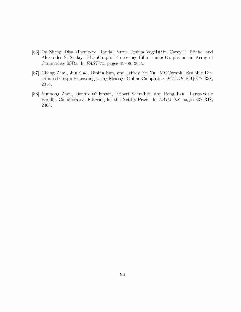
[86] Da Zheng, Disa Mhembere, Randal Burns, Joshua Vogelstein, Carey E. Priebe, andAlexander S. Szalay. FlashGraph: Processing Billion-node Graphs on an Array ofCommodity SSDs. In FAST’15, pages 45–58, 2015.
[87] Chang Zhou, Jun Gao, Binbin Sun, and Jeffrey Xu Yu. MOCgraph: Scalable Dis-tributed Graph Processing Using Message Online Computing. PVLDB, 8(4):377–388,2014.
[88] Yunhong Zhou, Dennis Wilkinson, Robert Schreiber, and Rong Pan. Large-ScaleParallel Collaborative Filtering for the Netflix Prize. In AAIM ’08, pages 337–348,2008.
93