on exponential domination of graphs michael dairyko

On exponential domination of graphs

by

Michael Dairyko

A dissertation submitted to the graduate faculty

in partial fulfillment of the requirements for the degree of

DOCTOR OF PHILOSOPHY

Major: Applied Mathematics

Program of Study Committee:Michael Young, Co-major ProfessorLeslie Hogben, Co-major Professor

Steve ButlerBernard Lidicky

James Rossmanith

The student author, whose presentation of the scholarship herein was approved by the program ofstudy committee, is solely responsible for the content of this dissertation. The Graduate Collegewill ensure this dissertation is globally accessible and will not permit alterations after a degree is

conferred.

Iowa State University

Ames, Iowa

2018

Copyright © Michael Dairyko, 2018. All rights reserved.

ii

DEDICATION

Graduate school is an emotional roller coaster of highs and lows. I would like to take this

opportunity to dedicate this work to the people who supported me during my graduate experience:

To my parents, Greg and Ellen, for their constant support of my endeavors and for being the best

role models I could ever ask for. To my siblings, Gregory and Jenny, for setting the standard of

Dairyko excellence high. To all my friends, old and new, who have shaped me to be the person

that I am, have given me a shoulder to lean on, an ear to listen with, and a smile to laugh to. To

the Posse Foundation and Pomona Posse 5, who started my way down this path and gave me the

drive to become an agent of change.

iii

TABLE OF CONTENTS

Page

LIST OF TABLES . . . . . . . . . . . . . . . . . . . . . . . . . . . . . . . . . . . . . . . . . . v

LIST OF FIGURES . . . . . . . . . . . . . . . . . . . . . . . . . . . . . . . . . . . . . . . . . vi

ACKNOWLEDGEMENTS . . . . . . . . . . . . . . . . . . . . . . . . . . . . . . . . . . . . . viii

ABSTRACT . . . . . . . . . . . . . . . . . . . . . . . . . . . . . . . . . . . . . . . . . . . . . ix

CHAPTER 1. INTRODUCTION . . . . . . . . . . . . . . . . . . . . . . . . . . . . . . . . . 1

1.1 Notation and Definitions . . . . . . . . . . . . . . . . . . . . . . . . . . . . . . . . . . 1

1.2 Background of the Problem . . . . . . . . . . . . . . . . . . . . . . . . . . . . . . . . 3

1.3 Review of Literature . . . . . . . . . . . . . . . . . . . . . . . . . . . . . . . . . . . . 5

1.3.1 Classical Domination . . . . . . . . . . . . . . . . . . . . . . . . . . . . . . . . 5

1.3.2 Variants of Domination . . . . . . . . . . . . . . . . . . . . . . . . . . . . . . 6

1.3.3 Exponential Domination . . . . . . . . . . . . . . . . . . . . . . . . . . . . . . 10

1.4 Organization of the Dissertation . . . . . . . . . . . . . . . . . . . . . . . . . . . . . 17

1.5 References . . . . . . . . . . . . . . . . . . . . . . . . . . . . . . . . . . . . . . . . . . 18

CHAPTER 2. A LINEAR PROGRAMMING METHOD FOR EXPONENTIAL DOMINA-

TION . . . . . . . . . . . . . . . . . . . . . . . . . . . . . . . . . . . . . . . . . . . . . . . 21

2.1 Introduction . . . . . . . . . . . . . . . . . . . . . . . . . . . . . . . . . . . . . . . . . 21

2.1.1 Preliminaries . . . . . . . . . . . . . . . . . . . . . . . . . . . . . . . . . . . . 22

2.1.2 Motivation . . . . . . . . . . . . . . . . . . . . . . . . . . . . . . . . . . . . . 24

2.2 A Lower Bound Technique . . . . . . . . . . . . . . . . . . . . . . . . . . . . . . . . 25

2.2.1 Mixed Integer Linear Program Setup . . . . . . . . . . . . . . . . . . . . . . . 27

2.3 Main Results . . . . . . . . . . . . . . . . . . . . . . . . . . . . . . . . . . . . . . . . 28

iv

2.3.1 The King Grid Kn . . . . . . . . . . . . . . . . . . . . . . . . . . . . . . . . . 28

2.3.2 The Slant Grid Sn . . . . . . . . . . . . . . . . . . . . . . . . . . . . . . . . . 31

2.3.3 The n-dimensional hypercube . . . . . . . . . . . . . . . . . . . . . . . . . . . 33

2.4 Acknowledgements . . . . . . . . . . . . . . . . . . . . . . . . . . . . . . . . . . . . . 35

2.5 Additional work . . . . . . . . . . . . . . . . . . . . . . . . . . . . . . . . . . . . . . . 35

2.6 Appendix . . . . . . . . . . . . . . . . . . . . . . . . . . . . . . . . . . . . . . . . . . 40

2.7 Bibliography . . . . . . . . . . . . . . . . . . . . . . . . . . . . . . . . . . . . . . . . 45

CHAPTER 3. ON EXPONENTIAL DOMINATION OF THE GENERALIZED CIRCU-

LANT GRAPH . . . . . . . . . . . . . . . . . . . . . . . . . . . . . . . . . . . . . . . . . . 47

3.1 Introduction . . . . . . . . . . . . . . . . . . . . . . . . . . . . . . . . . . . . . . . . . 47

3.2 Exponential domination of consecutive circulants . . . . . . . . . . . . . . . . . . . . 50

3.2.1 Minor Results and Lemmas . . . . . . . . . . . . . . . . . . . . . . . . . . . . 50

3.2.2 Main Results . . . . . . . . . . . . . . . . . . . . . . . . . . . . . . . . . . . . 62

3.3 Acknowledgements . . . . . . . . . . . . . . . . . . . . . . . . . . . . . . . . . . . . . 67

3.4 Bibliography . . . . . . . . . . . . . . . . . . . . . . . . . . . . . . . . . . . . . . . . 67

CHAPTER 4. CONCLUDING REMARKS . . . . . . . . . . . . . . . . . . . . . . . . . . . . 69

v

LIST OF TABLES

Page

Table 1.1 Highlighted results from literature on exponential domination . . . . . . . . 18

Table 2.1 Lower Bounds for γ∗e (Kn) for small values of n . . . . . . . . . . . . . . . . 29

Table 2.2 Lower Bounds for γ∗e (Sn) for small values of n . . . . . . . . . . . . . . . . 32

Table 2.3 Small values of n applied to Lemma 2.5.5 . . . . . . . . . . . . . . . . . . . 38

Table 2.4 Small values of n applied to Lemma 2.5.6 . . . . . . . . . . . . . . . . . . . 39

vi

LIST OF FIGURES

Page

Figure 1.1 Filled vertices form a classical domination set for the graph P2�P5 . . . . . 4

Figure 1.2 Potential moves of a queen chess piece . . . . . . . . . . . . . . . . . . . . . 4

Figure 1.3 Solution to the Five Queens Problem . . . . . . . . . . . . . . . . . . . . . . 5

Figure 1.4 Filled vertices form a 2-dominating set for the graph P2�P5 . . . . . . . . . 7

Figure 1.5 Filled vertices form a distance-2 dominating set for the graph P3�P4 . . . . 8

Figure 1.6 Filled vertices form a porous exponential dominating set for the graph

P3�P4 . . . . . . . . . . . . . . . . . . . . . . . . . . . . . . . . . . . . . . . 9

Figure 1.7 Filled vertices form a non-porous exponential dominating set for the graph

T (3, 2, 2). . . . . . . . . . . . . . . . . . . . . . . . . . . . . . . . . . . . . . 10

Figure 1.8 The graphs K3, K2,3, P2�P3, B, D, K4, and F1, . . . , F5 from [16] . . . . . . 13

Figure 1.9 13× 13 exponential dominating set tile for C∞�C∞ . . . . . . . . . . . . . 16

Figure 2.1 An illustration of K5, Q4, and S5 . . . . . . . . . . . . . . . . . . . . . . . . 24

Figure 2.2 13× 13 exponential dominating set tile for C∞�C∞ . . . . . . . . . . . . . 25

Figure 2.3 Minimum exponential dominating sets of Kn, 2 ≤ n ≤ 10 . . . . . . . . . . 28

Figure 2.4 TK, the 23× 23 exponential dominating set tile for K∞ . . . . . . . . . . . 30

Figure 2.5 Minimum exponential dominating sets of Sn, 3 ≤ n ≤ 10. . . . . . . . . . . 31

Figure 2.6 TS , the 19× 19 exponential dominating set tile for S∞ . . . . . . . . . . . . 32

Figure 2.7 A decomposition of Qn, where Qn = Qn−2�K2�K2. . . . . . . . . . . . . . 34

Figure 2.8 Example of An,n+2(v) for n = 5 with Lemma 2.5.5 partition . . . . . . . . . 37

Figure 2.9 Example of An,n+2(v) for n = 3 with Lemma 2.5.6 partition . . . . . . . . . 38

Figure 3.1 An illustration of C8,[2] . . . . . . . . . . . . . . . . . . . . . . . . . . . . . 50

vii

Figure 3.2 Illustration of Case 1 with a = 3, b = 7 . . . . . . . . . . . . . . . . . . . . . 55

Figure 3.3 Illustration of Case 2 with a = 3, b = 7. . . . . . . . . . . . . . . . . . . . . . 56



Figure 3.6 Visualization of D′, with edges removed and members of D′ colored . . . . . 58

Figure 3.7 Illustration of ϕ, with edges removed and D ⊂ V (Cn′,[`]) defined . . . . . . . 66

Figure 3.8 Illustration of why D is not an exponential dominating set, with edges removed 66

viii

ACKNOWLEDGEMENTS

Successfully completing graduate school at Iowa State is a feat that I could not have accom-

plished alone. First, I would like to thank Dr. Michael Young for making me realize that graduate

school was attainable and for giving me the courage to pursue this degree. Dr. Leslie Hogben

for her support and guidance throughout graduate school. My committee, Dr. Steve Butler, Dr.

Bernard Lidicky, and Dr. James Rossmanith for their contributions to this dissertation. Dr. Lara

Pudwell for making my first research experience wonderful and starting me down this amazing

path. Finally, I would like to thank Dr. Stephan Ramon Garcia, Dr. Shahriar Shahriari, Dr. Ami

E. Radunskaya, and the other mathematics professors at Pomona College for providing me with

the necessary tools to be a successful mathematician.

ix

ABSTRACT

Exponential domination in graphs evaluates the influence that a particular vertex exerts on the

remaining vertices within a graph. The amount of influence a vertex exerts is measured through

an exponential decay formula with a growth factor of one-half. An exponential dominating set

consists of vertices who have significant influence on other vertices. In non-porous exponential

domination, vertices in an exponential domination set block the influence of each other. Whereas

in porous exponential domination, the influence of exponential dominating vertices are not blocked.

For a graph G, the non-porous and porous exponential domination numbers, denoted γe(G) and

γ∗e (G), are defined to be the cardinality of the minimum non-porous exponential dominating set

and cardinality of the minimum porous exponential dominating set, respectively. This dissertation

focuses on determining lower and upper bounds of the non-porous and porous exponential domi-

nation number of the King grid Kn, Slant grid Sn, n-dimensional hypercube Qn, and the general

consecutive circulant graph Cn,[`].

A method to determine the lower bound of the non-porous exponential domination number

for any graph is derived. In particular, a lower bound for γ∗e (Qn) is found. An upper bound for

γ∗e (Qn) is established through exploiting distance properties of Qn. For any grid graph G, linear

programming can be incorporated with the lower bound method to determine a general lower bound

for γ∗e (G). Applying this technique to the grid graphs Kn and Sn yields lower bounds for γ∗e (Kn)

and γ∗e (Sn). Upper bound constructions for γ∗e (Kn) and γ∗e (Sn) are also derived. Finally, it is shown

that γe(Cn,[`]) = γ∗e (Cn,[`]).

1

CHAPTER 1. INTRODUCTION

A graph is a representation of a collection of interconnected objects. We denote these objects

as vertices, and their corresponding relations as edges. For instance, a family tree is an example of

a graph. The family members are the vertices, while the child-to-parent relationship corresponds

to the edges. Another example of a graph is a social network, where an individual online represents

a vertex and a connection, such as friendship, is represented by an edge.

1.1 Notation and Definitions

In this section, we provide basic notation and definitions used throughout the dissertation. The

majority of the definitions and notations stated are based on Diestel [11]. All graphs are simple and

undirected. A graph is an ordered pair G = (V (G), E(G)) that consists of a set V (G) of vertices

and a set E(G) of edges, where an edge e = {u, v} is the two element subset of vertices. The

edge {u, v} is often denoted by uv. The order of the graph G is the cardinality of V (G), and is

customarily denoted by n. Two vertices u, v are adjacent, denoted u ∼ v, if uv ∈ E(G). The closed

neighborhood of a vertex v, denoted N [v], is the set of vertices that are adjacent to v, together with

v itself. An edge e is incident to a vertex v if v ∈ e. The degree of a vertex v is the number of

edges that are incident to v. The maximum degree is denoted as ∆(G) and the minimum degree

is denoted as δ(G). A graph G is regular if δ(G) = ∆(G) and subcubic if ∆(G) ≤ 3. The graph H

is considered to be a subgraph of the graph G if V (H) ⊆ V (G) and E(H) ⊆ E(G). The subgraph

H of G is an induced subgraph of G if for u, v ∈ V (H), u ∼ v in H if and only if u ∼ v in G. Two

graphs G and H are isomorphic, denoted G ∼= H, if there exists a bijection f : V (G)→ V (H) such

that u ∼ v in G if and only if f(u) ∼ f(v) in H.

A complete graph on n vertices, denoted Kn, is a graph for which every two vertices are adjacent.

If a graph G can be decomposed into two disjoint sets A,B ⊂ V (G) such that no two vertices within

2

A or B are adjacent, then G is a bipartite graph. A path of length n, denoted Pn, is a graph whose

vertices can be listed as v1, v2, . . . , vn for which vivi+1 is an edge for 1 ≤ i ≤ n−1. A cycle of length

n, denoted Cn, is a path graph on n vertices with the additional edge v1vn.

A connected graph has the property that there exists a path between any two vertices. An

endvertex is a vertex with degree at most 1. A tree is a graph such that any two vertices are

connected by exactly one path. A spanning tree for the graph G is a tree containing all the vertices

of G. A rooted tree has a unique vertex called the root. Let T be a rooted tree and consider

v ∈ V (T ). A descendant of v is any vertex whose path from the root contains v. The subtree of T

that is rooted in v, denoted Tv, is the subgraph of T that contains the descendants of v and v itself.

A parent of v is the vertex adjacent to v in the path to the root. A child of v is any vertex that

has v as a parent. The depth of T is the length of the longest path from the root to any vertex.

Let d0, d1, . . . , dn be nonnegative integers. Then T (d0, d1, . . . , dn) is the rooted tree of depth n+ 1

for which every vertex that is distance k from the root has exactly dk children for every 0 ≤ k ≤ n.

The n-dimensional hypercube graph, denoted Qn, is constructed by creating a vertex for each n-

digit binary word. Edges are formed if two vertices differ by one digit in their binary representation.

Let [n] = {1, 2, . . . , n}. The consecutive circulant graph, denoted Cn,[`], has the set of [n] vertices

and vertex v is adjacent to vertex v ± i mod n for each i ∈ [`].

For the two sets A and B, the Cartesian product of A and B is defined to be A×B = {(a, b) :

a ∈ A and b ∈ B}. The Cartesian product of two graphs G and H, denoted G�H, is a graph such

that V (G�H) = V (G)×V (H) and two vertices (g, h) ∼ (g′, h′) in G�H if and only if either g = g′

and h ∼ h′ in H, or h = h′ and g ∼ g′ in G. Let Gm,n = Pm�Pn be the standard grid. A grid graph

is the standard grid with possibly additional edges added in a regular pattern. The torus is defined

to be the graph Cm�Cn, where m ≤ n. The strong product of two graphs G and H is the graph

G�H for which V (G�H) = V (G)×V (H) and two distinct vertices are adjacent whenever in both

coordinate places the vertices are adjacent or equal in the corresponding graph. The King grid is

defined as Kn = Pn � Pn. An alternate definition for Kn is in terms of chess, where vertices are

represented by the squares on the chessboard and edges are the potential movements of a king chess

3

piece in a single turn. Consider the paths Pn and Pm with vertex sets [n] and [m], respectively.

Then the Slant grid is defined to be Sn = Pn�Pm with the additional edges {i, j} ∼ {i+ 1, j + 1},

for i ∈ [n− 1] and j ∈ [m− 1]. Notice that Cm�Cn, Kn, and Sn are all instances of grid graphs.

Let dist(u, v) denote the length of the shortest path from vertex u to vertex v. Consider u ∈

D ⊆ V (G) and v ∈ V (G). The diameter of G is defined as diam(G) = maxu,v∈V (G) dist(u, v).

Let Sk(v) = {u ∈ V (G) : dist(u, v) = k} denote the sphere of radius k and let Dk(u) = {d ∈

D : dist(u, d) ≤ k} denote the ball of radius k. The annulus with radii r and R is defined to be

Ar,R(u) = {v ∈ V (G) : r ≤ dist(v, u) ≤ R}. Let dist(u, v) be the length of the shortest path from

vertex u to vertex v that contains no internal vertices of D.

Define w : V (G) × V (G) → R to be a weight function of G. For u, v ∈ V (G), we say that u

assigns weight w(u, v) to v. Denote the weight assigned D ⊆ V (G) to v as w(D, v) :=∑

u∈D w(u, v),

and similarly, the weight assigned by u ∈ D to H ⊆ V (G) as w(u,H) :=∑

h∈H w(u, h).

1.2 Background of the Problem

Domination in graphs is used to study situations that arise when a particular vertex exerts

influence on its neighboring vertices. The original domination problem is known as classical dom-

ination. Consider a graph G and a set D ⊆ V (G). With respect to classical domination, D is a

classical dominating set if every vertex contained in V (G) \D is adjacent to at least one vertex of

D. For d ∈ D and v ∈ V (G), the corresponding weight function to classical domination is

w(d, v) =

1 if v ∈ N [d]

0 otherwise.

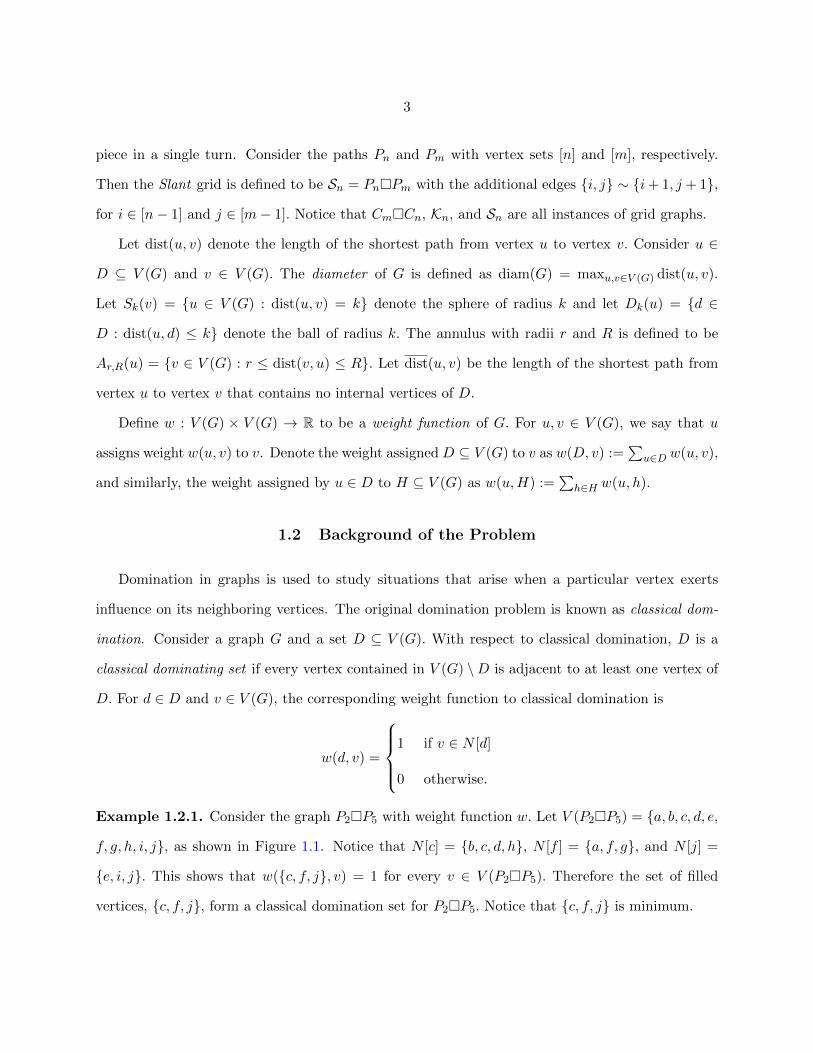
Example 1.2.1. Consider the graph P2�P5 with weight function w. Let V (P2�P5) = {a, b, c, d, e,

f, g, h, i, j}, as shown in Figure 1.1. Notice that N [c] = {b, c, d, h}, N [f ] = {a, f, g}, and N [j] =

{e, i, j}. This shows that w({c, f, j}, v) = 1 for every v ∈ V (P2�P5). Therefore the set of filled

vertices, {c, f, j}, form a classical domination set for P2�P5. Notice that {c, f, j} is minimum.

4

f g h i j

a b c d e

Figure 1.1 Filled vertices form a classical domination set for the graph P2�P5

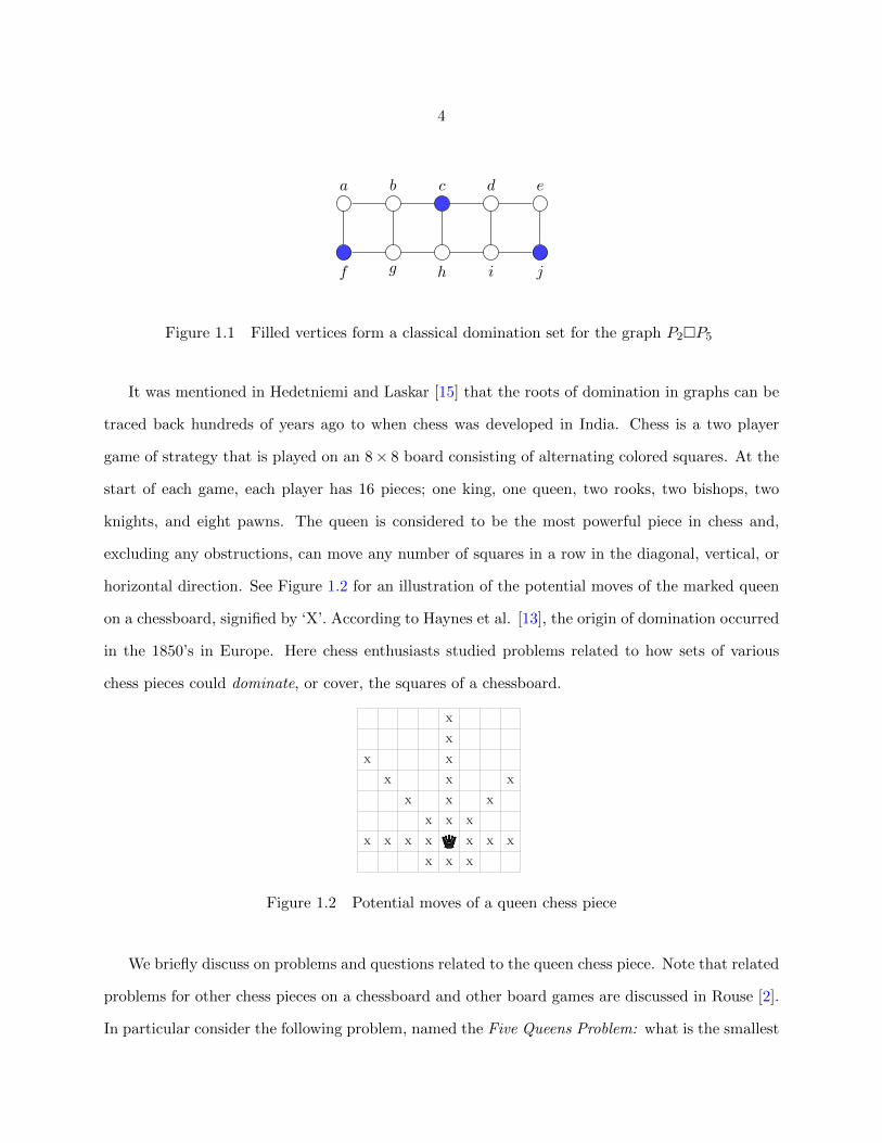
It was mentioned in Hedetniemi and Laskar [15] that the roots of domination in graphs can be

traced back hundreds of years ago to when chess was developed in India. Chess is a two player

game of strategy that is played on an 8× 8 board consisting of alternating colored squares. At the

start of each game, each player has 16 pieces; one king, one queen, two rooks, two bishops, two

knights, and eight pawns. The queen is considered to be the most powerful piece in chess and,

excluding any obstructions, can move any number of squares in a row in the diagonal, vertical, or

horizontal direction. See Figure 1.2 for an illustration of the potential moves of the marked queen

on a chessboard, signified by ‘X’. According to Haynes et al. [13], the origin of domination occurred

in the 1850’s in Europe. Here chess enthusiasts studied problems related to how sets of various

chess pieces could dominate, or cover, the squares of a chessboard.

QQQQX

X

X

X

X

X

X

X X X X X X X

X

X

X

X

X

X

X

X

X

Figure 1.2 Potential moves of a queen chess piece

We briefly discuss on problems and questions related to the queen chess piece. Note that related

problems for other chess pieces on a chessboard and other board games are discussed in Rouse [2].

In particular consider the following problem, named the Five Queens Problem: what is the smallest

5

number of queen chess pieces needed to ensure that every square on a standard chessboard can be

reached by a queen? In [2], it was mentioned that the solution to the Five Queens Problem was

five, and Figure 1.3 shows one such solution.

QQQQ

Q

Q

Q

Q

Figure 1.3 Solution to the Five Queens Problem

In the mid 1900’s the books, Theory of Graphs and its Applications [3] and Theory of Graphs

[19], were published. These two books clearly defined domination in graphs and created a solid

foundation of theory to build upon. In 1975 a survey paper on domination titled, Towards a theory

of domination in graphs [7], was published. A comprehensive bibliography [14] of over 300 citations

was created in 1988 to track all the results in the area. The authors of [7] were credited in [14] for

the desire to ‘get the ball rolling’ within the area of domination and inciting a large interest amongst

mathematicians to study domination problems. It was highlighted in [14] that the numerous real

world problems that domination modeled and the various parameters that were constructed from

domination helped to the increase the popularity of this area.

1.3 Review of Literature

1.3.1 Classical Domination

In this section, selected results from classical domination are discussed. One of the first basic

results within the area of domination came from Ore [19] in the following theorem.

Theorem 1.3.1. [19] Any graph G with δ(G) ≥ 1 has a dominating set D such that its complement

D is also a dominating set.

6

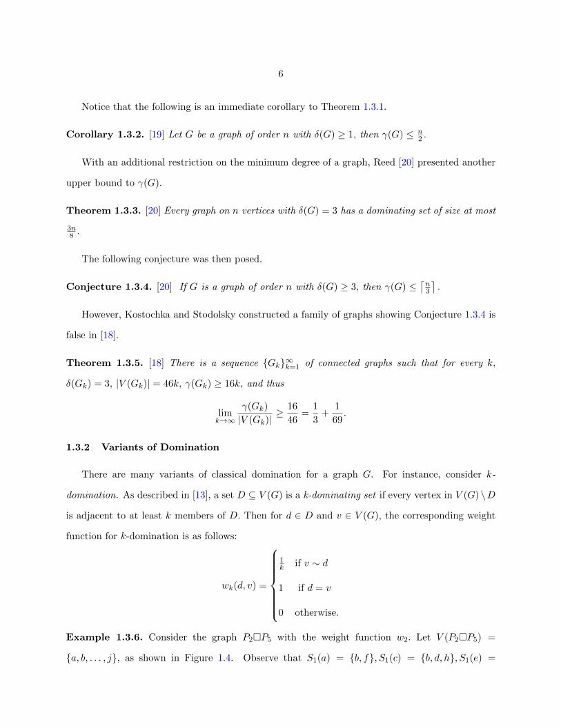
Notice that the following is an immediate corollary to Theorem 1.3.1.

Corollary 1.3.2. [19] Let G be a graph of order n with δ(G) ≥ 1, then γ(G) ≤ n2 .

With an additional restriction on the minimum degree of a graph, Reed [20] presented another

upper bound to γ(G).

Theorem 1.3.3. [20] Every graph on n vertices with δ(G) = 3 has a dominating set of size at most

3n8 .

The following conjecture was then posed.

Conjecture 1.3.4. [20] If G is a graph of order n with δ(G) ≥ 3, then γ(G) ≤⌈n3

⌉.

However, Kostochka and Stodolsky constructed a family of graphs showing Conjecture 1.3.4 is

false in [18].

Theorem 1.3.5. [18] There is a sequence {Gk}∞k=1 of connected graphs such that for every k,

δ(Gk) = 3, |V (Gk)| = 46k, γ(Gk) ≥ 16k, and thus

limk→∞

γ(Gk)

|V (Gk)|≥ 16

46=

1

3+

1

69.

1.3.2 Variants of Domination

There are many variants of classical domination for a graph G. For instance, consider k-

domination. As described in [13], a set D ⊆ V (G) is a k-dominating set if every vertex in V (G)\D

is adjacent to at least k members of D. Then for d ∈ D and v ∈ V (G), the corresponding weight

function for k-domination is as follows:

wk(d, v) =

1k if v ∼ d

1 if d = v

0 otherwise.

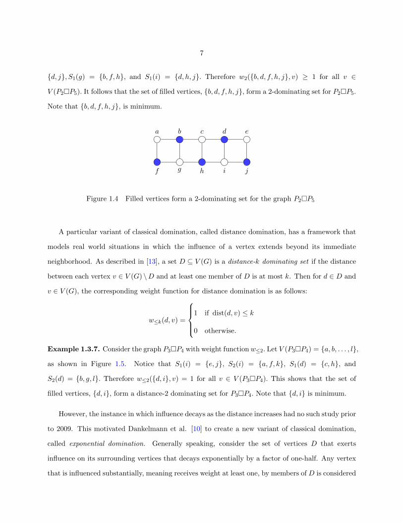
Example 1.3.6. Consider the graph P2�P5 with the weight function w2. Let V (P2�P5) =

{a, b, . . . , j}, as shown in Figure 1.4. Observe that S1(a) = {b, f}, S1(c) = {b, d, h}, S1(e) =

7

{d, j}, S1(g) = {b, f, h}, and S1(i) = {d, h, j}. Therefore w2({b, d, f, h, j}, v) ≥ 1 for all v ∈

V (P2�P5). It follows that the set of filled vertices, {b, d, f, h, j}, form a 2-dominating set for P2�P5.

Note that {b, d, f, h, j}, is minimum.

f g h i j

a b c d e

Figure 1.4 Filled vertices form a 2-dominating set for the graph P2�P5

A particular variant of classical domination, called distance domination, has a framework that

models real world situations in which the influence of a vertex extends beyond its immediate

neighborhood. As described in [13], a set D ⊆ V (G) is a distance-k dominating set if the distance

between each vertex v ∈ V (G) \D and at least one member of D is at most k. Then for d ∈ D and

v ∈ V (G), the corresponding weight function for distance domination is as follows:

w≤k(d, v) =

1 if dist(d, v) ≤ k

0 otherwise.

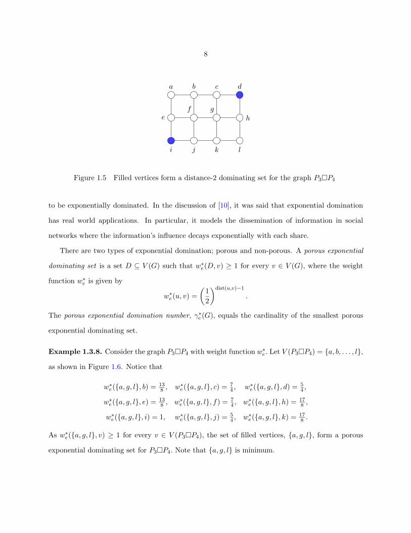
Example 1.3.7. Consider the graph P3�P4 with weight function w≤2. Let V (P3�P4) = {a, b, . . . , l},

as shown in Figure 1.5. Notice that S1(i) = {e, j}, S2(i) = {a, f, k}, S1(d) = {c, h}, and

S2(d) = {b, g, l}. Therefore w≤2({d, i}, v) = 1 for all v ∈ V (P3�P4). This shows that the set of

filled vertices, {d, i}, form a distance-2 dominating set for P3�P4. Note that {d, i} is minimum.

However, the instance in which influence decays as the distance increases had no such study prior

to 2009. This motivated Dankelmann et al. [10] to create a new variant of classical domination,

called exponential domination. Generally speaking, consider the set of vertices D that exerts

influence on its surrounding vertices that decays exponentially by a factor of one-half. Any vertex

that is influenced substantially, meaning receives weight at least one, by members of D is considered

8

i j k l

e h

a b c d

f g

Figure 1.5 Filled vertices form a distance-2 dominating set for the graph P3�P4

to be exponentially dominated. In the discussion of [10], it was said that exponential domination

has real world applications. In particular, it models the dissemination of information in social

networks where the information’s influence decays exponentially with each share.

There are two types of exponential domination; porous and non-porous. A porous exponential

dominating set is a set D ⊆ V (G) such that w∗e(D, v) ≥ 1 for every v ∈ V (G), where the weight

function w∗e is given by

w∗e(u, v) =

(1

2

)dist(u,v)−1.

The porous exponential domination number, γ∗e (G), equals the cardinality of the smallest porous

exponential dominating set.

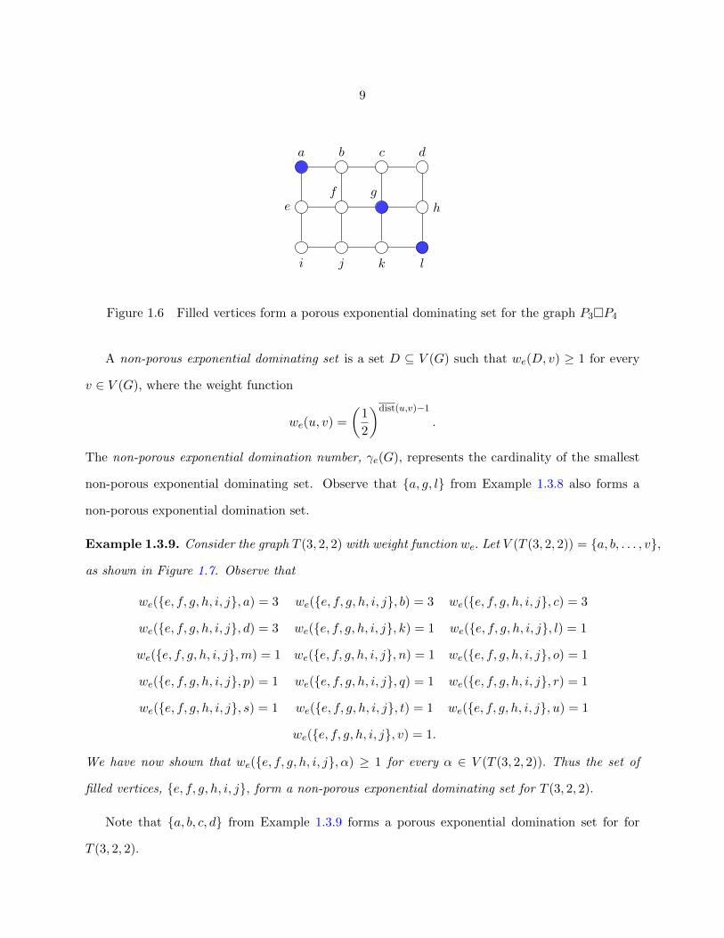
Example 1.3.8. Consider the graph P3�P4 with weight function w∗e . Let V (P3�P4) = {a, b, . . . , l},

as shown in Figure 1.6. Notice that

w∗e({a, g, l}, b) = 138 , w∗e({a, g, l}, c) = 7

4 , w∗e({a, g, l}, d) = 54 ,

w∗e({a, g, l}, e) = 138 , w∗e({a, g, l}, f) = 7

4 , w∗e({a, g, l}, h) = 178 ,

w∗e({a, g, l}, i) = 1, w∗e({a, g, l}, j) = 54 , w∗e({a, g, l}, k) = 17

8 .

As w∗e({a, g, l}, v) ≥ 1 for every v ∈ V (P3�P4), the set of filled vertices, {a, g, l}, form a porous

exponential dominating set for P3�P4. Note that {a, g, l} is minimum.

9

i j k l

e h

a b c d

f g

Figure 1.6 Filled vertices form a porous exponential dominating set for the graph P3�P4

A non-porous exponential dominating set is a set D ⊆ V (G) such that we(D, v) ≥ 1 for every

v ∈ V (G), where the weight function

we(u, v) =

(1

2

)dist(u,v)−1.

The non-porous exponential domination number, γe(G), represents the cardinality of the smallest

non-porous exponential dominating set. Observe that {a, g, l} from Example 1.3.8 also forms a

non-porous exponential domination set.

Example 1.3.9. Consider the graph T (3, 2, 2) with weight function we. Let V (T (3, 2, 2)) = {a, b, . . . , v},

as shown in Figure 1.7. Observe that

we({e, f, g, h, i, j}, a) = 3 we({e, f, g, h, i, j}, b) = 3 we({e, f, g, h, i, j}, c) = 3

we({e, f, g, h, i, j}, d) = 3 we({e, f, g, h, i, j}, k) = 1 we({e, f, g, h, i, j}, l) = 1

we({e, f, g, h, i, j},m) = 1 we({e, f, g, h, i, j}, n) = 1 we({e, f, g, h, i, j}, o) = 1

we({e, f, g, h, i, j}, p) = 1 we({e, f, g, h, i, j}, q) = 1 we({e, f, g, h, i, j}, r) = 1

we({e, f, g, h, i, j}, s) = 1 we({e, f, g, h, i, j}, t) = 1 we({e, f, g, h, i, j}, u) = 1

we({e, f, g, h, i, j}, v) = 1.

We have now shown that we({e, f, g, h, i, j}, α) ≥ 1 for every α ∈ V (T (3, 2, 2)). Thus the set of

filled vertices, {e, f, g, h, i, j}, form a non-porous exponential dominating set for T (3, 2, 2).

Note that {a, b, c, d} from Example 1.3.9 forms a porous exponential domination set for for

T (3, 2, 2).

10

k l m n o p q r s t u v

e f g h i j

b c d

a

Figure 1.7 Filled vertices form a non-porous exponential dominating set for the graph

T (3, 2, 2).

1.3.3 Exponential Domination

The other variants of classical domination rely solely on the local influence of their respective

dominating vertices to dominate neighboring vertices. Exponential domination is the only such

framework in which the influence of an exponential dominating vertex is global with respect to

other vertices. There are limited results on non-porous exponential domination and even less for

porous exponential domination. As mentioned in Henning et al. [17], the fact that exponential

domination is the only global variant of domination, and the difficulty in studying such a concept,

may be a possible explanation to the lack of results in the area.

We now discuss notable findings in exponential domination. Immediate results from the def-

inition of exponential domination noted in [10] are that for a graph G, γe(G) = 1 if and only if

γ(G) = 1 and

γ∗e (G) ≤ γe(G) ≤ γ(G). (1.3.1)

For the remainder of the dissertation, we focus only on porous and non-porous exponential

domination. For the sake of simplicity, we use the weight function w∗ to represent w∗e , the weight

function for porous exponential domination and w to represent we, the weight function for non-

11

porous exponential domination. Elementary results for Pn, the path on n vertices and Cn, the cycle

on n vertices, are stated in the following lemma and proposition.

Lemma 1.3.10. [10] For every integer n,

γ∗e (Pn) = γe(Pn) =

⌈n+ 1

4

⌉.

Proposition 1.3.11. [10] For every integer n ≥ 3,

γe(Cn) =

2 if n = 4⌈n4

⌉if n 6= 4.

The results discussed in [10] focused mainly on non-porous exponential domination. Here porous

exponential domination was used to determine a lower bound on the non-porous exponential dom-

ination number. The general upper and lower bounds for the non-porous exponential domination

number are given in the following theorem.

Theorem 1.3.12. [10] If G is a connected graph of order n and diameter diam(G), then⌈diam(G) + 2

4

⌉≤ γe(G) ≤ 2

5(n+ 2)

The proof of Theorem 1.3.12 is split into two parts, one determining the lower bound and

the other establishing the upper bound. Note that in each part, the global nature of exponential

domination is localized. The lower bound is shown via contradiction. Through the application of

several minor lemmas, it is shown that γe(G) < γ∗e (G), which contradicts (1.3.1). The proof of the

upper bound utilizes the fact that T, the spanning tree of G, has the property that γe(G) ≤ γe(T ).

Through a detailed case analysis, it is shown that the upper bound holds. There is additional

discussion on the sharpness of the bounds determined in Theorem 1.3.12. Observe that Lemma

1.3.10 shows that the lower bound is sharp. Through brute force, it was verified that there is no

tree T of order n ≤ 10 with the property that γe(T ) = 2(n+2)5 . However, brute force could not be

applied for trees of order n > 10. Through the use of computers, [10] searched to find trees so that

the value γe(T )n+2 is maximized. The best result for the upper bound of the non-porous exponential

12

domination number of trees occurred via the construction of an infinite family of trees T such

that limn→∞γe(T )n+2 = 144

379 ≈ 0.380, for T ∈ T , with n denoting the order of T. Outside of infinite

families, it was shown that the tree T0 = T (2, 3, 3, 4, 3, 4, 2, 1) of order n = 375 has γe(T0) = 144,

so γe(T0)n+2 = 144

377 ≈ 0.382. Therefore the upper bound for Theorem 1.3.12 is not known to be sharp.

In the concluding remarks, [10] posed the following two open questions:

1. Let T be a tree. Is there a polynomial-time algorithm to determine γe(T ).

2. Under what conditions is γe(G) = γ(G)?

The papers Bessy et al. [4], Henning et al. [16] and [17] address the open questions posed in [10].

We now summarize the main results from these papers. First, non-porous exponential domination

in subcubic graphs was studied [4]. Here the authors were able to manipulate properties of subcubic

graphs that somewhat localized exponential domination. This resulted in an upper bound for the

weight that a vertex receives from the exponential dominating set, which simplified determining

the non-porous exponential domination number of subcubic graphs. The following theorem is the

best result for the lower and upper bounds of the non-porous exponential domination number of

any subcubic graph G, and it is shown that the upper bound is tight.

Theorem 1.3.13. [4] If G is a connected subcubic graph of order n, then

n

6 log2(n+ 2) + 4≤ γe(G) ≤ n+ 2

3.

Similarly as for the upper bound in Theorem 1.3.12, [4] used that the spanning tree H of G

has the property that γe(G) ≤ γe(H). The upper bound was shown for all trees through the use

of induction on the order the tree T. Putting it all together gave that the upper bound held for

all graphs. The lower bound in Theorem 1.3.13 was shown to be true through the use of a clever

counting argument that manipulated the weight a particular vertex received from the non-porous

exponential dominating set, along with the use of an auxiliary theorem.

In the remainder of [4], there is a focus on the complexity of the non-porous exponential domi-

nation number of subcubic trees.

13

Theorem 1.3.14. [4] Given a subcubic tree T, γe(T ) can be determined in polynomial time.

Notice that Theorem 1.3.14 shows that there exists a polynomial time algorithm that computes

the non-porous exponential domination number of a subcubic tree, and answers the first open

question posed in [10] for subcubic trees. Further, [4] establishes that determining a minimum

non-porous exponential dominating set of a given subcubic graph is APX-hard. However no such

algorithm is known for general trees, nor for the porous exponential domination number of subcubic

trees.

In [16], the second open problem from [10] is addressed. The hereditary class G is the set of

graphs G for which γe(H) = γ(H) for every induced subgraph H of G [16]. Through the use

of minimal forbidden induced subgraphs, the authors characterize a large subclass of G. Theorem

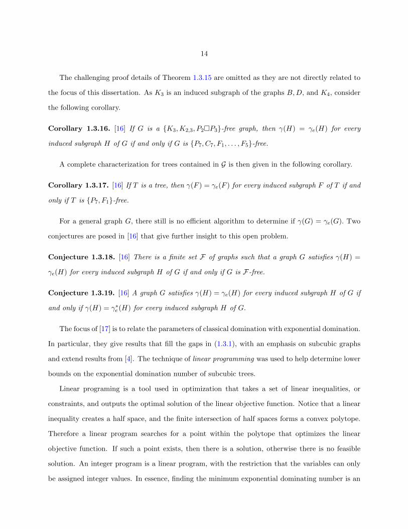
1.3.15, Corollary 1.3.16, and Corollary 1.3.17 use the graphs depicted in Figure 1.8.

Figure 1.8 The graphs K3, K2,3, P2�P3, B, D, K4, and F1, . . . , F5 from [16]

Theorem 1.3.15. [16] If G is a {B,D,K4,K2,3, P2�P3}-free graph, then γ(H) = γe(H) for every

induced subgraph H of G if and only if G is {P7, C7, F1, . . . , F5}-free.

14

The challenging proof details of Theorem 1.3.15 are omitted as they are not directly related to

the focus of this dissertation. As K3 is an induced subgraph of the graphs B,D, and K4, consider

the following corollary.

Corollary 1.3.16. [16] If G is a {K3,K2,3, P2�P3}-free graph, then γ(H) = γe(H) for every

induced subgraph H of G if and only if G is {P7, C7, F1, . . . , F5}-free.

A complete characterization for trees contained in G is then given in the following corollary.

Corollary 1.3.17. [16] If T is a tree, then γ(F ) = γe(F ) for every induced subgraph F of T if and

only if T is {P7, F1}-free.

For a general graph G, there still is no efficient algorithm to determine if γ(G) = γe(G). Two

conjectures are posed in [16] that give further insight to this open problem.

Conjecture 1.3.18. [16] There is a finite set F of graphs such that a graph G satisfies γ(H) =

γe(H) for every induced subgraph H of G if and only if G is F-free.

Conjecture 1.3.19. [16] A graph G satisfies γ(H) = γe(H) for every induced subgraph H of G if

and only if γ(H) = γ∗e (H) for every induced subgraph H of G.

The focus of [17] is to relate the parameters of classical domination with exponential domination.

In particular, they give results that fill the gaps in (1.3.1), with an emphasis on subcubic graphs

and extend results from [4]. The technique of linear programming was used to help determine lower

bounds on the exponential domination number of subcubic trees.

Linear programing is a tool used in optimization that takes a set of linear inequalities, or

constraints, and outputs the optimal solution of the linear objective function. Notice that a linear

inequality creates a half space, and the finite intersection of half spaces forms a convex polytope.

Therefore a linear program searches for a point within the polytope that optimizes the linear

objective function. If such a point exists, then there is a solution, otherwise there is no feasible

solution. An integer program is a linear program, with the restriction that the variables can only

be assigned integer values. In essence, finding the minimum exponential dominating number is an

15

optimization problem because the aim is to find the fewest exponential dominating vertices that

exponentially dominate the remaining vertices.

The following integer program is formulated for a graph so that the optimum value is γ∗e (G).

Integer Program 1.3.20. [17]

min∑

u∈V (G)

x(u)

s.t.∑

u∈V (G)

(1

2

)dist(u,v)−1x(u) ≥ 1 ∀v ∈ V (G)

x(u) ∈ {0, 1} ∀u ∈ V (G).

A new exponential domination parameter called the fractional porous exponential domination

number, denoted γ∗e,f (G), is introduced in [17]. The following linear program is a relaxation of

Integer Program 1.3.20, and the corresponding optimum value is equivalent to γ∗e,f (G).

Linear Program 1.3.21. [17]

min∑

u∈V (G)

x(u)

s.t.∑

u∈V (G)

(1

2

)dist(u,v)−1x(u) ≥ 1 ∀v ∈ V (G)

x(u) ≥ 0 ∀u ∈ V (G).

A notable result using the concept of the fractional porous exponential domination number of

a graph is summarized in the following theorem.

Theorem 1.3.22. [17] If T is a subcubic tree of order n, then γ∗e,f (T ) = n+26 .

The value of γ∗e,f (T ) determined in Theorem 1.3.22 is a consequence of applying Linear Program

1.3.21 to subcubic trees. The corresponding objective function is∑

u∈V (T )

x(u), where

x(u) =

13 , if u is an endvertex of T

16 , if u has degree 2 in T

0, if u has degree 3 in T.

16

The bounds of the non-porous exponential domination number of a connected graph from

Theorem 1.3.12 were improved in Bessy et al. [5]. In particular, the upper bound was strengthened

with the following theorem.

Theorem 1.3.23. [5] If G is a connected graph of order n, then γe(G) ≤ 43108(n+ 2).

The proof of Theorem 1.3.23 is similar to the proof of Theorem 1.3.12. Since 43108 is approximately

25 , we see that [5] did not drastically improve the bound. To sharpen the bound any further, a

complex case analysis would be needed. It was also acknowledged in [5] that the process of localizing

the global influence of exponential dominating vertices does not necessarily produce the best upper

bound.

Although most results related to exponential domination have had a focus on subcubic graphs,

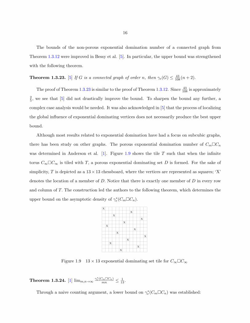
there has been study on other graphs. The porous exponential domination number of Cm�Cn

was determined in Anderson et al. [1]. Figure 1.9 shows the tile T such that when the infinite

torus C∞�C∞ is tiled with T, a porous exponential dominating set D is formed. For the sake of

simplicity, T is depicted as a 13× 13 chessboard, where the vertices are represented as squares; ‘X’

denotes the location of a member of D. Notice that there is exactly one member of D in every row

and column of T. The construction led the authors to the following theorem, which determines the

upper bound on the asymptotic density of γ∗e (Cm�Cn).

X

X

X

X

X

X

X

X

X

X

X

X

X

Figure 1.9 13× 13 exponential dominating set tile for C∞�C∞

Theorem 1.3.24. [1] limm,n→∞γ∗e (Cm�Cn)

mn ≤ 113 .

Through a naive counting argument, a lower bound on γ∗e (Cm�Cn) was established:

17

Theorem 1.3.25. [1] For all m,n > 3,

mn

15.875< γ∗e (Cm�Cn).

The results of Theorems 1.3.24 and 1.3.25 lead [1] to Conjecture 1.3.26. Observe that if this

conjecture is proven to be true, then the exact value of γ∗e (Cm�Cn) will be known.

Conjecture 1.3.26. For all m and n, γe(Cm�Cn)mn ≥ 1

13 and this bound is sharp (take m = n = 13).

In the unpublished work of Bozeman et al. [6], the lower bound for γ∗e (Cm�Cn) determined in

Theorem 1.3.25 was improved through the use of linear programming. Notice that Theorem 1.3.27

further supports Conjecture 1.3.26.

Theorem 1.3.27. [6] For all m,n ≥ 11,

mn

13.761891939197298≤ γ∗e (Cm�Cn).

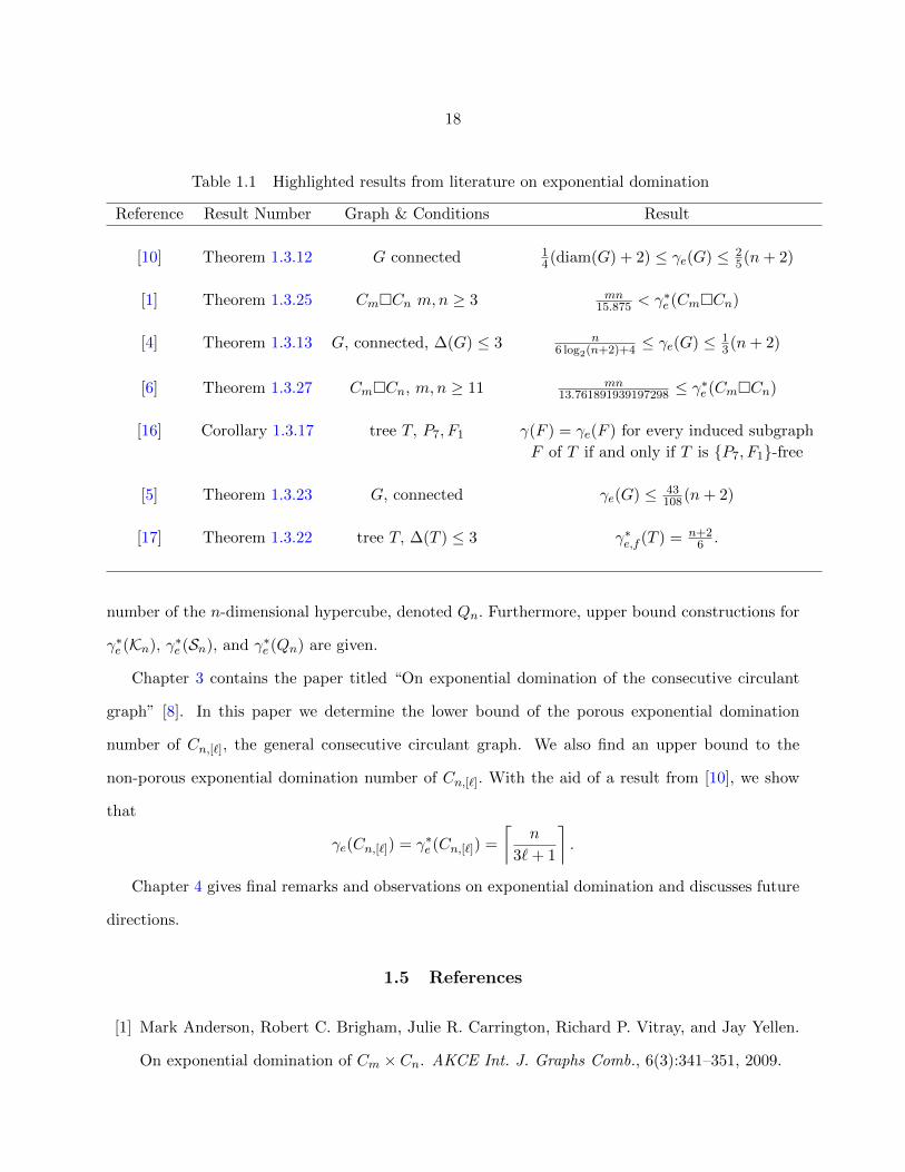
In conclusion, there are a number of results already known within the area of exponential domi-

nation. Table 1.1 contains a summary of the main results from articles on exponential domination.

The entries in the table are given in ascending order with respect to the year published or posted

online.

1.4 Organization of the Dissertation

This dissertation is written under the format of a collection of papers submitted to journals.

Chapter 1 presents definitions, discusses the history of exponential domination, and summarizes

the literature within this area.

Chapter 2 contains the paper “A linear programming method for exponential domination” [9]. In

this paper we first describe a technique to find a lower bound for the porous exponential domination

number of any graph. A linear programming method is given to determine the lower bound of the

porous exponential domination number of the King grid, denoted Kn, and the Slant grid, denoted

Sn. Another method is applied to construct a lower bound to the porous exponential domination

18

Table 1.1 Highlighted results from literature on exponential domination

Reference Result Number Graph & Conditions Result

[10] Theorem 1.3.12 G connected 14(diam(G) + 2) ≤ γe(G) ≤ 2

5(n+ 2)

[1] Theorem 1.3.25 Cm�Cn m,n ≥ 3 mn15.875 < γ∗e (Cm�Cn)

[4] Theorem 1.3.13 G, connected, ∆(G) ≤ 3 n6 log2(n+2)+4 ≤ γe(G) ≤ 1

3(n+ 2)

[6] Theorem 1.3.27 Cm�Cn, m, n ≥ 11 mn13.761891939197298 ≤ γ

∗e (Cm�Cn)

[16] Corollary 1.3.17 tree T, P7, F1 γ(F ) = γe(F ) for every induced subgraph

F of T if and only if T is {P7, F1}-free

[5] Theorem 1.3.23 G, connected γe(G) ≤ 43108(n+ 2)

[17] Theorem 1.3.22 tree T, ∆(T ) ≤ 3 γ∗e,f (T ) = n+26 .

number of the n-dimensional hypercube, denoted Qn. Furthermore, upper bound constructions for

γ∗e (Kn), γ∗e (Sn), and γ∗e (Qn) are given.

Chapter 3 contains the paper titled “On exponential domination of the consecutive circulant

graph” [8]. In this paper we determine the lower bound of the porous exponential domination

number of Cn,[`], the general consecutive circulant graph. We also find an upper bound to the

non-porous exponential domination number of Cn,[`]. With the aid of a result from [10], we show

that

γe(Cn,[`]) = γ∗e (Cn,[`]) =

⌈n

3`+ 1

⌉.

Chapter 4 gives final remarks and observations on exponential domination and discusses future

directions.

1.5 References

[1] Mark Anderson, Robert C. Brigham, Julie R. Carrington, Richard P. Vitray, and Jay Yellen.

On exponential domination of Cm × Cn. AKCE Int. J. Graphs Comb., 6(3):341–351, 2009.

19

[2] Walter William Rouse Ball. Mathematical recreations and essays. London : Macmillan, 7

edition, 1917.

[3] Claude Berge. Theory of Graphs and its Applications. Methuen, London, 1962.

[4] Stephane Bessy, Pascal Ochem, and Dieter Rautenbach. Exponential domination in subcubic

graphs. Electr. J. Comb., 23:P4.42, 2016.

[5] Stephane Bessy, Pascal Ochem, and Dieter Rautenbach. Bounds on the exponential domination

number. Discrete Math., 340(3):494–503, 2017.

[6] Chassidy Bozeman, Joshua Carlson, Michael Dairyko, Derek Young, and Michael Young. Lower

bounds for the exponential domination number of Cm × Cn. arXiv:1803.01933, 2018.

[7] Ernest J. Cockayne and Stephen T. Hedetniemi. Towards a theory of domination in graphs.

Networks, 7:247–261, 1977.

[8] Michael Dairyko and Michael Young. On exponential domination of the consecuative circulant

graph. arXiv:1712.05429, 2017.

[9] Michael Dairyko and Michael Young. A Linear programming method for exponential domina-

tion. arXiv:1801.06404, 2018.

[10] Peter Dankelmann, David Day, David Erwin, Simon Mukwembi, and Henda Swart. Domina-

tion with exponential decay. Discrete Math., 309(19):5877–5883, 2009.

[11] Reinhard Diestel. Graph Theory, 4th Edition, volume 173 of Graduate texts in mathematics.

Springer, 2012.

[12] Teresa W. Haynes, Stephen T. Hedetniemi, and Peter J. Slater. Domination in graphs :

advanced topics. New York : Marcel Dekker, 1997.

[13] Teresa W. Haynes, Stephen T. Hedetniemi, and Peter J. Slater. Fundamentals of domination

in graphs, volume 208 of Monographs and Textbooks in Pure and Applied Mathematics. Marcel

Dekker, Inc., New York, 1998.

20

[14] Stephen T. Hedetniemi and Renu C. Laskar. Bibliography on domination in graphs and some

basic definitions of domination parameters. Discrete Mathematics, 86(1):257 – 277, 1990.

[15] Stephen T. Hedetniemi and Renu C. Laskar. Topics on domination. Annals of discrete math-

ematics. Elsevier, Burlington, MA, 1991.

[16] Michael A. Henning, Simon Jager, and Dieter Rautenbach. Hereditary Equality of Domination

and Exponential Domination. Discussiones Mathematicae Graph Theory, 2016.

[17] Michael A. Henning, Simon Jager, and Dieter Rautenbach. Relating domination, exponential

domination, and porous exponential domination. Discrete Optim., 23:81–92, 2017.

[18] Alexandr V. Kostochka and Burak Y. Stodolsky. On domination in connected cubic graphs.

Discrete Mathematics, 304(1):45 – 50, 2005.

[19] Oystein Ore. Theory of graphs. Colloquium publications (American Mathematical Society)

v. 38. American Mathematical Society, Providence, R.I., 3d printing with corrections. edition,

1967.

[20] Bruce Reed. Paths, stars, and the number three. Combinatorics, Probability, and Computing,

5:277 – 295, September 1995.

21

CHAPTER 2. A LINEAR PROGRAMMING METHOD FOR

EXPONENTIAL DOMINATION

Modified form of a submitted paper

Michael Dairyko1 and Michael Young

Abstract

For a graphG, the setD ⊆ V (G) is a porous exponential dominating set if 1 ≤∑

d∈D (2)1−dist(d,v)

for every v ∈ V (G), where dist(d, v) denotes the length of the shortest dv path. The porous expo-

nential dominating number of G, denoted γ∗e (G), is the minimum cardinality of a porous exponential

dominating set. For any graph G, a technique is derived to determine a lower bound for γ∗e (G).

Specifically for a grid graph H, linear programing is used to sharpen bound found through the lower

bound technique. Lower and upper bounds are determined for the porous exponential domination

number of the King Grid Kn, the Slant Grid Sn, and the n-dimensional hypercube Qn.

AMS 2010 Subject Classification: Primary 05C69; Secondary 90C05

Keywords: porous exponential domination, linear programming, grid graphs, n-dimensional

hypercube

2.1 Introduction

Domination in graphs is a tool used to model situations in which a vertex exerts influence on its

neighboring vertices. For a graph G, a set D ⊆ V (G) is a dominating set if every vertex contained

in V (G) \D is adjacent to at least one vertex of D. The domination number, denoted γ(G), is the

cardinality of a minimum domination set.

1Primary Researcher and Author.

22

Exponential domination was first introduced in [6] and is a variant of domination that models

situations in which the influence an object exerts decreases exponentially as the distance increases.

In particular exponential domination models the dissemination of information in social networks

where the information’s influence decays exponentially with each share [6]. Therefore, exponential

domination analyzes objects with a global influence. Other variants of domination investigate

objects with local influence. There are two parameters within exponential domination; porous

and non-porous. This paper focuses on porous exponential domination. A porous exponential

dominating set is a set D ⊆ V (G) such that w∗(D, v) ≥ 1 for every v ∈ V (G), where the weight

function w∗ is given by w∗(u, v) = 21−dist(u,v) and dist(u, v) represents the length of the shortest

uv path. The porous exponential domination number of G, denoted by γ∗e (G), is the cardinality of

a minimum porous exponential dominating set. For the sake of simplicity, we will refer to porous

exponential domination as exponential domination. See Section 2.1.1 for technical definitions.

Section 2.2 develops a technique to determine the lower bound of the exponential domination

number of any graph. Furthermore, with respect to grid graphs, a method using linear programing

sharpens the lower bound. Section 2.3 applies the lower bound technique described in Section 2.2,

to find lower bounds for the exponential domination number of the King grid Kn, the Slant grid

Sn, and the n-dimensional hypercube Qn. Upper bound constructions are then found for γ∗e (Kn),

γ∗e (Sn) and γ∗e (Qn).

2.1.1 Preliminaries

All graphs are simple and undirected. A graph G = (V (G), E(G)) is an ordered pair that

is formed by a set of vertices V (G) and a set of edges E(G), where an edge is the two element

subset of vertices. For the two sets A and B, the Cartesian product of A and B is defined to

be A × B = {(a, b) : a ∈ A and b ∈ B}. Consider the graph G and the set D ⊆ V (G). Let

w : V (G)× V (G)→ R be a weight function. For u, v ∈ V (G), we say that u assigns weight w(u, v)

to v. Denote the weight assigned by D to v as w(D, v) :=∑

d∈D w(d, v), and similarly, the weight

assigned by d ∈ D to H ⊆ V (G) as w(d,H) :=∑

h∈H w(d, h). Let m(G) = maxd∈D w(d, V (G)).

23

The pair (D,w) dominates G if w(D, v) ≥ 1 for all v ∈ V (G). The excess weight that the vertex v

receives from D is defined as exc(D, v) = w(D, v) − 1. We denote exc(D) =∑

v∈V (G) exc(D, v) to

be the total excess weight that D sends out. Let Sk(v) = {u ∈ V (G) : dist(u, v) = k} denote the

sphere of radius k.

Linear programing is an optimization technique that takes a set of linear inequalities, or con-

straints, and finds the best solution of a linear objective function. An integer program is a linear

program, with the restriction the variables can only be assigned integer values. Observe that γ∗e (G)

is equivalent to finding the optimal value of the following integer program introduced by Henning

et al.:

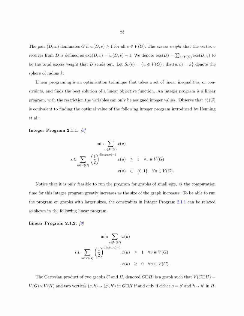
Integer Program 2.1.1. [9]

min∑

u∈V (G)

x(u)

s.t.∑

u∈V (G)

(1

2

)dist(u,v)−1x(u) ≥ 1 ∀v ∈ V (G)

x(u) ∈ {0, 1} ∀u ∈ V (G).

Notice that it is only feasible to run the program for graphs of small size, as the computation

time for this integer program greatly increases as the size of the graph increases. To be able to run

the program on graphs with larger sizes, the constraints in Integer Program 2.1.1 can be relaxed

as shown in the following linear program.

Linear Program 2.1.2. [9]

min∑

u∈V (G)

x(u)

s.t.∑

u∈V (G)

(1

2

)dist(u,v)−1x(u) ≥ 1 ∀v ∈ V (G)

x(u) ≥ 0 ∀u ∈ V (G).

The Cartesian product of two graphs G and H, denoted G�H, is a graph such that V (G�H) =

V (G)×V (H) and two vertices (g, h) ∼ (g′, h′) in G�H if and only if either g = g′ and h ∼ h′ in H,

24

or h = h′ and g ∼ g′ in G. Let Gm,n = Pm�Pn be the standard grid. A grid graph is the standard

grid with possibly additional edges added in a regular pattern. Notice that linear programming is

a natural technique to apply to grid graphs. Observe that asymptotically, Gm,n is equivalent to the

torus Cm�Cn, which yields the same lower bound for the corresponding exponential domination

number.

Figure 2.1 An illustration of K5, Q4, and S5

The strong product of two graphs G and H is the graph G�H for which V (G�H) = V (G)×

V (H) and two distinct vertices are adjacent whenever in both coordinate places the vertices are

adjacent or equal in the corresponding graph. The King grid is defined as Kn = Pn � Pn. Let

[n] = {1, 2, . . . , n}. Consider the paths Pn and Pm with vertex sets [n] and [m], respectively. Then

the Slant grid is defined to be Sn = Pn�Pm with the additional edges {i, j} ∼ {i + 1, j + 1},

for i ∈ [n − 1] and j ∈ [m − 1]. Notice that Kn and Sn are both instances of grid graphs. The

n-dimensional hypercube graph, denoted Qn, is constructed by creating a vertex for each n-digit

binary word. Edges are formed if two vertices differ by one digit in their binary representation. See

Figure 2.1 for an illustration of K5, Q4, and S5.

2.1.2 Motivation

For m ≤ n consider Cm�Cn, the torus graph. Exponential domination of Cm�Cn was first

studied in [1]. Figure 2.2 is a visual representation of C13�C13, where X denotes a member of D,

an exponential domination set. Observe that there is one member of D in every row and column,

25

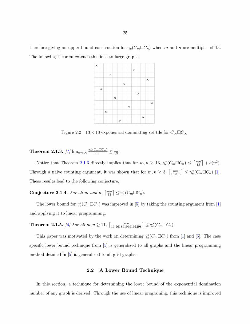
therefore giving an upper bound construction for γe(Cm�Cn) when m and n are multiples of 13.

The following theorem extends this idea to large graphs.

X

X

X

X

X

X

X

X

X

X

X

X

X

Figure 2.2 13× 13 exponential dominating set tile for C∞�C∞

Theorem 2.1.3. [1] limn→∞γ∗e (Cm�Cn)

mn ≤ 113 .

Notice that Theorem 2.1.3 directly implies that for m,n ≥ 13, γ∗e (Cm�Cn) ≤⌈mn13

⌉+ o(n2).

Through a naive counting argument, it was shown that for m,n ≥ 3,⌈

mn15.875

⌉≤ γ∗e (Cm�Cn) [1].

These results lead to the following conjecture.

Conjecture 2.1.4. For all m and n,⌈mn13

⌉≤ γ∗e (Cm�Cn).

The lower bound for γ∗e (Cm�Cn) was improved in [5] by taking the counting argument from [1]

and applying it to linear programming.

Theorem 2.1.5. [5] For all m,n ≥ 11,⌈

mn13.761891939197298

⌉≤ γ∗e (Cm�Cn).

This paper was motivated by the work on determining γ∗e (Cm�Cn) from [1] and [5]. The case

specific lower bound technique from [5] is generalized to all graphs and the linear programming

method detailed in [5] is generalized to all grid graphs.

2.2 A Lower Bound Technique

In this section, a technique for determining the lower bound of the exponential domination

number of any graph is derived. Through the use of linear programing, this technique is improved

26

specifically for grid graphs. Note that the bound in Lemma 2.2.1 is sharp if w∗(v, V (G)) = m(G)

for every v ∈ V (G).

Lemma 2.2.1. Let D be an exponential dominating set for the graph G. If k|D| ≤ exc(D), then⌈|V (G)|

m(G)− k

⌉≤ |D|.

Proof. Observe that

|V (G)| ≤∑

v∈V (G)

w(D, v) =∑d∈D

∑v∈V (G)

w(d, v) ≤ |D|m(G)− exc(G)

≤ |D|(

m(G)− exc(D)

|D|

)≤ |D| (m(G)− k) .

Remark 2.2.2. In Lemma 2.2.1, the value k is needed to compute the lower bound. For grid

graphs, linear programming can be used to determine such a value of k. Mixed Integer Linear

Program 2.2.3 is derived through the use of Linear Program 2.1.2 with two additional constraints.

See Section 2.2.1 for the construction details. Let xmin be the optimal solution found from Mixed

Integer Linear Program 2.2.3. As w∗(D, v) ≥ 1 for all v ∈ V (G), it follows that |I| < xmin.

Therefore k = xmin − |I|.

Mixed Integer Linear Program 2.2.3.

min∑i∈I

[Ax]i

s.t. Ax ≥ 1

Ax ≤ b

x ≥ 0

xi ≤ 2, i ∈ I

x1 = 2.

Remark 2.2.4. Observe that Remark 2.2.2 localizes the global nature of exponential domination.

Recall that exponential domination has a growth factor of 12 . Therefore this method can be applied

27

to the variant of exponential domination with the growth factor of 1p for p ≥ 3. Furthermore, the

method can be applied to other variants of domination to obtain a lower bound for the corresponding

domination number. However, it is unclear whether the lower bound derived will be significant.

2.2.1 Mixed Integer Linear Program Setup

The setup for Mixed Integer Linear Program 2.2.3 is now discussed. Consider the m × n grid

graph G and let D be a corresponding exponential dominating set. For a fixed d0 ∈ D and given an

odd positive integer r ≤ min{m,n}, define H to be the r× r subgrid of G centered at d0. Label the

set of vertices V (H) as {v1, v2, . . . , vr2} and let the indices of the interior vertices of H be defined

as

I ={i : vi ∈ V (H) and dist(d0, vi) <

⌊r2

⌋}.

Then for 1 ≤ k ≤ r2, define Sk = vk ∪ {u ∈ V (G \ H) : dist(u, vk) ≤ dist(u, h) ∀h ∈ V (H)} and

xk = w∗(Sk ∩D, vk). Notice that Si = vi for every i ∈ I. Therefore for 1 ≤ k, j ≤ r2, it follows that

w∗(Sk ∩D, vj) ≤ xk(12

)dist(vk,vj) . Thus, by the construction of Sk,

w∗(D, vj) ≤r2∑k=1

w∗(Sk ∩D, vj) ≤r2∑k=1

xk

(1

2

)dist(vk,vj)

.

Let A be the r2× r2 matrix such that [A]kj =(12

)dist(vk,vj) . Furthermore, let ~x = [x1, x2, . . . , xr2 ]ᵀ,

where x1 corresponds to d0, and ~w = [w∗(D, v1), w∗(D, v2), . . . , w

∗(D, vr2)]ᵀ. Then observe that

~w ≤ A~x. The aim is to minimize w∗(d0, vi) for all i ∈ I, while still satisfying that w∗(D, vi) ≥ 1.

Therefore the objective function is to minimize∑

i∈I [Ax]i, where x is a vector of r2 nonnegative

variables.

Let 0 and 1 denote the 0s and 1s vectors of length r. Then the two constraints of Linear Program

2.1.2 with respect to the grid graph construction are that Ax ≥ 1 and x ≥ 0. The remaining two

constraints of Mixed Integer Linear Program are now discussed. By construction, any member of

D assigns itself weight 2, and the remaining vertices do not have any initial weight. This gives

the first integer constraint that x1 = 2 and xi ≤ 2, for i ∈ I. Observe that it is necessary to

determine an upper bound for w∗(D, vi) for each vi ∈ V (H) so that w∗(d0, vi) can be decreased by

28

the appropriate amount. To ensure this, we want

0 ≤ w∗(d0, vi)− exc(D, vi) = w∗(d0, vi)− (w∗(D, vi)− 1).

This implies that w∗(D, vi) ≤ 1 + w∗(d0, vi). Let b be the real valued vector such that bi = 1 +(12

)dist(d0,vi)−1 for 1 ≤ i ≤ r2. Therefore, the second constraint is Ax ≤ b.

2.3 Main Results

In this section the lower bound technique discussed in Section 2.2 is applied and upper bound

constructions are found to bound the exponential domination number of the the King grid Kn,

Slant grid Sn, and n-dimensional hypercube Qn.

2.3.1 The King Grid Kn

For small values of n, the exact value of γ∗e (Kn) can be determined using Integer Program 2.1.1.

Figure 2.3 visualizes the location of the corresponding exponential dominating vertices for γ∗e (Kn),

denoted by ‘X’. See Code 2.6.1 for the corresponding SAGE code.

X

n = 2

X

n = 3

X X

n = 4

X X X

n = 5

X

X

X

X

n = 6

X

X

X

X

n = 7

X X

X

X

X X

n = 8

X X

X

X

X

X X

n = 9

X

X X

X

X

X

X

X

n = 10

Figure 2.3 Minimum exponential dominating sets of Kn, 2 ≤ n ≤ 10

29

Let D be an exponential dominating set for Kn. Notice that for d ∈ D, it follows that |Sk(v)| =

8k for k ≥ 1. Then,

w∗(d, V (Kn)) < 2 +∞∑k=1

8k

(1

2

)k−1= 2 +

(8(

1− 12

)2)

= 34.

This shows that m(Kn) < 34. This fact, along with the optimal values of k determined by Mixed

Integer Linear Program 2.2.3 can be applied with Lemma 2.2.1 to determine a lower bound for

γ∗e (Kn). See Table 2.1 for a summary of these results. Observe that for n ≥ 11, there is no feasible

solution with Mixed Integer Linear Program 2.2.3. This is caused by the constraint Ax ≤ b, since it

puts a bound on the reduction of how much weight the center vertex can send out to the remaining

interior vertices. Thus the best use of Mixed Integer Linear Program 2.2.3 will occur at n = 7.

Table 2.1 Lower Bounds for γ∗e (Kn) for small values of n

n 3 5 7 9 11

k 1 5.7806 10.6905 10.4103 ∅

γ∗e (Kn) ≥ n2

33n2

28.2194n2

23.3095n2

23.5897 ∅

Theorem 2.3.1. For all n ≥ 7,⌈

n2

23.3095033018

⌉≤ γ∗e (Kn).

Proof. Let D be a minimum exponential dominating set for Kn. For each d ∈ D, let H be the

7 × 7 grid centered at d. The corresponding solution to Mixed Integer Linear Program 2.2.3 gives

xmin = 35.6904966982. Therefore let k = 35.6904966982 − 25 = 10.6904966982 and recall that

m(Kn) < 34. Therefore result follows from Lemma 2.2.1.

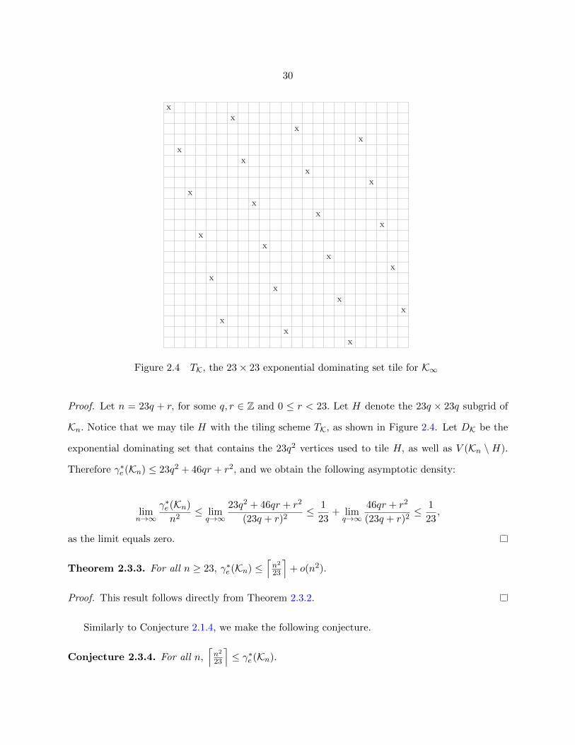
Figure 2.4 shows a construction of a 23 × 23 tile TK, where ‘X’ denotes the location of an

exponential dominating vertex. In particular, when K∞ is tiled with TK, the exponential dominating

set DK is formed. The following theorem uses TK to determines an upper bound for the asymptotic

density of γ∗e (Kn).

Theorem 2.3.2. limn→∞γ∗e (Kn)

n2≤ 1

23

30

X

X

X

X

X

X

X

X

X

X

X

X

X

X

X

X

X

X

X

X

X

X

X

Figure 2.4 TK, the 23× 23 exponential dominating set tile for K∞

Proof. Let n = 23q + r, for some q, r ∈ Z and 0 ≤ r < 23. Let H denote the 23q × 23q subgrid of

Kn. Notice that we may tile H with the tiling scheme TK, as shown in Figure 2.4. Let DK be the

exponential dominating set that contains the 23q2 vertices used to tile H, as well as V (Kn \ H).

Therefore γ∗e (Kn) ≤ 23q2 + 46qr + r2, and we obtain the following asymptotic density:

limn→∞

γ∗e (Kn)

n2≤ lim

q→∞

23q2 + 46qr + r2

(23q + r)2≤ 1

23+ limq→∞

46qr + r2

(23q + r)2≤ 1

23,

as the limit equals zero.

Theorem 2.3.3. For all n ≥ 23, γ∗e (Kn) ≤⌈n2

23

⌉+ o(n2).

Proof. This result follows directly from Theorem 2.3.2.

Similarly to Conjecture 2.1.4, we make the following conjecture.

Conjecture 2.3.4. For all n,⌈n2

23

⌉≤ γ∗e (Kn).

31

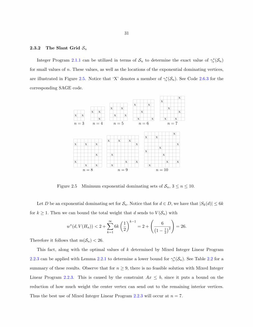
2.3.2 The Slant Grid Sn

Integer Program 2.1.1 can be utilized in terms of Sn to determine the exact value of γ∗e (Sn)

for small values of n. These values, as well as the locations of the exponential dominating vertices,

are illustrated in Figure 2.5. Notice that ‘X’ denotes a member of γ∗e (Sn). See Code 2.6.3 for the

corresponding SAGE code.

X X

n = 3

X X

X

n = 4

X X

X X

n = 5

X X

X

X X

n = 6

X

X

X

X

X X

n = 7

X X X

X

X

X X

n = 8

X X X

X

X

X X

X

n = 9

X

X X

X

X

X

X

X X

X

n = 10

Figure 2.5 Minimum exponential dominating sets of Sn, 3 ≤ n ≤ 10.

Let D be an exponential dominating set for Sn. Notice that for d ∈ D, we have that |Sk(d)| ≤ 6k

for k ≥ 1. Then we can bound the total weight that d sends to V (Sn) with

w∗(d, V (Hn)) < 2 +∞∑k=1

6k

(1

2

)k−1= 2 +

(6(

1− 12

)2)

= 26.

Therefore it follows that m(Sn) < 26.

This fact, along with the optimal values of k determined by Mixed Integer Linear Program

2.2.3 can be applied with Lemma 2.2.1 to determine a lower bound for γ∗e (Sn). See Table 2.2 for a

summary of these results. Observe that for n ≥ 9, there is no feasible solution with Mixed Integer

Linear Program 2.2.3. This is caused by the constraint Ax ≤ b, since it puts a bound on the

reduction of how much weight the center vertex can send out to the remaining interior vertices.

Thus the best use of Mixed Integer Linear Program 2.2.3 will occur at n = 7.

32

Table 2.2 Lower Bounds for γ∗e (Sn) for small values of n

n 3 5 7 9

k 1.2353 3.9774 6.2655 ∅

γ∗e (Sn) ≥ n2

24.7647n2

22.0226n2

19.7345 ∅

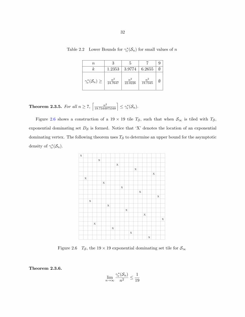
Theorem 2.3.5. For all n ≥ 7,⌈

n2

19.7344975348

⌉≤ γ∗e (Sn).

Figure 2.6 shows a construction of a 19 × 19 tile TS , such that when S∞ is tiled with TS ,

exponential dominating set DS is formed. Notice that ‘X’ denotes the location of an exponential

dominating vertex. The following theorem uses TS to determine an upper bound for the asymptotic

density of γ∗e (Sn).

X

X

X

X

X

X

X

X

X

X

X

X

X

X

X

X

X

X

X

Figure 2.6 TS , the 19× 19 exponential dominating set tile for S∞

Theorem 2.3.6.

limn→∞

γ∗e (Sn)

n2≤ 1

19

33

Proof. Let n = 19q + r, for some q, r ∈ Z and 0 ≤ r < 19. Let H denote the 19q × 19q subgrid of

Sn. Notice that we may tile H with the tiling scheme TS , as shown in Figure 2.6. Let DS be the

exponential dominating set that contains the 19q2 vertices used to tile H, as well as V (Sn \ H).

Therefore γ∗e (Sn) ≤ 19q2 + 38qr + r2, and we obtain the following asymptotic density:

limn→∞

γ∗e (Sn)

n2≤ lim

q→∞

19q2 + 38qr + r2

(19q + r)2≤ 1

19+ limq→∞

38qr + r2

(19q + r)2≤ 1

19,

as the limit equals zero.

Theorem 2.3.7. For n ≥ 19, γ∗e (Sn) ≤⌈n2

19

⌉+ o(n2).

Proof. This result follows directly from Theorem 2.3.6.

Similarly to Conjecture 2.1.4, we make the following conjecture.

Conjecture 2.3.8. For all n,⌈n2

23

⌉≤ γ∗e (Kn).

2.3.3 The n-dimensional hypercube

As Qn is not a grid graph, the method used to determine a value of k for Lemma 2.2.1 in

Remark 2.2.2 cannot be used to find the lower bound γ∗e (Qn). In order to determine such a lower

bound, a new method is used where distance properties of Qn are exploited.

Let D be a minimum exponential dominating set for Qn and let d ∈ D. Observe that for

u, v ∈ V (Qn), the length of the shortest uv path in Qn can be determined by the minimum number

of digits that must be changed to get from u to v. Then for all v ∈ V (Qn), we have that:

w∗(v, V (Qn)) =n∑i=0

(n

i

)(1

2

)i−1= 2

n∑i=0

(n

i

)(1

2

)i· 1n−i = 2

(1

2+ 1

)n= 2

(3

2

)n.

Thus it follows that m(Qn) = 2(32

)n.

In the following theorem, the decomposition in Figure 2.7 and value of m(Qn) are used to show

that(43

)n ≤ γ∗e (Qn) ≤ (√

2)n for large n.

Theorem 2.3.9. For all n ≥ 1,

⌈2n+3

24−n · 3n − 2n− 9

⌉≤ γ∗e (Qn) ≤ (

√2)n

34

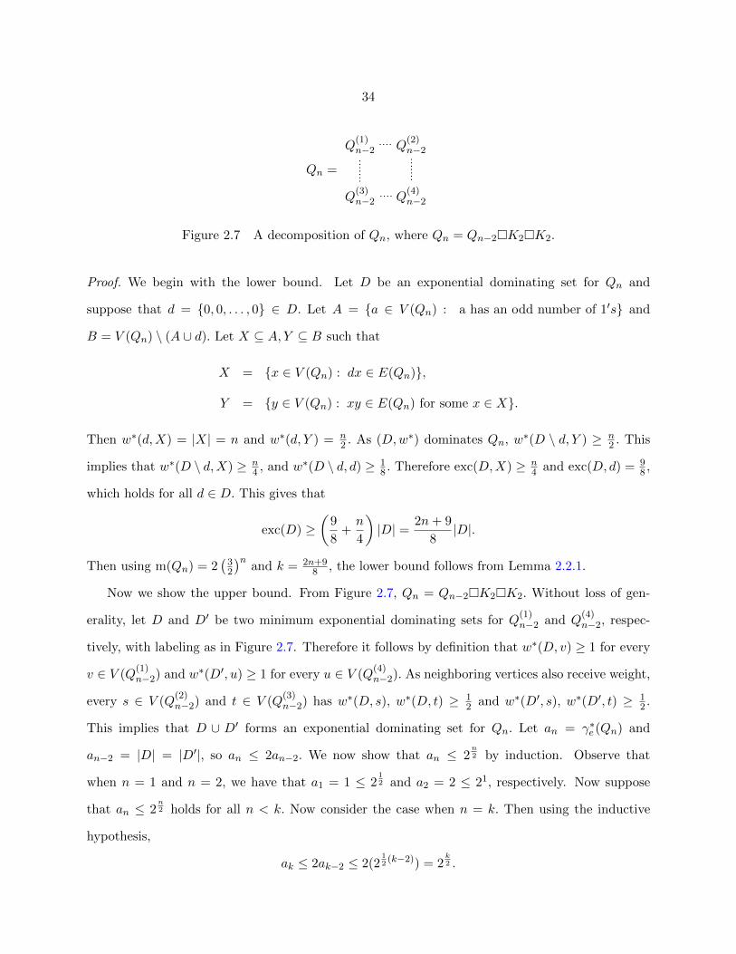
Qn =

Q(1)n−2 Q

(2)n−2

Q(4)n−2Q

(3)n−2

Figure 2.7 A decomposition of Qn, where Qn = Qn−2�K2�K2.

Proof. We begin with the lower bound. Let D be an exponential dominating set for Qn and

suppose that d = {0, 0, . . . , 0} ∈ D. Let A = {a ∈ V (Qn) : a has an odd number of 1′s} and

B = V (Qn) \ (A ∪ d). Let X ⊆ A, Y ⊆ B such that

X = {x ∈ V (Qn) : dx ∈ E(Qn)},

Y = {y ∈ V (Qn) : xy ∈ E(Qn) for some x ∈ X}.

Then w∗(d,X) = |X| = n and w∗(d, Y ) = n2 . As (D,w∗) dominates Qn, w

∗(D \ d, Y ) ≥ n2 . This

implies that w∗(D \ d,X) ≥ n4 , and w∗(D \ d, d) ≥ 1

8 . Therefore exc(D,X) ≥ n4 and exc(D, d) = 9

8 ,

which holds for all d ∈ D. This gives that

exc(D) ≥(

9

8+n

4

)|D| = 2n+ 9

8|D|.

Then using m(Qn) = 2(32

)nand k = 2n+9

8 , the lower bound follows from Lemma 2.2.1.

Now we show the upper bound. From Figure 2.7, Qn = Qn−2�K2�K2. Without loss of gen-

erality, let D and D′ be two minimum exponential dominating sets for Q(1)n−2 and Q

(4)n−2, respec-

tively, with labeling as in Figure 2.7. Therefore it follows by definition that w∗(D, v) ≥ 1 for every

v ∈ V (Q(1)n−2) and w∗(D′, u) ≥ 1 for every u ∈ V (Q

(4)n−2). As neighboring vertices also receive weight,

every s ∈ V (Q(2)n−2) and t ∈ V (Q

(3)n−2) has w∗(D, s), w∗(D, t) ≥ 1

2 and w∗(D′, s), w∗(D′, t) ≥ 12 .

This implies that D ∪ D′ forms an exponential dominating set for Qn. Let an = γ∗e (Qn) and

an−2 = |D| = |D′|, so an ≤ 2an−2. We now show that an ≤ 2n2 by induction. Observe that

when n = 1 and n = 2, we have that a1 = 1 ≤ 212 and a2 = 2 ≤ 21, respectively. Now suppose

that an ≤ 2n2 holds for all n < k. Now consider the case when n = k. Then using the inductive

hypothesis,

ak ≤ 2ak−2 ≤ 2(212(k−2)) = 2

k2 .

35

Therefore by induction, γ∗e (Qn) ≤ (√

2)n.

2.4 Acknowledgements

This research was supported in part by the National Science Foundation Award # 1719841.

We would like to thanks Dr. Leslie Hogben for her input on this paper.

2.5 Additional work

This section includes work that was not included in the paper A linear programming method

for exponential domination. For the sake of simplicity, we refer to porous exponential domination

as exponential domination. A potential way to increase the lower bound for γ∗e (Kn) and γ∗e (Sn)

described in Theorem 2.3.1 and Theorem 2.3.5, respectively, would be to add additional constraints

to Mixed Integer Linear Program 2.2.3. One such constraint would be to determine a global α for

all u ∈ V (G) such that w(Dα(u), u) ≥ 1.

Lemma 2.5.1. Let G be an infinite grid graph for which (D,w) is a dominating pair and suppose

that for every u ∈ V (G), there exists α such that w∗(Dα(u), u) ≥ 1. Then exc(D,u) > 0 for every

u ∈ V (G).

Proof. Suppose that for every u ∈ V (G), there exist an α such that w∗(Dα(u), u) ≥ 1. Consider

v ∈ V (G), and by assumption there exist α such that w∗(Dα(v), v) ≥ 1. As G is infinite, there

exists v′ ∈ V (G) and α′ such that w∗(Dα′(v′), v′) ≥ 1 and dist(v, v′) ≥ α+ α′. There then must be

at least one member d ∈ D such that d 6∈ Dα(v). Therefore it follows that

1 ≤ w∗(Dα(v), v) < w∗(Dα(v), v) + w∗(d, v).

Thus for all u ∈ V (G), exc(D,u) > 0.

Observe that the reverse of Lemma 2.5.1 does follow, if the additional assumptions that G is

connected and has infinite diameter. However without the added conditions, the result is unknown.

This leads to the following conjecture:

36

Conjecture 2.5.2. Let G be an infinite grid graph for which (D,w) is a dominating pair. If

exc(D,u) > 0 for every u ∈ V (G), then for every u ∈ V (G), there exists α such that w(Dα(u), u) ≥

1.

Results with a minimum distance amongst members of the exponential dominating set with

respect to the infinite grid graph G∞,∞ are examined in [1]. Let D be a set of vertices in G∞,∞,

then define the function In(v) =∑

w∈D\Bn−1(v)

(12

)dist(v,w)−1for any vertex v of G∞,∞ [1].

Lemma 2.5.3. [1] Given a set D of vertices in the infinite grid graph G∞,∞, if the minimum

distance between vertices in D is at least 5, then for any vertex v, In(v) ≤ 35n+36147·2n−4 .

Essentially Lemma 2.5.3 determined an upper bound on the potential weight a vertex receives

from members of the exponential dominating set whose distance from the vertex is at least n. With

restraints on the minimal distance between exponential dominating vertices, the smallest ball of

radius r that must contain an exponential dominating vertex was determined. These findings give

rise to another potential constraint to add to Mixed Integer Linear Program 2.2.3. In particular,

we focus on the infinite King Grid K∞.

Remark 2.5.4. Let v ∈ V (K∞) and let D be an exponential dominating set. If the minimum

distance between vertices in D is at least α, then there are at most |Sn(v)|α members of D ∩ Sn(v).

In the next lemma, we derive a formula to determine an upper bound for the weight that

v ∈ V (K∞) receives from D \ Bn−1(v) using An,n+2(v), with the restraint that the minimum

distance between members of the exponential dominating set is at least 4.

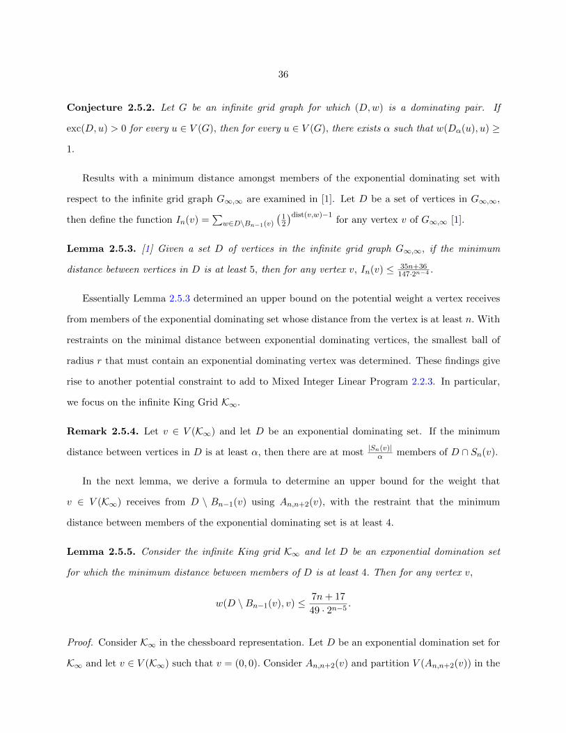
Lemma 2.5.5. Consider the infinite King grid K∞ and let D be an exponential domination set

for which the minimum distance between members of D is at least 4. Then for any vertex v,

w(D \Bn−1(v), v) ≤ 7n+ 17

49 · 2n−5.

Proof. Consider K∞ in the chessboard representation. Let D be an exponential domination set for

K∞ and let v ∈ V (K∞) such that v = (0, 0). Consider An,n+2(v) and partition V (An,n+2(v)) in the

37

v

5 5 5 5 5 5 5 5 5 5 5

5

5

5

5

5

5

5

5

5

55 5 5 5 5 5 5 5 55

5

5

5

5

5

5

5

5

5

5

6 6 6 6 6 6 6 6 6 6 6 6 6

6

6

6

6

6

6

6

6

6

6

6

6 6 6 6 6 6 6 6 6 6 6 6 6

6

6

6

6

6

6

6

6

6

6

6

6

6

7 7 7 7 7 7 7 7 7 7 7 7 7 7 7

7

7

7

7

7

7

7

7

7

7

7

7

7

7

7

7

7 7 7 7 7 7 7 7 7 7 7 7 7 7

7

7

7

7

7

7

7

7

7

7

7

7

7

7

7

7

7

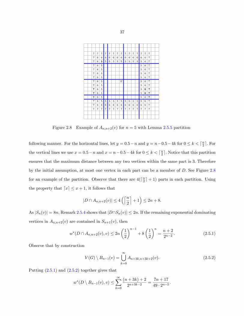
Figure 2.8 Example of An,n+2(v) for n = 5 with Lemma 2.5.5 partition

following manner. For the horizontal lines, let y = 0.5−n and y = n−0.5−4k for 0 ≤ k < dn2 e. For

the vertical lines we use x = 0.5−n and x = n−0.5−4k for 0 ≤ k < dn2 e. Notice that this partition

ensures that the maximum distance between any two vertices within the same part is 3. Therefore

by the initial assumption, at most one vertex in each part can be a member of D. See Figure 2.8

for an example of the partition. Observe that there are 4(dn2 e + 1) parts in each partition. Using

the property that dxe ≤ x+ 1, it follows that

|D ∩An,n+2(v)| ≤ 4(⌈n

2

⌉+ 1)≤ 2n+ 8.

As |Sn(v)| = 8n, Remark 2.5.4 shows that |D∩Sn(v)| ≤ 2n. If the remaining exponential dominating

vertices in An,n+2(v) are contained in Sn+1(v), then

w∗(D ∩An,n+2(v), v) ≤ 2n

(1

2

)n−1+ 8

(1

2

)n=n+ 2

2n−2. (2.5.1)

Observe that by construction

V (G) \Bn−1(v) =

∞⋃k=0

An+3k,n+3k+2(v). (2.5.2)

Putting (2.5.1) and (2.5.2) together gives that

w∗(D \Bn−1(v), v) ≤∞∑k=0

(n+ 3k) + 2

2n+3k−2 =7n+ 17

49 · 2n−5.

38

Table 2.3 shows the formula derived in Lemma 2.5.5 for small values of n. Notice that when

n = 6, the vertex v does not receive sufficient weight from D. This implies that there must be an

exponential dominating vertex contained in every ball of radius 5.

Table 2.3 Small values of n applied to Lemma 2.5.5

n 5 6 7

w∗(D \Bn−1(v), v) 1.06122 0.602041 0.336735

The following lemma mimics Lemma 2.5.5, with the added constraint that the minimum distance

between members of the exponential dominating set is at least 2.

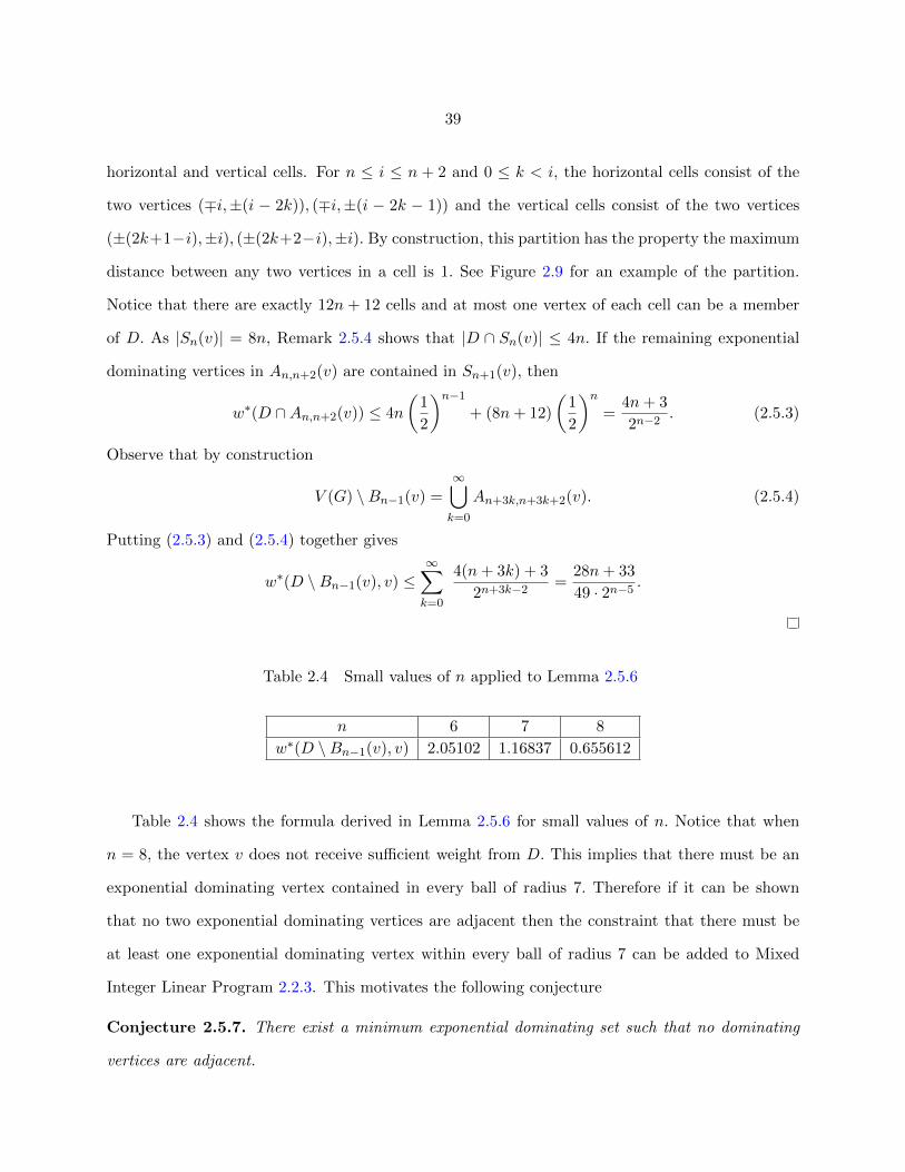
Lemma 2.5.6. Consider the infinite King grid K∞ and let D be an exponential domination set

for which the minimum distance between vertices in D is at least 2. Then for any vertex v,

w(D \Bn−1(v), v) ≤ 28n+ 33

49 · 2n−5.

5

5

5

5

5

5

5

5

5

5

5

5

5

5

5

5

5

5

5

5

5

5

5 5 5 5 5 5 5 5 5

5 5 5 5 5 5 5 5 5

4

4

4

4

4

4

4

4

4

4

4

4

4

4

4

4

4

44 4 4 4 4 4 4

4 4 4 4 4 4 4

3

3

3

3

3

3

3

3

3

3

3

3

3

3

3 3 3 3 3 3 3

3 3 3 3 3 3

v

Figure 2.9 Example of An,n+2(v) for n = 3 with Lemma 2.5.6 partition

Proof. Consider K∞ in the chessboard representation. Let D be an exponential domination set for

K∞ and let v ∈ V (K∞) such that v = (0, 0). Consider An,n+2(v) and partition V (An,n+2(v)) into

39

horizontal and vertical cells. For n ≤ i ≤ n + 2 and 0 ≤ k < i, the horizontal cells consist of the

two vertices (∓i,±(i − 2k)), (∓i,±(i − 2k − 1)) and the vertical cells consist of the two vertices

(±(2k+1−i),±i), (±(2k+2−i),±i). By construction, this partition has the property the maximum

distance between any two vertices in a cell is 1. See Figure 2.9 for an example of the partition.

Notice that there are exactly 12n + 12 cells and at most one vertex of each cell can be a member

of D. As |Sn(v)| = 8n, Remark 2.5.4 shows that |D ∩ Sn(v)| ≤ 4n. If the remaining exponential

dominating vertices in An,n+2(v) are contained in Sn+1(v), then

w∗(D ∩An,n+2(v)) ≤ 4n

(1

2

)n−1+ (8n+ 12)

(1

2

)n=

4n+ 3

2n−2. (2.5.3)

Observe that by construction

V (G) \Bn−1(v) =∞⋃k=0

An+3k,n+3k+2(v). (2.5.4)

Putting (2.5.3) and (2.5.4) together gives

w∗(D \Bn−1(v), v) ≤∞∑k=0

4(n+ 3k) + 3

2n+3k−2 =28n+ 33

49 · 2n−5.

Table 2.4 Small values of n applied to Lemma 2.5.6

n 6 7 8

w∗(D \Bn−1(v), v) 2.05102 1.16837 0.655612

Table 2.4 shows the formula derived in Lemma 2.5.6 for small values of n. Notice that when

n = 8, the vertex v does not receive sufficient weight from D. This implies that there must be an

exponential dominating vertex contained in every ball of radius 7. Therefore if it can be shown

that no two exponential dominating vertices are adjacent then the constraint that there must be

at least one exponential dominating vertex within every ball of radius 7 can be added to Mixed

Integer Linear Program 2.2.3. This motivates the following conjecture

Conjecture 2.5.7. There exist a minimum exponential dominating set such that no dominating

vertices are adjacent.

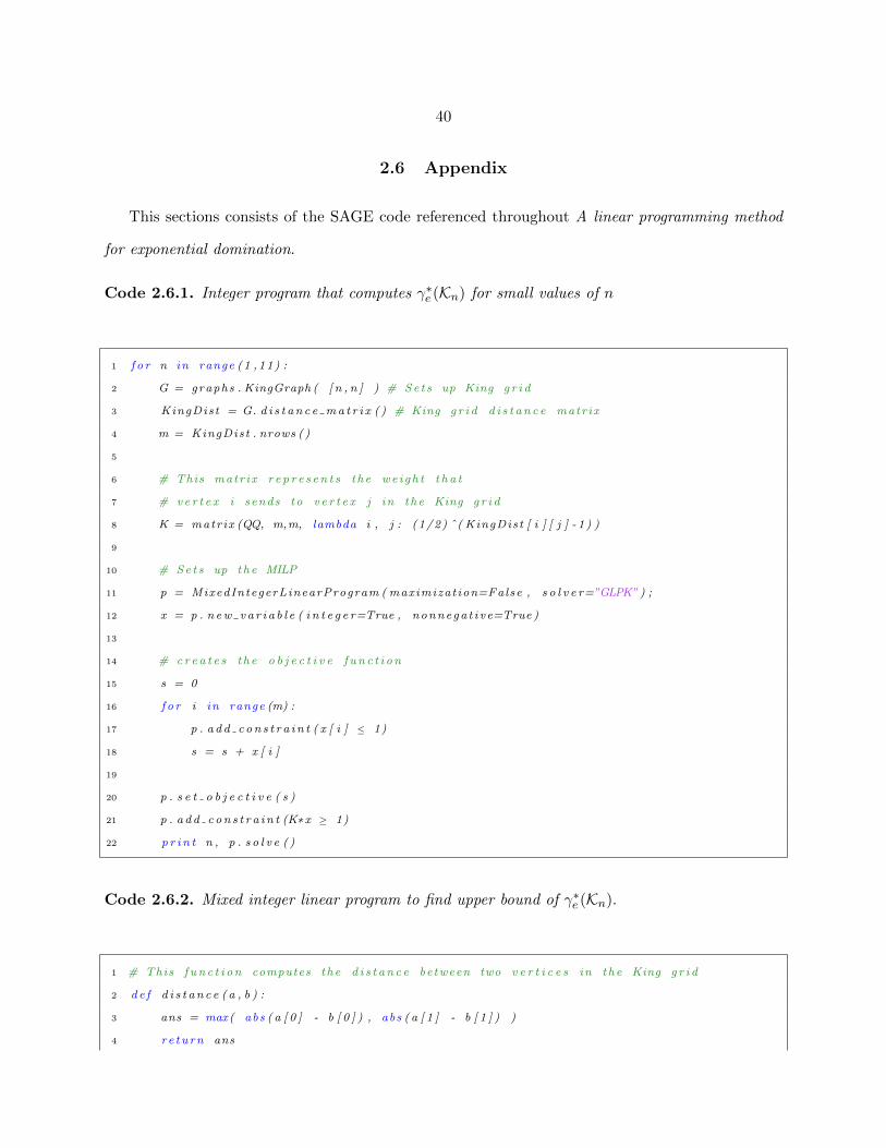
40

2.6 Appendix

This sections consists of the SAGE code referenced throughout A linear programming method

for exponential domination.

Code 2.6.1. Integer program that computes γ∗e (Kn) for small values of n

1 f o r n in range (1 ,11) :

2 G = graphs . KingGraph ( [ n , n ] ) # Se t s up King g r i d

3 KingDist = G. d i s t a n c e ma t r i x ( ) # King g r i d d i s t a n c e matr ix

4 m = KingDist . nrows ( )

5

6 # This matr ix r e p r e s e n t s t he we i gh t t h a t

7 # ve r t e x i sends to v e r t e x j in the King g r i d

8 K = matr ix (QQ, m,m, lambda i , j : (1/2) ˆ( KingDist [ i ] [ j ] - 1 ) )

9

10 # Se t s up the MILP

11 p = MixedIntegerLinearProgram ( maximizat ion=False , s o l v e r=”GLPK”) ;

12 x = p . n ew va r i a b l e ( i n t e g e r=True , nonnega t i ve=True )

13

14 # cr e a t e s t he o b j e c t i v e f un c t i on

15 s = 0

16 f o r i in range (m) :

17 p . a d d c on s t r a i n t ( x [ i ] ≤ 1)

18 s = s + x [ i ]

19

20 p . s e t o b j e c t i v e ( s )

21 p . a d d c on s t r a i n t (K∗x ≥ 1)

22 p r i n t n , p . s o l v e ( )

Code 2.6.2. Mixed integer linear program to find upper bound of γ∗e (Kn).

1 # This f un c t i on computes t he d i s t a n c e between two v e r t i c e s in the King g r i d

2 de f d i s t a n c e (a , b ) :

3 ans = max( abs ( a [ 0 ] - b [ 0 ] ) , abs ( a [ 1 ] - b [ 1 ] ) )

4 r e tu rn ans

41

5

6 # The Linear Program f o r the King g r i d

7 f o r n in range (3 , 13 , 2) :


9 x = p . n ew va r i a b l e ( r e a l=True , nonnega t i ve=True )

10 King = graphs . KingGraph ( [ n , n ] ) # Generated the nxn k ing g r i d

11 K = King . v e r t i c e s ( )

12

13 A = ze ro ma t r i x (RR, nˆ2 ,nˆ2) # Creates t he A matr ix f o r LP

14 f o r i in range (nˆ2) :

15 f o r j in range (nˆ2) :

16 A[ i , j ] = (1/2) ˆ d i s t an c e (K[ i ] , K[ j ] )

17

18 KingDist = z e r o ma t r i x (RR, nˆ2 ,nˆ2) # Creates t he d i s t a n c e matr ix f o r King g r i d



21 KingDist [ i , j ] = d i s t a n c e (K[ i ] ,K[ j ] )

22

23 b = [ 3 4 ]∗ nˆ2 # c r e a t e s t he b v e c t o r f o r King g r i d

24 f o r i in range (0 , nˆ2) :

25 i f divmod ( i , n) [ 1 ] != 0 and divmod ( i , n) [ 1 ] != n - 1 :

26 b [ i ] = 1+ (1/2) ˆ( KingDist [ ( nˆ2 -1) /2 , i ] - 1)

27

28 # Finds the inner v e r t i c e s o f King g r i d

29 l i s t =[ ]

30 f o r i in range (n , nˆ2 -n) :


32 l i s t = l i s t + [ i ]

33 #make the matr ix us ing on ly the rows t h a t are inner v e r t i c e s

34 c =A. matr i x f rom rows ( l i s t )

35 sum=0

36

37 one vec = [ 1 ] ∗ nˆ2

38 # Adds in the c on s t r a i n t t h a t 1≤ Ax

39 p . a d d c on s t r a i n t (A∗x ≥ one vec )

40 # Adds the c on s t r a i n t t h a t t he we i gh t o f t h e midd le v e r t e x i s 2

41 p . a d d c on s t r a i n t ( x [ ( nˆ2 -1) /2 ] == 2)

42 # Adds in the c on s t r a i n t t h a t Ax ≤ b

43 p . a d d c on s t r a i n t (A∗x ≤ b )

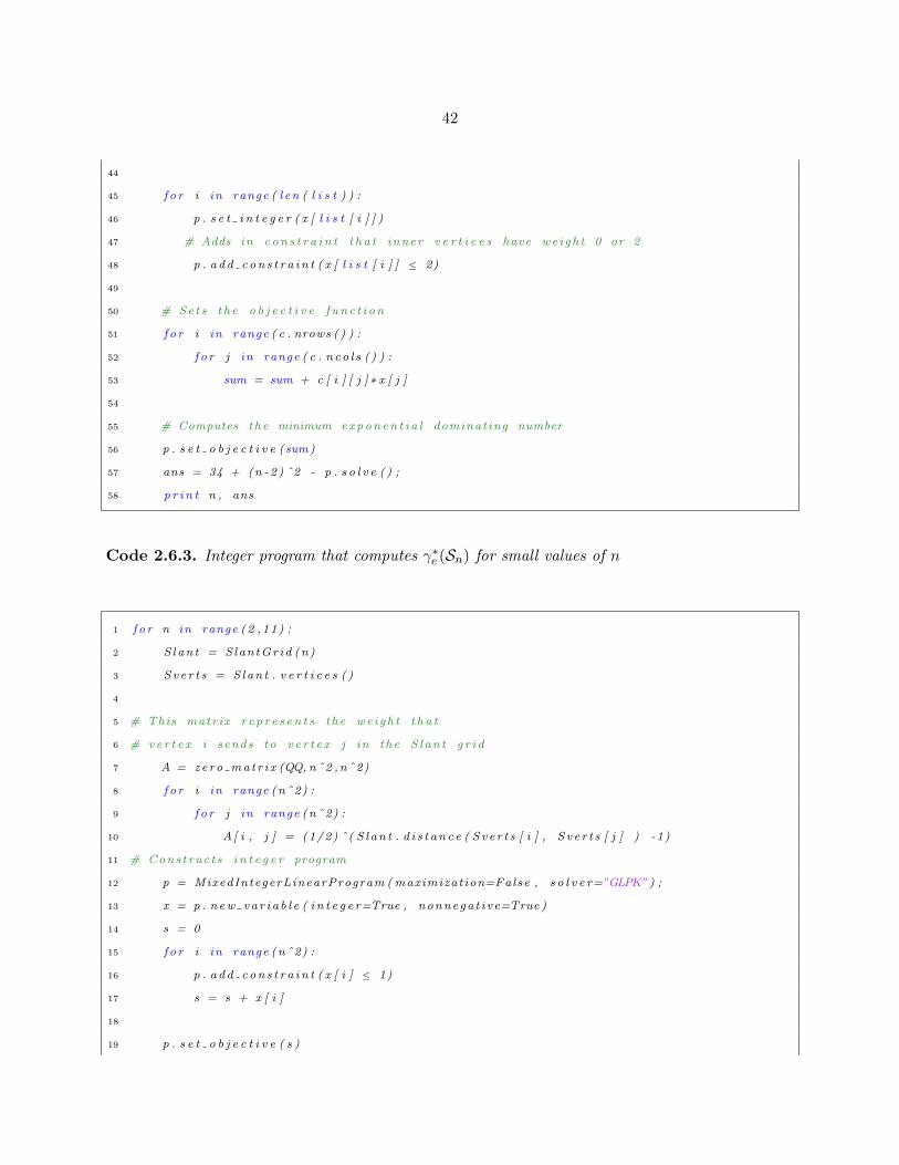
42

44

45 f o r i in range ( l en ( l i s t ) ) :

46 p . s e t i n t e g e r ( x [ l i s t [ i ] ] )

47 # Adds in c on s t r a i n t t h a t inner v e r t i c e s have we i gh t 0 or 2

48 p . a d d c on s t r a i n t ( x [ l i s t [ i ] ] ≤ 2)

49

50 # Se t s t he o b j e c t i v e f un c t i on

51 f o r i in range ( c . nrows ( ) ) :

52 f o r j in range ( c . n co l s ( ) ) :

53 sum = sum + c [ i ] [ j ]∗ x [ j ]

54

55 # Computes t he minimum expon en t i a l dominat ing number

56 p . s e t o b j e c t i v e (sum)

57 ans = 34 + (n -2 ) ˆ2 - p . s o l v e ( ) ;

58 p r i n t n , ans

Code 2.6.3. Integer program that computes γ∗e (Sn) for small values of n

1 f o r n in range (2 ,11) :

2 S l an t = S lan tGr id (n)

3 Sv e r t s = S l an t . v e r t i c e s ( )

4


6 # ve r t e x i sends to v e r t e x j in the S l an t g r i d

7 A = ze ro ma t r i x (QQ, nˆ2 ,nˆ2)



10 A[ i , j ] = (1/2) ˆ( S l an t . d i s t a n c e ( S v e r t s [ i ] , S v e r t s [ j ] ) -1)

11 # Cons t ruc t s i n t e g e r program



14 s = 0



17 s = s + x [ i ]

18

19 p . s e t o b j e c t i v e ( s )

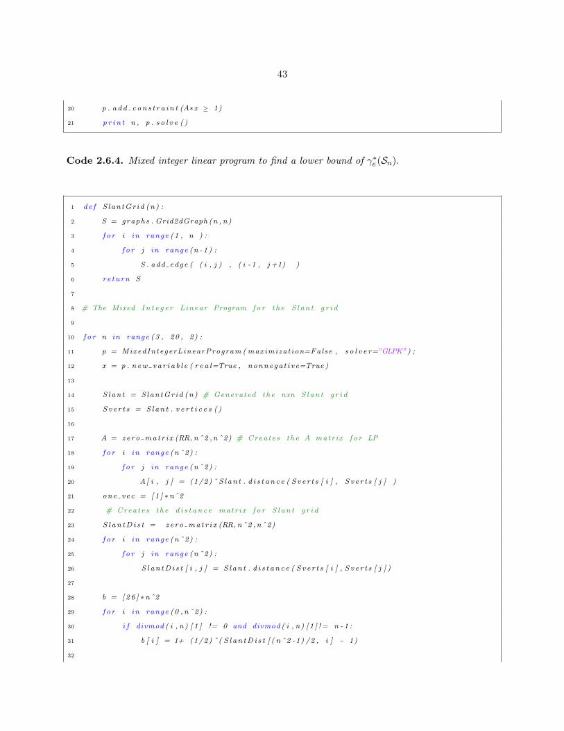
43

20 p . a d d c on s t r a i n t (A∗x ≥ 1)

21 p r i n t n , p . s o l v e ( )

Code 2.6.4. Mixed integer linear program to find a lower bound of γ∗e (Sn).

1 de f S lan tGr id (n) :

2 S = graphs . Grid2dGraph (n , n)

3 f o r i in range (1 , n ) :

4 f o r j in range (n -1 ) :

5 S . add edge ( ( i , j ) , ( i - 1 , j +1) )

6 r e tu rn S

7

8 # The Mixed I n t e g e r Linear Program f o r the S l an t g r i d

9

10 f o r n in range (3 , 20 , 2) :


12 x = p . n ew va r i a b l e ( r e a l=True , nonnega t i ve=True )

13

14 S l an t = S lan tGr id (n) # Generated the nxn S l an t g r i d

15 Sv e r t s = S l an t . v e r t i c e s ( )

16

17 A = ze ro ma t r i x (RR, nˆ2 ,nˆ2) # Creates t he A matr ix f o r LP



20 A[ i , j ] = (1/2) ˆ S l an t . d i s t a n c e ( S v e r t s [ i ] , S v e r t s [ j ] )

21 one vec = [ 1 ] ∗ nˆ2

22 # Creates t he d i s t an c e matr ix f o r S l an t g r i d

23 S l an tD i s t = z e r o ma t r i x (RR, nˆ2 ,nˆ2)



26 S l an tD i s t [ i , j ] = S l an t . d i s t a n c e ( S v e r t s [ i ] , S v e r t s [ j ] )

27

28 b = [ 2 6 ]∗ nˆ2

29 f o r i in range (0 , nˆ2) :


31 b [ i ] = 1+ (1/2) ˆ( S l an tD i s t [ ( nˆ2 -1) /2 , i ] - 1)

32

44

33 # Finds the inner v e r t i c e s o f S l an t g r i d

34 l i s t =[ ]

35 f o r i in range (n , nˆ2 -n) :


37 l i s t = l i s t + [ i ]

38 #make the matr ix us ing on ly the rows t h a t are inner v e r t i c e s

39 c =A. matr i x f rom rows ( l i s t )

40 sum=0

41

42 # Adds in the c on s t r a i n t t h a t 1≤ Ax

43 p . a d d c on s t r a i n t (A∗x ≥ one vec )

44 # Adds the c on s t r a i n t t h a t t he we i gh t o f t h e c en t e r v e r t e x i s 2

45 p . a d d c on s t r a i n t ( x [ ( nˆ2 -1) /2 ] == 2)

46 # Adds in the c on s t r a i n t t h a t Ax ≤ b

47 p . a d d c on s t r a i n t (A∗x ≤ b )

48

49 f o r i in range ( l en ( l i s t ) ) :

50 p . s e t i n t e g e r ( x [ l i s t [ i ] ] )

51 # Adds in c on s t r a i n t t h a t inner v e r t i c e s have we i gh t 0 ,1 , or 2

52 p . a d d c on s t r a i n t ( x [ l i s t [ i ] ] ≤ 2)

53

54 # Se t s t he o b j e c t i v e f un c t i on

55 f o r i in range ( c . nrows ( ) ) :

56 f o r j in range ( c . n co l s ( ) ) :

57 sum = sum + c [ i ] [ j ]∗ x [ j ]

58

59 # Computes t he minimum expon en t i a l dominat ing number

60 p . s e t o b j e c t i v e (sum)

61 ans = 26 + (n -2 ) ˆ2 - p . s o l v e ( ) ;

62 p r i n t n , ans , p . s o l v e ( ) - (n - 2 ) ˆ2

Code 2.6.5. Integer program that computes γ∗e (Qn) for small values of n

1 f o r m in range (1 , 8) :

2 g = graphs . CubeGraph (m)

3 M = g . d i s t a n c e ma t r i x ( )

4

45

5 # s e t s up the i n t e g e r program


7 n = M. nrows ( )

8


10 # ve r t e x i sends to v e r t e x j in the hypercube

11 K = matr ix (QQ, n , n , lambda i , j : (1/2) ˆ(M[ i ] [ j ] - 1 ) )


13 s = 0

14 f o r i in range (n) :


16 s = s + x [ i ]

17

18 # s e t s t he o b j e c t i v e f un c t i on and c o n s t r a i n t s

19 p . s e t o b j e c t i v e ( s )

20 p . a d d c on s t r a i n t (K∗x ≥ 1)

21 p r i n t m, p . s o l v e ( )

2.7 Bibliography



[2] Aysun Aytac and Betul Atay. On exponential domination of some graphs. Nonlinear Dyn.

Syst. Theory, 16(1):12–19, 2016.





[5] Chassidy Bozeman, Joshua Carlson, Michael Dairyko, Derek Young, and Michael Young. Lower

bounds for the exponential domination number of Cm × Cn. arXiv:1803.01933, 2018.

46









domination, and porous exponential domination. Discrete Optimization, 23:81–92, 2017.

47

CHAPTER 3. ON EXPONENTIAL DOMINATION OF THE

GENERALIZED CIRCULANT GRAPH

Modified from of a submitted paper

Michael Dairyko1 and Michael Young

Abstract

For a graph G, we consider D ⊂ V (G) to be a porous exponential dominating set if 1 ≤∑

d∈D

(2)1−dist(d,v) for every v ∈ V (G), where dist(d, v) denotes the length of the smallest dv path.

Similarly, D ⊂ V (G) is a non-porous exponential dominating set is 1 ≤∑

d∈D (2)1−dist(d,v) for

every v ∈ V (G), where dist(d, v) represents the length of the shortest dv path with no internal

vertices in D. The porous and non-porous exponential dominating number of G, denoted γ∗e (G)

and γe(G), are the minimum cardinality of a porous and non-porous exponential dominating set,

respectively. The consecutive circulant graph, Cn,[`], is the set of n vertices such that vertex v is

adjacent to v ± i mod n for each i ∈ [`]. In this paper we show γe(Cn,[`]) = γ∗e (Cn,[`]) =⌈

n3`+1

⌉.

AMS 2010 Subject Classification: Primary 05C69; Secondary 05C12

Keywords: domination, generalized circulant graph, exponential domination, porous exponen-

tial domination

3.1 Introduction

Domination in graphs is a well studied area within graph theory. For a graph G, we consider D ⊂

V (G) to be a dominating set if every member of V (G)\D is adjacent to at least one member of D.

The domination number of G, denoted γ(G), is the minimum cardinality of a dominating set. Define

w : V (G)× V (G)→ R to be a weight function of G. For u, v ∈ V (G), we say that u assigns weight

1Primary Researcher and Author.

48

w(u, v) to v. Denote the weight assigned by a set of vertices D to v as w(D, v) :=∑

d∈D w(d, v),

and similarly, the weight assigned by d ∈ D to H ⊂ V (G) as w(d,H) :=∑

h∈H w(d, h). The pair

(D,w) dominates G if w(D, v) ≥ 1 for every v ∈ V (G). In the context of domination, the pair

(D,w) dominates G where D is a dominating set and w is the following function:

w(u, v) =

1 if u ∈ D and uv ∈ E(G)

0 otherwise.

A variant of domination, called exponential domination, was first introduced in [5]. Their

motivation was to create a framework for a particular type of distance domination, one that would

better model real world situations in which the influence of a selected vertex on other vertices

decreases exponentially as their distance increases. There are two types of exponential domination;

non-porous and porous. In non-porous exponential domination, exponential dominating vertices

obstruct the influence of each other, whereas there is no such obstruction in porous exponential

domination. More formally, the weight function for non-porous exponential domination is

w(u, v) =

(1

2

)dist(u,v)−1,

where dist(u, v) represents the length of the shortest uv path that does not contain any internal

vertices that are in the non-porous exponential dominating set. The non-porous exponential dom-

ination number of G, denoted by γe(G), is the cardinality of a minimum non-porous exponential

dominating set. The weight function for porous exponential domination is

w∗(u, v) =

(1

2

)dist(u,v)−1,

where dist(u, v) represents the length of the shortest uv path. The porous exponential domination

number of G, denoted by γ∗e (G), is the cardinality of a minimum porous exponential dominating

set.

Notice that exponential domination differs from the other variants of domination discussed in [6]

due to the global influence exponential dominating vertices have on V (G), whereas the dominating

vertices of the variants of domination have a more local influence. The relatively few results

49

[1, 2, 3, 4, 5, 7, 8] in this area has been attributed to the difficulty of working within the global

nature of exponential domination. On relating exponential domination to domination, it is known

that [5]

γ∗e (G) ≤ γe(G) ≤ γ(G). (3.1.1)

Let [n] = {1, 2, . . . , n}. The consecutive circulant graph, Cn,[`], is the set of n vertices such that

vertex v is adjacent to vertex v ± i mod n for each i ∈ [`]. Notice that Cn,[1] is equivalent to Cn

and Cn,[bn2 c] is equivalent to the complete graph Kn. The following proposition gives an explicit

formula for γe(Cn).

Proposition 3.1.1. [5] For every integer n ≥ 3,

γe(Cn) =

2 if n = 4⌈n4

⌉if n 6= 4.

No such formula has been determined for γ∗e (Cn). In this paper, we show that that the porous

and non-porous exponential domination number of Cn,[`] are equivalent. Furthermore, in Theorem

3.1.2 when ` = 1 and m ≥ 2, our results align with Proposition 3.1.1 and fills the gap to γ∗e (Cn).

For the sake of simplicity, we will now refer to porous exponential domination as exponential

domination, unless stated otherwise.

We still need a few more definitions and notation. Let H be the Hamiltonian cycle of Cn,[`],

where the vertices v, v + 1 mod n form an edge. Label the vertices of Cn,[`] in the order of H as

VH = {0, 1, . . . , n− 1}. For 0 ≤ i, j ≤ n− 1, we denote distH(i, j) to be the length of the shortest

path from i to j on H. See Figure 3.1 for an illustration of C8,[2], with the defined labeling. With

respect to V (Cn,[`]), denote the interval [i, j] as the set of increasing consecutive integers modulo n

from i to j. Let I =⋃m−1i=0 Ii be the consecutive partition around H. For any exponential dominating

set D, let fk(D, I) := |Ik ∩D|. Also define z(D, I) := {i : fi(D, I) = 0}, Z(D, I) := |z(D, I)|, and

f∗(D, I) := max0≤i≤m−1

fi(D, I).

Our main result is the following theorem, whose proof is shown in Section 3.2.2.

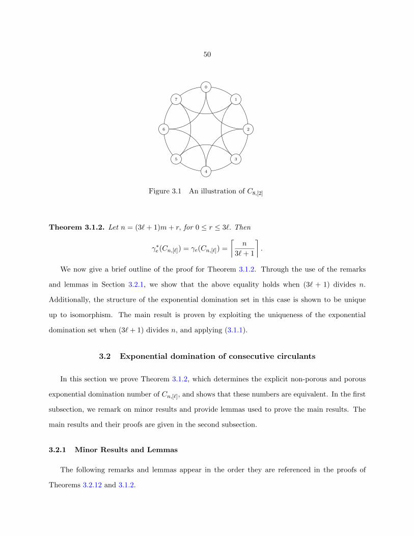
50

2

1

0

7

6

5

4

3

Figure 3.1 An illustration of C8,[2]

Theorem 3.1.2. Let n = (3`+ 1)m+ r, for 0 ≤ r ≤ 3`. Then

γ∗e (Cn,[`]) = γe(Cn,[`]) =

⌈n

3`+ 1

⌉.

We now give a brief outline of the proof for Theorem 3.1.2. Through the use of the remarks

and lemmas in Section 3.2.1, we show that the above equality holds when (3` + 1) divides n.

Additionally, the structure of the exponential domination set in this case is shown to be unique

up to isomorphism. The main result is proven by exploiting the uniqueness of the exponential

domination set when (3`+ 1) divides n, and applying (3.1.1).

3.2 Exponential domination of consecutive circulants

In this section we prove Theorem 3.1.2, which determines the explicit non-porous and porous

exponential domination number of Cn,[`], and shows that these numbers are equivalent. In the first

subsection, we remark on minor results and provide lemmas used to prove the main results. The

main results and their proofs are given in the second subsection.

3.2.1 Minor Results and Lemmas

The following remarks and lemmas appear in the order they are referenced in the proofs of

Theorems 3.2.12 and 3.1.2.

51

Remark 3.2.1. Consider u, v ∈ V (Cn,[`]). Throughout the paper, there will be a need to refer to

dist(u, v). Notice that,

dist(u, v) =

⌈distH(u, v)

`

⌉.

Remark 3.2.2. Suppose that [a, b] is an interval on H such that a < b and distH(a, b) ≤ 3` + 1.

For notational simplicity, consider the interval [0, 3` + 1]. Then 0 and 3` + 1 dominates [1, `] and

[2`+1, 3`], respectively, and both 0 and 3`+1 contribute weight 12 to [`+1, 2`]. Therefore [0, 3`+1]

is exponentially dominated by 0 and 3`+ 1. This shows that a, b exponentially dominates [a, b].

Remark 3.2.3. For n = (3`+ 1)m, with m ≥ 2, let D be a minimum exponential dominating set

for Cn,[`]. Fix vertex i ∈ VH and construct set D∗ = {i+(3`+1)t mod n : 0 ≤ t ≤ m−1}. Through

the application of Remark 3.2.2, D∗ forms an exponential dominating set for which |D| ≤ |D∗| = m.

Remark 3.2.4. Let D be a minimum exponential dominating set for Cn,[`]. From Remark 3.2.3,

we have that |D| ≤ m. Therefore, for every interval Ik with fk(D) > 1, there must exist fk(d)− 1

distinct intervals that contain no members of D. This shows that∑m−1

k=0 fk(D) ≤ m.

In many of the cases for the proof of Theorem 3.1.2, an exponential dominating set D can be

reduced to having at least one interval with no members of D and the remaining intervals with

exactly one member of D. The following lemma gives results on D in this situation.

Lemma 3.2.5. Let D ⊂ V (Cn,[`]) and I be a partition such that I =⋃m−1i=0 Ii, where Ii = [(3` +

1)i, (3`+ 1)i+ 3`] such that f∗(D, I) = 1 and Z(D, I) ≥ 1. Let di := Ii ∩D for 0 ≤ i ≤ m− 1, and

consider z ∈ z(D, I). Then,

(i) w∗(D, (3`+ 1)z + `) < 67 and w∗(D, (3`+ 1)z + 2`) < 6

7 ,

(ii) w∗(D \ dk, (3`+ 1)z + `) < 1728 and w∗(D \ dk, (3`+ 1)z + 2`) < 5

14 , for k ≡ z + 1 mod m,

(iii) w∗(D \ dk, (3`+ 1)z + `) < 514 and w∗(D \ dk, (3`+ 1)z + 2`) < 17

28 , for k ≡ z − 1 mod m.

(iv) w∗(D \ dk, (3`+ 1)z + `) < 377448 and w∗(D \ dk, (3`+ 1)z + 2`) < 185

224 , for k ≡ z + 2 mod m,

(v) w∗(D \ dk, (3`+ 1)z + `) < 185224 and w∗(D \ dk, (3`+ 1)z + 2`) < 377

448 , for k ≡ z − 2 mod m.

52

Proof. Let I be the partition such that I =⋃m−1i=0 Ii, where Ii = [(3`+ 1)i, (3`+ 1)i+ 3`]. For the

sake of simplicity, let f(D) = f(D, I), f∗(D) = f∗(D, I), z(D) = z(D, I), and Z(D) = Z(D, I).

Without loss of generality, suppose that 0 ∈ z(D). Then the interval I0 has f0(D) = 0. Among such

D, choose D′ to maximize w∗(D′, 2`) and let k0 =⌊m2

⌋. Then the choice of D′ implies that

Ik ∩D′ =

(3`+ 1)k for k ≤ k0

(3`+ 1)k + 3` for k > k0.

Consider k ≤ k0 and notice that distH(2`, (3`+ 1)k) = (3`+ 1)k − 2` = (3k − 2)`+ k. By Remark

3.2.1,

dist(2`, (3`+ 1)k) =

⌈(3k − 2)`+ k

`

⌉= 3k − 2 +

⌈k

`

⌉. (3.2.1)

Using the fact that 1 ≤⌈k`

⌉, it follows that

k0∑k=1

w∗(Ik ∩D′, 2`) =

k0∑k=1

(1

2

)dist(2`,(3`+1)k)−1<

∞∑k=1

(1

2

)dist(2`,(3`+1)k)−1

(3.2.2)

=

∞∑k=1

(1

2

)3k−3+d k` e≤

∞∑k=1

(1

2

)3k−2

(3.2.3)

=1

2

∞∑t=0

(1

2

)3t

=4

7.

Now consider k > k0 and let k′ = m− k. Then with respect to VH ,

distH(2`, (3`+ 1)k + 3`) = distH((3`+ 1)m+ 2`, (3`+ 1)k + 3`)

= (3`+ 1)m+ 2`− (3`+ 1)k − 3`

= (3k′ − 1)`+ k′.

Again, applying Remark 3.2.1 gives,

dist(2`, (3`+ 1)k + 3`) =

⌈(3k′ − 1)`+ k′

`

⌉= 3k′ − 1 +

⌈k′

`

⌉. (3.2.4)

53

Notice since k and k′ are counters, (3.2.1) and (3.2.4) only differ by `. Furthermore, summing from

k = k0 + 1 to m − 1 is the same as summing k′ from 1 to m − k0 − 1, which equals k0 or k0 − 1.

Therefore we have shown that

w∗(D, 2`) ≤ w∗(D′, 2`) <3

2

k0∑k=1

w∗(Ik ∩D′, 2`) <6

7.

Applying a symmetric argument gives that w∗(D, `) < 67 , and (i) has been established. Let d′k :=

Ik ∩D′ and observe that w∗(D \ dk, `) ≤ w∗(D′ \ d′k, `) and w∗(D \ dk, 2`) ≤ w∗(D′ \ d′k, 2`). Notice

that by construction, d′1 = 3`+ 1 and d′2 = 6`+ 2. Then applying

distH(d′1, `) = 3`+ 1− ` = 2`+ 1,

distH(d′1, 2`) = 3`+ 1− 2` = `+ 1,

distH(d′2, `) = 6`+ 2− ` = 5`+ 2,

distH(d′2, 2`) = 6`+ 2− 2` = 4`+ 2,

with Remark 3.2.1, and the fact that 1 =⌈1`

⌉and 1 ≤

⌈2`

⌉≤ 2 yields

w∗(d′1, `) =(12

)dist(3`+1,`)−1=

(12

)1+d 1` e = 14 ,

w∗(d′1, 2`) =(12

)dist(3`+1,2`)−1=

(12

)d 1` e = 12

164 ≤ w∗(d′2, `) =

(12

)dist(6`+2,`)−1=

(12

)4+d 2` e ≤ 132 ,

132 ≤ w∗(d′2, 2`) =

(12

)dist(6`+2,2`)−1=

(12

)3+d 2` e ≤ 116 .

Therefore,

w∗(D \ d1, `) ≤ w∗(D′ \ d′1, `) < 67 − w∗(d′1, `) = 17

28 ,

w∗(D \ d1, 2`) ≤ w∗(D′ \ d′1, 2`) < 67 − w∗(d′1, 2`) = 5

14 ,

w∗(D \ d2, `) ≤ w∗(D′ \ d′2, `) < 67 − w∗(d′2, `) = 377

448 ,

w∗(D \ d2, 2`) ≤ w∗(D′ \ d′2, 2`) < 67 − w∗(d′2, 2`) = 185

224 .

54

Therefore (ii) and (iv) have been verified. Observe that (iii) and (v) are a symmetric argument to

(ii) and (iv), respectively.

Given an exponential dominating set D, the following algorithm details the process in how

to construct a new exponential dominating set of the same size. With respect to D, this new

exponential dominating set has less intervals that contain no exponential dominating vertices, or

has less exponential dominating vertices contained in each interval.

Algorithm 3.2.6. Consider D, an exponential dominating set for Cn,[`], and the partition I such

that I =⋃m−1i=0 Ii, where Ii = [(3`+1)i, (3`+1)i+3`]. For the sake of simplicity, let f(D) = f(D, I),

f∗(D) = f∗(D, I) and Z(D) = Z(D, I). Suppose that 3 ≤ f∗(D). Observe that by Remark 3.2.4,

Z(D) ≥ 2. Without loss of generality, assume that for 0 < b ≤ m, the intervals I0 and Ib have

that f0(D) = fb(D) = 0. Find the interval Ia such that a = min{1, 2, . . . , b − 1} and fa(D) ≥ 3.

Furthermore, assume that the remaining 0 < i < b have fi(D) ≥ 1. Without loss of generality

suppose that a ≤ b− a (use a reflection if necessary). Observe that there are at least f∗(D) + b− 2

exponential dominating vertices contained in [0, (3`+1)b+3`]. We identify the three closest members

of Ia∩D to (3`+ 1)a+ 2`, and the closest member to (3`+ 1)i+ 2` within Ii∩D for 1 ≤ i 6= a ≤ b,

to be defined as P = {d0, d1, . . . , db} for which

di ∈

Ii+1 ∩D if 0 ≤ i ≤ a− 2

Ia ∩D if a− 1 ≤ i ≤ a+ 1

Ii−1 ∩D if a+ 2 ≤ i ≤ b.

Then define S = {s0, s1, . . . , sb}, such that st = (3`+ 1)t+ 2`, and output the set D′ = (D \P )∪S.

Lemma 3.2.7. Given an exponential dominating set D ⊂ V (Cn,[`]), and the partition I so that

I =⋃m−1i=0 Ii, where Ii = [(3` + 1)i, (3` + 1)i + 3`] and 3 ≤ f∗(D, I) ≤ 3` + 1, Algorithm 3.2.6

outputs the exponential dominating set D′ such that |D| = |D′|, Z(D′, I) = Z(D, I) − 2, and

f∗(D, I)− 2 ≤ f∗(D′, I) ≤ f∗(D, I).

Proof. For the sake of simplicity, let f(D) = f(D, I), f∗(D) = f∗(D, I) and Z(D) = Z(D, I).

Notice that by construction, |D| = |D′| and distH(si, si+1) = 3` + 1 for each consecutive pair

55

si, si+1 ∈ S. Through applications of Remark 3.2.2, all the vertices in [s0, sb] are exponentially

dominated by vertices of S. Let V ′ = V (Cn,[`]) \ [s0, sb]. We define VL = {v ∈ V ′ : distH(v, da+1) ≤

distH(v, da+1 + 1)} and VR = V ′ \ VL. There are four cases:

1. Consider the case when v ∈ VL. Then w∗(di, v) ≥ w∗(di+1, v) for 0 ≤ i ≤ b− 1. By construc-

tion, w∗(da−2, v) + w∗(da−1, v) ≤ 2w∗(da−2, v) ≤ w∗(sa−2, v) and w∗(da, v) + w∗(da+1, v) ≤

2w∗(da, v) ≤ w∗(sa−1, v). Additionally, w∗(di, v) ≤ w∗(si, v) for 0 ≤ i ≤ a− 3 and w∗(di, v) ≤

w∗(si−2, v), for a + 2 ≤ i ≤ b. Figure 3.2 visually shows that w∗(P ∩D, v) < w∗(S, v). Then

putting it together gives that

w∗(P ∩D, v) =a−3∑k=0

w∗(dk, v) +a−1∑

k=a−2w∗(dk, v) +

a+1∑k=a

w∗(dk, v) +b∑

k=a+2

w∗(dk, v)

<a−3∑k=0

w∗(sk, v) + w∗(sa−2, v) + w∗(sa−1, v) +b−2∑k=a

w∗(sk, v)

< w∗(S, v).

I0 I1 I2 I3 I4 I5 I6 I7

∅ d0 d1 d2, d3, d4 d5 d6 d7 ∅

s0 s1 s2 s3 s4 s5 s6 s7

Figure 3.2 Illustration of Case 1 with a = 3, b = 7

2. Consider the case when v ∈ VR such that w∗(di, v) ≤ w∗(di+1, v) for 0 ≤ i ≤ b − 1. Then

distH(da+1, sa+1) ≥ 2`+1, which implies that∑a+1

k=a−1w∗(dk, v) ≤ 3w∗(da+1, v) < w∗(sa+1, v).

Also by construction, w∗(di, v) ≤ w∗(si+2, v), for 0 ≤ i ≤ a− 2 and w∗(di, v) ≤ w∗(si, v), for

a+ 2 ≤ i ≤ b. Figure 3.3 visually shows that w∗(P ∩D, v) < w∗(S, v). Then it follows that

w∗(P ∩D, v) =a−2∑k=0

w∗(dk, v) +a+1∑

k=a−1w∗(dk, v) +

b∑k=a+2

w∗(dk, v)

<a∑k=2

w∗(sk, v) + w∗(sa+1, v) +b∑

k=a+2

w∗(sk, v)

< w∗(S, v).

56

I0 I1 I2 I3 I4 I5 I6 I7

∅ d0 d1 d2, d3, d4 d5 d6 d7 ∅

s0 s1 s2 s3 s4 s5 s6 s7

Figure 3.3 Illustration of Case 2 with a = 3, b = 7.

3. Consider the case when v ∈ VR such that w∗(di, v) ≥ w∗(di+1, v) for 0 ≤ i < a and w∗(di, v) ≤

w∗(di+1, v) for a + 1 ≤ i < b − 1. By construction, w∗(da−1, v) + w∗(da, v) ≤ 2w∗(da−1, v) ≤

w∗(sa−1, v). Additionally we have that w∗(di, v) ≤ w∗(si, v), for 0 ≤ i 6= a− 1, a ≤ b. Figure

3.4 visually shows that w∗(P ∩D, v) < w∗(S, v). Putting it together gives

w∗(P ∩D, v) =a−2∑k=0

w∗(dk, v) +a∑

k=a−1w∗(dk, v) +

b∑k=a+1

w∗(dk, v)

<

a−2∑k=0

w∗(sk, v) + w∗(sa−1, v) +

b∑k=a+1

w∗(sk, v)

< w∗(S, v).

I0 I1 I2 I3 I4 I5 I6 I7

∅ d0 d1 d2, d3, d4 d5 d6 d7 ∅

s0 s1 s2 s3 s4 s5 s6 s7


4. Consider the case when v ∈ VR such that w∗(di, v) ≥ w∗(di+1, v) for 0 ≤ i < a − 1 and

w∗(di, v) ≤ w∗(di+1, v) for a ≤ i < b − 1. By construction, w∗(da, v) + w∗(da+1, v) ≤

2w∗(da+1, v) ≤ w∗(sa+1, v). Additionally we have that w∗(di, v) ≤ w∗(si, v), for 0 ≤ i 6=

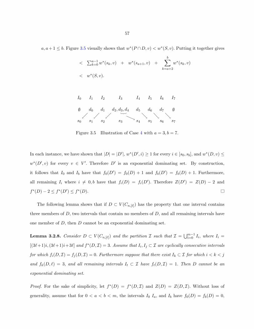
57

a, a+ 1 ≤ b. Figure 3.5 visually shows that w∗(P ∩D, v) < w∗(S, v). Putting it together gives

<∑a−1

k=0w∗(sk, v) + w∗(sa+1, v) +

b∑k=a+2

w∗(sk, v)

< w∗(S, v).

I0 I1 I2 I3 I4 I5 I6 I7

∅ d0 d1 d2, d3, d4 d5 d6 d7 ∅

s0 s1 s2 s3 s4 s5 s6 s7


In each instance, we have shown that |D| = |D′|, w∗(D′, i) ≥ 1 for every i ∈ [s0, sb], and w∗(D, v) ≤

w∗(D′, v) for every v ∈ V ′. Therefore D′ is an exponential dominating set. By construction,

it follows that I0 and Ib have that f0(D′) = f0(D) + 1 and fb(D

′) = fb(D) + 1. Furthermore,

all remaining Ii where i 6= 0, b have that fi(D) = fi(D′). Therefore Z(D′) = Z(D) − 2 and

f∗(D)− 2 ≤ f∗(D′) ≤ f∗(D).

The following lemma shows that if D ⊂ V (Cn,[`]) has the property that one interval contains

three members of D, two intervals that contain no members of D, and all remaining intervals have

one member of D, then D cannot be an exponential dominating set.

Lemma 3.2.8. Consider D ⊂ V (Cn,[`]) and the partition I such that I =⋃m−1i=0 Ii, where Ii =

[(3`+1)i, (3`+1)i+3`] and f∗(D, I) = 3. Assume that Ii, Ij ⊂ I are cyclically consecutive intervals

for which fi(D, I) = fj(D, I) = 0. Furthermore suppose that there exist Ik ⊂ I for which i < k < j

and fk(D, `) = 3, and all remaining intervals It ⊂ I have ft(D, I) = 1. Then D cannot be an


Proof. For the sake of simplicity, let f∗(D) = f∗(D, I) and Z(D) = Z(D, I). Without loss of

generality, assume that for 0 < a < b < m, the intervals I0 Ia, and Ib have f0(D) = fb(D) = 0,

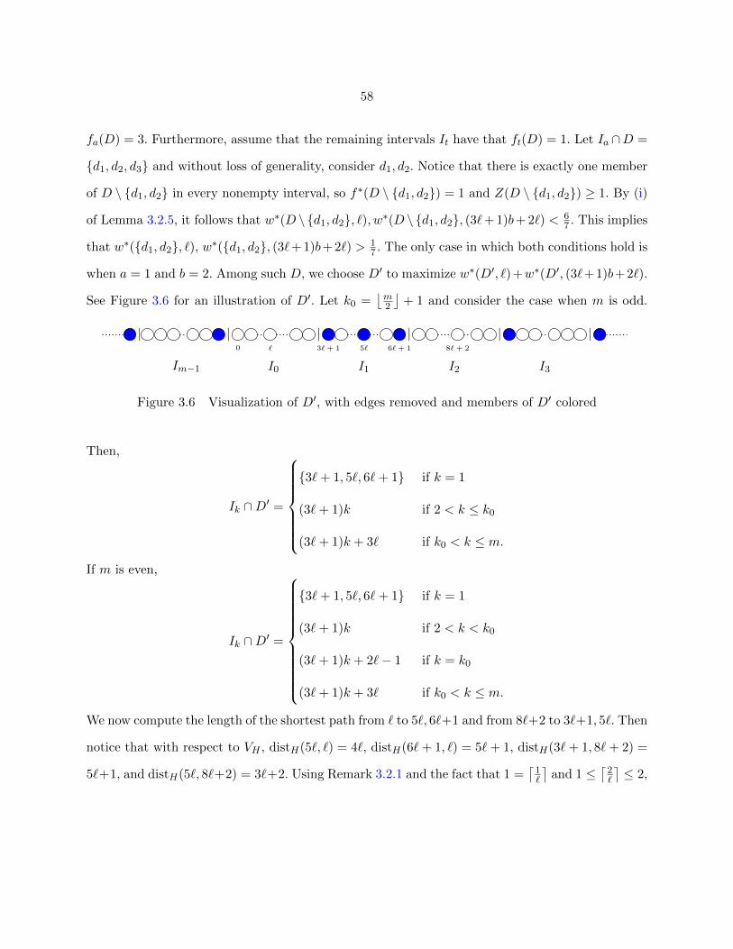
58

fa(D) = 3. Furthermore, assume that the remaining intervals It have that ft(D) = 1. Let Ia ∩D =

{d1, d2, d3} and without loss of generality, consider d1, d2. Notice that there is exactly one member

of D \ {d1, d2} in every nonempty interval, so f∗(D \ {d1, d2}) = 1 and Z(D \ {d1, d2}) ≥ 1. By (i)

of Lemma 3.2.5, it follows that w∗(D \ {d1, d2}, `), w∗(D \ {d1, d2}, (3`+ 1)b+ 2`) < 67 . This implies

that w∗({d1, d2}, `), w∗({d1, d2}, (3`+ 1)b+ 2`) > 17 . The only case in which both conditions hold is

when a = 1 and b = 2. Among such D, we choose D′ to maximize w∗(D′, `)+w∗(D′, (3`+1)b+2`).

See Figure 3.6 for an illustration of D′. Let k0 =⌊m2

⌋+ 1 and consider the case when m is odd.

|

Im−1

|

I0

0 `

|

I1

3` + 1 5` 6` + 1

|

I2

8` + 2

|

I3

|

Figure 3.6 Visualization of D′, with edges removed and members of D′ colored

Then,

Ik ∩D′ =

{3`+ 1, 5`, 6`+ 1} if k = 1

(3`+ 1)k if 2 < k ≤ k0

(3`+ 1)k + 3` if k0 < k ≤ m.

If m is even,

Ik ∩D′ =

{3`+ 1, 5`, 6`+ 1} if k = 1

(3`+ 1)k if 2 < k < k0

(3`+ 1)k + 2`− 1 if k = k0

(3`+ 1)k + 3` if k0 < k ≤ m.

We now compute the length of the shortest path from ` to 5`, 6`+1 and from 8`+2 to 3`+1, 5`. Then

notice that with respect to VH , distH(5`, `) = 4`, distH(6`+ 1, `) = 5`+ 1, distH(3`+ 1, 8`+ 2) =

5`+1, and distH(5`, 8`+2) = 3`+2. Using Remark 3.2.1 and the fact that 1 =⌈1`

⌉and 1 ≤

⌈2`

⌉≤ 2,

59

it follows that

w∗(5`, `) =(12

)dist(5`,`)−1=

(12

)3= 1

8

w∗(6`+ 1, `) =(12

)dist(6`+1,`)−1=

(12

)4+d 1` e = 132

w∗(3`+ 1, 8`+ 2) =(12

)dist(3`+1,8`+2)−1=

(12

)4+d 1` e = 132

w∗(5`, 8`+ 2) =(12

)dist(5`,8`+2)−1=

(12

)2+d 2` e ≤ 18 .

Therefore w∗({5`, 6` + 1}, `), w∗({3` + 1, 5`}, 8` + 2) ≤ 532 . Regardless of the parity of m, there is

exactly one member of D′ \ {3` + 1, 5`} and one member of D′ \ {5`, 6` + 1} in every nonempty

interval. Therefore f∗(D′ \ {3` + 1, 5`}) = f∗(D′ \ {5`, 6` + 1}) = 1 and Z(D′ \ {3` + 1, 5`}),

Z(D′ \ {5`, 6` + 1}) ≥ 0. Then by (iv) and (v) of Lemma 3.2.5, it follows that w∗(D′ \ {5`, 6` +

1}, `), w∗(D′ \ {3`+ 1, 5`}, 8`+ 2) < 377448 . Therefore

w∗(D, `) ≤ w∗(D′ \ {5`, 6`+ 1}, `) + w∗({5`, 6`+ 1}, `) = 447448 ,

w∗(D, 8`+ 2) ≤ w∗(D′ \ {3`+ 1, 5`}, 8`+ 2) + w∗({3`+ 1, 5`}, 8`+ 2) = 447448 .

Putting it together gives that w∗(D, `) + w∗(D, 8` + 2) = 447224 < 2. As it is not possible for ` and

8`+ 2 to receive sufficient weight from D′, it follows that D cannot be an exponential dominating

set.

Consider the situation when there are at most two members of D ⊂ V (Cn,[`]) in each interval.

The following lemma shows that for every interval that contains no members of D, there must be

an adjacent interval that contains two members of D.

Lemma 3.2.9. Let D be a minimum exponential dominating set for Cn,[`] and I be a partition

such that I =⋃m−1i=0 Ii, where Ii = [(3` + 1)i, (3` + 1)i + 3`] and f∗(D, I) = 2. Then for every

0 ≤ j < m for which fj(D, I) = 0, there exist k ≡ j ± 1 mod m such that fk(D, I) = 2. Moreover,

|{k : fk(D, I) = 2}| = Z(D, I).

Proof. For the sake of simplicity, let f(D) = f(D, I), f∗(D) = f∗(D, I), z(D) = z(D, I), and

Z(D) = Z(D, I). Let K = {k : fk(D) = 2}. As Remark 3.2.3 shows that |D| ≤ m, it follows

60

that for every k ∈ K there must exist a distinct z ∈ z(D). Therefore we have that |K| ≤ Z(D).

Let Ik ∩ D = {dk, d′k} for every k ∈ K and let P = P1 ∪ P2 such that P1 = {d′k : k ∈ K} and

P2 = {dk : k ∈ K}. Without loss of generality suppose that 0 ∈ z(D). Then the interval I0 has that

f0(D) = 0. Let D be an exponential dominating set such that f0(D) = 0, f1(D) = fm−1(D) = 1, and

fi(D) = 2 for 2 ≤ i ≤ m−2. Among such D, chooseD′ to maximize w∗(D′, 2`). Let Ik∩D′ = {sk, s′k}

such that w∗(sk, 2`) ≤ w∗(s′k, 2`) and without loss of generality, let P ′1 = {s′k : 2 ≤ k ≤ m − 2}.

By construction, it follows that w∗(D \ P1, 2`) ≤ w∗(D′ \ P ′1, 2`). Notice that there is exactly one

member of D′ \P ′1 in every nonempty interval, so f∗(D′ \P ′1) = 1 and Z(D′ \P ′1) ≥ 1. Therefore by

Lemma (i) of 3.2.5, w∗(D′ \P ′1, 2`) < 67 . Putting it together gives w∗(D\P1, 2`) <

67 . Let k0 =

⌊m2

⌋,

then the choice of D′ implies that

Ik ∩ P ′1 =

(3`+ 1)k if 2 ≤ k ≤ k0

(3`+ 1)k + 3` if k0 < k ≤ m− 2.

Consider 2 ≤ k ≤ k0. Then using (3.2.1) and (3.2.2), it follows that

k0∑k=2

w∗(Ik ∩ P ′1, 2`) <∞∑k=1

(1

2

)dist(2`,(3`+1)k)−1−(

1

2

)dist(2`,(3`+1))−1(3.2.5)

≤ 4

7− 1

2

=1

14.

Now consider k0 < k ≤ m − 2 and let k′ = m − k. Notice since k and k′ are counters, (3.2.1) and

(3.2.4) only differ by `. Furthermore, summing from k = k0 + 1 to m− 2 is the same as summing

k′ from 2 to m− k0 − 1, which equals k0 or k0 − 1. Therefore using (3.2.5), it follows that

w∗(P1, 2`) ≤ w∗(P ′1, 2`) <3

2

k0∑k=2

w∗(Ik ∩ P ′1, 2`) <3

28. (3.2.6)

Thus, w∗(D, 2`) = w∗(D \P1, 2`) +w∗(P1, 2`) <2728 , which contradicts the assumption that D is an

exponential dominating set. Through a symmetric argument, it can be shown that w∗(D, `) < 2728 .

Therefore either 1 ∈ K, or m−1 ∈ K. In general, this shows that for every z ∈ z(D), there exist k ∈

K such that k ≡ z±1 mod m.Without loss of generality, suppose that k ≡ z+1 mod n. Then, z−1

61

mod n 6∈ K, else there will exist z0 ∈ z(D) for which w∗(D, (3`+1)z0+`), w∗(D, (3`+1)z0+2`) < 2728 .

Thus, |K| = Z(D).

The next lemma extends the result of Lemma 3.2.10 by determining the location of exponential

dominating vertices in the intervals to either side of an interval that contains no members of D.

Lemma 3.2.10. Let D be an exponential dominating set for Cn,[`] and I be a partition such that

I =⋃m−1i=0 Ii, where Ii = [(3` + 1)i, (3` + 1)i + 3`] and f∗(D, I) = 2. Consider the interval Ij

with fj(D, I) = 0. Let k ≡ j − 1 mod m and k′ ≡ j + 1 mod m. Then there are either two

members of D contained in [(3`+ 1)k + 2`+ 1, (3`+ 1)k + 3`] and one member of D contained in

[(3`+ 1)k′, (3`+ 1)k′+ `− 1], or two members of D contained in [(3`+ 1)k′, (3`+ 1)k′+ `− 1] and

one member of D contained in [(3`+ 1)k + 2`+ 1, (3`+ 1)k + 3`].

Proof. For the sake of simplicity, let f(D) = f(D, I), f∗(D) = f∗(D, I), z(D) = z(D, I), and

Z(D) = Z(D, I). Let K = {k : fk(D) = 2} and let Ik ∩ D = {dk, d′k} for every k ∈ K. Define

P = P1 ∪ P2 such that P1 = {d′k : k ∈ K} and P2 = {dk : k ∈ K}. Without loss of generality,

consider P1 and notice that there is exactly one member of D \ P1 in every nonempty interval, so

f∗(D \P1) = 1 and Z(D \P1) ≥ 1. By (i) of Lemma 3.2.5, every z ∈ z(D) has that w∗(D \P1, (3`+

1)z + `), w∗(D \ P1, (3`+ 1)z + 2`) < 67 . To maintain that (D,w∗) dominates Cn,[`], it follows that

w∗(P1, (3`+ 1)z+ `), w∗(P1, (3`+ 1)z+ 2`) > 17 . Without loss of generality assume 0 ∈ z(D). Then

Lemma 3.2.9 shows that either 1 ∈ K or m − 1 ∈ K. Suppose 1 ∈ K and consider d1 ∈ P2. Then

by (ii) of Lemma 3.2.5, w∗(D \ (P1 ∪ d1), `) < 1728 and w∗(D \ (P1 ∪ d1), 2`) < 5

14 . To ensure that `

and 2` receive sufficient weight from D, the following conditions must hold

w∗(P1 ∪ d1, `) >11

28, (3.2.7)

w∗(P1 ∪ d1, 2`) >9

14. (3.2.8)

Since w∗(P1, `), w∗(P1, 2`) >

17 , it follows that w∗(d1, `) ≥ 1

4 and w∗(d1, 2`) ≥ 12 , satisfy (3.2.7)

and (3.2.8). This implies that d1 ∈ [3` + 1, 4`]. Let dm−1 = Im−1 ∩ D and note that a similar

argument gives that dm−1 ∈ [(3`+ 1)(m− 1) + 2`+ 1, (3`+ 1)(m− 1) + 3`]. Additionally, through a

62

similar argument with respect to P2, it can be shown that d′1 ∈ [3`+ 1, 4`]. Now consider the case

when m − 1 ∈ K. For dm−1, d′m−1 ∈ Im−1 ∩D and d1 ∈ I1 ∩D, a symmetric argument gives that

dm−1, d′m−1 ∈ [(3`+ 1)(m− 1) + 2`+ 1, (3`+ 1)(m− 1) + 3`] and d1 ∈ [3`+ 1, 4`].

The following lemma shows that if there are two exponential dominating vertices that are within

a certain distance of each other, then there exists a shift of these two vertices that creates a new


Lemma 3.2.11. Let D be an exponential dominating set for Cn,[`]. Suppose that there exists i, j ∈ D

such that i < j and distH(i, j) ≤ `+ 1. Consider S = (V (Cn,[`]) \D) ∩ [j + `, i− `]. Let a0, b0 ∈ S

so that distH(a0, i − `) < distH(a, i − `) for every a ∈ S \ a0 and distH(b0, j + `) < distH(b, j + `)

and for every b ∈ S \ b0. Then D′ = (D \ {i, j}) ∪ {a, b} is an exponential dominating set.

Proof. Consider D′ = (D \ {i, j}) ∪ {a0, b0}. As distH(i − `, j + `) ≤ 3` + 1, Remark 3.2.2 shows

that i − `, j + ` exponentially dominates [i − `, j + `]. Then w∗(D′, u) ≥ 1 for all u ∈ [a0, b0]. Let

v ∈ V (Cn,[`]) \ [a0, b0] and without loss of generality, suppose that w∗(i, v) ≥ w∗(j, v). Observe that

w∗(i, v) +w∗(j, v) ≤ 2w∗(i, v) ≤ w∗(a0, v), which implies that w∗(D, v) ≤ w∗(D′, v). Thus D′ is an


3.2.2 Main Results

The main results of this paper consists of the following two theorems. Theorem 3.2.12 determines

the structure of the minimum porous exponential dominating set for Cn,[`], when 3`+ 1 divides n.

In this proof, all but one case is shown to either have a porous exponential dominating set that is

not minimum, or to have a set of vertices that is not a porous exponential dominating set. Theorem

3.1.2 determines the explicit formula for γ∗e (Cn,[`]) and γe(Cn,[`]). In this proof Theorem 3.2.12 and

Remark 3.2.2 to determine a lower bound for γ∗e (Cn,[`]) and upper bound for γe(Cn,[`]), respectively.

Additionally (3.1.1) is used to link γ∗e (Cn,[`]) and γe(Cn,[`]).

63

Theorem 3.2.12. Let n = (3` + 1)m ≥ 6` + 2. Let D be a minimum exponential dominating set

for Cn,[`], and I be a partition such that I =⋃m−1i=0 Ii, where Ii = [(3` + 1)i, (3` + 1)i + 3`]. Then

f∗(D, `) = 1 and Z(D, `) = 0 for any partition I. Furthermore, D is unique up to isomorphism.

Proof. Let D be an exponential dominating set for Cn,[`]. For the sake of simplicity, let f(D) =

f(D, I), f∗(D) = f∗(D, I) and Z(D) = Z(D, I). Through induction, we show the contrapositive of

the statement: if 2 ≤ f∗(D)+Z(D) ≤ 3`+1, then D cannot be a minimum exponential dominating

set.

BC 1 Suppose that f∗(D) ≥ 2 and Z(D) = 0. Through counting the exponential dominating

vertices, it follows that |D| ≥ m + 1. Remark 3.2.3, shows that there exists an exponen-

tial dominating set D∗ for Cn,[`] such that |D∗| = m. Therefore D cannot be a minimum


BC 2 Suppose that f∗(D) = 1 and Z(D) ≥ 1. By (i) of Lemma 3.2.5, there exists 2` ∈ V (Cn,[`])

such that w∗(D, 2`) < 67 . Thus it is not possible for 2` to receive sufficient weight from D,

which implies that D is not an exponential dominating set.

Assume that if 2 ≤ f∗(D) +Z(D) < α, then D is not a minimum exponential dominating set. Now

suppose f∗(D) + Z(D) = α. We have the following three cases:

1. Suppose that 4 ≤ f∗(D) ≤ 3` + 1. Then by Remark 3.2.4 we have that Z(D) ≥ 3. With D

and I, we construct D′ ⊂ V (Cn,[`]) using Algorithm 3.2.6. Then Lemma 3.2.7 shows that D′

is an exponential dominating set such that Z(D′) = Z(D)− 2, f∗(D)− 2 ≤ f∗(D′) ≤ f∗(D),

and |D| = |D′|. Therefore Z(D′) ≥ 1 and 2 ≤ f∗(D)−2 ≤ f∗(D′) ≤ f∗(D). This implies that

3 ≤ f∗(D′) + Z(D′) ≤ α− 2. By the induction hypothesis, D′ is not a minimum exponential

dominating set. Thus D cannot be a minimum exponential dominating set.

2. Suppose that f∗(D) = 3. Then by Remark 3.2.4, Z(D) ≥ 2. With D and I, construct

D′ ⊂ V (Cn,[`]) using Algorithm 3.2.6. Then Lemma 3.2.7 shows that D′ is an exponential

dominating set such that Z(D′) = Z(D) − 2, f∗(D) − 2 ≤ f∗(D′) ≤ f∗(D), and |D| = |D′|.

Therefore Z(D′) ≥ 0 and 1 ≤ f∗(D′) ≤ 3. Consider the following two subcases:

64

(a) Consider the case when f∗(D′) ≥ 1 and Z(D′) ≥ 1. Then we have that 2 ≤ f∗(D′) +

Z(D′) ≤ α−2. By the induction hypothesis, D′ is not a minimum exponential dominating

set. Thus D cannot be a minimum exponential dominating set.

(b) Consider the case when f∗(D′) = 1 and Z(D′) = 0. This implies that there exists

Ii, Ij , Ik ⊂ I for which fi(D) = fk(D) = 0, fj(D) = 3, and ft(D) = 1 for all remaining

It ⊂ I. By Lemma 3.2.8, D is not an exponential dominating set.

3. Suppose that f∗(D) = 2. Then Z(D) ≥ 1 by Remark 3.2.4. Without loss of generality we

assume that the interval I0 = [0, 3`] has f0(D) = 0. Lemma 3.2.9 show that either the intervals

I1 and Im−1 have that f1(D) = 2 or fm−1(D) = 2. Without loss of generality, suppose that

f1(D) = 2. Let I1 ∩D = {d0, d1} and let di = Ii ∩D for all 2 ≤ i ≤ m− 1. Then consider the

following two cases:

(a) Suppose that Z(D) ≥ 2. By Lemma 3.2.10, d0, d1 ∈ [3` + 1, 4`]. Consider D′ = (D \

{d0, d1})∪{d0−`, d1+`} and Lemma 3.2.11 shows that D′ is an exponential dominating

set. By construction, we know that d0 − ` ∈ I0 and d1 + ` ∈ I1. Therefore we have that

|D| = |D′|, f1(D′) = 1, f0(D′) = 1, and ft(D

′) = ft(D) for all remaining It ⊂ I. This

implies that Z(D′) ≥ 1 and 1 ≤ f∗(D′) ≤ 2. Then we have that 2 ≤ f∗(D′) + Z(D′) ≤

α − 1. By our induction hypothesis, D′ is not a minimum exponential dominating set.

Thus, D cannot be a minimum exponential dominating set.

(b) Suppose that Z(D) = 1. Then fi(D) = 1 for 2 ≤ i ≤ m − 1. Observe that by Lemma

3.2.10 the minimum requirement on d0, d1, dm−1 to ensure that I0 gets exponentially

dominated by D is that d0, d1 ∈ [4` − 1, 4`] and dm−1 = (3` + 1)(m − 1) + 2` + 1.

Through symmetry of the above argument, the minimum requirement to ensure that

the interval [4` + 1, 7` + 1] is exponentially dominated is that d2 = 8` + 1. Fix j0 such

that 3 ≤ j0 ≤ m−1, and suppose that the interval [(3`+1)(j0−1)+2`, (3`+1)j0+2`−1]

contains no members of D. Let d ∈ {d0, d1} and notice that there is one member of D \d

in every nonempty interval. Therefore f∗(D \d) = 1 and Z(D \d) ≥ 0. By (i) of Lemma

65

3.2.5, w∗(D \ d, (3` + 1)j0 <67 . This condition forces w∗(d, (3` + 1)j0) >

17 . However

d ∈ I1, so w∗(d, (3`+ 1)j0) <17 . This gives that w∗(D, (3`+ 1)j0) < 1, a contradiction.

Therefore the minimum requirement to ensure [(3`+1)(j0−1)+2`, (3`+1)j0 +2`−1] is

exponentially dominated is that dj0 = (3`+ 1)j0 + 2`− 1. This implies (3`+ 1)(m− 1) +

2`− 1, (3`+ 1)(m− 1) + 2` ∈ Im−1 ∩D, which contradicts that fm−1(D) = 1. Therefore

(3`+ 1)(m− 1) + 2`− 1 6∈ D and w∗(D, (3`+ 1)(m− 1)) < 1. Thus it is not possible for

(3`+ 1)(m− 2) + 3` to receive sufficient weight from D, which implies that D is not an


Through induction, it has been shown that if f∗(D) + Z(D) ≥ 2, then D is not a minimum

exponential dominating set. Therefore if D is an exponential dominating set, then |D| = m

such that f∗(D) = 1 and Z(D) = 0 for all 3` + 1 distinct partitions I. What is left to show

is that D is unique up to isomorphism. Suppose that 0 ∈ D and fix the remaining members

of D. Let I0 ∈ I such that I0 = [0, 3`]. Therefore none of the remaining elements of I0 can be

members of D. Shift the partition by one step to construct the interval I ′0 = [1, 3`+ 1]. Note that

|I ′0∩D| = 1 and 2, 3, . . . , 3` 6∈ D, so we must have 3`+ 1 ∈ D. Continuing this argument gives that

D = {(3`+ 1)k : 0 ≤ k ≤ m− 1}. Thus D is unique up to isomorphism.

Proof of Theorem 3.1.2: Let n = (3` + 1)m + r and D be a porous exponential dominating

set for Cn,[`] such that |D| ≤ m. In the case where r = 0, Theorem 3.2.12 shows that D is a

minimum porous exponential dominating set such that |D| = m. Remark 3.2.2 shows that D forms

a non-porous exponential dominating set. Thus using (3.1.1) we have that

n

3`+ 1= γ∗e (Cn,[`]) ≤ γe(Cn,[`]) ≤

n

3`+ 1.

Consider the case when r > 0. We first partition H into m + 1 intervals. Then notice that

there must be at least one interval that contains no dominating vertices. We choose the partition

I = ∪mi=0Ii around H such that Ii = [(3`+ 1)i, (3`+ 1)i+ 3`] for 0 ≤ i ≤ m− 1, Im = [(3`+ 1)m,

(3` + 1)m + r − 1], and fm+1(D) = 0. Consider the graph Cn′,[`], where n′ = (3` + 1)m. We

define the vertex map ϕ : V (Cn,[`]) → V (Cn′,[`]) such that ϕ(i) = i for every i ∈ {0, 1, . . . , n′ − 1}.

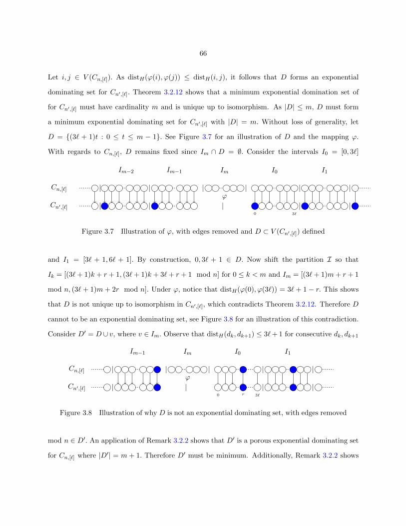
66

Let i, j ∈ V (Cn,[`]). As distH(ϕ(i), ϕ(j)) ≤ distH(i, j), it follows that D forms an exponential

dominating set for Cn′,[`]. Theorem 3.2.12 shows that a minimum exponential domination set of

for Cn′,[`] must have cardinality m and is unique up to isomorphism. As |D| ≤ m, D must form

a minimum exponential dominating set for Cn′,[`] with |D| = m. Without loss of generality, let

D = {(3` + 1)t : 0 ≤ t ≤ m − 1}. See Figure 3.7 for an illustration of D and the mapping ϕ.

With regards to Cn,[`], D remains fixed since Im ∩ D = ∅. Consider the intervals I0 = [0, 3`]

|

Im−2

|

Im−1

|

Im

|

I0

|

I1

|Cn,[`]ϕ

| | |0 3`

| |Cn′,[`]

Figure 3.7 Illustration of ϕ, with edges removed and D ⊂ V (Cn′,[`]) defined

and I1 = [3` + 1, 6` + 1]. By construction, 0, 3` + 1 ∈ D. Now shift the partition I so that

Ik = [(3`+ 1)k + r + 1, (3`+ 1)k + 3`+ r + 1 mod n] for 0 ≤ k < m and Im = [(3`+ 1)m+ r + 1

mod n, (3` + 1)m + 2r mod n]. Under ϕ, notice that distH(ϕ(0), ϕ(3`)) = 3` + 1 − r. This shows

that D is not unique up to isomorphism in Cn′,[`], which contradicts Theorem 3.2.12. Therefore D

cannot to be an exponential dominating set, see Figure 3.8 for an illustration of this contradiction.

Consider D′ = D ∪ v, where v ∈ Im. Observe that distH(dk, dk+1) ≤ 3`+ 1 for consecutive dk, dk+1

|

Im−1

|

Im

|

I0

|

I1

|Cn,[`]ϕ

| |0 r 3`

| |Cn′,[`]

Figure 3.8 Illustration of why D is not an exponential dominating set, with edges removed

mod n ∈ D′. An application of Remark 3.2.2 shows that D′ is a porous exponential dominating set

for Cn,[`] where |D′| = m + 1. Therefore D′ must be minimum. Additionally, Remark 3.2.2 shows

67

that D′ forms a non-porous exponential dominating set. Thus using (3.1.1) we have that⌈n

3`+ 1

⌉≤ γ∗e (Cn,[`]) ≤ γe(Cn,[`]) ≤

⌈n

3`+ 1

⌉.

3.3 Acknowledgements

This research was supported in part by the National Science Foundation Award # 1719841.

We would like to thank Dr. Leslie Hogben for her input on this paper.

3.4 Bibliography



[2] Aysun Aytac and Betul Atay. On exponential domination of some graphs. Nonlinear Dyn.

Syst. Theory, 16(1):12–19, 2016.












68


domination, and porous exponential domination. Discrete Optimization, 23:81–92, 2017.

69

CHAPTER 4. CONCLUDING REMARKS

Overall, exponential domination in graphs is an interesting area within graph theory. The global

influence that exponential dominating vertices exert on the other vertices in the graph is the aspect

about exponential domination that sets it apart from other variants of domination. Notice that

exponential domination is defined with the growth factor of 12 . In the literature, this factor has

remained constant. One avenue for future work would be to explore exponential domination with

a growth factor of p, where 0 < p < 1.

In Chapter 2, a generalized linear programming method was derived to establish lower bounds

for the porous exponential domination number of any graph. In particular for grid graphs, a

technique to improve this lower bound using linear programming was discussed. The difference

between the upper bound constructions and lower bounds derived from this technique for the

porous exponential domination number of the King grid Kn and Slant grid Sn were on the order of

tenths. We believe that additional constraints added to Mixed Integer Linear Program 2.2.3 will

help to further increase the lower bound. In particular see Conjecture 2.5.2, which details the idea

of a global distance α needed to ensure a vertex is dominated, and Conjecture 2.5.7, which suggests

that there exists a minimum porous exponential dominating set with nonadjacent members, for

potential constraints. Notice that the annuli and corresponding partition described in Lemma 2.5.5

and Lemma 2.5.6 did not fully utilize the properties of K∞. For future work, other annuli and

minimal distance between exponential dominating vertices will be examined.

In Chapter 3, it was shown that γ∗e (Cn,[`]) = γe(Cn,[`]) =⌈

n3`+1

⌉. A natural direction would

be to determine bounds or exact values for the porous and non-porous exponential domination

numbers of other types of circulant graphs, and see if the equivalence property of Cn,[`] holds. A

strongly regular graph G, is defined to be a k-regular graph with |V (G)| = n, with the properties

that every two adjacent vertices have λ vertices in common, and every two non-adjacent vertices

70

have µ vertices in common. Observe that Cn,[`] is a strongly regular graph. Another future direction

would be to further study exponential domination on strongly regular graphs. One question would

be to determine whether there is an explicit formula for the porous or non-porous exponential

domination number of a general strongly regular graph. Another interesting question is to find if

there exists a family of strongly regular graphs G for which γe(G) = γ∗e (G).

on exponential domination of graphs michael dairyko

Documents