On Evaluation of Video Quality Metrics:

an HDR Dataset for Computer Graphics Applications

Martin Cadık, Tunc O. Aydın, Karol Myszkowski, Hans-Peter Seidel

MPI Informatik

ABSTRACT

In this paper we propose a new dataset for evaluation of image/video quality metrics with emphasis on applica-tions in computer graphics. The proposed dataset includes LDR-LDR, HDR-HDR, and HDR-LDR reference-testvideo pairs with various types of distortions. We also present an example evaluation of recent image and videoquality metrics that were applied in the field of computer graphics. In this evaluation all video sequences wereshown on an HDR display, and subjects were asked to mark the regions where they saw differences between testand reference videos. As a result, we capture not only the magnitude of distortions, but also their spatial distri-bution. This has two advantages: on one hand the local quality information is valuable for computer graphicsapplications, on the other hand the subjectively obtained distortion maps are easily comparable to the mapspredicted by quality metrics.

1. INTRODUCTION

Experimental evaluation of computer graphics (CG) techniques is necessary to validate their impact on perceivedquality of resulting images. So far such image quality evaluation in CG is mostly performed informally withoutreferring to well-established subjective and objective methods, which are commonly used in other fields, such asin image compression. In particular, CG field could benefit greatly from objective quality metrics due to thesimplicity of their use and low costs involved. This however, requires extensive perceptual validation of suchimage and video quality metrics, which should be sensitive to image artifacts and distortions specific in CG.Another important aspect of such validation is high dynamic range (HDR) of images that are often generated byHDR rendering pipelines, which are today common in computer games (utilizing GPU or specialized consoles)and computer-aided design systems (in particular dealing with realistic image synthesis).

To make the validation (or calibration) of image or video quality metric possible, one needs to design a setof input stimuli (i.e. a dataset) and perform a user study which results in a set of subjective (mean) opinionscores. Subjective studies are very laborious and may be stimuli dependent, thus the community benefits frompublicly available, standardized data sets. Therefore, a few datasets were published in the past.1–5

Unfortunately, none of the existing datasets is suitable for evaluation of video quality metrics in computergraphics field, where the images and videos often exhibit high dynamic range of luminance values and specificartifacts (see Figures 1, 2). Existing datasets are limited in dynamic range of the input stimuli (only low-dynamic (LDR) range videos), in the distortions they cover (mostly compression-related artifacts), and in theextent of subjective responses (usually the numerical rating of the quality of the stimulus). Few authors employeda concept of image distortion maps6–8 in evaluation of image quality metrics, but this has not been done fortemporal distortions in videos so far. To overcome the above limitations, we propose and make publicly available∗

a new dataset for evaluation of image/video quality metrics with emphasis on applications in computer graphics.Several aspects were influential while designing the dataset: (i) in addition to the assessmet of the quality ofLDR videos, the assessment of high-dynamic range videos, as well as comparing HDR videos with LDR videosand vice versa, and (ii) the outcome of the subjective experiment in the form of distortion maps that showquality prediction as a function of spatial position which is especially important for applications in computergraphics. Furthermore, we show an example evaluation of recent image and video quality metrics that were

Further author information: e-mail: {mcadik, tunc, karol, hpseidel}@mpi-inf.mpg.deMax Planck Institut Informatik, Saarbrucken

∗http://www.mpi-inf.mpg.de/resources/hdr/quality

applied in the field of computer graphics. The goal of this evaluation was to examine the correlation betweenthe objective quality predictions computed by the video quality metrics, and the subjective responses obtainedby the experimental procedure. It is known9 that applications of image/video quality metrics into the field ofcomputer graphics are still far from maturity, we believe however, that the published dataset helps in validationand improvement of existing, and the design of future metrics for computer graphics and other applications.

To that end the proposed dataset and the subjective study have the following unique features over previousstudies on video quality assessment:

• The test set includes LDR-LDR, HDR-HDR, and HDR-LDR reference-test video pairs with various typesof distortions.

• A BrightSide DR37-P HDR display (max. luminance ≈ 3000 cd/m2) was used for displaying the videos.

• The subjects were not asked to assess only an overall quality of the video, but to mark the regions wherethey saw differences between test and reference videos, resulting in distortion maps similar to the metricoutcome.

In the remainder of this paper we describe the proposed dataset for evaluation of video quality metrics, theexperimental setup and procedure (Section 2), present an example evaluation of video quality metrics using thedataset (Section 3) and discuss the results based on the correlation between the outcome of the subjective dataand corresponding predictions of state-of-the art video quality metrics.

Figure 1. An example of typical artifacts in rendered images and video sequences: an indoor scene rendered usingprogressive photon mapping algorithm.10 Left: non-converged solution (2 iterations) exhibits low-frequency noise. Right:fully converged solution.

2. DATASET FOR VIDEO METRIC EVALUATION

The proposed dataset consists of 9 reference-test video pairs (1 LDR-LDR, 2 HDR-LDR, and 6 HDR-HDR), theyare listed in Table 1. The video stimuli were generated by imposing temporally varying visual artifacts to HDRscenes (Figure 3), such as HDR video compression artifacts and temporal random noise along with temporalluminance modulation and tone mapping. The magnitudes of the visual artifacts were carefully selected so thatthere were sub-, near- and supra-threshold distortions present in the experimental videos. In sequences #1-#4, and #9 the temporal random noise was generated by filtering a three dimensional array of random valuesbetween −0.5 and 0.5 by a Gaussian with standard deviations 20 (referred as ”high stddev”) and 5 (referredas ”low stddev”) pixels along each dimension. The magnitude of noise was adjusted by multiplying with twoconstants separately, such that the artifacts are barely visible in one setting (referred as ”low magnitude”), andclearly visible in the other (referred as ”high magnitude”). In sequences #5 and #6, the HDR compression13

Figure 2. An example of artifacts due to the tone mapping of HDR images and HDR video sequences. Left: global tonemapping technique by Pattanaik et al.11 preserves overall image contrast, but results in severe loss of details. Right:gradient-based technique of Fattal et al.12 is able to reproduce virtually all the image details, at the cost of an overallcontrast and contrast reversals (i.e. halo artifacts).

was similarly applied at two levels to the HDR scenes, where the luminance was globally modulated over timeby 0.5% of the maximum scene luminance to vary the visibility of image details over time. Videos generatedby applying tone mapping operators11,12 to each input HDR video frame were used in the dynamic rangeindependent comparisons (sequences #7 and #8).

All test videos consist of 60 frames, and should be presented at 24 fps. In order to faithfully reproduce theluminance values on the HDR display, the response function of the display was measured using a Minolta LS-100 luminance meter. The measurements consisted of 17 samples taken from the displayable luminance range.The sample points were then fitted to a 3rd degree polynomial function, from which 100 points were resampledand stored as a lookup table. Finally, the pixel values for the HDR videos were determined by cubic splineinterpolation between nearest two luminance levels. Furthermore, the displayed luminance of the HDR videoswere measured again at various regions, and whenever necessary, the scenes were slightly recalibrated to ensurethat the displayed luminance values match the actual scene luminance.

# Source Ref. DR Test DR Artifact Type of Test Video1 Cars HDR HDR Noise - high magnitude, low stddev2 Lamp HDR HDR Noise - high magnitude, low stddev3 Desk HDR HDR Noise - low magnitude, low stddev4 Tree HDR HDR Noise - high magnitude, high stddev5 Cafe HDR HDR HDR compression - high quality, luminance mod.6 Tower HDR HDR HDR compression - low quality, luminance mod.7 Cafe HDR LDR Luminance modulation, Pattanaik’s tone mapping8 Lamp HDR LDR Luminance modulation, Fattal’s tone mapping9 Lamp LDR LDR Noise - low magnitude, low stddev

Table 1. List of the experimental stimuli. Refer to text for details.

The participants of the experimental study were 16 subjects of age 23 to 50. They all had near-perfector corrected to normal vision, and were naıve for the purposes of the experiment. Each subject evaluated thequality of the whole test set through a graphical user interface displayed on a BrightSide DR37-P HDR display(Figure 4). In the HDR-HDR, and LDR-LDR comparisons, the task was to mark the regions in the test videowhere visible differences were present with respect to the reference video. In the HDR-LDR comparisons onthe other hand, the subjects were asked to assess the contrast loss and amplification. In the instruction phase

Cars Lamp Desk Tree Cafe TowerFigure 3. The video test set is generated from 6 calibrated HDR scenes (tone mapped for presentation purpose14). Thescene luminance was clipped where it exceeded the maximum display luminance. The displayed luminance of the videosresulting from the scenes were between 0.1 and 3000 cd/m2.

before the experiment, the subjects were asked to mark a grid tile even if visible differences were present onlyin a portion of that grid’s area. They were also encouraged to mark a grid tile in the case they cannot decidewhether it contains a visible difference or not. The subjects were placed 0.75 meters away from the display sothat a 512 × 512 image spanned 16 visual degrees and the grid cell size was approximately 1 visual degree. Theenvironment illumination was dimmed and controlled, and all subjects were given time to adapt to the roomillumination. There were no time limitations set for the experiment, but the majority of the subjects took 15-30minutes for the entire test set.

The marked regions for each trial were stored as distortion maps with 16 × 16 resolution, which were thenaveraged over all subjects to find the mean subjective response, see Figure 6 (first column). The descriptivestatistics of these maps are summarized in Table 2 (first column). Figure 5 shows the standard deviation foreach stimulus over the test subjects, separately for each grid tile. Over all images, the minimum and maximumvalues are obtained as 0 and 0.51, the former indicating the tiles on which all subjects gave the same response,and the latter indicating the tiles where approximately half of the subjects have marked.

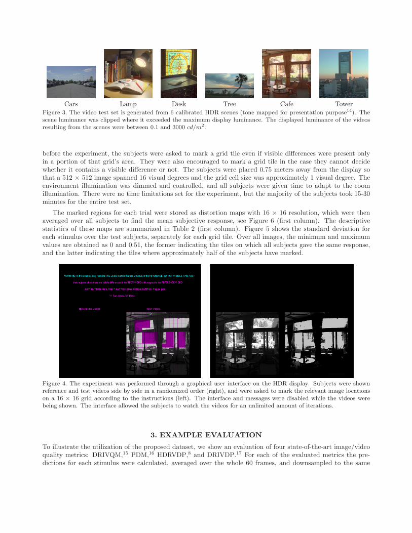
Figure 4. The experiment was performed through a graphical user interface on the HDR display. Subjects were shownreference and test videos side by side in a randomized order (right), and were asked to mark the relevant image locationson a 16 × 16 grid according to the instructions (left). The interface and messages were disabled while the videos werebeing shown. The interface allowed the subjects to watch the videos for an unlimited amount of iterations.

3. EXAMPLE EVALUATION

To illustrate the utilization of the proposed dataset, we show an evaluation of four state-of-the-art image/videoquality metrics: DRIVQM,15 PDM,16 HDRVDP,8 and DRIVDP.17 For each of the evaluated metrics the pre-dictions for each stimulus were calculated, averaged over the whole 60 frames, and downsampled to the same

Stimulus # Subjective Response DRIVQM PDM HDRVDP DRIVDP[min, max]; avg; std [min, max]; avg; std [min, max]; avg; std [min, max]; avg; std [min, max]; avg; std

1 [0.000, 1.000]; 0.177; 0.276 [0.000, 0.850]; 0.128; 0.230 [0.000, 0.301]; 0.082; 0.079 [0.000, 0.019]; 0.001; 0.002 [0.075, 0.417]; 0.194; 0.0582 [0.000, 1.000]; 0.201; 0.347 [0.000, 0.954]; 0.185; 0.282 [0.000, 0.813]; 0.061; 0.138 [0.000, 0.893]; 0.050; 0.157 [0.072, 0.799]; 0.218; 0.1553 [0.000, 1.000]; 0.082; 0.242 [0.000, 0.307]; 0.015; 0.045 [0.000, 0.052]; 0.003; 0.008 [0.000, 0.889]; 0.163; 0.247 [0.006, 0.440]; 0.090; 0.0784 [0.000, 1.000]; 0.124; 0.250 [0.001, 0.457]; 0.094; 0.115 [0.000, 0.024]; 0.007; 0.006 [0.000, 0.000]; 0.000; 0.000 [0.067, 0.240]; 0.137; 0.0395 [0.000, 1.000]; 0.066; 0.186 [0.000, 0.420]; 0.026; 0.063 [0.000, 0.952]; 0.146; 0.207 [0.000, 0.866]; 0.074; 0.166 [0.040, 0.873]; 0.241; 0.1996 [0.000, 1.000]; 0.399; 0.389 [0.072, 0.468]; 0.232; 0.103 [0.810, 0.984]; 0.965; 0.026 [0.180, 0.942]; 0.657; 0.202 [0.626, 0.928]; 0.789; 0.0587 [0.000, 1.000]; 0.312; 0.392 [0.037, 0.984]; 0.451; 0.342 [0.838, 0.984]; 0.980; 0.018 [0.002, 0.953]; 0.448; 0.327 [0.031, 0.953]; 0.374; 0.2888 [0.000, 0.812]; 0.108; 0.180 [0.041, 0.942]; 0.225; 0.146 [0.606, 0.984]; 0.971; 0.043 [0.005, 0.953]; 0.509; 0.274 [0.148, 0.884]; 0.406; 0.1729 [0.000, 1.000]; 0.105; 0.238 [0.000, 0.502]; 0.054; 0.104 [0.000, 0.396]; 0.032; 0.066 [0.000, 0.211]; 0.006; 0.025 [0.067, 0.577]; 0.176; 0.097

Table 2. Descriptive statistics of distortion maps (depicted in Figure 6) for each input stimulus. Abbreaviations used:min=minimal value, max=maximal value, avg=average value, std=standard deviation, of the distortion map averagedover all subjects/metric responses for a particular stimulus (1-9).

0.2 0.4 0.6 0.8 1

Figure 5. Maps showing the standard deviations over subjects for each stimulus. The numbers refer to the first columnof Table 1.

resolution as the mean subjective response. In all the tests in this paper we used a frequency domain implementa-tion of DRIVQM metric, precisely following the reference publication. We found that using this implementationwas still feasible for the frame sizes and durations of the video sequences in our dataset. For larger sequenceswe also implemented an alternative version of the metric, where the frequency domain channel decomposition isreplaced by a Steerable Pyramid based spatial decomposition (described in Appendix A). A web service basedon this implementation is publicly available at http://drivqm.mpi-inf.mpg.de. The HDRVDP and DRIVDPmetrics are designed for image quality evaluation, thus the video stimuli were evaluated for each frame sepa-rately. For each video pair, we computed the 2D correlation between the mean subjective response and themetric prediction (Table 3) and used the results to evaluate the performance of the metrics. The Figure 6 showsthe mean subjective distortion maps along with the corresponding metrics predictions for visual inspection. Thedescriptive statistics of these maps are summarized in Table 2.

For the purposes of generating the maps in Figure 6, in cases of PDM and HDRVDP we simply used thedistortion maps produced by those metrics. In the DRIVDP case however, the output of the metric is threeseparate maps for contrast loss, amplification and reversal. Thus, it is not clear how to produce a singledistortion map for HDR-HDR and LDR-LDR stimuli. After experimenting with various methods for combining

the distortion maps predicted by DRIVDP, we found that the combined map defined as:

P k,l,m

combined = 1 − (1 − P k,l,m

loss ) · (1 − P k,l,m

ampl ), (1)

gives the best correlation with subjective data. Here, P k,l,m

loss|amplrefer to the detection probability of contrast loss

and amplification at scale k, orientation l, and temporal channel m. The resulting map P k,l,m

combined correspondsto the probability of detecting either contrast loss or amplification at a visual channel. Leaving contrast reversalresulted in slightly improved correlations.

3.1 Discussion

As DRIVQM is the only evaluated metric that was designed specifically for the purposes of dynamic range-independent video quality assessment of computer graphics sequences, it is not surprising that it overcomes theother metrics in most cases. Highest correlations were obtained for the #2 HDR-HDR Lamp stimulus with highmagnitude, low standard deviation noise, and the #7 HDR-LDR Cafe stimulus with luminance modulation andPattanaik’s tone mapping (0.883 and 0.879, respectively). For these two cases, the magnitude of the probabilityof detection predicted by the metric, and the average of the binary maps over subjects obtained experimentallyare also very similar. In other cases, either the magnitudes of the mean subjective maps were lower thanthe corresponding detection probability magnitude predictions (such as #4 Tree HDR-HDR stimulus with highmagnitude, high standard deviation noise, and #9 Lamp LDR-LDR stimulus with noise), or a certain region withvisible distortions was missed out (#1 Cars HDR-HDR stimulus with high magnitude, low standard deviationnoise). For the remaining stimuli, a combination of both deviations can be observed in the metric predictionsand subjective responses. The worst prediction of DRIVQM is (#8, 0.733).

HDRVDP, while capable of evaluating the quality of HDR images, lacks any temporal processing and isgeared towards comparing images with the same dynamic range. The DRIVDP addresses the latter limitation,but still suffers from the former. Consequently, DRIVDP’s predictions for the HDR-LDR stimuli (numbers 7and 8) is slightly better than HDRVDP. PDM, on the other hand, is designed for the video stimuli, but lacksthe HDR and dynamic range independent mechanisms of HDRVDP and DRIVDP, producing the least averagecorrelation with the subjective responses. As shown in Table 3, DRIVQM significantly outperforms others inmost cases. The significant difference in average correlations over the entire test set (last row of Table 3) showsthat overall DRIVQMs predictions are clearly more accurate than others. The corresponding distortion mapspredicted by PDM, HDRVDP and DRIVDP are shown in Figure 6 columns 3 - 5 (averaged and downsampledto 16 × 16 after the computation).

While the relation between the correlation values and distortion maps is obvious in most cases, the highcorrelation of PDM for stimulus #3 deserves further explanation. While PDM correctly detects the distortedregions in that stimulus in a spatial sense, the magnitude of detection probabilities are very low (refer to Table 2),to the point that they are quantized by the visualization. Thus the map appears to be blank, but since the relationwith the subjective data is linear, the correlation is high.

4. CONCLUSION

The main goal of this work was to develop a dataset of video sequences accompanied by the correspondingsubjective data evaluating their quality in a local manner. Such locality is the key in computer graphics applica-tions, where local image distortions should be detected and if possible corrected in rendering. Another importantaspect of such dataset is dynamic range of frames, where pairs of HDR, LDR and mixed LDR-HDR reference andtest videos, which are calibrated in terms of pixel luminance, are considered. We propose also a novel subjectivetesting setup that involves an HDR display, which is suitable for reproducing luminance levels in the videos, aswell as interactive marking of local image regions where distortions are visible.

The dataset proved to be useful in calibrating and validating the DRIVQM,15 which has been developedspecifically for computer graphics applications. The dataset is publicly available (http://www.mpi-inf.mpg.de/resources/hdr/quality) and our hope is that it can be used in other validation tasks.

Stimulus # DRIVQM PDM HDRVDP DRIVDP1 0.765 -0.0147 0.591 0.4882 0.883 0.686 0.673 0.8593 0.843 0.886 0.0769 0.8654 0.815 0.0205 0.211 -0.06545 0.844 0.565 0.803 0.6896 0.761 -0.462 0.709 0.2997 0.879 0.155 0.882 0.9248 0.733 0.109 0.339 0.3939 0.753 0.368 0.473 0.617

Average 0.809 0.257 0.528 0.563

Table 3. Correlations of subjective responses with predictions of DRIVQM, PDM, HDRVDP, and DRIVDP. The last rowshows the average correlations over the test set, the best correlations for each stimulus are printed in bold text.

APPENDIX A. EFFICIENT IMPLEMENATATION OF DRIVQM

As we admit in the discussion section of the previous publication,15 executing DRIVQM becomes infeasible forlong video sequences due to the long processing time. Moreover, the 64-frames window size practically meansthat for frame sizes larger than VGA the memory consumption is prohibitively large for an average desktopcomputer. As suggested by the authors of the metric, we replace the frequency domain Cortex Transform bythe Steerable Pyramid18 with 6 levels (where each differ by one octave) and 6 orientations, and use Winkler’s19

9-tap approximation of the transient and sustained temporal mechanisms. The base band of the SteerablePyramid, analogous to Cortex Transform, does not have any orientations. For the purpose of accounting forspatial phase uncertainty, the Hilbert transforms of the steerable filters provided by Freeman and Adelson’sformulation are used, whereas temporal phase uncertainty is ignored. All other components of the DRIVQMare left intact, including the extended Contrast Sensitivity Function. The updated implementation is moreefficient in memory consumption and running time, without any significant deviation in results from the originalimplementation. A publicly available web service that uses our updated implementation can be found at http://drivqm.mpi-inf.mpg.de. The web service requires the users to upload the frames of their test and referencevideo pair of either the same dynamic range, or different dynamic ranges. Users are allowed to change metricparameters, such as the pixels per visual degree, frames per second and adaptation luminance. Once the setupis complete, the metric is run on the uploaded video pair. Upon completion, the input video pair is immediatelydeleted, and the user is provided with a link to the contrast difference, contrast loss, and contrast amplificationmaps.

ACKNOWLEDGMENTS

The authors would like to thank all the staff members and students at MPI Informatik who kindly participatedin the subjective experiments.

REFERENCES

[1] Carney, T., Klein, S. A., Tyler, C. W., Silverstein, A. D., Beutter, B., Levi, D., Watson, A. B., Reeves, A. J.,Norcia, A. M., Chen, C.-C., Makous, W., and Eckstein, M. P., “The development of an image/thresholddatabase for designing and testing human vision models,” in [Proc. of Human Vision, Visual Processing,and Digital Display IX ], SPIE, Bellingham, WA, 3644 (1999).

[2] The Video Quality Experts Group, “Final report from the video quality experts group on the validationof objective quality metrics for video quality assessment, Phase I.” http://www.its.bldrdoc.gov/vqeg/

projects/frtv (2000).

[3] Sheikh, H. R. and Bovik, A. C., “LIVE image quality assessment database.” http://live.ece.utexas.

edu/research/quality/subjective.htm (2003).

[4] Seshadrinathan, K., Soundararajan, R., Bovik, A. C., and Cormack, L. K., “LIVE video quality database.”http://live.ece.utexas.edu/research/quality/live_video.html (November 2009).

[5] Seshadrinathan, K., Soundararajan, R., Bovik, A. C., and Cormack, L. K., “A subjective study to evaluatevideo quality assessment algorithms,” Human Vision and Electronic Imaging XV 7527(1), 75270H, SPIE(2010).

[6] Zhang, X., Setiawan, E., and Wandell, B., “Image distortion maps,” in [Fifth Color Imaging Conference:Color Science, Systems and Applications ], 120–125 (1997).

[7] Zhang, X. and Wandell, B. A., “Color image fidelity metrics evaluated using image distortion maps,” SignalProcessing 70(3), 201 – 214 (1998).

[8] Mantiuk, R., Daly, S., Myszkowski, K., and Seidel, H.-P., “Predicting visible differences in high dynamicrange images - model and its calibration,” in [Human Vision and Electronic Imaging X ], SPIE ProceedingsSeries 5666, 204–214 (2005).

[9] Rogowitz, B. E. and Rushmeier, H. E., “Are image quality metrics adequate to evaluate the quality ofgeometric objects?,” in [Proc. of Human Vision and Electronic Imaging VI ], 340–348, SPIE (2001).

[10] Hachisuka, T., Ogaki, S., and Jensen, H. W., “Progressive photon mapping,” in [ACM Transactions onGraphics (Proc. of SIGGRAPH Asia’08) ], 27(5), 1–8, ACM, New York, NY, USA (2008).

[11] Pattanaik, S. N., Tumblin, J. E., Yee, H., and Greenberg, D. P., “Time-dependent visual adaptation forfast realistic image display,” in [ACM Transactions on Graphics (Proc. of ACM SIGGRAPH’00) ], 47–54,ACM Press (2000).

[12] Fattal, R., Lischinski, D., and Werman, M., “Gradient domain high dynamic range compression,” in [ACMTransactions on Graphics (Proc. of ACM SIGGRAPH’02) ], 249–256, ACM Press (2002).

[13] Mantiuk, R., Krawczyk, G., Myszkowski, K., and Seidel, H.-P., “Perception-motivated high dynamic rangevideo encoding,” in [ACM Transactions on Graphics (Proc. of SIGGRAPH’04) ], 23(3), 733–741, ACM(2004).

[14] Reinhard, E., Stark, M., Shirley, P., and Ferwerda, J., “Photographic tone reproduction for digital images,”in [ACM Transactions on Graphics (Proc. of SIGGRAPH’02) ], 267–276, ACM Press (2002).

[15] Aydın, T. O., Cadık, M., Myszkowski, K., and Seidel, H.-P., “Video quality assessment for computergraphics applications,” in [ACM Transactions on Graphics (Proc. of SIGGRAPH Asia’10) ], 1–10, ACM,Seoul, Korea (2010).

[16] Winkler, S., [Digital Video Quality: Vision Models and Metrics ], Wiley (2005).

[17] Aydın, T. O., Mantiuk, R., Myszkowski, K., and Seidel, H.-P., “Dynamic range independent image qualityassessment,” in [ACM Transactions on Graphics (Proc. of ACM SIGGRAPH’08) ], 27(3) (2008). Article69.

[18] Freeman, W. T. and Adelson, E. H., “The design and use of steerable filters,” Pattern Analysis and MachineIntelligence, IEEE Transactions on 13(9), 891–906 (1991).

[19] Winkler, S., “A perceptual distortion metric for digital color video,” in [Proc. of Human Vision and Elec-tronic Imaging, SPIE ], Controlling Chaos and Bifurcations in Engineering Systems 3644, 175–184, IEEE(1999).

Subj. Response DRIVQM PDM HDRVDP DRIVDP

#1

#2

#3

#4

#5

Subj. Response DRIVQM PDM HDRVDP DRIVDP

#6

#7

#8

#9

0.2 0.4 0.6 0.8 1

Figure 6. Mean subjective response distortion maps and corresponding mean metric predictions pairs.