1

On DSGE Models*

Lawrence J. Christiano† Martin S. Eichenbaum‡ Mathias Trabandt§

April 26, 2018

*Prepared for the Journal of Economic Perspectives. We are grateful for the comments of Olivier Blanchard, Robert Gordon, Narayana Kocherlakota, Douglas Laxton, Edward Nelson, Giorgio Primiceri and Sergio Rebelo on an earlier draft of this paper.

†Northwestern University, Department of Economics, 2211 Campus Drive, Evanston, Illinois 60208, USA.

Phone: +1-847-491-8231. E-mail: l-christiano@northwestern.edu. ‡Northwestern University, Department of Economics, 2211 Campus Drive, Evanston, Illinois 60208, USA.

Phone: +1-847-491-8232. E-mail: eich@northwestern.edu. §Freie Universitat Berlin, School of Business and Economics, Chair of Macroeconomics,

Boltzmannstrasse 20, 14195 Berlin, Germany and Halle Institute for Economic Research (IWH), E-mail: mathias.trabandt@gmail.com.

2

1 Introduction

The outcome of any important macroeconomic policy change is the net effect of forces

operating on different parts of the economy. A central challenge facing policy makers is how

to assess the relative strength of those forces. Economists have a range of tools that can be

used to make such assessments. Dynamic stochastic general equilibrium (DSGE) models are

the leading tool for making such assessments in an open and transparent manner.

To be concrete, suppose we are interested in understanding the effects of a systematic

change in policy, like switching from inflation targeting to price-level targeting. The most

compelling strategy would be to do randomized control trials on actual economies. But, that

course of action is not available to us. So, what are the alternatives? It is certainly useful to

study historical episodes in which such a similar policy switch occurred or to use reduced-

form time series methods. But, there are obvious limitations to each of these approaches. In

the historical approach, the fact that no two episodes are exactly the same always raises

questions about the relevance of a past episode for the current situation. In the case of

reduced-form methods, it is not always clear which parameters should be changed and

which should be kept constant across policy options. Inevitably, assessing the effects of a

systematic policy change has to involve the use of a model.

To be useful for policy analysis, DSGE models must be data based. As a practical matter,

macroeconomic data aren’t sufficient for discriminating between many alternative models

that offer different answers to policy questions. Put differently, many DSGE models are

observationally equivalent with respect to macro data. But modern DSGE models are based

on microeconomic foundations. So, microeconomic data and institutional facts can be

brought to bear on the design, construction and evaluation of DSGE models. Micro data

break the observational equivalence that was the bane of macroeconomists.

The openness and transparency of DSGE models is a virtue. But it also makes them easy to

criticize. Suspicious assumptions can be highlighted. Inconsistencies with the evidence can

easily be spotted. Forces that are missing from the model can be identified. The process of

responding to informed criticisms is a critical part of the process of building better DSGE

models. Indeed, the transparent nature of DSGE models is exactly what makes it possible for

diverse groups of researchers - including those who don’t work on DSGE models - to be part

of the DSGE project.

Some analysts object to working with DSGE models and prefer to instead think about policy

by working with small equilibrium models that emphasize different subsets of the economy,

labor or financial markets. This approach has a vital contribution to make because small

models help us build intuition about the mechanisms at work in DSGE models. But, this

approach cannot be a substitute for DSGE models itself because quantitative conclusions

about the overall economic impact of a policy requires informal judgment as one integrates

across individual small-scale models. The small-model approach to policy thus involves

3

implicit assumptions and lacks the transparency of the DSGE approach.

To be clear, policy decisions are made by real people using their best judgment. Used wisely,

DSGE models can improve and sharpen that judgment. In an ideal world, we will have both

wise policymakers and empirically plausible models. But, to paraphrase Fischer (2017)’s

paraphrase of Samuelson on Solow: “We’d rather have Stanley Fischer than a DSGE model,

but we’d rather have Stanley Fischer with a DSGE model than without one.”

In section 2 we review the state of mainstream DSGE models before the financial crisis and

the Great Recession. In section 3 we describe how DSGE models are estimated and

evaluated. Section 4 addresses the question of why DSGE modelers – like most other

economists and policy makers – failed to predict the financial crisis and the Great Recession.

Section 5 discusses how DSGE modelers responded to the financial crisis and its aftermath.

Section 6 discusses how current DSGE models are actually used by policy makers. Section 7

provides a brief response to criticism of DSGE models, with special emphasis on Stiglitz

(2017). Section 7 offers concluding remarks.

2 Before the Storm

In this section we describe early DSGE models and how they evolved prior to the crisis.

2.1 Early DSGE Models

As a practical matter, people often use the term DSGE models to refer to quantitative

models of growth or business cycle fluctuations. A classic example of a quantitative DSGE

model is the Real Business Cycle (RBC) model associated with Kydland and Prescott (1982)

and Long and Plosser (1983). These early RBC models imagined an economy populated by

households who participate in perfectly competitive goods, factor and asset markets. These

models took the position that fluctuations in aggregate economic activity are an efficient

response of the economy to the one source of uncertainty in agents’ environment,

exogenous technology shocks. The associated policy implications are clear: there is no need

for any form of government intervention. In fact, government policies aimed at stabilizing

the business cycle are welfare-reducing.

Excitement about RBC models crumbled under the impact of three forces. First, micro data

cast doubt on some of the key assumptions of the model. These assumptions include, for

example, perfect credit and insurance markets, as well as perfectly frictionless labor markets

in which fluctuations in hours worked reflect movements along a given labor supply curve or

optimal movements of agents in and out of the labor force (see Chetty et al. (2011)). Second,

the models had difficulty in accounting for some key properties of the aggregate data, such

as the observed volatility in hours worked, the equity premium, the low co-movement

of real wages and hours worked (see Christiano and Eichenbaum (1992) and King and

Rebelo (1999)). Open-economy versions of these models also failed to account for key

4

observations such as the cyclical co-movement of consumption and output across

countries (see Backus et al. (1992)) and the extremely high correlation between nominal

and real exchange rates (see Mussa (1986)).

Third, because money plays no role in RBC models, those models seem inconsistent with

mainstream interpretations of various historical episodes. One example is Hume (1742)’s

description of how money from the New World affected the European economy. A different

example is the view that the earlier a country abandoned the Gold Standard during the Great

Depression, the sooner its recovery began (see Bernanke (1995)). A final example is the view

that RBC models don’t shed light on the severe recession associated with the Volcker

disinflation.

Finally, the simple RBC model is effectively mute on a host of policy-related issues that are of

vital importance to macroeconomists and policy makers. Examples include: what are the

consequences of different monetary policy rules for aggregate economic activity, what are

the effects of alternative exchange rate regimes, and what regulations should we impose on

the financial sector?

2.2 New Keynesian Models

Prototypical pre-crisis DSGE models built upon the chassis of the RBC model to allow for

nominal frictions, both in labor and goods markets. These models are often referred to as

New Keynesian DSGE models. But, it would be just as appropriate to refer to them as

Friedmanite DSGE models. The reason is that they embody the fundamental world view

articulated in Friedman’s seminal Presidential Address (see Friedman (1968)). According to

this view, hyperinflations aside, monetary policy has essentially no impact on real variables

like output and the real interest rate in the long run. However, due to sticky prices and wages

monetary policy matters in the short run.1 Specifically, a policy-induced transitory fall in the

nominal interest rate is associated with a decline in the real interest rate, an expansion in

economic activity and a moderate rise in inflation.

Models in which permanent changes in monetary policy induce roughly one-to-one changes

in inflation and the nominal rate of interest are said to satisfy the Fisherian property. Models

in which transitory changes in monetary policy induce movements in nominal interest rates

and inflation of the opposite sign are said to satisfy the anti-Fisherian property. The canonical

New Keynesian models of Yun (1996) and Clarida et al. (1999) and Woodford (2003) satisfy

both properties.

1 For example, Friedman (1968, p. 10) writes that after the monetary authority increases money growth,

“... much or most of the rise in income will take the form of an increase in output and employment

rather than in prices. People have been expecting prices to be stable, and prices and wages have been set

for some time in the future on that basis. It takes time for people to adjust to a new state of

demand. Producers will tend to react to the initial expansion in aggregate demand by increasing output,

employees by working longer hours, and the unemployed, by taking jobs now offered at former nominal

wages.”

5

The basic intuition behind the anti-Fisherian property of the New Keynesian model is as

follows. Firms set their prices on the basis of current and future marginal costs. The future

state of the economy is relatively unaffected by a transitory monetary policy shock. So, actual

inflation responds relatively little to a policy induced transitory fall in the nominal interest

rate. As a result, the real interest rate declines. Intertemporal substitution by households

then induces a rise in current consumption, leading to a rise in labor income. That increase

reinforces the contemporaneous rise in consumption and employment. The expansion in

employment drives wages and marginal costs up. The latter effect drives inflation up. Since

inflation and the nominal interest move in opposite directions, the model has the anti-

Fisherian property. Less surprisingly, standard New Keynesian models satisfy the Fisherian

property because its long-run properties are roughly the same as the underlying RBC chassis.

Many researchers found New Keynesian models attractive because they seemed sensible

and they allowed researchers to engage in the types of policy debates that RBC models had

been silent about. A critical question was: what properties should quantitative versions of

these models have? To address this question, the empirical literature focused on quantifying

the dynamic effects of a shock to monetary policy. This type of shock has long been of

interest to macroeconomists for a variety of reasons. For example, Friedman and Schwartz

(1963) attributed the major portion of business cycle variations to exogenous shocks in the

money supply. The recent literature finds these shocks interesting because they provide a

potentially powerful diagnostic for discriminating between models. Perhaps the most

extreme example is that a real business cycle model implies nothing happens to real

variables after a monetary policy shock. Simple New Keynesian models imply that real

variables do respond to a monetary policy shock.

A monetary policy shock can reflect a variety of factors including measurement error in the

real-time data that policy makers condition their actions on and the basic randomness that is

inherent in group decisions. In a seminal paper Sims (1986) argued that one should identify

monetary policy shocks with disturbances to a monetary policy reaction function in which

the policy instrument is a short-term interest rate. Bernanke and Blinder (1992) and

Christiano et al. (1996, 1999) identify monetary policy shocks using the assumption that

monetary policy shocks have no contemporaneous impact on inflation and output.2 This set

of identifying restrictions, like the entire New Keynesian enterprise, falls squarely in the

Friedman world view. For example, in testimony before Congress, Friedman (1959) said:

“Monetary and fiscal policy is rather like a water tap that you turn on now and that then only starts to run 6, 9, 12, 16 months from now.”

In practice, this Friedman-style identifying strategy is implemented using a vector

autoregression representation (VAR) with a large set of variables. Figure 1 displays the

effects of identified monetary policy shocks estimated using data covering the period

1951Q1 to 2008Q4. For convenience we only show the response functions for a subset of the

2 Christiano, Eichenbaum and Evans (1999) show that the results from imposing this assumption on monthly or quarterly data are qualitatively similar. The assumption is obviously more compelling for monthly data.

6

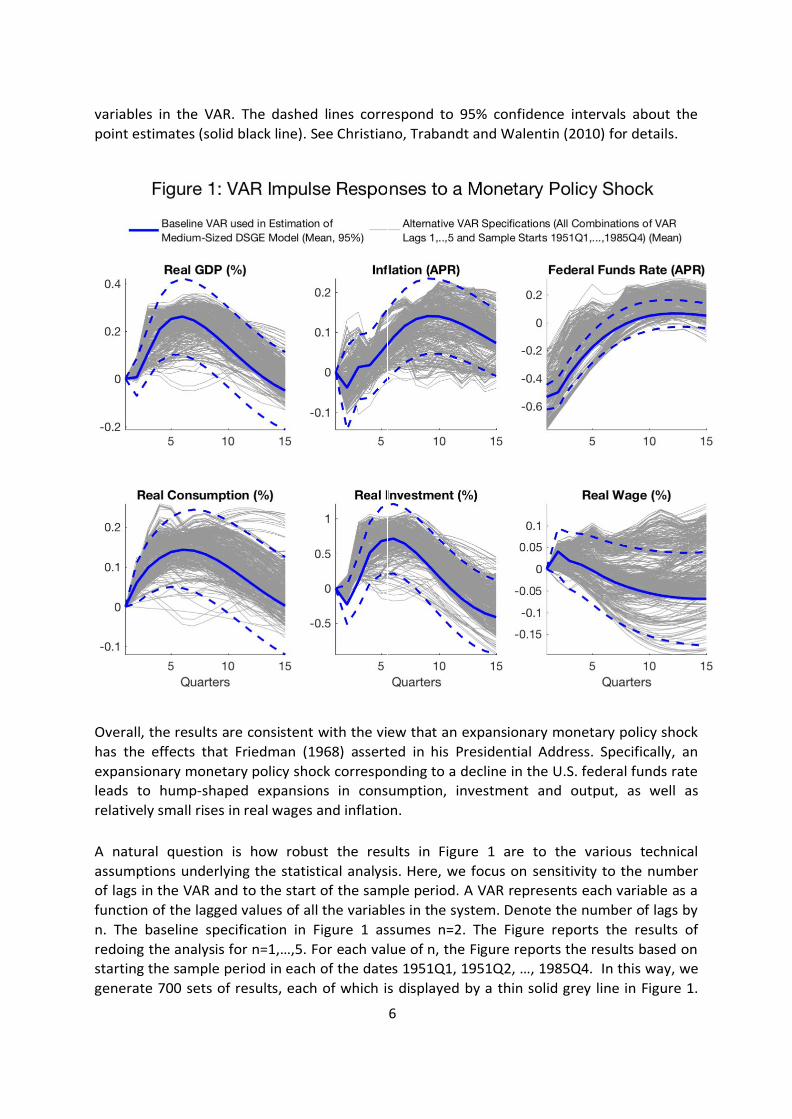
variables in the VAR. The dashed lines correspond to 95% confidence intervals about the

point estimates (solid black line). See Christiano, Trabandt and Walentin (2010) for details.

Overall, the results are consistent with the view that an expansionary monetary policy shock

has the effects that Friedman (1968) asserted in his Presidential Address. Specifically, an

expansionary monetary policy shock corresponding to a decline in the U.S. federal funds rate

leads to hump-shaped expansions in consumption, investment and output, as well as

relatively small rises in real wages and inflation.

A natural question is how robust the results in Figure 1 are to the various technical

assumptions underlying the statistical analysis. Here, we focus on sensitivity to the number

of lags in the VAR and to the start of the sample period. A VAR represents each variable as a

function of the lagged values of all the variables in the system. Denote the number of lags by

n. The baseline specification in Figure 1 assumes n=2. The Figure reports the results of

redoing the analysis for n=1,…,5. For each value of n, the Figure reports the results based on

starting the sample period in each of the dates 1951Q1, 1951Q2, …, 1985Q4. In this way, we

generate 700 sets of results, each of which is displayed by a thin solid grey line in Figure 1.

7

Note that the basic qualitative properties of the benchmark analysis are remarkably robust,

although there are of course specifications of n and the sample period that yield different

implications. It is interesting how similar the shape of the confidence and sensitivity intervals

are.

In recent years researchers have developed alternative procedures for identifying monetary

policy shocks. These procedures focus on movements in the federal funds futures rate in a

tight window of time around announcements made by monetary policy makers. See, for

example, Gertler and Karadi (2015) who build on the work of Kuttner (2001) and Gürkaynak,

Sack and Swanson (2005). Broadly speaking, this literature reaches the same conclusions

about the effects of monetary policy shocks displayed in Figure 1. In our view, these

conclusions summarize the conventional view about the effects of a monetary policy shock.

2.3 Christiano, Eichenbaum and Evans’ Model

A key challenge was to develop an empirically plausible version of the New Keynesian

model that could account quantitatively for the type of impulse response functions

displayed in Figure 1. Christiano et al. (2005) developed a version of the New Keynesian

model that met this challenge. We go into some detail describing the basic features of

that model because they form the core of leading pre-crisis DSGE models, such as Smets

and Wouters (2003, 2007).

2.3.1 Consumption and Investment Decisions

Consistent with a long tradition in macroeconomics, the model economy in Christiano et al.

(2005) is populated by a representative household. At each date, the household allocates

money to purchases of financial assets, as well as consumption and investment goods. The

household receives income from wages, from renting capital to firms and from financial

assets, all net of taxes.

As in the simple New Keynesian model, Christiano et al. (2005) make assumptions that imply

the household’s borrowing constraints are not binding. So, the interest rate determines the

intertemporal time pattern of consumption. Of course, the present value of income

determines the level of consumption. Holding interest rates constant, the solution to the

household problem is consistent with a key prediction of Friedman’s permanent income

hypothesis: persistent changes in income have a much bigger impact on household

consumption than transitory changes.

To be consistent with the response of consumption and the interest rate to a monetary

policy shock observed in Figure 1, Christiano et al. (2005) had to depart from the standard

assumption that utility is time-separable in consumption. Generally speaking, that

assumption implies households choose a declining path for consumption in response to a

low interest rate. The household’s intertemporal budget constraint then implies that after a

policy-induced decline in the interest rate, consumption jumps immediately and then falls.

8

But, this is a very different pattern than the hump-shape response that we see in Figure 1.

To remedy this problem, Christiano et al. (2005) follow Fuhrer (2000) by adopting the

assumption of habit-formation in consumption. Under this specification, the marginal utility

of current consumption depends positively on the level of the household’s past

consumption. Households then choose to raise consumption slowly over time, generating a

hump-shape response-pattern as in Figure 1. As it turns out, there is substantial support for

habit persistence in the finance, growth and psychology literatures.3

To be consistent with the hump-shape response of investment to a monetary policy shock,

Christiano et al. (2005) had to assume households face costs of changing the rate of

investment. To see why, note that absent uncertainty, arbitrage implies that the one-period

return on capital is equal to the real rate of interest on bonds. Absent any adjustment costs,

the one-period return on capital is the sum of the marginal product of capital plus one

minus the depreciation rate. Suppose that there is an expansionary monetary policy shock

that drives down the real interest rate, with the maximal impact occurring

contemporaneously, as in the data (see Figure 1). Arbitrage requires that the one period

return on capital and the marginal product of capital follow a pattern identical to the real

interest rate. For that to happen both the capital stock and investment must have exactly

the opposite pattern than the marginal product of capital. With the biggest surge in

investment occurring in the period of the monetary policy shock the simple model cannot

reproduce the hump-shape pattern in Figure 1. When it is costly to adjust the rate of

investment, households choose to raise investment slowly over time, generating a hump-

shape response-pattern as in Figure 1.

Lucca (2006) and Matsuyama (1984) provide interesting theoretical foundations for the

investment adjustment cost in Christiano et al. (2005). In addition, there is substantial

empirical evidence in support of the specification (see Eberly et al. (2012) and Matsuyama

(1984)).

An important alternative specification of adjustment costs penalizes changes in the capital

stock. This specification has a long history in macroeconomics, going back at least to Lucas

and Prescott (1971). Christiano, Eichenbaum and Evans show that with this type of

adjustment cost, investment jumps after an expansionary monetary policy shock and then

converges monotonically back to its pre-shock level from above. This response pattern is

inconsistent with the VAR evidence.

2.3.2 Nominal Rigidities

In contrast to RBC models, goods and labor markets in Christiano et al. (2005) are not

perfectly competitive. This departure is necessary to allow for sticky prices and sticky

3 In the finance literature see, for example, Eichenbaum and Hansen (1990), Constantinides (1990) and

Boldrin et al. (2001). In the growth literature see Carroll et al. (1997, 2000). In the psychology literature, see

Gremel et al. (2016).

9

nominal wages – if a price or wage is sticky, someone has to set it.

In Christiano et al. (2005), nominal rigidities arise from Calvo (1983) style frictions. In

particular, firms and households can change prices or wages with some exogenous

probability. In addition, they must satisfy whatever demand materializes at those prices and

wages.

Calvo-style frictions make sense only in environments where inflation is moderate. Even in

moderate inflation environments, Calvo-style frictions have implications that are

inconsistent with aspects of micro data (see for example Nakamura and Steinsson (2008) or

Eichenbaum et al. (2011)). Still, its continued use reflects the fact that Calvo-style frictions

allow models to capture, in an elegant and tractable manner, what many researchers

believe is an essential feature of business cycles. In particular, for moderate inflation

economies, firms and labor suppliers typically respond to variations in demand by varying

quantities rather than prices.

2.3.3 A-cyclical Marginal Costs

Christiano et al. (2005) build features into the model which ensure that firms’ marginal costs

are nearly a-cyclical. They do so for three reasons. First, there is substantial empirical

evidence in favor of this view (see for example, Anderson et al. (2018)). Second, the more a-

cyclical marginal cost is, the more plausible is the assumption that firms satisfy demand.

Third, as in standard New Keynesian models, inflation is an increasing function of current

and expected future marginal costs. So, relatively a-cyclical marginal costs are critical for

dampening movements in the inflation rate.

The model in Christiano et al. (2005) incorporates two mechanisms to ensure that marginal

costs are relatively a-cyclical. The first is the sticky nominal wage assumption mentioned

above. The second mechanism is that the rate at which capital is utilized can be varied in

response to shocks.

2.3.4 Quantitative Properties To illustrate the model’s quantitative properties, we work with the variant of the model of

Christiano et al. (2005) estimated by Christiano, Eichenbaum and Trabandt (2016). We re-

estimated the model using a Bayesian procedure that treats the VAR-based impulse

responses to a monetary policy shock as data. The appendix to this paper provides details

about the prior and posterior distributions of model parameters. Here we highlight some of

the key estimated parameters. The posterior mode estimates imply that firms change prices

on average once every 2.3 quarters, the household changes nominal wages about once a

year, past consumption enters with a coefficient of 0.75 in the household’s utility function,

and the elasticity of investment with respect to a one percent temporary increase in the current

price of installed capital is equal to 0.16.

10

The solid black lines in Figure 2 are the VAR-based impulse response function estimates

reproduced from Figure 1. The grey area depicts the 95% confidence intervals associated

with those estimates. The solid blue line depicts the impulse response function of the DSGE

model to a monetary policy shock, calculated using the mode of the posterior distribution of

the model’s parameters.

Four key features of the results are worth noting. First, the model succeeds in accounting

for the hump-shape rise in consumption, investment and real GDP after a policy-induced fall

in the federal funds rate. Second, the model succeeds in accounting for the small rise in

inflation after the shock. Third, the model has the property that real wages are essentially

unaffected by the policy shock. Finally, the model has the anti-Fisherian property that the

nominal interest and inflation move in the opposite direction after a transitory monetary

policy shock.

We emphasize that the model’s properties depend critically on sticky wages. The red

dashed line in Figure 2 depicts the model’s implications if we recalculate the impulse

responses assuming that nominal wages are fully flexible (holding other model parameters

fixed at the mode of the posterior distribution). Note that the model’s performance

11

deteriorates drastically. Of course sticky wages are not the only way to mute the sensitivity

of real wages to a monetary policy shock. See CET (2016) for an exploration and discussion

of alternatives, including search and matching labor market models that have rich

implications for unemployment and labor force participation rates. The key point is that any

successful DSGE model must have the property that real wages and marginal costs are

essentially a-cyclical.

Finally, we note that habit formation and investment adjustment costs are critical to the

model’s success. Absent those features, it would be very difficult to generate hump-shaped

responses with reasonable degrees of nominal rigidities.

3 How DSGE Models Are Estimated and Evaluated

Prior to the financial crisis, researchers generally worked with log-linear approximations to

the equilibria of DSGE models. There were three reasons for this choice. First, for the

models being considered and for the size of shocks that seemed relevant for the post-war

U.S. data, linear approximations are very accurate (see for example the papers in Taylor and

Uhlig (1990)). Second, linear approximations allow researchers to exploit the large array of

tools for forecasting, filtering and estimation provided in the literature on linear time series

analysis. Third, it was simply not computationally feasible to solve and estimate large,

nonlinear DSGE models. The technological constraints were real and binding.

Researchers choose values for the key parameters of their models using a variety of

strategies. In some cases, researchers choose parameter values to match unconditional

model and data moments, or they reference findings in the empirical micro literature. This

procedure is called calibration and does not use formal sampling theory. Calibration was

the default procedure in the early RBC literature and it is also sometimes used in the DSGE

literature. Most of the modern DSGE literature conducts inference about parameter values

and model fit using one of two strategies that make use of formal econometric sampling

theory.

The first strategy is limited information because it does not exploit all of the model’s

implications for moments of the data. One variant of the strategy minimizes the distance

between a subset of model-implied second moments and their analogs in the data. A more

influential variant of this first strategy estimates parameters by minimizing the distance be-

tween model and data impulse responses to economic shocks (examples of the impulse

response matching approach include Christiano et al. (2005), Altig et al. (2011), Iacoviello

(2005) and Rotemberg and Woodford (1991)).

One way to estimate the data impulse response functions is based on partially identified

VARs. Another variant of this strategy, sometimes referred to as the method of external

instruments, involves using historical or narrative methods to obtain instruments for the

underlying shocks (see, Mertens and Ravn (2013)). Finally, researchers have exploited

movements in asset prices immediately after central bank policy announcements to identify

12

monetary policy shocks and their consequences. This approach is referred to as high

frequency identification (early contributions include e.g. Kuttner (2001) and Gürkaynak et al.

(2005)).

The initial limited information applications in the DSGE literature used generalized method

of moments estimators and classical sampling theory (see Hansen (1982)). Building on the

work of Chernozhukov and Hong (2003), Christiano et al. (2010) showed how the Bayesian

approach can be applied in limited information contexts.

A critical advantage of the Bayesian approach is that one can formally and transparently

bring to bear information from a variety of sources on what constitutes “reasonable” values

for model parameters. Suppose, for example, that one could only match the dynamic

response to a monetary policy shock for model parameter values implying that firms change

their prices on average every two years. This implication is strongly at variance with

evidence from micro data. In the Bayesian approach, the analyst would impose priors that

sharply penalize such parameter values. So, those parameter values would be assigned low

probabilities in the analyst’s posterior distribution. Best practice compares priors and

posteriors for model parameters. This comparison allows the analyst to make clear the role

of priors and the data in generating the results.

As we just stressed the Bayesian approach allows one to bring to bear information culled

from micro data on model parameters. This approach allows one to bring to bear

information culled from micro data on model parameters. At a deeper level, micro data

influences, in a critical but slow-moving manner, the class of models that we work with. Our

discussion of the demise of the pure RBC model is one illustration of this process. The

models of financial frictions and heterogeneous agents discussed below are an additional

illustration of how DSGE models evolve over time in response to micro data (see sections

5.1 and 5.3).

The second strategy for estimating DSGE models involves full-information methods. In many

applications, the data used for estimation is relatively uninformative about the value of

some of the parameters in DSGE models (see Canova and Sala (2009)). A natural way to deal

with this fact is to bring other information to bear on the analysis. Bayesian priors are a

vehicle for doing exactly that. This is an important reason why the Bayesian approach has

been very influential in full-information applications. Starting from Smets and Wouters

(2003), a large econometric literature has expanded the Bayesian toolkit to include better

ways to conduct inference about model parameters and to analyze model fit. For a recent

survey see Fernandez-Villaverde et al. (2016).

4 Why Didn’t DSGE Models Predict the Financial

Crisis?

Pre-crisis DSGE models didn’t predict the increasing vulnerability of the U.S. economy to a

financial crisis. They have also been criticized for not placing more emphasis on financial

13

frictions. Here, we give our perspective on these failures.

There is still an ongoing debate about the causes of the financial crisis. Our view, shared by

Bernanke (2009) and many others, is that the financial crisis was precipitated by a rollover

crisis in a very large and highly levered shadow-banking sector that relied on short-term

debt to fund long-term assets. By shadow banks we mean financial institutions not covered

by the protective umbrella of the Federal Reserve and Federal Deposit Insurance

Corporation (for further discussion, see Bernanke (2010)).

Rollover crisis was triggered by a set of developments in the housing sector. U.S. housing

prices began to rise rapidly in the 1990’s. The S&P/Case-Shiller U.S. National Home Price

Index rose by a factor of roughly 2.5 between 1991 and 2006. The precise role played by

expectations, the subprime market, declining lending standards in mortgage markets, and

overly-loose monetary policy is not critical for our purposes. What is critical is that housing

prices began to decline in mid-2006, causing a fall in the value of the assets of shadow banks

that had heavily invested in mortgage-backed securities. The Fed’s willingness to provide a

safety net for the shadow banking system was at best implicit, creating the conditions under

which a roll-over crisis was possible. In fact, a rollover crisis did occur and shadow banks had

to sell their asset-backed securities at fire-sale prices, precipitating the financial crisis and

the Great Recession.

Against this background, we turn to the first of the two criticisms of DSGE models

mentioned above, namely their failure to signal the increasing vulnerability of the U.S.

economy to a financial crisis. This criticism is correct. The failure reflected a broader failure

of the economics community. The overwhelming majority of academics, regulators and

practitioners did not realize that a small shadow-banking system had metastasized into a

massive, poorly-regulated, wild west-like sector that was not protected by deposit insurance

or lender-of-last-resort backstops.

We now turn to the second criticism of DSGE models, namely that they did not sufficiently

emphasize financial frictions. In practice modelers have to make choices about which

frictions to emphasize. One reason why modelers did not emphasize financial frictions in

DSGE models is that until the Great Recession, post-war recessions in the U.S. and Western

Europe did not seem closely tied to disturbances in financial markets. The Savings and Loans

crisis in the US was a localized affair that did not grow into anything like the Great

Recession. Similarly, the stock market meltdown in 1987 and the bursting of the tech-

bubble in 2001 only had minor effects on aggregate economic activity.

At the same time, the financial frictions that were included in DSGE models did not seem to

have very big effects. Consider, for example, Bernanke et al. (1999)’s influential model of

the financial accelerator. That model is arguably the most influential pre-crisis DSGE model

with financial frictions. It turns out that the financial accelerator has only a modest

quantitative effect on the way the model economy responds to shocks, see e.g. Lindé et al.

(2016). In the same spirit, Kocherlakota (2000) argues that models with Kiyotaki and Moore

(1997) type credit constraints have only negligible effects on dynamic responses to shocks.

14

Finally, Brzoza-Brzezina and Kolasa (2013) compare the empirical performance of the

standard New Keynesian DSGE model with variants that incorporate Kiyotaki and Moore

(1997) and Bernanke et al. (1999) type constraints. Their key finding is that neither model

substantially improves on the performance of the benchmark model, either in terms of

marginal likelihoods or impulse response functions. So, guided by the post-war data from

the U.S. and Western Europe, and experience with existing models of financial frictions,

DSGE modelers emphasized other frictions.

5 After the Storm

Given the data-driven nature of DSGE enterprise, it is not surprising that the financial crisis

and its aftermath had an enormous impact on DSGE models. In this section we discuss the

major strands of work in post-financial crisis DSGE models.

5.1 Financial Frictions

The literature on financial frictions can loosely be divided between papers that focus on

frictions originating inside financial institutions and those that arise from the characteristics

of the people who borrow from financial institutions. Theories of bank runs and rollover

crisis focus on the first class of frictions. Theories of collateral constrained borrowers focus

on the second class of frictions. We do not have space to systematically review the DSGE

models that deal with both types of financial frictions. Instead, we discuss examples of each.

Frictions That Originate Inside Financial Institutions

Motivated by events associated with the financial crisis, Gertler and Kiyotaki (2015) and

Gertler, Kiyotaki and Prestipino (2016) develop a DSGE model of a rollover crisis in the

shadow banking sector, which triggers fire sales. The resulting decline in asset values

tightens balance sheet constraints in the rest of the financial sector and throughout the

economy.4

In the Gertler and Kiyotaki (2015) model, shadow banks finance the purchase of long-term

assets by issuing short-term (one-period) debt. Banks have two ways to deal with short-

term debt that is coming due. The first is to issue new short-term debt (this is called rolling

over the debt). The second is to sell assets. The creditor’s only decision is whether or not to

buy new short-term debt. There is nothing the creditor can do to affect payments received

on past short-term debt. Unlike in the classic bank run model of Diamond and Dybvig

(1983), there is no reason to impose a sequential debt service constraint.

There is always an equilibrium in the Gertler and Kiyotaki (2015) model in which shadow

4 The key theoretical antecedent is the bank run model of Diamond and Dybvig (1983) and the sovereign

debt rollover crisis of Cole and Kehoe (2000).

15

banks can roll over the short-term debt without incident. But, there can also be an

equilibrium in which each creditor chooses not to roll over the debt. Suppose that an

individual creditor believes that all other creditors won’t extend new credit to banks. In that

case, there will be a system- wide failure of the banks, as attempts to pay off bank debt lead

to fire sales of assets that wipes out bank equity. The individual creditor would prefer to buy

assets at fire sale prices rather than extend credit to a bank that has zero net worth. With

every potential creditor thinking this way, it is a Nash equilibrium for each creditor to not

purchase new liabilities from banks. Such an equilibrium is referred to as a roll over crisis.

A roll over crisis leads to fire sales because, with all banks selling, the only potential buyers

are other agents who have little experience evaluating the banks’ assets. In this state of the

world, agency problems associated with asymmetric information become important.5

Figure 3: Balance Sheet of the Shadow-Banking Sector Before and After the

Housing Market Correction

As part of the specification of the model, Gertler and Kiyotaki (2015) assume that the

probability of a rollover crisis is proportional to the losses depositors would experience in

the event that a rollover crisis occurs. So, if bank creditors think that banks’ net worth would

be positive in a crisis, then a rollover crisis is impossible. However, if banks’ net worth is

negative in this scenario then a rollover crisis can occur.

We use this model to illustrate how a relatively small shock can trigger a system-wide

rollover crisis in the shadow banking system. To this end, consider Figure 3, which captures

in a highly stylized way the key features of the shadow-banking system before (left side) and

after (right side) the crisis. In the left-side table the shadow banks’ assets and liabilities are

120 and 100, respectively. So, their net worth is positive. The numbers in parentheses are

the value of the assets and net worth of the shadow banks in a hypothetical case of a

rollover crisis and fire-sale of assets. Since net worth remains positive, the Gertler and

Kiyotaki analysis implies that a rollover crisis cannot occur.

Now imagine that the assets of the shadow banks decline because of a small shift in

fundamentals. Here, we have in mind the events associated with the decline in housing

prices that began in the summer of 2006. The right side of Figure 3 is the analog of the left

side, taking into account the lower value of the shadow banks’ assets. In the example, the

5 Gertler and Kiyotaki (2015) capture these agency problems by assuming that the buyers of long-term assets during a rollover crisis are relatively inefficient at managing the assets .

Figure1: BalanceSheet of theShadow-Banking Sector Beforeand After theHousing Market

Correct ion

As part of the specificat ion of the model, GK assume that the probability of a rollover crisis

is proport ional to the losses depositors would experience in the event that a rollover crisis

occurs. So, if bank creditors think that banks’ net worth would be posit ive in a crisis, then

a rollover crisis is impossible. However, if banks’ net worth is negat ive in this scenario then

a rollover crisis can occur.26

We use this model to illustrate how a relat ively small shock can trigger a system-wide

rollover crisis in the shadow banking system. To this end, consider Figure 1, which captures

in a highly stylized way the key features of the shadow-banking system before (left side) and

after (right side) the crisis. In the left-side table the shadow banks’ assets and liabilit ies are

120 and 100, respect ively. So, their net worth is posit ive. The numbers in parentheses are

the value of the assets and net worth of the shadow banks in the case of a rollover crisis and

fire-sale of assets. In this example, a rollover crisis cannot occur.

Now imagine that the assets of the shadow banks decline because of a small shift in

fundamentals. Here, we have in mind the events associated with the decline in housing

prices that began in the summer of 2006. The right side of Figure 1 is the analog of the left

side, taking into account the lower value of the shadow banks’ assets. In the example, the

market value of assets has fallen by 10, from 120 to 110. In the absence of a rollover crisis,

the system is solvent. However, the value of the assets in the case of a rollover crisis is 95

and the net worth of the bank is negat ive in that scenario. So, a relat ively small change in

asset values can lead to a severe crisis.

The example illustrates two important potent ial uses of DSGE models. First , an est i-

mated DSGE model can be used to calculate the probability of a roll over crisis, condit ional

on the state of the economy. In principle, one could est imate this probability funct ion using

reduced form methods. However, since financial crises are rare events, est imates emerging

from reduced form methods would have enormous sampling uncertainty. Because of its gen-

eral equilibrium structure, a credible DSGE model would address the sampling uncertainty

problem by making use of a wider array of information drawn from non-crisis t imes to assess

the probability of a financial crisis. The second potent ial use of credible DSGE models is to

design policies that deal opt imally with financial crises. For this task, structure is essent ial.

While we think that exist ing DSGE models of financial crisis such as GK yield valuable

26The probability funct ion in GK ’s model is an equilibrium select ion device.

15

16

market value of assets has fallen by 10, from 120 to 110. In the absence of a rollover crisis,

the system is solvent. However, the value of the assets in the case of a rollover crisis is 95

and the net worth of the bank is negative in that scenario. So, a relatively small change in

asset values can lead to a severe crisis.

The example illustrates two important potential uses of DSGE models. First, an estimated

DSGE model can be used to calculate the probability of a roll over crisis, conditional on the

state of the economy. In principle, one could estimate this probability function using

reduced form methods. However, since financial crises are rare events, estimates emerging

from reduced form methods would have enormous sampling uncertainty. Because of its

general equilibrium structure, an empirically plausible DSGE model would address the

sampling uncertainty problem by making use of a wider array of information drawn from

non-crisis times to assess the probability of a financial crisis. The second potential use of

DSGE models is to design policies that deal optimally with financial crises. For this task,

structure is essential. While we think that existing DSGE models of financial crisis such as GK

yield valuable insights, these models are clearly still in their infancy.

For example, the model assumes that people know what can happen in a crisis, together

with the associated probabilities. This seems implausible, given the fact that a full-blown

crisis is a two or three times a century event. It seems safe to conjecture that factors such as

aversion to ‘Knightian uncertainty’ play an important role driving fire sales in a crisis (see,

for example, Caballero and Krishnamurthy (2008)). Still, research on various types of crises

is proceeding at a rapid pace, and we expect to see substantial improvements in DSGE

models on the subject. For an example, see Bianchi et al. (2016) and the references therein.

Frictions Associated with the People that Borrow from Financial Institutions

We now turn to our second example, which focuses on frictions that arise from the

characteristics of the people who borrow from financial institutions. One of the themes of

this paper is that data analysis lies at the heart of the DSGE project. Elsewhere, we have

stressed the importance of microeconomic data. Here, we also stress the role of financial

data as a source of information about the sources of economic fluctuations. Using an

estimated DSGE model, Christiano et al. (2014) argue that the dominant source of U.S.

business cycle fluctuations are disturbances in the riskiness of individual firms (what they

call risk shocks). A motivation for their analysis is that in recessions, firms pay a premium to

borrow money, above the rate at which a risk-free entity like the U.S. government borrows.

Christiano et al. (2014) in effect interpret this premium as reflecting the view of lenders that

firms represent a riskier bet. Christiano et al. (2014) estimate their DSGE model using a large

number of macroeconomic and financial variables and conclude that fluctuations in risk can

account for the bulk of GDP fluctuations.

To understand the underlying economics, consider a recession that is triggered by an

increase in the riskiness of firms.6 As the cost of borrowing rises, firms borrow less and

6 In Christiano et al. (2014) a rise in risk corresponds to an increase in the variance of a firm-specific shock to technology. Absent financial frictions, such a shock would have no impact on aggregate output. A rise in the

17

demand less capital. This decline induces a fall in both the quantity and price of capital. In

the presence of nominal rigidities and a Taylor rule for monetary policy, the decline in

investment leads to an economy-wide recession, including a fall in consumption and a rise in

firm bankruptcies. With the decline in aggregate demand, inflation falls. Significantly, the

risk shock leads to an increase in the cross-sectional dispersion of the rate of return on firm

equity. Moreover, the recession is also associated with a fall in the stock market, driven

primarily by capital losses associated with the fall in the price of capital. All these effects are

observed in a typical recession.7 This property of risk shocks is why Christiano et al. (2014)’s

estimation procedure attributes 60 percent of the variance of U.S. business cycles to them.

The dynamic effects of risk shocks in the Christiano et al. (2014) model resemble business cycles so well, that many of the standard shocks that appear in previous business cycle models are rendered unimportant in the empirical analysis. For example, Christiano et al. (2014) find that aggregate shocks to the technology for producing new capital account for only 13 percent of the business cycle variation in GDP. This contrasts sharply with the results in Justiniano et al. (2010), who argue that this shock accounts for roughly 50 percent of business cycle variation of GDP. The critical difference is that Christiano et al. (2014) include financial data like the stock market in their analysis. Shocks to the supply of capital give rise to countercyclical movements in the stock market, so they cannot be the prime source of business cycles. Financial frictions have also been incorporated into a growing literature that introduces the

housing market into DSGE models. One part of this literature focuses on the implications of

housing prices for households’ capacity to borrow (see Iacoviello and Neri (2010) and Berger

et al. (2017)). Another part focuses on the implications of land and housing prices on firms’

capacity to borrow (Liu et al. (2013)). Space constraints prevent us from surveying this

literature here.

5.2 Zero Lower Bound and Other Nonlinearities

The financial crisis and its aftermath was associated with two important nonlinear

phenomena. The first phenomenon was the rollover crisis in the shadow-banking sector

discussed above. The Gertler and Kiyotaki (2015) model illustrates the type of nonlinear

model required to analyze this type of crisis. The second phenomenon was that the nominal

interest rate hit the zero-lower bound in December 2008. An earlier theoretical literature

associated with Krugman (1998), Benhabib et al. (2001) and Eggertsson and Woodford

(2003) had analyzed the implications of the zero-lower bound for the macroeconomy.

Building on this literature, DSGE modelers quickly incorporated the zero-lower bound into

their models and analyzed its implications.

variance would lead to bigger-sized shocks at the firm level but the average across firms is only a function of the mean (law of large numbers). 7To our knowledge, the first paper to articulate the idea that a positive shock to idiosyncratic risk could

produce effects that resemble a recession is Williamson (1987).

18

In what follows, we discuss one approach that DSGE modelers took to understand what

triggered the Great Recession and why it persisted for so long. We then review some of the

policy advice that emergs from recent DSGE models.

The Causes of the Crisis and Slow Recovery

One set of papers uses detailed DSGE models to assess which shocks triggered the financial

crisis and what propagated their effects over time. We focus on two papers to give the

reader a flavor of this literature. Christiano et al. (2016) analyze the post-crisis period taking

into account that the ZLB was binding. In addition, they take into account the Federal

Reserve Open Market Committee’s (FOMC) guidance about future monetary policy. This

guidance was highly nonlinear in nature: it involved a regime switch depending on the

realization of endogenous variables (e.g. the unemployment rate).

Christiano et al. (2016) argue that the bulk of movements in aggregate real economic

activity during the Great Recession was due to financial frictions interacting with the zero

lower bound. At the same time, their analysis indicates that the observed fall in total factor

productivity and the rise in the cost of working capital played important roles in accounting

for the surprisingly small drop in inflation after the financial crisis.

Gust et al. (2017) estimate, using Bayesian methods, a fully nonlinear DSGE model with an

occasionally binding zero lower bound. Nonlinearities in the model play an important role

for inference about the source and propagation of shocks. According to their analysis,

shocks to the demand for risk-free bonds and, to a lesser extent, the marginal efficiency of

investment proxying for financial frictions, played a critical role in the crisis and its

aftermath.

A common feature of the previous papers is that they provide a quantitatively plausible

model of the behavior of major economic aggregates during the Great Recession when the

zero lower bound was a binding constraint. Critically, those papers include both financial

frictions and nominal rigidities. A model of the crisis and its aftermath which didn’t have

financial frictions just would not be plausible. At the same time, a model that included

financial frictions but didn’t allow for nominal rigidities would have difficulty accounting for

the broad-based decline across all sectors of the economy. Such a model would predict a

boom in sectors of the economy that are less dependent on the financial sector.

The fact that DSGE models with nominal rigidities and financial frictions can provide

quantitatively plausible accounts of the financial crisis and the Great Recession makes them

obvious frameworks within which to analyze alternative fiscal and monetary policies. We

begin with a discussion of fiscal policy.

Fiscal Policy

In standard DSGE models, an increase in government spending triggers a rise in output and

inflation. When monetary policy is conducted according to a standard Taylor rule that obeys

the Taylor principle, a rise in inflation triggers a rise in the real interest rate. Other things

equal, the policy-induced rise in the real interest rate lowers investment and consumption

19

demand. So, in these models the government spending multiplier is typically less than one.

But when the zero lower bound binds, the rise in inflation associated with an increase in

government spending does not trigger a rise in the real interest rate. With the nominal

interest rate stuck at zero, a rise in inflation lowers the real interest rate, crowding

consumption and investment in, rather than out. This raises the quantitative question: how

does a binding zero lower bound constraint on the nominal interest rate affect the size of

the government spending multiplier?

Christiano et al. (2011) address this question in a DSGE model, assuming all taxes are lump-

sum. A basic principle that emerges from their analysis is that the multiplier is larger the

more binding is the zero lower bound. Christiano et al. (2011) measure how binding the zero

lower bound is by how much a policymaker would like to lower the nominal interest below

zero if he or she could. For their preferred specification, the multiplier is much larger than

one. When the ZLB is not binding, then the multiplier would be substantially below one.

Erceg and Lindé (2014) examine among other things the impact of distortionary taxation on

the magnitude of government spending multiplier in the zero lower bound. They find that

the results based on lump-sum taxation are robust relative to the situation in which

distortionary taxes are raised gradually to pay for the increase in government spending.

There is by now a large literature that studies the fiscal multiplier when the ZLB binds using

DSGE models that allow for financial frictions, open-economy considerations and liquidity

constrained consumers. We cannot review this literature because of space constraints. But,

the crucial point is that DSGE models are playing an important role in the debate among

academics and policymakers about whether and how fiscal policy should be used to fight

recessions. We offer two examples in this regard. First, Coenen et al. (2012) analyze the

impact of different fiscal stimulus shocks in several DSGE models that are used by policy-

making institutions. The second example is Blanchard et al. (2017) who analyze the effects

of a fiscal expansion by the core euro area economies on the periphery euro area

economies. Finally, we note that the early papers on the size of the government spending

multiplier use log-linearized versions of DSGE models. For example, Christiano et al. (2011)

work with a linearized version of their model while Christiano et al. (2016) work with a

nonlinear version of the model. Significantly, there is now a literature that assesses the

sensitivity of multiplier calculations to linear versus nonlinear solutions. See, for example,

Christiano and Eichenbaum (2012), Boneva et al. (2016), Christiano et al. (2017) and Lindé

and Trabandt (2018a, 2018b).

Forward Guidance

When the zero lower bound constraint on the nominal interest rate became binding, it was

no longer possible to fight the recession using conventional monetary policy, i.e., lowering

short-term interest rates. Monetary policymakers considered a variety of alternatives. Here,

we focus on forward guidance as a policy option analyzed by Eggertsson and Woodford

(2003) and Woodford (2012) in simple New Keynesian models. By forward guidance we

mean that the monetary policymaker keeps the interest rate lower for longer than he or she

20

ordinarily would.

As documented in Carlstrom et al. (2015), forward guidance is implausibly powerful in

standard DSGE models like Christiano et al. (2005). Del Negro et al. (2012) refer to this

phenomenon as the forward guidance puzzle. This puzzle has fueled an active debate.

Carlstrom et al. (2015) and Kiley (2016) show that the magnitude of the forward guidance

puzzle is substantially reduced in a sticky information (as opposed to a sticky price) model.

Other responses to the forward guidance puzzle involve more fundamental changes, such as

abandoning the representative agent framework. These changes are discussed in the next

subsection. More radical responses involve abandoning strong forms of rational

expectations. See for example Gabaix (2017), Woodford (2018) and Angeletos and Lian

(2018).

5.3 Heterogeneous Agent Models

The primary channel by which monetary-policy induced interest rate changes affect

consumption in the standard New Keynesian model is by causing the representative

household to reallocate consumption over time. In fact, there is a great deal of empirical

micro evidence against the importance of this reallocation channel, in part because many

households face binding borrowing constraints.8

Motivated by these observations, macroeconomists are exploring DSGE models where

heterogeneous consumers face idiosyncratic shocks and binding borrowing constraints.

Given space constraints, we cannot review this entire body of work here. See Kaplan et al.

(2017) and McKay et al. (2016) for papers that convey the flavor of the literature. Both of

these papers present DSGE models in which households have uninsurable, idiosyncratic

income risk. In addition, many households face borrowing constraints.9

The literature on heterogeneous agent DSGE models is still young. But it has already yielded

important insights into important policy issues like the impact of forward guidance (see

McKay et al. (2016) and Farhi and Werning (2017)). The literature has also lead to a richer

understanding of how monetary policy actions affect the economy. For example, in Kaplan

et al. (2017) a monetary policy action initially affects the small set of households who

actively intertemporally adjust spending in response to an interest rate change. But, most of

the impact occurs through a multiplier-type process that occurs as other firms and

households adjust their spending in response to the change in demand by the

‘intertemporal adjusters’. This area of research typifies the cutting edge of DSGE models:

the key features are motivated by micro data and the implications (say, for the multiplier-

8 There is also important work allowing for firm heterogeneity in DSGE models. See, for example, Gilchrist et al.

(2017) and Ottonello and Winberry (2017). 9 Important earlier papers in this literature include Oh and Reis (2012), Guerrieri and Lorenzoni (2017), McKay and Reis (2016), Gornemann et al. (2016) and Auclert (2015).

21

type process) are assessed using both micro and macro data.

6 How are DSGE Models Used in Policy Institutions?

In this section we discuss how DSGE models are used in policy institutions. As a case study,

we focus on the Board of Governors of the Federal Reserve System. We are guided in our

discussion by Stanley Fischer’s description of the policy-making process at the Federal

Reserve Board (see Fischer (2017)).

Before the Federal Reserve system open market committee (FOMC) meets to make policy

decisions, all participants are given copies of the so-called Tealbook.10 Tealbook A contains a

summary and analysis of recent economic and financial developments in the United States

and foreign economies as well as the Board staff’s economic forecast. The staff also

provides model-based simulations of a number of alternative scenarios highlighting upside

and down- side risks to the baseline forecast. Examples of such scenarios include a decline

in the price of oil, a rise in the value of the dollar or wage growth that is stronger than the

one built into the baseline forecast. These scenarios are generated using one or more of the

Board’s macroeconomic models, including the DSGE models, SIGMA and EDO.11 Tealbook A

also contains estimates of future outcomes in which the Federal Reserve Board uses

alternative monetary policy rules as well model-based estimates of optimal monetary

policy. According to Fischer (2017), DSGE models play a central, though not exclusive, role in

this process.

Tealbook B provides an analysis of specific policy options for the consideration of the FOMC

at its meeting. According to Fischer (2017), “Typically, there are three policy alternatives - A,

B, and C - ranging from dovish to hawkish, with a centrist one in between.” The key point is

that DSGE models, along with other approaches, are used to generate the quantitative

implications of the specific policy alternatives considered. See Del Negro and Schorfheide

(2013) for a detailed technical review of how DSGE models are used in forecasting and how

they fare in comparison with alternative forecasting techniques.

The Federal Reserve System is not the only policy institution that uses DSGE models. For

example, the European Central Bank, the International Monetary Fund, the Bank of Israel,

the Czech National Bank, the Sveriges Riksbank, the Bank of Canada, and the Swiss National

Bank all use such models in their policy process.12

10 The Tealbooks are available with a five year lag at

https://wwwhttps://www.federalreserve.gov/monetarypolicy/fomc_historical.htm. 11 For a discussion of the SIGMA and EDO models, see Erceg et al. (2006) and

https://www.federalreserve.gov/econres/edo-models-about.htm. 12 For a review of the DSGE models used in the policy process at the ECB, see Smets et al. (2010).

Carabenciov et al. (2013) and Freedman et al. (2009) describe global DSGE models used for policy analysis

at the International Monetary Fund (IMF), while Benes et al. (2014) describe MAPMOD, a DSGE model

used at the IMF for the analysis of macroprudential policies. Clinton et al. (2017) describe the role of DSGE

models in policy analysis at the Czech National Bank and Adolfson et al. (2013) describe the RAMSES II

22

In sum, DSGE models play an important role in the policymaking process. To be clear: they

do not substitute for judgement, nor should they. In any event, policymakers have voted

with their collective feet on the usefulness of DSGE models. In this sense, they are meeting

the market test.

7. A Brief Response to the Critics

In this section we briefly respond to some recent critiques of DSGE models. We focus on

Stiglitz (2017) because his critique is well-known and representative of popular criticisms.

Econometric Methods

Stiglitz claims that “Standard statistical standards are shunted aside [by DSGE modelers].”

As evidence, he cites four points from what he refers to as Korinek (2017)’s “devastating

critique” of DSGE practitioners. The first point is:

“...the time series employed are typically detrended using methods such

as the HP filter to focus the analysis on stationary fluctuations at business

cycle frequencies. Although this is useful in some applications, it risks

throwing the baby out with the bathwater as many important macroeconomic

phenomena are non-stationary or occur at lower frequencies.” Stiglitz (2017,

page 3).

Neither Stiglitz nor Korinek offer any constructive advice on how to address the difficult

problem of dealing with nonstationary data. In sharp contrast, the DSGE literature struggles

mightily with this problem and adopts different strategies for modeling non-stationarity in

the data. As a matter of fact, Stiglitz and Korinek’s first point is simply incorrect. The vast

bulk of the modern DSGE literature does not estimate models using HP filtered data.

DSGE models of endogenous growth provide a particularly stark counterexample to Korinek

and Stiglitz’s claim that modelers focus the analysis on stationary fluctuations at business

cycle frequencies. See for example Comin and Gertler (2006)’s analysis of medium-term

business cycles.

Second, Stiglitz reproduces Korinek (2017)’s assertion:

“.... for given detrended time series, the set of moments chosen to

evaluate the model and compare it to the data is largely arbitrary—there is

DSGE model used for policy analysis at the Sveriges Riksbank. Argov et al. (2012) describe the DSGE

model used for policy analysis at the Bank of Israel, Dorich et al. (2013) describe ToTEM, the DSGE model

used at the Bank of Canada for policy analysis and Alpanda et al. (2014) describe MP2, the DSGE model

used at the Bank of Canada to analyze macroprudential policies. Rudolf and Zurlinden (2014) and Gerdrup

et al. (2017) describe the DSGE model used at the Swiss National Bank and the Norges bank, respectively,

for policy analysis.

23

no strong scientific basis for one particular set of moments over another”.

Stiglitz (2017, page 3).

Third, Stiglitz also reproduces the following assertion by Korinek (2017):

“... for a given set of moments, there is no well-defined statistic to measure

the goodness of fit of a DSGE model or to establish what constitutes an

improvement in such a framework”. Stiglitz (2017, page 4).

Both assertions amount to the claim that classical maximum likelihood and Bayesian

methods as well as GMM methods are unscientific. This view should be quite a revelation to

the statistics and econometrics community.

Financial Frictions

Stiglitz (2017) asserts that pre-crisis DSGE models did not allow for financial frictions or

liquidity-constrained consumers. This claim is incorrect. Consider the following counter

examples.

Galí et al. (2007) investigate the implications of the assumption that some consumers are

liquidity constrained. Specifically, they assume that a fraction of households cannot borrow

at all. They then assess how this change affects the implications of DSGE models for the

effects of a shock to government consumption. Not surprisingly, they find that liquidity

constraints substantially magnify the impact of government spending on GDP.

Carlstrom and Fuerst (1997) and Bernanke et al. (1999) develop DSGE models that

incorporate credit market frictions w h i c h g i ve r i se a “financial accelerator” in which

credit markets work to amplify and propagate shocks to the macroeconomy.

Christiano et al. (2003) add several features to the model of Christiano et al. (2005) to

allow for richer financial markets. First, they incorporate the fractional reserve banking

model developed by Chari et al. (1995a). Second, they allow for financial frictions as

modeled by Bernanke et al. (1999) and Williamson (1987). Finally, they assume that

agents can only borrow using nominal non-state contingent debt, so that the model

incorporates the Fisherian debt deflation channel.

Finally, we note that Iacoviello (2005) develops and estimates a DSGE model with nominal

loans and collateral constraints tied to housing values. This paper is an important

antecedent to the large post-crisis DSGE literature on the aggregate implications of

housing market booms and busts.

Stiglitz (2017, p. 12) also writes:

“...an adequate macro model has to explain how even a moderate shock has

large macroeconomic consequences.”

24

The post-crisis DSGE models cited in section 5.1 provide explicit counter examples to this

claim.

Finally Stiglitz (2017, p. 10) also writes: “...in standard models...all that matters is that

somehow the central bank is able to control the interest rate. But, the interest rate

is not the interest rate confronting households and firms; the spread between the two

is a critical endogenous variable.”

Pre-crisis DSGE models like those in Williamson (1987), Carlstrom and Fuerst (2007), Chari et

al. (1995b) and Christiano et al. (2003) and post-crisis DSGE model like Gertler and Karadi

(2011), Jermann and Quadrini (2012), Curdia and Woodford (2010) and Christiano et al.

(2014) are counterexamples to Stiglitz (2017)’s assertions. In all those papers, which are

only a subset of the relevant literature, credit and the endogenous spread between the

interest rates confronting households and firms play central roles.

Nonlinearities and Lack of Policy Advice Stiglitz (2017, p. 7) writes:

“...the large DSGE models that account for some of the more realistic

features of the macroeconomy can only be ‘solved’ for linear approximations

and small shocks — precluding the big shocks that take us far away from the

domain over which the linear approximation has validity.”

Stiglitz (2017, p. 1) also writes:

“...the inability of the DSGE model to...provide policy guidance on how to deal

with the consequences [of the crisis], precipitated current dissatisfaction with

the model.”

The papers cited in section 5.2 and the associated literatures are clear counterexamples to

Stiglitz’s claims. So too is the simple fact that policy institutions continue to use DSGE

models as part of their policy process.

Heterogeneity Stiglitz (2017)’s critique that DSGE models do not include heterogeneous agents. He writes:

“... DSGE models seem to take it as a religious tenet that consumption

should be explained by a model of a representative agent maximizing his

utility over an infinite lifetime without borrowing constraints.” (Stiglitz, 2017,

page 5).

This view is obviously at variance with the cutting-edge research in DSGE models (see

section 5.3).

DSGE models will become better as modelers respond to informed criticism. Sadly, Stiglitz’s

criticisms don’t meet the bar of being informed.

25

8 Conclusion

The DSGE enterprise is an organic process that involves the constant interaction of data and

theory. Pre-crisis DSGE models had shortcomings that were highlighted by the financial

crisis and its aftermath. Substantial progress has occurred since then. We have emphasized

the incorporation of financial frictions and heterogeneity into DSGE models.

Because of space considerations, we have not reviewed exciting work on deviations from

conventional rational expectations. These deviations include k-level thinking, robust

control, social learning, adaptive learning and relaxing the assumption of common

knowledge. Frankly, we do not know which of these competing approaches will play a

prominent role into the next generation of mainstream DSGE models.

Will the future generation of DSGE models predict the time and nature of the next crisis?

Frankly we doubt it. As far as we know there is no sure, time-tested way of foreseeing the

future. The proximate cause of the financial crisis was a profession-wide failure to observe

the growing size and leverage of the shadow-banking sector. DSGE models are evolving in

response to that failure as well as to the ever growing treasure trove of micro data available

to economists. We don’t know yet exactly where that process will lead to. But we do know

that DSGE models will remain central to how macroeconomists think about aggregate

phenomena and policy. There is simply no credible alternative to policy analysis in a world

of competing economic forces operating on different parts of the economy.

References

Adolfson, Malin, Stefan Laseen, Lawrence J. Christiano, Mathias Trabandt, and Karl

Walentin, “Ramses II - Model Description,” Sveriges Riksbank Occasional Paper Series

12, 2013.

Alpanda, Sami, Gino Cateau, and Cesaire Meh, “A Policy Model to Analyze Macro-

prudential Regulations and Monetary Policy,” Bank of Canada staff working paper 2014-6,

2014.

Altig, David, Lawrence J. Christiano, Martin S. Eichenbaum, and Jesper Linde, “Firm-

specific Capital, Nominal Rigidities and the Business Cycle,” Review of Economic

dynamics, 2011, 14 (2), 225–247.

Anderson, Eric, Sergio Rebelo, and Arlene Wong, “Markups Across Space and Time,” Markups Across Space and Time,” NBER Working Paper No. 24434, 2018.

Angeletos, George-Marios and Chen Lian, “Forward Guidance without Common

Knowledge,” 2018, forthcoming, American Economic Review.

26

Argov, Eyal, Emanuel Barnea, Alon Binyamini, Eliezer Borenstein, David Elkayam,

and Irit Rozenshtrom, “MOISE: A DSGE Model for the Israeli Economy,” Bank of Israel,

Research Discussion Paper No. 2012.06, 2012.

Auclert, Adrien, “Monetary Policy and the Redistribution Channel,” Unpublished

Manuscript, 2015.

Backus, David K., Patrick J. Kehoe, and Finn E. Kydland, “International Real Business

Cycles,” Journal of Political Economy, 1992, 100 (4), 745–775.

Benes, Jaromir, Michael Kumhof, and Douglas Laxton, “Financial Crises in DSGE Models:

A Prototype Model,” International Monetary Fund Working Paper No. 14/57, 2014.

Benhabib, Jess, Stephanie Schmitt-Grohe, and Martin Uribe, “Monetary policy and

multiple equilibria,” American Economic Review, 2001, 74 (2), 165–170.

Berger, David, Veronica Guerrieri, and Guido Lorenzoni, “House Prices and Consumer

Spending,” forthcoming, Review of Economic Studies, 2017.

Bernanke, Ben and Mark Gertler, “Agency Costs, Net Worth, and Business

Fluctuations,” The American Economic Review, 1989, 79 (1), 14–31.

Bernanke, Ben S., “The Macroeconomics of the Great Depression: A Comparative

Approach,” Journal of Money, Credit and Banking, 1995, 27 (1), 1–28.

, “Opening Remarks: Reflections on a Year of Crisis,” Federal Reserve Bank of Kansas

City’s Annual Economic Symposium, Jackson Hole, Wyoming, August 21., 2009.

, “Statement Before the Financial Crisis Inquiry Commission, Washington, D.C.,”

https://www.federalreserve.gov/newsevents/testimony/bernanke20100902a.pdf, 2010.

Bernanke, Ben S and Alan S. Blinder, “The Federal Funds Rate and the Channels of

Monetary Transmission,” American Economic Review, 1992, pp. 901–921.

Bernanke, Ben S., Mark Gertler, and Simon Gilchrist, “The Financial Accelerator in a

Quantitative Business Cycle Framework,” Handbook of macroeconomics, 1999, 1,

1341–1393.

Bianchi, Javier, Juan Carlos Hatchondo, and Leonardo Martinez, “International

Reserves and Rollover Risk,” Federal Reserve Bank of Minneapolis Research Department

Working Paper 735, 2016.

Blanchard, Olivier, Christopher J Erceg, and Jesper Linde, “Jump-starting the euro-area

recovery: would a rise in core fiscal spending help the periphery?,” NBER

Macroeconomics Annual, 2017, 31 (1), 103–182.

Boldrin, Michele, Lawrence J Christiano, and Jonas DM Fisher, “Habit Persistence,

Asset Returns, and the Business Cycle,” American Economic Review, 2001, pp. 149–166.

27

Boneva, Lena Mareen, R. Anton Braun, and Yuichiro Waki, “Some unpleasant properties

of loglinearized solutions when the nominal rate is zero,” Journal of Monetary

Economics, 2016, 84 (C), 216–232.

Brzoza-Brzezina, Michal and Marcin Kolasa, “Bayesian Evaluation of DSGE Models with

Financial Frictions,” Journal of Money, Credit and Banking, 2013, 45 (8), 1451–1476.

Caballero, Ricardo J. and Arvind Krishnamurthy, “Collective Risk Management in a

Flight to Quality Episode,” The Journal of Finance, 2008, 63 (5), 2195–2230.

Calvo, Guillermo A., “Staggered Prices in a Utility-Maximizing Framework,” Journal of

Monetary Economics, 1983, 12 (3), 383–398.

Canova, Fabio and Luca Sala, “Back to Square One: Identification Issues in DSGE Models,”

Journal of Monetary Economics, 2009, 56 (4), 431–449.

Carabenciov, Ioan, Charles Freedman, Roberto Garcia-Saltos, Douglas Laxton, Ondra

Kamenik, and Petar Manchev, “GPM6: The Global Projection Model with 6

Regions,” IMF Working Paper no. 13/87, 2013.

Carlstrom, Charles T. and Timothy S. Fuerst, “Agency Costs, Net Worth, and Business

Fluctuations: A Computable General Equilibrium Analysis,” American Economic Review,

1997, pp. 893–910.

Carlstrom, Charles T., Timothy S. Fuerst, and Matthias Paustian, “Inflation and

Output in New Keynesian Models with a Transient Interest Rate Peg,” Journal of Mone-

tary Economics, 2015, 76, 230–243.

Carroll, Christopher D., Jody Overland, and David N. Weil, “Comparison Utility in a

Growth Model,” Journal of Economic Growth, 1997, 2 (4), 339–367.

, , and , “Saving and Growth with Habit Formation,” American Economic Review,

2000, pp. 341–355.

Chari, V. V., Lawrence J. Christiano, and Martin S. Eichenbaum, “Inside Money,

Outside Money, and Short-term Interest Rates,” Journal of Money, Credit & Banking,

1995, 27 (4), 1354–1402.

, , and , “Inside Money, Outside Money, and Short-Term Interest Rates,” Journal of

Money, Credit and Banking, 1995, 27 (4), 1354–1386.

Chernozhukov, Victor and Han Hong, “An MCMC approach to classical estimation,”

Journal of Econometrics, 2003, 115 (2), 293–346.

Chetty, Raj, Adam Guren, Day Manoli, and Andrea Weber, “Are Micro and Macro

Labor Supply Elasticities Consistent? A Review of Evidence on the Intensive and Extensive

Margins,” American Economic Review, 2011, 101 (3), 471–475.

28

Christiano, L. and M. Eichenbaum, “Current Real Business Cycle Theories and Aggregate

Labor Market Fluctuations,” American Economic Review, 82(3), June 1992, pages 430-50.

Christiano, Lawrence J. and Martin S. Eichenbaum, “Notes on linear approximations,

equilibrium multiplicity and e-learnability in the analysis of the zero lower bound,”

Working Paper, 2012.

Christiano, Lawrence J, Martin S. Eichenbaum, and Benjamin K Johannsen, “Does the

New Keynesian Model Have a Uniqueness Problem?,” Unpublished Manuscript,

Northwestern University, 2017.

Christiano, Lawrence J., Martin S. Eichenbaum, and Charles L. Evans, “The Effects of

Monetary Policy Shocks: Evidence from the Flow of Funds,” The Review of Economics

and Statistics, 1996, 78(1), 16–34.

, , and , “Monetary Policy Shocks: What Have We Learned and to What End?,”

Handbook of Macroeconomics, 1999, 1 (A), 65–148.

, , and , “Nominal Rigidities and the Dynamic Effects of a Shock to Monetary Policy,” Journal of Political Economy, 2005, 113 (1), 1–45.

, , and Mathias Trabandt, “Unemployment and Business Cycles,” Econometrica,

2016, 84 (4), 1523–1569.

, , and Sergio Rebelo, “When is the Government Spending Multiplier Large?,” Jour-

nal of Political Economy, 2011, (February).

, Mathias Trabandt, and Karl Walentin, “DSGE Models for Monetary Policy Anal- ysis,”

Handbook of Monetary Economics, 2010, 3, 285–367.

, Massimo Rostagno, and Roberto Motto, “Risk Shocks,” The American Economic Review, 2014, 104 (1), 27–65.

Clarida, Richard, Jordi Galı, and Mark Gertler, “The Science of Monetary Policy: A New

Keynesian Perspective,” Journal of Economic Literature, 1999, 37, 1661–1707.

Clinton, Kevin, Tibor Hledik, Tomas Holub, Douglas Laxton, and Hou Wang, “Czech

Magic: Implementing Inflation-Forecast Targeting at the CNB,” International Monetary

Fund Working Paper No. 17/21, 2017.

Coenen, Gunter, Christopher J Erceg, Charles Freedman, Davide Furceri, Michael

Kumhof, Rene Lalonde, Douglas Laxton, Jesper Linde, Annabelle Mourougane,

Dirk Muir et al., “Effects of fiscal stimulus in structural,” American Economic

Journal: Macroeconomics, 2012, 4 (1), 22–68.

Cole, Harold L and Timothy J Kehoe, “Self-fulfilling debt crises,” The Review of Economic

Studies, 2000, 67 (1), 91–116.

Comin, Diego and Mark Gertler, “Medium-Term Business Cycles,” American Economic

Review, June 2006, 96 (3), 523–551.

29

Constantinides, George M., “Habit Formation: A Resolution of the Equity Premium Puzzle,”

Journal of Political Economy, 1990, 98 (3), 519–543.

Curdia, Vasco and Michael Woodford, “Credit spreads and monetary policy,” Journal of

Money, Credit and Banking, 2010, 42 (s1), 3–35.

Del Negro, Marco and Frank Schorfheide, “DSGE Model-Based Forecasting,” Allan

Timmermann, Graham Elliott, editors, Handbook of Economic Forecasting, North Hol-

land, 2013.

Del Negro, Marco, Marc Giannoni, and Christina Patterson, “The Forward Guidance

Puzzle,” Federal Reserve Bank of New York Staff Report, 2012, (574).

Diamond, Douglas W. and Philip H. Dybvig, “Bank runs, deposit insurance, and

liquidity,” Journal of Political Economy, 1983, 91 (3), 401–419.

Dorich, Jose, Michael K. Johnston, Rhys R. Mendes, Stephen Murchison, and Yang

Zhang, “ToTEM II: An Updated Version of the Bank of Canada’s Quarterly Projection

Model,” Bank of Canada technical report no. 100, 2013.

Eberly, Janice, Sergio Rebelo, and Nicolas Vincent, “What Explains the Lagged-

investment Effect?,” Journal of Monetary Economics, 2012, 59 (4), 370–380.

Eggertsson, Gauti and Michael Woodford, “The Zero Bound on Interest Rates and

Optimal Monetary Policy,” Brookings Papers on Economic Activity, 2003, (1).

Eichenbaum, Martin and Lars Peter Hansen, “Estimating Models with Intertemporal

Substitution Using Aggregate Time Series Data,” Journal of Business & Economic

Statistics, 1990, 8 (1), 53–69.

Eichenbaum, Martin, Nir Jaimovich, and Sergio Rebelo, “Reference prices, costs, and nominal rigidities,” American Economic Review, 2011, 101 (1), 234–262.

Erceg, Christopher and Jesper Linde, “Is there a fiscal free lunch in a liquidity trap?,”

Journal of the European Economic Association, 2014, 12 (1), 73–107.

, Luca Guerrieri, and Christopher Gust, “SIGMA: A new open economy model for

policy analysis,” International Journal of Central Banking, 2006, 2 (1).

Farhi, Emmanuel, and Ivan Werning, “Monetary Policy, Bounded Rationality, and

Incomplete Markets”, 2017, Unpublished Manuscript.

Fernandez-Villaverde, Jesus, Juan Francisco Rubio-Ramirez, and Frank Schorfheide,

“Solution and estimation methods for DSGE models,” Handbook of Macroeconomics,

2016, 2, 527–724.

Fischer, Stanley , “Speech at the Warwick Economics Summit, Coventry, United

Kingdom, 11 February,”, http://www.bis.org/review/r170214a.htm, 2017.

30

Freedman, Charles, Michael Kumhof, Douglas Laxton, Dirk Muir, and Susanna

Mursula, “Fiscal Stimulus to the Rescue? Short-Run Benefits and Potential Long-Run

Costs of Fiscal Deficits,” International Monetary Fund Working Paper No. 09/255, 2009.

Friedman, Milton, “The role of monetary policy,” American Economic Review, 1968, 58

(1), 1–17.

Friedman, Milton, U.S. Congress, Joint Economic Committee, Hearings, Employment, Growth, and Price Levels, Part 4 (86th Cong., 1st sess., 1959), pp. 615- 16.

, and Anna Schwartz, “A Monetary History of the United States,” 1867-1960. Princeton University Press, 1963.

Fuhrer, Jeffrey, C., "Habit Formation in Consumption and Its Implications for Monetary Policy

Models, " American Economic Review, 2000, 90 (3): 367-390.

Galí, Jordi , J David Lopez-Salido, and Javier Valles, “Understanding the Effects of

Government Spending on Consumption,” Journal of the European Economic Association,

2007, 5 (1), 227–270.

Gabaix, Xavier, “A Behavioral New Keynesian Model,” 2016, NBER Working Paper Number

W22954.

Gerdrup, Karsten R., Erling Motzfeldt Kravik, Kenneth Sæterhagen Paulsen, and

Ørjan Robstad, “Documentation of NEMO - Norges Bank’s core model for monetary

policy analysis and forecasting,” Norges Bank, Staff Memo no. 8, 2017.

Gertler, Mark and Nobuhiro Kiyotaki, “Banking, liquidity, and bank runs in an infinite

horizon economy,” American Economic Review, 2015, 105 (7), 2011–2043.

, and Peter Karadi, “A model of unconventional monetary policy,” Journal of Monetary

Economics, 2011, 58 (1), 17–34.

, and , "Monetary Policy Surprises, Credit Costs, and Economic Activity." American Economic Journal: Macroeconomics, 2015, 7 (1): 44-76.

, Nobuhiro Kiyotaki, and Andrea Prestipino, “Wholesale banking and bank runs in

macroeconomic modeling of financial crises,” Handbook of Macroeconomics, 2016, 2,

1345–1425.

Gilchrist, Simon, Raphael Schoenle, Jae Sim, and Egon Zakrajsek, “Inflation Dy-

namics during the Financial Crisis,” American Economic Review, March 2017, 107 (3),

785–823.

Gornemann, Nils, Keith Kuester, and Makoto Nakajima, “Doves for the Rich, Hawks for

the Poor? Distributional Consequences of Monetary Policy,” Unpublished Manuscript

2016.

Gremel, Christina M., Jessica H. Chancey, Brady K. Atwood, Guoxiang Luo, Rachael

Neve, Charu Ramakrishnan, Karl Deisseroth, David M. Lovinger, and Rui M.

31

Costa, “Endocannabinoid Modulation of Orbitostriatal Circuits Gates Habit

Formation,” Neuron, 2016, 90 (6), 1312 – 1324.

Guerrieri, Veronica and Guido Lorenzoni, “Credit Crises, Precautionary Savings, and

the Liquidity Trap,” Quarterly Journal of Economics, August 2017, 132 (3), 1427–1467.

Gurkaynak, Refet, Brian Sack, and Eric Swanson, “Do Actions Speak Louder than Words?

The Response of Asset Prices to Monetary Policy Actions and Statements.” International

Journal of Central Banking, 2005, 1 (1): 55–93.

Gust, Christopher, Edward Herbst, David Lopez-Salido, and Matthew E. Smith, “The

Empirical Implications of the Interest-Rate Lower Bound,” American Economic

Review, July 2017, 107 (7), 1971–2006.

Hansen, Lars Peter, “Large Sample Properties of Generalized Method of Moments Esti-

mators,” Econometrica, 1982, 50 (4), 1029–1054.

Hume, David, “Of Money,” Part II, Essay III.7, in Essays, Moral, Political, and Literary,

http://www.econlib.org/library/LFBooks/Hume/hmMPL26.html, 1742.

Iacoviello, Matteo, “House Prices, Borrowing Constraints, and Monetary Policy in the

Business Cycle,” American Economic Review, 2005, 95 (3), 739–764.

and Stefano Neri, “Housing Market Spillovers: Evidence from an Estimated DSGE

Model,” American Economic Journal: Macroeconomics, 2010, 2 (2), 125–164.

Jermann, Urban and Vincenzo Quadrini, “Macroeconomic Effects of Financial

Shocks,” The American Economic Review, 2012, 102 (1), 238–271.

Justiniano, Alejandro, Giorgio E. Primiceri, and Andrea Tambalotti, “Investment

shocks and business cycles,” Journal of Monetary Economics, 2010, 57 (2), 132–145.

Kaplan, Greg, Benjamin Moll, and Giovanni L. Violante, “Monetary policy according to

HANK,” Unpublished Manuscript, 2017.

Kiley, Michael, “Policy Paradoxes in the New-Keynesian Model,” Review of Economic

Dynamics, July 2016, 21, 1–15.

King, Robert G and Sergio T Rebelo, “Resuscitating Real Business Cycles,” Handbook of

Macroeconomics, 1999, 1, 927–1007.

Kiyotaki, Nobuhiro and John Moore, “Credit Cycles,” Journal of Political Economy,

1997, 105 (2), 211–248.

Kocherlakota, Narayana R, “Creating Business Cycles Through Credit Constraints,”

Federal Reserve Bank of Minneapolis Quarterly Review, 2000, 24 (3), 2–10.

Korinek, Anton, “Thoughts on DSGE Macroeconomics: Matching the Moment, But Miss- ing

the Point?,” Working Paper, 2017.

32

Krugman, Paul R, “It’s baaack: Japan’s slump and the return of the liquidity trap,”

Brookings Papers on Economic Activity, 1998, (2), 137–205.

Kuttner, Kenneth, “Monetary Policy Surprises and Interest Rates: Evidence from the

Fed Funds Futures Market,” Journal of Monetary Economics, June 2001, 47 (3), 523–544.

Kydland, Finn E. and Edward C. Prescott, “Time to Build and Aggregate Fluctuations,”

Econometrica, 1982, pp. 1345–1370.

Lindé, Jesper and Mathias Trabandt, “Should We Use Linearized Models To Calculate

Fiscal Multipliers?,” 2018a, Journal of Applied Econometrics, forthcoming.

Lindé, Jesper and Mathias Trabandt, “Resolving the Missing Deflation Puzzle,” 2018b,

Unpublished Manuscript.

, Frank Smets, and Rafael Wouters, “Challenges for Central Bank Models,” Handbook of

Macroeconomics, 2016, 2B, 2185–2256.

Liu, Zheng, Pengfei Wang, and Tao Zha, “Land-Price Dynamics and Macroeconomic

Fluctuations,” Econometrica, 2013, 81 (3), 1147–1184.

Long, John B. and Charles I. Plosser, “Real Business Cycles,” Journal of political

Economy, 1983, 91 (1), 39–69.

Lucca, David Olivier, “Essays in Investment and Macroeconomics,” Phd Dissertation,

Northwestern University, Department of Economics, 2006.

Matsuyama, Kiminori, “A Learning Effect Model of Investment: An Alternative Inter-

pretation of Tobin’s Q,” Manuscript, Northwestern University, 1984.

McKay, Alisdair and Ricardo Reis, “The Role of Automatic Stabilizers in the U.S.

Business Cycle,” Econometrica, 2016, 84 (1), 141–194.

, Emi Nakamura, and Jon Steinsson, “The Power of Forward Guidance Revisited,”

American Economic Review, 2016, 106 (10), 3133–3158.

Mertens, Karel and Morten O Ravn, “The Dynamic Effects of Personal and Corporate

Income Tax Changes in the United States,” American Economic Review, 2013, 103 (4),

1212–47.

Mussa, Michael, “Nominal exchange rate regimes and the behavior of real exchange rates:

Evidence and implications,” Carnegie-Rochester Conference series on public policy, 1986,

25.

Nakamura, Emi and Jon Steinsson, “Five Facts About Prices: A Reevaluation of Menu

Cost Models,” Quarterly Journal of Economics, 2008, 123 (4), 1415–1464.

Oh, Hyunseung and Ricardo Reis, “Targeted transfers and the fiscal response to the

great recession,” Journal of Monetary Economics, 2012, 59, 50 – 64.

33

Ottonello, Pablo and Thomas Winberry, “Financial Heterogeneity and the Investment

Channel of Monetary Policy,” Unpublished Manuscript, 2017.

Rotemberg, Julio J. and Michael Woodford, “Markups and the Business Cycle,”

NBER Macroeconomics Annual 1991, MIT Press, 1991, 6, 63–140.

Rudolf, Barbara and Mathias Zurlinden, “A compact open economy DSGE model for

Switzerland,” Economic Studies 2014-08, Swiss National Bank, 2014.

Sims, Christopher A., “Are Forecasting Models Usable for Policy Analysis?,” Federal

Reserve Bank of Minneapolis Quarterly Review, 1986, 10 (1), 2–16.

Smets, Frank and Rafael Wouters, “An Estimated Dynamic Stochastic General Equi-

librium Model of the Euro Area,” Journal of the European Economic Association, 2003,

1 (5), 1123–1175.

, and , “Shocks and Frictions in U.S. Business Cycle: A Bayesian DSGE Approach,”

American Economic Review, 2007, 97, 586–606.

, Kai Christoffel, Gunter Coenen, Roberto Motto, and Massimo Rostagno, “DSGE models and their use at the ECB,” SERIEs, Mar 2010, 1 (1), 51–65.

Stiglitz, Joseph E., “Where Modern Macroeconomics Went Wrong,” National Bureau of

Economic Research Working Paper Series, #23795, September 2017.

Taylor, John B. and Harald Uhlig, “editors, Solving Nonlinear Rational Expectations

Models,” Journal of Business and Economic Statistics, 1990, 8 (1), 1–51.

Williamson, Stephen D., “Financial Intermediation, Business Failures, and Real Business

Cycles’’, Journal of Political Economy, 1987, 95 (6), 1196–1216.

Willims, John, “DSGE models: A cup half full’’, April 8, 2018,

https://voxeu.org/article/dsge-models-cup-half-full.

Woodford, Michael, “Interest and Prices: Foundations of a Theory of Monetary Policy,”

Princeton University Press, 2003.

, “Methods of Policy Accommodation at the Interest-rate Lower Bound,” Proceedings-

Economic Policy Symposium-Jackson Hole, Federal Reserve Bank of Kansas City, 2012,

pp. 185–288.

Woodford, Michael , “Monetary Policy Analysis When Planning Horizons Are Finite,”,

forthcoming, NBER Macro Annual 2018.

Yun, Tack, “Nominal Price Rigidity, Money Supply Endogeneity, and Business Cycles,”

Journal of Monetary Economics, 1996, 37 (2), 345–370.

34

Appendix

35