on approximating of the distribution of · pdf fileoutline hermitian quadratic forms...

Outline Hermitian Quadratic Forms Distribution of Hermitian Quadratic Forms Numerical Example References

ON APPROXIMATING OF THEDISTRIBUTION OF HERMITIAN QUADRATICFORMS IN POSSIBLY SINGULAR NORMAL

VECTORS

ALI AKBAR MOHSENIPOURSOSGSSD 2011

May 18, 2011

1


Outline:Hermitian Quadratic Forms

F Representation in terms of Real Quadratic FormsF Decomposition of Hermitian Quadratic FormsF Hermitian Quadratic Expression

Distribution of Hermitian Quadratic Forms

F Cumulants Generating Function, Cumulants and MomentsF Exact Distribution for a Special CaseF Approximate Density in terms of Gamma DensitiesF Polynomially Adjusted Density Functions

Numerical Examples

References

2


Real Representation

Representations of Hermitian Quadratic Forms in terms of RealQuadratic Forms: A complex random vector W in Cn can be expressed asW = U + iV where U and V are real random vectors in <n. Accordingly, onecan treat problems involving complex random vectors by making use of a realrandom vector (U′,V′)′ in <2n. If U and V are possibly correlatedn−dimensional real normal vectors, then the random vector W = U + iV hasthe complex normal distribution that is, W ∼ CN n(µW, Γ,C) whereµW = E(W),

Γ = E [(W− µW)(W− µW)′] and C = E [(W− µW)(W− µW)′], (1)

W′ and W respectively denoting the transpose and complex conjugate of W.The location parameter µW = µu + iµv is an arbitrary complex vector. Thecovariance matrix Γ is Hermitian and non-negative definite and the relationmatrix C is symmetric and non-negative definite. Moreover, the matrices Γ andC must be such that the matrix Γ− C ′Γ−1/2C is also non-negative definitewhere Γ−1/2 denote the inverse of the symmetric square root of Γ. It followsfrom (1) that the matrices Γ and C are related to the covariance matrices of Uand V as follows:

E [(U− µu)(U− µu)′] =1

2Re[Γ + C ], E [(U− µu)(V− µv)

′] =1

2Im[−Γ + C ],

E [(V− µv)(U− µu)′] =1

2Im[Γ + C ], E [(V− µv)(V− µv)

′] =1

2Re[Γ− C ].

3


Real Representation

Accordingly, the real random vectors (U′,V′)′ corresponding to thecomplex normal random vector (U′ + iV′) ∼ CN n(µu + iµv, Γ,C ) hasthe following distribution:

(UV

)∼ N2n

((µu

µv

), Σ

)

where

Σ2n×2n =1

2

(Re[Γ + C ] Im[−Γ + C ]Im[Γ + C ] Re[Γ− C ]

).

Let (UV

)= B Z + µ (2)

where µ = (µ′u,µ′v)′, Z ∼ Nr (0, I ) and B2n×r is such that BB ′ = Σ .

4


Real Representation

Let Q(W) = W′HW be a Hermitian quadratic form where W ∼ CN n(µW , Γ,C ),

µW = µu + iµv with µu ∈ <n and µv ∈ <n, C is symmetric and non-negativedefinite and H and Γ are Hermitian with Γ non-negative definite. Then, Q(W)admits the decomposition given in (4).Consider

Q(W) = W′HW = (U′ − i V′)H (U + i V)

= U′(H + H ′

2

)U + V′

(H + H ′

2

)V− i U′ H ′V + i U′ H V

= U′(H + H ′

2

)U + V′

(H + H ′

2

)V− i (U′ , V′)

×(

O H ′/2H/2 O

) (UV

)+ i (U′ , V′)

(O H/2

H ′/2 O

) (UV

)= (U′ , V′)

( (H + H ′

)/2 i

(H − H ′

)/2

i(H ′ − H

)/2

(H + H ′

)/2

) (UV

)≡ (U′ , V′)H1

(UV

)(2)= (B Z + µ)′H1(B Z + µ) (3)

= Z′B ′H1B Z + 2µ′H1 B Z + µ′H1µ.

where

H1 =

( (H + H ′

)/2 i

(H − H ′

)/2

i(H ′ − H

)/2

(H + H ′

)/2

)and µ, Z and B2n×r are as defined in (2).

5


Decomposition of Hermitian Quadratic Forms

Decomposition of Hermitian Quadratic Forms: Now, let P be an r × r orthogonalmatrix such that P ′B ′H1BP = Diag(λ1, . . . , λr ), where λ1, . . . , λr1 are the positiveeigenvalues of B ′H1B, λr1+1 = · · · = λr1+θ = 0 and λr1+θ+1, . . . , λr are the negativeeigenvalues of B ′H1B, b′ = (b1, . . . , br ) = µ′H1BP, B ′H1B 6= O and c1 = µ′H1µ.Then, on letting X = P ′Z and noting that E (X) = 0 and Cov(X) = Ir , one has

Q(W) ≡ Q(X) = 2b′X + X′Diag(λ1, . . . , λr )X + c1

= 2r∑

j=1

bjXj +r∑

j=1

λjX2j + c1

=r1∑j=1

λj

(Xj +

bjλj

)2−

r∑j=r1+θ+1

|λj |(Xj +

bjλj

)2+ 2

r1+θ∑j=r1+1

bjXj

+(c1 −

r1∑j=1

b2jλj−

r∑j=r1+θ+1

b2jλj

)

≡ Q1(X+)− Q2(X−) + 2r1+θ∑

j=r1+1

bjXj + κ1

≡ Q1(X+)− Q2(X−) + T , (4)

6



where X = (X1, . . . ,Xr )′ ∼ Nr (0, I ), Q1(X+) and Q2(X−) are positive

definite quadratic forms whereinX+ = (X1 + b1/λ1, . . . ,Xr1 + br1/λr1)′ ∼ Nr1(ν1, I ),X− =(Xr1+θ+1 + br1+θ+1/λr1+θ+1, . . . ,Xr + br/λr )

′ ∼ Nr−r1−θ (ν2, I ) withν1 = (b1/λ1, . . . , br1/λr1)′ and ν2 = (br1+θ+1/λr1+θ+1, . . . , br/λr )

′, θbeing number of null eigenvalues,

κ1 =(c1 −

∑r1j=1 b

2j /λj −

∑rj=r1+θ+1 b

2j /λj

)and

T = (2∑r1+θ

j=r1+1 bjXj + κ1) ∼ N (κ1 , 4∑r1+θ

j=r1+1 b2j ). Thus, a noncentral

Hermitian quadratic forms in possibly singular normal vectors can beexpressed as the difference of two positive definite quadratic forms andan independently distributed normal random variable.

7



Result 1 In the case of a nonsingular quadratic form, the symmetric squareroot of Σ, that is, Σ1/2 exists. Let P be a 2n × 2n orthogonal matrix thatdiagonalizes Σ1/2H1Σ1/2. That is, P ′Σ1/2AΣ1/2P = Diag(λ1, . . . , λ2n),PP ′ = I , where λ1, . . . , λ2n are the eigenvalues of Σ1/2H1Σ1/2 or equivalentlythose of ΣH1. Letting Y = P ′Z, one has that Z = PY where Y ∼ N2n(0, I2n).Then,

Q(W) = Q(Y) = (Z + Σ−1/2µ)′Σ1/2H1Σ1/2(Z + Σ−1/2µ)

= (Y + b∗)′P ′Σ1/2H1Σ1/2P(Y + b∗)

= (Y + b∗)′Diag(λ1, . . . , λ2n)(Y + b∗),

=2n∑j=1

λj(Yj + b∗j )2 =

p∑j=1

λj(Yj + b∗j )2 −2n∑

j=p+θ+1

|λj |(Yj + b∗j )2

≡ Q1(Y+)− Q2(Y−) ,

where Y+ = (Y1 + b∗1 , . . . ,Yp + b∗p )′ ∼ Np(m1, I ), m1 = (b∗1 , . . . , bp)′,

Y− = (Yp+θ+1 + bp+θ+1, . . . ,Y2n + b∗2n)′ ∼ N2n−p−θ(m2, I ) ,

m2 = (b∗p+θ+1, . . . , b∗2n)′, b∗ = (b∗1 , . . . , b

∗2n)′ = P ′Σ−1/2µ, λ1, . . . , λp are the

positive eigenvalues of Σ1/2H1Σ1/2, λp+1 = · · · = λp+θ = 0 and λp+θ+1, . . . , λ2n

are the negative eigenvalues of Σ1/2H1Σ1/2.8



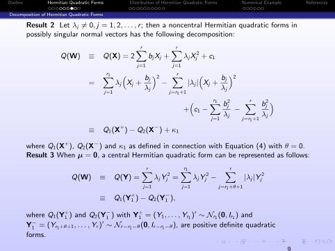
Result 2 Let λj 6= 0, j = 1, 2, . . . , r ; then a noncentral Hermitian quadratic forms inpossibly singular normal vectors has the following decomposition:

Q(W) ≡ Q(X) = 2r∑

j=1

bjXj +r∑

j=1

λjX2j + c1

=

r1∑j=1

λj

(Xj +

bjλj

)2−

r∑j=r1+1

|λj |(Xj +

bjλj

)2+(c1 −

r1∑j=1

b2j

λj−

r∑j=r1+1

b2j

λj

)≡ Q1(X+)− Q2(X−) + κ1

where Q1(X+), Q2(X−) and κ1 as defined in connection with Equation (4) with θ = 0.Result 3 When µ = 0, a central Hermitian quadratic form can be represented as follows:

Q(W) ≡ Q(Y) =r∑

j=1

λjY2j =

r1∑j=1

λjY2j −

r∑j=r1+θ+1

|λj |Y 2j

≡ Q1(Y+1 )− Q2(Y−1 ),

where Q1(Y+1 ) and Q2(Y−1 ) with Y+

1 = (Y1, . . . ,Yr1)′ ∼ Nr1(0, Ir1) and

Y−1 = (Yr1+θ+1, . . . ,Yr )′ ∼ Nr−r1−θ(0, Ir−r1−θ), are positive definite quadratic

forms.

9



Result 4 When µ = 0, C = 0 and the covariance matrix Γ is Hermitian andnon-negative definite (possibly singular), the eigenvalues of B ′H1B occur inpairs. In this case, the exact density function of Q(W) can be determined.Result 5 When the matrix H1 is positive semidefinite, so is Q, and then,Q ∼ Q1 + T .

Result 6 In the real case, let Q(U) = U′AU be a quadratic form where

U ∼ Nn(µ,Σ), the rank of Σ is r ≤ n and A = A′. Suppose U = BZ +µ where

we redefine Bn×r to be such that Σ = BB ′ and Z ∼ Nn(0, In). On replacing H1

by A in Equation (3) and letting b′ = µ′ABP, one can make use of Equation

(4) to obtain a decomposition of a noncentral real quadratic forms in possibly

singular normal vectors in terms of the difference of two positive definite

quadratic forms and an independently distributed normal random variable.

10


Hermitian Quadratic Expression

Hermitian Quadratic Expression: Let Q∗(W) = W′HW + 1

2W′α + 1

2α′W + d be

a Hermitian quadratic expression where α′ = (a′1 + ia′2) and d is real scalarconstant. First, note that

1

2W′α +

1

2α′W =

1

2(U′ − iV′)(a1 + ia2) +

1

2(a′1 − ia′2)(U + iV)

= a1U + a2V = (a′1, a′2)

(UV

)= (a′1, a

′2)

[B

(Z1

Z2

)+

(µu

µv

)]= a(BZ + µ) (5)

where a = (a′1, a′2). Now, on making use of Equations (3) and (5), the following

decomposition of Q∗(W) is obtained:

Q∗(W) = µ′H1µ + 2µ′H1 BZ + Z′B ′H1BZ + a(BZ + µ) + d

= Z′B ′H1BZ + 2(µ′H1 +1

2a)BZ + µ′H1µ + aµ + d (6)

Now, on letting b′1 = (µ′H1 + 12a)BP and c2 = µ′H1µ + aµ + d and following

the steps leading to Equation (4), one can represent a noncentral Hermitian

quadratic expression in possibly singular normal vectors in terms of the

difference of two positive definite quadratic forms and an independently

distributed normal random variable.11


Cumulants Generating Function, Cumulant and Moments

The Moment Generating Function of a Hermitian QuadraticExpression: Let Q∗(W) = W

′HW + 1

2W′α + 1

2α′W + d and Q(W) = W

′HW

respectively be a Hermitian quadratic expression and a Hermitian quadratic formwhere W ∼ CN n(µW , Γ,C), µW = µu + iµv, C is symmetric and Γ and H areHermitian, with Γ and C possibly singular, α′ = (a′1 + ia′2) and d is real scalarconstant. First on expressing Q∗(W) and Q(W) in terms of real quantities as wasdone in Equations (6) and (3), one can make use of the moment generatingfunctions of Q∗(W) and Q(W) as derived in Mathai and Provost (1992):

MQ∗(t) = |Ir − 2tB ′H1B|−12 exp{t(µ′H1µ + a′µ + d)

+t2

2(B ′a + 2B ′H1µ)′(I − 2tB ′H1B)−1(B ′a + 2B ′H1µ)} (7)

which on letting a = 0′ and d = 0, becomes

MQ(t) = |Ir − 2tB ′H1B|−1/2 exp{tµ′H1µ + 2t2µ′H1B

+(I − 2tB ′H1B)−1B ′H1µ}

where H1 is a real symmetric 2n × 2n matrix, a = (a′1, a′2), Σ = BB ′ of rank r ≤ 2n,

B is 2n × r of rank r and B ′H1B 6= O. Alternatively,

MQ(t) ={ r∏

j=1

(1− 2tλj)− 1

2

}exp{c1t + 2t2

r∑j=1

b2j (1− 2tλj)

−1}, µ 6= 0

=r∏

j=1

(1− 2tλj)− 1

2 , µ = 0 (8)

λ1, . . . , λp being the eigenvalues of B ′H1B, B ′H1B 6= O , c1 = µ′H1µ,

b′ = P ′B ′H1µ, PP ′ = I .12



Cumulants: If lnMQ∗(t) admits a power series expansion, then the coefficient ofts/s! is defined as the sth cumulant of W denoted by k∗(s). That is,lnMQ∗(t) =

∑∞s=1 k

∗(s) ts

s!. If lnMQ∗(t) is differentiable then

k∗(s) = ds

dts[lnMQ∗(t)]|t=0.

One can determine the cumulant generating function (cgf) of Q∗(W) as follows fromEquation (7):

lnMQ∗(t) = −1

2ln|Ir − 2tB ′H1B|+ t(d + a′µ + µ′H1µ)

+t2

2(B ′a + 2B ′H1µ)′(Ir − 2tB ′H1B)−1(B ′a + 2B ′H1µ).

(9)

Moreover, the cumulant generating function of Q(W) can be determined as followsby making use of Equation (8):

lnMQ(t) = −1

2

r∑j=1

ln(1− 2tλj) + c1t + 2t2r∑

j=1

b2j

(1− 2tλj). (10)

13



Alternatively, one can determine the cgf of Q(W) = Q1(X+)− Q2(X−) + T asfollows. First,

Q† = X+A1X+ − X−A2X

− = X′AX

where A =

(A1 OO A2

)and X′ = (X+ , X−)′ ∼ N2r (ν

∗, I2r ), with

ν∗ = (ν′1,ν′2)′, ν1 and ν2 being as defined in Equation (4). On making use of

(10), one can determine the cumulant generating function of Q† as

lnMQ†(t) = −1

2

r∑j=1

ln(1− 2tλ∗j ) + c2t + 2t2r∑

j=1

δ2j(1− 2tλ∗j )

(11)

where P1 is an 2r × 2r orthogonal matrix such that P ′1B′1AB1P1 = Diag(λ∗1 ,

. . . , λ∗2r ), λ∗1 , . . . , λ∗2r are the eigenvalues of B ′1AB1,

δ′ = (δ1, . . . , δ2r ) = ν′AB1P1, c2 = ν′Aν and I2r = B ′1B1.The cgf of T ∼ N (κ1 , 4

∑r1+θj=r1+1 b

2j ) whose parameters are as defined in

Equation (4), is κ1t + σ2t2/2 where σ2 = 4∑r1+θ

j=r1+1 b2j . Since Q† and T are

independent, then

lnMQ(t) = lnMQ†+T (t) = lnMQ†(t) + lnMT (t)

= −1

2

2r∑j=1

ln(1− 2tλ∗j ) + c2t + 2t22r∑j=1

δ2j(1− 2tλ∗j )

+ κ1t + σ2t2/2.

(12)

14



The sth cumulant of Q∗ is

k∗(s) = 2s−1s!{

(1/s)tr(B ′H1B)s + (1/4)a′B(B ′H1B)s−2B ′a

+ µ′H1B(B ′H1B)s−2B ′H1µ + a′B(B ′H1B)s−2B ′H1µ}

for s ≥ 2

= tr(B ′AB) + µ′Aµ + a′µ + d for s = 1 (13)

Alternatively, the sth cumulant of Q(W) = W′H1W can be expressed as

k(s) = 2s−1s!

p∑j=1

λsj (b

2j + 1/s) (14)

where λ1, . . . , λp are the eigenvalues of Σ12H1Σ

12 , b′ = (b1, . . . , b2n) = (P ′Σ−

12µ)′ and

θs =∑p

j=1 λsj (s b

2j + 1), s = 1, 2, . . . . Note that tr(H1Σ)h =

∑2nj=1 λ

sj .

One can also make use of Equation (12) to obtain another representation of k(s):

k(s) = 2s−1s!2r∑j=1

(λ∗j )s(δ2j + 1/s) for s ≥ 3

= 2s−1s!2r∑j=1

(λ∗j )s(δ2j + 1/s) + σ2 for s = 2

= 2s−1s!2r∑j=1

(λ∗j )s(δ2j + 1/s) + κ1 + σ2t for s = 1 (15)

where σ, κ1, λ∗j and δ are as defined in (12).15



Recursive relationship between cumulants and momentsIn general, the moments of a random variable can be obtained from itscumulants by means of a recursive relationship given in Smith (1995),which can also be deduced for instance from Theorem 3.2b.2 of Mathaiand Provost (1992). Accordingly, the sth moment of Q∗(X) can beobtained as follows:

µ∗(s) =s−1∑i=0

(s − 1)!

(s − 1− i)! i !k∗(s − i)µ∗(i) , (16)

where k∗(s) is as specified in (13).

16


The Exact Density of a Central Hermitian Quadratic Form

The Exact Density of a Central Hermitian Quadratic Form Whenthe Eigenvalues Occur in Pairs: In this case, Q(W) can be expressedas

Q(W) =s∑

i=1

λ′i Ti −t∑

j=s+1

|λ′j |Tj ,

where s = r/2, t = p/2, λ′k = λk/2, k = 1, . . . , t, and the Ti ’s and Tj ’sare independently distributed chi-square random variables, each havingtwo degrees of freedom. Imhof (1961) derived the followingrepresentation of the exact density function of Q(W)

g(q) =

∑sj=1

(λ′j )t−2 e

−q/(2λ′j )

2

(∏sk=1,k 6=j (λ

′j−λ

′k )

)(∏tk=s+1(|λ′j |+|λ

′k |)) , q ≥ 0

∑tj=s+1

|λ′j |t−2 e

q/(2|λ′j |)

2

(∏tk=s+1,k 6=j (|λ′j |−|λ

′k |))(∏s

k=1(λ′j+λ′k )

) , q < 0.

(17)

17


Approximations by Means of Gamma Distribution

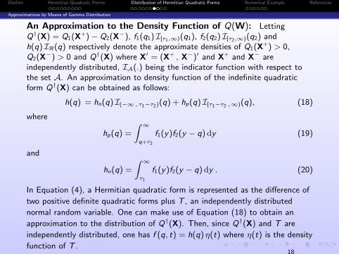
An Approximation to the Density Function of Q(W): LettingQ†(X) = Q1(X+)− Q2(X−), f1(q1) I[τ1,∞)(q1), f2(q2) I[τ2,∞)(q2) andh(q) I<(q) respectively denote the approximate densities of Q1(X+) > 0,Q2(X−) > 0 and Q†(X) where X′ = (X+ , X−)′ and X+ and X− areindependently distributed, IA(.) being the indicator function with respect tothe set A. An approximation to density function of the indefinite quadraticform Q†(X) can be obtained as follows:

h(q) = hn(q) I(−∞ , τ1−τ2)(q) + hp(q) I[τ1−τ2 ,∞)(q), (18)

where

hp(q) =

∫ ∞q+τ2

f1(y)f2(y − q)dy (19)

and

hn(q) =

∫ ∞τ1

f1(y)f2(y − q)dy . (20)

In Equation (4), a Hermitian quadratic form is represented as the difference of

two positive definite quadratic forms plus T , an independently distributed

normal random variable. One can make use of Equation (18) to obtain an

approximation to the distribution of Q†(X). Then, since Q†(X) and T are

independently distributed, one has f (q, t) = h(q) η(t) where η(t) is the density

function of T .18


Approximations by Means of Gamma Distribution

In order to determine an approximation to the distribution of V = Q†(X) + T ,it suffices to apply transformation of variables technique. Letting U = T , thejoint density function of U and V is g(v , u) = f (v − u , u)|J| where J is theJacobian of the inverse transformation. Thus, the density function of V is

s(v) =

∫ ∞−∞

g(v , u) du . (21)

Gamma approximations are appropriate to approximate the density function ofnoncentral quadratic forms. The gamma density function is given by

ψ(x) =xα−1e−x/β

Γ(α)βαI[0,∞)(x) , for α > 0 and β > 0. (22)

Let the raw moments of a noncentral quadratic form be denoted by µj ,j = 1, 2, . . . ; then, a gamma approximation can obtained by equating the firsttwo moments associated with (22) to µ1 and µ2, respectively, and evaluating αand β. In this case, αβ = µ1 and α(α + 1)β2 = µ2, which yields

α =µ21

µ2 − µ21

, β =µ2

µ1− µ1.

19


Polynomially Adjusted Density Functions

Polynomially Adjusted Density Functions: On the basis of the first nmoments of the quadratic form, Q(W), a density approximation of thefollowing form is assumed for Q(W):

fn(x) = ψ(x)n∑

j=0

ξj xj

where ψ(x) is an initial density approximant referred to as base densityfunction. In order to determine the polynomial coefficients, ξj , we equatethe sth moment of Q(W) to the sth moment of the approximatedistribution specified by fn(x) for s = 0, 1, . . . , n. That is,

µQ1(s) =

∫ ∞τ1

x sψ(x)n∑

j=0

ξjxjdx =

n∑j=0

ξj

∫ ∞τ1

x s+jψ(x)dx

=n∑

j=0

ξj ms+j , s = 0, 1, . . . , n,

where ms+j is the (s + j)th moment determined from ψ(x).

20


Polynomially Adjusted Density Functions

This leads to a linear system of (n + 1) equations in (n + 1) unknownswhose solution is

ξ0ξ1...ξn

=

m0 m1 · · · mn

m1 m2 · · · mn+1

· · · · · · · · · · · ·mn mn+1 · · · m2n

−1

µ(1)0

µ(1)1...

µ(1)n

.

The resulting representation of the density function of Q1(X) will bereferred to as a polynomially adjusted density approximant, which can bereadily evaluated. As long as higher moments are available and thecalculations can be carried out with sufficient precision, more accurateapproximations can be obtained by making use of additional moments.The density function of Q2(X) can be approximated by making use of thesame procedure. An approximate density for Q1(X)− Q2(X) can then beobtained via Equation (18).

21


Example 1

Example 1: Let Q(W) = W′HW where W = X1 + iY1 ∼ CN n(0, Γ,O) and

Γ =

(1 3i/2

−3i/2 4

), H =

(2 1− i

1 + i −6

).

By making use of Equation (3), one can represent Q(W) as the following realquadratic from:

Q(W) = (X′1 , Y′1)H1

(X1

Y1

)(23)

where

G =

(1 1.5i0 1.323

)and H1 =

2 1 0 11 −6 −1 00 −1 2 11 0 1 −6

.

Moreover, one has

(X1

Y1

)∼ N2n

(µW,Σ

)where µ′W = (0′, 0′) and

Σ =1

2

1 0 0 −3/20 4 3/2 00 3/2 1 0−3/2 0 0 4

22


Example 1

The eigenvalues of G ′1H1G1 where G1 is the symmetric square root of Σ, are(−12.9722, −12.9722, 0.472165, 0.472165). Since the eigenvalues occur in pairs, onecan apply Equation (17) to obtain the exact distribution function of Q(W). Certainexact percentiles are presented in the following table. Additionally, the approximatepercentiles obtained from the gamma distribution with polynomial adjustments ofdegree 10 are also tabulated. The results show that these approximations are veryaccurate.

Table: Exact cdf’s and polynomially adjusted gamma approximations (d = 10) to thedistribution function of Q(W) evaluated at certain percentage points

CDF Exact Gamma-Poly0.0001 -238.029 0.00010.001 -178.29 0.0010.01 -118.551 0.010.05 -76.7947 0.050.50 -17.0557 0.500.95 -0.403221 0.950.99 1.18625 0.989999

0.999 3.36065 0.9990.9999 5.53505 0.9999

23


Example 2

Example 2:Let Q∗(W) = W

′HW + 1

2W′α + 1

2α′W + d where W ∼ CN n(µW, Γ,C),

µW = (1 + 2i , 3 + 4i , 2.1 + 3i ,−3− 1.4i)′,α = (1− 2i , 2 + 1.2i ,−1 + 3i ,−5− 4i)′, d = 4,

Γ =

10 1 + i i 2− 2i

1− i 18 1 + i 1 + 3i−i 1− i 13 −i

2 + 2i 1− 3i i 14

and

H =

2 2 i 22 2 i 2−i −i 4 1 + 2.5i2 2 1− 2.5i −10

C =

1 0.3 1 1

0.3 2.3 1.7 11 1.7 2.3 21 1 2 2.3

.

By making use of Equation (6), one can represent Q∗(W) as the following realquadratic from:

Q(W) = (X′1 , Y′1)H1

(X1

Y1

)+ a

(X1

Y1

)+ d

24


Example 2

where

H1 =

2 2 0 2 0 0 −1 02 2 0 2 0 0 −1 00 0 4 1 1 1 0 −2.52 2 1 −10 0 0 2.5 00 0 1 0 2 2 0 20 0 1 0 2 2 0 2−1 −1 0 2.5 0 0 4 10 0 −2.5 0 2 2 1 −10

,

a′ = (1, 2,−1,−5,−2, 1.2, 3,−4) and

(X1

Y1

)∼ N2n

(µ,Σ

)where

µ′ = (1, 3, 2.1,−3, 2, 4, 3,−1.4) and

Σ =

11 1.3 1 3 0 −1 −1 21.3 20.3 2.7 2 1 0 −1 −31 2.7 15.3 2 1 1 0 13 2 2 16.3 −2 3 −1 00 1 1 −2 9 0.7 −1 1−1 0 1 3 0.7 15.7 −0.7 0−1 −1 0 −1 −1 −0.7 10.7 −22 −3 1 0 1 0 −2 11.7

.

25


Example 2

The eigenvalues of Σ1/2H1Σ1/2 where Σ1/2 is the symmetric square rootof Σ, are −81.732,−65.954, 50.969, 37.379, 24.819, 17.519, 0 and 0. Theapproximate cdf obtained from the gamma distribution with polynomialadjustments of degree 10 was evaluated at certain percentile of thedistribution in the following table. The results suggest that theseapproximations are very accurate.

Table: Polynomially adjusted gamma approximations (d = 10) to thedistribution function of Q∗(W) evaluated at certain percentage points obtainedby simulation

CDF Simulated Gamma-Poly0.01 -1133.3 0.0101910.05 -720.23 0.0496090.10 -530.17 0.0983330.50 -19.165 0.5002050.90 346.60 0.8996860.95 465.09 0.9501830.99 717.75 0.989654

26


Example 2

Simulated CDF and Gamma-Polynomial CDFApproximation

27


References:

Imhof, J. P. (1961).Computing the distribution of quadratic forms in normal variables,Biometrika,48, 419–426.

Mathai, A. M., Provost, S. B.,, E. M. (1992).Quadratic Forms in Random Variables, Theory and Applications.Marcel Dekker Inc., New York.

Smith, P. J. (1995).A recursive formulation of the old problem of obtaining moments fromcumulants and vice versa,The American Statistician,49, 217–219.

27


Thanks

28

on approximating of the distribution of · pdf fileoutline hermitian quadratic forms...

Documents