On a two-sector endogenous growth model with

quasi-geometric discounting

Ryoji Hiraguchi∗†

June 29, 2012

Abstract

This article studies a two-sector endogenous growth model with quasi-geometric

discounting. We first specialize to log utility and derive a recursive equilibrium

path and a planner’s solution path. We find that if the discount factor is close

to 1, the planner’s solution welfare-dominates the equilibrium path. Our result

contrasts with the results in Krusell, Kuruscu, and Smith (Journal of Economic

Theory, 2002) who study the Ramsey model to show that the competitive economy

always outperforms the planned economy. We next show that if the utility function

demonstrates constant relative risk aversion, there can be multiple balanced growth

paths.

Keywords: endogenous growth; quasi-geometric discounting; time consistency

JEL classification: E5;

∗Faculty of Economics, Ritsumeikan University, 1-1-1, Noji-higashi, Kusatsu, Shiga, Japan. Tel: 81-

77-561-4837. Fax: 81-77-561-4837.†Email: rhira@fc.ritsumei.ac.jp

1

1 Introduction

Experimental evidence suggests that discounting of future rewards is not geometric (Thaler,

1981; Benzion et al., 1989). Economic models of time-inconsistent preferences are initially

studied by Strotz (1956), Phelps and Pollak (1968), and Pollak (1968). Laibson (1997) and

Barro (1999) reformulate these models by adopting quasi-geometric (quasi-hyperbolic) dis-

counting. Although some authors (Rubinstein, 2003; Schwarz and Sheshinski, 2007) argue

that quasi-geometric discounting is controversial from an empirical viewpoint, Salois and

Moss (2011) use market asset data and obtain a statistically significant quasi-geometric

parameter.

An important study by Krusell, Kuruscu, and Smith (2002) (henceforth KKS) in-

troduces quasi-geometric discounting into the standard discrete-time neoclassical growth

model. KKS solve an individual’s problem as a game between current-self and future-self

and focus on Markov equilibria in which only current state variables affect an individual’s

behavior. Surprisingly, they show that the recursive competitive equilibrium path always

welfare-dominates the social planner’s solution path. Moreover, they perform a numerical

analysis to find that the competitive equilibrium is uniquely determined for a general class

of utility functions (KKS, p.48, line 28).

Their results, however, are based on the assumption of only one sector in the economy.

This paper examines whether their results hold in a two-sector economy. The set-up is

almost the same as in KKS. The only difference is that production of the final good

requires human as well as physical capital. The individual has a unit time endowment

that is allocated between working (i.e., final goods production) and studying (i.e., human

capital accumulation).

First we derive the recursive competitive equilibrium path and the planner’s solution

path explicitly. Following KKS, we specialize to log period utility and assume that phys-

ical and human capitals depreciate completely. We find that the two paths converge to

different balanced growth paths. We then compare the competitive equilibrium path with

the planner’s solution path in terms of social welfare and show that when the discount fac-

tor is sufficiently close to 1, the planner’s solution path welfare-dominates the equilibrium

2

path. This result differs from KKS.

The crucial difference between our model and KKS is that the welfare function (i.e.,

the intertemporal utility at date 0) in our model depends both on the savings rate and

working time, whereas in the one-sector economy of KKS, welfare depends only on the

latter and working time is fixed. (It is shown that these two variables are constant for

both the competitive economy and the planned economy.) As in KKS, the savings rate

in the competitive economy is closer to the welfare-maximizing savings rate than in the

planned economy. Thus the competitive equilibrium would welfare-dominate the planner’s

solution path if working time is the same in both economies. However, working time in

the competitive economy is actually farther from the welfare-maximizing working time

than in the planned economy. Therefore, the planned economy performs better than the

competitive economy for some parameter values.

When preferences are quasi-geometric, the solution path chosen by the social planner

generally differs from the competitive equilibrium path. Moreover, even the benevolent

planner cannot choose the savings rate and working time that maximize social welfare,

because such a strategy is shown to be time inconsistent. This is the reason why the

planned economy may perform better or worse than the competitive economy.

Next we use a general constant relative risk aversion (CRRA) utility function and

characterize the balanced growth path. Here we focus on the stationary competitive equi-

librium path because, as KKS point out, deriving the optimal path becomes analytically

difficult when we abandon the log preferences. We find that when the coefficient of relative

risk aversion is less than 1, two balanced growth equilibria are possible. This result con-

trasts with results in KKS. The multiplicity result is also obtained by Krusell and Smith

(2003), who show that the neoclassical growth model with quasi-geometric discounting

has a continuum of solution paths. One difference between Krusell and Smith (2003) and

our paper is that they investigate the planned economy whereas we study the competitive

economy.

The quasi-geometric discounting function is now applied to many fields of economics,

particularly macroeconomics. Laibson (2001) argues that quasi-geometric discounting

3

leads to under-saving, whereas Salanie and Treich (2006) show that the result can be

opposite for some classes of utility functions. Diamond and Koszegi (2003) show that

workers with quasi-geometric discounting retire early. Schwarz and Sheshinski (2007)

investigate social security issues. Maliar and Maliar (2006) find indeterminate results.

However, these papers are based on either partial equilibrium models or on standard

one-sector models. To our knowledge, no previous paper investigates quasi-geometric

discounting in a multi-sector economy.

There has been a long debate about whether human capital accumulation enhances

economic growth. Whereas earlier empirical works argue that increases in education

are not significantly connected with economic growth (Mankiw, Romer, and Weil, 1992;

Bils and Klenow, 2000), more recent literature finds a link. For example, Cohen and

Soto (2007) construct a comparative multinational dataset for years of schooling and

show that schooling contributes to economic growth even after controlling for physical

capital accumulation. Ciccone and Papaioannou (2009) obtain similar results. These

findings suggest the importance of studying models in which human capital accumulation

is explicitly described.

Two-sector endogenous growth models were initiated by Uzawa (1965) and developed

by Lucas (1988). Numerous extensions have followed these pioneering works. Caballe

and Santos (1993) investigate the transitional dynamics. Benhabib and Perli (1994) in-

corporate human capital externalities into the model and find that the optimal path

can be locally indeterminate. Bond, Wang, and Yip (1996) investigate the case where

physical capital is needed in both final goods production and human capital accumula-

tion. Ladron-de-Guevara, Ortigueira, and Santos (1996) introduce labor-leisure choice

into the model and find multiple balanced growth paths. Jones, Manuelli, and Rossi

(1993); Garcia-Castrillo and Sanso (2000); Gomez (2002); and Garcıa-Belenguer (2007)

study fiscal policy issues. However, each of these papers uses geometric discounting.

This paper is organized as follows. Section 2 describes the model. Section 3 studies an

equilibrium path. Section 4 examines a planner’s solution. Section 5 studies the equilib-

rium multiplicity. Section 6 concludes. The Appendix presents proofs of the propositions.

4

2 The environment

The environment in this paper extends that of KKS to allow for human capital accu-

mulation. Time is discrete and ranges from 0 to +∞. Preferences of the representative

individual at the beginning of period 0 are given by U0 = u0 + β(δu1 + δ2u2 + ...), where

ut is the utility in period t, δ ∈ (0, 1) is the discount factor, and β > 0 shows the degree

of time inconsistency. If β < 1 (β > 1), the individual is present biased (future biased).

Following KKS, we treat the individual’s problem as a game between the current self and

the future self and focus on Markov equilibria in which only current state variables mat-

ter. For the time being, we assume that period utility takes the simple form u(c) = ln(c).

Intertemporal utility reduces to U0 = ln c0 + β∑∞

t=0 δt ln ct.

The individual has a unit time endowment. He spends nt units producing final goods

and 1 − nt units on human capital accumulation. The feasible allocation must satisfy

nt ∈ [0, 1]. In the following, we simply call nt ”working time.” The production function

is Cobb-Douglas, and the resource constraint is given by

kt+1 = Akαt (ntht)

1−α − ct for t ≥ 0, (1)

where kt is the stock of physical capital in period t, A > 0 is the productivity parameter,

α ∈ (0, 1) is the physical capital share, ht is the stock of human capital in period t, and

ct is consumption at time t. Physical capital is fully depreciated. The term ntht shows

efficiency per unit of labor. Evolution of human capital is governed by

ht+1 = B(1 − nt)ht for t ≥ 0, (2)

where the parameter B > 0 shows the efficiency of human capital accumulation. Moreover,

the human capital is fully depreciated.

Factor markets are perfectly competitive, and the real interest rate and the wage rate

in period t are respectively given by rt = αAkα−1t (ntht)

1−α and wt = (1−α)Akαt (ntht)

−α.

5

3 Recursive competitive equilibrium

In this section, we obtain the recursive competitive equilibrium path. Let x ≡ (k, h) ∈ R2+

denote a vector of the state variables. Variables with primes show next-period values. For

example, k′ denotes the value of physical capital in the next period.

3.1 Definition of the equilibrium

The individual chooses his future state x′ by assuming that factor prices r(x) and w(x)

depend on the aggregate state x = (k, h) and that the process of x, x′ = G(x) =

(G1(x), G2(x)) and his future decision rule x′ = g(x, x) = (g1(x, x), g2(x, x)) are given.

Here G1 (G2) is the next period’s total physical (human) capital, and g1 (g2) denotes the

individual’s physical (human) capital in the next period. (Note that g, G : R2+ → R2

+.)

The individual’s budget constraint is k′ = r(x)k + w(x)nh − c, and human capital

accumulation is according to h′ = B(1−n)h, which is re-written as n = 1−h′/(Bh). The

set-up follows Garcıa-Belenguer (2007). The rule g determines his consumption c(x, x)

and working time n(x, x), that depend on his state x and the aggregate state x:

c(x, x) = r(x)k + w(x)

{1 − g2(x, x)

Bh

}h − g1(x, x), (3)

n(x, x) = 1 − g2(x, x)

Bh. (4)

The current self’s problem, say P1, is

(P1) V e0 (x, x) = max

c≥0,n∈[0,1][ln c + βδV e(x′, x′)] , (5)

s.t. k′ = r(x)k + w(x)nh − c, (6)

h′ = B(1 − n)h. (7)

The value function V e(x, x) satisfies the functional equation (hereafter FE)

FE: V e(x, x) = ln(c(x, x)) + δV e(g(x, x), G(x)), (8)

6

and the terminal condition (hereafter TC)

TC: limT→∞

δT V e(xT , xT ) = 0, (9)

where the sequence xt = (kt, ht) is defined as x0 = (k, h) and xt = g(xt−1, xt−1) for t ≥ 1.

Before proceeding, we comment on the terminal condition (9) that KKS do not impose.

Iterations of Eq. (8) yield

V e(x, x) =T∑

t=0

δt ln(c(xt, xt)) + δT+1V e(xT+1, xT+1),

for any T ≥ 0. To assure that V e is the correct value function, the second term on the

right-hand side (RHS) of the above equation must go to 0 as t goes to infinity as Stokey,

Lucas, and Prescott (1989) point out. Thus, we need Eq. (9). Its satisfaction is not

obvious because the economy grows in our model and V (xt) diverges as t goes to infinity.

We formally define the recursive competitive equilibrium.

Definition 1: A recursive competitive equilibrium consists of a decision rule g(x, x) ,

a value function V (x, x), factor prices r(x) and w(x), and a difference equation on the

aggregate state x′ = G(x) such that

1. given V (x, x), the decision rule g(x, x) solves the problem P1;

2. given g(x, x), the value function V (x, x) satisfies the FE (8) and the TC (9);

3. r(x) = αAkα−1(n(x, x)h)1−α and w(x) = (1 − α)Akα(n(x, x)h)−α; and

4. G(x) = g(x, x).

With regard to the first condition of Definition 1, the original problem P1 is to choose

the current control variables c and n, not the future state variables g. However, we can

easily confirm there is a one-to-one relationship between the current control variables (i.e.,

c and n) the future state variables (i.e., k′ and h). Thus, when c(x, x) and n(x, x) solve

P1, we say that the rule g(x, x) solves P1. The fourth condition implies that aggregate

capital accumulation is consistent with the individual’s capital accumulation.

7

3.2 Characterization

To obtain the equilibrium path, we first substitute Eq. (7) into Eq. (6) and obtain a

consolidated budget constraint k′ + (w(x)/B)h′ = r(x)k + w(x)h − c. It shows that the

rate of return on physical capital in period t is r(x′) and the return on human capital

is Bw(x′)/w(x). To guarantee existence of the equilibrium, the non-arbitrage condition

between physical and human capital must hold. 1 Thus we have

r(xt+1)w(xt) = Bw(xt+1) for all t ≥ 0. (10)

Under Eq. (10), the choice of n is irrelevant to the individual’s utility, and the consolidated

budget constraint is simplified as y(x′, x′) = r(x′){y(x, x)− c}, where y(x, x) = r(x)k +

w(x)h is the market value of the individual’s total personal capital. We have

Proposition 1 The recursive equilibrium is given by

1. G(x) = [seAkα(neh)1−α, B(1−ne)h], where se = αδβ/(1−δ+δβ) is the equilibrium

savings rate and ne = (1 − δ)/(1 − δ + δβ) is the equilibrium working time;

2. g(x, x) = [(1 − ne)r(x)k, (1 − ne)Bh]; and

3. V e(x, x) = p1 ln(r(x)k + w(x)h) + p2 ln r(x) + p3, where p1 = 1/(1 − δ), p2 =

αδ/{(1 − δ)(1 − αδ)} and p3 = { ln ne + δp1 ln(1 − ne) + δ(p1 + p2) ln(B1−α)}/(1 − δ).

Proof. See the Appendix.

Let {ket , h

et , c

et}∞t=0 denote the equilibrium allocation where ke

t , het and ce

t respectively

denote physical capital, human capital, and consumption in period t. It satisfies ket+1 =

seAkαt (neht)

1−α, het+1 = B(1 − ne)he

t and cet = (1 − se)Akα

t (neht)1−α. Thus, the human

capital growth rate Γe = δβB/(1 − δ + δβ) is constant, and as t goes to infinity, the

growth rates of physical capital and output converge to Γe. The balanced growth rate Γe

decreases with β, that is, the more future-biased the individual is, the less time he spends

1If r(x′) < Bw(x′)/w(x), each individual spends all his time on human capital accumulation (i.e.,

n = 0). In this case, total output in period t is zero, and positive consumption is impossible because

physical capital is fully depreciated. On the other hand, if r(x′) > Bw(x′)/w(x), the individual chooses

n = 1, and human capital (and output) will be zero tomorrow.

8

producing final goods and the more the economy grows.

4 Planning problem

Now, we investigate the problem of benevolent government. Following KKS, we assume

that the preferences of the planner are the same as those of the current self, and we look for

a time-consistent solution path to the planning problem. Suppose the current self perceives

its future decision on physical and human capital is embodied by g∗(x) = (g∗1(x), g∗

2(x)),

where g∗1 (g∗

2) denotes the next period’s physical (human) capital. The rule g∗ uniquely

determines the decision rules for consumption and working time as

c∗(x) = Akα{h − B−1g∗2(x)}1−α − g∗

1(x), (11)

n∗(x) = 1 − (Bh)−1g∗2(x). (12)

Let P2 denote the problem of the planner’s current self. It is given by

(P2) V ∗0 (x) = max

c,n[ln(c) + βδV ∗(x′)] ,

s.t. k′ = Akα(nh)1−α − c and h′ = B(1 − n)h.

The value function V ∗ satisfies

FE : V ∗(x) = ln[c∗(x)] + δV ∗(g∗(x)), (13)

TC : limt→∞

δtV (g∗(t)(x)) = 0, (14)

where a sequence of the function {g∗(t)(x)}∞t=0 is defined by g∗(t+1)(x) = g[g∗(t)(x)] for

t ≥ 0 and g∗(0)(x) = x. We formally define the planner’s solution.

Definition 2: A solution to the planner’s problem consists of a decision rule g∗(x) (=

(g∗1(x), g∗

2(x))) and a value function V ∗(x) such that

1. given V ∗(x), the rule g∗(x) solves the problem (P2); and

2. given g∗(x), the value function V ∗(x) satisfies the FE (13) and the TC (14).

9

We have

Proposition 2 A solution to the planner’s problem is given by

1. g∗(x) = [s∗Akα(n∗h)1−α, B(1−n∗)h], where s∗ = βδα/{1−αδ+βδα} is the savings

rate and n∗ = (1 − αδ + βδα)(1 − δ)/{(1 − αδ + βδα)(1 − δ) + βδ} is working time; and

2. V ∗(x) = ρ1 ln k+ρ2 ln h+ ρ3 where ρ1 = α/(1−αδ), ρ2 = (1−α)/{(1−δ)(1−αδ)}and ρ3 = {(1 + δρ1) ln(An∗(1−α)) + ln(1 − s∗) + δρ1 ln s∗ + δρ2 ln(B(1 − n∗))}/(1 − δ).

Proof. See the Appendix.

Let {k∗t , h

∗t , c

∗t}∞t=0 denote a solution path to the planner’s problem where k∗

t , h∗t , and

c∗t are period-t physical capital, human capital, and consumption, respectively. It satisfies

k∗t+1 = s∗A(k∗

t )α(n∗h∗

t )1−α, h∗

t+1 = B(1 − n∗)h∗t and c∗t = (1 − s∗)A(k∗

t )α(n∗h∗

t )1−α. Thus,

human capital growth rate Γ∗ = B(1−n∗) is constant, and growth rates of physical capital

and output converge to the same value Γ∗ as time goes to infinity.

The dynamics of the planner’s solution path is very similar to the dynamics of the

equilibrium path. The two paths differ only in their savings rates and working time. The

next lemma investigates the differences.

Lemma 1 If β < 1, then se > s∗ and ne > n∗. The orders are reversed if β > 1.

Proof. See the Appendix.

Thus the individual is present-biased (i.e., β < 1), and the balanced growth rate

of the planned economy, Γ∗ = B(1 − n∗), is higher than for the competitive economy

Γe = B(1 − ne).

When discounting is geometric (β = 1), there is no time inconsistency, and the com-

petitive equilibrium allocation is the same as the planner’s solution. We can easily check

that se = s∗ = αδ, ne = n∗ = 1 − δ and Γe = Γ∗ = δB if β = 1. This coincides with the

findings of Bethmann (2007) who obtains a closed-form solution path for the discrete-time

two-sector endogenous growth model with geometric discounting (Bethmann, 2007, p. 96,

Eq (22)).

10

5 Utility comparison

Here, we compare the equilibrium path with the planner’s solution path in regard to social

welfare (i.e., utility of the current self). As the previous section made clear, the savings

rate s and working time n are constant for the two paths. The next lemma provides a

simple expression for welfare when the savings rate and working time are fixed.

Lemma 2 Define θ ≡ (1 − δ)(1 − αδ). If the initial state is x, the savings rate is s and

working time is n, the utility U0 = u0 + δ(βu1 + β2u2 + ...) is expressed as

U0(x) = θ−1f(s, n) + ψ1 ln k + ψ2 ln h, (15)

where ψ1 = α(1 − β) + αβ/(1 − αδ) and ψ2 = (1 − α)(1 − β + θ−1β). The function f is

given by

f(s, n) = φ1 ln s + φ2 ln(1 − s) + φ3 ln n + φ4 ln(1 − n) + φ5,

where φ1 = αδβ, φ2 = (1 − αδ)(1 − δ + δβ), φ3 = θψ2, φ4 = βδ(1 − α)/(1 − δ), and

φ5 = φ3/(1 − α) ln A + φ4 ln B.

Proof. See the Appendix.

Thus the difference in welfare between the competitive equilibrium and the planner’s

solution, V ∗0 (x) − V e

0 (x) = θ−1{f(s∗, n∗) − f(se, ne)} is independent of the capital level,

and the planned economy welfare-dominates the competitive economy if and only if

∆V ≡ f(s∗, n∗) − f(se, ne) > 0. (16)

Investigations of Eq. (16) are not simple. However, we can show that the planned economy

outperforms the competitive economy if the individual is sufficiently patient.

Proposition 3 If the discount factor δ is close to 1 and β = 1, the solution to the

planning problem welfare-dominates the competitive equilibrium.

Proof. See the Appendix.

11

Although there exists a savings rate sf = φ1/(φ1 + φ2) = αδβ/{β + θ(1 − β)} and a

working time nf = φ3/(φ3 +φ4) = {(1− δ)θ(1−β)+β−βδ}/{(1− δ)θ(1−β)+β} which

uniquely maximize the welfare function f(s, n), the planner cannot choose a path along

which (s, n) = (sf , nf ) because of the time inconsistency. We can check that sf > se > s∗

and ne > n∗ > nf if β < 1 and that the order is reversed if β > 1. 2 This implies that the

first-best savings rate sf is closer to the equilibrium savings rate se than the savings rate

of the planner s∗, whereas the first-best working time nf is further from the equilibrium

working time ne than the planner’s working time n∗. In regard to the savings rate, the

competitive equilibrium performs better than the planner’s solution. This is consistent

with the findings of KKS (See p. 68). In KKS, welfare depends only on the savings rate,

and the competitive economy always works better than the planned economy. However,

the planned economy performs better with regard to working time. This is why the

planner’s solution can welfare-dominate the equilibrium path in our model.

We now turn to the numerical analysis. We follow Krusell et al. (2009) and Henriksen

and Kydland (2010) and define the welfare difference as a consumption-equivalent λ that

satisfies

u(c∗0) + β

∞∑t=1

δtu(c∗t ) = u((1 + λ)ce0) + β

∞∑t=1

δtu((1 + λ)cet),

so that the planner’s solution performs better than the competitive equilibrium if and

only if λ > 0. Because we are using the log utility, the welfare difference and λ satisfy

V ∗0 −V e

0 = {1 + β/(1− δ)} ln(1 + λ). Figure 1 shows λ as a function of the degree of time

inconsistency β. Following Coibion, Gorodnichenko, and Wieland (2011), we assume that

capital share is 0.4 and the discount factor is 0.99.

The figure shows that the welfare difference is positive when β = 1. When the dis-

counting is geometric (i.e., β = 1), the competitive economy coincides with the planned

economy, so there is no welfare difference.

2If β < 1, sf/se = {β + (1 − δ)(1 − β)}/{β + θ(1 − β)} > 1. Moreover, (1 − nf )/(1 − n∗) =

{θ(1 − β) + β}/{(1 − δ)θ(1 − β) + β} > 1.

12

0

0.1

0.2

0.3

0.4

0.5

0.6

0.7

0 0.2 0.4 0.6 0.8 1 1.2 1.4

Ȝ (c

onsu

mp

tio

n e

quiv

ale

nt)

ȕ (time inconsistency parameter)

Capital share Į =0.4

Discount factor į =0.99

Fig 1. Welfare dominance of the planning economy over the competitive economy

6 Multiple balanced growth paths

So far we have assumed simple log preferences. In this section, we use a general CRRA

utility function u(c) = c1−σ/(1 − σ) with σ ≤ 1, and we focus on the balanced growth

equilibrium (BGE).

Definition 3: BGE is the recursive competitive equilibrium along which the growth rates

of consumption, output, physical capital, and human capital are the same constant.

Along the BGE, working time is constant because the growth rate of human capital is

constant. Moreover, the interest rate and wage rate are constant because of the constant

returns to scale. Thus the non-arbitrage condition (10) requires that r = B.

We first characterize the partial equilibrium in which the real interest rate r is equal to

B and the wage w is constant. The individual maximizes his utility by taking his future

13

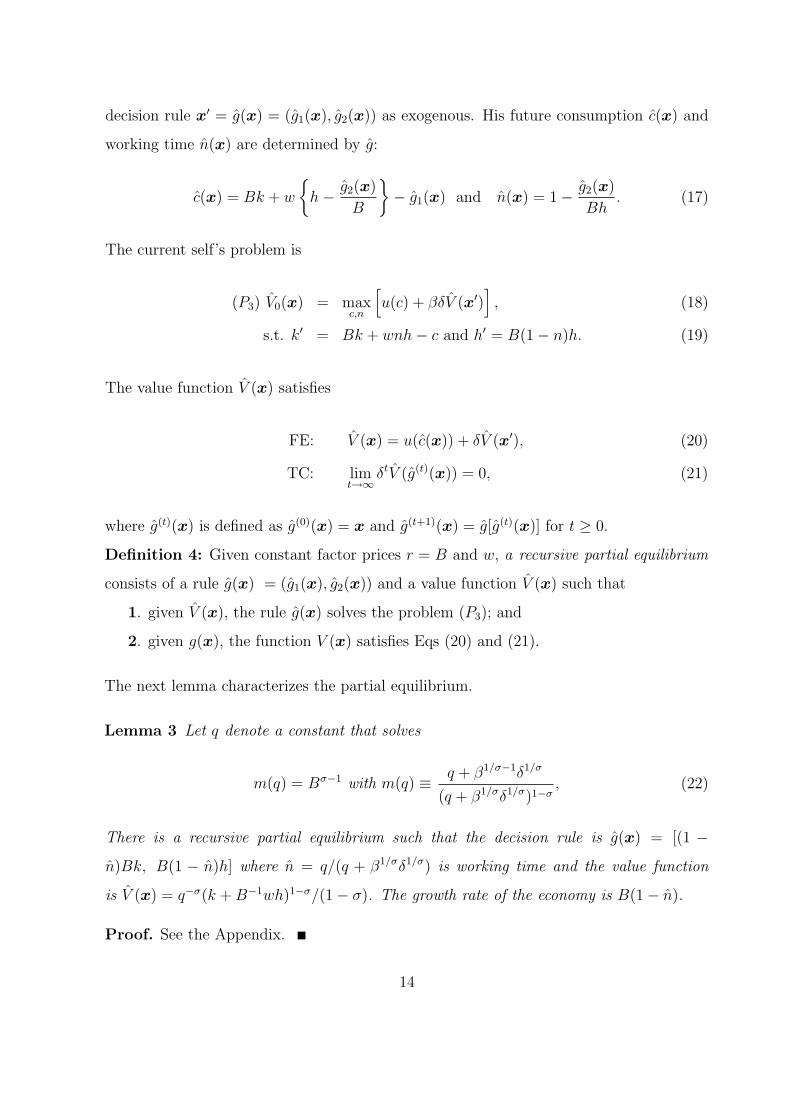
decision rule x′ = g(x) = (g1(x), g2(x)) as exogenous. His future consumption c(x) and

working time n(x) are determined by g:

c(x) = Bk + w

{h − g2(x)

B

}− g1(x) and n(x) = 1 − g2(x)

Bh. (17)

The current self’s problem is

(P3) V0(x) = maxc,n

[u(c) + βδV (x′)

], (18)

s.t. k′ = Bk + wnh − c and h′ = B(1 − n)h. (19)

The value function V (x) satisfies

FE: V (x) = u(c(x)) + δV (x′), (20)

TC: limt→∞

δtV (g(t)(x)) = 0, (21)

where g(t)(x) is defined as g(0)(x) = x and g(t+1)(x) = g[g(t)(x)] for t ≥ 0.

Definition 4: Given constant factor prices r = B and w, a recursive partial equilibrium

consists of a rule g(x) = (g1(x), g2(x)) and a value function V (x) such that

1. given V (x), the rule g(x) solves the problem (P3); and

2. given g(x), the function V (x) satisfies Eqs (20) and (21).

The next lemma characterizes the partial equilibrium.

Lemma 3 Let q denote a constant that solves

m(q) = Bσ−1 with m(q) ≡ q + β1/σ−1δ1/σ

(q + β1/σδ1/σ)1−σ, (22)

There is a recursive partial equilibrium such that the decision rule is g(x) = [(1 −n)Bk, B(1 − n)h] where n = q/(q + β1/σδ1/σ) is working time and the value function

is V (x) = q−σ(k + B−1wh)1−σ/(1 − σ). The growth rate of the economy is B(1 − n).

Proof. See the Appendix.

14

This lemma implies there are multiple recursive partial equilibria if Eq. (22) has

multiple solutions. When there is no time inconsistency (i.e., β = 1), the function m(q) =

(q + δ1/σ)σ is monotonically increasing and the solution to Eq. (22) is unique if it exists.

We have the following lemma on the shape of m when β = 1.

Lemma 4 The function m satisfies m(0) = δ and m(+∞) = +∞. If 1 − σ > β, m is

U-shaped and is minimized when q = q∗ with q∗ ≡ β−1σ−1(1 − σ − β)(βδ)1/σ > 0. If

1 − σ ≤ β, then m′(q) > 0 for all q > 0.

Proof. See the Appendix.

Lemma 2 implies that if Bσ−1 ≥ δ(= m(0)) then the solution to Eq. (22) is unique.

On the other hand, there are two solutions if the parameters satisfy β < 1 − σ and

(m(q∗) =)β1−σ(1 − β)σδ

σσ(1 − σ)1−σ< Bσ−1 < δ. (23)

Otherwise, the solution does not exist.

We have

Proposition 4 For each q satisfying Eq. (22), there exists a BGE such that

1. the initial physical and human capital satisfies

h0

k0

=1

n

(αA

B

)1/(α−1)

with n =q

q + (βδ)1/σ; (24)

2. the wage rate w(x) is constant, and the interest rate r is B;

3. the decision rule is g(x, x) = [(1 − n)Bk, B(1 − n)h];

4. the law of motion for the aggregate state is G(x) = [(1 − n)Bk, B(1 − n)h];

5. the value function is V (x, x) = q−σ(k + B−1w(x)h)1−σ/(1 − σ); and

6. the balanced growth rate is equal to B(1 − n).

If Eq. (23) holds and β < 1 − σ, two BGEs with different growth rates exist.

Proof. See the Appendix.

15

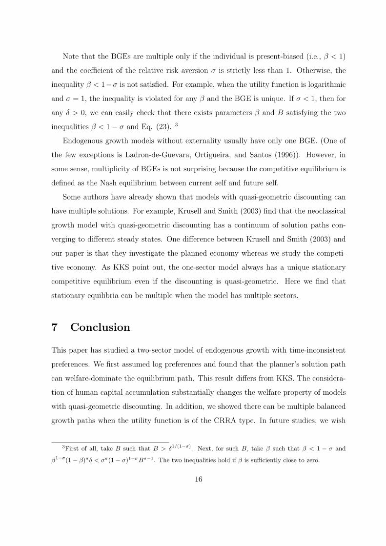
Note that the BGEs are multiple only if the individual is present-biased (i.e., β < 1)

and the coefficient of the relative risk aversion σ is strictly less than 1. Otherwise, the

inequality β < 1−σ is not satisfied. For example, when the utility function is logarithmic

and σ = 1, the inequality is violated for any β and the BGE is unique. If σ < 1, then for

any δ > 0, we can easily check that there exists parameters β and B satisfying the two

inequalities β < 1 − σ and Eq. (23). 3

Endogenous growth models without externality usually have only one BGE. (One of

the few exceptions is Ladron-de-Guevara, Ortigueira, and Santos (1996)). However, in

some sense, multiplicity of BGEs is not surprising because the competitive equilibrium is

defined as the Nash equilibrium between current self and future self.

Some authors have already shown that models with quasi-geometric discounting can

have multiple solutions. For example, Krusell and Smith (2003) find that the neoclassical

growth model with quasi-geometric discounting has a continuum of solution paths con-

verging to different steady states. One difference between Krusell and Smith (2003) and

our paper is that they investigate the planned economy whereas we study the competi-

tive economy. As KKS point out, the one-sector model always has a unique stationary

competitive equilibrium even if the discounting is quasi-geometric. Here we find that

stationary equilibria can be multiple when the model has multiple sectors.

7 Conclusion

This paper has studied a two-sector model of endogenous growth with time-inconsistent

preferences. We first assumed log preferences and found that the planner’s solution path

can welfare-dominate the equilibrium path. This result differs from KKS. The considera-

tion of human capital accumulation substantially changes the welfare property of models

with quasi-geometric discounting. In addition, we showed there can be multiple balanced

growth paths when the utility function is of the CRRA type. In future studies, we wish

3First of all, take B such that B > δ1/(1−σ). Next, for such B, take β such that β < 1 − σ and

β1−σ(1 − β)σδ < σσ(1 − σ)1−σBσ−1. The two inequalities hold if β is sufficiently close to zero.

16

to investigate a time-consistent tax policy. KKS assume that government can tax in-

come and investment proportionally and obtain the time-consistent policy equilibrium.

They find that the optimal investment tax is positive when the individual is excessively

present-biased. It will be interesting to see whether their result pertains in our two-sector

economy. In KKS, the policy equilibrium reproduces the allocation that solves the plan-

ner’s problem. This implies that time-consistent taxes always lower equilibrium welfare.

However, in our model, the planned economy can welfare-dominate the competitive econ-

omy, and we may surmise that time-consistent tax policy may improve the equilibrium

allocation.

17

Appendix

A Proof of Proposition 1

The proof is divided to five steps for clarity. For simplicity, we write w(x), w(x), r(x′),

and w(x′) as r, w, r′, and w′, respectively.

Step 1. [Given G, the non-arbitrage condition (10) holds ]: the rule G implies Bk′/h′ =

Aαkα(neh)1−α/h. This yields

r′wBw′ =

Aα(k′)α−1(neh′)1−α

B(k′)α(neh′)−αkα(neh)−α =

Aαne

B(k′/h′)kα(neh)−α = 1.

Therefore Eq. (10) holds.

Step 2. [Given g and G, V e solves the FE (8)]: it is straight forward to show that the

rule g implies n(x, x) = ne and c(x, x) = ne(rk + wh). Thus Eq. (8) holds if and only if

p1 ln(rk + wh) + p2 ln r + p3 = ln ne + ln(rk + wh) (25)

+δ[p1 ln(r′k′ + w′h′) + p2 ln r′ + p3].

Recall that given G, the non-arbitrage condition holds. The consecutive period physical

capital is k′ = rk + wneh − c(x, x) = (1 − ne)rk. Thus we get

r′k′ + w′h′ = r′(k′ +

w

Bh′

)= r′(1 − ne){rk + wh}. (26)

Because n(x, x) is time-independent, we have (r′/r)α = {(k′/h′)/(k/h)}α(α−1) = (w′/w)α−1.

Inserting this equation into Eq. (10), we have (r′/r)α = (r′/B)1−α or equivalently

ln r′ = ln(B1−α) + α ln r. (27)

18

Substitution of Eqs. (26) and (27) into Eq. (25) gives

p1 ln(rk + wh) + p2 ln r + p3 = (1 + δp1) ln(rk + wh) + δα(p1 + p2) ln r + ln ne

+δp1 ln(1 − ne) + δ(p1 + p2) ln(B1−α) + δp3.

This equality holds if and only if p1 = 1 + δp1, p2 = αδ(p1 + p2), and (1 − δ)p3 =

ln ne + δp1 ln(1 − ne) + δ(p1 + p2) ln(B1−α). The solutions are p1 = 1/(1 − δ), p2 =

αδ/{(1 − δ)(1 − αδ)}, and p3 = { ln ne + δp1 ln(1 − ne) + δ(p1 + p2) ln(B1−α)}/(1 − δ).

Step 3. [Given g and G, V e satisfies the TC (9)]: Eq. (9) holds if limt→∞ δt ln r(xt) = 0

and limt→∞ δt ln y(xt, xt) = 0. The first condition holds since limt→∞ ln r(xt) = ln B by

Eq. (27). To show the second condition, note that

ln y(x′, x′) = ln(1 − ne) + ln r′ + ln y(x, x)

by Eq. (26). Therefore, we get zt+1 = δt+1{ln(1−ne)+ln r′}+δzt where zt = δt ln y(xt, xt).

Because limt→∞ δt+1{ln(1 − ne) + ln r′} = 0, we get limt→∞ zt = 0.

Step 4. [Given V e and G, the decision rule ge solves P1]: the non-arbitrage condition

(10) implies that r′k′ + w′h′ = r′(rk + wh − c). Therefore, given the functional form of

V e, the problem P1 reduces to

maxc≥0,n∈[0,1]

[ln c +

βδ

1 − δln(rk + wh − c)

].

If we denote by (cmax, nmax) a solution to the problem above, we get cmax = ne{rk + wh}since ne = 1/(1+βδ/(1−δ)). By Eq. (10), any choice of n is optimal and then we can set

nmax = ne. In this case, next period state variables are given by k′ = rk + wneh− cmax =

(1 − ne)rk and h′ = (1 − ne)Bh. These coincide with the decision rule g.

Step 5. [The rules g and G are consistent ]: we have g1(x, x) = (1 − ne)rk = (1 −ne)Aαkα(neh)1−α and g2(x, x) = (1 − ne)Bh. Thus G(x) = g(x, x).

Thus, there exists a recursive competitive equilibrium with a decision rule g, a value

function V , and a difference equation on the aggregate state x′ = G(x). ¥

19

B Proof of Proposition 2

The proof consists of three steps.

Step 1. [Given g∗, the function V ∗(x) solves Eq. (13)]: the rule g∗ implies that the

consumption level is c∗ = (1− s∗)Ak∗α(n∗h∗)1−α. Thus V ∗ satisfies Eq. (13) if and only if

ρ1 ln k + ρ2 ln h + ρ3 = ln{(1 − s∗)Akα(n∗h)1−α}+δ{ρ1 ln{s∗Akα(n∗h)1−α} + ρ2 ln(B(1 − n∗)h) + ρ3}.

The RHS of the equation above is simplified as

RHS = (1 + δρ1)α ln k + {(1 + δρ1)(1 − α) + δρ2} ln h

+ ln(1 − s∗) + (1 + δρ1) ln A(n∗)1−α + δρ1 ln s∗ + δρ2 ln(B(1 − n∗)) + δρ3.

Eq. (13) holds for any k and h if and only if ρ1 = (1 + δρ1)α, ρ2 = (1 + δρ1)(1−α) + δρ2,

and (1 − δ)ρ3 = (1 + δρ1) ln A(n∗)1−α + ln(1 − s∗) + δρ1 ln s∗ + δρ2 ln(B(1 − n∗)). Thus

ρ1 = α/(1 − αδ) and ρ2 = (1 − α)/{(1 − δ)(1 − αδ)}.Step 2. [Given g∗, V ∗(x) satisfies Eq. (14)]: the asymptotic growth rate of human and

physical capitals, B(1−n∗) is constant. Thus limt→∞ δt ln k∗t = limt→∞ δt ln h∗

t = 0. Since

V ∗(x) = ρ1 ln k + ρ2 ln h plus constant, we get (14).

Step 3. [Given V ∗, the decision rule of the current self is g∗]: the current self maximizes

ln c + βδ{ρ1 ln(Akα(nh)1−α − c) + ρ2 ln(B(1 − n)h)} by choosing c and n. A solution to

the maximization problem above, say (c, n), is given by

c =Akα(nh)1−α

1 + βδρ1

= (1 − s∗)Akα(nh)1−α, (28)

n =1 + βδρ1

1 + βδρ1 + βδρ2

1−α

=1 − αδ(1 − β)

1 − αδ(1 − β) + βδ1−δ

= n∗. (29)

Thus the consecutive period aggregate state (k′, h′) is k′ = Akα(n∗h)1−α−c = s∗Akα(n∗h)1−α

and h′ = B(1 − n∗). It coincides with the decision rule g∗.

Thus a planner’s solution exists with a decision rule g∗ and a value function V ∗. ¥

20

C Proof of Lemma 1

First, with respect to the savings rates, one has

se

s∗=

1 − αδ + βδα

1 − δ + δβ=

β + (1 − β)(1 − αδ)

β + (1 − β)(1 − δ).

Because 0 < 1 − δ < 1 − αδ < 1, se/s∗ is greater than one if and only if β < 1.

Next, concerning working time, one has 1 − ne = βδ/(1 − δ + δβ) and 1 − n∗ =

δβ/{(1 − αδ + βδα)(1 − δ) + βδ}. Thus

1 − ne

1 − n∗ =(1 − αδ(1 − β))(1 − δ) + βδ

1 − δ + δβ=

β + (1 − δ)(1 − β)(1 − αδ)

β + (1 − δ)(1 − β).

Because 1 − αδ < 1, 1 − ne < 1 − n∗ (or equivalently ne > n∗) if and only if β < 1. ¥

D Proof of Lemma 2

We have kt+1 = sakαt h1−α

t and ht+1 = bht, where a = An1−α and b = B(1 − n). If we

let zt = kt/ht denote the physical/human capital ratio, the utility U0 is re-expressed as

U0 = (1 − β)u0 + β∑∞

t=0 δtut where ut = ln{a(1 − s)zαt ht}. Thus

∞∑t=0

δtut = α∞∑

t=0

δt ln zt +∞∑

t=0

δt ln ht +ln(1 − s)

1 − δ+

ln a

1 − δ. (30)

We have (1−αδ)∑∞

t=0 δt ln zt = ln z0+δ∑∞

t=0 δt(ln zt+1−α ln zt). Since ln zt+1 = ln(sa/b)+

α ln zt and ln z0 = ln k − ln h, we have

α

∞∑t=0

δt ln zt =α

1 − αδ(ln k − ln h) +

αδ

θ(ln s + ln a − ln b), (31)

Because ln ht = t ln b + ln h and∑∞

t=0 tδt = δ/(1− δ)2, the second term of the RHS of Eq.

(30) is∞∑

t=0

δt ln ht = (1 − δ)−2δ ln b + (1 − δ)−1 ln h. (32)

21

Substitution of Eqs. (31) and (32) into Eq. (30) gives

∞∑t=0

δtut =αδ

θln s +

ln(1 − s)

1 − δ+

1

θln a +

δ

θ

1 − α

1 − δln b +

α ln k

1 − αδ+

1 − α

θln h. (33)

In Eq. (33), the coefficient on ln b is (δ/θ){(1−α)/(1− δ)} because (1− δ)−2δ− θ−1αδ =

θ−1δ{(1 − αδ)/(1 − δ) − α}. Substitution of Eq. (33) and the initial utility u0 = ln(1 −s) + ln a + α ln k + (1 − α) ln h into U0 = (1 − β)u0 + β

∑∞t=0 δtut gives

U0 =αβδ

θln s +

1 − δ + βδ

1 − δln(1 − s) +

(1 − β +

β

θ

)ln a +

δβ

θ

1 − α

1 − δln b

+α

(1 − β +

β

1 − αδ

)ln k + (1 − α)

(1 − β +

β

θ

)ln h.

This yields Eq. (15) since ln a = ln A + (1 − α) ln n and ln b = ln B + ln(1 − n). This

completes the proof of Lemma 1. ¥

E Proof of Proposition 3

We would like to show that limδ→1 ∆V > 0. The welfare difference ∆V is expressed as

∆V = φ1 lns∗

se+ φ2 ln

1 − s∗

1 − se+ φ3 ln

n∗

ne+ φ4 ln

1 − n∗

1 − ne. (34)

As δ → 1, φ1 → αβ, φ2 → β(1−α), φ3 → β(1−α), φ4 → +∞, s∗ → βα/(1−α+αβ), se →α, n∗ → 0 and ne → 0. If we let ∆Vi be the i (i = 1, 2, 3, 4) th term of the RHS of Eq.

(34), by definition, we have ∆V = ∆V1 +∆V2 +∆V3 +∆V4. In what follows, we calculate

limδ→1 ∆Vi (i = 1, 2, 3, 4) separately.

First, ∆V1 = φ1 ln(s∗/se) satisfies

limδ→1

∆V1 = αβ lnβ

β + (1 − α)(1 − β)= −αβ ln(1 + η(1 − α)), (35)

22

where η = 1/β − 1. Next, ∆V2 = φ2 ln{(1 − s∗)/(1 − se)} satisfies

limδ→1

∆V2 = β(1 − α) ln1 − βα

1−α+αβ

1 − α= −β(1 − α) ln(1 − α + αβ). (36)

Third, since

limδ→1

(n∗/ne) = limδ→1

(1 − δ + δβ)(1 − αδ + βδα)

(1 − αδ + βδα)(1 − δ) + βδ= 1 − α + αβ,

we get

limδ→1

∆V3 = β(1 − α) ln(1 − α + αβ). (37)

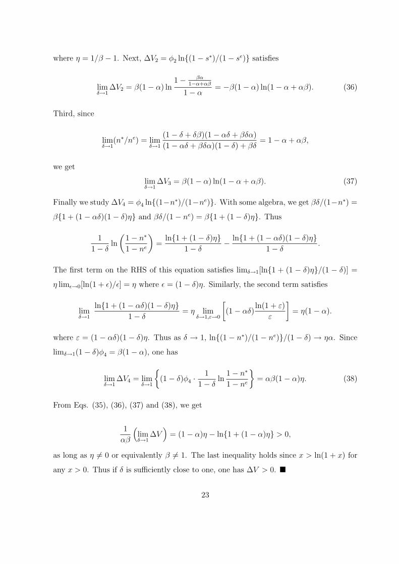
Finally we study ∆V4 = φ4 ln{(1−n∗)/(1−ne)}. With some algebra, we get βδ/(1−n∗) =

β{1 + (1 − αδ)(1 − δ)η} and βδ/(1 − ne) = β{1 + (1 − δ)η}. Thus

1

1 − δln

(1 − n∗

1 − ne

)=

ln{1 + (1 − δ)η}1 − δ

− ln{1 + (1 − αδ)(1 − δ)η}1 − δ

.

The first term on the RHS of this equation satisfies limδ→1[ln{1 + (1 − δ)η}/(1 − δ)] =

η limϵ→0[ln(1 + ϵ)/ϵ] = η where ϵ = (1 − δ)η. Similarly, the second term satisfies

limδ→1

ln{1 + (1 − αδ)(1 − δ)η}1 − δ

= η limδ→1,ε→0

[(1 − αδ)

ln(1 + ε)

ε

]= η(1 − α).

where ε = (1 − αδ)(1 − δ)η. Thus as δ → 1, ln{(1 − n∗)/(1 − ne)}/(1 − δ) → ηα. Since

limδ→1(1 − δ)φ4 = β(1 − α), one has

limδ→1

∆V4 = limδ→1

{(1 − δ)φ4 ·

1

1 − δln

1 − n∗

1 − ne

}= αβ(1 − α)η. (38)

From Eqs. (35), (36), (37) and (38), we get

1

αβ

(limδ→1

∆V)

= (1 − α)η − ln{1 + (1 − α)η} > 0,

as long as η = 0 or equivalently β = 1. The last inequality holds since x > ln(1 + x) for

any x > 0. Thus if δ is sufficiently close to one, one has ∆V > 0. ¥

23

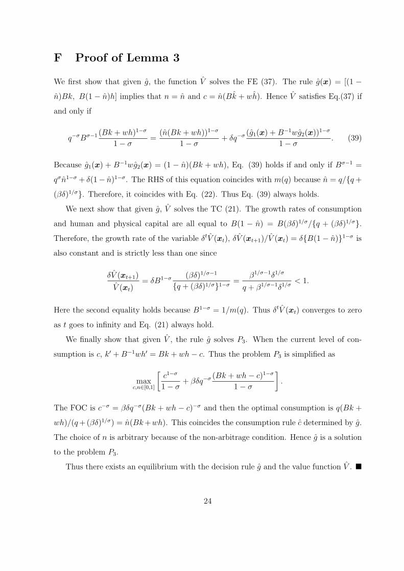
F Proof of Lemma 3

We first show that given g, the function V solves the FE (37). The rule g(x) = [(1 −n)Bk, B(1 − n)h] implies that n = n and c = n(Bk + wh). Hence V satisfies Eq.(37) if

and only if

q−σBσ−1 (Bk + wh)1−σ

1 − σ=

(n(Bk + wh))1−σ

1 − σ+ δq−σ (g1(x) + B−1wg2(x))1−σ

1 − σ. (39)

Because g1(x) + B−1wg2(x) = (1 − n)(Bk + wh), Eq. (39) holds if and only if Bσ−1 =

qσn1−σ + δ(1− n)1−σ. The RHS of this equation coincides with m(q) because n = q/{q +

(βδ)1/σ}. Therefore, it coincides with Eq. (22). Thus Eq. (39) always holds.

We next show that given g, V solves the TC (21). The growth rates of consumption

and human and physical capital are all equal to B(1 − n) = B(βδ)1/σ/{q + (βδ)1/σ}.Therefore, the growth rate of the variable δtV (xt), δV (xt+1)/V (xt) = δ{B(1 − n)}1−σ is

also constant and is strictly less than one since

δV (xt+1)

V (xt)= δB1−σ (βδ)1/σ−1

{q + (βδ)1/σ}1−σ=

β1/σ−1δ1/σ

q + β1/σ−1δ1/σ< 1.

Here the second equality holds because B1−σ = 1/m(q). Thus δtV (xt) converges to zero

as t goes to infinity and Eq. (21) always hold.

We finally show that given V , the rule g solves P3. When the current level of con-

sumption is c, k′ + B−1wh′ = Bk + wh − c. Thus the problem P3 is simplified as

maxc,n∈[0,1]

[c1−σ

1 − σ+ βδq−σ (Bk + wh − c)1−σ

1 − σ

].

The FOC is c−σ = βδq−σ(Bk + wh − c)−σ and then the optimal consumption is q(Bk +

wh)/(q +(βδ)1/σ) = n(Bk +wh). This coincides the consumption rule c determined by g.

The choice of n is arbitrary because of the non-arbitrage condition. Hence g is a solution

to the problem P3.

Thus there exists an equilibrium with the decision rule g and the value function V . ¥

24

G Proof of Lemma 4

One has

m′(q) =q + β1/σδ1/σ − (q + β1/σ−1δ1/σ)(1 − σ)

(q + β1/σδ1/σ)2−σ= σ

q − q∗

(q + β1/σδ1/σ)2−σ.

Suppose 1 − σ − β > 0. Then we have q∗ > 0, m′(q) < 0 if q < q∗, m′(q) > 0 if q > q∗

and m′(q∗) = 0. ¥

H Proof of Proposition 4

We first prove the existence of the equilibrium. First, when the law of motion for aggregate

state G(x) is given, human and physical capital growth rate (1− n)B and working time n

are constant. In addition, the wage rate and the real interest rate are constant. Moreover,

when the initial state variables satisfy Eq. (24), rt = r0 = αA(nh0/k0)α−1 = B. Next,

as Lemma 2 shows, when the wage rate is constant and the real interest rate r is equal

to B, the individual decision rule g(x, x) = g(x) and the value function V (x, x) = V (x)

solves the problem of the current self. Finally, the individual decision rule and the law of

motion for the aggregate state G are consistent.

We next show the equilibrium multiplicity. We have already shown that for any

q satisfying the above equation, we can construct a recursive competitive equilibrium.

Therefore, if 1 − σ > β and Eq. (23) holds, there are multiple equilibria. Moreover,

n = q/{q + (βδ)1/σ} is an increasing function of q and the equilibrium with higher q has

lower growth rate. ¥

25

References

[1] R. Barro, Ramsey meets Laibson in the neoclassical growth model, Quarterly Journal

of Economics 114 (1999), 1125-52.

[2] J. Benhabib, R. Perli, Uniqueness and indeterminacy: on the dynamics of endogenous

growth, Journal of Economic Theory 63 (1994), 113-142.

[3] U. Benzion, A. Rapaport, J. Yagil, Discount rates inferred from decisions: an exper-

imental study, Management Science 35 (1989), 270-284.

[4] D. Bethmann, A closed-form solution of the Uzawa-Lucas model of endogenous

growth, Journal of Economics 90 (2007), 87-107.

[5] M. Bils, P. Klenow, Does schooling cause growth?, American Economic Review 90

(2000), 1160-1183.

[6] E. Bond, P. Wang, C. Yip, A general two-sector model of endogenous growth with

human and physical capital: balanced growth and transitional dynamics, Journal of

Economic Theory 68 (1996), 149-173.

[7] J. Caballe, M. Santos, On endogenous growth with physical and human capital,

Journal of Political Economy 101 (1993), 1042-1067.

[8] A. Ciccone, E. Papaioannou, Human capital, the structure of production, and growth,

Review of Economics and Statistics 91 (2009), 66-82.

[9] D. Cohen, M. Soto, Growth and human capital: good data, good results, Journal of

Economic Growth 12 (2007), 51-76.

[10] O. Coibion, Y. Gorodnichenko, J. Wieland, The optimal inflation rate in New Key-

nesian models: should central banks raise their inflation targets in the light of the

ZLB?, (2011) mimeo.

[11] P. Diamond, B. Koszegi, Quasi-hyperbolic discounting and retirement, Journal of

Public Economics 87 (2003), 1839-1872.

26

[12] F. Garcıa-Belenguer, Stability, global dynamics and Markov equilibrium in models

of endogenous economic growth, Journal of Economic Theory 136 (2007), 392-416.

[13] P. Garcia-Castrillo, M. Sanso, Human capital and optimal policy in a Lucas-type

model, Review of Economic Dynamics 3 (2000), 757-70.

[14] M. Gomez, Optimal fiscal policy in Uzawa-Lucas model with externalities, Economic

Theory 22 (2002), 917-25.

[15] E. Henriksen, F. Kydland, Endogenous money, inflation and welfare, Review of Eco-

nomic Dynamics 13 (2010), 470-86.

[16] L. Jones, R. Manuelli, P. Rossi, Optimal taxation in models of endogenous growth,

Journal of Political Economy 101 (1993), 485-517.

[17] P. Krusell, B. Kuruscu, A. Smith, Equilibrium welfare and government policy with

quasi-geometric discounting, Journal of Economic Theory 105 (2002), 42-72.

[18] P. Krusell, T. Mukoyama, A. Sahin, A. Smith, Revisiting the welfare effects of elim-

inating business cycles, Review of Economic Dynamics 12 (2009), 393-404.

[19] P. Krusell, A. Smith, Consumption-savings decisions with quasi-geometric discount-

ing, Econometrica 71 (2003), 365-375.

[20] A. Ladron-de-Guevara, S. Ortigueira, M. Santos, A model of endogenous growth with

leisure, Review of Economic Studies 66 (1999), 609-632.

[21] D. Laibson, Golden eggs and hyperbolic discounting, The Quarterly Journal of Eco-

nomics, 112 (1997), 443-77.

[22] D. Laibson, Hyperbolic discounting functions, Undersaving and savings policy, Na-

tional Bureau of Economic Research Working Paper, No. 5635 (2001).

[23] R. Lucas, On the mechanics of economic development, Journal of Monetary Eco-

nomics 22 (1988), 3-42.

27

[24] L. Maliar, S. Maliar, Indeterminacy in a log-linearized neoclassical growth model

with quasi-geometric discounting, Economic Modelling 23 (2006), 492-505.

[25] G. Mankiw, D. Romer, D. Weil, A contribution to the empirics of economic growth,

Quarterly Journal of Economics 107 (1992), 407-437.

[26] E. Phelps, R. Pollak, On second-best national saving and game-equilibrium growth,

Review of Economic Studies 35 (1968), 185-199.

[27] R. Pollak, Consistent planning, Review of Economic Studies 35 (1968), 201-208.

[28] A. Rubinstein, Economics and psychology? The case of hyperbolic discounting, In-

ternational Economic Review 44 (2003), 1207-1216.

[29] M. Salois, C. Moss, A direct test of hyperbolic discounting using market asset data,

Economics Letters 112 (2011), 290-292.

[30] F. Salanie, N. Treich, Over-savings and hyperbolic discounting, European Economic

Review 50 (2006), 1557-1570.

[31] M. Schwarz, E. Sheshinski, Quasi-hyperbolic discounting and social security systems,

European Economic Review 51 (2007), 1247-1262.

[32] N. L. Stokey, R. E. Lucas, E. C. Prescott, Recursive methods in economic dynamics,

Harvard University Press, Cambridge, MA, 1989.

[33] R. Strotz, Myopia and inconsistency in dynamic utility maximization, Review of

Economic Studies 23 (1956), 165-180.

[34] R. Thaler, Some empirical evidence on dynamic inconsistency, Economic Letters 8

(1981), 201-207.

[35] H. Uzawa, Optimum technical change in an aggregative model of economic growth,

International Economic Review 6 (1965), 18-31.

28