on a quantum phase transition in a steady state out of ... a quantum phase transition in a steady...

On a quantum phase transition in a steady state outof equilibrium

Walter H. Aschbacher∗

Aix Marseille Universite, CNRS, CPT, UMR 7332, 13288 Marseille, FranceUniversite de Toulon, CNRS, CPT, UMR 7332, 83957 La Garde, France

Abstract

Within the rigorous axiomatic framework for the description of quantum mechanicalsystems with a large number of degrees of freedom, we show that the nonequilibriumsteady state, constructed in the quasifree fermionic system corresponding to the isotropicXY chain in which a finite sample, coupled to two thermal reservoirs at different tempera-tures, is exposed to a local external magnetic field, is breaking translation invariance andexhibits a strictly positive entropy production rate. Moreover, we prove that there existsa second-order nonequilibrium quantum phase transition with respect to the strength ofthe magnetic field as soon as the system is truly out of equilibrium.

Mathematics Subject Classifications (2010) 46L60, 47A40, 47B15, 82C10, 82C23.Keywords Open systems; nonequilibrium quantum statistical mechanics; quasifree fermions;Hilbert space scattering theory; nonequilibrium steady state; entropy production; nonequi-librium quantum phase transition.

1 Introduction

”As useful as the characterization of equilibrium states by thermostatic theory has proven tobe, it must be conceded that our primary interest is frequently in processes rather than instates. In biology, particularly, it is the life process that captures our imagination rather thanthe eventual equiilbrium [sic] state to which each organism inevitably proceeds.”

H. B. Callen [11, p.283]

A precise analysis of quantum mechanical systems having a large, i.e., often, in phys-ically idealized terms, an infinite number of degrees of freedom is most effectively carried

∗http://aschbacher.univ-tln.fr

1

2 Walter H. Aschbacher

out within the mathematically rigorous framework of operator algebras. As a matter of fact,having been heavily used in the 1960s for the description of quantum mechanical systems inthermal equilibrium, the benefits of this framework have again started to unfold more recentlyin the physically much more general situation of open quantum systems out of equilibrium.In the latter field, vast by its very nature, most of the mathematically rigorous results havebeen obtained for a particular family of states out of equilibrium, namely for the so-callednonequilibrium steady states (NESS) introduced in [17, p.6] as the large time limit of theaveraged trajectory of some initial state along the full time evolution. Beyond the challengingconstruction of this central object of interest in physically interesting situations, the deriva-tion, from first principles, of fundamental transport and quantum phase transition propertiesfor thermodynamically nontrivial systems out of equilibrium has also come within reach.

In both quantum statistical mechanics in and out of equilibrium, an important role isplayed by the so-called quasifree fermionic systems, and this is true not only with respect tothe mathematical accessibility but also when it comes to real physical applications. Namely,from a mathematical point of view, such systems allow for a simple and powerful descriptionby means of scattering theory restricted to the underlying one-particle Hilbert space overwhich the fermionic algebra of observables is constructed. This restriction of the dynamicsto the one-particle Hilbert space opens the way for a rigorous mathematical analysis ofmany properties which are of fundamental physical interest. On the other hand, they alsoconstitute a class of systems which are indeed realized in nature. One of the most prominentrepresentatives of this class is the so-called XY spin chain introduced in 1961 in [13, p.409]where a specific equivalence of this spin model with a quasifree fermionic system has beenestablished. Already in the 1960s, the first real physical candidate has been identified in [12,p.459] (see, for example, [15] for a survey of the rich interplay between the experimental andtheoretical research activity in the very dynamic field of low-dimensional magnetic systems).

In the present paper, we analyze transport and quantum phase transition properties forthe quasifree fermionic system over the two-sided discrete line corresponding, in the spinpicture, to the special case of the so-called isotropic XY spin chain. In order to model thedesired nonequilibrium situation as in [7, p.3431], we first fix

ν ∈ N0, (1)

and cut the finite piece of length 2ν + 1,

ZS := x ∈ Z | |x| ≤ ν, (2)

out of the two-sided discrete line. This piece plays the role of the configuration space of theconfined sample, whereas the remaining parts,

ZL := x ∈ Z |x ≤ −(ν + 1), (3)ZR := x ∈ Z |x ≥ ν + 1, (4)

act as the configuration spaces of the infinitely extended thermal reservoirs. Furthermore,over these configuration spaces, an initial decoupled state is prepared as the product of

On a quantum phase transition in a steady state out of equilibrium 3

three thermal equilibrium states carrying the corresponding inverse temperatures

0 = βS < βL < βR <∞. (5)

Finally, the NESS is constructed with respect to the full time evolution which not only recou-ples the sample and the reservoirs but also introduces a one-site magnetic field of strength

λ ∈ R (6)

at the origin.As a first result, we show that there exists a unique quasifree NESS, which we call the

magnetic NESS, whose translation invariance is broken as soon as the local magnetic fieldstrength λ is switched on. This property contrasts with the translation invariance of the NESSconstructed in [9, p.1158] for the anisotropic XY model with spatially constant magnetic field(see also Remark 3 below). Moreover, we explicitly determine the NESS expectation valueof the extensive energy current observable describing the energy flow through the samplefrom the left to the right reservoir. The form of this current immediately yields that the entropyproduction rate, the first fundamental physical quantity for systems out of equilibrium, isstrictly positive. Finally, we show that the system also exhibits what we call a second-ordernonequilibrium quantum phase transition, i.e., in the case at hand, a logarithmic divergenceof the second derivative of the entropy production rate with respect to the magnetic fieldstrength at the origin.

The present paper is organized as follows.Section 2 specifies the nonequilibrium setting, i.e., it introduces the observables, the quasifreedynamics, and the quasifree initial state.Section 3 contains the construction of the magnetic NESS and the proof of the breaking oftranslation invariance for nonvanishing magnetic field strength.Section 4 introduces the notions of energy current and entropy production rate. It also con-tains the determination of the heat flow and the strict positivity of the entropy production rate.Section 5 displays the last result, i.e., the proof of the existence of a second-order nonequi-librium quantum phase transition.Finally, the Appendix collects some ingredients used in the foregoing sections pertainingto the spectral theory of the magnetic Hamiltonian, the structure of the XY NESS, and theaction of the magnetic wave operators on completely localized wave functions.

2 Nonequilibrium setting

Remember that, in the operator algebraic approach to quantum statistical mechanics, aphysical system is specified by an algebra of observables, a group of time evolution au-tomorphisms, and a normalized positive linear state functional on this observable algebra(see, for example, the standard references [10] for more details).


In the Definition 1, 2, and 5 below, part (a) recalls the general formulation for quasifreefermionic systems and part (b) specializes to the concrete situation from [7, p.3431] whichwe are interested in in the present paper.

In the following, the commutator and the anticommutator of two elements a and b in thecorresponding sets in question read as usual as [a, b] := ab − ba and a, b := ab + ba,respectively.

Definition 1 (Observables)(a) Let h be the one-particle Hilbert space of the physical system. The observables are

described by the elements of the unital canonical anticommutation algebra A over hgenerated by the identity 1 and elements a(f) for all f ∈ h, where a(f) is antilinear in fand, for all f, g ∈ h, we have the canonical anticommutation relations

a(f), a(g) = 0, (7)a(f), a∗(g) = (f, g) 1, (8)

where (· , ·) denotes the scalar product of h.

(b) Let the configuration space of the physical system be given by the two-sided infinitediscrete line Z and let

h := `2(Z) (9)

be the one-particle Hilbert space over this configuration space.

The second ingredient is the time evolution. In order to define a quasifree dynamics, it issufficient, by definition, to specify its one-particle Hamiltonian, i.e., the generator of the timeevolution on the one-particle Hilbert space h. In general, a one-particle Hamiltonian is anunbounded selfadjoint operator on h (which is typically bounded from below though). Suchan action on the one-particle Hilbert space can be naturally lifted to the observable algebraA, becoming a group of automorphisms of A.

In the following, the set of (∗-)automorphisms of A will be written as Aut(A) and wedenote by L(h) and L0(h) the bounded operators and the finite rank operators on h, respec-tively. Moreover, for all r, q ∈ R, the Kronecker symbol is defined as usual by δrq := 1 if r = qand δrq := 0 if r 6= q. Furthermore, for all a ∈ L(h), we define the real part and the imaginarypart of a by Re(a) := (a + a∗)/2 and Im(a) := (a − a∗)/(2i), respectively. Finally, we seta0 := 1 ∈ L(h), and, if a is invertible, we use the notation a−n := (a−1)

n for all n ∈ N.

Definition 2 (Quasifree dynamics)(a) Let h be a Hamiltonian on h. The quasifree dynamics generated by h is the automor-

phism group defined, for all t ∈ R and all f ∈ h, by

τ t(a(f)) := a(eithf), (10)

and suitably extended to the whole of A.


(b) The right translation u ∈ L(h) and the localization projection p0 ∈ L0(h) are defined, forall f ∈ h and all x ∈ Z, by

(uf)(x) := f(x− 1), (11)p0f := f(0)δ0, (12)

where the elements of the usual completely localized orthonormal Kronecker basisδyy∈Z of h are given by δy(x) := δxy for all x ∈ Z. Moreover, let λ ∈ R denote themagnetic field strength and define the one-particle Hamiltonians h, hd, hλ ∈ L(h) by

h := Re(u), (13)hd := h− (vL + vR), (14)hλ := h+ λv, (15)

where the local external magnetic field v ∈ L0(h) and the decoupling operators vL, vR ∈L0(h) read

v := p0, (16)vL := Re(u−νp0u

ν+1), (17)vR := Re(uν+1p0u

−ν). (18)

The operators h, hd, and hλ will be called the XY Hamiltonian, the decoupled Hamil-tonian, and the magnetic Hamiltonian, respectively. The corresponding time evolutionautomorphisms of A are given by (10) and will be denoted by τ t, τ td, and τ tλ for all t ∈ R.

Remark 3 As mentioned in the Introduction, the model specified by Definition 1 and 2 hasits origin in the XY spin chain whose formal Hamiltonian reads

H = −1

4

∑x∈Z

(1 + γ)σ

(x)1 σ

(x+1)1 + (1− γ)σ

(x)2 σ

(x+1)2 + 2µσ

(x)3

, (19)

where γ ∈ (−1, 1) represents the anisotropy, µ ∈ R the spatially homogeneous magneticfield, and σ1, σ2, σ3 are the usual Pauli matrices. Indeed, using the so-called Araki-Jordan-Wigner transformation introduced in [5, p.279] (see also Remark 14), the Hamiltonian from(13) corresponds to the case of the so-called isotropic XY chain without magnetic field, i.e.,to the case with γ = µ = 0 in (19). In order to treat the anisotropic case γ 6= 0, one uses theso-called selfdual quasifree setting developed in [4, p.386]. In this most natural framework,one works in the doubled one-particle Hilbert space h ⊕ h and the generator of the trulyanisotropic XY dynamics has nontrivial off-diagonal blocks on h⊕ h (which vanish for γ = 0).In many respects, the truly anisotropic XY model is substantially more complicated than theisotropic one (this is true, a fortiori, if the magnetic field µ is switched on whose contributionto the generator acts diagonally on h⊕ h though).


Remark 4 For all α ∈ L, S,R, let us define the Hilbert space

hα := `2(Zα) (20)

over the sample and reservoir configuration spaces Zα defined in (2), (3), and (4), respec-tively. Moreover, for all α ∈ L, S,R, we define the map iα : hα → h, for all f ∈ hα and allx ∈ Z, by

(iαf)(x) :=

f(x), x ∈ Zα,0, x ∈ Z \ Zα,

(21)

and we note that its adjoint i∗α : h → hα is the operator acting by restriction to hα. With thehelp of these natural injections, we define the unitary operator w : h → hL ⊕ hS ⊕ hR, for allf ∈ h, by

wf := i∗Lf ⊕ i∗Sf ⊕ i∗Rf, (22)

and we observe that its inverse w−1 : hL ⊕ hS ⊕ hR → h is given by w−1(fL ⊕ fS ⊕ fR) =iLfL + iSfS + iRfR for all fL ⊕ fS ⊕ fR ∈ hL ⊕ hS ⊕ hR. Then, using (22), we can write

wvLw−1 =

1

2

0 (i∗Sδ−ν , · )i∗Lδ−(ν+1) 0(i∗Lδ−(ν+1), · )i∗Sδ−ν 0 0

0 0 0

, (23)

wvRw−1 =

1

2

0 0 00 0 (i∗Rδν+1, · )i∗Sδν0 (i∗Sδν , · )i∗Rδν+1 0

, (24)

where we used the same notation for the scalar products on hL, hS, and hR and for the oneon h. Computing whw−1 and using (23) and (24), we find that the decoupling operators vLand vR indeed decouple the sample from the reservoirs in the sense that

whdw−1 = hL ⊕ hS ⊕ hR, (25)

where, for all α ∈ L, S,R, the Hamiltonians hα ∈ L(hα) are defined by

hα := i∗αhiα. (26)

The last ingredient are the states, i.e., the normalized positive linear functionals on theobservable algebra A. As discussed in the Introduction, we are interested in quasifree states,i.e., in states whose many-point correlation functions factorize in determinantal form.

In the following, EA stands for the set of states on A. Moreover, for all n ∈ N, the n × nmatrix with entries aij ∈ C for all i, j ∈ 1, . . . , n is denoted by [aij]

ni,j=1.


Definition 5 (Quasifree states)

(a) Let s ∈ L(h) be an operator satisfying 0 ≤ s ≤ 1. A state ωs ∈ EA is called a quasifreestate induced by s if, for all n,m ∈ N, all f1, . . . , fn ∈ h, and all g1, . . . , gm ∈ h, we have

ωs(a∗(fn) . . . a∗(f1)a(g1) . . . a(gm)) = δnm det([(gi, sfj)]

ni,j=1). (27)

The operator s is called the two-point operator of the quasifree state ωs.

(b) The decoupled initial state is defined to be the quasifree state ωd ∈ EA induced by thetwo-point operator sd ∈ L(h) of the form

sd := ρ(βLiLhLi∗L + βRiRhRi

∗R), (28)

where, for all r ∈ R, the Planck density function ρr : R→ R is defined, for all e ∈ R, by

ρr(e) :=1

1 + ere, (29)

and, in (28), we used the simplified notation ρ := ρ1.

Remark 6 In the selfdual quasifree setting mentioned in Remark 3, the quasifreeness of astate is expressed by means of a pfaffian of the two-point correlation matrix with respect tothe generators of the selfdual canonical anticommutation algebra (see, for example, [7, p.3447]).

Remark 7 Using the unitarity of w ∈ L(h, hL ⊕ hS ⊕ hR) from (22), the unitary invariance ofthe spectrum, the uniqueness of the continuous functional calculus, and

wiLhLi∗Lw−1 = hL ⊕ 0⊕ 0, (30)

wiRhRi∗Rw−1 = 0⊕ 0⊕ hR, (31)

the two-point operator of the decoupled quasifree initial state can be written as

wsdw−1 = wρ(βLiLhLi

∗L + βRiRhRi

∗R)w−1

= ρ(w(βLiLhLi∗L + βRiRhRi

∗R)w−1)

= ρ(βLhL ⊕ 0⊕ βRhR)

= ρβL(hL)⊕ 121⊕ ρβR(hR), (32)

i.e., the two-point operator sd does not couple the sample and the reservoir subsystems asrequired by our nonequilibrium setting.

One of the main motivations for introducing the magnetic Hamiltonian (15) in [7, p.3432]was to study the effect of the breaking of translation invariance. For quasifree states as givenin Definition 5 (a), this property can be defined as follows.


Definition 8 (Translation invariance) A quasifree state ωs ∈ EA induced by the two-pointoperator s ∈ L(h) is called translation invariant if

[s, u] = 0, (33)

where u ∈ L(h) is the right translation from (11).

Remark 9 By using the translation automorphism τu ∈ Aut(A) defined by τu(a(f)) := a(uf)for all f ∈ h and suitably extended to the whole of A, we note that a quasifree state ωs ∈ EA

is translation invariant if and only if ωs τu = ωs.

3 Nonequilibrium steady state

The definition of a nonequilibrium steady state (NESS) below stems from [17, p.6]. Weimmediately specialize it to the case at hand.

In the following, if nothing else is explicitly stated, we will always use the assumptions0 = βS < βL < βR <∞ and λ ∈ R from (5) and (6). Moreover, we will also use the notation

δ :=βR − βL

2, (34)

β :=βR + βL

2. (35)

Definition 10 (Magnetic NESS) The state ωλ ∈ EA, defined, for all A ∈ A, by

ωλ(A) := limt→∞

ωd(τ tλ(A)), (36)

is called the magnetic NESS associated with the decoupled quasifree initial state ωd ∈ EA

and the magnetic dynamics τ tλ ∈ Aut(A) for all t ∈ R.

Remark 11 The more general definition in [17, p.6] defines a NESS as a weak-∗ limit pointfor T →∞ of

1

T

∫ T

0

dt ωd τ tλ. (37)

This averaging procedure implies, in general, the existence of a limit point. In particular, inthe quasifree setting, it allows to treat a nonvanishing contribution to the point spectrum ofthe one-particle Hamiltonian generating the full time evolution. In the present case, since,due to Proposition 31 (c) from Appendix A, the Hamiltonian hλ has a single eigenvalue, (36)is sufficient to extract a limit from the point spectrum subspace (see (49) below).


In [7, p.3436], we found that the magnetic NESS is a quasifree state induced by a two-point operator sλ ∈ L(h) whose form could be determined with the help of scattering the-ory on the one-particle Hilbert space h. In particular, we made use of the wave operatorw(hd, hλ) ∈ L(h) defined by

w(hd, hλ) := s− limt→∞

e−ithdeithλ1ac(hλ), (38)

where 1ac(hλ) ∈ L(h) denotes the spectral projection onto the absolutely continuous sub-space of the magnetic Hamiltonian hλ. Moreover, we will also need the spectral projection1pp(hλ) ∈ L(h) onto the pure point subspace of hλ. All the spectral properties of the magneticHamiltonian hλ which we will use in the following are summarized in Appendix A.

Theorem 12 (Magnetic two-point operator) The magnetic NESS ωλ is the quasifree stateinduced by the two-point operator sλ ∈ L(h) given by

sλ = w∗(hd, hλ)sdw(hd, hλ) + 1pp(hλ)sd1pp(hλ). (39)

Moreover, if λ 6= 0, the pure point subspace of hλ ∈ L(h) is one-dimensional.

Remark 13 For all γ ∈ (−1, 1) and all µ ∈ R in (19), the so-called XY NESS has been con-structed in [9, p.1170] using time dependent scattering theory (see Theorem 32 of AppendixB for the XY NESS with γ = µ = 0). The two-point operator of the XY NESS for γ = µ = 0coincides with the two-point operator of the magnetic NESS for λ = 0.

Remark 14 For the special case γ = µ = 0, the XY NESS has also been found in [6] withthe help of asymptotic approximation methods. The construction of the XY NESS in [6]and [9] is carried out within the mathematically rigorous axiomatic framework of operatoralgebras for the description of quantum mechanical systems having an infinite number ofdegrees of freedom. Due to the two-sidedness of the present nonequilibrium setting, thepassage from the spin algebra to the canonical anticommutation algebra relies on the so-called Araki-Jordan-Wigner transformation introduced in [5, p.279]. In contrast to the caseof the usual Jordan-Wigner transformation for finite or infinite one-sided systems, the directcorrespondence between these two algebras breaks down in the thermodynamic limit of aninfinite chain which extends in both directions.

Remark 15 In [9, p.1158], we observed that the XY NESS can be written, formally, as anequilibrium state specified by the inverse temperature β and an effective Hamiltonian whichdiffers from the original XY Hamiltonian by conserved long-range multi-body charges (in [14,p.914], it has been proved though that, if βL 6= βR, there exists no strongly continuous one-parameter automorphism group of the spin algebra with respect to which the XY NESS isan equilibrium [KMS] state). The Lagrange multiplier approach of [3, p.168] (see also [2,p.5186]), set up for a chain of finite length, directly defines a NESS as the ground stateof an effective Hamiltonian which differs from the original Hamiltonian by the conservedmacroscopic energy current observable. As formally discussed in [16, p.168], the effectiveHamiltonian constructed in this way is substantially different from the one corresponding to


the XY NESS in that it only contains a finite subfamily of the infinite family of all the chargespresent in the latter situation. Moreover, since the XY NESS consists of left movers andright movers carrying the inverse temperatures βR and βL of the right and left reservoirs,respectively (cf. [9, p.1171]), the exponential decay of the transversal spin-spin correlationfunction (cf. [8, p.10]) contrasts with its weak power law behavior in the Lagrange multiplierapproach.

For the sake of completeness, we display the proof of Theorem 12 given in [7, p.3437].

Proof. Since A is generated by the identity 1 and the elements a(f) for all f ∈ h, since|ωd(τ tλ(A))| ≤ ‖A‖ for all t ∈ R and all A ∈ A, and since ωd satisfies the determinantalfactorization property (27), it is enough to study, for all n ∈ N, the large time limit of

ωd(τ tλ(a∗(fn) . . . a∗(f1)a(g1) . . . a(gn))) = det(Ω(t)), (40)

where the map Ω : R→ Mat(n,C) is defined, for all t ∈ R and all i, j ∈ 1, . . . , n, by

Ωij(t) := (eithλgi, sdeithλfj), (41)

and Mat(n,C) stands for the set of complex n× n matrices. Moreover, since, due to Propo-sition 31 (a) from Appendix A, the singular continuous spectrum of hλ is empty, we have1 = 1ac(hλ) + 1pp(hλ). Thus, inserting 1 between the propagator and the wave function onboth sides of the scalar product in (41), we can write, for all t ∈ R and all i, j ∈ 1, . . . , n,that

Ωij(t) = Ωaaij (t) + Ωap

ij (t) + Ωpaij (t) + Ωpp

ij (t), (42)

where the maps Ωaa,Ωap,Ωpa,Ωpp : R → Mat(n,C) are defined, for all t ∈ R and all i, j ∈1, . . . , n, by

Ωaaij (t) := (eithλ1ac(hλ)gi, sdeithλ1ac(hλ)fj), (43)

Ωapij (t) := (eithλ1ac(hλ)gi, sdeithλ1pp(hλ)fj), (44)

Ωpaij (t) := (eithλ1pp(hλ)gi, sdeithλ1ac(hλ)fj), (45)

Ωppij (t) := (eithλ1pp(hλ)gi, sdeithλ1pp(hλ)fj). (46)

Term Ωaaij

Using that [hd, sd] = 0 which follows from (25) and (32), the large time limit of (43) yields thewave operator contribution to sλ in (39) since, for all i, j ∈ 1, . . . , n, we have

limt→∞

Ωaaij (t) = lim

t→∞(e−ithdeithλ1ac(hλ)gi, sde−ithdeithλ1ac(hλ)fj)

= (gi, w∗(hd, hλ)sdw(hd, hλ)fj). (47)

Terms Ωapij and Ωpa

ij

The large time limit of (44) behaves, for all i, j ∈ 1, . . . , n, like

limt→∞|Ωap

ij (t)| ≤ limt→∞‖1pp(hλ)sdeithλ1ac(hλ)gi‖‖fj‖

= 0, (48)


where we used the Riemann-Lebesgue lemma and the fact from Proposition 31 (c) of Ap-pendix A that 1pp(hλ) ∈ L0(h). The estimate from (48) also holds true for the term (45), ofcourse.

Term Ωppij

Since, if λ 6= 0, the subspace ran (1pp(hλ)) is spanned by the normalized eigenfunctionfλ ∈ h corresponding to the eigenvalue eλ given in Proposition 31 (c) of Appendix A, wehave eithλ1pp(hλ) = eiteλ1pp(hλ) for all t ∈ R. This implies, for all t ∈ R and all i, j ∈ 1, . . . , n,that (46) reads as

Ωppij (t) := (gi, 1pp(hλ)sd1pp(hλ)fj). (49)

Finally, since the map det : Mat(n,C)→ C is continuous, we arrive at the conclusion.

We next show that, as soon as the magnetic field strength is nonvanishing, the magneticNESS breaks translation invariance. In order to do so, we switch to momentum space

h := L2([−π, π]; dk2π

) (50)

by means of the unitary Fourier transform f : h → h which is defined, as usual, by ff :=∑x∈Z f(x)ex for all f ∈ h, and for all x ∈ Z, the plane wave function ex : [−π, π]→ C is given

by ex(k) := eikx for all k ∈ [−π, π].

In the following, we will also use the notation a := faf∗ ∈ L(h) for all a ∈ L(h). Hence,in momentum space, the XY Hamiltonian h acts through multiplication by the dispersionrelation function ε : [−π, π]→ R defined, for all k ∈ [−π, π], by

ε(k) := cos(k). (51)

The function introduced next will capture the effect of a nonvanishing strength of the localexternal magnetic field. Its action will also be particularly visible in the description of the heatflux in Theorem 24 below.

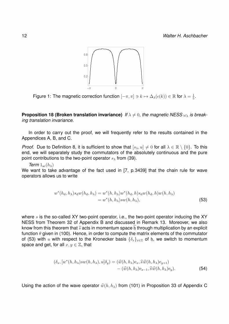
Definition 16 (Magnetic correction function) The function ∆λ : [−1, 1] → R, defined, forall e ∈ [−1, 1], by

∆λ(e) :=

1−e2

1−e2+λ2 , λ 6= 0,

1, λ = 0,(52)

is called the magnetic correction function (see Figure 1).

Remark 17 The magnetic correction function also plays an important role in the mechanismwhich regularizes the symbol of the Toeplitz operator describing a certain class of nonequi-librium correlation functions in the magnetic NESS (see [7, p.3441]).


-π 0 π

0.2

0.5

0.8

Figure 1: The magnetic correction function [−π, π] 3 k 7→ ∆λ(ε(k)) ∈ R for λ = 15.

Proposition 18 (Broken translation invariance) If λ 6= 0, the magnetic NESS ωλ is break-ing translation invariance.

In order to carry out the proof, we will frequently refer to the results contained in theAppendices A, B, and C.

Proof. Due to Definition 8, it is sufficient to show that [sλ, u] 6= 0 for all λ ∈ R \ 0. To thisend, we will separately study the commutators of the absolutely continuous and the purepoint contributions to the two-point operator sλ from (39).

Term 1ac(hλ)We want to take advantage of the fact used in [7, p.3439] that the chain rule for waveoperators allows us to write

w∗(hd, hλ)sdw(hd, hλ) = w∗(h, hλ)w∗(hd, h)sdw(hd, h)w(h, hλ)

= w∗(h, hλ)sw(h, hλ), (53)

where s is the so-called XY two-point operator, i.e., the two-point operator inducing the XYNESS from Theorem 32 of Appendix B and discussed in Remark 13. Moreover, we alsoknow from this theorem that s acts in momentum space h through multiplication by an explicitfunction θ given in (100). Hence, in order to compute the matrix elements of the commutatorof (53) with u with respect to the Kronecker basis δxx∈Z of h, we switch to momentumspace and get, for all x, y ∈ Z, that

(δx, [w∗(h, hλ)sw(h, hλ), u]δy) = (w(h, hλ)ex, s w(h, hλ)ey+1)

− (w(h, hλ)ex−1, s w(h, hλ)ey). (54)

Using the action of the wave operator w(h, hλ) from (101) in Proposition 33 of Appendix C


on the plane wave functions ex = fδx for all x ∈ Z, we find, for all x, y ∈ Z, that

(w(h, hλ)ex, s w(h, hλ)ey) =

∫ π

−π

dk

2πθ(k) eik(y−x)

+ iλ

∫ π

−π

dk

2πθ(k)

sin(|k|)sin2(k) + λ2

(ei(|ky|−kx) − ei(ky−|kx|)

)− λ2

∫ π

−π

dk

2π

θ(k)

sin2(k) + λ2(ei(|ky|−kx) + ei(ky−|kx|) − ei|k|(|y|−|x|)

).

(55)

We next plug x = 0 and y = 1 into (54). Separating the positive and negative momentumcontributions in (55), regrouping with respect to the temperature dependence of θ, and re-assembling the terms over the whole momentum interval with the help of the evenness of εfrom (51), we find, for all λ ∈ R \ 0, that

(δ0, [w∗(h, hλ)sw(h, hλ), u]δ1) = iλ

∫ π

−π

dk

2πθ(k)


(e2i|k| − e2ik

)− λ2

∫ π

−π

dk

2π

θ(k)

sin2(k) + λ2e2ik

− iλ

∫ π

−π

dk

2πθ(k)


(ei(|k|+k) − ei(k−|k|)

)+ λ2

∫ π

−π

dk

2π

θ(k)

sin2(k) + λ2(ei(|k|+k) + ei(k−|k|) − 1

)= λ

∫ π

−π

dk

2πε(k)[ρβL(ε(k))− ρβR(ε(k))] ∆λ(ε(k)). (56)

Term 1pp(hλ)Due to Proposition 31 (c) of Appendix A, we know that the pure point subspace of themagnetic Hamiltonian is spanned by the exponentially localized eigenfunction fλ ∈ h givenin (99). Hence, for all x, y ∈ Z, we can write

(δx, [1pp(hλ)sd1pp(hλ), u]δy) = (fλ, sdfλ)[fλ(x)fλ(y + 1)− fλ(x− 1)fλ(y)]. (57)

Plugging x = 0 and y = 1 into (57) and using the form of fλ from (99), we get that

(δ0, [1pp(hλ)sd1pp(hλ), u]δ1) = 0. (58)

Hence, with the help of (56), (52), and (58), we arrive at the conclusion.

Remark 19 Since 1/(1 + ex)− 1/(1 + ey) = sinh[(y−x)/2]/(cosh[(y−x)/2] + cosh[(y+x)/2)])for all x, y ∈ R, the difference of the Planck density functions in (56) reads, for all x ∈ R, as

ρβL(x)− ρβR(x) =sinh(δx)

cosh(δx) + cosh(βx), (59)

where we used the definitions (34) and (35).


4 Entropy production

One of the central physical notions for systems out of equilibrium is the well-known entropyproduction rate being a bilinear form in the affinities, driving the system out of equilibrium,and in the fluxes, describing the response to these applied forces. In the present situation,these quantities correspond to the differences between the inverse temperature of eachreservoir and the inverse temperature of the sample and to the corresponding heat fluxes(see, for example, [17, p.8] and [9, p.1159], and references therein). Hence, we are led tothe following definition.

Definition 20 (Energy current observable) Let α ∈ L,R. The one-particle energy cur-rent observable ϕα ∈ L(h), describing the energy flow from reservoir α into the sample, isdefined by

ϕα := − d

dt

∣∣∣∣t=0

eithλiαhαi∗αe−ithλ . (60)

Moreover, the extensive energy current observable Φα := dΓ(ϕα) is the usual second quan-tization of ϕα.

The entropy production rate then reads as follows.

Definition 21 (Entropy production rate) The entropy production rate in the magnetic NESSωλ is defined by

σλ := −∑

α∈L,R

βαJλ,α, (61)

where the NESS expectation value of the extensive energy current observable, the so-calledheat flux, has been denoted, for all α ∈ L,R, by

Jλ,α := ωλ(Φα). (62)

Remark 22 Since, for all α ∈ L,R, we have ϕα = −i[hλ, iαhαi∗α] = −i[h, iαhαi

∗α], we see

that ϕα is independent of λ and that

ϕL =1

2Im(u−νp0u

ν+2), (63)

ϕR =1

2Im(uνp0u

−(ν+2)), (64)

i.e., ϕα ∈ L0(h) which implies that Φα ∈ A(h) (the latter statement also holds in the moregeneral case of trace class operators in the selfdual setting, see [4, p.410, 412]). Hence, σλis well-defined.


Remark 23 Using that∑

α∈L,R iαhαi∗α = h− iShSi∗S − (vL + vR), we can write∑

α∈L,R

ϕα = i[hλ, q], (65)

where we set q := iShSi∗S + vL + vR + λv. Hence, since q ∈ L0(h), we can write∑

α∈L,R

Φα = dΓ(i[hλ, q])

=d

dt

∣∣∣∣t=0

τ tλ(dΓ(q)). (66)

Taking the NESS expectation value of (66) and using that, due to (36), ωλ is τ tλ-invariant forall t ∈ R, we find the first law of thermodynamics, i.e.,∑

α∈L,R

Jλ,α = 0. (67)

Due to (61) and (67), we restrict ourselves to the study of the NESS expectation valueof the extensive energy current describing the energy flow from the left reservoir into thesample, and we will use the simplified notation Jλ := Jλ,L in the following.

Theorem 24 (Heat flux) The heat flux, i.e., the NESS expectation value of the extensiveenergy current observable describing the energy flow from the left reservoir into the samplehas the form

Jλ =1

2

∫ π

−π

dk

2πj(ε(k)) ∆λ(ε(k)), (68)

where the density function j : [−1, 1]→ R is defined, for all e ∈ [−1, 1], by

j(e) := e√

1− e2[ρβL(e)− ρβR(e)

], (69)

and the functions ρβL , ρβR , ε, and ∆λ are given in (29), (51), and (52), respectively (seeFigure 2).

Remark 25 Since, due to the proof of Theorem 28 (a) below, we have that (j∆λ) ε ∈L1([−π, π]; dk), the integral (68) is well-defined.

Remark 26 Note that (68) is independent of the sample size parameter ν.

Proof. The case λ = 0 is treated in [9, p.1160] (see Remark 3 above) and corresponds tothe triviality of the magnetic correction function ∆0 = 1 in (68).

In the following, we thus discuss the case λ 6= 0. Using (39) and the fact that ωλ(dΓ(ϕ)) =tr(sλϕ) for all ϕ ∈ L0(h) (a similar statement also holds in the more general case of trace


-1 0 1

0.01

0.02

0.03

Figure 2: The heat flux R 3 λ 7→ Jλ ∈ R as a function of the strength of the local externalmagnetic field for βL = 1 and βR = 2.

class operators in the selfdual setting, see [4, p.410, 412]), the NESS expectation value ofthe extensive energy current observable describing the energy flow from the left reservoirinto the sample can be written in the form

Jλ = ωλ(ΦL)

= ωλ(dΓ(ϕL))

= tr(sλϕL)

= Jλ,ac + Jλ,pp, (70)

where we make the definitions

Jλ,ac := tr(w∗(hd, hλ)sdw(hd, hλ)ϕL), (71)Jλ,pp := tr(1pp(hλ)sd1pp(hλ)ϕL). (72)

We next discuss the two terms (71) and (72) separately.Term Jλ,ac

Using (53), (63), the Kronecker basis δxx∈Z of h and the fact that the two-point operator sis selfadjoint, we can write

Jλ,ac =1

2tr(w∗(h, hλ)sw(h, hλ)Im(u−νp0u

ν+2))

=1

2Im[(w(h, hλ)δ−(ν+2), sw(h, hλ)δ−ν)]. (73)

In order to compute (73), we proceed as in the proof of Proposition 18 and switch to mo-mentum space h. Using (55) for x = −(ν + 2) and y = −ν, we then get

(w(h, hλ)e−(ν+2), s w(h, hλ)e−ν) =3∑i=1

zi, (74)


where we make the definitions

z1 :=

∫ π

−π

dk

2πθ(k) e2ik (75)

z2 := iλ

∫ π

−π

dk

2πθ(k)


(ei(|k|ν+k(ν+2)) − e−i(kν+|k|(ν+2))

)(76)

z3 := −λ2∫ π

−π

dk

2π

θ(k)

sin2(k) + λ2(ei(|k|ν+k(ν+2)) + e−i(kν+|k|(ν+2)) − e−2i|k|

), (77)

and we recall that θ is given in (100) of Theorem 32 in Appendix B. Separating the positiveand negative momentum contributions (which directly leads to (79)), regrouping with respectto the temperature dependence of θ, and reassembling the terms over the whole momentuminterval with the help of the evenness of ε, the imaginary parts take the form

Im(z1) =

∫ π

−π

dk

2πcos(k)| sin(k)|[ρβL(cos(k))− ρβR(cos(k))], (78)

Im(z2) = 0, (79)

Im(z3) = −λ2∫ π

−π

dk

2πcos(k)| sin(k)|[ρβL(cos(k))− ρβR(cos(k))]

1

sin2(k) + λ2. (80)

Therefore, (78), (79), and (80) lead us to

Jλ,ac =1

2

∫ π

−π

dk


sin2(k)

sin2(k) + λ2. (81)

Term Jλ,ppSince the one-particle energy current observable ϕL = −i[hλ, iLhLi

∗L] has the form of a

commutator, the cyclicity of the trace implies that

Jλ,pp = tr(sd1pp(hλ)ϕL1pp(hλ))

= −i tr(sd1pp(hλ)[hλ, iLhLi∗L]1pp(hλ))

= −i tr(sd1pp(hλ)[eλ1, iLhLi∗L]1pp(hλ))

= 0, (82)

where eλ is the unique eigenvalue of the magnetic Hamiltonian hλ given in Proposition 31 (c)of Appendix A.

Hence, using (81), (82), (52), and (69), we arrive at the conclusion.

Corollary 27 (Strict positivity of the entropy production) The heat flux is flowing throughthe sample from the hotter to the colder reservoir. Moreover, the entropy production rate isstrictly positive,

σλ > 0. (83)


Proof. It immediately follows from (68) and the form of the functions (52) and (69) thatJλ > 0. Moreover, using (61) and (67), the entropy production can be written as

σλ = (βR − βL)Jλ. (84)

Hence, we arrive at the conclusion.

5 Nonequilibrium quantum phase transition

Going beyond Ehrenfest’s classification proposition not only with respect to the nature of thesingularity, as it is usually done in the modern classification schemes, but also with respectto the nature of the state considered, we define a nonequilibrium quantum phase transitionto be a point of (higher-order) non-differentiability of the entropy production rate with respectto an external physical parameter of interest. In the case at hand, the parameter which weare interested in is the local external magnetic field λ.

In the following, J ′λ will denote the derivative of Jλ with respect to λ.

Theorem 28 (Second-order nonequilibrium quantum phase transition) The heat flux R 3λ 7→ Jλ ∈ R has the following properties:

(a) It belongs to C1(R) ∩ C∞(R \ 0).

(b) Its second derivative with respect to the local external magnetic field does not exist atthe origin, i.e., for λ→ 0, we have

J ′λ = Cλ log(|λ|) +O(λ), (85)

where we set C := (4/π)[ρ(βL)− ρ(βR)].

Remark 29 In [1, p.4], an interesting study of a class of nonequilibrium quantum phasetransitions in the NESS constructed in [9, p.1158] has been carried out. In particular, it hasbeen shown that current type correlation functions in this NESS have a discontinuous firstand third derivative with respect to the spatially homogeneous external magnetic field µ (atdifferent (γ, µ)-values on the so-called nonequilibrium critical line) as soon as the anisotropyγ is nonvanishing (cf. Remark 3).

Remark 30 In the Lagrange multiplier approach discussed in Remark 15, the expectationvalue of the macroscopic energy current observable in the ground state of the effectiveHamiltonian defines a phase diagram in the effective field-magnetic field plane (cf. [3, p.169]) separating the equilibrium phase, in which the heat flux is zero, from the nonequi-librium phase of nonvanishing heat flux (in the latter phase, the spin-spin correlations in


the x direction also exhibit an oscillatory behavior dominated by a slowly decaying ampli-tude). This interpretation contrasts with Theorem 28 which yields a point of second-ordernon-differentiability of the always strictly positive entropy production rate.

Proof. We start off by noting that the function f : R× [−π, π]→ R, defined, for all λ ∈ R andall k ∈ [−π, π], by

f(λ, k) := j(ε(k)) ∆λ(ε(k))

= j(cos(k)) ·

sin2(k)

sin2(k)+λ2, λ 6= 0,

1, λ = 0,(86)

is integrable in k over [−π, π] for any fixed λ ∈ R since |j(cos(k))| ≤ 2 for all k ∈ [−π, π] andsince sin2(k)/(sin2(k) + λ2) ≤ 1 for all λ 6= 0 and all k ∈ [−π, π].

Using Lebesgue’s dominated convergence theorem, we can now proceed to study theregularity of the heat flux.

(a) J· ∈ C(R)We first want to show that f( · , k) ∈ C(R) for any fixed k ∈ [−π, π]. In order to do so, wenote that, since j(cos(k)) = 0 and ∆λ(cos(k)) = δ0λ for all k ∈ 0,±π and all λ ∈ R, weget that f( · , k) = 0 for all k ∈ 0,±π, i.e., f( · , k) ∈ C(R) for all k ∈ 0,±π. Moreover,(86) immediately implies that f( · , k) ∈ C(R) for all k ∈ [−π, π]\0,±π. Second, sincewe have from above that |f(λ, k)| ≤ 2 ∈ L1([−π, π]; dk) for all λ ∈ R and all k ∈ [−π, π],Lebesgue’s dominated convergence theorem implies that J· ∈ C(R).

J· ∈ C1(R)Again, first, we immediately get that f( · , k) ∈ C1(R) for all k ∈ 0,±π and f( · , k) ∈C1(R \ 0) for all k ∈ [−π, π] \ 0,±π. Moreover, for any fixed k ∈ [−π, π] \ 0,±π,we have limλ→0(f(λ, k)− f(0, k))/λ = 0. Therefore, for all k ∈ [−π, π] \ 0,±π and allλ ∈ R, we get

∂f

∂λ(λ, k) = −2λj(cos(k))

sin2(k)

(sin2(k) + λ2)2, (87)

which implies that f( · , k) ∈ C1(R) for all k ∈ [−π, π] \ 0,±π. Second, since 0 ≤(| sin(k)| − |λ|)2 = sin2(k) − 2|λ|| sin(k)| + λ2 for all λ ∈ R and all k ∈ [−π, π], we canwrite 2|λ|| sin(k)|3 ≤ (sin2(k) + λ2)2 for all λ ∈ R and all k ∈ [−π, π]. Hence, since|j(cos(k))| ≤ 2| cos(k)|| sin(k)| for all k ∈ [−π, π], it follows, for all k ∈ [−π, π] \ 0,±πand all λ ∈ R, that ∣∣∣∣∂f∂λ(λ, k)

∣∣∣∣ ≤ 2 |cos(k)| 2|λ|| sin(k)|3

(sin2(k) + λ2)2, (88)

which leads to |∂f∂λ

(λ, k)| ≤ 2 ∈ L1([−π, π]; dk) for all λ ∈ R and all k ∈ [−π, π]. Hence,Lebesgue’s dominated convergence theorem implies that J· ∈ C1(R).


-1 0 1

-0.02

0

0.02

Figure 3: The first derivative of the heat flux with respect to the strength of the local externalmagnetic field R 3 λ 7→ J ′λ ∈ R for βL = 1 and βR = 2.

J· ∈ C∞(R \ 0)Since (86) tells us that, for all k ∈ [−π, π], the derivatives of any order of f( · , k) withrespect to λ exist and are bounded by a constant for all k ∈ [−π, π] and all points ina sufficiently small neighborhood of any λ 6= 0, Lebesgue’s dominated convergencetheorem also yields that J· ∈ C∞(R \ 0).

(b) Using (a), (87), (69), and (59), we get, for all λ ∈ R, that

J ′λ = −2λ

∫ π

−π

dk


sin2(k)

(sin2(k) + λ2)2

= −8λ

∫ π2

0

dk

2π

cos(k) sinh(δ cos(k))

cosh(δ cos(k)) + cosh(β cos(k))

sin3(k)

(sin2(k) + λ2)2, (89)

where, in the second equality, we reduced the integration interval from [−π, π] to [0, π]and then from [0, π] to [0, π/2] by using the coordinate transformations k 7→ −k andk 7→ π − k, respectively (see Figure 3). Next, using the coordinate transformationarcsin : [0, 1]→ [0, π

2] in (89), we can write, for all λ ∈ R \ 0, that (see Figure 4)

−π4

J ′λλ

=

∫ 1

0

dx f(x)x3

(x2 + λ2)2, (90)

where the function f : [0, 1]→ R is defined, for all x ∈ [0, 1], by

f(x) :=sinh(δ

√1− x2)

cosh(δ√

1− x2) + cosh(β√

1− x2). (91)

In order to extract the logarithmic divergence at the origin, we make the decomposition∫ 1

0

dx f(x)x3

(x2 + λ2)2= F1(λ) + F2(λ), (92)


-1 0 1

0

Figure 4: The second derivative of the heat flux with respect to the strength of the localexternal magnetic field R \ 0 3 λ 7→ J ′′λ ∈ R for βL = 1 and βR = 2.

where the functions F1, F2 : R \ 0 → R are defined, for all λ ∈ R \ 0, by

F1(λ) := f(0)

∫ 1

0

dxx3

(x2 + λ2)2, (93)

F2(λ) :=

∫ 1

0

dx [f(x)− f(0)]x3

(x2 + λ2)2. (94)

Term F1(λ)Using the primitive of its integrand, the first integral reads, for all λ ∈ R \ 0, as

F1(λ) = − sinh(δ)

cosh(δ) + cosh(β)log(|λ|)

− 1

2

sinh(δ)

cosh(δ) + cosh(β)

(1

1 + λ2− log(1 + λ2)

), (95)

and the second term on the right hand side of (95) is obviously defined and boundedin any neighborhood of the origin.

Term F2(λ)In order to treat the term (94), we use that |f(x) − f(0)| ≤

∫ x0

dt |f ′(t)| for all x ∈ [0, 1]and that the derivative of f can be estimated, for all t ∈ [0, 1), as

|f ′(t)| = ct√1− t2

, (96)

where we set c := [δ + δ cosh(δ) cosh(β) + β sinh(δ) sinh(β)]/4. It then follows from (96)that |f(x) − f(0)| ≤ cx2/(1 +

√1− x2) for all x ∈ [0, 1]. Hence, (94) can be bounded,

for all λ ∈ R \ 0, by

|F2(λ)| ≤ c

∫ 1

0

dxx4

(x2 + λ2)2

≤ c. (97)

Finally, using the same estimates, Lebesgue’s dominated convergence theorem alsoimplies that F2 has a continuous extension to the origin, the latter being again boundedby c in any neighborhood of the origin.


Hence, we arrive at the conclusion.

A Magnetic Hamiltonian

In this appendix, we summarize the spectral theory of hλ ∈ L(h) needed in the previous sec-tions. To this end, we recall that specsc(hλ), specac(hλ), and specpp(hλ) stand for the singularcontinuous, the absolutely continuous, and the point spectrum of hλ, respectively.

Proposition 31 (Magnetic spectrum) The magnetic Hamiltonian hλ ∈ L(h) has the follow-ing spectral properties:

(a) specsc(hλ) = ∅

(b) specac(hλ) = [−1, 1]

(c) specpp(hλ) =

∅, λ = 0

eλ, λ 6= 0

Here, the eigenvalue is given by

eλ :=

√1 + λ2, λ > 0,

−√

1 + λ2, λ < 0.(98)

Moreover, we have ran (1pp(hλ)) = spanfλ, and the normalized eigenfunction fλ ∈ his defined, for all x ∈ Z, by

fλ(x) :=e−αλ|x|

νλ·

1, λ > 0,

(−1)x, λ < 0,(99)

where the inverse decay rate and the square of the normalization constant are givenby αλ := log(

√1 + λ2 + |λ|) and ν2λ :=

√1 + λ2/|λ|, respectively.

Proof. See [7, p.3449] for the case λ > 0. An analogous straightforward calculation alsoyields the eigenvalue and the eigenfunction for the case λ < 0 (the case λ = 0 correspondsto the Laplacian on the discrete line).

B XY NESS

In [9], we constructed the unique translation invariant NESS, called the XY NESS, in thesense of (36) for the general XY model briefly discussed in Remark 3. For simplicity, werestrict the formulation of the following assertion to the case at hand for which the XY NESSwith γ = µ = 0 corresponds to the limit (36) with λ = 0.


Theorem 32 (XY two-point operator) The XY NESS is the quasifree state induced by thetwo-point operator s = w∗(hd, h)sdw(hd, h). In momentum space, s acts through multiplica-tion by the function θ : [−π, π]→ C given by

θ(k) :=

ρβR(ε(k)), k ∈ [−π, 0],

ρβL(ε(k)), k ∈ (0, π],(100)

and we recall that ε(k) = cos(k) for all k ∈ [−π, π].

Proof. See [9, p.1171].

C Scattering theory

In [7], we determined the action in momentum space of the wave operator (38) on the com-pletely localized orthonormal Kronecker basis δxx∈Z of h using the stationary scheme ofscattering theory and the weak abelian form of the wave operator. Recall that the planewave function is related to the Kronecker function by ex = fδx for all x ∈ Z, where we usedthe notations introduced after (50).

Proposition 33 (Wave operator) In momentum space, the action of the wave operatorw(h, hλ) on the elements of the completely localized Kronecker basis δxx∈Z reads, for allx ∈ Z and all k ∈ [−π, π], as

(w(h, hλ)ex)(k) = ex(k) + iλe|x|(|k|)

sin(|k|)− iλ. (101)

Proof. See [7, p.3439].

Remark 34 The action (101) relates to the action of the wave operator for the one-centerδ-interaction on the continuous line by replacing sin(|k|) by |k|.

References

[1] Ajisaka S, Barra F, and Zunkovic B 2014 Nonequilibrium quantum phase transitions inthe XY model: comparison of unitary time evolution and reduced density matrix ap-proaches New J. Phys. 16 033028

[2] Antal T, Racz Z, Rakos A, and Schutz G M L 1998 Isotropic transverse XY chain withenergy and magnetization currents Phys. Rev. E 57 5184


[3] Antal T, Racz Z, and Sasvari L 1997 Nonequilibrium steady state in a quantum system:one-dimensional transverse Ising model with energy current Phys. Rev. Lett. 78 167

[4] Araki H 1971 On quasifree states of CAR and Bogoliubov automorphisms Publ. RIMSKyoto Univ. 6 385

[5] Araki H 1984 On the XY-model on two-sided infinite chain Publ. RIMS Kyoto Univ. 20277

[6] Araki H and Ho T G 2000 Asymptotic time evolution of a partitioned infinite two-sidedisotropic XY-chain Proc. Steklov Inst. Math. 228 191

[7] Aschbacher W H 2011 Broken translation invariance in quasifree fermionic correlationsout of equilibrium J. Funct. Anal. 260 3429

[8] Aschbacher W H and Barbaroux J-M 2007 Exponential spatial decay of spin-spin cor-relations in translation invariant quasifree states J. Math. Phys. 48 113302

[9] Aschbacher W H and Pillet C A 2003 Non-equilibrium steady states of the XY chain J.Stat. Phys. 112 1153

[10] Bratteli O and Robinson D W 1987/1997 Operator algebras and quantum statisticalmechanics 1/2 (Springer)

[11] Callen H B 1960 Thermodynamics (Wiley)

[12] Culvahouse J W, Schinke D P, and Pfortmiller L G 1969 Spin-spin interaction constantsfrom the hyperfine structure of coupled ions Phys. Rev. 177 454

[13] Lieb E, Schultz T, and Mattis D 1961 Two soluble models of an antiferromagnetic chainAnn. Physics 16 407

[14] Matsui T and Ogata Y 2003 Variational principle for non-equilibrium steady states ofthe XX model Rev. Math. Phys. 15 905

[15] Mikeska H-J and Kolezhuk A K 2004 One-dimensional magnetism in Schollwock U,Richter J, Farnell D J J, and Bishop R F (Ed.) Quantum Magnetism Lect. Notes Phys.645 1 (Springer)

[16] Ogata Y 2002 Nonequilibrium properties in the transverse XX chain Phys. Rev. E 66016135

[17] Ruelle D 2001 Entropy production in quantum spin systems Commun. Math. Phys. 2243

on a quantum phase transition in a steady state out of ... a quantum phase transition in a steady...

Documents