on a production/inventory system with strategic customers and unobservable inventory levels can oz...

On a Production/Inventory System with Strategic Customers and Unobservable Inventory Levels

Can Oz

Fikri Karaesmen

SMMSO 2015

3 June 2015

Agenda

Introduction Model definition Solution Procedure Computational Study Future Research

Introduction


Introduction


Decision-making entitiesRisk neutralFixed reward vs. Waiting cost

Introduction


Inventory position of the system is not shared with the customers, only production target and service rate

Introduction


Fixed service rate serverFixed payment from joining customersvs. Inventory holding cost

Literature

Strategic customers in queueing systems Naor, P. 1969 Edelson, N.M., D.K. Hildebrand 1975 Hassin, R., M. Haviv 2003

Strategic customers in make-to-stock systems

Model Definition

Strategic customers arrive at an inventory system that is operated by a base-stock policy

Customer’s joining decision is based on other customers’ decisions

Producer is the leader in the Stackelberg game and acts knowing customers’ decisions

Different versions

Customer types Exogenous customers vs. strategic customers Homogenous vs. heterogeneous customers

Demand Single unit vs. multiple unit Partial vs. full batches

Information Observable vs. unobservable queue length

Exit strategy Balking vs. staying

Service quality Perfect vs. stochastic service quality

Model Notation

Customer’s problemPoisson arrivals(rate λ) with unit demand

Unobservable queue length,

Reward for finished service, R-p

Waiting cost per unit time, c

May not join the system (customer’s decision)

Will not leave the system after joining

Producer’s problemExponential production time with rate μRevenue per customer, p

Holding cost per unit time, h

No backordering or waiting cost

Sets the production limit S (producer’s decision)

Customers and producer studied Buzacott&Shanthikumar 1993 and were very good students in stochastic models course

Order of Events

Customers know R, c, p and λ. Producer announces target inventory level S

and service rate μ. Customers decide on their individual joining

probability q. Producer knew the joining probability and set

S to maximize his profit.

M/M/1 queue

Our System

Equivalent System

q

qSqWE

S

S

,

Useful Results

S

q

q

qSSqIE

1,

where E[W] is the expected waiting time and

E[I] is the expected inventory level

q is the joining probability

S is the production limit

Buzacott&Shanthikumar 1993

Considering expected waiting time and the reward, each customer makes a decision

Customer’s Decision

SqWcEpR ,

cpR

From queueing counterpart we know equilibrium joining probability is 0 when

SWcEpR ,

All customers might join the system ifOther than these cases equilibrium joining probability is unique and solves Equation (I)

(I) S

q

q

cpR

Customer’s Decision

Let’s assume q+ >q is the joining probability,

then some customers will left since their reward is negative

Similarly if q- <q percent is the equilibrium joining probability then some customers will increase their joining probability

0, SqWcEpR

0, SqWcEpR

Customer’s Joining Rate

qS is a non-decreasing function of S

After a threshold level joining probability is 1

Equilibrium Joining Probability

)(

1

,0 0

* IEquationfromq

cpRif

cpRSif

qS

s

Tries to maximize his profit by setting the inventory target S

where the expected inventory level is

Producer’s decision set is bounded

Producer’s Problem

)()( SIhEqpS S

S

S

S

S q

q

qSSIE

1

Producer’s Problem

Step 1:Set S = 0, calculate the equilibrium joining rate and resulting profit for the producer

Step 2: If qS ≠ 0, set S = S+1 go to Step 1

else go to Step 3 Step 3: Find the maximizer of the expected

profit among the calculated

** , , * SSqSS DSDD

Tries to maximize total system profit by deciding on arrival rate λ and inventory target S

For fixed λ, optimal S is the solution of Equation (II) (Buzacott&Shanthikumar 1993)

),(),(, SWEcSIhERST

Social Optimization

II

ln

ln*

chh

S

)]([)()()( SBbESIhESWEcSIhERST

p ~ DU[1,20] and λ ~ CU[0,0.97] Lower profitability R/c=2 vs higher profitability

R/c=10

Customer’s willingness to join is increasing

Computational Study

Setting Low R/c High R/c R/c<p/h R/c=p/h R/c>p/h

h pCU[0,1] pCU[0,1]/5 pCU[0,1]/5 pCU[0,1]/5 pCU[0,1]/5

R p+DU[1,20] p+DU[1,20] p+DU[1,10] p+DU[1,20] p+DU[1,40]

c RCU[0,1] RCU[0,1]/5 RCU[0,1]/5 RCU[0,1]/5 RCU[0,1]/5

Joining rate comparison

λD<λC λD=λC λD>λC0

0.1

0.2

0.3

0.4

0.5

0.6

0.7

0.8

0.9

R/c < p/h

R/c = p/h

R/c > p/h

fra

cti

on

of

ins

tan

ce

s

Target inventory level comp.

SD < SC SD = SC SD > SC0

0.1

0.2

0.3

0.4

0.5

0.6

0.7

R/c < p/hR/c = p/hR/c > p/h

fra

cti

on

of

ins

tan

ce

s

Profit comparison ST

SS ,,,

R/c < p/h R/c = p/h R/c > p/h0

0.2

0.4

0.6

0.8

1

1.2

1.4

1.6

1.8

T(λD,SD)/T(λC,SC)

Π(λD,SD)/Π(λC,SC)

θ(λD,SD)/θ(λC,SC)

fra

cti

on

of

retu

rn

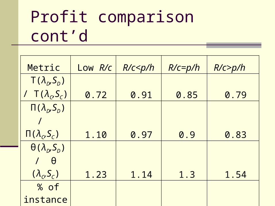
Profit comparison cont’d

Metric Low R/c R/c<p/h R/c=p/h R/c>p/hT(λD,SD)/ T(λC,SC) 0.72 0.91 0.85 0.79Π(λD,SD)

/ Π(λC,SC) 1.10 0.97 0.9 0.83θ(λD,SD)/ θ (λC,SC) 1.23 1.14 1.3 1.54

% of instances customer

loss 39 12 5 3

Conclusion

Developed a make-to-stock production system with strategic customers

Characterized customers’ equilibrium joining probability and producer’s optimal decision

Identified cases where centralization is profitable

Future Research

Fully observable system Finished the analysis of centralized and

decentralized problems Showed the concavity of producer’s profit

function Showed the optimality of base stock policy

and Partially observable system Comparison with pure queueing system

on a production/inventory system with strategic customers and unobservable inventory levels can oz...

Documents